Targeted vaccination strategies for an infinite-dimensional SIS model

Abstract.

We formalize and study the problem of optimal allocation strategies for a (perfect) vaccine in the infinite-dimensional SIS model. The question may be viewed as a bi-objective minimization problem, where one tries to minimize simultaneously the cost of the vaccination, and a loss that may be either the effective reproduction number, or the overall proportion of infected individuals in the endemic state. We prove the existence of Pareto optimal strategies for both loss functions.

We also show that vaccinating according to the profile of the endemic state is a critical allocation, in the sense that, if the initial reproduction number is larger than 1, then this vaccination strategy yields an effective reproduction number equal to $1$.

1. Introduction

1.1. Motivation

Increasing the prevalence of immunity from contagious disease in a population limits the circulation of the infection among the individuals who lack immunity. This so-called “herd effect” plays a fundamental role in epidemiology as it has had a major impact in the eradication of smallpox and rinderpest or the near eradication of poliomyelitis; see [19]. Targeted vaccination strategies, based on the heterogeneity of the infection spreading in the population, are designed to increase the level of immunity of the population with a limited quantity of vaccine. These strategies rely on identifying groups of individuals that should be vaccinated in priority in order to slow down or eradicate the disease.

In this article, we establish a theoretical framework to study targeted vaccination strategies for the deterministic infinite-dimensional SIS model introduced in [7], that encompasses as particular cases the SIS model on graphs or on stochastic block models. In companion papers, we provide a series of general and specific examples that complete and illustrate the present work: see Section 1.5 for more detail.

1.2. Herd immunity and targeted vaccination strategies

Let us start by recalling a few classical results in mathematical epidemiology; we refer to Keeling and Rohani’s monograph [30] for an extensive introduction to this field, including details on the various classical models (SIS, SIR, etc.)

In an homogeneous population, the basic reproduction number of an infection, denoted by $R_{0}$, is defined as the number of secondary cases one individual generates on average over the course of its infectious period, in an otherwise uninfected (susceptible) population. This number plays a fundamental role in epidemiology as it provides a scale to measure how difficult an infectious disease is to control. Intuitively, the disease should die out if $R_{0}<1$ and invade the population if $R_{0}>1$. For many classical mathematical models of epidemiology, such as SIS or S(E)IR, this intuition can be made rigorous: the quantity $R_{0}$ may be computed from the parameters of the model, and the threshold phenomenon occurs.

Assuming $R_{0}>1$ in an homogeneous population, suppose now that only a proportion $\eta^{\mathrm{uni}}$ of the population can catch the disease, the rest being immunized. An infected individual will now only generate $\eta^{\mathrm{uni}}R_{0}$ new cases, since a proportion $(1-\eta^{\mathrm{uni}})$ of previously successful infections will be prevented. Therefore, the new effective reproduction number is equal to $R_{e}(\eta^{\mathrm{uni}})=\eta^{\mathrm{uni}}R_{0}$. This fact led to the recognition by Smith in 1970 [42] and Dietz in 1975 [13] of a simple threshold theorem: the incidence of an infection declines if the proportion of non-immune individuals is reduced below $\eta^{\mathrm{uni}}_{\mathrm{crit}}=1/R_{0}$. This effect is called herd immunity, and the corresponding percentage $1-\eta^{\mathrm{uni}}_{\mathrm{crit}}$ of people that have to be vaccinated is called herd immunity threshold; see for instance [43, 44].

It is of course unrealistic to depict human populations as homogeneous, and many generalizations of the homogeneous model have been studied; see [30, Chapter 3] for examples and further references. For most of these generalizations, it is still possible to define a meaningful reproduction number $R_{0}$, as the number of secondary cases generated by a typical infectious individual when all other individuals are uninfected; see [12]. After a vaccination campaign, let the vaccination strategy $\eta$ denote the (non necessarily homogeneous) proportion of the non-vaccinated population, and let the effective reproduction number $R_{e}(\eta)$ denote the corresponding reproduction number of the non-vaccinated population. The vaccination strategy $\eta$ is critical if $R_{e}(\eta)=1$. The possible choices of $\eta$ naturally raises a question that may be expressed as the following informal optimization problem:

(1) $$\begin{cases}\textbf{Minimize: }&\text{the quantity of vaccine to administrate}\\ \textbf{subject to: }&\text{herd immunity is reached, that is,~{}$R_{e}\leq 1$.}\end{cases}$$

If the quantity of available vaccine is limited, then one is also interested in:

(2) $$\begin{cases}\textbf{Minimize: }&\text{the effective reproduction number~{}$R_{e}$}\\ \textbf{subject to: }&\text{a given quantity of available vaccine.}\end{cases}$$

Interestingly enough, the strategy $\eta^{\mathrm{uni}}_{\mathrm{crit}}$, which consists in delivering the vaccine uniformly to the population, without taking inhomogeneity into account, leaves a proportion $\eta^{\mathrm{uni}}_{\mathrm{crit}}=1/R_{0}$ of the population unprotected, and is therefore critical since $R_{e}(\eta^{\mathrm{uni}}_{\mathrm{crit}})=1$. In particular it is admissible for the optimization problem (1).

However, herd immunity may be achieved even if the proportion of unprotected people is greater than $1/R_{0}$, by targeting certain group(s) within the population; see Figure 3.3 in [30]. For example, the discussion of vaccination control of gonorrhea in [24, Section 4.5] suggests that it may be better to prioritize the vaccination of people that have already caught the disease: this lead us to consider a vaccination strategy guided by the equilibrium state. This strategy denoted by $\eta^{\mathrm{equi}}$ will be defined formally below. Let us mention here an observation in the same vein made by Britton, Ball and Trapman in [4]. Recall that in the S(E)IR model, immunity can be obtained through infection. Using parameters from real-world data, these authors noticed that the disease-induced herd immunity level can, for some models, be substantially lower than the classical herd immunity threshold $1-1/R_{0}$. This can be reformulated in term of targeted vaccination strategies: prioritizing the individuals that are more likely to get infected in a S(E)IR epidemic may be more efficient than distributing uniformly the vaccine in the population.

The main goal of this paper is two-fold: formalize the optimization problems (1) and (2) for a particular infinite dimensional SIS model, recasting them more generally as a bi-objective optimization problem; and give existence and properties of solutions to this bi-objective problem. We will also consider a closely related problem, where one wishes to minimize the size of the epidemic rather than the reproduction number. We will in passing provide insight on the efficiency of classical vaccination strategies such as $\eta^{\mathrm{uni}}_{\mathrm{crit}}$ or $\eta^{\mathrm{equi}}$.

1.3. Literature on targeted vaccination strategies

Targeted vaccination problems have mainly been studied using two different mathematical frameworks.

1.3.1. On meta-populations models

Problems (1) and (2) have been examined in depth for deterministic meta-population models, that is, models in which an heterogeneous population is stratified into a finite number of homogeneous sub-populations (by age group, gender, …). Such models are specified by choosing the sizes of the subpopulations and quantifying the degree of interactions between them, in terms of various mixing parameters. In this setting, $R_{0}$ can often be identified as the spectral radius of a next-generation matrix whose coefficients depend on the subpopulation sizes, and the mixing parameters. It turns out that the next generation matrices take similar forms for many dynamics (SIS, SIR, SEIR,…); see the discussion in [25, Section 10]. Vaccination strategies are defined as the levels at which each sub-population is immunized. After vaccination, the next-generation matrix is changed and its new spectral radius corresponds to the effective reproduction number $R_{e}$.

Problem (1) has been studied in this setting by Hill and Longini [25]. These authors study the geometric properties of the so-called threshold hypersurface, that is the vaccination allocations for which $R_{e}=1$. They also compute the vaccination belonging to this surface with minimal cost for an Influenza A model. Making structural assumptions on the mixing parameters, Poghotayan, Feng, Glasser and Hill derive in [38] an analytical formula for the solutions of Problem (2), for populations divided in two groups. Many papers also contain numerical studies of the optimization problems (1) and (2) on real-world data using gradient techniques or similar methods; see for example [21, 18, 14, 17, 47].

Finally, the effective reproduction number is not the only reasonable way of quantifying a population’s vulnerability to an infection. For an SIR infection for example, the proportion of individuals that eventually catch (and recover from) the disease, often referred to as the attack rate, is broadly used. We refer to [14, 15] for further discussion on this topic.

1.3.2. On networks

Whereas the previously cited works typically consider a small number of subpopulations, often with a “dense” structure of interaction (every subpopulation may directly infect all the others), other research communities have looked into a similar problem for graphs. Indeed, given a (large), possibly random graph, with epidemic dynamics on it, and supposing that we are able to suppress vertices by vaccinating, one may ask for the best way to choose the vertices to remove.

The importance of the spectral radius of the network has been rapidly identified as its value determines if the epidemic dies out quickly or survives for a long time [20, 39]. Since Van Mieghem et al. proved in [46] that the problem of minimizing spectral radius of a graph by removing a given number of vertices is NP-complete (and therefore unfeasible in practice), many computational heuristics have been put forward to give approximate solutions; see for example [40] and references therein.

1.4. Main results

The differential equations governing the epidemic dynamics in meta-population SIS models were developed by Lajmanovich and Yorke in their pioneer paper [33]. In [7], we introduced a natural generalization of their equation, which can also be viewed as the limit equation of the stochastic SIS dynamic on network, in an infinite-dimensional space $\Omega$, where $x\in\Omega$ represents a feature and the probability measure $\mu(\mathrm{d}x)$ represents the fraction of the population with feature $x$.

1.4.1. Regularity of the effective reproduction function $R_{e}$

We consider the effective reproduction function in a general operator framework which we call the kernel model. This model is characterized by a probability space $(\Omega,\mathscr{F},\mu)$ and a measurable non-negative kernel $\mathrm{k}:\Omega\times\Omega\rightarrow\mathbb{R}_{+}$. Let $T_{\mathrm{k}}$ be the corresponding integral operator defined by:

$$T_{\mathrm{k}}(h)(x)=\int_{\Omega}\mathrm{k}(x,y)h(y)\,\mu(\mathrm{d}y).$$

In the setting of [7] (see in particular Equation (11) therein), $T_{\mathrm{k}}$ is the so-called next generation operator, where the kernel $\mathrm{k}$ is defined in terms of a transmission rate kernel $k(x,y)$ and a recovery rate function $\gamma$ by the product $\mathrm{k}(x,y)=k(x,y)/\gamma(y)$; and the reproduction number $R_{0}$ is then the spectral radius $\rho(T_{\mathrm{k}})$ of $T_{\mathrm{k}}$.

Following [7, Section 5], we represent a vaccination strategy by a function $\eta:\Omega\rightarrow[0,1]$, where $\eta(x)$ represents the fraction of non-vaccinated individuals with feature $x$; the effective reproduction number associated to $\eta$ is then given by

(3) $$R_{e}(\eta)=\rho(T_{\mathrm{k}\eta}),$$

where $\rho$ stands for the spectral radius and $\mathrm{k}\eta$ stands for the kernel $(\mathrm{k}\eta)(x,y)=\mathrm{k}(x,y)\eta(y)$. If $R_{0}\geq 1$, then a vaccination strategy $\eta$ is called critical if it achieves precisely the herd immunity threshold, that is $R_{e}(\eta)=1$.

In particular, the “strategy” that consists in vaccinating no one corresponds to $\eta\equiv\mathds{1}$, and of course $R_{e}(\mathds{1})=R_{0}$. As the spectral radius is positively homogeneous, we also get, when $R_{0}\geq 1$, that the uniform strategy that corresponds to the constant function:

$$\eta^{\mathrm{uni}}_{\mathrm{crit}}\equiv\frac{1}{R_{0}}$$

is critical, as $R_{e}(\eta^{\mathrm{uni}}_{\mathrm{crit}})=1$. This is consistent with results obtained in the homogeneous model given in Section 1.2.

Let $\Delta$ be the set of strategies, that is the set of $[0,1]$-valued functions defined on $\Omega$. The usual technique to obtain the existence of solutions to optimization problems like (1) or (2) is to prove that the function $R_{e}$ is continuous with respect to a topology for which the set of strategies $\Delta$ is compact. It is natural to try and prove this continuity by writing $R_{e}$ as the composition of the spectral radius $\rho$ and the map $\eta\mapsto T_{\mathrm{k}\eta}$. The spectral radius is indeed continuous at compact operators (and $T_{\mathrm{k}\eta}$ is in fact compact under a technical integrability assumption on the kernel $\mathrm{k}$ formalized on page 1 as Assumption 1), if we endow the set of bounded operators with the operator norm topology; see [37, 5]. However, this would require choosing the uniform topology on $\Delta$, which then is not compact.

We instead endow $\Delta$ with the weak topology, see Section 3.1, for which compactness holds; see Lemma 3.1. This forces us to equip the space of bounded operators with the strong topology, for which the spectral radius is in general not continuous; see [29, p. 431]. However, the family of operators $(T_{\mathrm{k}\eta},\,\eta\in\Delta)$ is collectively compact which enables us to recover continuity, using a serie of results obtained by Anselone [1]. This leads to the following result, proved in Theorem 4.2 below. We recall that Assumption 1, formulated on page 1, provides an integrability condition on the kernel $\mathrm{k}$.

Theorem 1.1 (Continuity of the spectral radius).

Under Assumption 1 on the kernel $\mathrm{k}$, the function $R_{e}\,\colon\,\Delta\to\mathbb{R}_{+}$ is continuous with respect to the weak topology on $\Delta$.

In fact, we also prove the continuity of the spectrum with respect to the Hausdorff distance on the set of compact subsets of $\mathbb{C}$. We shall write $R_{e}[\mathrm{k}]$ to stress the dependence of the function $R_{e}$ in the kernel $\mathrm{k}$. In Proposition 4.3, we prove the stability of $R_{e}$, by giving natural sufficient conditions on a sequence of kernels $(\mathrm{k}_{n},n\in\mathbb{N})$ converging to $\mathrm{k}$ which imply that $R_{e}[\mathrm{k}_{n}]$ converges uniformly towards $R_{e}[\mathrm{k}]$. This result has both theoretical and practical interest: the next-generation operator is unknown in practice, and has to be estimated from data. Thanks to this result, the value of $R_{e}$ computed from the estimated operator should converge to the true value.

1.4.2. On the maximal endemic equilibrium in the SIS model

We consider the SIS model from [7]. This model is characterized by a probability space $(\Omega,\mathscr{F},\mu)$, the transmission kernel $k\,\colon\,\Omega\times\Omega\to\mathbb{R}_{+}$ and the recovery rate $\gamma\,\colon\,\Omega\to\mathbb{R}_{+}^{*}$. We suppose in the following that the technical Assumption 2, formulated on page 2, holds, so that the SIS dynamical evolution is well defined.

This evolution is encoded as $u=(u_{t},t\in\mathbb{R}_{+})$, where $u_{t}\in\Delta$ for all $t$ and $u_{t}(x)$ represents the probability of an individual with feature $x\in\Omega$ to be infected at time $t\geq 0$, and follows the equation:

(4) $$\partial_{t}u_{t}=F(u_{t})\quad\text{for }t\in\mathbb{R}_{+},\quad\text{where}\quad F(g)=(1-g)\mathcal{T}_{k}(g)-\gamma g\quad\text{for }g\in\Delta,$$

with an initial condition $u_{0}\in\Delta$ and with $\mathcal{T}_{k}$ the integral operator corresponding to the kernel $k$ acting on the set of bounded measurable functions, see (16). It is proved in [7] that such a solution $u$ exists and is unique under Assumption 2. An equilibrium of (4) is a function $g\in\Delta$ such that $F(g)=0$. According to [7], there exists a maximal equilibrium $\mathfrak{g}$, i.e., an equilibrium such that all other equilibria $h\in\Delta$ are dominated by $\mathfrak{g}$: $h\leq\mathfrak{g}$. Furthermore, we have $R_{0}\leq 1$ if and only if $\mathfrak{g}=0$. In the connected case (for example if $k>0$), then $0$ and $\mathfrak{g}$ are the only equilibria; besides $\mathfrak{g}$ is the long-time distribution of infected individuals in the population: $\lim_{t\rightarrow+\infty}u_{t}=\mathfrak{g}$ as soon as the initial condition is non-zero; see [7, Theorem 4.14].

As hinted in [24, Section 4.5] for vaccination control of gonorrhea, it is interesting to consider vaccinating people with feature $x$ with probability $\mathfrak{g}(x)$; this corresponds to the strategy based on the maximal equilibrium:

$$\eta^{\mathrm{equi}}=1-\mathfrak{g}.$$

The following result entails that this strategy is critical and thus achieves the herd immunity threshold. Recall that Assumption 2, formulated page 2, provides technical conditions on the parameters $k$ and $\gamma$ of the SIS model. The effective reproduction number of the SIS model is the function $R_{e}$ defined in (3) with the kernel $\mathrm{k}=k/\gamma$.

Theorem 1.2 (The maximal equilibrium yields a critical vaccination).

Suppose Assumption 2 holds. If $R_{0}\geq 1$, then the vaccination strategy $\eta^{\mathrm{equi}}$ is critical, that is, $R_{e}(\eta^{\mathrm{equi}})=1$.

This result will be proved below as a part of Proposition 8.2. Let us finally describe informally another consequence of this Proposition. We were able to prove in [7, Theorem 4.14] that, in the connected case, if $R_{0}>1$, the disease-free equilibrium $u=0$ is unstable. Proposition 8.2 gives spectral information on the formal linearization of the dynamics (4) near any equilibrium $h$; in particular if $h\neq\mathfrak{g}$ then $h$ is linearly unstable.

1.4.3. Regularity of the total proportion of infected population function $\mathfrak{I}$

According to [7, Section 5.3.], the SIS equation with vaccination strategy $\eta$ is given by (4), where $F$ is replaced by $F_{\eta}$ defined by:

$$F_{\eta}(g)=(1-g)T_{k\eta}(g)-\gamma g.$$

and $u_{t}$ now describes the proportion of infected among the non-vaccinated population. We denote by $\mathfrak{g}_{\eta}$ the corresponding maximal equilibrium (thus considering $\eta\equiv 1$ gives $\mathfrak{g}=\mathfrak{g}_{1}$), so that $F_{\eta}(\mathfrak{g}_{\eta})=0$. Since the probability for an individual $x$ to be infected in the stationary regime is $\mathfrak{g}_{\eta}(x)\,\eta(x)$, the fraction of infected individuals at equilibrium, $\mathfrak{I}(\eta)$, is thus given by:

(5) $$\mathfrak{I}(\eta)=\int_{\Omega}\mathfrak{g}_{\eta}\,\eta\,\mathrm{d}\mu=\int_{\Omega}\mathfrak{g}_{\eta}(x)\,\eta(x)\,\mu(\mathrm{d}x).$$

As mentioned above, for a SIR model, distributing vaccine so as to minimize the attack rate is at least as natural as trying to minimize the reproduction number, and this problem has been studied for example in [14, 15]. In the SIS model the quantity $\mathfrak{I}$ appears as a natural analogue of the attack rate, and is therefore a natural optimization objective.

We obtain results on $\mathfrak{I}$ that are very similar to the ones on $R_{e}$. Recall that Assumption 2 on page 2 ensures that the infinite-dimensional SIS model, given by equation (4), is well defined. The next theorem corresponds to Theorem 4.6.

Theorem 1.3 (Continuity of the equilibrium infection size).

Under Assumption 2, the function $\mathfrak{I}\,\colon\,\Delta\to\mathbb{R}_{+}$ is continuous with respect to the weak topology on $\Delta$.

In Proposition 4.7, we prove the stability of $\mathfrak{I}$, by giving natural sufficient condition on a sequence of kernels and functions $((k_{n},\gamma_{n}),n\in\mathbb{N})$ converging to $(k,\gamma)$ which imply that $\mathfrak{I}[k_{n},\gamma_{n}]$ converges uniformly towards $\mathfrak{I}[k,\gamma]$. We also prove that the loss functions $\mathrm{L}=R_{e}$ and $\mathrm{L}=\mathfrak{I}$ are both non-decreasing ($\eta\leq\eta^{\prime}$ implies $\mathrm{L}(\eta)\leq\mathrm{L}(\eta^{\prime})$), and sub-homogeneous ($\mathrm{L}(\lambda\eta)\leq\lambda\mathrm{L}(\eta)$ for all $\lambda\in[0,1]$); see Propositions 4.1 and 4.5.

1.4.4. Optimizing the protection of the population

Consider a cost function $C\,\colon\,\Delta\to[0,1]$ which measures the cost for the society of a vaccination strategy (production and diffusion). Since the vaccination strategy $\eta$ represents the non-vaccinated population, the cost function $C$ should be decreasing (roughly speaking $\eta<\eta^{\prime}$ implies $C(\eta)>C(\eta^{\prime})$; see Definition 5.1). We shall also assume that $C$ is continuous with respect to the weak topology on $\Delta$, and that doing nothing costs nothing, that is, $C(\mathds{1})=0$. A simple and natural choice is the uniform cost $C_{\mathrm{uni}}$ given by the overall proportion of vaccinated individuals:

$$C_{\mathrm{uni}}(\eta)=\int_{\Omega}(1-\eta)\,\mathrm{d}\mu=1-\int_{\Omega}\eta\,\mathrm{d}\mu.$$

See Remark 5.2 for comments on other examples of cost functions.

Our problem may now be seen as a bi-objective minimization problem: we wish to minimize both the loss $\mathrm{L}(\eta)$ and the cost $C(\eta)$, subject to $\eta\in\Delta$, with the loss function $\mathrm{L}$ being either $R_{e}$ or $\mathfrak{I}$. Following classical terminology for multi-objective optimisation problems [36], we call a strategy $\eta_{\star}$ Pareto optimal if no other strategy is strictly better:

$$C(\eta)<C(\eta_{\star})\implies\mathrm{L}(\eta)>\mathrm{L}(\eta_{\star})\quad\text{and}\quad\mathrm{L}(\eta)<\mathrm{L}(\eta_{\star})\implies C(\eta)>C(\eta_{\star}).$$

The set of Pareto optimal strategies will be denoted by $\mathcal{P}_{\mathrm{L}}$, and we define the Pareto frontier as the set of Pareto optimal outcomes:

$$\mathcal{F}_{\mathrm{L}}=\{(C(\eta_{\star}),\mathrm{L}(\eta_{\star}))\,\colon\,\eta_{\star}\in\mathcal{P}_{\mathrm{L}}\}.$$

Notice that, with this definition, the Pareto frontier is empty when there is no Pareto optimal strategy.

For any strategy $\eta$, the cost and loss of $\eta$ vary between the following bounds:

$$0=C(\mathds{1})\leq C(\eta)\leq C(0)=c_{\max}=\text{cost of vaccinating the whole population},$$

$$0=\mathrm{L}(0)\leq\mathrm{L}(\eta)\leq\mathrm{L}(\mathds{1})=\ell_{\max}=\text{loss incurred in the absence of vaccination}.$$

Let $\mathrm{L}_{\star}$ be the optimal loss function and $C_{\star,\mathrm{L}}$ the optimal cost function defined by:

$$\mathrm{L}_{\star}(c) =\inf\,\set{\mathrm{L}(\eta)\,\colon\,\eta\in\Delta,\,C(\eta)\leq c}\quad\text{for $c\in[0,c_{\max}]$},$$

$$C_{\star,\mathrm{L}}(\ell) =\inf\,\set{C(\eta)\,\colon\,\eta\in\Delta,\,\mathrm{L}(\eta)\leq\ell}\quad\text{for $\ell\in[0,\ell_{\max}]$}.$$

We simply write $C_{\star}$ for $C_{\star,\mathrm{L}}$ when no confusion on the loss function can arise. Proposition 5.5 (in a more general framework in particular for the cost function) and Lemma 5.6 states that the Pareto frontier is non empty and has a continuous parametrization for the cost $C=C_{\mathrm{uni}}$ and the loss $\mathrm{L}=R_{e}$ or $\mathrm{L}=\mathfrak{I}$; see Figure 1(b) below for a visualization of the Pareto frontier.

Theorem 1.4 (Properties of the Pareto frontier).

For the kernel model with loss function $\mathrm{L}=R_{e}$ or the SIS model with $\mathrm{L}\in\{R_{e},\mathfrak{I}\}$, and the uniform cost function $C=C_{\mathrm{uni}}$, the function $C_{\star,\mathrm{L}}$ is continuous and decreasing on $[0,\ell_{\max}]$, the function $\mathrm{L}_{\star}$ is continuous on $[0,c_{\max}]$ decreasing on $[0,C_{\star,\mathrm{L}}(0)]$ and zero on $[C_{\star,\mathrm{L}}(0),c_{\max}]$; furthermore the Pareto frontier is connected and:

$$\mathcal{F}_{\mathrm{L}}=\{(c,\mathrm{L}_{\star}(c))\,\colon\,c\in[0,C_{\star,\mathrm{L}}(0)]\}=\{(C_{\star,\mathrm{L}}(\ell),\ell)\,\colon\,\ell\in[0,\ell_{\max}]\}.$$

We also establish that $\mathcal{P}_{\mathrm{L}}$ is compact in $\Delta$ for the weak topology in Corollary 5.7; that the set of outcomes or feasible region $\mathbf{F}=\{(C(\eta),\mathrm{L}(\eta)),\,\eta\in\Delta\}$ has no holes in Proposition 6.1; and that the Pareto frontier is convex if $C$ and $\mathrm{L}$ are convex in Proposition 6.6. We study in Proposition 6.2 the stability of the Pareto frontier and the set of Pareto optima when the parameters vary.

In a sense the Pareto optimal strategies are intuitively the “best” strategies. Similarly, we also study the “worst” strategies, which we call anti-Pareto optimal strategies, and describe the corresponding anti-Pareto frontier. Understanding the “worst strategies” also helps to avoid pitfalls when one has to consider sub-optimal strategies: for example, we prove in [8] that disconnecting strategies are not the “worst” strategies, and we provide in [10, Section 4] an elementary example where the same strategies can be “best” or “worst” according to model parameters values. Surprisingly, proving properties of the anti-Pareto frontier sometimes necessitates stronger assumptions than in the Pareto case: for example, the connectedness of the anti-Pareto frontier is only proved under a quasi-irreducibility assumption on the kernel, see Lemmas 5.11 and 5.12.

Remark 1.5 (Eradication strategies do not depend on the loss).

In [7], we proved that, for all $\eta\in\Delta$, the equilibrium infection size $\mathfrak{I}(\eta)$ is non zero if and only if $R_{e}(\eta)>1$. Consider the uniform cost $C=C_{\mathrm{uni}}$. First, this implies that $\mathcal{P}_{\mathfrak{I}}$ is a subset of $\{\eta\in\Delta\,\colon\,R_{e}(\eta)\geq 1\}$. Secondly, a vaccination strategy $\eta\in\Delta$ is Pareto optimal for the objectives $(R_{e},C)$ and satisfies $R_{e}(\eta)=1$ if and only if $\eta$ is Pareto optimal for the objectives $(\mathfrak{I},C)$ and satisfies $\mathfrak{I}(\eta)=0$:

(6) $$\eta\in\mathcal{P}_{R_{e}}\text{ and }R_{e}(\eta)=1\quad\Longleftrightarrow\quad\eta\in\mathcal{P}_{\mathfrak{I}}\text{ and }\mathfrak{I}(\eta)=0.$$

Remark 1.6 (Minimal cost of eradication).

Assume $R_{0}>1$ and the uniform cost $C=C_{\mathrm{uni}}$. The equivalence (6) implies directly that:

$$C_{\star,R_{e}}(\mathds{1})=C_{\star,\mathfrak{I}}(0).$$

Thus, this latter quantity can be seen as the minimal cost (or minimum percentage of people that have to be vaccinated) required to eradicate the infection. Recall the critical vaccination strategies $\eta^{\mathrm{uni}}_{\mathrm{crit}}\equiv 1/R_{0}$ and $\eta^{\mathrm{equi}}=1-\mathfrak{g}$ (as $R_{e}(\eta^{\mathrm{uni}}_{\mathrm{crit}})=R_{e}(\eta^{\mathrm{equi}})=1$). Since $C(\eta^{\mathrm{uni}}_{\mathrm{crit}})=1-1/R_{0}$ and  $C(\eta^{\mathrm{equi}})=\int_{\Omega}\mathfrak{g}\,\mathrm{d}\mu=\mathfrak{I}(\mathds{1})$, we obtain the following upper bounds of the minimal cost required to eradicate the infection:

$$C_{\star,R_{e}}(\mathds{1})=C_{\star,\mathfrak{I}}(0)\leq\min\left(1-\frac{1}{R_{0}}\,,\,\int_{\Omega}\mathfrak{g}\,\mathrm{d}\mu\right).$$

1.4.5. Equivalence of models

Our last results address a natural question stemming from our choice of a very general framework to modelize the infection. Since our models are infinite dimensional and depend on the choices of the probability space $(\Omega,\mathscr{F},\mu)$, the kernel $\mathrm{k}$ (for the kernel model) and the kernel $k$ and recovery rate $\gamma$ (for the SIS model), the are different equivalent ways to model the same situation. We study in Section 7 a way to ensure that, even if the parameters are different, we end up with the same Pareto frontiers. This situation is similar to random variables having the same law in probability theory, or to equivalent graphons in graphon theory. In particular it allows us to treat the same meta-population model in either a discrete or a continuous setting, see Figure 4 for an illustration and Example 1.7.

1.4.6. An illustrative example: the multipartite graphon

Let us illustrate some of our results on an example, which will be discussed in details in a forthcoming companion paper [10].

Example 1.7 (Multipartite graphon).

Graphs that can be colored with $\ell$ colors, so that no two endpoints of an edge have the same color are known as $\ell$-partite graphs. In a biological setting, this corresponds to a population of $\ell$ groups, such that individuals in a group can not contaminate individuals of the same group. Let us generalize and assume there is an infinity of groups, $\ell=\infty$ of respective size $(2^{-n},\,n\in\mathbb{N}^{*})$ and that the next generation kernel $\mathrm{k}$ is equal to the constant $\kappa>0$ between individuals of different groups and equal to $0$ between individuals of the same group (so there is no intra-group contamination). Using the equivalence of models from Section 7, we can represent this model by using a continuous state space $\Omega=[0,1]$, endowed with $\mu$ the Lebesgue measure on $\Omega$, the group $n$ being represented by the interval $I_{n}=[1-2^{-n+1},1-2^{-n})$ for $n\in\mathbb{N}^{*}$. The kernel $\mathrm{k}$ is then given by $\mathrm{k}=\kappa(1-\sum_{n\in\mathbb{N}^{*}}\mathds{1}_{I_{n}\times I_{n}})$; it is represented in Figure 1(a).

Consider the loss $\mathrm{L}=R_{e}$ and the cost $C=C_{\mathrm{uni}}$ giving the overall proportion of vaccinated individuals. Based on the results of [16, 45], we prove in [10] that the vaccination strategies $\mathds{1}_{[0,1-c]}$, with cost $C(\mathds{1}_{[0,1-c]})=c\in[0,1/2]$, are Pareto optimal. Remembering that the natural definition of the degree in a continuous graph is given by $\mathrm{deg}(x)=\int_{\Omega}\mathrm{k}(x,y)\,\mu(\mathrm{d}y)$, we note that the vaccination strategy $\mathds{1}_{[0,1-c]}$ corresponds to vaccinating individuals with feature $x\in(1-c,1]$, that is, the individuals with the highest degree. In Figure 1(b), the corresponding Pareto frontier (i.e., the outcome of the “best” vaccination strategies) is drawn as the solid red line; the blue-colored zone corresponds to the feasible region that is, all the possible values of $(C(\eta),R_{e}(\eta))$, where $\eta$ ranges over $\Delta$; the dotted line corresponds to the outcome of the uniform vaccination strategy $\eta\equiv c$, that is $(C(\eta),R_{e}(\eta))=(c,(1-c)R_{0})$ where $c$ ranges over $[0,1]$; and the red dashed curve corresponds to the anti-Pareto frontier (i.e., the outcome of the “worst” vaccination strategies), which for this model correspond to the uniform vaccination of the nodes with the updated lower degree; see [10]. Notice that the path $(\mathds{1}_{[0,1-c]},\,c\in[0,1/2])$ is an increasing continuous (for the topology of the simple convergence and thus the $L^{1}(\mu)$ topology) path of Pareto optima which gives a complete parametrization of the Pareto frontier. The latter has been computed numerically using the power iteration method. In particular, we obtained the following value: $R_{0}\simeq 0.697\kappa$.

(a) Grayplot of the kernel $\mathrm{k}$, with $\Omega=[0,1]$ and $\mu$ the Lebesgue measure ($\mathrm{k}$ is equal to the constant $\kappa>0$ on the black zone and to $0$ on the white zone).

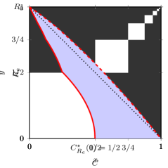
(b) The Pareto frontier in solid red line compared to the cost and loss of the uniform vaccinations in dotted line and the worst vaccination strategy in red dashed line.

Figure 1. Example of optimization with $\mathrm{L}=R_{e}$.

1.5. On the companion papers

We detail some developments in forthcoming papers where only the uniform cost $C=C_{\mathrm{uni}}$ is considered. In [8], motivated by the conjecture formulated by Hill and Longini in finite dimension [25, Conjecture 8.1], we investigate the convexity and concavity of the effective reproduction function $R_{e}$. We also prove that a disconnecting strategy is better than the worst, i.e., is not anti-Pareto optimal.

In [11], under monotonicity properties of the kernel, satisfied for example by the configuration model, it is proven that vaccinating the individuals with the highest (resp. lowest) number of contacts is Pareto (resp. anti-Pareto) optimal. In this case the greedy algorithm, which performs infinitesimal locally optimal steps, is optimal as it browses continuously the set of Pareto (resp. anti-Pareto) optimal strategies, providing an increasing parametrization of the Pareto (resp. anti-Pareto) frontier. In this setting, we provide some examples of SIS models where the set of Pareto optimal strategies coincide for the losses $R_{e}$ and $\mathfrak{I}$:

(7) $$\mathcal{P}_{\mathfrak{I}}=\mathcal{P}_{R_{e}}\cap\{\eta\in\Delta\,\colon\,R_{e}(\eta)\geq 1\}.$$

In [10], which includes a detailed study of the multipartite kernel of Example 1.7, we study the optimal vaccination when the individuals have the same number of contacts. This provides examples where the uniform vaccination is Pareto optimal, or anti-Pareto optimal, or not optimal for either problem. We also provide an example where the set $\mathcal{P}_{R_{e}}$ has a countable number of connected components (and is thus not connected). This implies in particular that the greedy algorithm is not optimal in this case.

In [9], we give a comprehensive treatment of the two groups model, $\Omega=\{1,2\}$, for $\mathrm{L}=R_{e}$, and some partial results for $\mathrm{L}=\mathfrak{I}$. Despite its apparent simplicity, the derivation of formulae for the Pareto optimal strategies is non trivial, see also [38]. In addition, this model is rich enough to give examples of various interesting behaviours:

• On the critical strategies $\eta^{\mathrm{uni}}_{\mathrm{crit}}$ and $\eta^{\mathrm{equi}}$. Depending on the parameters, the strategies $\eta^{\mathrm{uni}}_{\mathrm{crit}}$ and/or $\eta^{\mathrm{equi}}$ may or may not be Pareto optimal, and the cost $C(\eta^{\mathrm{uni}}_{\mathrm{crit}})$ may be larger than, smaller than or equal to $C(\eta^{\mathrm{equi}})$.

• Vaccinating people with highest contacts. The intuitive idea of vaccinating the individuals with the highest number of contacts may or may not provide the optimal strategies, depending on the parameters.

• Dependence on the choice of the loss function. For examples where $R_{0}>1$, the optimal strategies for the losses $\mathfrak{I}$ and $R_{e}$ may coincide, so that (7) holds, or not at all, so that $\mathcal{P}_{\mathfrak{I}}\cap\mathcal{P}_{R_{e}}\cap\{\eta\in\Delta\,\colon\,1<R_{e}(\eta)<R_{0}\}=\emptyset$, depending on the parameters.

1.6. Structure of the paper

Section 2 is dedicated to the presentation of the vaccination model and the various assumptions on the parameters. We also define properly the so-called loss functions $R_{e}$ and $\mathfrak{I}$. After recalling a few topological facts in Section 3, we study the regularity properties of $R_{e}$ and $\mathfrak{I}$ in Section 4. We present the multi-objective optimization problem in Section 5 under general condition on the loss function $\mathrm{L}$ and cost function $C$ and prove the results on the Pareto frontier. This is completed in Section 6 with miscellaneous properties of the Pareto frontier. In Section 7, we discuss the equivalent representation of models with different parameters. Proofs of a few technical results are gathered in Section 8.

2. Setting and notation

2.1. Spaces, operators, spectra

All metric spaces $(S,d)$ are endowed with their Borel $\sigma$-field denoted by $\mathscr{B}(S)$. The set $\mathscr{K}$ of compact subsets of $\mathbb{C}$ endowed with the Hausdorff distance $d_{\mathrm{H}}$ is a metric space, and the function $\mathrm{rad}$ from $\mathscr{K}$ to $\mathbb{R}_{+}$ defined by $\mathrm{rad}(K)=\max\{|\lambda|\,,\,\lambda\in K\}$ is Lipschitz continuous from $(\mathscr{K},d_{\mathrm{H}})$ to $\mathbb{R}$ endowed with its usual Euclidean distance.

Let $(\Omega,\mathscr{F},\mu)$ be a probability space. We denote by $\mathscr{L}^{\infty}$, the Banach spaces of bounded real-valued measurable functions defined on $\Omega$ equipped with the $\sup$-norm, $\mathscr{L}^{\infty}_{+}$ the subset of $\mathscr{L}^{\infty}$ of non-negative function, and $\Delta=\{f\in\mathscr{L}^{\infty}\,\colon\,0\leq f\leq 1\}$ the subset of non-negative functions bounded by $1$. For $f$ and $g$ real-valued functions defined on $\Omega$, we may write $\langle f,g\rangle$ or $\int_{\Omega}fg\,\mathrm{d}\mu$ for $\int_{\Omega}f(x)g(x)\,\mu(\mathrm{d}x)$ whenever the latter is meaningful. For $p\in[1,+\infty]$, we denote by $L^{p}=L^{p}(\mu)=L^{p}(\Omega,\mu)$ the space of real-valued measurable functions $g$ defined $\Omega$ such that $\lVert g\rVert_{p}=\left(\int|g|^{p}\,\mathrm{d}\mu\right)^{1/p}$ (with the convention that $\lVert g\rVert_{\infty}$ is the $\mu$-essential supremum of $|g|$) is finite, where functions which agree $\mu$-almost surely are identified. We denote by $L^{p}_{+}$ the subset of $L^{p}$ of non-negative functions.

Let $(E,\lVert\cdot\rVert)$ be a Banach space. We denote by $\lVert\cdot\rVert_{E}$ the operator norm on $\mathcal{L}(E)$ the Banach algebra of bounded operators. The spectrum $\operatorname{Spec}(T)$ of $T\in\mathcal{L}(E)$ is the set of $\lambda\in\mathbb{C}$ such that $T-\lambda\mathrm{Id}$ does not have a bounded inverse operator, where $\mathrm{Id}$ is the identity operator on $E$. Recall that $\operatorname{Spec}(T)$ is a compact subset of $\mathbb{C}$, and that the spectral radius of $T$ is given by:

(8) $$\rho(T)=\mathrm{rad}(\operatorname{Spec}(T))=\lim_{n\rightarrow\infty}\lVert T^{n}\rVert_{E}^{1/n}.$$

The element $\lambda\in\operatorname{Spec}(T)$ is an eigenvalue if there exists $x\in E$ such that $Tx=\lambda x$ and $x\neq 0$.

If $E$ is also a functional space, for $g\in E$, we denote by $M_{g}$ the multiplication (possibly unbounded) operator defined by $M_{g}(h)=gh$ for all $h\in E$.

2.2. Kernel operators

We define a kernel (resp. signed kernel) on $\Omega$ as a $\mathbb{R}_{+}$-valued (resp. $\mathbb{R}$-valued) measurable function defined on $(\Omega^{2},\mathscr{F}^{\otimes 2})$. For $f,g$ two non-negative measurable functions defined on $\Omega$ and $\mathrm{k}$ a kernel on $\Omega$, we denote by $f\mathrm{k}g$ the kernel defined by:

(9) $$f\mathrm{k}g:(x,y)\mapsto f(x)\,\mathrm{k}(x,y)g(y).$$

When $\gamma$ is a positive measurable function defined on $\Omega$, we write $\mathrm{k}/\gamma$ for $\mathrm{k}\gamma^{-1}$, and remark that it may differ from $\gamma^{-1}\mathrm{k}$.

For $p\in(1,+\infty)$, we define the double norm of a signed kernel $\mathrm{k}$ by:

(10) $$\lVert\mathrm{k}\rVert_{p,q}=\left(\int_{\Omega}\left(\int_{\Omega}\lvert\mathrm{k}(x,y)\rvert^{q}\,\mu(\mathrm{d}y)\right)^{p/q}\mu(\mathrm{d}x)\right)^{1/p}\quad\text{with~{}$q$ given by}\quad\frac{1}{p}+\frac{1}{q}=1.$$

Assumption 1 (On the kernel model $[(\Omega,\mathscr{F},\mu),\mathrm{k}]$).

Let $(\Omega,\mathscr{F},\mu)$ be a probability space. The kernel $\mathrm{k}$ on $\Omega$ has a finite double-norm, that is, $\lVert\mathrm{k}\rVert_{p,q}<+\infty$ for some $p\in(1,+\infty)$.

To a kernel $k$ such that $\lVert\mathrm{k}\rVert_{p,q}<+\infty$, we associate the positive integral operator $T_{\mathrm{k}}$ on $L^{p}$ defined by:

(11) $$T_{\mathrm{k}}(g)(x)=\int_{\Omega}\mathrm{k}(x,y)g(y)\,\mu(\mathrm{d}y)\quad\text{for }g\in L^{p}\text{ and }x\in\Omega.$$

According to [22, p. 293], operator $T_{\mathrm{k}}$ is compact. It is well known and easy to check that:

(12) $$\lVert T_{\mathrm{k}}\rVert_{L^{p}}\leq\lVert\mathrm{k}\rVert_{p,q}.$$

For $\eta\in\Delta$, the kernel $\mathrm{k}\eta$ has also a finite double norm on $L^{p}$ and the operator $M_{\eta}$ is bounded, so that the operator $T_{\mathrm{k}\eta}=T_{\mathrm{k}}M_{\eta}$ is compact. We can define the effective spectrum function $\operatorname{Spec}[\mathrm{k}]$ from $\Delta$ to $\mathscr{K}$ by:

(13) $$\operatorname{Spec}[\mathrm{k}](\eta)=\operatorname{Spec}(T_{\mathrm{k}\eta}),$$

the effective reproduction number function $R_{e}[\mathrm{k}]=\mathrm{rad}\circ\operatorname{Spec}[\mathrm{k}]$ from $\Delta$ to $\mathbb{R}_{+}$ by:

(14) $$R_{e}[\mathrm{k}](\eta)=\mathrm{rad}(\operatorname{Spec}(T_{\mathrm{k}\eta}))=\rho(T_{\mathrm{k}\eta}),$$

and the corresponding reproduction number:

(15) $$R_{0}[\mathrm{k}]=R_{e}[\mathrm{k}](\mathds{1})=\rho(T_{\mathrm{k}}).$$

When there is no ambiguity, we simply write $R_{e}$ for $R_{e}[\mathrm{k}]$ and $R_{0}$ for $R_{0}[\mathrm{k}]$. We say a vaccination strategy $\eta\in\Delta$ is critical if $R_{e}(\eta)=1$.

Following the framework of [7], for $q\in(1,+\infty)$, we also consider the following norm for the kernel $\mathrm{k}$:

$$\lVert\mathrm{k}\rVert_{\infty,q}=\sup\limits_{x\in\Omega}\left(\int_{\Omega}\mathrm{k}(x,y)^{q}\,\mu(\mathrm{d}y)\right)^{1/q}.$$

Clearly, we have that $\lVert\mathrm{k}\rVert_{\infty,q}$ finite implies that $\lVert\mathrm{k}\rVert_{p,q}$ is also finite, with $p$ such that $1/p+1/q=1$. When $\lVert\mathrm{k}\rVert_{\infty,q}<+\infty$, the corresponding positive bounded linear integral operator $\mathcal{T}_{\mathrm{k}}$ on $\mathscr{L}^{\infty}$ is similarly defined by:

(16) $$\mathcal{T}_{\mathrm{k}}(g)(x)=\int_{\Omega}\mathrm{k}(x,y)g(y)\,\mu(\mathrm{d}y)\quad\text{for }g\in\mathscr{L}^{\infty}\text{ and }x\in\Omega.$$

Notice that the integral operators $\mathcal{T}_{\mathrm{k}}$ and $T_{\mathrm{k}}$ corresponds respectively to the operators $T_{\mathrm{k}}$ and $\hat{T}_{\mathrm{k}}$ in [7]. According to [7, Lemma 3.7], the operator $\mathcal{T}_{\mathrm{k}}^{2}$ on $\mathscr{L}^{\infty}$ is compact and $\mathcal{T}_{\mathrm{k}}$ has the same spectral radius as $T_{\mathrm{k}}$:

(17) $$\rho(\mathcal{T}_{\mathrm{k}})=\rho(T_{\mathrm{k}}).$$

2.3. Dynamics for the SIS model and equilibria

In accordance with [7], we consider the following assumption. Recall that $k/\gamma=k\gamma^{-1}$.

Assumption 2 (On the SIS model $[(\Omega,\mathscr{F},\mu),k,\gamma]$).

Let $(\Omega,\mathscr{F},\mu)$ be a probability space. The recovery rate function $\gamma$ is a function which belongs to $\mathscr{L}^{\infty}_{+}$ and the transmission rate kernel $k$ on $\Omega^{2}$ is such that $\lVert k/\gamma\rVert_{\infty,q}<+\infty$ for some $q\in(1,+\infty)$.

Assumption 2 implies Assumption 1 for the kernel $\mathrm{k}=k/\gamma$. Under Assumption 2, we also consider the bounded operators $\mathcal{T}_{k/\gamma}$ on $\mathscr{L}^{\infty}$, as well as $T_{k/\gamma}$ on $L^{p}$, which are the so called next-generation operator. The SIS dynamics considered in [7] (under Assumption 2) follows the vector field $F$ defined on $\mathscr{L}^{\infty}$ by:

(18) $$F(g)=(1-g)\mathcal{T}_{k}(g)-\gamma g.$$

More precisely, we consider $u=(u_{t},t\in\mathbb{R})$, where $u_{t}\in\Delta$ for all $t\in\mathbb{R}_{+}$ such that:

(19) $$\partial_{t}u_{t}=F(u_{t})\quad\text{for }t\in\mathbb{R}_{+},$$

with initial condition $u_{0}\in\Delta$. The value $u_{t}(x)$ models the probability that an individual of feature $x$ is infected at time $t$; it is proved in [7] that such a solution $u$ exists and is unique.

An equilibrium of (19) is a function $g\in\Delta$ such that $F(g)=0$. According to [7], there exists a maximal equilibrium $\mathfrak{g}$, i.e., an equilibrium such that all other equilibria $h\in\Delta$ are dominated by $\mathfrak{g}$: $h\leq\mathfrak{g}$. The reproduction number $R_{0}$ associated to the SIS model given by (19) is the spectral radius of the next-generation operator, so that using the definition of the effective reproduction number (14), (15) and (17), this amounts to:

(20) $$R_{0}=\rho(\mathcal{T}_{k/\gamma})=R_{0}[k/\gamma]=R_{e}[k/\gamma](\mathds{1}).$$

If $R_{0}\leq 1$ (sub-critical and critical case), then $u_{t}$ converges pointwise to $0$ when $t\to\infty$. In particular, the maximal equilibrium $\mathfrak{g}$ is equal to $0$ everywhere. If $R_{0}>1$ (super-critical case), then $0$ is still an equilibrium but different from the maximal equilibrium $\mathfrak{g}$, as $\int_{\Omega}\mathfrak{g}\,\mathrm{d}\mu>0$.

2.4. Vaccination strategies

A vaccination strategy $\eta$ of a vaccine with perfect efficiency is an element of $\Delta$, where $\eta(x)$ represents the proportion of non-vaccinated individuals with feature $x$. Notice that $\eta\,\mathrm{d}\mu$ corresponds in a sense to the effective population.

Recall the definition of the kernel $f\mathrm{k}g$ from (9). For $\eta\in\Delta$, the kernels $k\eta/\gamma$ and $k\eta$ have finite norm $\lVert\cdot\rVert_{\infty,q}$ under Assumption 2, so we can consider the bounded positive operators $\mathcal{T}_{k\eta/\gamma}$ and $\mathcal{T}_{k\eta}$ on $\mathscr{L}^{\infty}$. According to [7, Section 5.3.], the SIS equation with vaccination strategy $\eta$ is given by (19), where $F$ is replaced by $F_{\eta}$ defined by:

(21) $$F_{\eta}(g)=(1-g)\mathcal{T}_{k\eta}(g)-\gamma g.$$

We denote by $u^{\eta}=(u^{\eta}_{t},t\geq 0)$ the corresponding solution with initial condition $u_{0}^{\eta}\in\Delta$. We recall that $u_{t}^{\eta}(x)$ represents the probability for an non-vaccinated individual of feature $x$ to be infected at time $t$. Since the effective reproduction number is the spectral radius of $\mathcal{T}_{k\eta/\gamma}$, we recover (14) as $\rho(\mathcal{T}_{k\eta/\gamma})=\rho(T_{k\eta/\gamma})=R_{e}[k/\gamma](\eta)$ with $\mathrm{k}=k/\gamma$. We denote by $\mathfrak{g}_{\eta}$ the corresponding maximal equilibrium (so that $\mathfrak{g}=\mathfrak{g}_{1}$). In particular, we have:

(22) $$F_{\eta}(\mathfrak{g}_{\eta})=0.$$

We will denote by $\mathfrak{I}$ the fraction of infected individuals at equilibrium. Since the probability for an individual with feature $x$ to be infected in the stationary regime is $\mathfrak{g}_{\eta}(x)\,\eta(x)$, this fraction is given by the following formula:

(23) $$\mathfrak{I}(\eta)=\int_{\Omega}\mathfrak{g}_{\eta}\,\eta\,\mathrm{d}\mu=\int_{\Omega}\mathfrak{g}_{\eta}(x)\,\eta(x)\,\mu(\mathrm{d}x).$$

We deduce from (21) and (22) that $\mathfrak{g}_{\eta}\eta=0$ $\mu$-almost surely is equivalent to $\mathfrak{g}_{\eta}=0$. Applying the results of [7] to the kernel $k\eta$, we deduce that:

(24) $$\mathfrak{I}(\eta)>0\,\Longleftrightarrow\,R_{e}[k/\gamma](\eta)>1.$$

We conclude this section with a result on the maximal equilibrium $\mathfrak{g}$ which is a direct consequence of Proposition 8.2 proved in Section 8.1. This result completes what is known from [7]. Notice that, if $R_{0}>1$, then Property (ii) implies that the strategy $1-\mathfrak{g}$ is critical.

Proposition 2.1 (On the maximal equilibrium).

Suppose Assumption 2 holds and write $R_{e}$ for $R_{e}[k/\gamma]$.

1. For any $h\in\Delta$, $h=\mathfrak{g}$ if and only if $F(h)=0$ and $R_{e}(1-h)\leq 1$.

2. If $\mathfrak{g}\neq 0$, then $R_{e}(1-\mathfrak{g})=1$.

3. Preliminary topological results

3.1. On the weak topology

We first recall briefly some properties we shall use frequently. We can see $\Delta$ as a subset of $L^{1}$, and consider the corresponding weak topology: a sequence $(g_{n},\,n\in\mathbb{N})$ of elements of $\Delta$ converges weakly to $g$ if for all $h\in L^{\infty}$ we have:

(25) $$\lim\limits_{n\to\infty}\int_{\Omega}hg_{n}\,\mathrm{d}\mu=\int_{\Omega}hg\,\mathrm{d}\mu.$$

Notice that (25) can easily be extended to any function $h\in L^{q}$ for any $q\in(1,+\infty)$; so that the weak-topology on $\Delta$, seen as a subset of $L^{p}$ with $1/p+1/q=1$, can be seen as the trace on $\Delta$ of the weak topology on $L^{p}$. The main advantage of this topology is the following compactness result.

Lemma 3.1 (Topological properties of $\Delta$).

We have that:

1. The set $\Delta$ endowed with the weak topology is compact and sequentially compact.

2. A function from $\Delta$ (endowed with the weak topology) to a metric space (endowed with its metric topology) is continuous if and only if it is sequentially continuous.

Proof.

Let $p\in(1,+\infty)$, and consider the weak topology on $\Delta$ as the trace on $\Delta$ of the weak topology on $L^{p}$. We first prove (i). Since $L^{p}$ is reflexive, by the Banach-Alaoglu theorem [6, Theorem V.4.2], its unit ball is weakly compact. The set $\Delta$ is closed and convex, therefore it is weakly closed; see [6, Corollary V.1.5]. Thus, $\Delta$ is weakly compact as a weakly closed subset of the weakly compact unit ball. By the Eberlein–Šmulian theorem [6, Theorem V.13.1], $\Delta$ is also weakly sequentially compact.

We now prove (ii). A continuous function is sequentially continuous. Conversely, the inverse image of a closed set by a sequentially continuous function is sequentially closed. Besides, a sequentially closed subset of a sequentially compact set is sequentially compact. Using the Eberlein–Šmulian theorem, we deduce that the inverse images of closed sets are compact. In particular, they are closed which proves a sequentially continuous function is continuous. ∎

3.2. Invariance and continuity of the spectrum for compact operators

We recall a few facts on operators. Let $(E,\lVert\cdot\rVert)$ be a Banach space. Let $A\in\mathcal{L}(E)$. We denote by $A^{\top}$ the adjoint of $A$. A sequence $(A_{n},n\in\mathbb{N})$ of elements of $\mathcal{L}(E)$ converges strongly to $A\in\mathcal{L}(E)$ if $\lim_{n\rightarrow\infty}\lVert A_{n}x-Ax\rVert=0$ for all $x\in E$. Following [1], a set of operators $\mathscr{A}\subset\mathcal{L}(E)$ is collectively compact if the set $\{Ax\,\colon\,A\in\mathscr{A},\,\lVert x\rVert\leq 1\}$ is relatively compact.

We collect some known results on the spectrum of to compact operators. Recall that the spectrum of a compact operator is finite or countable and has at most one accumulation point, which is $0$. Furthermore, $0$ belongs to the spectrum of compact operators in infinite dimension.

Lemma 3.2.

Let $A,B$ be elements of $\mathcal{L}(E)$.

1. If $A$, $B$ and $A-B$ are positive operators, then we have:

   (26) $$\rho(A)\geq\rho(B).$$

2. If $A$ is compact, then we have:

   (27) $$\operatorname{Spec}(A)=\operatorname{Spec}(A^{\top})$$

   (28) $$\operatorname{Spec}(AB)=\operatorname{Spec}(BA)$$

   and in particular:

   (29) $$\rho(AB)=\rho(BA).$$

3. Let $(E^{\prime},\lVert\cdot\rVert^{\prime})$ be a Banach space such that $E^{\prime}$ is continuously and densely embedded in $E$. Assume that $A(E^{\prime})\subset E^{\prime}$, and denote by $A^{\prime}$ the restriction of $A$ to $E^{\prime}$ seen as an operator on $E^{\prime}$. If $A$ and $A^{\prime}$ are compact, then we have:

   (30) $$\operatorname{Spec}(A)=\operatorname{Spec}(A^{\prime}).$$

4. Let $(A_{n},n\in\mathbb{N})$ be a collectively compact sequence which converges strongly to $A$. Then, we have $\lim_{n\rightarrow\infty}\operatorname{Spec}(A_{n})=\operatorname{Spec}(A)$ in $(\mathscr{K},d_{\mathrm{H}})$, and $\lim_{n\rightarrow}\rho(T_{n})=\rho(T)$.

Proof.

Property (i) can be found in [35, Theorem 4.2]. Equation (27) from Property (ii) can be deduced from the [32, Theorem page 20]. Using the [32, Proposition page 25], we get that $\operatorname{Spec}(AB)\cap\mathbb{C}^{*}=\operatorname{Spec}(BA)\cap\mathbb{C}^{*}$, and thus (29). As $A$ is compact we get that $AB$ and $BA$ are compact, thus $0$ belongs to their spectrum in infinite dimension. Whereas in finite dimension, as $\mathrm{det}(AB)=\mathrm{det}(A)\mathrm{det}(B)=\mathrm{det}(BA)$ (where $A$ and $B$ denote also the matrix of the corresponding operator in a given base), we get that $0$ belongs to the spectrum of $AB$ if and only if it belongs to the spectrum of $BA$. This gives (28).

Property (iii) follows from [23, Corollary 1 and Section 6]. We eventually check Property (iv). We deduce from [1, Theorems 4.8 and 4.16] (see also (d) and (e) in [2, Section 3]) that $\lim_{n\rightarrow\infty}\operatorname{Spec}(T_{n})=\operatorname{Spec}(T)$. Then use that the function $\mathrm{rad}$ is continuous to deduce the convergence of the spectral radius from the convergence of the spectra (see also (f) in  [2, Section 3]). ∎

4. First properties of the functions $R_{e}$ and $\mathfrak{I}$

4.1. The effective reproduction number $R_{e}$

We consider the kernel model $[(\Omega,\mathscr{F}\!,\mu),\mathrm{k}]$ under Assumption 1, so that $\mathrm{k}$ is a kernel on $\Omega$ with finite double norm. Recall the effective reproduction number function $R_{e}[\mathrm{k}]$ defined on $\Delta$ by (14): $R_{e}[\mathrm{k}](\eta)=\rho(T_{\mathrm{k}}M_{\eta})$ and the reproduction number $R_{0}[\mathrm{k}]=\rho(T_{\mathrm{k}})$. We simply write $R_{e}$ and $R_{0}$ for $R_{e}[\mathrm{k}]$ and $R_{0}[\mathrm{k}]$ respectively when no confusion on the kernel can arise.

Proposition 4.1 (Basic properties of $R_{e}$).

Suppose Assumption 1 holds. Let $\eta,\eta_{1},\eta_{2}\in\Delta$. The function $R_{e}=R_{e}[\mathrm{k}]$ satisfies the following properties:

1. $R_{e}(\eta_{1})=R_{e}(\eta_{2})$ if $\eta_{1}=\eta_{2}$ $\mu$-almost surely.

2. $R_{e}(0)=0$ and $R_{e}(\mathds{1})=R_{0}$.

3. $R_{e}(\eta_{1})\leq R_{e}(\eta_{2})$ if $\eta_{1}\leq\eta_{2}$ $\mu$-almost surely.

4. $R_{e}(\lambda\eta)=\lambda R_{e}(\eta)$ for all $\lambda\in[0,1]$.

Proof.

If $\eta_{1}=\eta_{2}$ $\mu$-almost surely, then we have that $T_{\mathrm{k}\eta_{1}}=T_{\mathrm{k}\eta_{2}}$, and thus $R_{e}(\eta_{1})=R_{e}(\eta_{2})$. This gives Point (i). Point (ii) is a direct consequence of the definition of $R_{e}$. Since for any fixed $\lambda\in\mathbb{C}$ and any operator $A$, the spectrum of $\lambda A$ is equal to $\{\lambda s,\,s\in\operatorname{Spec}(A)\}$, Point (iv) is clear. Finally, note that if $\eta_{1}\leq\eta_{2}$ $\mu$-almost everywhere, then the operator $T_{\mathrm{k}\eta_{2}}-T_{\mathrm{k}\eta_{1}}$ is positive. According to (26), we get that $\rho(T_{\mathrm{k}\eta_{1}})\leq\rho(T_{k\eta_{2}})$. This concludes the proof of Point (iii). ∎

We generalize a continuity property on the spectral radius originally stated in [7] by weakening the topology.

Theorem 4.2 (Continuity of $R_{e}[\mathrm{k}]$ and $\operatorname{Spec}[\mathrm{k}]$).

Suppose Assumption 1 holds. Then, the functions $\operatorname{Spec}[\mathrm{k}]$ and $R_{e}[\mathrm{k}]$ are continuous functions from $\Delta$ (endowed with the weak-topology) respectively to $\mathscr{K}$ (endowed with the Hausdorff distance) and to $\mathbb{R}_{+}$ (endowed with the usual Euclidean distance).

Let us remark the proof holds even if $\mathrm{k}$ takes negative values.

Proof.

Let $B$ denote the unit ball in $L^{p}$, with $p\in(1,+\infty)$ from Assumption 1. Since the operator $T_{\mathrm{k}}$ is compact, the set $T_{\mathrm{k}}(B)$ is relatively compact. For all $\eta\in\Delta$, set $\eta B=\{\eta g\,\colon\,g\in B\}$. As $\eta B\subset B$, we deduce that $T_{\mathrm{k}\eta}(B)=T_{\mathrm{k}}(\eta B)\subset T_{\mathrm{k}}(B)$. This implies that the family $(T_{\mathrm{k}\eta},\,\eta\in\Delta)$ is collectively compact.

Let $(\eta_{n},\,n\in\mathbb{N})$ be a sequence in $\Delta$ converging weakly to some $\eta\in\Delta$. Let $g\in L^{p}$. The weak convergence of $\eta_{n}$ to $\eta$ implies that $(T_{\mathrm{k}\eta_{n}}(g),\,n\in\mathbb{N})$ converges $\mu$-almost surely to $T_{\mathrm{k}\eta}(g)$. Consider the function:

$$K(x)=\left(\int_{\Omega}\mathrm{k}(x,y)^{q}\,\mu(\mathrm{d}y)\right)^{1/q},$$

which belongs to $L^{p}$, thanks to (10). Since for all $x$,

$$\lvert T_{\mathrm{k}\eta_{n}}(g)(x)\rvert\leq T_{\mathrm{k}}(\lvert\eta_{n}g\rvert)(x)\leq K(x)\,\|\eta_{n}g\|_{p}\leq K(x)\,\lVert g\rVert_{p},$$

we deduce, by dominated convergence, that the convergence holds also in $L^{p}$:

(31) $$\lim_{n\rightarrow\infty}\lVert T_{\mathrm{k}\eta_{n}}(g)-T_{\mathrm{k}\eta}(g)\rVert_{p}=0,$$

so that $T_{\mathrm{k}\eta_{n}}$ converges strongly to $T_{\mathrm{k}\eta}$. Using Lemma 3.2 (iv) (with $T_{n}=T_{\mathrm{k}\eta_{n}}$ and $T=T_{\mathrm{k}\eta}$) on the continuity of the spectrum, we get that $\lim_{n\rightarrow\infty}\operatorname{Spec}[\mathrm{k}](\eta_{n})=\operatorname{Spec}[\mathrm{k}](\eta)$. The function $\operatorname{Spec}[\mathrm{k}]$ is thus sequentially continuous, and, thanks to Lemma 3.1, it is continuous from $\Delta$ endowed with the weak topology to the metric space $\mathscr{K}$ endowed with the Hausdorff distance. The continuity of $R_{e}[\mathrm{k}]$ then follows from its definition (8) as the composition of the continuous functions $\mathrm{rad}$ and $\operatorname{Spec}[\mathrm{k}]$. ∎

We give a stability property of the spectrum and spectral radius with respect to the kernel $\mathrm{k}$.

Proposition 4.3 (Stability of $R_{e}[\mathrm{k}]$ and $\operatorname{Spec}[\mathrm{k}]$).

Let $p\in(1,+\infty)$. Let $(\mathrm{k}_{n},n\in\mathbb{N})$ and $\mathrm{k}$ be kernels on $\Omega$ with finite double norms on $L^{p}$. If $\lim_{n\rightarrow\infty}\lVert\mathrm{k}_{n}-\mathrm{k}\rVert_{p,q}=0$, then we have:

(32) $$\lim_{n\rightarrow\infty}\,\sup_{\eta\in\Delta}\Big{|}R_{e}[\mathrm{k}_{n}](\eta)-R_{e}[\mathrm{k}](\eta)\Big{|}=0\quad\text{and}\quad\lim_{n\rightarrow\infty}\,\sup_{\eta\in\Delta}d_{\mathrm{H}}\Big{(}\operatorname{Spec}[\mathrm{k}_{n}](\eta),\operatorname{Spec}[\mathrm{k}](\eta)\Big{)}=0.$$

Proof.

We first prove that $\lim_{n\rightarrow\infty}\operatorname{Spec}[\mathrm{k}_{n}](\eta_{n})=\operatorname{Spec}[\mathrm{k}](\eta)$, where the sequence $(\eta_{n},n\in\mathbb{N})$ is any sequence in $\Delta$ which converges weakly to $\eta\in\Delta$.

The operators $\mathscr{A}=\{T_{\mathrm{k}}\}\cup\{T_{\mathrm{k}_{n}}\,\colon\,n\in\mathbb{N}\}$ are compact, and we deduce from (12) that:

$$\lim_{n\rightarrow\infty}\lVert T_{\mathrm{k}_{n}}-T_{\mathrm{k}}\rVert_{L^{p}}=0.$$

The family $\mathscr{A}$ is then easily seen to be collectively compact. (Indeed, let $(y_{n}=T_{\mathrm{k}_{i_{n}}}(x_{n}),n\in\mathbb{N})$ be a sequence with $\lVert x_{n}\rVert\leq 1$, $i_{n}\in\mathbb{N}\cup\{\infty\}$ and the convention $\mathrm{k}_{i_{n}}=\mathrm{k}$ if $i_{n}=\infty$. Up to taking a sub-sequence, we can assume that either the sequence $(i_{n},n\in\mathbb{N})$ is constant and $(T_{\mathrm{k}_{i_{0}}}(x_{n}),n\in\mathbb{N})$ is convergent (as $T_{\mathrm{k}_{i_{0}}}$ is compact) or that the sequence $(i_{n},n\in\mathbb{N})$ is increasing and the sequence $(T_{\mathrm{k}}(x_{n}),n\in\mathbb{N})$ is convergent (as $T_{\mathrm{k}}$ is compact) towards a limit, say $y$. In the former case, clearly the sequence $(y_{n},n\in\mathbb{N})$ converges. In the latter case, we have: $\lVert T_{\mathrm{k}_{i_{n}}}(x_{n})-y\rVert_{p}\leq\lVert T_{\mathrm{k}_{i_{n}}}-T_{\mathrm{k}}\rVert_{L^{p}}+\lVert T_{\mathrm{k}}(x_{n})-y\rVert_{p}$, which readily implies that the sequence $(y_{n},n\in\mathbb{N})$ converges towards $y$. This proves that the family $\mathscr{A}$ is collectively compact.) This implies, see [1, Proposition 4.1(2)] for details, that the family $\mathscr{A}^{\prime}=\{T^{\prime}M_{\eta}\,\colon,T^{\prime}\in\mathscr{A}\text{ and }\eta\in\Delta\}$ is collectively compact. We deduce that the sequence $(T_{n}=T_{\mathrm{k}_{n}\eta_{n}}=T_{\mathrm{k}_{n}}M_{\eta_{n}},n\in\mathbb{N})$ of elements of $\mathscr{A}^{\prime}$ is collectively compact and that $T=T_{\mathrm{k}\eta}=T_{\mathrm{k}}M_{\eta}$ is compact.

Let $g\in L^{p}$. We have:

$$\lVert T_{n}(g)-T(g)\rVert_{p}\leq\lVert T_{\mathrm{k}_{n}}-T_{\mathrm{k}}\rVert_{L^{p}}\,\lVert g\rVert_{p}+\lVert T_{\mathrm{k}\eta_{n}}(g)-T_{\mathrm{k}\eta}(g)\rVert_{p}.$$

Using $\lim_{n\rightarrow\infty}\lVert T_{\mathrm{k}_{n}}-T_{\mathrm{k}}\rVert_{L^{p}}=0$ and (31), we get that $\lim_{n\rightarrow\infty}\lVert T_{n}(g)-T(g)\rVert_{p}$, thus $(T_{n},n\in\mathbb{N})$ converges strongly to $T$. With Lemma 3.2 (iv), we get that $\lim_{n\rightarrow\infty}\operatorname{Spec}(T_{n})=\operatorname{Spec}(T)$, that is $\lim_{n\rightarrow\infty}\operatorname{Spec}[\mathrm{k}_{n}](\eta_{n})=\operatorname{Spec}[\mathrm{k}](\eta)$.

Then, as the function $\eta\mapsto d_{\mathrm{H}}\Big{(}\operatorname{Spec}[\mathrm{k}_{n}](\eta),\operatorname{Spec}[\mathrm{k}](\eta)\Big{)}$ is continuous on the compact set $\Delta$, thanks to Theorem 4.2, it reaches its maximum say at $\eta_{n}\in\Delta$ for $n\in\mathbb{N}$. As $\Delta$ is compact, consider a sub-sequence which converges weakly to a limit say $\eta$. Since

$$\sup_{\eta\in\Delta}d_{\mathrm{H}}\Big{(}\operatorname{Spec}[\mathrm{k}_{n}](\eta),\operatorname{Spec}[\mathrm{k}](\eta)\Big{)}\\ \begin{aligned} &=d_{\mathrm{H}}\Big{(}\operatorname{Spec}[\mathrm{k}_{n}](\eta_{n}),\operatorname{Spec}[\mathrm{k}](\eta_{n})\Big{)}\\ &\leq d_{\mathrm{H}}\Big{(}\operatorname{Spec}[\mathrm{k}_{n}](\eta_{n}),\operatorname{Spec}[\mathrm{k}](\eta)\Big{)}+d_{\mathrm{H}}\Big{(}\operatorname{Spec}[\mathrm{k}](\eta_{n}),\operatorname{Spec}[\mathrm{k}](\eta)\Big{)},\end{aligned}$$

using the continuity of $\operatorname{Spec}[\mathrm{k}]$, we deduce that along this sub-sequence the right hand side converges to 0. Since this result holds for any converging sub-sequence, we get the second part of (32). The first part then follows from the definition (8) of $R_{e}$ as a composition, and the Lipschitz continuity of the function $\mathrm{rad}$. ∎

4.2. The asymptotic proportion of infected individuals $\mathfrak{I}$

We consider the SIS model $[(\Omega,\mathscr{F},\mu),k,\gamma]$ under Assumption 2. Recall from (23) that the asymptotic proportion of infected individuals $\mathfrak{I}$ is given on $\Delta$ by $\mathfrak{I}(\eta)=\int_{\Omega}\mathfrak{g}_{\eta}\,\eta\,\mathrm{d}\mu$, where $\mathfrak{g}_{\eta}$ is the maximal solution in $\Delta$ of the equation $F_{\eta}(h)=0$. We first give a preliminary result.

Lemma 4.4.

Let $\eta,g\in\Delta$. If $F_{\eta}(g)\geq 0$, then we have $g\leq\mathfrak{g}_{\eta}$.

Proof.

According to [7, Proposition 2.10], the solution $u_{t}$ of the SIS model with vaccination $\partial_{t}u_{t}=F_{\eta}(u_{t})$ and initial condition $u_{0}=g$ is non-decreasing since $F_{\eta}(g)\geq 0$. According to [7, Proposition 2.13], the pointwise limit of $u_{t}$ is an equilibrium. As this limit is dominated by the maximal equilibrium $\mathfrak{g}_{\eta}$ and since $u_{t}$ is non-decreasing, this proves that $g\leq\mathfrak{g}_{\eta}$. ∎

We may now state the main properties of the function $\mathfrak{I}$.

Proposition 4.5 (Basic properties of $\mathfrak{I}$).

Suppose that Assumption 2 holds. Let $\eta,\eta_{1},\eta_{2}\in\Delta$. The function $\mathfrak{I}$ has the following properties:

1. $\mathfrak{I}(\eta_{1})=\mathfrak{I}(\eta_{2})$ if $\eta_{1}=\eta_{2}$ $\mu$-almost surely.

2. $\mathfrak{I}(\eta)=0$ if and only if $R_{e}[k/\gamma](\eta)\leq 1$.

3. $\mathfrak{I}(\eta_{1})\leq\mathfrak{I}(\eta_{2})$ if $\eta_{1}\leq\eta_{2}$ $\mu$-almost surely.

4. $\mathfrak{I}(\lambda\eta)\leq\lambda\mathfrak{I}(\eta)$ for all $\lambda\in[0,1]$.

Proof.

If $\eta_{1}=\eta_{2}$ $\mu$-almost surely, then the operators $\mathcal{T}_{k\eta_{1}}$ and $\mathcal{T}_{k\eta_{2}}$ are equal. Thus, the equilibria $\mathfrak{g}_{\eta_{1}}$ and $\mathfrak{g}_{\eta_{2}}$ are also equal which in turns implies that $\mathfrak{I}(\eta_{1})=\mathfrak{I}(\eta_{2})$. Point (ii) is already stated in Equation (24).

To prove the monotonicity (Point (iii)), consider $\eta_{1}\leq\eta_{2}$. Since $\mathcal{T}_{k\eta_{1}}\leq\mathcal{T}_{k\eta_{2}}$, we get $F_{\eta_{1}}(g)\leq F_{\eta_{2}}(g)$ for all $g\in\Delta$. In particular, taking $g=\mathfrak{g}_{\eta_{1}}$ and using (22), we get $F_{\eta_{2}}(\mathfrak{g}_{\eta_{1}})\geq 0$. By Lemma 4.4 this implies $\mathfrak{g}_{\eta_{1}}\leq\mathfrak{g}_{\eta_{2}}$. To sum up, we get:

(33) $$\eta_{1}\leq\eta_{2}\quad\Longrightarrow\quad\mathfrak{g}_{\eta_{1}}\leq\mathfrak{g}_{\eta_{2}}.$$

This readily implies that $\mathfrak{I}(\eta_{1})=\int_{\Omega}\mathfrak{g}_{\eta_{1}}\,\eta_{1}\,\mathrm{d}\mu\leq\int_{\Omega}\mathfrak{g}_{\eta_{2}}\,\eta_{2}\,\mathrm{d}\mu=\mathfrak{I}(\eta_{2})$. We conclude using Point (i).

We now consider Point (iv). Since $\lambda\in[0,1]$, we deduce from (33) that $\mathfrak{g}_{\lambda\eta}\leq\mathfrak{g}_{\eta}$. This implies that $\mathfrak{I}(\lambda\eta)=\int_{\Omega}\mathfrak{g}_{\lambda\eta}\,\lambda\eta\,\mathrm{d}\mu\leq\lambda\int_{\Omega}\mathfrak{g}_{\eta}\,\eta\,\mathrm{d}\mu=\lambda\mathfrak{I}(\eta)$. ∎

The proof of the following continuity results are both postponed to Section 8.1.

Theorem 4.6 (Continuity of $\mathfrak{I}$).

Suppose that Assumption 2 holds. The function $\mathfrak{I}$ defined on $\Delta$ is continuous with respect to the weak topology.

We write $\mathfrak{I}[k,\gamma]$ for $\mathfrak{I}$ to stress the dependence on the parameters $k,\gamma$ of the SIS model.

Proposition 4.7 (Stability of $\mathfrak{I}$).

Let $((k_{n},\gamma_{n}),n\in\mathbb{N})$ and $(k,\gamma)$ be a sequence of kernels and functions satisfying Assumption 2. Assume furthermore that there exists $p^{\prime}\in(1,+\infty)$ such that $\mathrm{k}=\gamma^{-1}k$ and $(\mathrm{k}_{n}=\gamma^{-1}_{n}k_{n},n\in\mathbb{N})$ have finite double norm in $L^{p^{\prime}}$ and that $\lim_{n\rightarrow\infty}\lVert\mathrm{k}_{n}-\mathrm{k}\rVert_{p^{\prime},q^{\prime}}=0$. Then we have:

(34) $$\lim_{n\rightarrow\infty}\,\sup_{\eta\in\Delta}\Big{|}\mathfrak{I}[k_{n},\gamma_{n}](\eta)-\mathfrak{I}[k,\gamma](\eta)\Big{|}=0.$$

5. Pareto and anti-Pareto frontiers

5.1. The setting

To any vaccination strategy $\eta\in\Delta$, we associate a cost and a loss.

• The cost function. The cost $C(\eta)$ measures all the costs of the vaccination strategy (production and diffusion). The cost is expected to be a decreasing function of $\eta$, since $\eta$ encodes the non-vaccinated population. Since doing nothing costs nothing, we also expect $C(\mathds{1})=0$, see Assumptions 3 below. We shall also consider natural hypothesis on $C$, see Assumptions 4 and 6. A simple cost model is the affine cost given by:

  (35) $$C_{\mathrm{aff}}(\eta)=\int_{\Omega}(1-\eta(x))\,c_{\mathrm{aff}}(x)\,\mu(\mathrm{d}x),$$

  where $c_{\mathrm{aff}}(x)$ is the cost of vaccination of population of feature $x$, with $c_{\mathrm{aff}}\in L^{1}$ positive. The particular case $c_{\mathrm{aff}}=1$ is the uniform cost $C=C_{\mathrm{uni}}$:

  (36) $$C_{\mathrm{uni}}(\eta)=\int_{\Omega}(1-\eta)\,\mathrm{d}\mu.$$

  The real cost of the vaccination may be a more complicated function $\psi(C_{\mathrm{aff}}(\eta))$ of the affine cost, for example if the marginal cost of producing a vaccine depends on the quantity already produced. However, as long as $\psi$ is strictly increasing, this will not affect the optimal strategies.

• The loss function. The loss $\mathrm{L}(\eta)$ measures the (non)-efficiency of the vaccination strategy $\eta$. Different choices are possible here. We prove in this section general results that only depend on a few natural hypothesis for $\mathrm{L}$; see Assumptions 3, 5 and 7. These hypothesis are in particular satisfied if the loss is the effective reproduction number $R_{e}$ (kernel and SIS models), or the asymptotic proportion of infected individuals $\mathfrak{I}$ (SIS model); more precisely see Lemmas 5.6, 5.11 and 5.12.

We shall consider cost and loss functions with some regularities.

Definition 5.1.

We say that a real-valued function $H$ defined on $\Delta$ endowed with the weak topology is:

• Continuous: if $H$ is continuous with respect to the weak topology on $\Delta$.

• Non-decreasing: if for any $\eta_{1},\eta_{2}\in\Delta$ such that $\eta_{1}\leq\eta_{2}$, we have $H(\eta_{1})\leq H(\eta_{2})$.

• Decreasing: if for any $\eta_{1},\eta_{2}\in\Delta$ such that $\eta_{1}\leq\eta_{2}$ and $\int_{\Omega}\eta_{1}\,\mathrm{d}\mu<\int_{\Omega}\eta_{2}\,\mathrm{d}\mu$, we have $H(\eta_{1})>H(\eta_{2})$.

• Sub-homogeneous: if $H(\lambda\eta)\leq\lambda H(\eta)$ for all $\eta\in\Delta$ and $\lambda\in[0,1]$.

The definition of non-increasing function and increasing function are similar.

Assumption 3 (On the cost function and loss function).

The loss function $\mathrm{L}:\Delta\rightarrow\mathbb{R}$ is non-decreasing and continuous with $\mathrm{L}(0)=0$. The cost function $C:\Delta\rightarrow\mathbb{R}$ is non-increasing and continuous with $C(\mathds{1})=0$. We also have:

$$\ell_{\max}:=\max_{\Delta}\,\mathrm{L}>0\quad\text{and}\quad c_{\max}:=\max_{\Delta}\,C>0.$$

Assumption 3 will always hold. In particular, the loss and the cost functions are non-negative and non-constant.

We will consider the multi-objective minimization and maximization problems:

(37) $$\begin{cases}\textbf{Minimize: }&(C(\eta),\mathrm{L}(\eta))\\ \textbf{subject to: }&\eta\in\Delta\end{cases}\quad\quad\text{and}\quad\quad\quad\begin{cases}\textbf{Maximize: }&(C(\eta),\mathrm{L}(\eta))\\ \textbf{subject to: }&\eta\in\Delta\end{cases}$$

Before going further, let us remark that for the reproduction number optimization in the vaccination context, one can without loss of generality consider the uniform cost instead of the affine cost.

Remark 5.2.

Consider the kernel model $\mathrm{Param}=[(\Omega,\mathscr{F},\mu),\mathrm{k}]$ with the affine cost function $C_{\mathrm{aff}}$ and the loss $R_{e}$. Furthermore, if we assume that $c_{\mathrm{aff}}$ is bounded and bounded away from 0 (that is $c_{\mathrm{aff}}$ and $1/c_{\mathrm{aff}}$ belongs to $\mathscr{L}^{\infty}_{+}$), and without loss of generality, that $\int c_{\mathrm{aff}}\,\mathrm{d}\mu=1$, then we can consider the weighted kernel model $\mathrm{Param}_{0}=[(\Omega,\mathscr{F},\mu_{0}),\mathrm{k}_{0}]$ with measure $\mu_{0}(\mathrm{d}x)=c_{\mathrm{aff}}(x)\,\mu(\mathrm{d}x)$ and kernel $\mathrm{k}_{0}=\mathrm{k}/c_{\mathrm{aff}}$. (Notice that if Assumption 2 holds for the model $\mathrm{Param}$, then it also holds for the model $\mathrm{Param}_{0}$.) Consider the loss $\mathrm{L}=R_{e}$. Then for a strategy $\eta\in\Delta$, we get that $(C_{\mathrm{aff}}(\eta),\mathrm{L}(\eta))$ for the model $\mathrm{Param}$ is equal to $(C_{\mathrm{uni}}(\eta),\mathrm{L}(\eta))$ for the model $\mathrm{Param}_{0}$. Therefore, for the loss function $\mathrm{L}=R_{e}$, instead of the affine cost $C_{\mathrm{aff}}$, one can consider without any real loss of generality the uniform cost. (This holds also for the SIS model.) However, this is no longer the case for the loss function $\mathrm{L}=\mathfrak{I}$ in the SIS model.

Multi-objective problems are in a sense ill-defined because in most cases, it is impossible to find a single solution that would be optimal to all objectives simultaneously. Hence, we recall the concept of Pareto optimality. Since the minimization problem is crucial for vaccination, we shall define Pareto optimality for the bi-objective minimization problem. A strategy $\eta_{\star}\in\Delta$ is said to be Pareto optimal for the minimization problem in (37) if any improvement of one objective leads to a deterioration of the other, for $\eta\in\Delta$:

(38) $$C(\eta)<C(\eta_{\star})\implies\mathrm{L}(\eta)>\mathrm{L}(\eta_{\star})\quad\text{and}\quad\mathrm{L}(\eta)<\mathrm{L}(\eta_{\star})\implies C(\eta)>C(\eta_{\star}).$$

Similarly, a strategy $\eta^{\star}\in\Delta$ is anti-Pareto optimal if it is Pareto optimal for the bi-objective maximization problem in (37). Intuitively, the “best” vaccination strategies are the Pareto optima and the “worst” vaccination strategies are the anti-Pareto optima.

We define the feasible region as all possible outcomes:

$$\mathbf{F}=\{(C(\eta),\mathrm{L}(\eta)),\,\eta\in\Delta\}.$$

Then, we first consider the minimization problem for the “best” strategies. The set of Pareto optimal strategies will be denoted by $\mathcal{P}_{\mathrm{L}}$, and the Pareto frontier is defined as the set of Pareto optimal outcomes:

$$\mathcal{F}_{\mathrm{L}}=\{(C(\eta),\mathrm{L}(\eta))\,\colon\,\eta\text{ Pareto optimal}\}.$$

We consider the minimization problems related to the “best” vaccination strategies, with $\ell\in[0,\ell_{\max}]$ and $c\in[0,c_{\max}]$:

(39a) Minimize: $$\mathrm{L}(\eta)$$

(39b) subject to: $$\eta\in\Delta,\,C(\eta)\leq c,$$

as well as

(40a) Minimize: $$C(\eta)$$

(40b) subject to: $$\eta\in\Delta,\,\mathrm{L}(\eta)\leq\ell.$$

We denote the values of Problems (39) and (40) by:

$$\mathrm{L}_{\star}(c) =\inf\{\mathrm{L}(\eta)\,\colon\,\eta\in\Delta\text{ and }C(\eta)\leq c\}\quad\text{for $c\in[0,c_{\max}]$},$$

$$C_{\star}(\ell) =\inf\{C(\eta)\,\colon\,\eta\in\Delta\text{ and }\mathrm{L}(\eta)\leq\ell\}\quad\text{for $\ell\in[0,\ell_{\max}]$}.$$

We now consider the maximization problem related to the “worst” vaccination strategies, with $\ell\in[0,\ell_{\max}]$ and $c\in[0,c_{\max}]$:

(41a) Maximize: $$\mathrm{L}(\eta)$$

(41b) subject to: $$\eta\in\Delta,\,C(\eta)\geq c,$$

as well as

(42a) Maximize: $$C(\eta)$$

(42b) subject to: $$\eta\in\Delta,\,\mathrm{L}(\eta)\geq\ell.$$

We denote the values of Problems (41) and (42) by:

$$\mathrm{L}^{\star}(c) =\sup\{\mathrm{L}(\eta)\,\colon\,\eta\in\Delta\text{ and }C(\eta)\geq c\}\quad\text{for $c\in[0,c_{\max}]$},$$

$$C^{\star}(\ell) =\sup\{C(\eta)\,\colon\,\eta\in\Delta\text{ and }\mathrm{L}(\eta)\geq\ell\}\quad\text{for $\ell\in[0,\ell_{\max}]$}.$$

We denote by $\mathcal{P}_{\mathrm{L}}^{\mathrm{Anti}}$ the set of anti-Pareto optimal strategies, and by $\mathcal{F}_{\mathrm{L}}^{\mathrm{Anti}}$ its frontier:

$$\mathcal{F}_{\mathrm{L}}^{\mathrm{Anti}}=\{(C(\eta),\mathrm{L}(\eta))\,\colon\,\eta\text{ anti-Pareto optimal}\}.$$

If necessary, we may write $C_{\star,\mathrm{L}}$ and $C^{\star,\mathrm{L}}$ to stress the dependence of the function $C_{\star}$ and $C^{\star}$ in the loss function $\mathrm{L}$.

Under Assumption 3, as the loss and the cost functions are continuous on the compact set $\Delta$, the infima in the definitions of the value functions $C_{\star}$ and $\mathrm{L}_{\star}$ are minima; and the suprema in the definition of the value functions $C^{\star}$ and $\mathrm{L}^{\star}$ are maxima. Since $\Delta$ in endowed with the weak topology, we will consider the set of Pareto and anti-Pareto optimal vaccination modulo $\mu$-almost sure equality.

See Figure 2 for a typical representation of the possible aspects of the feasible region $\mathbf{F}$ (in light blue), the value functions and the Pareto and anti-Pareto frontiers under the general Assumption 3, and the connected Pareto and anti-Pareto frontiers under further regularity on the cost and loss functions (see Assumption 4-7 below) in Figure 2(d). In Figure 1(b), we have plotted in solid red line the Pareto frontier and in dashed red line the anti-Pareto frontier from Example 1.7.

Outline of the section

It turns out that the anti-Pareto optimization problem can be recast as a Pareto optimization problem by changing signs and exchanging the cost and loss functions. In order to make use of this property for the kernel and SIS models, we study the Pareto problem under assumptions on the cost that are general enough to cover the choices $C_{\mathrm{uni}}$ and $-\mathrm{L}$, and assumptions on the loss that cover the choices $R_{e}$, $\mathfrak{I}$ and $-C_{\mathrm{uni}}$.

The main result of this section states that all the solutions of the optimization Problems (39) or (40) are Pareto optimal, and gives a description of the Pareto frontier $\mathcal{F}_{\mathrm{L}}$ as a graph in Section 5.2, and similarly for the anti-Pareto frontier in Section 5.3. Surprisingly, the problem is not completely symmetric, compare Lemma 5.6 used for the Pareto frontier and Lemmas 5.11 and 5.12 used for the anti-Pareto frontier. In the latter lemmas, notice the kernel considered is quasi-irreducible, whereas this condition is not needed for the Pareto frontier.

5.2. On the Pareto frontier

We first check that Problems (39) and (40) have solutions.

Proposition 5.3 (Optimal solutions for fixed cost or fixed loss).

Suppose that Assumption 3 holds. For any cost $c\in[0,c_{\max}]$, there exists a minimizer of the loss under the cost constraint $C(\cdot)\leq c$, that is, a solution to Problem (39). Similarly, for any loss $\ell\in[0,\ell_{\max}]$, there exists a minimizer of the cost under the loss constraint $\mathrm{L}(\cdot)\leq\ell$, that is a solution to Problem (40).

Proof.

Let $c\in[0,c_{\max}]$. The set $\{\eta\in\Delta\,\colon\,C(\eta)\leq c\}$ is non-empty as it contains $\mathds{1}$1 since $C(\mathds{1})=0$. It is also compact as $C$ is continuous on the compact set $\Delta$ (for the weak topology). Therefore, since the loss function $\mathrm{L}$ is continuous (for the weak topology), we get that $\mathrm{L}$ restricted to this compact set reaches its minimum. Thus, Problem (39) has a solution. The proof is similar for the existence of a solution to Problem (40). ∎

We start by a general result concerning the links between the three problems.

Proposition 5.4 (Single-objective and bi-objective problems).

Suppose Assumption 3 holds.

1. If $\eta_{\star}$ is Pareto optimal, then $\eta_{\star}$ is a solution of (39) for the cost $c=C(\eta_{\star})$, and a solution of (40) for the loss $\ell=\mathrm{L}(\eta_{\star})$. Conversely, if $\eta_{\star}$ is a solution to both problems (39) and (40) for some values $c$ and $\ell$, then $\eta_{\star}$ is Pareto optimal.

2. The Pareto frontier is the intersection of the graphs of $C_{\star}$ and $\mathrm{L}_{\star}$:

   $$\mathcal{F}_{\mathrm{L}}=\{(c,\ell)\in[0,c_{\max}]\times[0,\ell_{\max}]\,\colon\,c=C_{\star}(\ell)\text{ and }\ell=\mathrm{L}_{\star}(c)\}.$$

3. The points $(0,\mathrm{L}_{\star}(0))$ and $(C_{\star}(0),0)$ both belong to the Pareto frontier, and we have $C_{\star}(\mathrm{L}_{\star}(0))=\mathrm{L}_{\star}(C_{\star}(0))=0$. Moreover, we also have $C_{\star}(\ell)=0$ for $\ell\in[\mathrm{L}_{\star}(0),\ell_{\max}]$, and $\mathrm{L}_{\star}(c)=0$ for $c\in[C_{\star}(0),c_{\max}]$.

Proof.

Let us prove (i). If $\eta_{\star}$ is Pareto optimal, then for any strategy $\eta$, if $C(\eta)\leq C(\eta_{\star})$ then $\mathrm{L}(\eta)\geq\mathrm{L}(\eta_{\star})$ by taking the contraposition in (38), and $\eta_{\star}$ is indeed a solution of Problem (39) with $c=C(\eta_{\star})$. Similarly $\eta_{\star}$ is a solution of Problem (40).

For the converse statement, let $\eta_{\star}$ be a solution of (39) for some $c$ and of (40) for some $\ell$. It is also a solution of (39) with $c=C(\eta_{\star})$. In particular, we get that for $\eta\in\Delta$, $\mathrm{L}(\eta)<\mathrm{L}(\eta_{\star})$ implies that $C(\eta)>c=C(\eta_{\star})$, which is the second part of (38). Similarly, use that $\eta_{\star}$ is a solution to (40), to get that the first part of (38) also holds. Thus the strategy $\eta_{\star}$ is Pareto optimal.

To prove Point (ii), we first prove that $\mathcal{F}_{\mathrm{L}}$ is a subset of $\{(c,\ell)\,\colon\,c=C_{\star}(\ell)\text{ and }\ell=\mathrm{L}_{\star}(c)\}$. A point in $\mathcal{F}_{\mathrm{L}}$ may be written as $(C(\eta_{\star}),\mathrm{L}(\eta_{\star}))$ for some Pareto optimal strategy $\eta_{\star}$. By Point (i), $\eta_{\star}$ solves Problem (39) for the cost $C(\eta_{\star})$, so $\mathrm{L}_{\star}(C(\eta_{\star}))=\mathrm{L}(\eta_{\star})$. Similarly, we have $C_{\star}(\mathrm{L}(\eta_{\star}))=C(\eta_{\star})$, as claimed.

We now prove the reverse inclusion. Assume that $c=C_{\star}(\ell)$ and $\ell=\mathrm{L}_{\star}(c)$, and consider $\eta$ a solution of Problem (40) for the loss $\ell$: $\mathrm{L}(\eta)\leq\ell$ and $C(\eta)=C_{\star}(\ell)=c$. Then $\eta$ is admissible for Problem (39) with cost $c=C_{\star}(\ell)$, so $\mathrm{L}(\eta)\geq\mathrm{L}_{\star}(C_{\star}(\ell))=\mathrm{L}_{\star}(c)=\ell$. Therefore, we get $\mathrm{L}(\eta)=L^{\star}(c)$, and $\eta$ is also a solution of Problem (39). By Point (i), $\eta$ is Pareto optimal, so $(C(\eta),\mathrm{L}(\eta))=(c,\ell)\in\mathcal{F}_{\mathrm{L}}$, and the reverse inclusion is proved.

Finally we prove Point (iii). We have $C_{\star}(0)=\min\{C(\eta)\,\colon\,\eta\in\Delta\text{ and }\mathrm{L}(\eta)=0\}\in[0,c_{\max}]$. Let $\eta\in\Delta$ such that $\mathrm{L}(\eta)=0$ and $C(\eta)=C_{\star}(0)$. We deduce that $\mathrm{L}_{\star}(C_{\star}(0))\leq\mathrm{L}(\eta)=0$ and thus $\mathrm{L}_{\star}(C_{\star}(0))=0$ as $\mathrm{L}$ is non-negative. We deduce from (ii) that $(C_{\star}(0),0)$ belongs to $\mathcal{F}_{\mathrm{L}}$. Since $C_{\star}$ is non-increasing, we also get that $C_{\star}=0$ on $[C_{\star}(0),c_{\max}]$. The other properties of (iii) are proved similarly. ∎

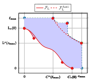
(a) Value functions for Problems (39) and (41).

(b) Value functions for Problems (40) and (42).

(c) Pareto and anti-Pareto frontier.

(d) Pareto and anti-Pareto frontier under additional regularity Assumptions 4-7.

Figure 2. An example of the possible aspects of the feasible region $\mathbf{F}$ (in light blue), the value functions $\mathrm{L}_{\star}$, $\mathrm{L}^{\star}$, $C_{\star}$, $C^{\star}$, and the Pareto and anti-Pareto frontier (in red) under Assumption 3.

The next two hypotheses on $C$ and $\mathrm{L}$ will imply that the Pareto frontier is connected.

Assumption 4.

If the cost $C$ has a local minimum (for the weak topology) at $\eta$, then $C(\eta)=0$ and $\eta$ is a global minimum of $C$.

Assumption 5.

If the loss $\mathrm{L}$ has a local minimum (for the weak topology) at $\eta$, then $\mathrm{L}(\eta)=0$ and $\eta$ is a global minimum of $\mathrm{L}$.

Under these hypotheses, the picture becomes much nicer, see Figure 2(d), where the only flat parts of the graphs of $C_{\star}$ and $\mathrm{L}_{\star}$ occur at zero cost or zero loss.

Proposition 5.5.

Under Assumption 3 and 4 the following properties hold:

1. The optimal cost $C_{\star}$ is decreasing on $[0,\mathrm{L}_{\star}(0)]$.

2. If $\eta$ solves Problem (40) for the loss $\ell\in[0,\mathrm{L}_{\star}(0)]$, then $\mathrm{L}(\eta)=\ell$ (that is, the constraint is binding). Moreover $\eta$ is Pareto optimal, and:

   (43) $$\mathrm{L}_{\star}(C_{\star}(\ell))=\ell.$$

3. The Pareto frontier is the graph of $C_{\star}$:

   (44) $$\mathcal{F}_{\mathrm{L}}=\{(C_{\star}(\ell),\ell)\,\colon\,\ell\in[0,\mathrm{L}_{\star}(0)]\}.$$

Similarly, under Assumptions 3 and 5, the following properties hold:

1. The optimal loss $\mathrm{L}_{\star}$ is decreasing on $[0,C_{\star}(0)]$.

2. If $\eta$ solves Problem (39) for the cost $c\in[0,C_{\star}(0)]$, then $C(\eta)=c$. Moreover $\eta$ is Pareto optimal, and $C_{\star}(\mathrm{L}_{\star}(c))=c$.

3. The Pareto frontier is the graph of $\mathrm{L}_{\star}$:

   (45) $$\mathcal{F}_{\mathrm{L}}=\{(c,\mathrm{L}_{\star}(c))\,\colon\,c\in[0,C_{\star}(0)]\}.$$

Finally, if Assumptions 4 and 5 hold, then $\mathrm{L}_{\star}$ is a continuous decreasing bijection of $[0,C_{\star}(0)]$ onto $[0,L^{\star}(0)]$ and $C_{\star}$ is the inverse bijection, and the Pareto frontier is compact and connected.

Proof.

We prove (i). Let $0\leq\ell<\ell^{\prime}\leq\mathrm{L}_{\star}(0)$, and let $\eta_{\star}$ be a solution of Problem (40):

(46) $$C(\eta_{\star})=C_{\star}(\ell)\quad\text{and}\quad\mathrm{L}(\eta_{\star})\leq\ell.$$

The set $\mathcal{O}=\{\eta\,\colon\,\mathrm{L}(\eta)<\ell^{\prime}\}$ is open and contains $\eta_{\star}$. Since $\mathrm{L}(\eta_{\star})<\mathrm{L}_{\star}(0)$, we get $C(\eta_{\star})>0$, so $\eta_{\star}$ is not a global minimum for $C$. By Assumption 4, it cannot be a local minimum for $C$, so $\mathcal{O}$ contains at least one point $\eta^{\prime}$ for which $C(\eta^{\prime})<C(\eta_{\star})$. Since $\eta^{\prime}\in\mathcal{O}$, we get $\mathrm{L}(\eta^{\prime})\leq\ell^{\prime}$, so that $C_{\star}(\ell^{\prime})\leq C(\eta^{\prime})<C(\eta_{\star})=C_{\star}(\ell)$. Since $\ell<\ell^{\prime}$ are arbitrary, $C_{\star}$ is decreasing on $[0,\mathrm{L}_{\star}(0)]$.

We now prove (ii). If the inequality in (46) was strict, that is $\mathrm{L}(\eta_{\star})<\ell$, then we would get a contradiction as $C(\eta_{\star})\geq C_{\star}(\mathrm{L}(\eta_{\star}))>C_{\star}(\ell)=C(\eta_{\star})$. Therefore any solution $\eta_{\star}$ of (40) satisfies $\mathrm{L}(\eta_{\star})=\ell$, and in particular $C_{\star}(\mathrm{L}(\eta_{\star}))=C_{\star}(\ell)=C(\eta_{\star})$. This implies in turn that $\eta_{\star}$ also solves (39): if $\eta$ satisfies $\mathrm{L}(\eta)<\mathrm{L}(\eta_{\star})$, then using the definition of $C_{\star}$, the fact that it decreases, and the definition of $\eta_{\star}$, we get:

$$C(\eta)\geq C_{\star}(\mathrm{L}(\eta))>C_{\star}(\mathrm{L}(\eta_{\star}))=C(\eta_{\star}).$$

By contraposition, we have $\mathrm{L}(\eta)\geq\mathrm{L}(\eta_{\star})$ for any $\eta$ such that $C(\eta)\leq C(\eta_{\star})$, proving that $\eta_{\star}$ is also a solution of (39) with $c=C(\eta_{*})$. By Point (i) of Proposition 5.4, $\eta_{\star}$ is Pareto optimal. Therefore $(C(\eta_{\star}),\mathrm{L}(\eta_{\star}))=(C_{\star}(\ell),\ell)$ belongs to the Pareto frontier. Using Point (ii) of Proposition 5.4, we deduce that $\ell=\mathrm{L}_{\star}(C_{\star}(\ell))$.

To prove Point (iii), note that Equation (43) shows that, if $c=C_{\star}(\ell)$ for $\ell\in[0,\mathrm{L}_{\star}(0)]$, then $\ell=\mathrm{L}_{\star}(c)$. Use Point (ii) and (iii) of Proposition 5.4, to get that $\mathcal{F}_{\mathrm{L}}=\{(c,\ell)\,\colon\,c=C_{\star}(\ell),\,\ell\in[0,\mathrm{L}_{\star}(0)]\}$.

The claims (iv), (v) and (vi) are proved in the same way, exchanging the roles of $\mathrm{L}$ and $C$.

To conclude the proof, it remains to check that $C_{\star}$ and $\mathrm{L}_{\star}$ are continuous under Assumptions 3, 4 and 5. We deduce from Point (ii) and Proposition 5.3 that $[0,\mathrm{L}_{\star}(0)]$ is in the range of $\mathrm{L}_{\star}$. Since $\mathrm{L}_{\star}$ is decreasing, thanks to Point (iv) and $\mathrm{L}_{\star}(C_{\star}(0))=0$, see Proposition 5.4 (iii), we get that $\mathrm{L}_{\star}$ is continuous and decreasing on $[0,\mathrm{L}_{\star}(0)]$, and thus one-to-one from $[0,C_{\star}(0)]$ onto $[0,\mathrm{L}^{\star}(0)]$. Then use (43) to get that $C_{\star}$ is its inverse bijection. The continuity of $\mathrm{L}_{\star}$ and (45) implies that $\mathcal{F}_{\mathrm{L}}$ is compact and connected. ∎

Finally, let us check that Assumptions 4 and 5 hold under very simple assumptions, which are in particular satisfied by the cost functions $C_{\mathrm{uni}}$ and $C_{\mathrm{aff}}$ and the loss functions $R_{e}$ and $\mathfrak{I}$ (recall from Propositions 4.1 and 4.5 that $R_{e}$ and $\mathfrak{I}$ are sub-homogeneous).

Lemma 5.6.

Suppose Assumption 3 holds. If the cost function $C$ is decreasing, then Assumption 4 holds and $\mathrm{L}_{\star}(0)=\ell_{\max}$. If the loss function $\mathrm{L}$ is sub-homogeneous, then Assumption 5 holds.

Proof.

Let $\eta\in\Delta$. If $C$ has a local minimum at $\eta$, then, as $C$ is non-increasing, for $\varepsilon>0$ small enough, we get that $C(\eta)\geq C(\eta+\varepsilon(1-\eta))\geq C(\eta)$. If $C$ is decreasing, this is only possible if $\eta=1$ almost surely, so that $\eta$ is a global minimum of $C$. This also gives $\mathrm{L}_{\star}(0)=\ell_{\max}$. Similarly if $\mathrm{L}$ has a local minimum at $\eta$, then for $\varepsilon>0$ small enough $\mathrm{L}(\eta)\leq\mathrm{L}((1-\varepsilon)\eta)\leq(1-\varepsilon)\mathrm{L}(\eta)$, so $\mathrm{L}(\eta)=0$ and $\eta$ is a global minimum of $\mathrm{L}$. ∎

Corollary 5.7.

Suppose that Assumptions 3, 4 and 5 hold. The set of Pareto optimal strategies $\mathcal{P}_{\mathrm{L}}$ is compact (for the weak topology).

Proof.

Since $\mathrm{L}_{\star}$ is continuous thanks to Proposition 5.5, we deduce that $\mathcal{F}_{\mathrm{L}}$, which is given by (45), is compact and thus closed. Since $\mathcal{P}_{\mathrm{L}}=f^{-1}(\mathcal{F}_{\mathrm{L}})$, where the function $f=(C,\mathrm{L})$ defined on $\Delta$ is continuous, we deduce that $\mathcal{P}_{\mathrm{L}}$ is closed and thus compact as $\Delta$ is compact. ∎

5.3. On the anti-Pareto frontier

5.3.1. The general setting

Letting $C^{\prime}(\eta)=\ell_{\max}-\mathrm{L}(\eta)$ and $\mathrm{L}^{\prime}(\eta)=c_{\max}-C(\eta)$, it is easy to see that:

$$C_{\star}^{\prime}(c)=\ell_{\max}-\mathrm{L}^{\star}(c_{\max}-c)\quad\text{and}\quad\mathrm{L}_{\star}^{\prime}(\ell)=c_{\max}-C^{\star}(\ell_{\max}-\ell),$$

so that Proposition 5.5 may be applied to the cost function $C^{\prime}$ and the loss function $\mathrm{L}^{\prime}$ to yield the following result.

Proposition 5.8 (Single-objective and bi-objective problems for the anti-Pareto strategies).

Suppose Assumption 3 holds.

1. If $\eta^{\star}$ is anti-Pareto optimal, then $\eta^{\star}$ is a solution of (41) for the cost $c=C(\eta^{\star})$, and a solution of (42) for the loss $\ell=\mathrm{L}(\eta^{\star})$. Conversely, if $\eta^{\star}$ is a solution to both problems (41) and (42) for some values $c$ and $\ell$, then $\eta^{\star}$ is anti-Pareto optimal.

2. The anti-Pareto frontier is the intersection of the graphs of $C^{\star}$ and $\mathrm{L}^{\star}$:

   $$\mathcal{F}_{\mathrm{L}}^{\mathrm{Anti}}=\{(c,\ell)\in[0,c_{\max}]\times[0,\ell_{\max}]\,\colon\,c=C^{\star}(\ell)\text{ and }\ell=\mathrm{L}^{\star}(c)\}.$$

3. The points $(C^{\star}(\ell_{\max}),\ell_{\max})$ and $(c_{\max},\mathrm{L}^{\star}(c_{\max}))$ both belong to the anti-Pareto frontier, and we have $C^{\star}(\mathrm{L}^{\star}(c_{\max}))=c_{\max}$ and $\mathrm{L}^{\star}(C^{\star}(\ell_{\max}))=\ell_{\max}$. Moreover, we also have $C^{\star}(\ell)=c_{\max}$ for $\ell\in[0,\mathrm{L}^{\star}(c_{\max})]$, and $\mathrm{L}^{\star}(c)=\ell_{\max}$ for $c\in[0,C^{\star}(\ell_{\max})]$.

The following additional hypotheses rule out the occurrence of flat parts in the anti-Pareto frontier.

Assumption 6.

If the cost $C$ has a local maximum at $\eta$ (for the weak topology), then $C(\eta)=c_{\max}$ and $\eta$ is a global maximum of $C$.

Assumption 7.

If the loss $\mathrm{L}$ has a local maximum at $\eta$ (for the weak topology), then $\mathrm{L}(\eta)=\ell_{\max}$ and $\eta$ is a global maximum of $\mathrm{L}$.

The following result is now a consequence of Proposition 5.5 and Corollary 5.7 applied to the loss function $\mathrm{L}^{\prime}$ and cost function $C^{\prime}$.

Proposition 5.9.

Under Assumption 3 and 6 the following properties hold:

1. The optimal cost $C^{\star}$ is decreasing on $[C^{\star}(\ell_{\max}),c_{\max}]$.

2. If $\eta$ solves Problem (42) for the loss $\ell\in[\mathrm{L}^{\star}(c_{\max}),\ell_{\max}]$, then $\mathrm{L}(\eta)=\ell$ (that is, the constraint is binding). Moreover $\eta$ is anti-Pareto optimal, and $\mathrm{L}^{\star}(C^{\star}(\ell))=\ell$.

3. The anti-Pareto frontier is the graph of $C^{\star}$:

   (47) $$\mathcal{F}_{\mathrm{L}}^{\mathrm{Anti}}=\{(C^{\star}(\ell),\ell)\,\colon\,\ell\in[\mathrm{L}^{\star}(c_{\max}),\ell_{\max}]\}.$$

Similarly, under Assumptions 3 and 7, the following properties hold:

1. The optimal loss $\mathrm{L}^{\star}$ is decreasing on $[\mathrm{L}^{\star}(c_{\max}),\ell_{\max}]$.

2. If $\eta$ solves Problem (41) for the cost $c\in[C^{\star}(\ell_{\max}),c_{\max}]$, then $C(\eta)=c$. Moreover $\eta$ is anti-Pareto optimal, and $C^{\star}(\mathrm{L}^{\star}(c))=c$.

3. The anti-Pareto frontier is the graph of $\mathrm{L}^{\star}$:

   (48) $$\mathcal{F}_{\mathrm{L}}^{\mathrm{Anti}}=\{(c,\mathrm{L}^{\star}(c))\,\colon\,c\in[C^{\star}(\ell_{\max}),c_{\max}]\}.$$

Finally, if Assumptions 3, 6 and 7 hold, then $\mathrm{L}^{\star}$ is a continuous decreasing bijection of $[C^{\star}(\ell_{\max}),c_{\max}]$ onto $[\mathrm{L}^{\star}(c_{\max}),\ell_{\max}]$, $C^{\star}$ is the inverse bijection, and the anti-Pareto frontier is compact and connected. Furthermore, the set of anti-Pareto optimal strategies $\mathcal{P}_{\mathrm{L}}^{\mathrm{Anti}}$ is compact (for the weak topology).

The following result is similar to the first part of Lemma 5.6.

Lemma 5.10.

Suppose Assumption 3 holds. If the cost function $C$ is decreasing, then Assumption 6 holds and $\mathrm{L}^{\star}(c_{\max})=0$.

Proof.

Let $\eta\in\Delta$ and $\varepsilon\in(0,1)$. Since $C$ is decreasing, $C((1-\varepsilon)\eta)\geq C(\eta)$, with equality if and only if $\eta=0$ $\mu$-almost surely. Therefore the only local maximum of $C$ is $\eta=0$, and it is a global maximum. Since $C(\eta)=c_{\max}$ implies that $\eta=0$ $\mu$-almost surely, we also get that $\mathrm{L}^{\star}(c_{\max})=\mathrm{L}(0)=0$. ∎

5.3.2. The particular case of the kernel and SIS models

We show that, under an irreducibility hypothesis on the kernel, Assumption 7 holds for the loss functions $R_{e}$ and $\mathfrak{J}$. The reducible case is more delicate and it is studied in more details in [8] for the loss function $\mathrm{L}=R_{e}$; in particular Assumption 7 may not hold and the anti-Pareto frontier may not be connected.

Let us recall some notation. Let $\mathrm{k}$ be a kernel with finite double norm. For $A,B\in\mathscr{F}$, we write $A\subset B$ a.s. if $\mu(B\cap A^{c})=0$ and $A=B$ a.s. if $A\subset B$ a.s. and $B\subset A$ a.s. For $A,B\in\mathscr{F}$, $x\in\Omega$ and a kernel $\mathrm{k}$, we simply write $\mathrm{k}(x,A)=\int_{A}\mathrm{k}(x,y)\,\mu(\mathrm{d}y)$, $\mathrm{k}(B,x)=\int_{B}\mathrm{k}(z,x)\,\mu(\mathrm{d}z)$ and:

$$\mathrm{k}(B,A)=\int_{B\times A}\mathrm{k}(z,y)\,\mu(\mathrm{d}z)\mu(\mathrm{d}y).$$

A set $A\subset\mathscr{F}$ is $\mathrm{k}$-invariant if $\mathrm{k}(A^{c},A)=0$. (Notice that if $A$ is $\mathrm{k}$-invariant, then $L^{p}(A,\mu)$ is an invariant closed subspace for $T_{\mathrm{k}}$, seen as an operator on $L^{p}(\Omega,\mu)$.) A kernel $\mathrm{k}$ is irreducible (or connected) if any $\mathrm{k}$-invariant set $A$ is such that a.s. $A=\emptyset$ or a.s. $A=\Omega$. Define $\{\mathrm{k}\equiv 0\}$ as $\{x\in\Omega\,\colon\,\mathrm{k}(x,\Omega)+\mathrm{k}(\Omega,x)=0\}$, so that $\mathrm{k}(A,\Omega)+\mathrm{k}(\Omega,A)=0$ implies that a.s. $A\subset\{\mathrm{k}\equiv 0\}$. A kernel $\mathrm{k}$ is quasi-irreducible if the restriction of $\mathrm{k}$ to $\{\mathrm{k}\equiv 0\}^{c}$ is irreducible, that is if any $\mathrm{k}$-invariant set $A$ is such that $A\subset\{\mathrm{k}\equiv 0\}$ a.s. or $A^{c}\subset\{\mathrm{k}\equiv 0\}$ a.s. Notice the definition of the quasi-irreducibility from [3, Definition 2.11] is slightly stronger as it uses a topology on $\Omega$.

Lemma 5.11.

Consider the kernel model $\mathrm{Param}=[(\Omega,\mathscr{F},\mu),\mathrm{k}]$ under Assumption 1. If $\mathrm{k}$ is quasi-irreducible, then Assumption 7 holds for $\mathrm{L}=R_{e}[\mathrm{k}]$, and $C^{\star}(\ell_{\max})=C(\mathds{1}_{\{\mathrm{k}\equiv 0\}^{c}})$ (which is 0 if $\mathrm{k}$ is irreducible).

Proof.

The quasi-irreducible case can easily be deduced from the irreducible case, so we assume that $\mathrm{k}$ is irreducible. In particular, we have $\mathrm{k}(\Omega,y)>0$ almost surely. Let $\eta\in\Delta$ be a local maximum of $R_{e}$ on $\Delta$; we want to show that it is also a global maximum.

Suppose first that $\inf\eta>0$. Then $\mathrm{k}\eta$ is irreducible with finite double norm. According [41, Theorem V.6.6 and Example V.6.5.b], the eigenspace of $T_{\mathrm{k}\eta}$ associated to $R_{e}(\eta)$ is one-dimensional and it is spanned by a vector $v_{\mathrm{d}}$ such that $v_{\mathrm{d}}>0$ almost surely, and the corresponding left eigenvector associated to $R_{e}(\eta)$, say $v_{\mathrm{g}}$, can be chosen such that $\langle v_{\mathrm{g}},v_{\mathrm{d}}\rangle=1$ and $v_{\mathrm{g}}>0$ almost surely. According to [31, Theorem 2.6], applied to $L_{0}=T_{\mathrm{k}\eta}$ and $L=T_{\mathrm{k}(\eta+\varepsilon(1-\eta))}$, we have, using that $\lVert L_{0}-L\rVert=O(\varepsilon)$ thanks to (12):

$$R_{e}(\eta+\varepsilon(1-\eta))=R_{e}(\eta)+\varepsilon\langle v_{\mathrm{g}},T_{\mathrm{k}(1-\eta)}v_{\mathrm{d}}\rangle+O(\varepsilon^{2}).$$

Since $R_{e}$ has a local maximum at $\eta$, the first order term on the right hand side vanishes, so $v_{\mathrm{g}}(x)\mathrm{k}(x,y)(1-\eta(y))v_{\mathrm{d}}(y)=0$ for $\mu$ almost all $x$ and $y$. Since $v_{\mathrm{g}}$ and $v_{\mathrm{d}}$ are positive almost surely and $\mathrm{k}$ is irreducible, we get that $\mathrm{k}(\Omega,y)(1-\eta(y))=0$ almost surely and thus $\eta(y)=1$ almost surely. Therefore $\eta=\mathds{1}$, which is a global maximum for $R_{e}$.

Finally, suppose that $\inf\eta=0$. Let $\mathcal{O}$ be an open subset of $\Delta$ on which $R_{e}\leq R_{e}(\eta)$ and with $\eta\in\mathcal{O}$. For $\varepsilon>0$ small enough, the strategy $\eta_{\varepsilon}=\eta+\varepsilon(1-\eta)$ belongs to $\mathcal{O}$ and satisfies $R_{e}(\eta)\leq R_{e}(\eta_{\varepsilon})\leq R_{e}(\eta)$ (where the first inequality comes from the fact that $R_{e}$ is non-decreasing). Therefore $\eta_{\varepsilon}$ is a local maximum, and thus $\eta_{\varepsilon}=\mathds{1}$ almost surely. This readily implies that $\eta=\mathds{1}$ almost surely.

We deduce that if $\eta$ is a local maximum, then $\eta=1$ almost surely. Thus $\eta$ is a global maximum and $C^{\star}(\ell_{\max})=C(\mathds{1})=0$. This ends the proof. ∎

Lemma 5.12.

Consider the SIS model $\mathrm{Param}=[(\Omega,\mathscr{F},\mu),k,\gamma]$ under Assumption 2. If $k$ is quasi-irreducible, then Assumption 7 holds for $\mathrm{L}=\mathfrak{I}$ and $C^{\star}(\ell_{\max})=C(\mathds{1}_{\{\mathrm{k}\equiv 0\}^{c}})$ (which is 0 if $k$ is irreducible).

Proof.

The quasi-irreducible case can easily be deduced from the irreducible case, so we assume that $k$ is irreducible.

Set $\mathrm{k}=k/\gamma$. Suppose that $\mathfrak{I}$ has a local maximum at some $\eta\in\Delta$. For $\varepsilon\in(0,1)$, the kernel $\mathrm{k}{\eta_{\varepsilon}}$, with $\eta_{\varepsilon}=\eta+\varepsilon(1-\eta)$, is irreducible (with finite double norm) since $k$ is irreducible and $\gamma$ is positive and bounded. We have that for $\varepsilon>0$ small enough:

$$\mathfrak{I}(\eta)\geq\mathfrak{I}(\eta_{\varepsilon})=\int_{\Omega}\mathfrak{g}_{\eta_{\varepsilon}}\,\eta_{\varepsilon}\,\mathrm{d}\mu\geq\int_{\Omega}\mathfrak{g}_{\eta_{\varepsilon}}\,\eta\,\mathrm{d}\mu\geq\int_{\Omega}\mathfrak{g}_{\eta}\,\eta\,\mathrm{d}\mu=\mathfrak{I}(\eta),$$

where we used that $\eta\leq\eta_{\varepsilon}$ and $0\leq\mathfrak{g}_{\eta}\leq\mathfrak{g}_{\eta_{\varepsilon}}$, see (33). Therefore all these quantities are equal. Since the equilibrium $\mathfrak{g}_{\eta_{\varepsilon}}$ is $\mu$-a.e. positive thanks to [7, Remark 4.11] as $\mathrm{k}\eta_{\varepsilon}$ is irreducible, we must have $\eta_{\varepsilon}=\eta$ a.s, which is only possible if $\eta=1$ almost surely.

Since $\mathfrak{I}(\mathds{1})>\mathfrak{I}(\eta)$ for any $\eta\neq\mathds{1}$, we also get $C^{\star}(\ell_{\max})=0$, with $\ell_{\max}=\mathfrak{I}(\mathds{1})=\int_{\Omega}\mathfrak{g}\,\mathrm{d}\mu$. ∎

6. Miscellaneous properties for set of outcomes and the Pareto frontier

We prove results concerning the feasible region, the stability of the Pareto frontier and its geometry.

6.1. No holes in the feasible region

We check there is no hole in the feasible region.

Proposition 6.1.

Suppose that Assumption 3 holds. The feasible region $\mathbf{F}$ is compact, path connected, and its complement is connected in $\mathbb{R}^{2}$. It is the whole region between the graphs of the one-dimensional value functions:

$$\mathbf{F} =\{(c,\ell)\in\mathbb{R}^{2}\,\colon\,0\leq c\leq c_{\max},\,\mathrm{L}_{\star}(c)\leq\ell\leq\mathrm{L}^{\star}(c)\}$$

$$=\{(c,\ell)\in\mathbb{R}^{2}\,\colon\,0\leq\ell\leq\ell_{\max},\,C_{\star}(\ell)\leq c\leq C^{\star}(\ell)\}.$$

Proof.

The region $\mathbf{F}$ is compact and path-connected as a continuous image by $(C,\mathrm{L})$ of the compact, path-connected set $\Delta$.

By symmetry, it is enough to prove that $\mathbf{F}$ is equal to $F_{1}=\{(c,\ell)\in\mathbb{R}^{2}\,\colon\,0\leq c\leq c_{\max},\,\mathrm{L}_{\star}(c)\leq\ell\leq\mathrm{L}^{\star}(c)\}$. Let $(c,\ell)\in\mathbf{F}$ and $\eta\in\Delta$ be such that $(c,\ell)=(C(\eta),\mathrm{L}(\eta))$. By definition of $\mathrm{L}_{\star}$ and $\mathrm{L}^{\star}$, we have: $\mathrm{L}_{\star}(c)=\mathrm{L}_{\star}(C(\eta))\leq\mathrm{L}(\eta)\leq\mathrm{L}^{\star}(C(\eta))=\mathrm{L}^{\star}(c)$. We deduce that $(c,\ell)\in F_{1}$.

Let us now prove that $F_{1}\subset\mathbf{F}$. Let us first consider a point of the form $(c,\mathrm{L}_{\star}(c))$, where $0\leq c\leq c_{\max}$. By definition, there exists $\eta$ such that $C(\eta)\leq c$ and $\mathrm{L}(\eta)=\mathrm{L}_{\star}(c)$. Let $\eta_{t}=t\eta$. The map $t\mapsto C(\eta_{t})$ is continuous from $[0,1]$ to $[C(\eta),c_{\max}]$, and $c\in[C(\eta),c_{\max}]$, so there exists $s$ such that $C(\eta_{s})=c$. Since $\mathrm{L}$ is non-decreasing, $\mathrm{L}(\eta_{s})\leq\mathrm{L}(\eta)$. By definition of $\mathrm{L}_{\star}(c)$, $\mathrm{L}(\eta_{s})\geq\mathrm{L}_{\star}(c)$. Therefore $(c,\mathrm{L}_{\star}(c))=(C(\eta_{s}),\mathrm{L}(\eta_{s}))$ belongs to $\mathbf{F}$. Similarly the graphs of $C_{\star}$, $C^{\star}$ and $\mathrm{L}^{\star}$ are also included in $\mathbf{F}$.

So, it is enough to check that, if $A=(c,\ell)$ is in $F_{1}$, with $c\in(0,c_{\max})$ and $\ell\in(\mathrm{L}_{\star}(c),\mathrm{L}^{\star}(c))$, then $A$ belongs to $\mathbf{F}$. We shall assume that $A\not\in\mathbf{F}$ and derive a contradiction by building a loop in $\mathbf{F}$ that encloses $A$ and which can be continuously contracted into a point in $\mathbf{F}$.

Since $\mathrm{L}_{\star}(c)<\ell<\mathrm{L}^{\star}(c)$, there exist $\eta_{\text{\tiny SO}}$ and $\eta_{\text{\tiny NE}}$ such that:

$$C(\eta_{\text{\tiny SO}})\leq c,\quad\mathrm{L}(\eta_{\text{\tiny SO}})<\ell,\quad C(\eta_{\text{\tiny NE}})\geq c\quad\text{and}\quad\mathrm{L}(\eta_{\text{\tiny NE}})>\ell.$$

We concatenate the four paths defined for $u\in[0,1]$:

$$u\mapsto u\eta_{\text{\tiny SO}},\quad u\mapsto(1-u)\eta_{\text{\tiny SO}}+u,\quad u\mapsto(1-u)+u\eta_{\text{\tiny NE}}\quad\text{and}\quad u\mapsto(1-u)\eta_{\text{\tiny NE}},$$

to obtain a continuous loop $(\eta_{t},t\in[0,4])$ from $[0,4]$ to $\Delta$, such that:

$$\eta_{0}=\eta_{4}=0,\quad\eta_{1}=\eta_{\text{\tiny SO}},\quad\eta_{2}=1\quad\text{and}\quad\eta_{3}=\eta_{\text{\tiny NE}}.$$

We now define a continuous family of loops $(\gamma_{s},s\in[0,1])$ in $\mathbb{R}^{2}$ by

$$\gamma_{s}(t)=(C(s\eta_{t}),\mathrm{L}(s\eta_{t}),t\in[0,4]).$$

By definition, for all $s\in[0,1]$, $\gamma_{s}$ is a continuous loop in $F$. Since $A=(c,\ell)\notin\mathbf{F}$, the loops $\gamma_{s}$ do not contain $A$, so the winding number $W(\gamma_{s},A)$ is well-defined (see for example [26, Definition 6.1]). As $A\not\in\mathbf{F}$, we get that $\gamma_{s}$ is a continuous deformation in $\mathbb{R}^{2}\setminus\{A\}$ from $\gamma_{1}$ to $\gamma_{0}$. Thanks to [26, Theorem 6.5], this implies that $W(\gamma_{s},A)$ does not depend on $s\in[0,1]$.

For $s=0$, the loop degenerates to the single point $(C(0),0)$ so the winding number is $0$. For $s=1$, let us check that the winding number is $1$, which will provide the contradiction. To do this, we compare $\gamma_{1}$ with a simpler loop $\delta$ defined by:

$$\delta(0)=\delta(4)=(c_{\max},0),\quad\delta(1)=(0,0),\quad\delta(2)=(0,\ell_{\max})\quad\text{and}\quad\delta(3)=(c_{\max},\ell_{\max}),$$

and by linear interpolation for non integer values of $t$: in other words, $\delta$ runs around the perimeter of the axis-aligned rectangle with corners $(0,0)$ and $(c_{\max},\ell_{\max})$. Clearly, we have $W(\delta,A)=1$.

Let $M_{t}$, $N_{t}$ denote $\gamma_{1}(t)$ and $\delta(t)$ respectively. For $t\in[0,1]$, we have $N_{t}=((1-t)c_{\max},0)$, so the second coordinate of $\overrightarrow{AN_{t}}$ is non-positive. On the other hand $\mathrm{L}(t\eta_{\text{\tiny SO}})\leq\mathrm{L}(\eta_{\text{\tiny SO}})<\ell$, so the second coordinate of $\overrightarrow{AM_{t}}$ is negative. Therefore the two vectors $\overrightarrow{AN_{t}}$ and $\overrightarrow{AM_{t}}$ cannot point in opposite directions. Similar considerations for the other values of $t\in[1,4]$ show that $\overrightarrow{AN_{t}}$ and $\overrightarrow{AM_{t}}$ never point in opposite directions. By [26, Theorem 6.1], the winding numbers $W(\gamma_{1},A)$ and $W(\delta,A)$ are equal, and thus $W(\gamma_{1},A)=1$.

This gives that $A\in\mathbf{F}$ by contradiction, and thus $F_{1}\subset\mathbf{F}$.

Finally, it is easy to check that $F_{1}$ has a connected complement, because $F_{1}$ is bounded, and all the points in $F_{1}^{c}$ can reach infinity by a straight line: for example, if $\ell>\mathrm{L}^{\star}(c)$, then the half-line $\{(c,\ell^{\prime}),\ell^{\prime}\geq\ell\}$ is in $F_{1}^{c}$. ∎

6.2. Stability

We can consider the stability of the Pareto frontier and the set of Pareto optima. Recall that, thanks to (45), the graph $\{(c,\mathrm{L}_{\star}(c))\,\colon\,c\in[0,c_{\max}]\}$ of $\mathrm{L}_{\star}$ is the union of the Pareto frontier and the straight line joining $(0,C_{\star}(0))$ to $(0,c_{\max})$ and can thus be seen as an extended Pareto frontier. The proof of the following proposition is immediate. It implies in particular the convergence of the extended Pareto frontier. This result can also easily be adapted to the anti-Pareto frontier.

Proposition 6.2.

Let $C$ be a cost function and $(\mathrm{L}^{(n)},n\in\mathbb{N})$ a sequence of loss functions converging uniformly on $\Delta$ to a loss function $\mathrm{L}$. Assume that Assumptions 3, 4 and 5 hold for the cost $C$ and the loss functions $\mathrm{L}^{(n)}$, $n\in\mathbb{N}$, and $\mathrm{L}$. Then $\mathrm{L}_{\star}^{(n)}$ converges uniformly to $\mathrm{L}_{\star}$. Let $\eta\in\Delta$ be the weak limit of a sequence $(\eta_{n},n\in\mathbb{N})$ of Pareto optima, that is $\eta_{n}\in\mathcal{P}_{\mathrm{L}^{(n)}}$ for all $n\in\mathbb{N}$. If $C(\eta)\leq C_{\star}(0)$, then we have $\eta\in\mathcal{P}_{\mathrm{L}}$.

Remark 6.3 (On the continuity of the Pareto Frontier).

It might happen that some elements of $\mathcal{P}_{\mathrm{L}}$ are not weak limit of sequence of elements of $\mathcal{P}_{\mathrm{L}^{(n)}}$; see [9] for such discontinuity. It might also happen that a sequence $(\eta_{n},\,n\in\mathbb{N})$ such that $\eta_{n}\in\mathcal{P}_{\mathrm{L}^{(n)}}$ and $\mathrm{L}^{(n)}(\eta_{n})>0$ converges to some $\eta$ that does not belong to $\mathcal{P}_{\mathrm{L}}$ if $\mathrm{L}(\eta)=0$. In particular, in this case, ${C_{\star}}_{,\mathrm{L}^{(n)}}(0)$ does not converge to ${C_{\star}}_{,\mathrm{L}}(0)$, where ${C_{\star}}_{,\mathrm{L}^{\prime}}$ is the value function $C_{\star}$ associated to the loss $\mathrm{L}^{\prime}$. This situation is represented in Figure 3. In Figure 3(a), we have plotted a perturbation $\mathrm{k}_{\varepsilon}=\mathrm{k}+\varepsilon\sum_{n\in\mathbb{N}^{\star}}\mathds{1}_{I_{n}\times I_{n}}$ of the multipartite kernel $\mathrm{k}$ defined in Example 1.7 for $\varepsilon>0$ small. According to Proposition 4.3, $R_{e}[\mathrm{k}_{\varepsilon}]$ converges uniformly to $R_{e}[\mathrm{k}]$ when $\varepsilon$ vanishes. However, the Pareto optimal strategies for $\mathrm{k}_{\varepsilon}$ that cost more than $1/2$ do not converge to some Pareto optimal strategies for $\mathrm{k}$. This can be seen in Figure 3(b), where the Pareto frontier of $\mathrm{k}_{\varepsilon}$ (in blue) corresponding to costs larger than 1/2 does not have a counterpart in the Pareto frontier of $\mathrm{k}$ (in red).

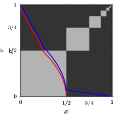
(a) Grayplot of the kernel $\mathrm{k}_{\varepsilon}$, with $\Omega=[0,1]$ and $\mu$ the Lebesgue measure ($\mathrm{k}_{\varepsilon}$ is equal to the constant $\kappa>0$ on the black zone and to $\varepsilon$ on the gray zone, with $\varepsilon>0$ small).

(b) In red, the Pareto frontier of the kernel $\mathrm{k}$ represented in Figure 1(a) compared to the Pareto frontier of the kernel $\mathrm{k}_{\varepsilon}$ in blue.

Figure 3. On the stability of the Pareto frontier

6.3. Geometric properties

If the cost function is affine, then there is a nice geometric property of the Pareto frontier.

Lemma 6.4.

Suppose that Assumption 3 holds, the cost function is affine (i.e., $C=C_{\mathrm{aff}}$ given by (35)) and the loss function $\mathrm{L}$ is sub-homogeneous. Then, we have $\mathrm{L}_{\star}(\theta c+(1-\theta)c_{\max})\leq\theta\mathrm{L}_{\star}(c)$ for all $c\in[0,c_{\max}]$ and $\theta\in[0,1]$.

Remark 6.5.

Geometrically, Lemma 6.4 means that the graph of the loss $\mathrm{L}_{\star}\,\colon\,[0,c_{\max}]\to[0,\ell_{\max}]$ is below its chords with end point $(1,\mathrm{L}_{\star}(\mathds{1}))=(1,0)$. See Figures 1(b) for a typical representation of the Pareto frontier (red solid line).

Proof.

Let $c\in[0,c_{\max}]$ and $\theta\in[0,1]$. Thanks to Lemma 5.6, Assumption 5 holds. Thus, thanks to Proposition 5.5 (iv), there exists $\eta\in\mathcal{P}_{\mathrm{L}}$ with cost $C(\eta)=c$ and thus $\mathrm{L}(\eta)=\mathrm{L}_{\star}(c)$. Since $C$ is affine, we have:

$$C(\theta\eta)=\theta C(\eta)+(1-\theta)c_{\max}\leq\theta c+(1-\theta)c_{\max}.$$

Therefore, $\theta\eta$ is admissible for Problem (39) with cost constraint $C(\cdot)\leq\theta c+(1-\theta)c_{\max}$. This implies that $\mathrm{L}_{\star}(\theta c+(1-\theta)c_{\max})\leq\mathrm{L}(\theta\eta)\leq\theta\mathrm{L}_{\star}(c)$, thanks to the sub-homogeneity of the loss function $\mathrm{L}$. ∎

In some case, we shall prove that the considered loss function is convex (which in turn implies Assumption 5). In this case, choosing a convex cost function implies that Assumption 4 holds and the Pareto frontier is convex. A similar result holds in the concave case. We provide a short proof of this result.

Proposition 6.6.

Suppose that Assumption 3 holds. If the cost function $C$ and the loss function $\mathrm{L}$ are convex, then the functions $C_{\star}$ and $\mathrm{L}_{\star}$ are convex. If the cost function $C$ and the loss function $\mathrm{L}$ are concave, then the functions $C^{\star}$ and $\mathrm{L}^{\star}$ are convex.

Proof.

Let $\ell_{0},\ell_{1}\in[0,\ell_{\max}]$. By Proposition 5.3, there exist $\eta_{0}$, $\eta_{1}$ such that $\mathrm{L}(\eta_{i})\leq\ell_{i}$ and $C(\eta_{i})=C_{\star}(\ell_{i})$ for $i\in\{0,1\}$. For $\theta\in[0,1]$, let $\ell=(1-\theta)\ell_{0}+\theta\ell_{1}$. Since $C$ and $\mathrm{L}$ are assumed to be convex, $\eta=(1-\theta)\eta_{0}+\theta\eta_{1}$ satisfies:

$$C(\eta)\leq(1-\theta)C_{\star}(\ell_{0})+\theta C_{\star}(\ell_{1})\quad\text{and}\quad\mathrm{L}(\eta)\leq(1-\theta)\ell_{0}+\theta\ell_{1}.$$

Therefore, we get that $C_{\star}((1-\theta)\ell_{0}+\theta\ell_{1})\leq C(\eta)\leq(1-\theta)C_{\star}(\ell_{0})+\theta C_{\star}(\ell_{1})$, and $C_{\star}$ is convex. The proof of the convexity of $\mathrm{L}_{\star}$ is similar. The concave case is also similar. ∎

7. Equivalence of models by coupling

Even if in full generality, the cost function could also be treated as a parameter, we shall for simplicity consider only the uniform cost $C_{\mathrm{uni}}$ given by (36) in this section. (The interested reader can use Remark 5.2 for a first generalization to the affine cost function given by (35).)

7.1. Motivation

The aim of this section is to provide examples of different set of parameters for which two kernel or SIS models are “equivalent”, in the intuitive sense that their Pareto frontiers are the same (as subsets of $\mathbb{R}_{+}^{2}$), and it is possible to map nicely the Pareto optima from one model to the another. In Section 7.4, we present an example where discrete models can be represented as a continuous models and an example based on measure preserving transformation in the spirit of the graphon theory. We shall consider the two families of models:

• the kernel model characterized by $\mathrm{Param}=[(\Omega,\mathscr{F},\mu),\mathrm{k}]$, with Assumption 1 fulfilled, and loss function $\mathrm{L}=R_{e}$;

• the SIS model characterized by $\mathrm{Param}=[(\Omega,\mathscr{F},\mu),k,\gamma]$, with Assumption 2 fulfilled, and loss function $\mathrm{L}\in\{R_{e},\mathfrak{I}\}$;

where $(\Omega,\mathscr{F},\mu)$ is a probability space, $\mathrm{k}$ and $k$ are non-negative kernels on $\Omega$ and $\gamma$ is a non-negative function on $\Omega$.

In order to emphasize the dependence of a quantity $H$ on the parameters $\mathrm{Param}$ of the model, we shall write $H[\mathrm{Param}]$ for $H$. For example we write: $\Delta[\mathrm{Param}]$ for the set of functions $\{\eta\in\mathscr{L}^{\infty}(\Omega,\mathscr{F})\,\colon\,1\geq\eta\geq 0\}$, which clearly depends on the parameters $\mathrm{Param}$; and the effective reproduction function $R_{e}[\mathrm{Param}]$. For example, under Assumption 2, we have the equality of the following functions: $R_{e}[(\Omega,\mathscr{F},\mu),k,\gamma]=R_{e}[(\Omega,\mathscr{F},\mu),k/\gamma,1]=R_{e}[(\Omega,\mathscr{F},\mu),k/\gamma]$, where for the last equality the left hand-side refers to the SIS model and the right hand-side refers to the kernel model (where Assumption 1 holds as a consequence of Assumption 2). Using (29) if $\inf\gamma>0$ (see [8, Section 3] for details and more general results), then we also have $R_{e}[(\Omega,\mathscr{F},\mu),k/\gamma]=R_{e}[(\Omega,\mathscr{F},\mu),\gamma^{-1}k]$.

7.2. On measurability

Let us recall some well-known facts on measurability. Let $(E,\mathscr{E})$ and $(E^{\prime},\mathscr{E}^{\prime})$ be two measurable spaces. If $E^{\prime}=\mathbb{R}$, then we take $\mathscr{E}^{\prime}=\mathcal{B}(\mathbb{R})$ the Borel $\sigma$-field. Let $f$ be a function from $E$ to $E^{\prime}$. We denote by $\sigma(f)=\{f^{-1}(A)\,\colon\,A\in\mathscr{E}^{\prime}\}$ the $\sigma$-field generated by $f$. In particular $f$ is measurable from $(E,\mathscr{E})$ to $(E^{\prime},\mathscr{E}^{\prime})$ if and only if $\sigma(f)\subset\mathscr{E}$. Let $\varphi$ be a measurable function from $(E,\mathscr{E})$ to $(E^{\prime},\mathscr{E}^{\prime})$. For $\nu$ a measure on $(E,\mathscr{E})$, we write $\varphi_{\#}\nu$ for the for the push-forward measure on $(E^{\prime},\mathscr{E}^{\prime})$ of the measure $\nu$ by the function $\varphi$ (that is $\varphi_{\#}\nu(A)=\nu(\varphi^{-1}(A))$ for all $A\in\mathscr{E}^{\prime}$). By definition of  $\varphi_{\#}\nu$, for a non-negative measurable function $g$ defined from $(E^{\prime},\mathscr{E}^{\prime})$ to $(\mathbb{R},\mathcal{B}(\mathbb{R}))$, we have:

(49) $$\int_{E^{\prime}}g\,\mathrm{d}\varphi_{\#}\nu=\int_{E}g\circ\varphi\,\mathrm{d}\nu.$$

Let $f$ be a measurable function from $(E,\mathscr{E})$ to $(\mathbb{R},\mathcal{B}(\mathbb{R}))$. We recall that:

(50) $$\sigma(f)\subset\sigma(\varphi)\,\Longrightarrow\,f=g\circ\varphi,$$

for some measurable function $g$ from $(E^{\prime},\mathscr{E}^{\prime})$ to $(\mathbb{R},\mathcal{B}(\mathbb{R}))$.

The random variables we consider are defined on a probability space, say $(\Omega_{0},\mathscr{F}_{0},\mathbb{P})$.

7.3. Coupled models

We refer the reader to [27] for a similar development in the graphon setting. We first define coupled models in the next definition and state in Proposition 7.3 that coupled models have related (anti-)Pareto optima and the same (anti-)Pareto frontiers.

In the kernel model, we consider the models $\mathrm{Param}_{i}=[(\Omega_{i},\mathscr{F}_{i},\mu_{i}),\mathrm{k}_{i}]$ for $i\in\{1,2\}$, where Assumption 1 holds for each model; in the SIS model, we consider the models $\mathrm{Param}_{i}=[(\Omega_{i},\mathscr{F}_{i},\mu_{i}),k_{i},\gamma_{i}]$ for $i\in\{1,2\}$, where Assumption 2 holds for each model. In what follows, we simply write $\Delta_{i}$ the set of functions $\Delta$ for the model $\mathrm{Param}_{i}$.

A measure $\pi$ on $(\Omega_{1}\times\Omega_{2},\mathscr{F}_{1}\otimes\mathscr{F}_{2})$ is a coupling if its marginals are $\mu_{1}$ and $\mu_{2}$.

Definition 7.1 (Coupled models).

The models $\mathrm{Param}_{1}$ and $\mathrm{Param}_{2}$ are coupled if there exists two independent $\Omega_{1}\times\Omega_{2}$-valued random vectors $(X_{1},X_{2})$ and $(Y_{1},Y_{2})$ (defined on a probability space $(\Omega_{0},\mathscr{F}_{0},\mathbb{P})$) with the same distribution given by a coupling (i.e. $X_{i}$ and $Y_{i}$ have distribution $\mu_{i}$) such that, $\mathbb{P}$-almost surely:

Kernel model: $$\mathrm{k}_{1}(X_{1},Y_{1})=\mathrm{k}_{2}(X_{2},Y_{2}),$$

SIS model: $$\gamma_{1}(X_{1})=\gamma_{2}(X_{2})\quad\text{and}\quad k_{1}(X_{1},Y_{1})=k_{2}(X_{2},Y_{2}).$$

In this case, two real-valued measurable functions $v_{1}$ and $v_{2}$ defined respectively on $\Omega_{1}$ and $\Omega_{2}$ are coupled (through $V$) if there exists a real-valued $\sigma(X_{1},X_{2})$-measurable integrable random variable $V$ such that $\mathbb{P}$-almost surely:

$$\mathbb{E}\left[V|\,X_{i}\right]=v_{i}(X_{i})\quad\text{for $i\in\{1,2\}$}.$$

Remark 7.2.

We keep notation from Definition 7.1

1. Since $V$ is real-valued and $\sigma(X_{1},X_{2})$-measurable, we deduce from (50) that there exits a measurable function $v$ defined on $\Omega_{1}\times\Omega_{2}$ such that $V=v(X_{1},X_{2})$, thus the following equality holds $\mathbb{P}$-almost surely:

   $$\mathbb{E}\left[v(Y_{1},Y_{2})|\,Y_{i}\right]=v_{i}(Y_{i})\quad\text{for $i\in\{1,2\}$}.$$

2. If $W$ is a real-valued integrable $\sigma(X_{1})\cap\sigma(X_{2})$-measurable random variable, then setting $v_{i}(X_{i})=\mathbb{E}\left[W|X_{i}\right]=W$, the equality $v_{1}(X_{1})=v_{2}(X_{2})$ holds almost surely, and we get that $v_{1}$ and $v_{2}$ are coupled (through $W$).

3. Let $\eta_{1}\in\Delta_{1}$. According to (50), there exists $\eta_{2}\in\Delta_{2}$ such that $\mathbb{E}\left[\eta_{1}(X_{1})|X_{2}\right]=\eta_{2}(X_{2})$. Thus, by definition $\eta_{1}$ and $\eta_{2}$ are coupled (through $V=\eta_{1}(X_{1})$).

The main result of this section, whose proof is given in Section 8.2, states that coupled models have coupled Pareto optimal strategies, and thus the same (anti-)Pareto frontier.

Proposition 7.3 (Coupling and Pareto optimality).

Let $\mathrm{Param}_{1}$ and $\mathrm{Param}_{2}$ be two coupled (kernel or SIS) models with the uniform cost function $C=C_{\mathrm{uni}}$ and loss function $\mathrm{L}$ (with $\mathrm{L}=R_{e}$ in the kernel model and $\mathrm{L}\in\{R_{e},\mathfrak{I}\}$ in the SIS model). If the functions $\eta_{1}\in\Delta_{1}$ and $\eta_{2}\in\Delta_{2}$ are coupled, then:

$$\text{$\eta_{1}$ is Pareto optimal (for $\mathrm{Param}_{1}$)}\,\Longleftrightarrow\,\text{$\eta_{2}$ is Pareto optimal (for $\mathrm{Param}_{2}$)}.$$

Furthermore, if $\eta_{1}\in\Delta_{1}$ is Pareto optimal (for $\mathrm{Param}_{1}$), then there exists a Pareto optimal (for $\mathrm{Param}_{2}$) strategy $\eta_{2}\in\Delta_{2}$ such that $\eta_{1}$ and $\eta_{2}$ are coupled. In particular, the (anti-)Pareto frontiers are the same for the two models $\mathrm{Param}_{1}$ and $\mathrm{Param}_{2}$.

The next Corollary is useful for model reduction, which corresponds to merging individuals with identical behavior, see the examples in Sections 7.4.1 and 7.4.3. Equation (51) below could also be stated for anti-Pareto optima; and the adaptation to the kernel model is immediate.

Corollary 7.4.

Let $\mathrm{Param}=[(\Omega,\mathscr{F},\mathbb{P}),k,\gamma]$ be a SIS model with the uniform cost function $C=C_{\mathrm{uni}}$ and loss function $\mathrm{L}\in\{R_{e},\mathfrak{I}\}$. Let $\mathscr{G}\subset\mathscr{F}$ be a $\sigma$-field such that $\gamma$ is $\mathscr{G}$-measurable and $k$ is $\mathscr{G}\otimes\mathscr{G}$-measurable. Then, for any $\eta\in\Delta[\mathrm{Param}]$, we have:

(51) $$\text{$\eta$ is Pareto optimal}\,\Longleftrightarrow\,\text{$\mathbb{E}\left[\eta|\,\mathscr{G}\right]$ is Pareto optimal}.$$

Proof.

Let $\Omega_{0}=\Omega^{2}$ endowed with the product $\sigma$-field and the product probability measure $\mathbb{P}_{0}$, and $X$ (resp. $Y$) be the projection on the first (resp. second) coordinate. Thus the random variables $X$ and $Y$ are independent, $(\Omega,\mathscr{F})$-valued with distribution $\mathbb{P}$. Write $(X^{\prime},Y^{\prime})$ for $(X,Y)$ when considered as $(\Omega,\mathscr{G})$-valued random variables. Notice that $X^{\prime}$ and $Y^{\prime}$ are by construction independent with distribution $\mathbb{P}^{\prime}$, where $\mathbb{P}^{\prime}$ is the restriction of $\mathbb{P}$ to $\mathscr{G}$. As $\gamma$ is $\mathscr{G}$-measurable and $k$ is $\mathscr{G}\otimes\mathscr{G}$-measurable, we can consider the model $\mathrm{Param}^{\prime}=[(\Omega,\mathscr{G},\mathbb{P}^{\prime}),k,\gamma]$. Then $(X,X^{\prime})$ and $(Y,Y^{\prime})$ are two trivial couplings such that $k(X,Y)=k(X^{\prime},Y^{\prime})$ and $\gamma(X)=\gamma(X^{\prime})$. Thus the models $\mathrm{Param}$ and $\mathrm{Param}^{\prime}$ are coupled. We have that $\eta\in\Delta$ and $\eta^{\prime}=\mathbb{E}[\eta|\,\mathscr{G}]\in\Delta^{\prime}$ are coupled through $\eta\circ X$ since $\mathbb{E}_{0}[\eta\circ X|\,\sigma(X)]=\eta\circ X$ and $\mathbb{E}_{0}[\eta\circ X|\,\sigma(X^{\prime})]=\eta^{\prime}\circ X^{\prime}$ as $\sigma(X^{\prime})=X^{-1}(\mathscr{G})$ and $X=X^{\prime}$ can be seen as the identity map on $\Omega$. The conclusion then follows from Proposition 7.3. ∎

7.4. Examples of couplings

In this section, we consider the SIS model as the kernel model can be handled in the same way. We denote by $\mathrm{Leb}$ the Lebesgue measure.

7.4.1. Discrete and continuous models

We now formalize how finite population models can be seen as particular cases of models with a continuous population. Let $\Omega_{\mathrm{d}}\subset\mathbb{N}$, $\mathscr{F}_{\mathrm{d}}$ the set of subsets of $\Omega_{\mathrm{d}}$ and $\mu_{\mathrm{d}}$ a probability measure on $\Omega_{\mathrm{d}}$. Without loss of generality, we can assume that $\mu_{\mathrm{d}}(\{\ell\})>0$ for all $\ell\in\Omega_{\mathrm{d}}$. We set $\Omega_{\mathrm{c}}=[0,1)$, with $\mathscr{F}_{\mathrm{c}}$ its Borel $\sigma$-field and $\mu_{\mathrm{c}}=\mathrm{Leb}$. Let $(B_{\ell},\ell\in\Omega_{\mathrm{d}})$ be a partition of $[0,1)$ in measurable sets such that $\mathrm{Leb}(B_{\ell})=\mu_{\mathrm{d}}(\{\ell\})$ for all $\ell\in\Omega_{\mathrm{d}}$. The measure $\pi$ on $\Omega_{\mathrm{d}}\times\Omega_{\mathrm{c}}$ uniquely defined by:

$$\pi(\{\ell\}\times A)=\mathrm{Leb}(B_{\ell}\cap A)$$

for all measurable $A\subset[0,1)$ and $\ell\in\Omega_{\mathrm{d}}$ is clearly a coupling of $\mu_{\mathrm{d}}$ and $\mu_{\mathrm{c}}$. If the kernels $k_{\mathrm{d}}$ on $\Omega_{\mathrm{d}}$ and $k_{\mathrm{c}}$ on $\Omega_{\mathrm{c}}$ and the functions $\gamma_{\mathrm{d}}$ and $\gamma_{\mathrm{c}}$ are related through the formula:

$$\gamma_{\mathrm{c}}(x)=\gamma_{\mathrm{d}}(\ell)\quad\text{and}\quad k_{\mathrm{c}}(x,y)=k_{\mathrm{d}}(\ell,j),\quad\text{for $x\in B_{\ell}$, $y\in B_{j}$ and $\ell,j\in\Omega_{\mathrm{d}}$},$$

then the discrete model $\mathrm{Param}_{\mathrm{d}}=[(\Omega_{\mathrm{d}},\mathscr{F}_{\mathrm{d}},\mu_{\mathrm{d}}),k_{\mathrm{d}},\gamma_{\mathrm{d}}]$ and the continuous model $\mathrm{Param}_{\mathrm{c}}=[([0,1),\mathscr{F}_{\mathrm{c}},\mathrm{Leb}),k_{\mathrm{c}},\gamma_{\mathrm{c}}]$ are coupled. Roughly speaking, we can blow up the atomic part of the measure $\mu_{\mathrm{d}}$ into a continuous part, or, conversely, merge all points that behave similarly for $k_{\mathrm{c}}$ and $\gamma_{\mathrm{c}}$ into an atom, without altering the Pareto frontier.

Example 7.5.

We consider the so called stochastic block model, with 2 populations for simplicity, in the setting of the SIS model, and give in this elementary case the corresponding discrete and continuous models. Then, we explicit the relation with the formalism of the same model developed in [33] by Lajmanovich and Yorke.

The discrete SIS model is defined on $\Omega_{\mathrm{d}}=\{1,2\}$ with the probability measure $\mu_{\mathrm{d}}$ defined by $\mu_{\mathrm{d}}(\{1\})=1-\mu_{\mathrm{d}}(\{2\})=p$ with $p\in(0,1)$, and a kernel $k_{\mathrm{d}}$ and recovery function $\gamma_{\mathrm{d}}$ given by the matrix and the vector:

$$k_{\mathrm{d}}=\begin{pmatrix}k_{11}&k_{12}\\ k_{21}&k_{22}\end{pmatrix}\quad\text{and}\quad\gamma_{\mathrm{d}}=\begin{pmatrix}\gamma_{1}\\ \gamma_{2}\end{pmatrix}.$$

Notice $p$ is the relative size of population 1. The corresponding discrete model is $\mathrm{Param}_{\mathrm{d}}=[(\{1,2\},\mathscr{F}_{\mathrm{d}},\mu_{\mathrm{d}}),k_{\mathrm{d}},\gamma_{\mathrm{d}}]$; see Figure 4(b).

The continuous model is defined on the state space $\Omega_{\mathrm{c}}=[0,1)$ is endowed with its Borel $\sigma$-field, $\mathscr{F}_{\mathrm{c}}$, and the Lebesgue measure $\mu_{\mathrm{c}}=\mathrm{Leb}$. The segment $[0,1)$ is partitioned into two intervals $B_{1}=[0,p)$ and $B_{2}=[p,1)$, the transmission kernel $k_{\mathrm{c}}$ and recovery rate $\gamma_{\mathrm{c}}$ are given by:

$$k_{\mathrm{c}}(x,y)=k_{ij}\quad\text{and}\quad\gamma_{\mathrm{c}}(x)=\gamma_{i}\quad\text{for $x\in B_{i}$, $y\in B_{j}$, and $i,j\in\{1,2\}$}.$$

The corresponding continuous model is $\mathrm{Param}_{\mathrm{c}}=[([0,1),\mathscr{F}_{\mathrm{c}},\mathrm{Leb}),k_{\mathrm{c}},\gamma_{\mathrm{c}}]$; see Figure 4(a). By the general discussion above, the discrete and continuous models are coupled, and in particular they have the same Pareto and anti-Pareto frontiers.

Furthermore, in this simple example, it is easily checked that a discrete vaccination $\eta_{\mathrm{d}}=(\eta_{1},\eta_{2})$ and a continuous vaccination $\eta_{\mathrm{c}}=(\eta_{\mathrm{c}}(x),x\in[0,1))$ are coupled if and only if there exists a function $\eta$ defined on $\Omega_{\mathrm{c}}\times\Omega_{\mathrm{d}}=[0,1)\times\{1,2\}$ such that:

$$\left\{\begin{aligned} \eta_{i}&=\frac{1}{\mathrm{Leb}(B_{i})}\int_{B_{i}}\eta(x,i)\,\mathrm{d}x,\quad i\in\{1,2\},\\ \eta_{c}(x)&=\eta(x,1)\mathds{1}_{B_{1}}(x)+\eta(x,2)\mathds{1}_{B_{2}}(x),\quad\mathrm{Leb}\text{-a.s.,}\end{aligned}\right.$$

which occurs if and only if:

$$\eta_{i}=\frac{1}{\mathrm{Leb}(B_{i})}\int\eta_{c}(x)\mathds{1}_{B_{i}}(x)\,\mathrm{d}x,\quad i\in\{1,2\}.$$

Therefore, in this case, the optimal strategies of the continuous model are easily deduced from the optimal strategies of the discrete model.

To conclude this example, we rewrite, using the formalism of the discrete model $\mathrm{Param}_{\mathrm{d}}$, the next-generation matrix $K$ in the setting of [33], and the effective next-generation matrix $K_{e}(\eta)$ when the vaccination strategy $\eta$ is in force (recall $\eta_{i}$ is the proportion of population with feature $i$ which is not vaccinated):

$$K=\begin{pmatrix}\mathrm{k}_{11}\,p\,&\mathrm{k}_{12}\,(1-p)\\ \mathrm{k}_{21}\,p\,&\mathrm{k}_{22}\,(1-p)\end{pmatrix}\quad\text{and}\quad K_{e}(\eta)=\begin{pmatrix}\mathrm{k}_{11}\,p\,\eta_{1}&\mathrm{k}_{12}\,(1-p)\,\eta_{2}\\ \mathrm{k}_{21}\,p\,\eta_{1}&\mathrm{k}_{22}\,(1-p)\,\eta_{2}\end{pmatrix},$$

with $p=\mu_{\mathrm{d}}(\{1\})$, $1-p=\mu_{\mathrm{d}}(\{2\})$ and $\mathrm{k}_{\mathrm{d}}=k_{\mathrm{d}}/\gamma_{\mathrm{d}}$, that is:

$$\mathrm{k}_{\mathrm{d}}=\begin{pmatrix}\mathrm{k}_{11}&\mathrm{k}_{12}\\ \mathrm{k}_{21}&\mathrm{k}_{22}\end{pmatrix}=\begin{pmatrix}k_{11}/\gamma_{1}\,&k_{12}/\gamma_{2}\\ k_{21}/\gamma_{1}\,&k_{22}/\gamma_{2}\end{pmatrix}.$$

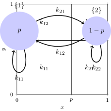
(a) Continuous model: kernel $k_{\mathrm{c}}$ on $\Omega_{\mathrm{c}}=[0,1)$ with the Lebesgue measure.

(b) Discrete model: kernel $k_{\mathrm{d}}$ on $\Omega_{\mathrm{d}}=\{1,2\}$ with the measure $p\delta_{1}+(1-p)\delta_{2}$.

Figure 4. Coupled continuous model (left) and discrete model (right).

7.4.2. Measure preserving function

This section is motivated by the theory of graphons, which are indistinguishable by measure preserving transformation, see [34, Sections 7.3 and 10.7]. Let $(\Omega,\mathscr{F},\mu)$ be a measurable space. We say a measurable function $\varphi$ from $(\Omega,\mathscr{F})$ to itself is measure preserving if $\mu=\varphi_{\#}\mu$. For example the function $\varphi:x\mapsto 2x\mod(1)$ defined on the probability space $([0,1],\mathscr{B}([0,1],\mathrm{Leb})$ is measure preserving.

Let $\varphi$ be measure preserving function on $\Omega$. Let $k_{1}$ be a kernel and $\gamma_{1}$ a function on $\Omega$ such that the model $\mathrm{Param}_{1}=[(\Omega,\mathscr{F},\mu),k_{1},\gamma_{1}]$ satisfies Assumption 2. Let $X_{1}$ be a random variable with probability distribution $\mu$ and let $X_{2}=\varphi(X_{1})$, so that $(X_{1},X_{2})$ is a coupling of $(\Omega,\mathscr{F},\mu)$ with itself. Then for the kernel $k_{2}$ and the function $\gamma_{2}$ defined by:

$$k_{2}(x,y)=k_{1}(\varphi(x),\varphi(y))\quad\text{and}\quad\gamma_{2}(x)=\gamma_{1}(\varphi(x)),$$

the models $\mathrm{Param}_{1}$ and $\mathrm{Param}_{2}=[(\Omega,\mathscr{F},\mu),k_{2},\gamma_{2}]$ are coupled. Roughly speaking, we can give different labels to the features of the population without altering the Pareto and anti-Pareto frontiers.

7.4.3. Model reduction using deterministic coupling

This example is in the spirit of Section 7.4.1, where one merges individual with identical behavior. We consider a SIS model $\mathrm{Param}_{1}=[(\Omega_{1},\mathscr{F}_{1},\mu_{1}),k_{1},\gamma_{1}]$. Let $\varphi$ be a measurable function from $(\Omega_{1},\mathscr{F}_{1})$ to $(\Omega_{2},\mathscr{F}_{2})$. Assume that:

$$\sigma(\gamma_{1})\subset\sigma(\varphi)\quad\text{and}\quad\sigma(k_{1})\subset\sigma(\varphi)\otimes\sigma(\varphi).$$

We can then build an elementary coupling. Let $X_{1}$ and $Y_{1}$ be independent $\mu_{1}$ distributed random elements of $\Omega_{1}$, and set $(X_{2},Y_{2})=(\varphi(X_{1}),\varphi(Y_{1}))$. Since $\sigma(\gamma_{1})\subset\sigma(\varphi)$ and $\sigma(k_{1})\subset\sigma(\varphi)\otimes\sigma(\varphi)$, we get that $\gamma_{1}(X_{1})$ is $\sigma(X_{2})$-measurable and $k_{1}(X_{1},Y_{1})$ is $\sigma(X_{2},Y_{2})$-measurable. According to (50), there exists two measurable functions $\gamma_{2}:\Omega_{2}\to\mathbb{R}$ and $k_{2}:\Omega_{2}\times\Omega_{2}\to\mathbb{R}$ such that $\gamma_{1}=\gamma_{2}\circ\varphi$ and $k_{1}=k_{2}(\varphi\otimes\varphi)$ that is almost surely:

$$\gamma_{1}(X_{1})=\gamma_{2}(X_{2})\quad\text{and}\quad k_{1}(X_{1},Y_{1})=k_{2}(X_{2},Y_{2}).$$

Let $\mu_{2}=\varphi_{\#}\mu_{1}$ be the push-forward measure of $\mu_{1}$ by $\varphi$. Using (49) it is easy to check that the integrability condition from Assumption 2 is fulfilled, so we can consider the reduced model $\mathrm{Param}_{2}=[(\Omega_{2},\mathscr{F}_{2},\mu_{2}),k_{2},\gamma_{2}]$. By Definition 7.1, $\mathrm{Param}_{1}$ is coupled with $\mathrm{Param}_{2}$ through the (deterministic) coupling $\pi$ given by the distribution of $(X_{1},\varphi(X_{1}))$.

Eventually, we get from Corollary 7.4 with $\mathscr{G}=\sigma(\varphi)$, that $\eta_{1}\in\Delta_{1}$ is Pareto optimal if and only if $\mathbb{E}_{1}[\eta_{1}|\,\varphi]$ is Pareto optimal (for the model $\mathrm{Param}_{1}$), where $\mathbb{E}_{1}$ correspond to the expectation with respect to the probability measure $\mu_{1}$ on $(\Omega_{1},\mathscr{F}_{1})$.

8. Technical proofs

8.1. The SIS model: properties of $\mathfrak{I}$ and of the maximal equilibrium

We prove here Theorem 4.6 and Proposition 4.7, and properties of the maximal equilibrium. For the convenience of the reader, we only use references to the results recalled in [7] for positive operators on Banach spaces. For an operator $A$, we denote by $A^{\top}$ its adjoint. We first give a preliminary lemma.

Lemma 8.1.

Suppose Assumption 2 holds, and consider the positive bounded linear integral operator $\mathcal{T}_{k/\gamma}$ on $\mathscr{L}^{\infty}$. If there exists $g\in\mathscr{L}^{\infty}_{+}$, with $\int_{\Omega}g\,\mathrm{d}\mu>0$ and $\lambda>0$ satisfying:

$$\mathcal{T}_{k/\gamma}(g)(x)>\lambda g(x),\quad\text{for all}\quad x\text{ such that }g(x)>0,$$

then we have $\rho(\mathcal{T}_{k/\gamma})>\lambda$.

Proof.

Set $\mathcal{T}=\mathcal{T}_{k/\gamma}$. Let $A=\set{g>0}$ be the support of the function $g$. Let $\mathcal{T}^{\prime}$ be the bounded operator defined by $\mathcal{T}^{\prime}(f)=\mathds{1}_{A}\mathcal{T}(\mathds{1}_{A}f)$. Since $\mathcal{T}^{\prime}(g)=\mathds{1}_{A}\mathcal{T}(\mathds{1}_{A}g)=\mathds{1}_{A}\mathcal{T}(g)>\lambda g$, we deduce from the Collatz-Wielandt formula, see [7, Proposition 3.6], that $\rho(\mathcal{T}^{\prime})\geq\lambda>0$. According to [7, Lemma 3.7 (v)], there exists $v\in L^{q}_{+}\setminus\{0\}$, seen as an element of the topological dual of $\mathscr{L}^{\infty}$, a left Perron eigenfunction of $\mathcal{T}^{\prime}$, that is such that $(\mathcal{T}^{\prime})^{\top}(v)=\rho(\mathcal{T}^{\prime})v$. In particular, we have $v=\mathds{1}_{A}\,v$ and thus $\int_{A}v\,\mathrm{d}\mu>0$ and $\int_{\Omega}vg\,\mathrm{d}\mu>0$. We obtain:

$$(\rho(\mathcal{T}^{\prime})-\lambda)\braket{v,g}=\braket{v,\mathcal{T}^{\prime}(g)-\lambda g}>0.$$

This implies that $\rho(\mathcal{T}^{\prime})>\lambda$. Since $\mathcal{T}-\mathcal{T}^{\prime}$ is a positive operator, we deduce from (26) that $\rho(\mathcal{T})\geq\rho(\mathcal{T}^{\prime})>\lambda$. ∎

We now state an interesting result on the characterization of the maximal equilibrium $\mathfrak{g}$. We keep notations from Sections 2.3 and 2.4 and write $R_{e}$ for $R_{e}[k/\gamma]$. Recall that $R_{0}=R_{e}(\mathds{1})$ and $F$ defined by (18). Let $DF[h]$ denote the bounded linear operator on $\mathscr{L}^{\infty}$ of the derivative of the map $f\mapsto F(f)$ defined on $\mathscr{L}^{\infty}$ at point $h$:

$$DF[h](g)=(1-h)\mathcal{T}_{k}(g)-(\gamma+\mathcal{T}_{k}(h))g\quad\text{for $h,g\in\mathscr{L}^{\infty}$.}$$

Let $s(A)$ denote the spectral bound of the bounded operator $A$, see (33) in [7].

Proposition 8.2.

Suppose Assumption 2 holds and write $R_{e}$ for $R_{e}[k/\gamma]$. Let $h$ in $\Delta$ be an equilibrium, that is $F(h)=0$. The following properties are equivalent:

1. $h=\mathfrak{g}$,

2. $s(DF[h])\leq 0$,

3. $R_{e}((1-h)^{2})\leq 1$.

4. $R_{e}(1-h)\leq 1$.

We also have: $\mathfrak{g}=0\Longleftrightarrow R_{0}\leq 1$; as well as: $\mathfrak{g}\neq 0\Longrightarrow R_{e}(1-\mathfrak{g})=1$.

Proof.

Let $h\in\Delta$ be an equilibrium, that is $F(h)=0$.

Let us show the equivalence between (ii) and (iii). According to [7, Proposition 4.2], $s(DF[h])\leq 0$ if and only if:

$$\rho\left(\mathcal{T}_{\mathrm{k}}\right)\leq 1\quad\text{with}\quad\mathrm{k}(x,y)=(1-h(x))\frac{k(x,y)}{\gamma(y)+\mathcal{T}_{k}(h)(y)}\cdot$$

Since $F(h)=0$, we have $(1-h)/\gamma=1/(\gamma+\mathcal{T}_{k}(h))$. This gives:

(52) $$\mathsf{k}(x,y)=(1-h(x))\frac{k(x,y)(1-h(y))}{\gamma(y)}$$

and thus $\mathcal{T}_{\mathrm{k}}=M_{1-h}\,\mathcal{T}_{k/\gamma}\,M_{1-h}$, where $M_{f}$ is the multiplication operator by $f$. Recall the definition (14) of $R_{e}$. According to (29), we have:

(53) $$\rho\left(\mathcal{T}_{\mathrm{k}}\right)=\rho\left(\mathcal{T}_{k/\gamma}M_{(1-h)^{2}}\right)=R_{e}((1-h)^{2}).$$

This gives the equivalence between (ii) and (iii).

We prove that (i) implies (iv). Suppose that $R_{e}(1-h)>1$. Thanks to (29), we have $\rho(M_{1-h}\mathcal{T}_{k/\gamma})=\rho(\mathcal{T}_{k/\gamma}M_{1-h})=R_{e}(1-h)>1$. According to [7, Lemma 3.7 (v)], there exists $v\in L^{q}_{+}\setminus\{0\}$ a left Perron eigenfunction of $\mathcal{T}_{(1-h)k/\gamma}$, that is $\mathcal{T}_{(1-h)k/\gamma}^{\top}(v)=R_{e}(1-h)v$. Using $F(h)=0$, and thus $(1-h)\mathcal{T}_{k}(h)=\gamma h$, for the last equality, we have:

$$R_{e}(1-h)\braket{v,\gamma h}=\braket{v,(1-h)\mathcal{T}_{k/\gamma}(\gamma h)}=\braket{v,\gamma h}.$$

We get $\braket{v,\gamma h}=0$ and thus $\braket{v,\mathds{1}_{A}}=0$, where $A=\set{h>0}$ denote the support of the function $h$. Since $\mathcal{T}_{(1-h)k/\gamma}^{\top}(v)=R_{e}(1-h)v$ and setting $v^{\prime}=(1-h)v$ (so that $v^{\prime}=v$ $\mu$-almost surely on $A^{c}$), we deduce that:

$$\mathcal{T}_{k^{\prime}/\gamma}^{\top}(v^{\prime})=R_{e}(1-h)v^{\prime},$$

where $k^{\prime}=\mathds{1}_{A^{c}}\,k\,\mathds{1}_{A^{c}}$. This implies that $\rho(\mathcal{T}_{k^{\prime}/\gamma})\geq R_{e}(1-h)$. Since $k^{\prime}=(1-h)k^{\prime}$ and $\mathcal{T}_{k/\gamma}-\mathcal{T}_{k^{\prime}/\gamma}$ is a positive operator as $k-k^{\prime}\geq 0$, we get, using (26) for the inequality, that $\rho(\mathcal{T}_{k^{\prime}/\gamma})=\rho(M_{1-h}\mathcal{T}_{k^{\prime}/\gamma})\leq\rho(M_{1-h}\mathcal{T}_{k/\gamma})=R_{e}(1-h)$. Thus, the spectral radius of $\mathcal{T}_{k^{\prime}/\gamma}$ is equal to $R_{e}(1-h)$. According to [7, Proposition 4.2], since $\rho(\mathcal{T}_{k^{\prime}/\gamma})>1$, there exists $w\in\mathscr{L}^{\infty}_{+}\setminus\{0\}$ and $\lambda>0$ such that:

$$\mathcal{T}_{k^{\prime}}(w)-\gamma w=\lambda w.$$

This also implies that $w=0$ on $A=\set{h>0}$, that is $wh=0$ and thus $w\mathcal{T}_{k}(h)=0$ as $\mathcal{T}_{k}(h)=\gamma h/(1-h)$. Using that $F(h)=0$, $\mathcal{T}_{k}(w)=\mathcal{T}_{k^{\prime}}(w)=(\gamma+\lambda)w$ and $h\mathcal{T}_{k}(w)=0$, we obtain:

$$F(h+w)=w(\lambda-\mathcal{T}_{k}(w)).$$

Taking $\varepsilon>0$ small enough so that $\varepsilon\mathcal{T}_{k}(w)\leq\lambda/2$ and $\varepsilon w\leq 1$, we get $h+\varepsilon w\in\Delta$ and $F(h+\varepsilon w)\geq 0$. Then use Lemma 4.4 to deduce that $h+\varepsilon w\leq\mathfrak{g}$ and thus $h\neq\mathfrak{g}$.

To see that (iv) implies (iii), notice that $(1-h)^{2}\leq(1-h)$, and then deduce from Proposition 4.1 (iii) that $R_{e}((1-h)^{2})\leq R_{e}(1-h)$.

We prove that (iii) implies (i). Notice that $F(g)=0$ and $g\in\Delta$ implies that $g<1$. Assume that $h\neq\mathfrak{g}$. Notice that $\gamma/(1-h)=\gamma+\mathcal{T}_{k}(h)$, so that $\gamma(\mathfrak{g}-h)/(1-h)\in\mathscr{L}^{\infty}_{+}$. An elementary computation, using $F(h)=F(\mathfrak{g})=0$ and $\mathrm{k}$ defined in (52), gives:

$$\mathcal{T}_{\mathrm{k}}\left(\gamma\frac{\mathfrak{g}-h}{1-h}\right)=(1-h)\mathcal{T}_{k}\left(\mathfrak{g}-h\right)=\gamma\frac{\mathfrak{g}-h}{1-\mathfrak{g}}=\frac{1-h}{1-\mathfrak{g}}\,\gamma\frac{\mathfrak{g}-h}{1-h}\cdot$$

Since $h\neq\mathfrak{g}$ and $h\leq\mathfrak{g}$, we deduce that $(1-h)/(1-\mathfrak{g})\geq 1$, with strict inequality on $\set{\mathfrak{g}-h>0}$ which is a set of positive measure. We deduce from Lemma 8.1 (with $k$ replaced by $\mathrm{k}\gamma$) that $\rho\left(\mathcal{T}_{\mathsf{k}}\right)>1$. Then use (53) to conclude.

To conclude notice that $\mathfrak{g}=0\Longleftrightarrow R_{0}\leq 1$ is a consequence of the equivalence between (i) and (iv) with $h=0$ and $R_{0}=R_{e}(\mathds{1})$.

Using that $F(\mathfrak{g})=0$, we get $\mathcal{T}_{k}(\mathfrak{g})=\gamma\mathfrak{g}/(1-\mathfrak{g})$. We deduce that $\mathcal{T}_{k(1-\mathfrak{g})/\gamma}(\mathcal{T}_{k}(\mathfrak{g}))=\mathcal{T}_{k}(\mathfrak{g})$. If $\mathfrak{g}\neq 0$, we get $\mathcal{T}_{k}(\mathfrak{g})\neq 0$ (on a set of positive $\mu$-measure). This implies that $R_{e}(1-\mathfrak{g})\geq 1$. Then use (iv) to deduce that $R_{e}(1-\mathfrak{g})=1$ if $\mathfrak{g}\neq 0$. ∎

In the SIS model, in order to stress, if necessary, the dependence of a quantity $H$, such as $F_{\eta}$, $R_{e}$ or $\mathfrak{g}_{\eta}$, in the parameters $k$ and $\gamma$ (which satisfy Assumption 2) of the model, we shall write $H[k,\gamma]$. Recall that if $k$ and $\gamma$ satisfy Assumption 2, then the kernel $k/\gamma$ has a finite double norm on $L^{p}$ for some $p\in(1,+\infty)$. We now consider the continuity property of the maps $\eta\mapsto\mathfrak{g}_{\eta}[k,\gamma]$ and $(k,\gamma,\eta)\mapsto\mathfrak{g}_{\eta}[k,\gamma]$.

Lemma 8.3.

Let $((k_{n},\gamma_{n}),n\in\mathbb{N})$ and $(k,\gamma)$ be kernels and functions satisfying Assumption 2 and $(\eta_{n},\,n\in\mathbb{N})$ be a sequence of elements of $\Delta$ converging weakly to $\eta$.

1. We have $\lim_{n\rightarrow\infty}\mathfrak{g}_{\eta_{n}}[k,\gamma]=\mathfrak{g}_{\eta}[k,\gamma]$ $\mu$-almost surely.

2. Assume furthermore there exists $p^{\prime}\in(1,+\infty)$ such that $\mathrm{k}=\gamma^{-1}k$ and $(\mathrm{k}_{n}=\gamma^{-1}_{n}k_{n},n\in\mathbb{N})$ have finite double norm on $L^{p^{\prime}}$ and that $\lim_{n\rightarrow\infty}\lVert\mathrm{k}_{n}-\mathrm{k}\rVert_{p^{\prime},q^{\prime}}=0$. Then, we have $\lim_{n\rightarrow\infty}\mathfrak{g}_{\eta_{n}}[k_{n},\gamma_{n}]=\mathfrak{g}_{\eta}[k,\gamma]$ $\mu$-almost surely.

Proof.

The proof of (i) and (ii) being rather similar, we only provide the latter and indicate the difference when necessary. To simplify, we write $g_{n}=\mathfrak{g}_{\eta_{n}}[k_{n},\gamma_{n}]$. We set $h_{n}=\eta_{n}g_{n}\in\Delta$ for $n\in\mathbb{N}$. Since $\Delta$ is sequentially weakly compact, up to extracting a subsequence, we can assume that $h_{n}$ converges weakly to a limit $h\in\Delta$. Since $F_{\eta_{n}}[k_{n},\gamma_{n}](g_{n})=0$ for all $n\in\mathbb{N}$, see (22), we have:

(54) $$g_{n}=\frac{\mathcal{T}_{\mathrm{k}_{n}}(\eta_{n}g_{n})}{1+\mathcal{T}_{\mathrm{k}_{n}}(\eta_{n}g_{n})}=\frac{\mathcal{T}_{\mathrm{k}_{n}}(h_{n})}{1+\mathcal{T}_{\mathrm{k}_{n}}(h_{n})}\cdot$$

We set $g=\mathcal{T}_{\mathrm{k}}(h)/(1+\mathcal{T}_{\mathrm{k}}(h))$. Notice that $\mathcal{T}_{\mathrm{k}_{n}}(h_{n})=(\mathcal{T}_{\mathrm{k}_{n}}-\mathcal{T}_{\mathrm{k}})(h_{n})+\mathcal{T}_{\mathrm{k}}(h_{n})$. We have $\lim_{n\rightarrow\infty}\mathcal{T}_{\mathrm{k}}(h_{n})=\mathcal{T}_{\mathrm{k}}(h)$ pointwise. Since $\lVert(\mathcal{T}_{\mathrm{k}_{n}}-\mathcal{T}_{\mathrm{k}})(h_{n})\rVert_{p^{\prime}}\leq\lVert\mathrm{k}_{n}-\mathrm{k}\rVert_{p^{\prime},q^{\prime}}$, up to taking a sub-sequence, we deduce that $\lim_{n\rightarrow\infty}(\mathcal{T}_{\mathrm{k}_{n}}-\mathcal{T}_{\mathrm{k}})(h_{n})=0$ almost surely. (Notice the previous step is not used in the proof of (i) as $\mathrm{k}_{n}=\mathrm{k}$ and $\lim_{n\rightarrow\infty}\mathcal{T}_{k}(h_{n})=\mathcal{T}_{k}(h)$ pointwise.) This implies that $g_{n}$ converges almost surely to $g$. By the dominated convergence theorem, we deduce that $g_{n}$ converges also in $L^{p}$ to $g$. This proves that $h=\eta g$ almost surely. We get $g=\mathcal{T}_{\mathrm{k}}(\eta g)/(1+\mathcal{T}_{\mathrm{k}}(\eta g))$ and thus $F_{\eta}[k,\gamma](g)=0$: $g$ is an equilibrium for $F_{\eta}[k,\gamma]$. We recall from [8, Section 3] the functional equality $R_{e}[k^{\prime}h]=R_{e}[hk^{\prime}]$, where $k^{\prime}$ is a kernel, $h$ a non-negative functions such that the kernels $k^{\prime}h$ and $hk^{\prime}$ have some finite double norm. We deduce from the weak-continuity and the stability of $R_{e}$, see Theorem 4.2 and Proposition 4.3, that:

$$R_{e}[k/\gamma](\eta(1-g))=R_{e}[\mathrm{k}](\eta(1-g)) =\lim_{n\rightarrow\infty}R_{e}[\mathrm{k}_{n}](\eta_{n}(1-g_{n}))$$

$$=\lim_{n\rightarrow\infty}R_{e}[k_{n}/\gamma_{n}](\eta_{n}(1-g_{n}))$$

$$\leq 1.$$

(Only the weak-continuity of $\eta^{\prime}\mapsto R_{e}[k/\gamma](\eta^{\prime})$ is used in the proof of (i) to get $R_{e}[k/\gamma](\eta(1-g))\leq 1$.) We deduce that property (iv) of Proposition 8.2 holds with $k$ replaced by $k\eta$, and thus property (i) therein implies that $g=\mathfrak{g}_{\eta}[k,\gamma]$. ∎

Proofs of Theorem 4.6 and Proposition 4.7.

Under the assumptions of Lemma 8.3, taking the pair $(k_{n},\gamma_{n})$ equal to $(k,\gamma)$ in the case (i) therein, we deduce that $(\eta_{n}\,\mathfrak{g}_{\eta_{n}}[k_{n},\gamma_{n}],n\in\mathbb{N})$ converges weakly to $\eta\,\mathfrak{g}_{\eta}[k,\gamma]$. This implies that:

$$\lim_{n\rightarrow\infty}\mathfrak{I}[k_{n},\gamma_{n}](\eta_{n})=\lim_{n\rightarrow\infty}\int_{\Omega}\eta_{n}\,\mathfrak{g}_{\eta}[k_{n},\gamma_{n}]\,\mathrm{d}\mu=\int_{\Omega}\eta\,\mathfrak{g}_{\eta}[k,\gamma]\,\mathrm{d}\mu=\mathfrak{I}[k,\gamma](\eta).$$

Taking $(k_{n},\gamma_{n})=(k,\gamma)$ provides the continuity of $\mathfrak{I}[k,\gamma]$ and thus Theorem 4.6. Then, arguing as in the end of the proof of Proposition 4.3, we get Proposition 4.7. ∎

8.2. Coupling and Pareto optimality

We prove here Proposition 7.3. We only consider the SIS model $\mathrm{Param}=[(\Omega,\mathscr{F},\mu),k,\gamma]$, as the kernel model can be handled similarly. We suppose throughout this section that Assumption 2 holds.

The random variables we consider, are defined on a probability space, say $(\Omega_{0},\mathscr{F}_{0},\mathbb{P})$. We recall an elementary result on conditional independence. Let $\mathscr{A}$, $\mathscr{B}$ and $\mathscr{H}$ be $\sigma$-fields subsets of $\mathscr{F}_{0}$, such that $\mathscr{H}\subset\mathscr{A}\cap\mathscr{B}$. Then, according to [28, Theorem 8.9], we have that for any integrable real-valued random variable $X$ which is $\mathscr{B}$-measurable:

(55) $$\text{$\mathscr{A}$ and $\mathscr{B}$ are conditionally independent given $\mathscr{H}$}\,\Longrightarrow\,\mathbb{E}\left[X|\,\mathscr{A}\right]=\mathbb{E}\left[X|\,\mathscr{H}\right].$$

We now state two technical lemmas.

Lemma 8.4 (Measurability).

Let $\mathrm{Param}_{1}$ and $\mathrm{Param}_{2}$ be coupled models with independent coupling $(X_{1},X_{2})$ and $(Y_{1},Y_{2})$. Then the random variable $\gamma_{1}(X_{1})$ is $\sigma(X_{1})\cap\sigma(X_{2})$-measurable. For any measurable function $v:\Omega_{1}\times\Omega_{2}\to\mathbb{R}$, such that $k_{1}(X_{1},Y_{1})v(Y_{1},Y_{2})$ is integrable, the random variable $\mathbb{E}\left[k_{1}(X_{1},Y_{1})v(Y_{1},Y_{2})|X_{1}\right]$ is also $\sigma(X_{1})\cap\sigma(X_{2})$-measurable.

Proof.

The $\sigma(X_{1})\cap\sigma(X_{2})$-measurability of $\gamma_{1}(X_{1})$ is an immediate consequence of the almost-sure equality $\gamma_{1}(X_{1})=\gamma_{2}(X_{2})$. Since $\mathbb{E}\left[k(X_{1},Y_{1})v(Y_{1},Y_{2})|X_{1}\right]$ is $\sigma(X_{1})$-measurable, it remains to prove that it is also $\sigma(X_{2})$-measurable. Since $(X_{1},X_{2})$ is independent from $(Y_{1},Y_{2})$, the $\sigma$-fields $\mathscr{A}=\sigma(X_{1},X_{2})$ and $\mathscr{B}=\sigma(X_{1},Y_{1},Y_{2})$ are conditionally independent given $\mathscr{H}=\sigma(X_{1})$. Using (55), we deduce that:

$$\mathbb{E}\left[k_{1}(X_{1},Y_{1})v(Y_{1},Y_{2})|X_{1}\right]=\mathbb{E}\left[k_{1}(X_{1},Y_{1})v(Y_{1},Y_{2})|X_{1},X_{2}\right].$$

Since $k_{1}(X_{1},Y_{1})=k_{2}(X_{2},Y_{2})$ $\mathbb{P}$-almost surely, we get:

$$\mathbb{E}\left[k_{1}(X_{1},Y_{1})v(Y_{1},Y_{2})|X_{1}\right] =\mathbb{E}\left[k_{2}(X_{2},Y_{2})v(Y_{1},Y_{2})|X_{1},X_{2}\right]$$

$$=\mathbb{E}\left[k_{2}(X_{2},Y_{2})v(Y_{1},Y_{2})|X_{2}\right],$$

where the last equality follows from another application of (55) with $\mathscr{A}=\sigma(X_{1},X_{2})$, $\mathscr{B}=\sigma(X_{2},Y_{1},Y_{2})$ which are conditionally independent given $\mathscr{H}=\sigma(X_{2})$. The last expression is $\sigma(X_{2})$ measurable, so the proof is complete. ∎

In the following key lemma, we simply write $H_{i}$ for $H[\mathrm{Param}_{i}]$ for $H$ the loss functions $R_{e}$ and $\mathfrak{I}$, the cost function $C=C_{\mathrm{uni}}$ and the spectrum $\operatorname{Spec}$.

Lemma 8.5.

If $\mathrm{Param}_{1}$ and $\mathrm{Param}_{2}$ are coupled models, and if the functions $\eta_{1}\in\Delta_{1}$ and $\eta_{2}\in\Delta_{2}$ are coupled, then $\operatorname{Spec}_{1}(\eta_{1})\cup\{0\}=\operatorname{Spec}_{2}(\eta_{2})\cup\{0\}$ and for $H$ any one of the mappings $C_{\mathrm{uni}}$, $R_{e}$ or $\mathfrak{I}$:

(56) $$H_{1}(\eta_{1})=H_{2}(\eta_{2}).$$

Proof.

Let $(X_{1},X_{2})$ and $(Y_{1},Y_{2})$ be two independent couplings, and assume that $\eta_{1}$ and $\eta_{2}$ are coupled through the function $\eta$, see Remark 7.2 (i):

(57) $$\mathbb{E}\left[\eta(X_{1},X_{2})|\,X_{i}\right]=\eta_{i}(X_{i})\quad\text{for $i\in\{1,2\}$}.$$

Step 1: The cost function ($H=C_{\mathrm{uni}}$). We directly have:

$$C_{1}(\eta_{1})=1-\mathbb{E}\left[\eta_{1}(X_{1})\right]=1-\mathbb{E}\left[\eta(X_{1},X_{2})\right]=1-\mathbb{E}\left[\eta_{2}(X_{2})\right]=C_{2}(\eta_{2}).$$

Step 2: The spectrum and the effective reproduction function ($H=R_{e}$). Set $\mathrm{k}_{i}=k_{i}/\gamma_{i}$ for $i\in\{1,2\}$. Let $\lambda$ be a non-zero eigenvalue of $T_{\mathrm{k}_{1}\eta_{1}}$ associated with an eigenvector $v_{1}$. Notice that $\mathrm{k}(X_{1},Y_{1})\eta_{1}(Y_{1})v(Y_{1})$ is integrable thanks to the integrability condition from Assumption 2. By definition of eigenvectors, $v_{1}(X_{1})$ is a version of the conditional expectation:

$$\lambda^{-1}\mathbb{E}\left[\mathrm{k}_{1}(X_{1},Y_{1})\,\eta_{1}(Y_{1})v_{1}(Y_{1})|X_{1}\right].$$

By Lemma 8.4 applied to the function $v(y_{1},y_{2})=(v_{1}\eta_{1}/\gamma_{1})(y_{1})$, the real-valued random variable $v_{1}(X_{1})$ is $\sigma(X_{1})\cap\sigma(X_{2})$-measurable and thus $\sigma(X_{2})$-measurable. Thanks to (50), there exists $v_{2}$ such that $v_{2}(X_{2})=v_{1}(X_{1})$ almost surely. Since $(Y_{1},Y_{2})$ is distributed as $(X_{1},X_{2})$, we deduce that (57) holds also with $(X_{1},X_{2})$ replaced by $(Y_{1},Y_{2})$ and that $v_{2}(Y_{2})=v_{1}(Y_{1})$ almost surely. Recall that $\mathrm{k}_{i}=k_{i}/\gamma_{i}$, so that $\mathrm{k}_{1}(X_{1},Y_{1})=\mathrm{k}_{2}(X_{2},Y_{2})$ almost surely. We may now compute:

(58) $$\lambda v_{2}(X_{2}) =\lambda v_{1}(X_{1})$$

$$=\mathbb{E}\left[k_{1}(X_{1},Y_{1})\,\eta_{1}(Y_{1})v_{1}(Y_{1})|X_{1}\right]$$

$$=\mathbb{E}\left[\mathrm{k}_{1}(X_{1},Y_{1})\,\eta(Y_{1},Y_{2})v_{1}(Y_{1})|X_{1}\right] (Y_{1},X_{1})$$ (de-conditioning on )

$$=\mathbb{E}\left[\mathrm{k}_{1}(X_{1},Y_{1})\,\eta(Y_{1},Y_{2})v_{1}(Y_{1})|X_{2}\right]$$ (Lemma 8.4)

$$=\mathbb{E}\left[\mathrm{k}_{2}(X_{2},Y_{2})\,\eta(Y_{1},Y_{2})v_{2}(Y_{2})|X_{2}\right]$$ (a.s. equality)

$$=\mathbb{E}\left[\mathrm{k}_{2}(X_{2},Y_{2})\,\eta_{2}(Y_{2})v_{2}(Y_{2})|X_{2}\right] (Y_{2},X_{2})$$ (conditioning on )

$$=T_{\mathrm{k}_{2}\eta_{2}}v_{2}(X_{2}).$$

Since the distribution of $X_{2}$ is $\mu_{2}$, we have $\lambda v_{2}=T_{\mathrm{k}_{2}\eta_{2}}v_{2}$ $\mu_{2}$-almost surely. Therefore $\lambda$ is also an eigenvalue for $T_{\mathrm{k}_{2}\eta_{2}}$. By symmetry we deduce that the spectrum up to $\{0\}$ of $T_{\mathrm{k}_{1}\eta_{1}}$ and $T_{\mathrm{k}_{2}\eta_{2}}$ coincide, that is $\operatorname{Spec}_{1}(\eta_{1})\cup\{0\}=\operatorname{Spec}_{2}(\eta_{2})\cup\{0\}$, and in particular the spectral radius coincide.

Step 3: The total proportion of infected population function ($H=\mathfrak{I}$). We assume without loss of generality that $\rho(\mathcal{T}_{k_{1}/\gamma_{1}})>1$, which is equivalent to $\rho(\mathcal{T}_{k_{2}/\gamma_{2}})>1$, thanks to (56) with $H=R_{e}$ and $\eta_{1}=\eta_{2}=1$. Let $g_{1}=\mathfrak{g}_{\eta_{1}}$ be the maximal equilibrium for the model $\mathrm{Param}_{1}$. Since $F_{\eta_{1}}(g_{1})=0$, see (22), we have:

(59) $$g_{1}=\frac{\mathcal{T}_{k_{1}}(\eta_{1}g_{1})}{\gamma_{1}+\mathcal{T}_{k_{1}}(\eta_{1}g_{1})}\cdot$$

By Lemma 8.4, this implies that $g_{1}(X_{1})$ is $\sigma(X_{1})\cap\sigma(X_{2})$ measurable. Thus, there exists $g^{\prime}_{2}$ such that $g^{\prime}_{2}(X_{2})=g_{1}(X_{1})$ $\mathbb{P}$-almost surely.. Therefore, by the same computation as in (58):

$$\mathcal{T}_{k_{1}}(\eta_{1}g_{1})(X_{1})=\mathcal{T}_{k_{2}}(\eta_{2}g^{\prime}_{2})(X_{2})\quad\mathbb{P}-\text{a.s.}$$

We set:

(60) $$g_{2}=\frac{\mathcal{T}_{k_{2}}(\eta_{2}g^{\prime}_{2})}{\gamma_{2}+\mathcal{T}_{k_{2}}(\eta_{2}g^{\prime}_{2})}\cdot$$

Then, we deduce from (59) that $g_{2}(X_{2})=g^{\prime}_{2}(X_{2})$ $\mathbb{P}$-almost surely, that is $g_{2}=g^{\prime}_{2}$ $\mu_{2}$-almost surely. Thus (60) holds with $g^{\prime}_{2}$ replaced by $g_{2}$. In other words, $g_{2}$ satisfies (22): it is an equilibrium for the model given by $\mathrm{Param}_{2}$.

Let us now prove that $g_{2}$ is in fact the maximal equilibrium. Since $g_{2}(X_{2})=g_{1}(X_{1})$ $\mathbb{P}$-almost surely and $g_{1}(X_{1})$ is $\sigma(X_{1})\cap\sigma(X_{2})$-measurable, we deduce from Remark 7.2 (ii), that $(1-g_{1})$ and $(1-g_{2})$ are coupled, so $R_{e}[\mathrm{Param}_{1}](1-g_{1})=R_{e}[\mathrm{Param}_{2}](1-g_{2})$, by Property (56) applied to $H=R_{e}$. Since $R_{0}>1$ and $g_{1}$ is the maximal equilibrium for $\mathrm{Param}_{1}$, we deduce from Proposition 8.2 that $R_{e}[\mathrm{Param}_{1}](1-g_{1})=1$. Using again Proposition 8.2, this gives that $g_{2}$ is the maximal equilibrium for $\mathrm{Param}_{2}$.

We may now compute:

$$\mathfrak{I}_{1}(\eta_{1}) =\mathbb{E}\left[\eta_{1}(X_{1})\,g_{1}(X_{1})\right]$$

$$=\mathbb{E}\left[\eta(X_{1},X_{2})\,g_{1}(X_{1})\right] X_{1}$$ (deconditioning on )

$$=\mathbb{E}\left[\eta(X_{1},X_{2})\,g_{2}(X_{2})\right]$$ ( a.s. equality)

$$=\mathbb{E}\left[\eta_{2}(X_{2})\,g_{2}(X_{2})\right] X_{2}$$ (conditioning on )

$$=\mathfrak{I}_{2}(\eta_{2}),$$

thus (56) holds for $H=\mathfrak{I}$, and the proof is complete. ∎

We now give the proof of Proposition 7.3. Its first part is an elementary consequence of the Lemma 8.5; and the second part is a direct consequence of Remark 7.2 (iii).

References

• [1] Philip M. Anselone “Collectively compact operator approximation theory and applications to integral equations” Prentice-Hall, 1971
• [2] Philip M. Anselone and John W. Lee “Spectral properties of integral operators with nonnegative kernels” In Linear Algebra and its Applications 9 Elsevier BV, 1974, pp. 67–87 DOI: 10.1016/0024-3795(74)90027-5
• [3] Béla Bollobás, Svante Janson and Oliver Riordan “The phase transition in inhomogeneous random graphs” In Random Structures Algorithms 31.1, 2007, pp. 3–122
• [4] Tom Britton, Frank Ball and Pieter Trapman “A mathematical model reveals the influence of population heterogeneity on herd immunity to SARS-CoV-2” In Science 369.6505 American Association for the Advancement of Science (AAAS), 2020, pp. 846–849 DOI: 10.1126/science.abc6810
• [5] Laura Burlando “Continuity of spectrum and spectral radius in Banach algebras” In Banach Center Publications 30, 1994, pp. 53–100
• [6] John B. Conway “A course in functional analysis” 96, Graduate Texts in Mathematics Springer-Verlag, 1990
• [7] Jean-François Delmas, Dylan Dronnier and Pierre-André Zitt “An Infinite-Dimensional SIS Model”, 2020 arXiv:2006.08241 [math.DS]
• [8] Jean-François Delmas, Dylan Dronnier and Pierre-André Zitt “Effective reproduction number: convexity, invariance and cordons sanitaires”, 2021
• [9] Jean-François Delmas, Dylan Dronnier and Pierre-André Zitt “Optimal vaccination for a 2 sub-populations SIS model”, 2021
• [10] Jean-François Delmas, Dylan Dronnier and Pierre-André Zitt “Optimal vaccination: various (counter) intuitive examples”, 2021
• [11] Jean-François Delmas, Dylan Dronnier and Pierre-André Zitt “Vaccinating higly connected people is (sometimes) optimal”, 2021
• [12] O. Diekmann, J… Heesterbeek and J… Metz “On the definition and the computation of the basic reproduction ratio ${R}_{0}$ in models for infectious diseases in heterogeneous populations” In Journal of Mathematical Biology 28.4, 1990, pp. 365–382 DOI: 10.1007/BF00178324
• [13] Klaus Dietz “Transmission and control of arbovirus diseases” In Epidemiology 104 SIAM Philadelphia, 1975, pp. 104–121
• [14] Evelot Duijzer, Willem Jaarsveld, Jacco Wallinga and Rommert Dekker “The most efficient critical vaccination coverage and its equivalence with maximizing the herd effect” In Mathematical Biosciences 282 Elsevier BV, 2016, pp. 68–81 DOI: 10.1016/j.mbs.2016.09.017
• [15] Lotty E. Duijzer, Willem L. Jaarsveld, Jacco Wallinga and Rommert Dekker “Dose-optimal vaccine allocation over multiple populations” In Production and Operations Management 27.1 Wiley, 2018, pp. 143–159 DOI: 10.1111/poms.12788
• [16] Friedrich Esser and Frank Harary “On the spectrum of a complete multipartite graph” In European Journal of Combinatorics 1.3, 1980, pp. 211–218 DOI: 10.1016/S0195-6698(80)80004-7
• [17] Zhilan Feng, Andrew N. Hill, Aaron T. Curns and John W. Glasser “Evaluating targeted interventions via meta-population models with multi-level mixing” In Mathematical Biosciences 287, 2017, pp. 93–104 DOI: 10.1016/j.mbs.2016.09.013
• [18] Zhilan Feng, Andrew N. Hill, Philip J. Smith and John W. Glasser “An elaboration of theory about preventing outbreaks in homogeneous populations to include heterogeneity or preferential mixing” In Journal of Theoretical Biology 386, 2015, pp. 177–187 DOI: 10.1016/j.jtbi.2015.09.006
• [19] Paul Fine, Ken Eames and David L. Heymann “Herd Immunity: A Rough Guide” In Clinical Infectious Diseases 52.7, 2011, pp. 911–916 DOI: 10.1093/cid/cir007
• [20] A. Ganesh, L. Massoulie and D. Towsley “The effect of network topology on the spread of epidemics” In Proceedings IEEE 24th Annual Joint Conference of the IEEE Computer and Communications Societies. IEEE, 2005 DOI: 10.1109/infcom.2005.1498374
• [21] E. Goldstein, A. Apolloni, B. Lewis, J.. Miller, M. Macauley, S. Eubank, M. Lipsitch and J. Wallinga “Distribution of vaccine/antivirals and the ‘least spread line’ in a stratified population” In Journal of The Royal Society Interface 7.46 The Royal Society, 2010, pp. 755–764 DOI: 10.1098/rsif.2009.0393
• [22] J.. Grobler “Compactness conditions for integral operators in Banach function spaces” In Indagationes Mathmaticae (Proceedings) 32, 1970, pp. 287–294
• [23] Charles J.. Halberg and Angus E. Taylor “On the spectra of linked operators” In Pacific Journal of Mathematics 6, 1956, pp. 283–290
• [24] Herbert W. Hethcote and James A. Yorke “Gonorrhea Transmission Dynamics and Control” 56, Lecture Notes in Biomathematics Springer-Verlag, 1984 DOI: 10.1007/978-3-662-07544-9
• [25] Andrew N. Hill and Ira M. Longini Jr. “The critical vaccination fraction for heterogeneous epidemic models” In Mathematical Biosciences 181.1, 2003, pp. 85–106
• [26] Stephen Huggett and David Jordan “A topological aperitif” Springer-Verlag, 2009
• [27] Svante Janson “Graphons, cut norm and distance, couplings and rearrangements”, NYJM Monographs New York Journal of Mathematics, 2013
• [28] Olav Kallenberg “Foundations of modern probability” 99, Probability Theory and Stochastic Modelling Springer-Verlag, 2021, pp. 946 DOI: 10.1007/978-3-030-61871-1
• [29] Tosio Kato “Perturbation theory for linear operators” Springer-Verlag, 2013
• [30] Matthew James Keeling and Pejman Rohani “Modeling infectious diseases in humans and animals” Princeton University Press, 2008
• [31] Benoît R. Kloeckner “Effective perturbation theory for simple isolated eigenvalues of linear operators” In Journal of Operator Theory 81.1, 2019, pp. 175–194
• [32] Hermann König “Eigenvalue distribution of compact operators” 16, Operator Theory: Advances and Applications Birkhäuser Verlag, 1986
• [33] Ana Lajmanovich and James A. Yorke “A deterministic model for gonorrhea in a nonhomogeneous population” In Mathematical Biosciences 28.3, 1976, pp. 221–236 DOI: 10.1016/0025-5564(76)90125-5
• [34] László Lovász “Large networks and graph limits”, American Mathematical Society colloquium publications 60 American Mathematical Society, 2012
• [35] Ivo Marek “Frobenius theory of positive operators: comparison theorems and applications” In SIAM Journal on Applied Mathematics 19.3 Society for IndustrialApplied Mathematics, 1970, pp. 607–628
• [36] Kaisa Miettinen “Nonlinear multiobjective optimization” In International Series in Operations Research & Management Science Springer-Verlag, 1998 DOI: 10.1007/978-1-4615-5563-6
• [37] J.. Newburgh “The variation of spectra” In Duke Mathematical Journal 18.1 Duke University Press, 1951, pp. 165–176 DOI: 10.1215/S0012-7094-51-01813-3
• [38] Gayane Poghotanyan, Zhilan Feng, John W. Glasser and Andrew N. Hill “Constrained minimization problems for the reproduction number in meta-population models” In Journal of Mathematical Biology 77.6, 2018, pp. 1795–1831 DOI: 10.1007/s00285-018-1216-z
• [39] Juan G. Restrepo, Edward Ott and Brian R. Hunt “Characterizing the Dynamical Importance of Network Nodes and Links” In Physical Review Letters 97.9 American Physical Society, 2006 DOI: 10.1103/physrevlett.97.094102
• [40] Sudip Saha, Abhijin Adiga, B. Prakash and Anil Kumar S. Vullikanti “Approximation Algorithms for Reducing the Spectral Radius to Control Epidemic Spread” In Proceedings of the 2015 SIAM International Conference on Data Mining Society for IndustrialApplied Mathematics, 2015 DOI: 10.1137/1.9781611974010.64
• [41] H.. Schaefer “Banach lattices and positive operators” 215, Grundlehren der mathematischen Wissenschaften Springer-Verlag, 1974
• [42] C E Gordon Smith “Prospects for the control of infectious disease” In Proceedings of the Royal Society of Medicine 63.11 Pt 2, 1970, pp. 1181–1190
• [43] Peter G. Smith “Concepts of herd protection and immunity” In Procedia in Vaccinology 2.2, 2010, pp. 134–139 DOI: 10.1016/j.provac.2010.07.005
• [44] Margaret Somerville, K. Kumaran and Rob Anderson “Public health and epidemiology at a glance” John Wiley & Sons, 2016
• [45] Dragan Stevanović, Ivan Gutman and Masood U. Rehman “On spectral radius and energy of complete multipartite graphs” In Ars Mathematica Contemporanea 9.1, 2015, pp. 109–113 DOI: 10.26493/1855-3974.499.103
• [46] Piet Van Mieghem, Dragan Stevanović, Fernando Kuipers, Cong Li, Ruud Bovenkamp, Daijie Liu and Huijuan Wang “Decreasing the spectral radius of a graph by link removals” In Physical Review E 84.1 American Physical Society (APS), 2011 DOI: 10.1103/physreve.84.016101
• [47] Henry Zhao and Zhilan Feng “Identifying optimal vaccination strategies via economic and epidemiological modeling” In Journal of Biological Systems 27.4 World Scientific Pub Co Pte Lt, 2019, pp. 423–446 DOI: 10.1142/s0218339019400011