Statistical Characterization of Random Errors Present in Synchrophasor Measurements

Abstract

The statistical characterization of the measurement errors of a phasor measurement unit (PMU) is currently receiving considerable interest in the power systems community. This paper focuses on the characteristics of the errors in magnitude and angle measurements introduced only by the PMU device (called random errors in this paper), during ambient conditions, using a high-precision calibrator. The experimental results indicate that the random errors follow a non-Gaussian distribution. They also show that the M-class and P-class PMUs have distinct error characteristics. The results of this analysis will help researchers design algorithms that account for the non-Gaussian nature of the errors in synchrophasor measurements, thereby improving the practical utility of the said-algorithms in addition to building on precedence for using high-precision calibrators to perform accurate error tests.

I Introduction

Phasor measurement units (PMUs) measure magnitude, phase angle, frequency, and rate-of-change-of-frequency (ROCOF) of electrical signals and play a critical role in real-time monitoring, protection, and control of modern power systems. The measurements obtained from PMUs are affected not only by the PMU device mechanics, but also by other components in the measurement chain, such as instrument transformers and cables. As such, PMU errors can be of two types: systematic and random [1]. Systematic errors occur due to the erratic behavior of the components present in the measurement chain (such as current transformer saturation), while random errors occur due to the PMU device itself (e.g., components internal to the PMU, response of the PMU to normal changes occurring in the system). The focus of this paper is on the random errors of a PMU.

PMUs are being adopted rapidly by utilities and more power system applications are making use of them to achieve better performance [2, 3]. Knowledge of the nature of the errors in PMU measurements is extremely important because by understanding their statistical characteristics, researchers can design better algorithms that have more practical utility. The scope of this research is limited to characterizing the random errors that occur during ambient conditions (i.e., in absence of faults, oscillations, time-synchronization issues, or device saturation), since a power system stays in this condition most of the time.

Traditionally, PMU measurement noise was always assumed to follow a Gaussian distribution. However, there has been some recent interest in understanding the exact statistical nature of PMU measurement noises. Brown et al. tried to quantify the PMU measurement noises using field PMU data [4]. They conditioned the data, segregated the steady state data, and used filtering techniques to extract the errors. Studying the nature of these errors they concluded that it has a zero mean Gaussian distribution. Later, Wang et al., using redundant field PMU measurements and employing the fact that the difference of two random variables following a Gaussian distribution is a necessary condition for the individual random variables to be Gaussian, showed that PMU measurement errors do not necessarily follow a Gaussian distribution [5]. Ahmad et al. further verified this argument using data driven filtering techniques [1]. In particular, they used an adaptive moving window median absolute deviation method to extract the errors from both synthetic data as well as field data. They concluded from their analysis that the error followed a 3-component Gaussian mixture model (GMM) distribution, primarily due to device saturation.

In this paper, we have used a high precision Fluke calibrator (Fluke 6135A) [6] to characterize the random errors found in PMU measurements. Although very expensive, a high precision calibrator is the best way to extract PMU measurement errors. This is because it precludes the assumption of presence of a calibrated PMU at every substation, which is employed in many state-of-the-art error extraction techniques [1, 5].

The focus of this paper is on discovering error distributions during ambient system conditions. Therefore, the slowly changing dynamics of the power system as specified in the IEEE C37.118.1-2011 Standard [7] were applied to the device-under-test (DUT). The analysis was carried out for a P-class PMU as well as an M-class PMU using normality tests as well as more quantitative metrics (higher-order moments). The results indicate that even under ambient conditions, the random errors in P-class and M-class PMUs have a distinct non-Gaussian error distribution.

The rest of the paper is structured as follows. Section II describes the mathematical basis for this work. Sections III and IV explain the test setup and results, respectively. The conclusion and future scope are identified in Section V.

II Mathematical Background

II-A Dynamic Tests

In this research, three dynamic tests described in the IEEE C37.118.1-2011 Standard [7], namely, the amplitude modulation (AM) test, the phase modulation (PM) test, and the frequency ramp (FR) test, have been carried out, and the statistical analysis of the extracted errors have been reported.

The signal for the AM and PM tests for the $a$-phase can be mathematically represented as:

$$X_{a}=X_{m}[1+k_{x}cos(\omega t)]cos[w_{0}t+k_{a}cos(wt-\pi)]$$ (1)

where, $k_{x}$ and $k_{a}$ represent the amplitude and phase modulation factors, respectively. For the $b$ and $c$ phases, the equation would be similar except for the fact that the phase would be lagging and leading by $\frac{2\pi}{3}$, respectively. The positive sequence signal can be obtained from the $abc$ phases. If $T$ is the phasor reporting interval and $n$ is any integer then the phasor representation of the positive sequence measurement obtained at $t=nT$ is given by:

$$X(nT)=\{\frac{X_{m}}{\sqrt{2}}\}[1+k_{x}cos(\omega nT)]\angle\{k_{a}cos(\omega nT-\pi)\}$$ (2)

The electrical signals generated in accordance with (2), i.e. the true values, are passed to the DUT. The values obtained at the output of the DUT are saved as the measured values. The relative magnitude error (RME) is calculated as:

$$RME =\frac{X_{m_{true}}-X_{m_{meas}}}{X_{m_{true}}}$$ (3)

The phase angle error is given by:

$$PE =X_{ang_{true}}-X_{ang_{meas}}$$ (4)

For the FR tests, the positive sequence signal is written as:

$$X_{1}=X_{m}cos(w_{0}t+\pi R_{f}t^{2})$$ (5)

where, $R_{f}=\frac{df}{dt}$. At reporting time tags, $t=nT$, the phasor measurements can be expressed as:

$$X(nT)=\frac{X_{m}}{\sqrt{2}}\angle\{\pi R_{f}(nT)^{2}\}$$ (6)

The relative magnitude error and phase angle error corresponding to these tests are calculated for both P-class and M-class PMUs. Note that the relative magnitude error is the ratio of the magnitude error and the true value (reported as a percentage value), while the phase angle error is the difference between the measured value and the true value (reported in degrees). Finally, the histograms of these errors are plotted to draw inferences regarding the distribution of the random errors, while numerical and statistical tests are performed to quantify the parameters of the distribution.

II-B Normality Tests

Normality tests are primarily used to verify if a data set can be reasonably modeled by a Gaussian distribution or not. Two normality tests that are used in this study are the Shapiro-Wilks test and the Kolmogorov-Smirnov test.

The Shapiro-Wilks test operates by testing the data set across a hypothesis of normality, creating a $p$-value that, within a certain $alpha$ significance level, indicates whether the researchers can accept or reject the null hypothesis that the data fits the normal distribution. The critical value of $alpha$ is a cut-off point where the experiment may reject a null hypothesis in error. Common values of $alpha$ used in practice are 0.1, 0.05, and 0.01, respectively [8]. For this experiment, the value of $alpha$ was set at 0.05, indicating that the probability of a Type 1 error (falsely rejecting a null hypothesis that is actually true) is less than 5%.

The Kolmogorov-Smirnov test is based on the empirical cumulative distribution function (ECDF). The null hypothesis in this case is that both sets of input data are coming from the same distribution [9]. Thus, the Kolmogorov-Smirnov test calculates the distance between ECDFs of the given error distribution and corresponding Gaussian distribution to determine the similarity between the two. The next section describes the test setup created for this study.

III Hardware Test Setup

In order to provide accurate time-synchronized instrument transformer-level signals to the DUT, a Fluke 6135A PMU calibration unit was employed. This hardware device generates time-synchronized electrical waveforms of voltage and current that are guaranteed to meet 0.007% accuracy for the tests specified in [6]. Each DUT was connected to the Fluke 6135A such that its voltage and current input terminals were wired to the voltage and current output terminals of the Fluke 6135A. Fig. 1 depicts one of the DUTs (an M-class PMU) connected to the Fluke 6135A.

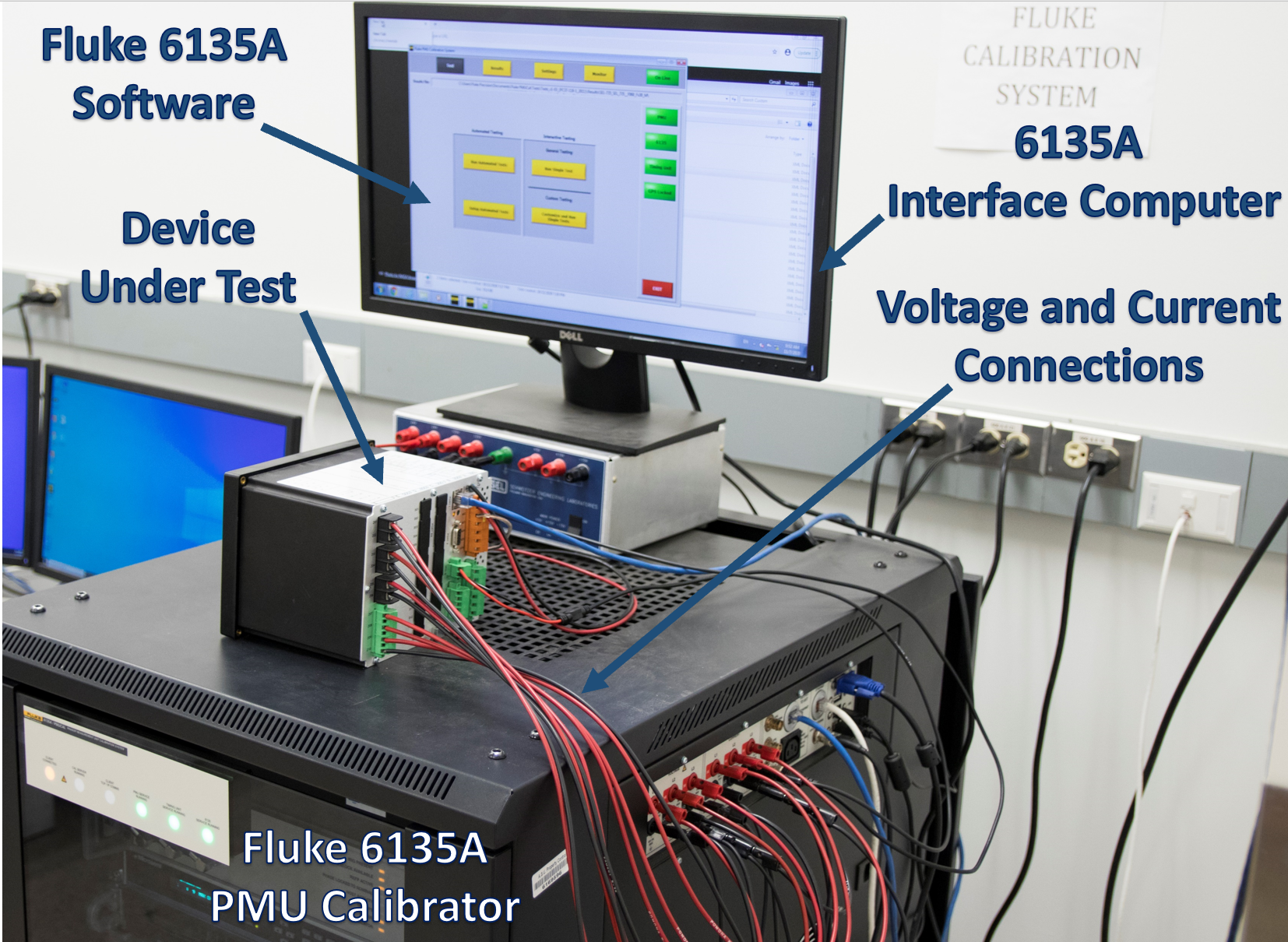
Figure 1: Hardware Test Setup

The Fluke 6135A PMU calibrator can be configured to perform all the steady-state and dynamic performance tests required by the IEEE C37.118-2011 [7]. When each test is performed by the calibrator, a spreadsheet of synchrophasor measurements and their respective nominal values (as produced by the calibrator at its output terminals) are reported by the software suite provided with the calibrator. These test report spreadsheets also include the errors in angle and magnitude between the measured and the nominal synchrophasor, and it is these error values that were extracted from each test to characterize the errors in the DUT.

The goal of this characterization experiment is to determine the behavior of the PMUs under dynamic conditions that are reflective of the behavior of an actual power system during ambient conditions. The IEEE C37.118.1a-2014 Standard [10] specifies the parameters for the dynamic tests for sinusoidal AM, sinusoidal PM, and linear frequency ramping. In the case of the AM and PM tests, the minimum modulation frequency was employed. For the FR tests, a gradually rising frequency ramp test and a gradually falling frequency ramp test were selected. In each case, the test parameters were selected as specified in the IEEE C37.118.1a-2014 Standard [10]; the numerical values of the parameters are given in Section IV-B. In order to extract sufficient data to plot histograms of the error distributions of interest for each test, the relevant tests were performed repeatedly until a total of 18,000 samples (10 minutes worth of test data at 30 samples per second) were collected. These error values were concatenated together, plotted, and checked for consistency. The latter was ensured by repeating every test three times. Afterwards, the most relevant trends and characteristics of the errors were noted and conclusions were drawn on their basis.

IV Results

IV-A Observations

Some general observations made from the experiments are summarized below:

• For the P-class PMU, when running the PM tests, the phase angle errors were found to be continuous, while the relative magnitude errors were found to be discrete (here, discrete means that the error values were placed into distinct bins rather than being continuously spread).

• For the P-class PMU, when running the AM tests, the relative magnitude errors were found to be continuous, while the phase angle errors were discrete.

• For both the P-class as well as the M-class PMU, the error distributions appeared to have a constant bias (a non zero mean value) for all the tests.

• The Shapiro-Wilks and the Kolmogorov-Smirnov tests substantiated the hypothesis that the random errors in both P-class and M-class PMU measurements have non-Gaussian distributions.

IV-B Error Characteristics for the P-class PMU

The error characterization studies were conducted for each of the three phases as well as the positive sequence. For sake of brevity, only the results of positive sequence tests corresponding to ambient power system operating conditions (slowly changing system dynamics) are discussed here. The following histograms correspond to the 0.1 Hz PM, 0.1 Hz AM, up to +0.03 Hz/sec FR up, and up to -0.03 Hz/sec FR down, tests [7]. Fig. 2 shows the phase angle error distribution for the PM tests. By repeating the tests three times it was confirmed that the shapes and ranges of the histograms were consistent. Two distinct peaks are visible in this error histogram, indicating that it can be more accurately represented using a two-component GMM as opposed to a Gaussian distribution.

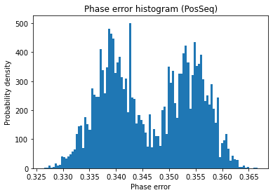
Figure 2: P-class - phase angle error histogram - phase modulation

Fig. 3 shows the relative magnitude error histogram of the same device for AM tests. The normality tests and the skewness & kurtosis parameters (calculated during the quantitative analysis in Section IV-D) reinforce the hypothesis that the relative magnitude error distributions are non-Gaussian for this case as well.

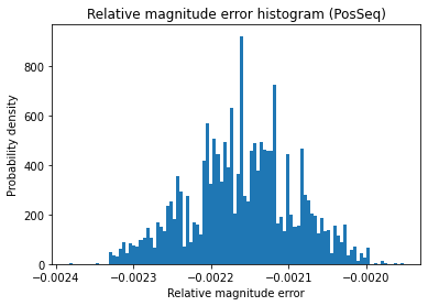
Figure 3: P-class - relative magnitude error histogram - amplitude modulation

Figs. 4 and 5 represent the relative magnitude error histogram and phase angle error histogram for the FR up test. The relative magnitude error histogram shows discrete values with change in frequencies. The phase angle error histogram has error values distributed continuously. The normality tests and the skewness and kurtosis values (see Section IV-D) further validate the non-Gaussian nature of this error distribution.

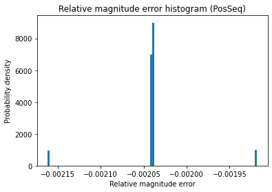
Figure 4: P-class - relative magnitude error histogram - frequency ramp up

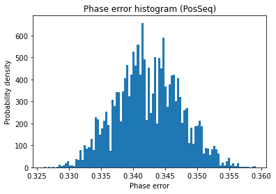
Figure 5: P-class - phase angle error histogram - frequency ramp up

IV-C Error Characteristics for the M-Class PMU

The same set of tests (although with slightly different sets of parameters as mentioned in the IEEE C37.118.1-2011 Standard [7]) when applied to the M-class PMU also resulted in non-Gaussian histograms for the random errors. Fig. 6 represents the phase angle error histogram for the PM test. From the histogram, five distinct peaks can be observed (as opposed to two in the case of the P-class PMU). As expected, the normality tests confirmed that the distribution was non-Gaussian. It was found that this error distribution could be best approximated by using a five-component GMM or a five-component beta mixture model.

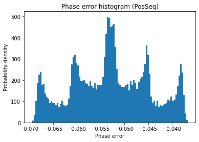
Figure 6: M-class - phase angle error histogram - phase modulation

The relative magnitude error histogram for AM test for the same device is shown in Fig. 7. Even though visual inspection of this histogram reveals that it is indeed a non-Gaussian distribution with two-peaks, since the range is extremely small, this distribution may not have much significance in practice.

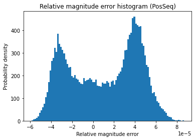
Figure 7: M-class - relative magnitude error histogram - amplitude modulation

The relative magnitude error histogram for FR down test is shown in Fig. 8. It can be observed that this histogram is asymmetric with a heavier tail towards the left side. The phase angle error histogram for the FR down test is shown in Fig. 9. The error histogram can be best modeled using a tri-modal distribution as the individual components are distinct.

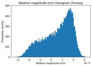
Figure 8: M-class - relative magnitude error histogram - frequency ramp down

Figure 9: M-class - phase angle error histogram - frequency ramp down

IV-D Quantitative analysis

In addition to the normality tests, some statistical quantities which determine the features of a probability distribution were also calculated and used to verify the non-Gaussian nature of the random errors in PMU measurements. The mean, standard deviation, skewness, and kurtosis are the first, second, third, and fourth moments, respectively, and convey specific attributes of a distribution. The mean and standard deviation represent the average value and the range of the distribution. The skewness of the distribution indicates if the error distribution is asymmetric (either right-tailed or left-tailed); i.e., for a Gaussian distribution the skewness value is negligibly small (ideally zero). The kurtosis denotes the amount of data present towards both ends relative to the center of the distribution; this should also be negligible (ideally zero) for a Gaussian distribution.

Tables I and II show the phase angle errors and the relative magnitude errors for the P-class PMU, respectively. PM, AM, and FR represent the three dynamic tests, namely, phase modulation, amplitude modulation and frequency ramp. The relatively large values of skewness and kurtosis in these tables are proof of the non-Gaussian nature of the random errors in PMU measurements during ambient conditions.

TABLE I: Phase Angle Error - P-class PMU

	Mean	Median	Std. dev.	Skewness	Kurtosis
PM	0.361392	0.36019	0.00779	0.077721	-1.426
AM	0.344971	0.34570	0.00918	-0.01066	-1.26174
FR	0.342382	0.342188	0.00504	0.068226	-0.31194

TABLE II: Relative Magnitude Error - P-class PMU

	Mean	Median	Std. dev.	Skewness	Kurtosis
PM	-0.00211	-0.00216	5.97E-05	0.43024	-1.79
AM	0.342005	0.340205	0.00443	0.18960	-0.22678
FR	-0.00201	-0.00204	5.45E-05	1.00192	-0.8246

Tables III and IV denote the phase angle errors and the relative magnitude errors for the M-class PMU, respectively. These tables validate the following observations: (a) the non-Gaussian nature of the error distributions, and (b) the existence of bias in the error values.

TABLE III: Phase Angle Error - M-class PMU

	Mean	Median	Std. dev.	Skewness	Kurtosis
PM	-0.053	-0.053	0.00818	0.00592	-0.747
AM	-0.046	-0.046	0.00591	0.00724	-1.48
FR	-0.04598	-0.045986	0.00589	-0.00910	-1.47634

TABLE IV: Relative Magnitude Error - M-class PMU

	Mean	Median	Std. dev.	Skewness	Kurtosis
PM	1.55E-05	1.55E-05	7.51E-06	0.0178	-0.0101
AM	1.29E-05	1.78E-05	3.32E-05	-0.152	-1.33
FR	1.15E-05	1.73E-05	2.56E-05	-0.56436	-0.68725

IV-E Discussion

For the PM test on the M-Class PMU, the relative magnitude errors were not only minuscule, but also across all relative magnitude errors the error distributions did not have a large variance (the standard deviation ranged from the order of $10^{-6}$ to $10^{-4}$). This observation makes sense intuitively because M-Class PMUs are expected to give highly precise measurements of those quantities that are not varied (the amplitude is held constant during the PM test).

The P-class PMU was found to be less accurate than the M-class PMU. This is also expected because of the different functions that the two devices serve; the P-class PMU is primarily designed for protection, and hence values speed over accuracy, while the M-class PMU is primarily designed for high quality measurements, and hence values accuracy over speed. Having said that, the errors in both PMU classes can be significantly different even under similar system conditions. Therefore, the impact that these errors can have on the algorithms that use measurements from these two types of PMUs must be carefully considered.

V Conclusion

The statistical characterization of the random errors present in the magnitude and angle measurements of P-Class and M-Class PMUs showed that their distribution is not necessarily Gaussian even during ambient system conditions. This was the case when any of the quantities, namely, phase, amplitude, or frequency, was varied individually. A non-zero bias was also observed in the random errors. The most realistic scenario of power system operation is one where amplitude, phase, and frequency vary simultaneously (within specific bounds). This scenario will be explored in the future. The errors in frequency and ROCOF will also be explored in a future study. Another topic for future research is the study of the systematic errors in PMU measurements. The combined characterization of the random errors and the systematic errors using a high-precision calibrator will provide an even more realistic understanding of the characteristics of PMU measurement errors.

References

- [1] T. Ahmad and N. Senroy, “Statistical characterization of PMU error for robust WAMS based analytics,” IEEE Transactions on Power Systems, vol. 35, no. 2, pp. 920–928, 2019.
- [2] P. Gupta, A. Pal, and V. Vittal, “Coordinated wide-area control of multiple controllers in a power system embedded with hvdc lines,” IEEE Transactions on Power Systems, vol. 36, no. 1, pp. 648–658, 2021.
- [3] M. Padhee, R. S. Biswas, A. Pal, K. Basu, and A. Sen, “Identifying unique power system signatures for determining vulnerability of critical power system assets,” SIGMETRICS Perform. Eval. Rev., vol. 47, p. 8–11, Apr. 2020.
- [4] M. Brown, M. Biswal, S. Brahma, S. J. Ranade, and H. Cao, “Characterizing and quantifying noise in PMU data,” in 2016 IEEE Power and Energy Society General Meeting (PESGM), pp. 1–5, IEEE, 2016.
- [5] S. Wang, J. Zhao, Z. Huang, and R. Diao, “Assessing Gaussian assumption of PMU measurement error using field data,” IEEE Transactions on Power Delivery, vol. 33, no. 6, pp. 3233–3236, 2017.
- [6] “Fluke Calibration. 6135A/PMUCAL Phasor Measurement Unit Calibration System.,” Accessed: 2020-11-01.
- [7] “IEEE Standard for Synchrophasor Measurements for Power Systems,” IEEE Std C37.118.1-2011 (Revision of IEEE Std C37.118-2005), pp. 1–61, 2011.
- [8] “7.1.3.1. critical values and p values,” NIST/Sematech e-Handbook of Statistical Methods. Accessed: 2020-11-01.
- [9] G. V. Dallal et al., The little handbook of statistical practice. Gerard V. Dallal, 1999.
- [10] “IEEE Standard for Synchrophasor Measurements for Power Systems – Amendment 1: Modification of Selected Performance Requirements,” IEEE Std C37.118.1a-2014 (Amendment to IEEE Std C37.118.1-2011), pp. 1–25, 2014.