Learning in Nonzero-Sum Stochastic Games with Potentials

Supplementary Material for
Learning in Nonzero-Sum Stochastic Games with Potentials

Abstract

Multi-agent reinforcement learning (MARL) has become effective in tackling discrete cooperative game scenarios. However, MARL has yet to penetrate settings beyond those modelled by team and zero-sum games, confining it to a small subset of multi-agent systems. In this paper, we introduce a new generation of MARL learners that can handle nonzero-sum payoff structures and continuous settings. In particular, we study the MARL problem in a class of games known as stochastic potential games (SPGs) with continuous state-action spaces. Unlike cooperative games, in which all agents share a common reward, SPGs are capable of modelling real-world scenarios where agents seek to fulfil their individual goals. We prove theoretically our learning method, SPot-AC, enables independent agents to learn Nash equilibrium strategies in polynomial time. We demonstrate our framework tackles previously unsolvable tasks such as Coordination Navigation and large selfish routing games and that it outperforms the state of the art MARL baselines such as MADDPG and COMIX in such scenarios.

1 Introduction

Many real-world systems give rise to multi-agent systems (MAS); traffic network systems with autonomous vehicles (Ye et al., 2015; Zhou et al., 2020), network packet routing systems (Wiering, 2000) and financial trading (Mariano et al., 2001) are some examples. In these systems, self-interested agents act in a shared environment, each seeking to perform some pre-specified task. Each agent’s actions affect the performance of other agents and may even prevent them from completing their tasks altogether. For example, autonomous vehicles seeking to arrive at their individual destinations must avoid colliding with other vehicles. Therefore to perform their task the agents must account for other agents’ behaviours.

There is therefore a great need for reinforcement learning (RL) agents with their own goals to learn to perform in MAS. In these scenarios, agents are not required to behave as a team nor as perfect adversaries. These settings are modelled by nonzero-sum stochastic games (SGs) whose solution concept is a fixed point known as Nash equilibrium (NE). An NE describes the stable point in which all agents respond optimally to the actions of other agent. Computing the NE is therefore central to solving MAS.

Despite its fundamental importance for solving many MAS, computing the NE of any SG with a general payoff structure remains an open challenge (Yang & Wang, 2020). Presently, methods to compute NE in SGs that are neither zero-sum nor team settings are extremely scarce and impose limiting assumptions. As such, the application of these methods is generally unsuitable for real world MAS (Shoham & Leyton-Brown, 2008). Moreover, finding NE even in the simple case of normal form games (where agents take only a single action) is generally intractable when the game is nonzero-sum (Chen et al., 2009).

Among multi-agent reinforcement learning (MARL) methods are a class of algorithms known as independent learners e.g. independent Q learning (Tan, 1993). These algorithms ignore actions of other agents and are ill-suited to tackle MAS and often fail to learn (Hernandez-Leal et al., 2017). In contrast, algorithms such as MADDPG (Lowe et al., 2017), COMA (Foerster et al., 2018) and QDPP (Yang et al., 2020) include a centralised critic that accounts for the actions of all agents. To date none of these algorithms have been proven to converge in SGs that are neither team nor zero-sum (adversarial). Additionally, these methods suffer from combinatorial growth in complexity with the number of agents (Yang et al., 2019) leading to prohibitively expensive computations in some systems. There is also a noticeable lack of MARL methods that can handle continuous spaces which is required for tasks such as physical control (Bloembergen et al., 2015). This has left MARL largely unable to solve various practical tasks such as multi-agent Mujoco (de Witt et al., 2020) which remains an open challenge. This is in contrast to discrete counterpart settings e.g. Starcraft micro-management in which MARL has had notable success (Peng et al., 2017).

In this paper, we address the challenge of solving MAS with payoff structures beyond zero-sum and team game settings in continuous systems. In particular, we develop a MARL solver that computes the NE within a new subclass of continuous nonzero-sum SGs, namely continuous stochastic potential games (c-SPGs) in which the agents’ interaction at each stage has a potential game property. Lastly, our solver avoids combinatorial complexity with the number of agents.

Our framework is developed through theoretical results that enable the NE of some SGs to be found tractably. First, we formalise a construction of continuous SGs in which the interaction between agents at each stage can be described by a PG. Thereafter, we show that the NE of the SG can be computed by solving a dual Markov decision process (MDP) whose solution exactly coincides with the NE of the original SG. This converts the problem of finding a fixed point NE of an (a priori unknown) nonzero-sum SG to solving an (unknown) MDP whose solution as we show, can be found tractably using a new distributed variant of actor-critic methods, which we call SPot-AC.

The paper is organised as follows: after the related work next, we present our construction of c-SPGs in Sec. 1. We continue in Sec. 4 to present a simple planner when the environment model is given and prove that c-SPGs have dual representations as MDPs. A polynomial-time fitted Q-learning solver (SPotQ) is then given to find the NE in this setting. In Sec. 5, we extend the learning method and propose an actor-critic variant (SPot-AC) that solves c-SPGs in unknown environments. A fully distributed variant is also provided that scales with the number of agents. Robustness analysis is followed and we show that the method closely approximates the NE solution when the construction of the potential function has small estimation errors. Lastly in Sec. 6, we conduct detailed ablation studies and performance tests on various tasks and conclude the paper.

2 Related Work

MARL has been successful in zero-sum scenarios (Grau-Moya et al., 2018) and settings of homogeneous agents with population sizes that approach infinity (Mguni et al., 2018; Yang et al., 2018) and team game scenarios (Peng et al., 2017). However, the restrictions on the payoffs therein means that these models are usually far away from many real-world scenarios, prohibiting the deployment of MARL therein. There have been few attempts at computing NE in settings outside of team and zero-sum SGs. Most notably is Nash Q-learning (Hu & Wellman, 2003); it however imposes stringent assumptions that force the SG to resemble a team game. For example, in (Hu & Wellman, 2003) at each iteration a unique Pareto dominant NE must exist and be computed which is generally unachievable. ‘Friend or foe’ learning (Littman, 2001) establishes convergence to NE in two-player coordination games but requires known reward functions and solving a linear program at each time step. Zhang et al. (2020) adopts the stackelberg equilibrium as the learning target. More recently, Lowe et al. (2017) suggests an actor-critic method (MADDPG) with centralised training on the critic. Nevertheless Lowe et al. (2017) do not tackle SGs outside of the zero-sum or cooperative cases in either theoretical results or experiments. In particular, the experiments in (Lowe et al., 2017) are all aimed at either adversarial (zero-sum) or the fully cooperative settings.

Very recently (Zhang et al., 2021) consider an SG setting in which all agents’ value functions are assumed to satisfy a global PG condition, that is, the incentive of all agents to change their policies can now be expressed using a single global function. As noted in their discussion, without further qualification, this assumption is rather strong and difficult to verify except in the case in which all agents share the same objective. In a later work, (Leonardos et al., 2021) consider an SG setting with a PG game property while imposing conditions that either i) reduce the SG to a linear combination of normal form games and removes all planning aspects or ii) limit the agents’ interaction to a term in their reward that does not depend on either the state or the agent’s own actions. The latter condition (ii) results in an SG which is a restrictive case of our SG, in particular, our SG captures a richer, more general set of strategic interactions between agents (see Sec. 3.1 for a more detailed discussion).

We tackle a subclass of SGs which satisfy a PG condition at each stage game. We then show that with this construction, a potentiality property can be naturally extrapolated to the value functions of the SG without imposing restrictive assumptions. With this we prove that the NE of the game can be learned by independent agents without the need to impose restrictive assumptions as in (Hu & Wellman, 2003; Littman, 2001) and in a way that scales with the number of agents; in contrast to centralised critic methods that scale combinatorially.

3 Continuous Stochastic Potential Games

Continuous Stochastic Games
MAS are modelled by SGs (Shoham & Leyton-Brown, 2008; Shapley, 1953). An SG is an augmented MDP involving two or more agents $\{1,2,\ldots,N\}=:\mathcal{N}$ that simultaneously take actions over many (possibly infinite) rounds. Formally, a continuous SG is a tuple $\mathcal{G}=\langle\mathcal{N},\mathcal{S},\left(\mathcal{A}_{i}\right)_{i\in\mathcal{N}},P,\left(R_{i}\right)_{i\in\mathcal{N}},\gamma\rangle$ where $\mathcal{S}$ is the set of states, $\mathcal{A}_{i}\subset\mathbb{R}^{q}$ is an action set and $R_{i}:\mathcal{S}\times\boldsymbol{\mathcal{A}}\to\mathcal{P}(D)$ is the distribution reward function for agent $i\in\mathcal{N}$ where $D$ is a compact subset of $\mathbb{R}$ and lastly, $P:\mathcal{S}\times\boldsymbol{\mathcal{A}}\times\mathcal{S}\rightarrow[0,1]$ is the probability function $P:\mathcal{S}\times\boldsymbol{\mathcal{A}}\times\mathcal{S}\rightarrow[0,1]$ describing the system dynamics where $\boldsymbol{\mathcal{A}}:=\times_{i=1}^{N}\mathcal{A}_{i}$.

In an SG, at each time $t\in 0,1,\ldots,$ the system is in state $s_{t}\in\mathcal{S}$ and each agent $i\in\mathcal{N}$ takes an action $a^{i}_{t}\in\mathcal{A}_{i}$. The joint action $\boldsymbol{a}_{t}=(a^{1}_{t},\ldots,a^{N}_{t})\in\boldsymbol{\mathcal{A}}$ produces an immediate reward $R_{i}(s_{t},\boldsymbol{a}_{t})$ for agent $i\in\mathcal{N}$ and influences the next-state transition which is chosen according to $P$. Using a (parameterised) Markov strategy $\pi_{i,\boldsymbol{\eta}^{i}}:\mathcal{S}\times\mathcal{A}_{i}\rightarrow[0,1]$ to select its actions, each agent $i$ seeks to maximise its individual expected returns as measured by its value function: $v^{\pi^{i},\pi^{j\neq i}}_{i}(s)=\mathbb{E}\left[\sum_{t=0}^{\infty}\gamma^{t}R_{i}(s_{t},\boldsymbol{a}_{t})\big{|}\boldsymbol{a}_{t}\sim(\pi^{i}_{\boldsymbol{\eta}^{i}},\pi^{j\neq i}_{\boldsymbol{\eta}^{-i}})\right]$ where $\boldsymbol{\eta}^{i}\in E_{i}\subset\mathbb{R}^{l}$ and $\Pi_{i}$ is a compact Markov strategy space. A pure strategy (PS) is a map $\pi_{i}:\mathcal{S}\to\mathcal{A}_{i}$, for any $i\in\mathcal{N}$ that assigns to any state an action in $\mathcal{A}_{i}$.

We denote the space of joint policies by $\boldsymbol{\Pi}:=\times_{i\in\mathcal{N}}\Pi_{i}$; where it will not cause confusion (and with a minor abuse of notation) we use the shorthands $\pi_{i}\equiv\pi^{i}_{\boldsymbol{\eta}_{i}}$ and $f^{(\pi^{i},\pi^{-i})}(s)=f(s,\pi^{i},\pi^{-i})\equiv\mathbb{E}_{\pi^{i},\pi^{-i}}[f(s,a^{i},a^{-i})]$.

SGs can be viewed as a sequence of stage games $\{\mathcal{M}(s)\}_{s\in\mathcal{S}}$ that take place at each time step where $\mathcal{M}(s)=\langle\left(\mathcal{A}_{i}\right)_{i\in\mathcal{N}},\left(R_{i}(s)\right)_{i\in\mathcal{N}},\mathcal{N}\rangle$. Therefore, at each time step a stage game is played and then the game transitions to the next stage game which is selected according to $P$.

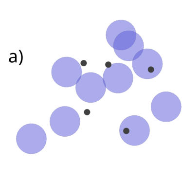
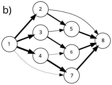
Figure 1: a) Coordination Navigation: selfish agents (purple) seek to reach rewards (black) whilst minimising contact with each other. b) Routing Networks: agents split their own commodity flow between edges in a network over a sequence of time-steps. Starting at a source (node 1) and arriving at a target node (8), paths that have more commodity incur higher congestion costs.

Continuous Stochastic Potential Games

We now introduce a new subset of SGs namely c-SPGs which is the framework of our approach.

Definition 1.

An SG is a c-SPG if for all states there exists a function $\phi:\mathcal{S}\times\boldsymbol{\mathcal{A}}\to\mathbb{R}$ such that the following holds for any $(a^{i},a^{-i}),(a^{\prime i},a^{-i})\in\boldsymbol{\mathcal{A}}$ where $a^{-i}_{t}:=(a^{1},\ldots a^{i-1},a^{i+1},\ldots,a^{N})$, $\forall i\in\mathcal{N},\forall s\in\mathcal{S}$:

$$R_{i}(s,(a^{i},a^{-i}))-R_{i}(s,(a^{\prime i},a^{-i}))$$

$$=\phi(s,(a^{i},a^{-i}))-\phi(s,(a^{\prime i},a^{-i})).$$ (1)

Condition (1) says that the difference in payoff from a deviation by one of the agents is exactly quantified by a global function $\phi$ that does not depend on the agent’s identity. We call $\phi$ the potential function or potential for short. The condition extends the notion of static one-shot potential games (PGs) (Monderer & Shapley, 1996b) to a continuous SG setting that now includes states and transition dynamics.

To complete the construction we introduce a condition which is a natural extension of PGs to state-based settings:

Definition 2.

A stage game $\mathcal{M}(s)$ is state transitive if there exists a $\phi:\mathcal{S}\times\boldsymbol{\mathcal{A}}\to\mathbb{R}$ s.th. $\forall(a^{i},a^{-i})\in\boldsymbol{\mathcal{A}},\forall i\in\mathcal{N},\forall s,s^{\prime}\in\mathcal{S}$:

$$R_{i}(s,(a^{i},a^{-i})) -R_{i}(s^{\prime},(a^{i},a^{-i}))$$

$$=\phi(s,(a^{i},a^{-i})) -\phi(s^{\prime},(a^{i},a^{-i})).$$ (2)

The intuition is that the difference in rewards for changing state is the same for each agent. Some classic examples of where state transitivity holds are anonymous games (Daskalakis & Papadimitriou, 2007), symmetric SGs (Jaśkiewicz & Nowak, 2018), team SGs (Cheng et al., 2017).

Our results are built under the assumption that state transitivity assumption holds.

Fig. 1 illustrates two examples of c-SPGs. For instance, in Coordination Navigation, one can verify that the state transitivity assumption is satisfied: a collection of agents seeks to arrive at some destination $x^{\star}\in\mathbb{R}^{p}$. Crucially, the agents must avoid colliding with other agents. Each agent’s value function is given by:

$$V_{i}^{\boldsymbol{\pi}} (\boldsymbol{x})=\frac{1}{2}\mathbb{E}\Bigg{[}\sum_{t=0}^{\infty}\gamma^{t}\Big{\{}K_{i}-\alpha\|x_{i,t}-x^{\star}\|^{2}$$

$${\color[rgb]{1,1,1}xxx} -\beta\sum_{j\in\mathcal{N}/\{i\}}(\|x_{i,t}-x_{j,t}\|^{2}+\epsilon)^{-1/2}-\|a_{i,t}^{T}-\rho\|_{M}^{2}\Big{\}}\Bigg{]}$$

where $\|\cdot\|$ and $\|\cdot\|_{M}$ are Euclidean and Mahalanobis norms respectively, $x_{i,t}\in\mathbb{R}^{p}$ is the position of agent $i$ at time $t\in\mathbb{N}$ and $\boldsymbol{x}_{t}=(x_{1,t},\ldots,x_{N,t})\in\mathbb{R}^{p}$; $c,\rho,H,\alpha,\beta\{K_{i}\}_{i\in\mathbb{N}}$ are constants and $a_{i,t}$ is vector representing the action taken by agent $i$. It can be readily verified that the game is potential with the following potential function: $\phi^{\boldsymbol{\pi}}(\boldsymbol{x})=-\alpha\|x-x^{\star}\|^{2}-\beta\sum_{j\in\mathcal{N}}\left(\|x-x_{j,t}\|^{2}+\epsilon\right)^{-1/2}+\beta c^{-2}-\|a^{T}-\rho\|^{2}$. Similarly, it can be readily verified that the game satisfies the state transitivity assumption.

In our Ablation experiments (see Sec. 6) we show that our method is able to tackle settings in which the potentiality and state transitivity conditions are mildly violated.

C-SPGs also hold in SGs in which the agents have the same reward functions (identical interest games)(Monderer & Shapley, 1996a) such as anonymous games (Daskalakis & Papadimitriou, 2007), team games (Wang & Sandholm, 2003) and mean field games (Mguni et al., 2018). Such SGs are widely used to study distributive systems and coordination problems in MAS such as Starcraft (Samvelyan et al., 2019) and Capture the Flag (Jaderberg et al., 2019). MARL frameworks such as COMA (Foerster et al., 2018), QMIX (Rashid et al., 2018) and QDPP (Yang et al., 2020) are fully cooperative settings and therefore fall within this category.

A key result we prove is that c-SPGs enjoy a dual representation as MDPs therefore enabling their solution to be computed by tackling MDPs. To construct a solution method for c-SPGs, we resolve a number of challenges: i) The first involves determining the dual MDP whose solution is to be learned through interaction with the environment. ii) The second involves developing a tractable learning procedure that ensures convergence to the game solution. To do this we develop a method that finds the solution of the dual MDP distributively, in doing so we also resolve the problem of combinatorial complexity that afflict MARL methods. iii) The method of determining the dual MDP (i)) can incur small errors. Our last challenge is to show that small errors in the construction of the dual MDP induce only small errors in the agents’ best response actions.

3.1 Link to Potential Games and Discussion

We briefly continue the discussion on related works with a relevant review of PGs. The first systematic treatment of PGs appeared in (Monderer & Shapley, 1996b) in a static setting. PGs constitute a fundamental building block of general-sum games - any general-sum game can be decomposed into two (strategic) parts; PGs and harmonic games (Candogan et al., 2011). PGs model many real-world scenarios including traffic network scenarios, network resource allocation (Zazo et al., 2015)) social conflicts (Lã et al., 2016) and consensus problems (Marden et al., 2009). PGs also encompass all team games and some zero-sum games (Balduzzi et al., 2018).

C-SPGs extend PGs to settings with dynamics and future uncertainty. This enables PGs to capture real-world scenarios that involve sequential decision-making and dynamics. Example of these settings traffic networks models, routing and packet delivery problems.

The analysis of dynamic PGs is extremely sparse and does not cover (reinforcement) learning settings in which the system is a priori unknown. In the direction of incorporating potentiality property within an SG, (González-Sánchez & Hernández-Lerma, 2013; Macua et al., 2018) consider an SG in which the potentiality property is imposed on the value functions which results in the need for highly restrictive assumptions. In (González-Sánchez & Hernández-Lerma, 2013) the SG is restricted to concave reward functions (in the state variable) and the transition function is required to be invertible (and known). These assumptions are generally incompatible with many MAS settings of interest. Similarly, (Macua et al., 2018) study a discrete Markov game in which the value function is assumed to satisfy a PG property. Their construction requires that the agents’ policies depend only on disjoint subcomponents of the state which prohibits non-local (strategic) interactions.

Very recently (Zhang et al., 2021) consider an SG setting in which all agents’ value functions are assumed to satisfy a global PG property, that is, the incentive of all agents to change their policies can now be expressed using a single global function. To construct this relationship using conditions on the stage game, in a later work (Leonardos et al., 2021) consider an SG setting and embed either of two properties into the game structure namely, an agent-independent transition assumption (C.1) or an equality of individual dummy term assumption (C.2). Using either of these conditions and the stage game PG condition (Condition (1)), they show that the PG condition can be extrapolated to a global PG condition on the value functions.

Conditions C.1. and C.2. in (Leonardos et al., 2021) impose heavy restrictions since Condition C.1. reduces the SG to a linear combination of normal form games and removes all planning aspects (hence extrapolating the potentiality of stage games to the agents’ value functions is deduced trivially). Condition C.2. restricts the noncooperative (strategic) interaction part of the game to a term that does not depend on the state or the agent’s own action. Moreover imposing condition C.2. produces an SG that is a special case of our SG (this can be seen using the equivalence expression in Lemma B (see Sec. H in Appendix) by setting $k(s)\equiv 1$ and restricting $h_{i}$ to depend only on other agents’ actions in the reward functions of our SG). Therefore, the generalisation of the PG condition to SGs in (Leonardos et al., 2021) requires strong limitations on the structure of the SG not present in our analysis.

With our new construction which has a PG at each stage game we show that the PG condition can be naturally extrapolated to the value functions of the SG. This provides verifiable assumptions on the game while imposing relatively weak assumptions on the SG in comparison to (Leonardos et al., 2021). With this we prove that the equilibrium of the SG can be found by merely solving an (unknown) MDP without imposing either state disjointness as in (Macua et al., 2018) or concavity as in (González-Sánchez & Hernández-Lerma, 2013).

4 Planning in c-Stochastic Potential Games

We now show that the stable point solution of a c-SPG can be computed tractably by solving a dual MDP with reward function $\phi$. This leads to a vast reduction in complexity for finding NEs in our c-SPG subclass of nonzero-sum. In what follows, we assume that the environment is known; in Sec. 5 we extend the analysis of this section to unknown environments. We defer the proofs of the results of the following sections to the Appendix.

As SGs are noncooperative settings, the solution cannot be described as an optimisation of a single objective. The appropriate solution concept is the following NE variant (Fudenberg & Tirole, 1991):

Definition 3.

A strategy profile $\boldsymbol{\hat{\pi}}=(\hat{\pi}_{i},\hat{\pi}_{-i})\in\boldsymbol{\Pi}$ is a Markov perfect equilibrium (MPE) if $\forall i\in\mathcal{N}$:

$v_{i}^{(\hat{\pi}_{i},\hat{\pi}_{-i})}(s)\geq v_{i}^{(\pi^{\prime}_{i},\hat{\pi}_{-i})}(s),\;\forall s\in\mathcal{S},\;\forall\pi_{i}^{\prime}\in\Pi_{i}$.

The condition characterises a fixed point in strategies in which no agent can improve their expected payoff by unilaterally deviating from their current policy. We denote the set of NE of $\mathcal{G}$ by $NE\{\mathcal{G}\}$. Finding NE of nonzero-sum SGs in general involves using fixed point methods which are generally intractable (Chen et al., 2009). Indeed, finding NE in SGs is PPAD complex (Polynomial Parity Arguments on Directed graphs) (Chen et al., 2009) for which brute force methods are intractable. Finding efficient solution methods for nonzero-sum SGs is an open challenge (Shoham & Leyton-Brown, 2008).

We now show that c-SPGs exhibit special properties that enable their NE to be computed tractably. In particular, we show that computing the NE of c-SPGs can be achieved by solving an MDP. With this, solving c-SPGs can be approached with stochastic approximation tools. We then present a new Q-learning variant that solves c-SPGs in polynomial time.

To begin, we construct the Bellman operator of $\mathcal{G}$. Let $g:\mathcal{S}\times\boldsymbol{\mathcal{A}}\to\mathbb{R}$ and $F:\mathcal{S}\to\mathbb{R}$, for any $s\in\mathcal{S}$ the Bellman operator of the game $\mathcal{G}$ is given by the following:

$$[T_{g}F](s):=\underset{\boldsymbol{a}\in\mathcal{A}}{\sup}\;[g(s,\boldsymbol{a})+\gamma\int_{s^{\prime}\in\mathcal{S}}ds^{\prime}P(s^{\prime};\boldsymbol{a},s)F[s^{\prime}]].$$

We now state our first key result which reveals a striking property of the c-SPG class of games:

Theorem 1.

Let $V:\mathcal{S}\times\boldsymbol{\mathcal{A}}\to\mathbb{R}$ be a test function, then $\mathcal{G}$ possesses a fixed point NE in pure (deterministic) Markov strategies characterised by:

$$\underset{k\to\infty}{\lim}T_{\phi}^{k}V^{\boldsymbol{\pi}}=\underset{{\boldsymbol{\hat{\pi}}}\in\boldsymbol{\Pi}}{\sup}V^{\boldsymbol{\hat{\pi}}},$$

where $\phi$ is the potential of $\mathcal{G}$.

The result states that the MPE of the game exist and in pure strategies and correspond to solution of a (dual) MDP $\mathscr{M}^{\dagger}:=\left\langle\phi,\times_{i\in\mathcal{N}}\mathcal{A}_{i},P,\mathcal{S},\gamma\right\rangle$. In fact, it is shown that any MPE is a local optimum of the value function associated to $\mathscr{M}$. The value function of $\mathscr{M}$ which we call the dynamic potential function (DPF), $B$, is constructed by $B^{\boldsymbol{\pi}}(s)=\mathbb{E}[\sum_{t=0}^{\infty}\gamma^{t}\phi(s_{t},\boldsymbol{a}_{t})|\boldsymbol{a}_{t}\sim\boldsymbol{\pi}]$, $\forall s\in\mathcal{S},\forall\boldsymbol{\pi}\in\boldsymbol{\Pi}$.

The theorem is proven inductively within a dynamic programming argument to extrapolate the potentiality property to the entire SG then showing $\mathcal{G}$ is continuous at infinity.

Theorem 1 enables us to compute the MPE by solving an MDP, a task which can be performed in polynomial time. Moreover, Theorem 1 enables a Q-learning approach (Bertsekas, 2012) for finding the MPE of the game. The following fitted Q-learning method computes the approximate $B$ function and the corresponding optimal policy for each agent.

First, let us define by

$$Y_{l_{k}}(s_{l_{k}},\boldsymbol{a}_{l_{k}},s^{\prime}_{l_{k}}):=\phi_{l_{k},\hat{\rho}}(s_{l_{k}},\boldsymbol{a}_{l_{k}})+\gamma\underset{\boldsymbol{a^{\prime}}}{\sup}\;\mathbb{E}_{\mathbb{P}}\left[\hat{B}_{l}\right](s^{\prime}_{l_{k}},\boldsymbol{a^{\prime}})$$ (3)

At each iteration $k=0,1,\ldots$ we solve the minimisation:

$$F_{l}\in\underset{\mathcal{F}\in\mathcal{H}}{\arg\inf}\sum_{l_{k}=1}^{n_{k}}\left(Y_{l_{k}}(s_{l_{k}},\boldsymbol{a}_{l_{k}},s^{\prime}_{l_{k}})-\left[\mathcal{F}\right](s_{l_{k}},\boldsymbol{a}_{l_{k}})\right)^{2}$$ (4)

0:  discount factor $\gamma$ and PF $\phi$.

1:  for $k\in{0,1,2,\cdots}$ do

2:     for $i\in\mathcal{N}$ do

3:        Set the local target $Y_{l_{k}}$ by (3)

4:        Update $F$ by minimizing Eq. (4)

5:     end for

6:  end for

6:  $F,(\pi_{i}^{k})_{i\in\mathcal{N}}$.

Algorithm 1 SPotQ: Stochastic POTential Q-Learning

The minimisation seeks to find the optimal action-value function $Q^{\star}$. Using this, we can construct our SPotQ algorithm that works by mimicking value iteration. By Theorem 1, the algorithm converges to the MPE of the game.

Theorem 1 does not establish uniqueness of $B$ which could lead to ambiguity in the solution. The following result reduces the set of candidates to a single family of functions:

Lemma 1.

If $B_{1},B_{2}$ are value functions of the dual MDP $\mathcal{M}^{\dagger}$ then $(B_{1}^{\boldsymbol{\pi}}-B_{2}^{\boldsymbol{\pi}})(s)=c,\forall\boldsymbol{\pi}\in\boldsymbol{\Pi},\forall s\in\mathcal{S}$ where $c\in\mathbb{R}$

Therefore, the set of candidate functions are limited to a family of functions that differ only by a constant.

Computing the Potential Function $\phi$

Theorem 1 requires knowledge of $\phi$. Existing methods to find $\phi$ in PGs e.g. MPD method (Candogan et al., 2013) are combinatorial in actions and agents. Indeed, directly applying (1) to compute $\phi$ requires checking all deviations over pure strategies (deterministic policies) which is expensive since it involves sweeping through the joint action space $\boldsymbol{\mathcal{A}}$. We now demonstrate how to compute $\phi$ while overcoming these issues by transforming (1) into a differential equation. To employ standard RL methods we require parameterised policies and, in anticipation of tackling an RL setting we extend our coverage to parameterised stochastic policies.

Proposition 1.

In any c-SPG the following result holds $\forall s\in\mathcal{S},\forall\boldsymbol{a}\in\mathcal{A}$, $\forall(\boldsymbol{\eta}^{i},\boldsymbol{\eta}^{-i})\in\boldsymbol{E}^{ps}$:

$$\mathbb{E}_{\boldsymbol{\pi}(\boldsymbol{\eta})}\left[\frac{\partial\ln{\pi_{i,\boldsymbol{\eta}^{i}}}}{\partial\boldsymbol{\eta}^{i}}\left(\frac{\partial}{\partial a^{i}}+\frac{\partial}{\partial s}\right)(R_{i}-\phi)(s,\boldsymbol{a})\right]=\boldsymbol{0}.$$ (5)

The PDE serves as an analogue to the PG condition (1) which now exploits the continuity of the action space and the fact that they agents’ actions are sampled from stochastic policies. Therefore Prop. 1 reduces the problem of finding $\phi$ to solving a PDE.

So far we have considered a planning solution method that solves the game when the agents reward functions are known upfront. In Sec 5, we consider settings in which the reward functions and the transition function are a priori unknown but the agents observe their rewards with noisy feedback.

5 Learning in c-Stochastic Potential Games

In RL, an agent learns to maximise its total rewards by repeated interaction with an unknown environment. The underlying problem is typically formalised as an MDP (Sutton & Barto, 2018). MARL extends RL to a multi-player setting (Yang & Wang, 2020). The underlying problem is modelled as an SG in which the rewards of each agent and transition dynamics are a priori unknown.

We have shown the MPE of a c-SPG can be computed by solving a Markov team game $\mathscr{M}^{\dagger}$, an SG in which all agents share the same reward function $\phi$. We now discuss how to solve $\mathscr{M}^{\dagger}$ from observed data in unknown environments (i.e. if $P,\{R_{i}\}$ are not known). Additionally, we discuss our approach to enable easy scaling in the number of agents (and avoid combinatorial complexity) using distributive methods.

The scheme can be summarised in the following steps:

i) Compute the potential estimate $\hat{\phi}$ by solving the PDE in Prop. 1 using a distributed supervised learning method.

ii) Solve the team game $\hat{\mathscr{M}}^{\dagger}:=\langle\mathcal{N},\mathcal{S},\boldsymbol{\mathcal{A}},P,\hat{\phi},\gamma\rangle$ with a distributed actor-critic method. The critic is updated with a distributed variant of the fitted Q-learning method in Sec. 4.

5.1 Learning the Potential Function $\phi$

Though Prop. 1 reveals that $\phi$ can be found by solving a PDE, it involves evaluations in pure strategies which can be costly. Moreover, the result cannot be applied directly to estimate $\phi$ since the agents sample their rewards but not $\phi$.

We now show how each agent can construct an approximation of $\phi$ in a way that generalises across actions and states by sampling its rewards. First, we demonstrate how the potential condition (1) can be closely satisfied using almost pure strategies. The usefulness of this will become apparent when we solve the PDE in Prop. 1 to find $\phi$.

Lemma 2.

Let $F$ be a bounded and continuous function and let $\Delta F(s_{t},(a^{i}_{t},a^{\prime i}_{t}),a^{-i}_{t}):=F(s_{t},(a^{\prime i}_{t},a^{-i}_{t}))-F(s_{t},(a^{i}_{t},a^{-i}_{t}))$ then there exists $c>0$ such that

$$\left|\Delta F(s_{t},(a^{i}_{t},a^{\prime i}_{t}),a^{-i}_{t})-\Delta F(s_{t},(\pi_{i},\pi^{\prime}_{i}),\pi_{-i}))\right|\leq c\|F\|_{\infty}\hat{\sigma}_{\epsilon}^{2}$$

where the policy $\pi_{i,\epsilon}$ is a nascent delta function and $\hat{\sigma}^{2}_{\epsilon}:=\max\{\rm{Var}(\pi_{i}),\rm{Var}(\pi^{\prime}_{i})\}$.

Since the bound approaches $0$ in the limit as policies become pure strategies, the potential condition (5) is closely satisfied in nascent stochastic policies.

We now put Lemma 2 to use with a method to compute $\hat{\phi}$ that inexpensively solves the PDE condition (5) over the policy parameter space $\boldsymbol{E}$. Indeed, thanks to Lemma 2, we can learn $\phi$ through an optimisation over $\boldsymbol{E}$. The method uses a PDE solver over a set of randomly sampled points across $\boldsymbol{E}\times\mathcal{S}$ using the observed data $\{(s_{k},\boldsymbol{a}_{t},(r_{1,k},\ldots,r_{N,k}))\}_{k\geq 0}$ where $r_{i,k}\sim R_{i}(s_{k},\boldsymbol{a}_{k})$.

Therefore, define by:

$$g^{i}(s,{\boldsymbol{\eta}},\hat{\phi}):=\nabla_{\boldsymbol{\eta}^{i}}\ln{\pi_{\epsilon,i}(a^{i}|s;\boldsymbol{\eta})}\left(\frac{\partial}{\partial a^{i}}+\frac{\partial}{\partial s}\right)[R_{i}-\hat{\phi}](s,\boldsymbol{a})$$

where $\boldsymbol{\pi}_{\epsilon}(\boldsymbol{a}|s;\boldsymbol{\eta}):=\pi_{\epsilon,i}(a^{i}|s;\boldsymbol{\eta}^{i})\pi_{\epsilon,-i}(a^{-i}|s;\boldsymbol{\eta}^{-i})$.

Following Prop. 1 we consider the following problem to compute $\hat{\phi}$:

$$\underset{\boldsymbol{\rho}\in\mathbb{R}^{k}}{\min}\|G(s,{\boldsymbol{\eta}};\hat{\phi}_{\boldsymbol{\rho}})\|^{2}_{\boldsymbol{E}\times\mathcal{S},\nu},$$ (6)

where $G(s,\boldsymbol{\eta};\hat{\phi}):=[g^{1}(s,\boldsymbol{\eta};\hat{\phi}),\ldots,g^{N}(s,{\boldsymbol{\eta}};\hat{\phi})]^{T}$ and $\|f(y)\|^{2}:=\int_{Y}|f(y)|^{2}\nu(y)dy$ and $\nu(y)$ is a positive probability density on $Y$ and $\boldsymbol{\rho}\in\mathbb{R}^{k}$ are parameters. The optimisation performs evaluations in mixed strategies which is computationally inexpensive. Using a weighted exponential sum method (Chang, 2015), the objective reduces to a least squares problem on a single objective $G(s,\boldsymbol{\eta},\boldsymbol{\rho}):=N^{-1}\sum_{i\in\mathcal{N}}\left(g^{i}(s,\boldsymbol{\eta},\hat{\phi}_{\boldsymbol{\rho}^{i}})\right)^{2}$. The optimisation can be solved with a function approximator on $\hat{\phi}_{\boldsymbol{\rho}}$ e.g. a deep neural network (NN). Under mild conditions (Bertsekas & Tsitsiklis, 2000) the method converges to a critical point of $G$, that is $\underset{n\to\infty}{\lim}\nabla_{\boldsymbol{\rho}}G=0$. We defer the details of the method to the the Appendix.

Actor-Critic Method

We now return to tackling the problem of solving the team game $\hat{\mathscr{M}}^{\dagger}:=\langle\mathcal{N},\mathcal{S},\boldsymbol{\mathcal{A}},P,\hat{\phi},\gamma\rangle$. To enable the method to scale and handle continuous actions, we adapt the fitted Q-learning method in Sec. 4 to an actor-critic method (Konda & Tsitsiklis, 2000) for which each agent learns its own policy $\pi_{i,\eta_{i}}$ using the estimate of $B$. The policy parameter $\eta_{i}$ of the policy at the $k^{th}$ iteration is updated through sampled deterministic policy gradients (DPGs) (Silver et al., 2014):

$$\nabla\eta_{i}\hat{B}^{(\pi^{k}_{i,\eta_{i}},\pi^{k}_{-i,\eta_{-i}})}\left(s_{l_{k}}\right)$$

$$\approx\frac{1}{L}\sum_{l=1}^{L}\nabla_{\eta_{i}}\pi_{i,\eta_{i}}\left(\cdot|s_{l_{k}}\right)\nabla_{a^{i}_{l_{k}}}F_{k}\left(s_{l_{k}},\boldsymbol{a}_{l_{k}}\right)\Big{|}_{a^{i}_{l_{k}}\sim\pi^{k}_{i,\eta_{i}}}$$ (7)

Equation (7) describes the actor update via a DPG. The complete process is described in Algorithm 1. It involves two optimisations in sequence: the agents individually compute the approximation $\hat{\phi}$ which is then used for computing $\hat{B}$, which approximates the optimal value function $B$ by a Q-learning + decentralised DPG method and outputs each agent’s MPE policy. Crucially the method avoids optimisations over the joint space $\times_{i\in\mathcal{N}}\mathcal{A}_{i}$ enabling easy scaling (in the number of agents) in this component of the algorithm.

0:  discount factor $\gamma$, DPF and PF approximation maps $F,P_{\boldsymbol{\rho}}\in\mathcal{H}$ (resp.) ($\boldsymbol{\rho}\in\mathbb{R}^{k}$).

1:  for $k\in{0,1,2,\cdots}$ do

2:     Using $(\pi_{i}^{k})_{i\in\mathcal{N}}$ to rollout, collect the trajectory data and save it in the buffer $\mathcal{D}$.

3:     for $i\in\mathcal{N}$ do

4:        // Learn the potential function $\hat{\phi}$

5:        Sample a random minibatch of $L$ samples $\{(s_{l_{t}},(a^{i}_{l_{t}})_{i\in\mathcal{N}},s_{l_{t+1}},(r^{i}_{l_{t}})_{i\in\mathcal{N}}\}$ from $\mathcal{D}$.

6:        Compute $\hat{\phi}$ by solving Expression (6)

7:        // Compute the value function $\hat{B}$

8:        Set the local target $Y_{l_{k}}$ by (3)

9:        Update the shared critic $F$ by minimizing Eq. (4)

10:        // Learn the individual policy

11:        Update the policy by minimizing Eq. (7)

12:     end for

13:  end for

13:  $F,(\pi_{i}^{k})_{i\in\mathcal{N}}$.

Algorithm 2 SPot-AC: Stochastic POTential Actor-Critic

Scaling in $N$ using Consensus Optimisation
Although the above method represents progress for solving SGs, a scalability issue remains since estimating $\hat{\phi}$ involves a computation over the joint space $\boldsymbol{E}$. This becomes increasingly expensive with large numbers of agents. We now devise a fully distributed version of the method that scales with the number of agents. In this version, each agent $i$ constructs an independent estimate of $\hat{\phi}$ by sampling across $E_{i}\times\mathcal{S}$ at each step using only its own observed data $\{(s_{k},\boldsymbol{a}_{t},r_{i,k})\}_{k\geq 0}$. The method includes a consensus step that enables $\hat{\phi}$ (and hence $\hat{B})$ to be accurately computed efficiently in a fully distributed fashion (Tutunov et al., 2019).

To enable efficient scaling with the number of agents, we use distributed optimisation (DO) with consensus (Nedic & Ozdaglar, 2009) to find $\hat{\phi}$. Each agent produces its own estimate $\hat{B}$ based on its observed rewards. DO methods efficiently solve large scale optimisation problems (Macua et al., 2010) and yields two major benefits:
i) efficiency: computing $\phi$ uses feedback from all agents’ reward samples.
ii) consensus on Q: agents learn $\phi$ distributively but have identical Q iterates (for computing $\hat{B}$).

The common objective which each agent solves individually, is expressed with a set of local variables $\{\rho_{i}\}_{i\in\mathcal{N}}$ and a common global variable $z$:

${\rm minimise}\;\;\bar{G}(s,\boldsymbol{\rho})=N^{-1}\sum_{i\in\mathcal{N}}(g^{i}(s,\boldsymbol{\rho}^{i}))^{2}$

s.t. $\boldsymbol{\rho}^{i}-z=0,\quad i=1,\ldots,N,$
where the gradient descent is according to: $\boldsymbol{\rho}^{i}_{n}=\boldsymbol{\rho}^{i}_{n-1}-\alpha\nabla g^{i}(s,\boldsymbol{\rho}^{i})$ for some step size $\alpha>0$. Note that the constraint prevents convergence to any $R_{i}$.

The algorithm works by constructing an estimate $\hat{\phi}$ then solving $\mathscr{M}^{\dagger}$ in a distributed fashion allowing the method to scale with the number of agents.

Algorithm Analysis

Our SPot-AC algorithm inherits many useful properties of Q-learning (Antos et al., 2008). Nevertheless, it is necessary to ensure the output of the algorithm still yields good performance when the supervised learning approximation of $\mathcal{M}^{\dagger}$ has small errors. We now analyse the SPot-AC algorithm and show that provided errors in approximating $\mathcal{M}^{\dagger}$ are small the error in the algorithm output is also small.

Our first result bounds the error on the estimate for the DPF from using the approximation method for $\hat{\phi}$.

Proposition 2.

Define by the following $F_{i}(s,\boldsymbol{\eta},\rho):=\int_{\boldsymbol{\mathcal{A}}}\boldsymbol{\pi}_{\epsilon}(\boldsymbol{da},\boldsymbol{\eta},s)\frac{\partial}{\partial\eta_{i}}\pi_{i,\epsilon}(a^{i},\eta_{i},s)\nabla F_{\rho}(s,\boldsymbol{a})$ and $U(s,\boldsymbol{\eta},\rho):=\int_{\boldsymbol{\mathcal{A}}}\boldsymbol{\pi}_{\epsilon}(\boldsymbol{da},\boldsymbol{\eta},s)\frac{\partial}{\partial\eta_{i}}\pi_{i,\epsilon}(a^{i},\eta_{i},s)\nabla R_{i}(s,\boldsymbol{a})$ then the following bound holds for some $c>0$:

$$\sum_{i\in\mathcal{N}}\left\|F_{i}(s,\boldsymbol{\eta},\rho)-U(s,\boldsymbol{\eta})\right\|\leq cN^{2}\epsilon^{2},$$

where $\epsilon$ is the approximation error from the SL procedure.

Our next result ensures that if the estimates of $\phi$ have only small errors, SPot-AC generates policy performances that closely match that of the MPE policies.

Proposition 3.

Define by $B_{\epsilon}^{\boldsymbol{\tilde{\pi}}}=\underset{k\to\infty}{\lim}T_{\phi_{\epsilon}}^{k}B^{\boldsymbol{\pi}}$ and let the policy $\boldsymbol{\hat{\pi}}$ be an MPE strategy i.e. $\boldsymbol{\hat{\pi}}\in NE\{\mathcal{G}\}$ (so that $\underset{k\to\infty}{\lim}T_{\phi}^{k}B^{\boldsymbol{\pi}}=B^{\boldsymbol{\hat{\pi}}}$) then for any $\epsilon>0$ the following holds:

$$\|B^{\boldsymbol{\hat{\pi}}}-B_{\epsilon}^{\boldsymbol{\tilde{\pi}}}\|\leq(2-\gamma)(1-\gamma)^{-1}\epsilon,$$

whenever $\|\phi^{\epsilon}-\phi\|<\epsilon$.

The result ensures that given close approximations of $\phi$ SPot-AC in turn yields outputs close to $B^{\star}$. The result exploits the fact that the dual MDP $\mathcal{M}$ of Theorem 1 exhibits a continuity property so that small errors in the approximation of $\phi$ and $B$ incur only small changes to the MPE of $\mathcal{G}$.

6 Experiments

We evaluate SPot-AC in three popular multi-agent environments: the particle world (Lowe et al., 2017), a network routing game (Roughgarden, 2007) and a Cournot duopoly problem (Agliari et al., 2016). These environments have continuous action and state spaces, and the agents seek to maximise their own interest e.g. reaching target without collisions on particle world and minimising the cost for transporting commodity on routing game. To solve these problems successfully, the agents must learn Markov perfect equilibrium policies in order to respond optimally to the actions of others.

We consider two groups of state-of-the-art MARL baselines that handle continuous actions. The first group use individual rewards for learning: MADDPG (Lowe et al., 2017) and DDPG (Lillicrap et al., 2015). The second group use the collective rewards of all agents: COMIX and COVDN (de Witt et al., 2020). Further details are in the Appendix.

We use two evaluation metrics:
Exploitability (Davis et al., 2014) describes how much additional payoff players can achieve by playing a best-response policy $\operatorname{BR}$ (defined in the Appendix). It measures the proximity of the agents’ policies to the MPE strategy, defined as $\delta=\frac{1}{N}\sum_{i}(u_{i}(\pi^{-i},\operatorname{BR}(\pi^{-i}))-u_{i}(\pi))$.
Social welfare is the collective reward of all agents: $r=\sum_{i=1}^{N}r_{i}$, this is most relevant in tasks such as team games, where agents seek to maximise total reward.

Ablation Studies

To test the robustness of SPot-AC and the baselines, we perform a set of ablation studies within routing games.
Ablation 1 analyses SPot-AC in SGs that progressively deviate from c-SPGs, showing that SPot-AC can handle SGs that mildly violate the c-SPG conditions (i.e. the potentiality requirement).
Ablation 2 analyses SPot-AC in SGs that progressively deviate from team games but retain the potential game property. We demonstrate that, unlike other methods, SPot-AC is able to converge to the Markov Perfect Equilibrium in non-cooperative SGs. We also report results on the classic Cournot Duopoly and show convergence of SPot-AC to NE.

Non-atomic Routing Games involve a set of $N$ selfish agents seeking to transport their commodity from a source node to a goal node in a network. This commodity can be divided arbitrarily and sent between nodes along edges.

At each time step, each agent has a distribution of commodity over the nodes of the graph. It assigns a fraction of its commodity in each node to travel along the edges emerging from those nodes. There are multiple agents (given by $N\in\{2,4,6,8\}$), using the same network (number of nodes $K\in\{20,40\}$) and agents pay a cost related to the total congestion of every edge at each time step. We design the game so that the MPE is socially efficient, i.e. playing an MPE strategy leads to high individual returns. We repeat the experiments for 5 independent runs and report the mean and standard deviation of the rewards. Further details on the settings can be found in Appendix.

Results

Exploitability: We test SPot-AC in a simple Braess’ paradox game. The exploitability of SPot-AC (Fig. 2) quickly converges to close to $0$, indicating it learns NE policies (negative values are due to the fact that we are approximating best-responses). In contrast, the high exploitability values of existing MARL methods indicate that they fail to converge to NE policies. The algorithms that involve reward sharing (COMIX, COVDN) attempt to maximise social welfare, which is incompatible with this non-cooperative setting, so can be exploited by a best-response strategy.

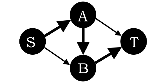
(a) SPot-AC’s policy on Braess’ paradox

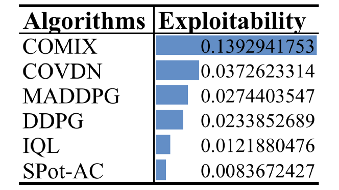
(b) Exploitability of different methods.

Figure 2: Results of exploitability. (a) a visualization of learned policy flows by SPot-AC. (b) Exploitability results of all methods.

Social welfare: In the cooperative, non-atomic routing game environment, we see in Fig. 3, using SPot-AC (orange), each agent learns how to split their commodity $G$ in a way that maximises rewards (minimises costs) and matches the shared reward baselines. Conversely, MADDPG (orange) and DDPG (blue) yield low rewards with high variance.

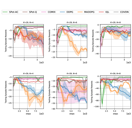
Figure 3: Top Average agent returns in Network with $N=4,6,8$ agents, $K=20$ nodes. Bottom Average agent returns in Network with $N=4,6,8$ agents, $K=59$ nodes.

Coordination Navigation An OpenAI Multi Agent Particle Environment task (Lowe et al., 2017) involves $n$ agents and $n$ landmarks. Each agent must reach the target while avoiding collisions with other agents and fixed landmarks. Agents can observe the relative positions of other agents and landmarks, and have five actions {up, down, left, right, stay}. The reward is calculated as the agent’s distance to each landmark with penalties for collisions with other agents.

This is a non-cooperative SG, so we compare SPot-AC to DDPG and MADDPG, algorithms that are able to learn policies in which agents can act selfishly. We perform the exploitability analysis as above. Fig. 4 shows SPot-AC achieves the best performance in terms of minimum distance to target and number of collisions, demonstrating that SPot-AC enables agents to learn to coordinate while pursuing their own goals.

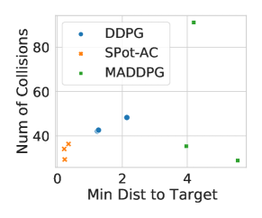
Figure 4: Coordination Navigation problem.

7 Conclusion

In this paper, we describe the first MARL framework that tackles MAS with payoff structures beyond zero-sum or team games. In doing so, the results we establish pave the way for a new generation of solvers that are able to tackle classes of SGs beyond cases in which the payoff structures lie at extremes. Therefore, the results of this paper open the door for MARL techniques to address a wider range of multi-agent scenarios. By developing theory that shows a class of SGs, namely c-SPGs have a dual representation as MDPs, we showed that c-SPGs can be solved by MARL agents using a novel distributed method which avoids the combinatorial explosion therefore allowing the solver to scale with the number of agents. We then validated our theory in experiments in previously unsolvable scenarios showing our method successfully learns MPE policies in contrast to existing MARL methods.

The Supplementary material is arranged as follows: first, in Sec. A we give a description of the experimental details and report the hyperparameter values used in our experiments. In Sec. B, we give a detailed discussion of our ablation studies. In Sec. C, we give results of our analysis on a static noncooperative game namely Cournot duopoly problem and in Sec. D we perform an study of the problem and verify our solution analytically. In Sec. E, we give additional details on our supervised learning method to compute the potential function. In Sec. F, we give additional details on our distributed learning method using consensus optimisation required to compute the potential function distributively. In Sec. G, we outline some of the additional notation and detail the technical assumptions used in the proofs of our results which are contained in Sec. H which concludes the supplementary material.

Appendix A Experiment Details & Hyperparameter Settings

The settings for all methods are the same, except for the stated cases that use a shared critic. The optimiser is set to Adam for all methods reported. The learning rates for actors and critics are 1e-4 and 1e-3 respectively. Both actors and critics consist of four fully connected layers with dimensions of [64,64,64,$n_{act}$].

In the table below we report all hyperparameters used in our experiments. Hyperparameter values in square brackets indicate range of values that were used for performance tuning.

Setting	Value
Clip Gradient Norm	1
Discount factor $\gamma_{E}$	0.99
$\lambda$	0.95
Learning rate	$1$x$10^{-4}$ for actor and $1$x$10^{-3}$ for critic
Batch size	256
Buffer size	4096
Policy architecture	MLP
Number of parallel actors	1
Optimization algorithm	Adam
Rollout length	1000*[10, 20]

Appendix B Ablation Studies

Our method allows MARL agents to solve noncooperative SGs within the SPG subclass. In this section, we analyse the behaviour of our method compared against existing MARL baselines in scenarios that range from team (cooperative) SG settings to noncooperative games outside of SPGs. In doing so, we examine their performance when the SPG assumptions are violated and show that SPot-AC is still able to perform well when the PG condition (Equation (1)) is mildly violated. Additionally, in these settings we also compare the performance of SPot-AC in cooperative settings which are the degenerate case of SPGs.

As in Section 6 (within the main body), we consider a stochastic network routing game which has both continuous action and state spaces and is a nonzero sum game (neither team-based nor zero-sum) which represents a challenge for current MARL methods. As in the Network routing games considered in Section 6, we restrict our attention to networks that have efficient NE. In such network structures, playing an NE (best-response) strategy leads to a higher total return for the (self-interested) agent. For these networks, the average return for an agent serves as a measure the performance of the different algorithms.

Figure 5: Selfish routing network with 200 nodes.

B.1 Non-Cooperative, Stochastic Potential Game Ablation Study

Fig. 5 demonstrates the large network used in experiments. The class of potential games includes all team-games as a subclass, i.e. every team game is a potential game, and some but not all non-cooperative games are potential. In this ablation study, we examine the performance of SPot-AC against other baselines in stochastic potential but non-cooperative games.

To do this, using Lemma C, we know that, in any potential game, the reward function $R_{i}:\mathcal{S}\times\left(\times\mathcal{A}_{i\in\mathcal{N}}\right)\to\mathbb{R}$ for any agent $i\in\mathcal{N}$ can be decomposed into two components: the team game component $J:\mathcal{S}\times\left(\times\mathcal{A}_{i\in\mathcal{N}}\right)\to\mathbb{R}$ (i.e. function that all agents seek to maximise) and a strategic (non-cooperative) component which is specific to each agent $L_{i}:\mathcal{S}\times\left(\times\mathcal{A}_{i\in\mathcal{N}/{\{i\}}}\right)\to\mathbb{R}$. We now study a set of games in which each agent’s reward function has the following form:

$$R_{i}(s,(a_{i},a_{-i}))=\underbrace{J(s,(a_{i},a_{-i}))}_{\text{Team game reward}}+c\underbrace{L_{i}(s,a_{1},\ldots{\color[rgb]{1,0,0}a_{i-1},a_{i+1}},\ldots,a_{N})}_{\text{Non-cooperative part}}$$ (8)

The value of the constant $c\in\mathbb{R}$ determines the contribution of the non-cooperative, strategic component. For $c=0$, the game is a team game and as $c\to\infty$ the non-cooperative component of the game dominates.

As can be seen in the plots, SPot-AC has better average return compared to the DDPG-based algorithms, whose performance degrades most due to their team-game requirement. COMIX and COVDN achieve similar levels of performance.

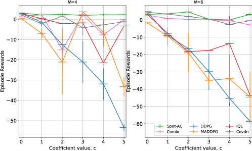
Figure 6: Results of the training curves for the non-cooperative, potential non-atomic routing game when the number of agents $N=4,6$, with $c=0,1,2,3,4,5$.

B.2 Non-cooperative, Non-Potential Stochastic Game Ablation Study

Extending the ablation studies of the previous section, we examine the performance of SPot-AC in games that are both non-cooperative and not potential. We parameterise the agents’ reward function for the congestion game as follows:

$$R_{i}(s,(a^{i},a^{-i}))=\underbrace{r_{i}(s,(a^{i},a^{-i}))}_{\text{potential reward function}}+\hskip 5.69054ptc\underbrace{J(s,(a^{i},a^{-i}))}_{\text{non-potential contribution}},\qquad\forall s\in\mathcal{S},\forall(a^{i},a^{-i})\in\boldsymbol{\mathcal{A}}.$$

The functions $r_{i}$ are those from the original (potential) congestion game (1). $J$ is a generic non-potential reward function. $c=0$ corresponds to a potential game, and as $c\to\infty$ the non-potential component of the game dominates.

Fig. 7 shows the results of this ablation study in a network routing game with 4 agents. We see that SPot$-$ACis able to handle small deviations (small $c$) from the potential requirements, but performance degrades for larger values. It again outperforms the DDPG baselines, whose performance degrades rapidly with increasing values of the ablation parameter.

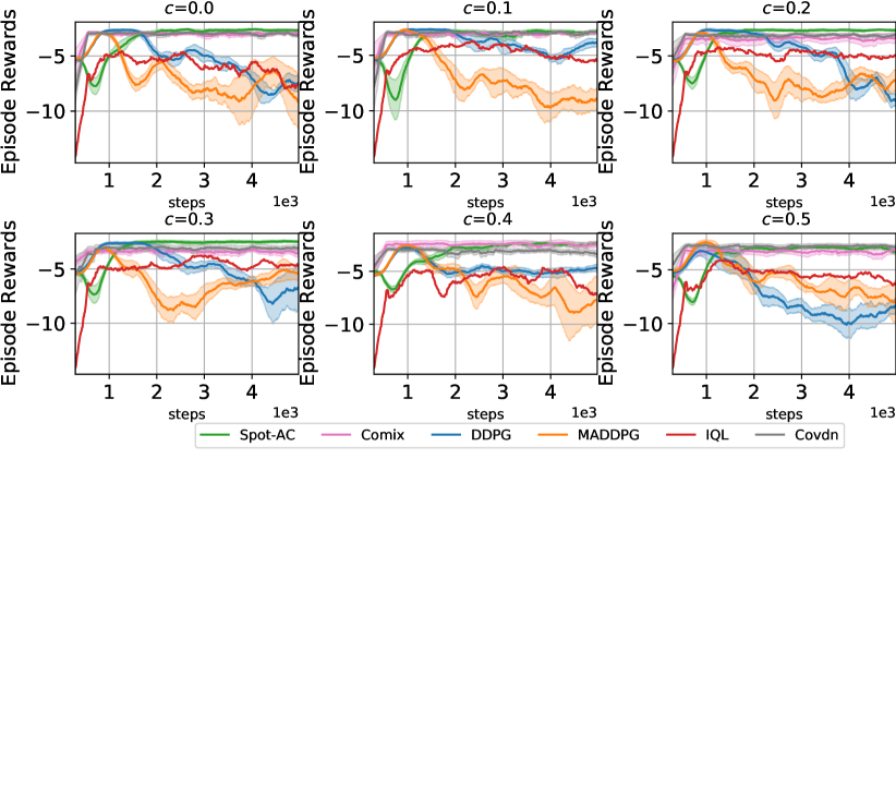
Figure 7: Results of the training curves for non-cooperative, non-potenial, non-atomic routing game when number of agents $N=4$, coefficients $c=0.0-0.5$.

Appendix C Cournot Duopoly Problem

Cournot Duopoly is a classic static game (Monderer & Shapley, 1996b) that models the imperfect competition in which multiple firms compete in price and production to capture market share. Since the firms’ actions are continuous variables, the game is a continuous action setting. It is a nonzero sum game (neither team-based nor zero-sum) which represents a challenge for current MARL methods. Let $a_{i}\in[-A_{i},A_{i}]$ where $A_{i}\in\mathbb{R}_{>0}$ which represent the set of actions for Firm $i\in\{1,2\ldots,N\}:=\mathcal{N}$. Let $\alpha,\beta,\gamma\in\mathbb{R}_{>0}$ be given constants, each firm i’s reward (profit) is $R_{i}(a_{i},a_{-i})=a_{i}(\alpha-\beta\sum_{i\in\mathcal{N}}a_{i})-\gamma a_{i}$. We set $A_{i}=1,\forall i\in\mathcal{N}$ and $\alpha=\gamma=1,\beta=-1$.

Appendix D Analytic Example: Cournot Duopoly

Reward functions

Let $a_{1}\in[-A_{1},A_{1}]$ and $a_{2}\in[-A_{2},A_{2}]$ where $A_{1},A_{2}\in\mathbb{R}_{>0}$ which represent the actions for Firm 1 and Firm 2 respectively.

Also let $\alpha,\beta,\gamma\in\mathbb{R}_{>0}$ be given constants.

$$R_{i}(a_{1},a_{2})=a_{i}(\alpha-\beta(a_{1}+a_{2}))-\gamma a_{i}$$ (9)

Cournot Potential Function ($N=2$ Agents)

$$\phi(a_{1},a_{2})=\alpha(a_{1}+a_{2})-\beta(a_{1}^{2}+a_{2}^{2})-\beta a_{1}a_{2}-\gamma(a_{1}+a_{2})+k$$ (10)

where $k\in\mathbb{R}$ is an arbitrary constant.

D.1 Cournot Duopoly with $N>2$ Agents

Reward functions

Let $a_{i}\in[-A_{i},A_{i}]$ where $A_{i}\in\mathbb{R}_{>0}$ which represent the actions for Firm $i$, $i\in\{1,2\ldots,N\}$.

Also let $\alpha,\beta,\gamma\in\mathbb{R}_{>0}$ be given constants.

$$R_{i}(a_{i},a_{-i})=a_{i}(\alpha-\beta\sum_{i\in\mathcal{N}}a_{i})-\gamma a_{i}$$ (11)

Cournot Potential Function ($N\geq 2$ Agents)

$$\phi(a_{i},a_{-i})=\alpha\sum_{i\in\mathcal{N}}a_{i}-\beta\sum_{i\in\mathcal{N}}a_{i}^{2}-\beta a_{i}\sum_{j\in\mathcal{N}/\{i\}}a_{j}-\gamma\sum_{i\in\mathcal{N}}a_{i}+k$$ (12)

where $k\in\mathbb{R}$ is an arbitrary constant.

Derivatives

$$\frac{\partial R_{i}(a_{i},a_{-i})}{\partial a_{i}}=\alpha-\beta\sum_{i\in\mathcal{N}}a_{i}-\beta a_{i}-\gamma$$ (13)

$$\frac{\partial\phi(a_{i},a_{-i})}{\partial a_{i}}=\alpha-2\beta a_{i}-\beta\sum_{j\in\mathcal{N}/\{i\}}a_{j}-\gamma$$ (14)

D.2 Analytic Verification of our Method

In this section, we validate that the optimisation in Sec. 5.1 yields the correct results. To do this, we derive analytic expressions for $\phi$ and show that the solution of the optimisation in Sec. 5.1 coincides with this solution. Recall that our proposition says that:

$$\mathbb{E}_{(a^{i},a^{-i})\sim(\pi_{i}(\eta^{i}),\pi_{-i}(\eta^{-i}))}\left[\frac{\partial}{\partial\eta^{i}}\ln{[\pi_{i}(a^{i}|s;\eta^{i})]}\left(\frac{\partial}{\partial a^{i}}R_{i}(s,a^{i},a^{-i})-\frac{\partial}{\partial a^{i}}\phi(s,a^{i},a^{-i})\right)\right]=\boldsymbol{0},$$ (15)

We first want to check that any PF in (10) solves (15), indeed:

For $\implies$ we find that

$$\frac{\partial}{\partial a^{i}}R_{i}(\cdot,a^{i},a^{-i}) =\alpha-\beta(a_{1}+a_{2})-\beta a_{i}-\gamma$$

and

$$\frac{\partial}{\partial a^{i}}\phi(\cdot,a^{i},a^{-i}) =\alpha-2\beta a_{i}-\beta a_{j}-\gamma$$

$$=\alpha-\beta(a_{1}+a_{2})-\beta a_{i}-\gamma$$

and hence verify:

$$\frac{\partial}{\partial a^{i}}\phi(\cdot,a^{i},a^{-i})-\frac{\partial}{\partial a^{i}}R_{i}(\cdot,a^{i},a^{-i})=0$$

so that any $\phi$ in (10) is a candidate solution to (15). Indeed, we observe that

$$\frac{\partial}{\partial a^{i}}\phi(\cdot,a^{i},a^{-i})-\frac{\partial}{\partial a^{i}}R_{i}(\cdot,a^{i},a^{-i})=0$$

$$\implies\mathbb{E}_{(a^{i},a^{-i})\sim(\pi_{i}(\eta^{i}),\pi_{-i}(\eta^{-i}))}\left[\frac{\partial}{\partial\eta^{i}}\ln{[\pi_{i}(a^{i}|s;\eta^{i})]}\left(\frac{\partial}{\partial a^{i}}R_{i}(s,a^{i},a^{-i})-\frac{\partial}{\partial a^{i}}\phi(s,a^{i},a^{-i})\right)\right]=\boldsymbol{0},$$

and hence the forward implication is verified. $\impliedby$

To check the reverse we perform the following optimisation:

$${\rm minimise}\;\;\;\int\left(\frac{\partial}{\partial\eta^{i}}\ln{[\pi_{i}(a^{i}|\cdot;\eta^{i})]}\left(\frac{\partial}{\partial a^{i}}R_{i}(\cdot,a^{i},a^{-i})-\frac{\partial}{\partial a^{i}}P_{\rho}(\cdot,a^{i},a^{-i})\right)\right),$$

Consider candidate functions of the following form

$$P_{\rho}(\cdot,a^{i},a^{-i})=\rho_{0}+\rho_{a_{1},1}a_{1}+\rho_{a_{2},1}a_{2}+\rho_{a_{1},2}a^{2}_{1}+\rho_{a_{2},2}a^{2}_{2}+\rho_{a}a_{1}a_{2}+c$$

and Gaussian policies: $\pi_{i}(a^{i}|\cdot;\eta^{i})=\frac{1}{\sqrt{2\pi\sigma^{2}}}e^{\frac{1}{2}(\frac{a^{i}-\eta}{\sigma})^{2}}$

Then

$$\frac{\partial}{\partial a^{i}}P_{\rho}(\cdot,a^{i},a^{-i})=\rho_{a_{i},1}+2\rho_{a_{i},2}a_{i}+\rho_{a}a_{j}$$

$${\rm minimise}\;\;\;-\frac{1}{\sigma^{2}}\int(a^{i}-\eta)\left(\alpha-\beta(a_{i}+a_{j})-\beta a_{i}-\gamma-(\rho_{a_{i},1}+2\rho_{a_{i},2}a_{i}+\rho_{a}a_{j})\right),$$

After matching like terms we find that:

$$\alpha-\gamma =\rho_{a_{i},1}$$

$$-2\beta =2\rho_{a_{i},2}$$

$$-\beta =\rho_{a}$$

Hence, we find that

$$P_{\rho}(\cdot,a^{i},a^{-i}) =-(\gamma-\alpha)a_{1}-(\gamma-\alpha)a_{2}-\beta a^{2}_{1}-\beta a^{2}_{2}-\beta a_{1}a_{2}+c$$

$$=\alpha(a_{1}+a_{2})-\beta(a_{1}^{2}+a_{2}^{2})-\beta a_{1}a_{2}-\gamma(a_{1}+a_{2})=\phi+c$$

which verifies the reverse.

Appendix E Estimating the Potential Function: Algorithm 2

The following algorithm computes the potential function of the SPG using the supervised learning method described in Sec. 5.1. We illustrate the convergence of the method in Sec. E.1.

Estimating the Potential Function

1:  Generate set of random points $((\boldsymbol{\eta}^{k}_{i},\boldsymbol{\eta}^{k}_{-i}),s^{k})\in\boldsymbol{E}\times\mathcal{S}$ for $k=1,2,\ldots$ according to the probability density $\nu$.

2:  For each $(\boldsymbol{\eta}^{k},s^{k})\equiv((\eta^{k}_{i},\eta^{k}_{-i}),s^{k})$, evaluate $g^{i}(s^{k},{\boldsymbol{\eta}}^{k};\boldsymbol{\rho}^{k})$ (or for stochastic policies approximate expectation $\mathbb{E}_{(a_{i},a_{-i})\sim(\pi_{i},\pi_{-i})}\left[g^{i}(s^{k},{\boldsymbol{\eta}}^{k};\boldsymbol{\rho}^{k})\right]$ by MC sampling of actions).

3:  Calculate the squared error $g^{2}(s^{k},\boldsymbol{\eta}^{k};\boldsymbol{\rho}^{k})=\sum_{i\in\mathcal{N}}\left[g^{i}(s,\boldsymbol{\eta}^{k};\boldsymbol{\rho}^{k})\right]^{2}$ using step 2.

4:  Take a descent step at $((\boldsymbol{\eta}^{k}_{i},\boldsymbol{\eta}^{k}_{-i}),s^{k})$, compute $\boldsymbol{\rho}^{k}=\boldsymbol{\rho}^{k-1}-\alpha\nabla_{\boldsymbol{\rho}}g^{2}(s^{k},\boldsymbol{\eta}^{k},\boldsymbol{\rho})|^{\boldsymbol{\rho}=\boldsymbol{\rho}^{k-1}}$.

5:  Repeat until convergence criterion is satisfied.

E.1 Convergence of The Potential Function

Fig. 8 gives the learning curves for computing the potential function for the selfish routing games using Algorithm 2, corresponding to the method in Section 5.1. The potential function defines the team game which agents jointly seek to maximise. For the training of potential function $\phi$, we use a batch size of 2. The learning converges after around 200 iterations, and can easily handle settings with large numbers of agents.

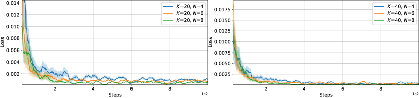
Figure 8: Results of the training curves for potential approximation. Non atomic routing when number of agents $N=4,6,8$, number of nodes $K=20,40$. The y-axis is $\|\Delta\phi-\Delta R_{i}\|^{2}$ (minimising this quantity gives a candidate function for the potential function c.f. Prop. 1).

Appendix F Consensus Optimisation

In what follows, we denote by $\mathcal{C}$ the set of continuously differentiable functions and by $\mathcal{H}$ the set of measurable functions.

To perform the consensus optimisation step, we use the following update processes:

$$\boldsymbol{\rho}^{i}_{l+1}=\sum_{j\in\mathcal{N}}c_{l}(i,j)\rho^{j}_{l}-\alpha\cdot\kappa^{i}_{l}$$ (16)

$$\kappa^{i}_{l+1}=\sum_{j\in\mathcal{N}}c_{l}(i,j)\cdot\kappa^{j}_{l}+\nabla g^{i}(s,\boldsymbol{\rho}^{i}_{l+1})-\nabla g^{i}(s,\boldsymbol{\rho}^{i}_{l})$$ (17)

where $\alpha>0$ is the stepsize and $\boldsymbol{C}_{l}=[c_{l}(i,j)]_{N\times N}$ is the consensus matrix at iteration $l\in\{0,1,\ldots\}$.

Consensus update

0:  Parametric function class $\mathcal{H}$, stepsize $\alpha>0$, initial consensus matrix $\boldsymbol{C}_{0}=[c_{0}(i,j)]_{N\times N}$ , initial parameter $\boldsymbol{\rho}^{i}_{0}\in\mathrm{T},\kappa^{i}_{0}=\nabla g^{i}(s,\boldsymbol{\rho}^{i}_{0})$ for all $i\in\mathcal{N}$.

1:  for $l\in\{0,\ldots,L-1\}$  do

2:     for agent $i\in\mathcal{N}$ do

3:        $\boldsymbol{\rho}^{i}_{l+1}=\sum_{j\in\mathcal{N}}c_{l}(i,j)\rho^{j}_{l}-\alpha\cdot\kappa^{i}_{l}$

4:        $\kappa^{i}_{l+1}=\sum_{j\in\mathcal{N}}c_{l}(i,j)\cdot\kappa^{j}_{l}+\nabla g^{i}(s,\boldsymbol{\rho}^{i}_{l+1})-\nabla g^{i}(s,\boldsymbol{\rho}^{i}_{l})$

5:     end for

6:  end for

7:  Output: The vector of functions $[P_{\rho_{i}}]_{i\in\mathcal{N}}$ for all agent $i\in\mathcal{N}$.

Appendix G Assumptions

Given a pair of metric spaces $\left(X_{1},d_{1}\right)$ and $\left(X_{1},d_{2}\right)$, we say that a function $f:X_{1}\to X_{2}$ is Lipschitz if the constant defined by $L_{f}:=\underset{x_{1}\in X_{1},x_{2}\in X_{2}}{\sup}\frac{d_{2}(f(x_{1}),f(x_{2}))}{d_{1}(x_{1},x_{2})}$ is finite. The constant $L_{f}$ is called the Lipschitz constant. We denote by $L_{R}{{}_{\infty}}:=\max\{L_{R_{1}},\ldots L_{R_{N}}\}$ and similarly for the L-Lipschitz gradients $L_{\frac{\partial R{{}_{\infty}}}{\partial\pi}}:=\max\left\{L_{\frac{\partial R{{}_{1}}}{\partial\pi}},\ldots L_{\frac{\partial R{{}_{N}}}{\partial\pi}}\right\}$.

Given a pair of metric spaces $\left(X_{1},d_{1}\right)$ and $\left(X_{1},d_{2}\right)$, we say that a function $f:X_{1}\to X_{2}$ is Lipschitz if the constant defined by $L_{f}:=\underset{x_{1}\in X_{1},x_{2}\in X_{2}}{\sup}\frac{d_{2}(f(x_{1}),f(x_{2}))}{d_{1}(x_{1},x_{2})}$ is finite. The constant $L_{f}$ is called the Lipschitz constant. We denote by $L_{R}{{}_{\infty}}:=\max\{L_{R_{1}},\ldots L_{R_{N}}\}$ and similarly for the L-Lipschitz gradients $L_{\frac{\partial R{{}_{\infty}}}{\partial\pi}}:=\max\left\{L_{\frac{\partial R{{}_{1}}}{\partial\pi}},\ldots L_{\frac{\partial R{{}_{N}}}{\partial\pi}}\right\}$.

The results of the paper are built under the following assumptions:

Assumption A.2. For any $\theta\in\Theta$, the functions $(R_{i,\theta})_{i\in\mathcal{N}}$ are bounded, measurable functions in the action inputs.
Assumption A.3. The functions $\{R_{i}\}_{i\in\mathcal{N}}$ are Lipschitz and have L-Lipschitz continuous gradients in $\theta\in\Theta$ that is, for any $i\in\mathcal{N}$, there exist constants $L_{R_{i}}>0$ and $L_{\nabla_{\boldsymbol{\theta}}R_{i}}>0$ s.th. for any $s,s^{\prime}\in\mathcal{S}$ and $\forall\boldsymbol{a}\in\boldsymbol{\mathcal{A}},\theta_{a},\theta_{b},\theta_{c},\theta_{d}\in\Theta$ we have that:

$$\left\|\nabla_{\boldsymbol{\theta}}R_{i_{\theta_{a}}}(s^{\prime};s,\boldsymbol{a})-\nabla_{\boldsymbol{\theta}}R_{0_{\theta_{b}}}(s^{\prime};s,\boldsymbol{a})\right\|+\left\|R_{i_{\theta_{c}}}(s^{\prime};s,\boldsymbol{a})-R_{i_{\theta_{d}}}(s^{\prime};s,\boldsymbol{a})\right\|$$

$$\leq L_{\nabla_{\boldsymbol{\theta}}R_{i}}\left\|{\theta_{a}}-{\theta_{b}}\right\|+L_{R_{i}}\left\|{\theta_{c}}-{\theta_{d}}\right\|.$$

Assumption A.4. The functions $\{R_{i}\}_{i\in\mathcal{N}}$ is continuously differentiable in the state and action inputs.
Assumption A.5. The set of policies $\{\pi\}_{i\in\mathcal{N},\boldsymbol{\eta}\in\boldsymbol{E}}$ is differentiable w.r.t. the policy parameter $\boldsymbol{\eta}$.

Assumption A.2. is rudimental and in general required in optimisation and stochastic approximation theory. Assumptions A.3. and A.4. is typical in Q-learning proofs see pg 27 in (Szepesvári & Munos, 2005) (there in fact the transition function is also assumed to be Lipschitz), assumption A7 in (Antos et al., 2008), in (Szepesvári & Munos, 2005) it is assumed that the transition function and reward function are smooth (see pg 21). In this setting, the assumptions are required to construct approximations of $\phi$ in terms of a differential equation. Assumption A.1. is fundamental to the structure of a state-based PG. In particular, it extends the notion of potentiality to the state input. The assumption is used in the proof of Theorem 1. Assumption A.5. is standard and required within the framework of policy gradient and actor-critic methods (Sutton et al., 2000; Silver et al., 2014).

Appendix H Proof of Theoretical Results

H.1 Auxiliary Results

Let us denote by $\left(\mathcal{V},\|\|\right)$ any normed vector space.

Lemma A.

For any $f:\mathcal{V}\times\mathcal{V}\to\mathbb{R},g:\mathcal{V}\times\mathcal{V}\to\mathbb{R}$, we have that:

$$\left\|\underset{a\in\mathcal{V}}{\sup}\>f(a)-\underset{a\in\mathcal{V}}{\sup}\>g(a)\right\|\leq\underset{a\in\mathcal{V}}{\sup}\>\left\|f(a)-g(a)\right\|.$$ (18)

Proof.

$$f(a) \leq\left\|f(a)-g(a)\right\|+g(a)$$ (19)

$$\implies\underset{a\in\mathcal{V}}{\sup}f(a) \leq\underset{a\in\mathcal{V}}{\sup}\{\left\|f(a)-g(a)\right\|+g(a)\}$$

$$\leq\underset{a\in\mathcal{V}}{\sup}\left\|f(a)-g(a)\right\|+\underset{a\in\mathcal{V}}{\sup}\;g(a).$$ (20)

Deducting $\underset{a\in\mathcal{V}}{\sup}\;g(a)$ from both sides of (20) yields:

$$\underset{a\in\mathcal{V}}{\sup}f(a)-\underset{a\in\mathcal{V}}{\sup}g(a)\leq\underset{a\in\mathcal{V}}{\sup}\left\|f(a)-g(a)\right\|.$$ (21)

After reversing the roles of $f$ and $g$ and redoing steps (19) - (20), we deduce the desired result since the RHS of (21) is unchanged. ∎

The proof of the Theorem 1 is established through the following results:

Lemma B.

For any c-SPG, the state transitivity conditions holds whenever the reward functions takes the following form:

$$R_{i}(s,(a^{i},a^{-i}))=g(s,(a^{i},a^{-i}))+k(s)h_{i}(a^{i},a^{-i}),$$

for any functions $g,k,h$ for which $k^{-1}$ exists.

Proof.

To prove the result, we show that the class of games can be rescaled accordingly. Indeed, we first note that $k^{-1}(s)R_{i}(s,(a^{i},a^{-i}))-k^{-1}(s^{\prime})R_{i}(s^{\prime},(a^{i},a^{-i}))=k^{-1}(s)g(s,(a^{i},a^{-i}))-k^{-1}(s^{\prime})g(s^{\prime},(a^{i},a^{-i}))$. Using the invertibility of $k$, we now consider a rescaled game
$\mathcal{M}(s)=\langle\left(\mathcal{A}_{i}\right)_{i\in\mathcal{N}},\left(V_{i}(s)\right)_{i\in\mathcal{N}},\mathcal{N}\rangle$ where $V_{i}:=k^{-1}R_{i}$, then it is easy to see that for these games we have: $V_{i}(s,(a^{i},a^{-i}))-V_{i}(s^{\prime},(a^{i},a^{-i}))=L(s,(a^{i},a^{-i}))-L(s^{\prime},(a^{i},a^{-i}))$ where $L:=k^{-1}g$ and hence the state transitivity assumption is satisfied. ∎

Lemma C.

For any PG, there exists a function $B:\boldsymbol{\Pi}\times\mathcal{S}\to\mathbb{R}$ ($B\in\mathcal{H}$) such that the following holds for any $i\in\mathcal{N},\forall(a^{i}_{t},a^{-i}_{t})\in\boldsymbol{\mathcal{A}},\forall s\in\mathcal{S}$ $R_{i}(s,a^{i}_{t},a^{-i}_{t})=\phi(s,a^{i}_{t},a^{-i}_{t})+F_{i}(s,a^{-i}_{t})$ where $F_{i}$ satisfies $F_{i}(s,a^{-i}_{t})=F_{i}(s^{\prime},a^{-i}_{t})$.

The result generalises dummy-coordination separability known in PGs to a state-based setting (Slade, 1994; Ui, 2000).

Proof of Lemma C.

To establish the forward implication, we make the following observation which is straightforward:

$$R_{i}(s,a^{i}_{t},a^{-i}_{t})-R_{i}(s,a^{\prime i}_{t},a^{-i}_{t})$$

$$=\phi(s,a^{i}_{t},a^{-i}_{t})+F_{i}(s,a^{-i}_{t})-\left(\phi(s,a^{i}_{t},a^{-i}_{t})+F_{i}(s,a^{-i}_{t})\right)$$

$$=\phi(s,a^{i}_{t},a^{-i}_{t})-\phi(s,a^{i}_{t},a^{-i}_{t})$$

To prove the reverse assume that the game is a state-based potential game. Let us now define the function $T_{i}(s,a^{i}_{t},a^{-i}_{t}):=R_{i}(s,a^{i}_{t},a^{-i}_{t})-\phi(s,a^{i}_{t},a^{-i}_{t})$, then we observe that: $R_{i}(s,a^{i}_{t},a^{-i}_{t})-R_{i}(s,a^{\prime i}_{t},a^{-i}_{t})=\phi(s,a^{i}_{t},a^{-i}_{t})-\phi(s,a^{\prime i}_{t},a^{-i}_{t})\iff R_{i}(s,a^{i}_{t},a^{-i}_{t})-\phi(s,a^{i}_{t},a^{-i}_{t})=R_{i}(s,a^{\prime i}_{t},a^{-i}_{t})-\phi(s,a^{\prime i}_{t},a^{-i}_{t})$ and hence $T_{i}(s,a^{i}_{t},a^{-i}_{t})=T_{i}(s,a^{\prime i}_{t},a^{-i}_{t})$ which implies that $T_{i}(s,a^{i}_{t},a^{-i}_{t})\equiv K_{i}(s,a^{-i}_{t})$. In a similar way, writing $T_{i}(s,a^{i}_{t},a^{-i}_{t}):=R_{i}(s,a^{i}_{t},a^{-i}_{t})-\phi(s,a^{i}_{t},a^{-i}_{t})$ and using the state transitive property, we deduce that $T_{i}(s^{\prime},a^{i}_{t},a^{-i}_{t})=T_{i}(s,a^{i}_{t},a^{-i}_{t})$ which settles the proof. ∎

H.2 Proof of Main Results

Proof of Theorem 1

Proposition 4.

There exists a function $B:\boldsymbol{\Pi}\times\mathcal{S}\to\mathbb{R}$ ($B\in\mathcal{H}$) and the following holds for any $i\in\mathcal{N}$

$$\mathbb{E}_{s\sim P(\cdot|)}\left[v^{\boldsymbol{\pi}}_{i}(s)-v^{\boldsymbol{\pi^{\prime}}}_{i}(s)\right]=\mathbb{E}_{s\sim P(\cdot|)}\left[B^{\boldsymbol{\pi}}(s)-B^{\boldsymbol{\pi^{\prime}}}(s)\right].$$ (22)

Proof.

We prove the proposition in two parts beginning with the finite case then extending to the infinite horizon case.

Hence, we first seek to show that for any joint strategy $(\pi_{i},\pi_{-i})\in\boldsymbol{\Pi}$, define by $v_{i,k}$ the value function for the finite horizon game of length $k\in\mathbb{N}$ (i.e.
$v^{\boldsymbol{\pi}}_{i,k}(s):=\mathbb{E}_{s_{t}\sim P,\pi_{i},\pi_{-i}}\left[\sum_{t=0}^{k}\gamma^{t}R_{i}(s_{t},\boldsymbol{a}_{t})|s\equiv s_{0}\right]$ for any $i\in\mathcal{N}$ and $k<\infty$). Then there exists a function $B_{k}:\boldsymbol{\Pi}\times\mathcal{S}\to\mathbb{R}$ such that the following holds for any $i\in\mathcal{N}$ and $\forall\pi_{i},\pi^{\prime}_{i}\in\Pi_{i},\forall\pi_{-i}\in\Pi_{-i}$:

$$\mathbb{E}_{s\sim P(\cdot|)}\left[v^{\boldsymbol{\pi}}_{i,k}(s)-v^{\boldsymbol{\pi^{\prime}}}_{i,k}(s)\right]=\mathbb{E}_{s\sim P(\cdot|)}\left[B_{k}^{\boldsymbol{\pi}}(s)-B_{k}^{\boldsymbol{\pi^{\prime}}}(s)\right].$$ (23)

For the finite horizon case, the result is proven by induction on the number of time steps until the end of the game. Unlike the infinite horizon case, for the finite horizon case the value function and policy have an explicit time dependence.

We consider the case of the proposition at time $T-1$ that is we evaluate the value functions at the penultimate time step. In the following, we employ the shorthands $\boldsymbol{a}_{k}\equiv(a^{i}_{k},a^{-i}_{k})$ and by $\boldsymbol{a^{\prime}}_{k}\equiv(a^{{}^{\prime}i}_{k},a^{-i}_{k})$ for any $k\in\mathbb{N}$ and similarly $\boldsymbol{\pi}(\cdot)\equiv\prod_{j\in\mathcal{N}}\pi_{j}$ and $\boldsymbol{\pi^{\prime}}(\cdot)\equiv\prod_{j\in\mathcal{N}/\{i\}}\pi_{j}(\cdot)\cdot\pi^{\prime}_{i}(\cdot)$. We will also use the shorthands $F^{\boldsymbol{\pi}}\equiv F^{(\pi_{i},\pi_{-i})}$ and $F^{\boldsymbol{\pi^{\prime}}}\equiv F^{(\pi^{\prime}_{i},\pi_{-i})}$ given some function $F$.

In what follows and for the remainder of the script, we employ the following shorthands:

$$\mathcal{P}^{\boldsymbol{a}}_{ss^{\prime}}=:P(s^{\prime};\boldsymbol{a},s),\quad\mathcal{P}^{\boldsymbol{\pi}}_{ss^{\prime}}=:\int_{\boldsymbol{\mathcal{A}}}d\boldsymbol{a}_{t}\boldsymbol{\pi}(\boldsymbol{a}_{t}|s)\mathcal{P}^{\boldsymbol{a}_{t}}_{ss^{\prime}},\quad\mathcal{R}_{i}^{\boldsymbol{\pi}}(s_{t}):=\int_{\boldsymbol{\mathcal{A}}}d\boldsymbol{a}_{t}\boldsymbol{\pi}(\boldsymbol{a}_{t}|s_{t})R_{i}(s_{t},\boldsymbol{a}_{t})$$

$$\boldsymbol{\phi}^{\boldsymbol{\pi}}(s_{t}):=\int_{\boldsymbol{\mathcal{A}}}d\boldsymbol{a}_{t}\boldsymbol{\pi}(\boldsymbol{a}_{t}|s_{t})\phi(s_{t},\boldsymbol{a}_{t}),\quad\boldsymbol{F}_{i}^{\boldsymbol{\pi}}(s_{t}):=\int_{\boldsymbol{\mathcal{A}}}d\boldsymbol{a}_{t}\boldsymbol{\pi}(\boldsymbol{a}_{t}|s_{t})F_{i}(s_{t},\boldsymbol{a}_{t}),\quad\boldsymbol{v}_{i,k}^{\boldsymbol{\pi}}(s_{t}):=\int_{\boldsymbol{\mathcal{A}}}d\boldsymbol{a}_{t}\boldsymbol{\pi}(\boldsymbol{a}_{t}|s_{t})v^{\boldsymbol{\pi}}_{i,k}(s_{t},\boldsymbol{a}_{t})$$

In this case, we have that:

$$\mathbb{E}_{s_{T-1}\sim P(\cdot|)}\left[v^{\boldsymbol{\pi}}_{i,T-1}(s_{T-1})-v^{\boldsymbol{\pi^{\prime}}}_{i,T-1}(s_{T-1})\right]$$

$$=\mathbb{E}_{s_{T-1}\sim P(\cdot|)}\left[\mathcal{R}_{i}^{\boldsymbol{\pi}}(s_{T})+\gamma\int_{\mathcal{S}}ds_{T}\int_{\boldsymbol{\mathcal{A}}}\mathcal{P}^{\boldsymbol{\pi}}_{s_{T}s_{T-1}}v_{i}^{\boldsymbol{\pi}}(s_{T})-\left(\mathcal{R}_{i}^{\boldsymbol{\pi^{\prime}}}(s_{T})+\gamma\int_{\mathcal{S}}ds_{T}\mathcal{P}^{\boldsymbol{\pi^{\prime}}}_{s_{T}s_{T-1}}v_{i}^{\boldsymbol{\pi^{\prime}}}(s_{T})\right)\right]$$

$$=\mathbb{E}_{s_{T-1}\sim P(\cdot|)}\Bigg{[}\boldsymbol{\phi}^{\boldsymbol{\pi}}(s_{T})-\boldsymbol{\phi}^{\boldsymbol{\pi^{\prime}}}(s_{T})+\gamma\int_{\mathcal{S}}ds_{T}\mathcal{P}^{\boldsymbol{\pi}}_{s_{T}s_{T-1}}v_{i}^{\boldsymbol{\pi}}(s_{T})-\gamma\int_{\mathcal{S}}ds\mathcal{P}^{\boldsymbol{\pi^{\prime}}}_{s_{T}s_{T-1}}v_{i}^{\boldsymbol{\pi^{\prime}}}(s_{T})\Bigg{]}$$

$$\begin{aligned} =\mathbb{E}_{s_{T-1}\sim P(\cdot|)}\Bigg{[}&\boldsymbol{\phi}^{\boldsymbol{\pi}}(s_{T-1})-\boldsymbol{\phi}^{\boldsymbol{\pi^{\prime}}}(s_{T-1})+\gamma\mathbb{E}_{s_{T}\sim P(\cdot|)}\Bigg{[}\boldsymbol{v}_{i}^{\boldsymbol{\pi}}(s_{T})-\boldsymbol{v}_{i}^{\boldsymbol{\pi^{\prime}}}(s_{T})\Bigg{]}\Bigg{]}.\end{aligned}$$

We now observe that for any $\pi_{i}\in\Pi_{i}$ and for any $\pi_{-i}\in\Pi_{-i}$ we have that $\forall i\in\mathcal{N},\;v_{i}^{\pi^{i},\pi^{-i}}(s_{T})=\mathbb{E}_{s_{T}\sim P(\cdot|)}\left[\mathcal{R}_{i}^{\boldsymbol{\pi}}(s_{T})\right]$, moreover we have that for any $\pi_{i},\pi_{i}^{\prime}\in\Pi_{i}$ and for any $i\in\mathcal{N}$, we have

$$\mathbb{E}_{s_{T}\sim P(\cdot|)}\Bigg{[}\mathcal{R}_{i}^{\boldsymbol{\pi}}(s_{T})-\mathcal{R}_{i}^{\boldsymbol{\pi^{\prime}}}(s_{T})\Bigg{]}$$

$$=\int_{\mathcal{S}}ds_{T}\mathcal{P}^{\boldsymbol{\pi}}_{s_{T}s_{T-1}}\mathcal{R}_{i}^{\boldsymbol{\pi}}(s_{T})-\int_{\mathcal{S}}ds_{T}\mathcal{P}^{\boldsymbol{\pi^{\prime}}}_{s_{T}s_{T-1}}\mathcal{R}_{i}^{\boldsymbol{\pi^{\prime}}}(s_{T})$$

$$=\int_{\mathcal{S}}ds_{T}\mathcal{P}^{\boldsymbol{\pi}}_{s_{T}s_{T-1}}\left[\boldsymbol{\phi}^{\boldsymbol{\pi}}(s_{T})+\boldsymbol{F}_{i}(a^{-i}_{T})\right]-\int_{\mathcal{S}}ds_{T}\mathcal{P}^{\boldsymbol{\pi^{\prime}}}_{s_{T}s_{T-1}}\left[\boldsymbol{\phi}^{\boldsymbol{\pi^{\prime}}}(s_{T})+\boldsymbol{F}_{i}(a^{-i}_{T})\right]$$

$$=\int_{\mathcal{S}}ds_{T}\mathcal{P}^{\boldsymbol{\pi}}_{s_{T}s_{T-1}}\boldsymbol{\phi}^{\boldsymbol{\pi}}(s_{T})-\int_{\mathcal{S}}ds_{T}\mathcal{P}^{\boldsymbol{\pi^{\prime}}}_{s_{T}s_{T-1}}\boldsymbol{\phi}^{\boldsymbol{\pi^{\prime}}}(s_{T})+\int_{\mathcal{S}}ds_{T}\mathcal{P}^{\boldsymbol{\pi}}_{s_{T}s_{T-1}}\boldsymbol{F}_{i}(a^{-i}_{T})-\int_{\mathcal{S}}ds_{T}\mathcal{P}^{\boldsymbol{\pi^{\prime}}}_{s_{T}s_{T-1}}\boldsymbol{F}_{i}(a^{-i}_{T})$$

$$=\int_{\mathcal{S}}ds_{T}\mathcal{P}^{\boldsymbol{\pi}}_{s_{T}s_{T-1}}\boldsymbol{\phi}^{\boldsymbol{\pi}}(s_{T})-\int_{\mathcal{S}}ds_{T}\mathcal{P}^{\boldsymbol{\pi^{\prime}}}_{s_{T}s_{T-1}}\boldsymbol{\phi}^{\boldsymbol{\pi^{\prime}}}(s_{T})$$

$$=\mathbb{E}_{s_{T}\sim P(\cdot|)}\left[\boldsymbol{\phi}^{\boldsymbol{\pi}}(s_{T})-\boldsymbol{\phi}^{\boldsymbol{\pi^{\prime}}}(s_{T})\right]$$

Since

$$\int_{\mathcal{S}}ds_{T}\mathcal{P}^{\boldsymbol{\pi}}_{s_{T}s_{T-1}}\boldsymbol{F}_{i}(a^{-i}_{T})-\int_{\mathcal{S}}ds_{T}\mathcal{P}^{\boldsymbol{\pi^{\prime}}}_{s_{T}s_{T-1}}\boldsymbol{F}_{i}(a^{-i}_{T})$$

$$=\int_{\mathcal{A}_{-i}}\pi_{i}(da^{i},s_{T-1})F_{i}(a^{-i})\int_{\mathcal{A}_{i}}\pi_{-i}(da^{-i},s_{T-1})\int_{\mathcal{S}}ds_{T}P(s_{T};s_{T-1},\boldsymbol{a}_{T})$$

$$\qquad\qquad\qquad-\int_{\mathcal{A}_{-i}}\pi^{\prime}_{i}(da^{\prime i},s_{T-1})F_{i}(a^{-i})\int_{\mathcal{A}_{i}}\pi_{-i}(da^{-i},s_{T-1})\int_{\mathcal{S}}ds_{T}P(s_{T};s_{T-1},\boldsymbol{a^{\prime}}_{T})$$

$$=\int_{\mathcal{A}_{-i}}\pi_{-i}(da^{-i},s_{T-1})F_{i}(a^{-i})\left\{\int_{\mathcal{A}_{i}}\pi_{i}(da^{i},s_{T-1})-\int_{\mathcal{A}_{i}}\pi^{\prime}_{i}(da^{\prime i},s_{T-1})\right\}$$

$$=0$$

Hence, we find that

$$\mathbb{E}_{s_{T-1}\sim P(\cdot|)}\left[v^{\boldsymbol{\pi}}_{i,T-1}(s_{T-1})-v^{\boldsymbol{\pi^{\prime}}}_{i,T-1}(s_{T-1})\right]$$

$$=\mathbb{E}_{s_{T-1}\sim P(\cdot|)}\left[\boldsymbol{\phi}^{\boldsymbol{\pi}}(s_{T-1})-\boldsymbol{\phi}^{\boldsymbol{\pi^{\prime}}}(s_{T-1})+\gamma\int_{\mathcal{S}}ds_{T}\mathcal{P}^{\boldsymbol{\pi}}_{s_{T}s_{T-1}}\boldsymbol{\phi}^{\boldsymbol{\pi}}(s_{T})-\gamma\int_{\mathcal{S}}ds_{T}\mathcal{P}^{\boldsymbol{\pi^{\prime}}}_{s_{T}s_{T-1}}\boldsymbol{\phi}^{\boldsymbol{\pi^{\prime}}}(s_{T})\right]$$

$$=\mathbb{E}_{s_{T-1}\sim P(\cdot|)}\left[\boldsymbol{\phi}^{\boldsymbol{\pi}}(s_{T-1})-\boldsymbol{\phi}^{\boldsymbol{\pi^{\prime}}}(s_{T})+\gamma\mathbb{E}_{s_{T}\sim P(s_{T}|\cdot)}\left[\boldsymbol{\phi}^{\boldsymbol{\pi}}(s_{T-1})-\boldsymbol{\phi}^{\boldsymbol{\pi^{\prime}}}(s_{T})\right]\right]$$

$$=\mathbb{E}_{s_{T-1}\sim P(\cdot|)}\Bigg{[}B_{T-1}^{\boldsymbol{\pi}}(s_{T-1})-B_{T-1}^{\boldsymbol{\pi^{\prime}}}(s_{T-1})\Bigg{]},$$

using the iterated law of expectations in the last line and where

$$B^{\boldsymbol{\pi}}_{T}(s):=\mathbb{E}_{s_{t}\sim P,\pi_{i},\pi_{-i}}\left[\sum_{t=0}^{T}\gamma^{t}\phi(s_{t},\boldsymbol{a}_{t})|s\equiv s_{0}]\right].$$ (24)

Hence, we have succeeded in proving that the expression (22) holds for $T-k$ when $k=1$.

Our next goal is to prove that the expression holds for any $0<k\leq T$.

Note that for any $T\geq k>0$, we can write (24) as

$$B^{\boldsymbol{\pi}}_{T-k}(s)=\mathbb{E}_{\pi_{i},\pi_{-i}}\left[\phi(s,\boldsymbol{a}_{k})+\gamma\int_{\mathcal{S}}ds^{\prime}P(s^{\prime};s,\boldsymbol{a}_{k})B_{T-(k+1)}^{\pi^{i},\pi^{-i}}(s^{\prime})\cdot 1_{k\leq T}\right].$$

Now we consider the case when we evaluate the expression (22) for any $0<k\leq T$. Our inductive hypothesis is the expression holds for some $0<k\leq T$, that is for a $0<k\leq T$ we have that:

$$\mathbb{E}_{s_{T-k}\sim P(\cdot|)}\left[v^{\boldsymbol{\pi}}_{i,k}(s_{T-k})-v^{\boldsymbol{\pi^{\prime}}}_{i,k}(s_{T-k})\right]=\mathbb{E}_{s_{T-k}\sim P(\cdot|)}\left[B^{\boldsymbol{\pi}}_{k}(s_{T-k})-B^{\boldsymbol{\pi^{\prime}}}_{k}(s_{T-k})\right].$$ (25)

It is easy to see that given (25) and Lemma C, it must be the case that:

$$\mathbb{E}_{s_{T-k}\sim P(\cdot|)}\left[v^{\boldsymbol{\pi}}_{i,k}(s_{T-k})\right]=\mathbb{E}_{s_{T-k}\sim P(\cdot|)}\left[B^{\boldsymbol{\pi}}_{k}(s_{T-k})+G^{\pi_{-i}}_{i,k}(s_{T-k})\right].$$ (26)

where $G^{\pi_{-i}}_{i,k}(s):=\mathbb{E}_{P,\pi_{-i}}\left[\sum_{t=0}^{k}\gamma^{t}F_{-i}(s,a_{t}^{-i})\right]$.

Moreover, we recall that $F_{-i}$ satisfies the condition $F_{-i}(s,a^{-i}_{t})=F_{-i}(s^{\prime},a^{-i}_{t})$, hence $G^{\pi_{-i}}_{i,k}(s)=G^{\pi_{-i}}_{i,k}(s^{\prime})$ so from now on we drop the dependence on $s$ and write $G^{\pi_{-i}}_{i,k}$.

It remains to show that the expression holds for $k+1$ time steps prior to the end of the horizon. The result can be obtained using the dynamic programming principle and the base case ($k=1$) result, indeed we have that

$$\mathbb{E}_{s_{T-(k+1)}\sim P(\cdot|)}\left[v^{\boldsymbol{\pi}}_{i,k+1}(s_{T-(k+1)})-v^{\boldsymbol{\pi^{\prime}}}_{i,k+1}(s_{T-(k+1)})\right]$$

$$\begin{aligned} =\mathbb{E}_{s_{T-(k+1)}\sim P(\cdot|)}\Bigg{[}\mathcal{R}_{i}^{\boldsymbol{\pi}}(s_{T-(k+1)})&+\gamma\int_{\mathcal{S}}ds_{T-k}\mathcal{P}^{\boldsymbol{\pi}}_{s_{T-(k+1)}s_{T-k}}\boldsymbol{v}_{i,k}^{\boldsymbol{\pi}}(s_{T-k})\\ &-\mathcal{R}_{i}^{\boldsymbol{\pi^{\prime}}}(s_{T-(k+1)})-\gamma\int_{\mathcal{S}}ds_{T-k}\mathcal{P}^{\boldsymbol{\pi^{\prime}}}_{s_{T-(k+1)}s_{T-k}}\boldsymbol{v}_{i,k}^{\boldsymbol{\pi^{\prime}}}(s_{T-k})\Bigg{]}\end{aligned}$$

$$=\mathbb{E}_{s_{T-(k+1)}\sim P(\cdot|)}\left[\mathcal{R}_{i}^{\boldsymbol{\pi}}(s_{T-(k+1)})-\mathcal{R}_{i}^{\boldsymbol{\pi^{\prime}}}(s_{T-(k+1)})\right]$$

$$+\gamma\mathbb{E}_{s_{T-(k+1)}\sim P(\cdot|)}\Bigg{[}\int_{\mathcal{S}}ds\mathcal{P}^{\boldsymbol{\pi}}_{s_{T-(k+1)}s_{T-k}}\boldsymbol{v}_{i,k}^{\boldsymbol{\pi}}(s_{T-k})-\mathcal{P}^{\boldsymbol{\pi^{\prime}}}_{s_{T-(k+1)}s_{T-k}}\boldsymbol{v}_{i,k}^{\boldsymbol{\pi^{\prime}}}(s_{T-k})\Bigg{]}.$$

Studying the terms under the first expression, we observe that by construction, we have that:

$$\mathbb{E}_{s_{T-(k+1)}\sim P(\cdot|)}\Bigg{[}\mathcal{R}_{i}^{\boldsymbol{\pi}}(s_{T-(k+1)})-\mathcal{R}_{i}^{\boldsymbol{\pi^{\prime}}}(s_{T-(k+1)})\Bigg{]}=\mathbb{E}_{s_{T-(k+1)}\sim P(\cdot|)}\left[\boldsymbol{\phi}^{\boldsymbol{\pi}}(s_{T-(k+1)})-\boldsymbol{\phi}^{\boldsymbol{\pi}^{\prime}}(s_{T-(k+1)})\right].$$ (27)

We now study the terms within the second expectation.

Using (25) (i.e. the inductive hypothesis), we find that:

$$\int_{\mathcal{S}}ds_{T-k}\mathcal{P}^{\boldsymbol{\pi}}_{s_{T-k}s_{T-k-1}}\boldsymbol{v}_{i,k}^{\boldsymbol{\pi}}(s_{T-k})-\int_{\mathcal{S}}ds_{T-k}\mathcal{P}^{\boldsymbol{\pi^{\prime}}}_{s_{T-k}s_{T-k-1}}\boldsymbol{v}_{i,k}^{\boldsymbol{\pi^{\prime}}}(s_{T-k})$$

$$=\int_{\mathcal{S}}ds_{T-k}\mathcal{P}^{\boldsymbol{\pi}}_{s_{T-k}s_{T-k-1}}\left[\boldsymbol{B}_{k}^{\boldsymbol{\pi}}(s_{T-k})+\boldsymbol{G}_{i,k}^{\pi_{-i}}\right]-\int_{\mathcal{S}}ds_{T-k}\mathcal{P}^{\boldsymbol{\pi^{\prime}}}_{s_{T-k}s_{T-k-1}}\left[\boldsymbol{B}_{k}^{\boldsymbol{\pi^{\prime}}}(s_{T-k})+\boldsymbol{G}_{i,k}^{\pi_{-i}}\right]$$

$$\begin{aligned} =\int_{\mathcal{S}}ds_{T-k}\mathcal{P}^{\boldsymbol{\pi}}_{s_{T-k}s_{T-k-1}}\boldsymbol{B}_{k}^{\boldsymbol{\pi}}(s_{T-k})&-\int_{\mathcal{S}}ds_{T-k}\mathcal{P}^{\boldsymbol{\pi^{\prime}}}_{s_{T-k}s_{T-k-1}}\boldsymbol{B}_{k}^{\boldsymbol{\pi^{\prime}}}(s_{T-k})\\ &+\int_{\mathcal{S}}ds_{T-k}\mathcal{P}^{\boldsymbol{\pi}}_{s_{T-k}s_{T-k-1}}\boldsymbol{G}_{i,k}^{\pi_{-i}}-\int_{\mathcal{S}}ds_{T-k}\mathcal{P}^{\boldsymbol{\pi^{\prime}}}_{s_{T-k}s_{T-k-1}}\boldsymbol{G}_{i,k}^{\pi_{-i}}\end{aligned}$$

We now observe that

$$\int_{\mathcal{S}}ds_{T-k}\mathcal{P}^{\boldsymbol{\pi}}_{s_{T-k}s_{T-k-1}}\boldsymbol{G}_{i,k}^{\pi_{-i}}-\int_{\mathcal{S}}ds_{T-k}\mathcal{P}^{\boldsymbol{\pi^{\prime}}}_{s_{T-k}s_{T-k-1}}\boldsymbol{G}_{i,k}^{\pi_{-i}}$$

$$=\int_{\mathcal{S}}ds_{T-k}\int_{\boldsymbol{\mathcal{A}}}\Bigg{[}\pi_{i}(da^{i}_{T-(k+1)},s_{T-(k+1)})-\pi^{\prime}_{i}(da^{i}_{T-(k+1)},s_{T-(k+1)})\Bigg{]}$$

$$\qquad\qquad\qquad\cdot P(s_{T-k};s_{T-(k+1)},\boldsymbol{a}_{T-(k+1)})\pi_{-i}(da^{-i}_{T-(k+1)},s_{T-(k+1)})G^{\pi_{-i}}_{i,k}$$

$$=\int_{\mathcal{S}}ds_{T-k}\int_{\mathcal{A}_{-i}}\pi_{-i}(da^{-i}_{T-(k+1)},s_{T-(k+1)})$$

$$\qquad\qquad\qquad\qquad\cdot\left(P(s_{T-k};s_{T-(k+1)},\pi_{i},a^{-i}_{T-(k+1)})-P(s_{T-k};s_{T-(k+1)},\pi^{\prime}_{i},a^{-i}_{T-(k+1)})\right)G^{\pi_{-i}}_{i,k}$$

$$=0$$

We now find that:

$$\int_{\mathcal{S}}ds_{T-k}\mathcal{P}^{\boldsymbol{\pi}}_{s_{T-k}s_{T-k-1}}\boldsymbol{v}_{i,k}^{\boldsymbol{\pi}}(s_{T-k})-\int_{\mathcal{S}}ds_{T-k}\mathcal{P}^{\boldsymbol{\pi^{\prime}}}_{s_{T-k}s_{T-k-1}}\boldsymbol{v}_{i,k}^{\boldsymbol{\pi^{\prime}}}(s_{T-k})$$

$$=\int_{\mathcal{S}}ds_{T-k}\mathcal{P}^{\boldsymbol{\pi}}_{s_{T-k}s_{T-k-1}}\boldsymbol{B}_{k}^{\boldsymbol{\pi}}(s_{T-k})-\int_{\mathcal{S}}ds_{T-k}\mathcal{P}^{\boldsymbol{\pi^{\prime}}}_{s_{T-k}s_{T-k-1}}\boldsymbol{B}_{k}^{\boldsymbol{\pi^{\prime}}}(s_{T-k})$$ (28)

Now combining (27) and (28) leads to the fact that:

$$\mathbb{E}_{s_{T-(k+1)}\sim P(\cdot|)}\left[v^{\boldsymbol{\pi}}_{i,k+1}(s_{T-(k+1)})-v^{\boldsymbol{\pi^{\prime}}}_{i,k+1}(s_{T-(k+1)})\right]$$

$$\begin{aligned} =\mathbb{E}_{s_{T-(k+1)}\sim P(\cdot|)}\Bigg{[}\int_{\mathcal{S}}ds_{T-k}\mathcal{P}^{\boldsymbol{\pi}}_{s_{T-k}s_{T-k-1}}\boldsymbol{B}_{k}^{\boldsymbol{\pi}}(s_{T-k})&-\int_{\mathcal{S}}ds_{T-k}\mathcal{P}^{\boldsymbol{\pi^{\prime}}}_{s_{T-k}s_{T-k-1}}\boldsymbol{B}_{k}^{\boldsymbol{\pi^{\prime}}}(s_{T-k})\Bigg{]}\\ &+\mathbb{E}_{s_{T-(k+1)}\sim P(\cdot|)}\left[\boldsymbol{\phi}^{\boldsymbol{\pi}}(s_{T-(k+1)})-\boldsymbol{\phi}^{\boldsymbol{\pi}^{\prime}}(s_{T-(k+1)})\right]\end{aligned},$$

from which we immediately deduce that

$$\mathbb{E}_{s_{T-(k+1)}\sim P(\cdot|)}\left[v^{\boldsymbol{\pi}}_{i,k+1}(s_{T-(k+1)})-v^{\boldsymbol{\pi^{\prime}}}_{i,k+1}(s_{T-(k+1)})\right]=\mathbb{E}_{s_{T-(k+1)}\sim P(\cdot|)}\left[B^{\boldsymbol{\pi}}_{k+1}(s_{T-(k+1)})-B^{\boldsymbol{\pi^{\prime}}}_{k+1}(s_{T-(k+1)})\right],$$

where

$$B^{\boldsymbol{\pi}}_{k}(s)=\mathbb{E}_{\pi_{i},\pi_{-i}}\left[\phi(s_{k},\boldsymbol{a}_{k})+\gamma\int_{\mathcal{S}}ds^{\prime}P(s^{\prime};s,\boldsymbol{a}_{k})B_{k-1}^{\pi^{i},\pi^{-i}}(s^{\prime})\right],$$

from which we deduce the result. ∎

Thus far we have established the relation (23) holds only for the finite horizon case. We now extend the coverage to the infinite horizon case in which we can recover the use of stationary strategies. Before doing so, we require the following results:

Lemma D.

For any $t^{\prime}<\infty$, define by $B^{\boldsymbol{\pi}}_{t^{\prime}}:\mathbb{N}\times\Pi_{i}\times\Pi_{-i}\times\mathcal{S}\to\mathbb{R}$ the following function:

$$B^{\boldsymbol{\pi}}_{t^{\prime}}(s):=\mathbb{E}_{s_{t}\sim P,\pi_{i},\pi_{-i}}\left[\sum_{t=0}^{T}\gamma^{t}\phi(s_{t},\boldsymbol{a}_{t})|s\equiv s_{0}\right].$$

then $\exists B^{\boldsymbol{\pi}}:\Pi_{i}\times\Pi_{-i}\times\mathcal{S}\to\mathbb{R}$ s.t. $\forall s\in\mathcal{S}$ and for any $\pi_{i}\in\Pi_{i},\pi_{-i}\in\Pi_{-i}$,

$$\underset{t\to\infty}{\lim}B^{\boldsymbol{\pi}}_{t}(s)=B^{\boldsymbol{\pi}}(s),$$

where for any $\pi_{i}\in\Pi_{i},\pi_{-i}\in\Pi_{-i}$, the function $B^{\boldsymbol{\pi}}$ is given by:
$B^{\boldsymbol{\pi}}(s):=\mathbb{E}_{s_{t}\sim P,\pi_{i},\pi_{-i}}\left[\sum_{t=0}^{\infty}\gamma^{t}\phi(s_{t},\boldsymbol{a}_{t})|s\equiv s_{0}\right]$.

Proof.

We prove the result by showing that the sequence $B^{\boldsymbol{\pi}}_{n},B^{\boldsymbol{\pi}}_{n+1},\ldots$ converges uniformly, that is the sequence is a Cauchy sequence. In particular, we show that $\forall\epsilon>0$, $\exists T^{\prime}>0$ s.th. $\forall t^{\prime},t^{\prime\prime}>T^{\prime}$ and for any $\pi_{i}\in\Pi_{i},\pi_{-i}\in\Pi_{-i}$

$$\left\|B^{\boldsymbol{\pi}}_{t^{\prime}}-B^{\boldsymbol{\pi}}_{t^{\prime\prime}}\right\|<\epsilon.$$

Firstly, we deduce that the function $\phi$ is bounded since each $R_{i}$ is bounded also (c.f. (43)). Now w.log., consider the case when $t^{\prime}\geq t^{\prime\prime}$. We begin by observing the fact that

$$B^{\boldsymbol{\pi}}_{t^{\prime}}(s)-B^{\boldsymbol{\pi}}_{t^{\prime\prime}}(s)$$

$$=\mathbb{E}_{s_{t}\sim P(\cdot;s_{t-1},a_{t-1}),\pi_{i},\pi_{-i}}\left[\sum_{t=0}^{t^{\prime}}\gamma^{t}\phi_{t}(s_{t},\boldsymbol{a}_{t})-\sum_{t=0}^{t^{\prime\prime}}\gamma^{t}\phi_{t}(s_{t},\boldsymbol{a}_{t})\right]$$

$$=\mathbb{E}_{s_{t}\sim P(\cdot;s_{t-1},a_{t-1}),\pi_{i},\pi_{-i}}\left[\sum_{t=t^{\prime\prime}}^{t^{\prime}}\gamma^{t}\phi_{t}(s_{t},\boldsymbol{a}_{t})\right].$$

Hence, we find that

$$\;\left|B^{\boldsymbol{\pi}}_{t^{\prime}}(s)-B^{\boldsymbol{\pi}}_{t^{\prime\prime}}(s)\right|$$

$$=\left|\mathbb{E}_{s_{t}\sim P(\cdot;s_{t-1},a_{t-1}),\pi_{i},\pi_{-i}}\left[\sum_{t=t^{\prime\prime}}^{t^{\prime}}\gamma^{t}\phi_{t}(s_{t},\boldsymbol{a}_{t})\right]\right|$$

$$\leq\sum_{t=t^{\prime\prime}}^{t^{\prime}}\gamma^{t}\|\phi\|_{\infty}\leq|\gamma|\frac{\left|\gamma^{t^{\prime\prime}}-\gamma^{t^{\prime}}\right|}{1-\gamma}\|\phi\|_{\infty}$$

$$\leq|\gamma^{t^{\prime\prime}}|\frac{\left|1-\gamma^{t^{\prime}-t^{\prime\prime}}\right|}{1-\gamma}\|\phi\|_{\infty}$$

$$\leq\frac{|\gamma^{t^{\prime\prime}}|}{1-\gamma}\|\phi\|_{\infty}=e^{t^{\prime\prime}\ln\gamma}\frac{\|\phi\|_{\infty}}{1-\gamma}$$

$$=e^{-t^{\prime\prime}|\ln\gamma|}\left(\frac{\|\phi\|_{\infty}}{1-\gamma}\right)\leq e^{-T^{\prime}|\ln\gamma|}\left(\frac{\|\phi\|_{\infty}}{1-\gamma}\right),$$

using Cauchy-Schwarz and since $t^{\prime}\geq t^{\prime\prime}>T^{\prime}$ and $\gamma\in[0,1[$. The inequality of the proposition is true whenever $T^{\prime}$ is chosen to satisfy

$$T^{\prime}\geq\left|\ln{(\epsilon)}(\ln{(\gamma)}\left(\frac{\|\phi\|_{\infty}}{1-\gamma}\right)^{-1}\right|,$$

hence the result is proven. ∎

We are now in a position to extend the dynamic potential property (23) to the infinite horizon case:

Proof.

The result is proven by contradiction.

To this end, let us firstly assume there exists a constant $c\neq 0$ s.th.

$$\mathbb{E}_{s\sim P(\cdot|)}\left[v^{\boldsymbol{\pi}}_{i}(s)-v^{\boldsymbol{\pi^{\prime}}}_{i}(s)\right]-\mathbb{E}_{s\sim P(\cdot|)}\left[B^{\boldsymbol{\pi}}_{i}(s)-B^{\boldsymbol{\pi^{\prime}}}_{i}(s)\right]=c.$$

Let us now define the following quantities for any $s\in\mathcal{S}$ and for each $\pi_{i}\in\Pi_{i}$ and $\pi_{-i}\in\Pi_{-i}$ and $\forall\theta\in\Theta,\forall i\in\mathcal{N}$:

$$v_{i,T^{\prime}}^{\boldsymbol{\pi}}(s):=\sum_{t=1}^{T^{\prime}}\int_{\mathcal{S}}ds_{j+1}\mu(s_{0})\pi_{i}(a^{i}_{0},s_{0})\pi_{-i}(a^{-i}_{0},s_{0})\prod_{j=1}^{t-1}\gamma^{j}P(s_{j+1}|s_{j},a^{i}_{j},a^{-i}_{j})$$

$$\cdot\pi_{i}(a^{i}_{j}|s_{j})\pi_{-i}(a^{-i}_{j}|s_{j})R_{i}(s_{j},a^{i}_{j},a^{-i}_{j})$$ ,

and

$$B_{T^{\prime}}^{\boldsymbol{\pi}}(s)$$

$$\begin{aligned} :=\sum_{t=1}^{T^{\prime}}\int_{\mathcal{S}}ds_{j+1}\mu(s_{0})\pi_{i}(a^{i}_{0},s_{0})\pi_{-i}(a^{-i}_{0},s_{0})\prod_{j=1}^{t-1}\gamma^{j}P(s_{j+1}|s_{j},a^{i}_{j},a^{-i}_{j})\pi_{i}(a^{i}_{j}|s_{j})\pi_{-i}(a^{-i}_{j}|s_{j})&\\ \cdot\phi(s_{j},a^{i}_{j},a^{-i}_{j})&,\end{aligned}$$

so that the quantity $v_{i,T^{\prime}}^{\boldsymbol{\pi}}(s)$ measures the expected cumulative return until the point $T^{\prime}<\infty$.

Hence, we straightforwardly deduce that

$$v_{i}^{\boldsymbol{\pi}}(s)\equiv v_{i,\infty}^{\boldsymbol{\pi}}(s)$$

$$\begin{aligned} =v_{i,T^{\prime}}^{\boldsymbol{\pi}}(s)+\gamma^{T^{\prime}}\int_{\mathcal{S}}ds_{j+1}\mu(s_{0})\pi_{i}(a^{i}_{0},s_{0})\pi_{-i}(a^{-i}_{0},s_{0})\prod_{j=1}^{T^{\prime}}P(s_{j+1}|s_{j},a^{i}_{j},a^{-i}_{j})\pi_{i}(a^{i}_{j}|s_{j})&\\ \cdot\pi_{-i}(a^{-i}_{j}|s_{j})v_{i}^{\boldsymbol{\pi}}(s_{T^{\prime}}).&\end{aligned}$$

Our first task is to establish that the quantity $\left|\underset{t\to\infty}{\lim}\mathbb{E}_{s\sim P(\cdot|)}\left[B^{\boldsymbol{\pi}}_{i,t}(s)-B^{\boldsymbol{\pi^{\prime}}}_{i,t}(s)\right]\right|$ is in fact, well-defined for any $s\in\mathcal{S}$ and $\forall i\in\mathcal{N}$.

This is true since by (25) for any $t>0$ we have that

$$\left|\mathbb{E}_{s\sim P(\cdot|)}\left[B^{\boldsymbol{\pi}}_{i,t}(s)-B^{\boldsymbol{\pi^{\prime}}}_{i,t}(s)\right]\right|=\left|\mathbb{E}_{s\sim P(\cdot|)}\left[v^{\boldsymbol{\pi}}_{i,t}(s)-v^{\boldsymbol{\pi^{\prime}}}_{i,t}(s)\right]\right|,$$ (29)

and hence we have that

$$\left|\mathbb{E}_{s\sim P(\cdot|)}\left[B^{\boldsymbol{\pi}}(s)-B^{\boldsymbol{\pi^{\prime}}}(s)\right]\right|<\infty.$$

To see this, we firstly observe that by the boundedness of $R_{i}$, $\exists c>0$ s.th. $\forall t\in\mathbb{N},\forall i\in\mathcal{N}$ and for any $\pi_{i}\in\Pi_{i},\pi_{-i}\in\Pi_{-i}$

$$\left|v^{\boldsymbol{\pi}}_{i,t}(s)-v^{\boldsymbol{\pi^{\prime}}}_{i,t}(s)\right|<c.$$

This is true since for any $k<\infty$ we have

$$\qquad\qquad\qquad\qquad v_{i,k}^{\boldsymbol{\pi}}(s)-v_{i,k}^{\boldsymbol{\pi^{\prime}}}(s)$$

$$=\mathbb{E}_{s_{t}\sim P,\pi_{i},\pi_{-i}}\left[\sum_{t=0}^{k}\gamma^{t}R_{i}(s_{t},\boldsymbol{a}_{t})\right]-\mathbb{E}_{s_{t}\sim P,\pi^{\prime}_{i},\pi_{-i}}\left[\sum_{t=0}^{k}\gamma^{t}R_{i}(s_{t},\boldsymbol{a}_{t})\right]$$

$$\leq\left|\mathbb{E}_{s_{t}\sim P,\pi_{i},\pi_{-i}}\left[\sum_{t=0}^{k}\gamma^{t}R_{i}(s_{t},\boldsymbol{a}_{t})\right]-\mathbb{E}_{s_{t}\sim P,\pi^{\prime}_{i},\pi_{-i}}\left[\sum_{t=0}^{k}\gamma^{t}R_{i}(s_{t},\boldsymbol{a}_{t})\right]\right|$$

$$\leq 2\sum_{t=0}^{k}\gamma^{t}\|R_{i}\|_{\infty}=2\frac{1-\gamma^{k}}{1-\gamma}\|R_{i}\|_{\infty}.$$

Therefore, by the bounded convergence theorem we have that

$$\underset{t\to\infty}{\lim}\left|\mathbb{E}_{s\sim P(\cdot|)}\left[v^{\boldsymbol{\pi}}_{i,t}(s)-v^{\boldsymbol{\pi^{\prime}}}_{i,t}(s)\right]\right|<\infty.$$ (30)

Now, using (29), we deduce that for any $\epsilon>0$, the following statement holds:

$$\left|\mathbb{E}_{s\sim P(\cdot|)}\left[B^{\boldsymbol{\pi}}_{i,t}(s)-B^{\boldsymbol{\pi^{\prime}}}_{i,t}(s)\right]\right|<\left|\mathbb{E}_{s\sim P(\cdot|)}\left[v^{\boldsymbol{\pi}}_{i,t}(s)-v^{\boldsymbol{\pi^{\prime}}}_{i,t}(s)\right]\right|+\epsilon,$$

which after taking the limit as $t\to\infty$ and using (30), Lemma D and the dominated convergence theorem, we find that

$$\underset{t\to\infty}{\lim}\left|\mathbb{E}_{s\sim P(\cdot|)}\left[B^{\boldsymbol{\pi}}_{i,t}(s)-B^{\boldsymbol{\pi^{\prime}}}_{i,t}(s)\right]\right|<\infty.$$

Next we observe that:

$$c =\mathbb{E}_{s\sim P(\cdot|)}\left[\left(v_{i}^{\boldsymbol{\pi}}-v_{i}^{\boldsymbol{\pi^{\prime}}}\right)(s)\right]-\mathbb{E}_{s\sim P(\cdot|)}\left[\left(B^{\boldsymbol{\pi}}-B^{\boldsymbol{\pi^{\prime}}}\right)(s)\right]$$

$$=\mathbb{E}_{s\sim P(\cdot|)}\left[\left(v_{i,T^{\prime}}^{\boldsymbol{\pi}}-v_{i,T^{\prime}}^{\boldsymbol{\pi^{\prime}}}\right)(s)\right]-\mathbb{E}_{s\sim P(\cdot|)}\left[\left(B_{T^{\prime}}^{\boldsymbol{\pi}}-B_{T^{\prime}}^{\boldsymbol{\pi^{\prime}}}\right)(s)\right]$$

$$\begin{aligned} +\gamma^{T^{\prime}}\mathbb{E}_{s_{T^{\prime}}\sim P(\cdot|)}\Bigg{[}\int_{\mathcal{S}}ds_{j+1}\mu(s_{0})\pi_{i}(a^{i}_{0},s_{0})\pi_{-i}(a^{-i}_{0},s_{0})\prod_{j=1}^{T^{\prime}}P(s_{j+1}|s_{j},a^{i}_{j},a^{-i}_{j})\pi_{i}(a^{i}_{j}|s_{j})\pi_{-i}(a^{-i}_{j}|s_{j})\\ \cdot\left(v_{i}^{\boldsymbol{\pi}}(s_{T^{\prime}})-B^{\boldsymbol{\pi}}(s_{T^{\prime}})\right)&\end{aligned}$$

$$\begin{aligned} +\int_{\mathcal{S}}ds_{j+1}\mu(s_{0})\pi^{\prime}_{i}(a^{\prime i}_{0},s_{0})\pi_{-i}(a^{-i}_{0},s_{0})\prod_{j=1}^{T^{\prime}}P(s_{j+1}|s_{j},a^{\prime i}_{j},a^{-i}_{j})\pi_{i}(a^{\prime i}_{j}|s_{j})\pi_{-i}(a^{-i}_{j}|s_{j})\\ \cdot\left(v_{i}^{\boldsymbol{\pi^{\prime}}}(s_{T^{\prime}})-B^{\boldsymbol{\pi^{\prime}}}(s_{T^{\prime}})\right)\Bigg{]}.&\end{aligned}$$

Considering the last expectation and its coefficient and denoting it by $\kappa$, we observe the following bound:

$$|\kappa|\leq 2\gamma^{T^{\prime}}\left(\|v_{i}\|+\|B\|\right).$$

Since we can choose $T^{\prime}$ freely and $\gamma\in]0,1[$, we can choose $T^{\prime}$ to be sufficiently large so that

$$\gamma^{T^{\prime}}\left(\|v_{i}\|+\|B\|\right)<\frac{1}{4}|c|.$$

This then implies that

$$\left|\mathbb{E}_{s\sim P(\cdot|)}\left[\left(v_{i,T^{\prime}}^{\boldsymbol{\pi}}-v_{i,T^{\prime}}^{\boldsymbol{\pi^{\prime}}}\right)(s)-\left(B_{T^{\prime}}^{\boldsymbol{\pi}}-B_{T^{\prime}}^{\boldsymbol{\pi^{\prime}}}\right)(s)\right]\right|>\frac{1}{2}c,$$

which is a contradiction since we have proven that for any finite $T^{\prime}$ it is the case that

$$\mathbb{E}_{s\sim P(\cdot|)}\left[\left(v_{i,T^{\prime}}^{\boldsymbol{\pi}}-v_{i,T^{\prime}}^{\boldsymbol{\pi^{\prime}}}\right)(s)-\left(B_{T^{\prime}}^{\boldsymbol{\pi}}-B_{T^{\prime}}^{\boldsymbol{\pi^{\prime}}}\right)(s)\right]=0,$$

and hence we deduce the thesis. ∎

Proof of Lemma 1.

The result is proven after a straightforward extension of the static case (Lemma 2.7. in (Monderer & Shapley, 1996b)). ∎

Proposition 5.

There exists a function $B:\mathcal{S}\times\boldsymbol{\Pi}\to\mathbb{R}$ such that $\forall s\in S$ we have that

$$\boldsymbol{\pi}\in\underset{{\boldsymbol{\pi^{\prime}}}\in\boldsymbol{\Pi}}{\arg\sup}\;B^{{\boldsymbol{\pi^{\prime}}}}(s)\implies\boldsymbol{\pi}\in NE\{\mathcal{G}\}.$$

Proof of Prop. 5.

We do the proof by contradiction. Let $\boldsymbol{\pi}=(\pi_{1},\ldots,\pi_{N})\in\underset{\boldsymbol{\pi^{\prime}}\in\boldsymbol{\Pi}}{\arg\sup}\;v^{\boldsymbol{\pi^{\prime}}}(s)$. Let us now therefore assume that $\boldsymbol{\pi}\notin NE\{\mathcal{G}\}$, hence there exists some other strategy profile $\boldsymbol{\pi^{\prime}}=(\pi_{1},\ldots,\pi_{i}^{\prime},\ldots,\pi_{N})$ which contains at least one profitable deviation by one of the agents so that $\pi_{i}^{\prime}\neq\pi_{i}$ for $i\in\mathcal{N}$ i.e. $v^{\boldsymbol{\pi^{\prime}}}_{i}(s)>v^{\boldsymbol{\pi}}_{i}(s)$ (using the preservation of signs of integration). Prop. 4 however implies that $v_{i}^{\boldsymbol{\pi^{\prime}}}(s)-v_{i}^{\boldsymbol{\pi}}(s)>0$ which is a contradiction since $\boldsymbol{\pi}$ is a maximum of $B$. ∎

Proof of Theorem 1.

Combining Prop. 5 with Prop. 4 proves Theorem 1. ∎

Proof of Prop. 1.

Since the functions $(R_{i})_{i\in\mathcal{N}}$ are differentiable in the action inputs, we first we note the following $R_{i}(s,a^{i},a^{-i})-R_{i}(s,a^{\prime i},a^{-i})=\int_{a^{i}}^{a^{\prime i}}\frac{\partial R_{i}(s,a,a^{-i})}{\partial a}da$ and $\phi(s,a^{i},a^{-i})-\phi(s,a^{\prime i},a^{-i})=\int_{a^{i}}^{a^{\prime i}}\frac{\partial\phi(s,a,a^{-i})}{\partial a}da$. We then deduce that $\frac{\partial R_{i}(s,a,a^{-i})}{\partial a}=\frac{\partial\phi(s,a,a^{-i})}{\partial a}$. Considering actions sampled from stochastic policies, we find that

$$\mathbb{E}_{\pi_{i}(\boldsymbol{\eta}_{i}),\pi_{-i}(\boldsymbol{\eta}_{-i})}\left[R_{i}(s,a^{i},a^{-i})\right]-\mathbb{E}_{\pi_{i}(\boldsymbol{\eta}^{\prime}_{i}),\pi_{-i}(\boldsymbol{\eta}_{-i})}\left[R_{i}(s,a^{\prime i},a^{-i})\right]$$

$$=\mathbb{E}_{\pi_{i}(\boldsymbol{\eta}_{i}),\pi_{-i}(\boldsymbol{\eta}_{-i})}\left[\phi(s,a^{i},a^{-i})\right]-\mathbb{E}_{\pi^{\prime}_{i}(\boldsymbol{\eta}^{\prime}_{i}),\pi_{-i}(\boldsymbol{\eta}_{-i})}\left[\phi(s,a^{\prime i},a^{-i})\right].$$

Now suppose $a=h(s,\boldsymbol{\eta}^{i})$ then

$$\int_{a^{i}}^{a^{\prime i}}\frac{\partial R_{i}(s,a,a^{-i})}{\partial a}da=\int_{\boldsymbol{\eta}_{i}=h^{-1}(a^{i})}^{\boldsymbol{\eta}^{\prime}_{i}=h^{-1}(a^{\prime i})}\frac{\partial R_{i}(s,h(s,\boldsymbol{\eta}^{i}),a^{-i})}{\partial a}\frac{dh}{d\boldsymbol{\eta}}d\boldsymbol{\eta}$$ (31)

Similarly we find that for $a^{i}\sim\pi_{i,\epsilon}(\cdot,|s,\eta)$ we have that

$$\mathbb{E}_{\pi_{i}(\boldsymbol{\eta}_{i}),\pi_{-i}(\boldsymbol{\eta}_{-i})}\left[R_{i}(s,a^{i},a^{-i})\right]-\mathbb{E}_{\pi_{i}(\boldsymbol{\eta}^{\prime}_{i}),\pi_{-i}(\boldsymbol{\eta}_{-i})}\left[R_{i}(s,a^{\prime i},a^{-i})\right]$$

$$=\int_{\mathcal{A}_{-i}}\pi_{-i}(da^{-i},\boldsymbol{\eta}_{-i})\int_{\boldsymbol{\eta}_{i}(a^{i})}^{\boldsymbol{\eta}^{\prime}_{i}(a^{\prime i})}\int_{\mathcal{A}_{i}}\frac{\partial}{\partial\boldsymbol{\eta}_{i}}\pi_{i}(da^{i},s;\boldsymbol{\eta}_{i})\frac{\partial R_{i}\left(s,\pi_{i,\epsilon}(\cdot,|s,\eta),a^{-i}\right)}{\partial a^{i}}d\boldsymbol{\eta}_{i}$$ (32)

$$=\int_{\mathcal{A}_{-i}}\pi_{-i}(da^{-i},\boldsymbol{\eta}_{-i})\int_{\boldsymbol{\eta}_{i}(a^{i})}^{\boldsymbol{\eta}^{\prime}_{i}(a^{\prime i})}\int_{\mathcal{A}_{i}}\frac{\partial}{\partial\boldsymbol{\eta}_{i}}\pi_{i}(da^{i},s;\boldsymbol{\eta}_{i})\frac{\partial R_{i}(s,a^{i},a^{-i})}{\partial a^{i}}d\boldsymbol{\eta}_{i}$$

$$=\int_{\boldsymbol{\eta}_{i}(a^{i})}^{\boldsymbol{\eta}^{\prime}_{i}(a^{\prime i})}\int_{\mathcal{A}_{-i}}\pi_{-i}(da^{-i},\boldsymbol{\eta}_{-i})\int_{\mathcal{A}_{i}}\frac{\partial}{\partial\boldsymbol{\eta}_{i}}\pi_{i}(da^{i},s;\boldsymbol{\eta}_{i})\frac{\partial R_{i}(s,a^{i},a^{-i})}{\partial a^{i}}d\boldsymbol{\eta}_{i}$$ (33)

By the same reasoning as above we find that

$$\mathbb{E}_{\pi_{i}(\boldsymbol{\eta}_{i}),\pi_{-i}(\boldsymbol{\eta}_{-i})}\left[\phi(s,a^{i},a^{-i})\right]-\mathbb{E}_{\pi_{i}(\boldsymbol{\eta}^{\prime}_{i}),\pi_{-i}(\boldsymbol{\eta}_{-i})}\left[\phi(s,a^{\prime i},a^{-i})\right]$$

$$=\int_{\boldsymbol{\eta}_{i}(a^{i})}^{\boldsymbol{\eta}^{\prime}_{i}(a^{\prime i})}\int_{\mathcal{A}_{-i}}\pi_{-i}(da^{-i},\boldsymbol{\eta}_{-i})\int_{\mathcal{A}_{i}}\frac{\partial}{\partial\boldsymbol{\eta}_{i}}\pi_{i}(da^{i},s;\boldsymbol{\eta}_{i})\frac{\partial\phi(s,a^{i},a^{-i})}{\partial a^{i}}d\boldsymbol{\eta}_{i}$$ (34)

Putting (33) and (34) together, we deduce that

$$\int_{\boldsymbol{\eta}_{i}(a^{i})}^{\boldsymbol{\eta}^{\prime}_{i}(a^{\prime i})}\int_{\mathcal{A}_{-i}}\pi_{-i}(da^{-i},\boldsymbol{\eta}_{-i})\int_{\mathcal{A}_{i}}\frac{\partial}{\partial\boldsymbol{\eta}_{i}}\pi_{i}(da^{i},s;\boldsymbol{\eta}_{i})\frac{\partial R_{i}(s,a^{i},a^{-i})}{\partial a^{i}}d\boldsymbol{\eta}_{i}$$

$$=\int_{\boldsymbol{\eta}_{i}(a^{i})}^{\boldsymbol{\eta}^{\prime}_{i}(a^{\prime i})}\int_{\mathcal{A}_{-i}}\pi_{-i}(da^{-i},\boldsymbol{\eta}_{-i})\int_{\mathcal{A}_{i}}\frac{\partial}{\partial\boldsymbol{\eta}_{i}}\pi_{i}(da^{i},s;\boldsymbol{\eta}_{i})\frac{\partial\phi(s,a^{i},a^{-i})}{\partial a^{i}}d\boldsymbol{\eta}_{i}$$

Which implies that

$$\int_{\mathcal{A}_{-i}}\int_{\mathcal{A}_{i}}\pi_{-i}(da^{-i},\boldsymbol{\eta}_{-i})\frac{\partial}{\partial\boldsymbol{\eta}_{i}}\pi_{i}(da^{i},s;\boldsymbol{\eta}_{i})\frac{\partial R_{i}(s,a^{i},a^{-i})}{\partial a^{i}}$$

$$=\int_{\mathcal{A}_{-i}}\int_{\mathcal{A}_{i}}\pi_{-i}(da^{-i},\boldsymbol{\eta}_{-i})\frac{\partial}{\partial\boldsymbol{\eta}_{i}}\pi_{i}(da^{i},s;\boldsymbol{\eta}_{i})\frac{\partial\phi(s,a^{i},a^{-i})}{\partial a^{i}}$$

Moreover we also find that

$$\int_{\mathcal{A}_{-i}}\pi_{-i}(da^{-i},\boldsymbol{\eta}_{-i})\int_{\mathcal{A}_{i}}\frac{\partial}{\partial\boldsymbol{\eta}_{i}}\pi_{i}(da^{i},s;\boldsymbol{\eta}_{i})\frac{\partial R_{i}(s,a^{i},a^{-i})}{\partial a^{i}}d\boldsymbol{\eta}_{i}$$

$$=\int_{\mathcal{A}_{i}}\int_{\mathcal{A}_{-i}}\pi_{-i}(da^{-i}|s;\boldsymbol{\eta}^{-i})\pi_{i}(da^{i}|s;\boldsymbol{\eta}^{i})\frac{\partial}{\partial\boldsymbol{\eta}^{i}}\ln{[\pi_{i}(da^{i}|s;\boldsymbol{\eta}^{i})]}\frac{\partial R_{i}(s,a^{i},a^{-i})}{\partial a^{i}}$$

$$=\mathbb{E}_{\boldsymbol{\pi}(\boldsymbol{\boldsymbol{\eta}})}\left[\frac{\partial}{\partial\boldsymbol{\eta}^{i}}\ln{[\pi_{i}(a^{i}|s;\boldsymbol{\eta}^{i})]}\frac{\partial R_{i}(s,a^{i},a^{-i})}{\partial a^{i}}\right].$$

Hence, using the linearity of the expectation and the derivative we arrive at

$$\mathbb{E}_{(a_{i},a_{-i})\sim(\pi_{i},\pi_{-i})}\left[\frac{\partial}{\partial\boldsymbol{\eta}^{i}}\ln{[\pi_{i}(a^{i}|s;\boldsymbol{\eta}^{i})]}\left(\frac{\partial R_{i}(s,a^{i},a^{-i})}{\partial a^{i}}-\frac{\partial\phi(s,a^{i},a^{-i})}{\partial a^{i}}\right)\right]=\boldsymbol{0}$$ (35)

In a similar way we observe that for any c-SPG in which the state transitive assumption holds, we have that $R_{i}(s^{\prime},a^{i},a^{-i})-R_{i}(s,a^{i},a^{-i})=\int_{s^{\prime}}^{s}\frac{\partial R_{i}(s,a,a^{-i})}{\partial s}ds$ and $\phi(s^{\prime},a^{i},a^{-i})-\phi(s^{\prime},a^{i},a^{-i})=\int_{s^{\prime}}^{s}\frac{\partial\phi(s,a,a^{-i})}{\partial s}ds$. We then find that $\frac{\partial R_{i}(s,a,a^{-i})}{\partial s}=\frac{\partial\phi(s,a,a^{-i})}{\partial s}$. By identical reasoning as above we deduce that

$$\mathbb{E}_{(a_{i},a_{-i})\sim(\pi_{i},\pi_{-i})}\left[\frac{\partial}{\partial\boldsymbol{\eta}^{i}}\ln{[\pi_{i}(a^{i}|s;\boldsymbol{\eta}^{i})]}\left(\frac{\partial R_{i}(s,a^{i},a^{-i})}{\partial s}-\frac{\partial\phi(s,a^{i},a^{-i})}{\partial s}\right)\right]=\boldsymbol{0}.$$ (36)

Putting the two statements together leads to the expression:

$$\mathbb{E}_{(a_{i},a_{-i})\sim(\pi_{i},\pi_{-i})}\left[\frac{\partial}{\partial\boldsymbol{\eta}^{i}}\ln{[\pi_{i}(a^{i}|s;\boldsymbol{\eta}^{i})]}D[R_{i},\phi](s,a^{i},a^{-i})\right]=\boldsymbol{0}$$ (37)

which concludes the proof. ∎

Lemma E.

For any c-SPG the following expression holds $\forall(\boldsymbol{\eta}^{i},\boldsymbol{\eta}^{-i})\in\boldsymbol{E}^{ps},\forall s\in\mathcal{S}$

$$\mathbb{E}_{\pi_{i}(\boldsymbol{\eta}_{i}),\pi_{-i}(\boldsymbol{\eta}_{-i})}\left[R_{i}\right]-\mathbb{E}_{\pi_{i}(\boldsymbol{\eta}^{\prime}_{i}),\pi_{-i}(\boldsymbol{\eta}_{-i})}\left[R_{i}\right]=\mathbb{E}_{\pi_{i}(\boldsymbol{\eta}_{i}),\pi_{-i}(\boldsymbol{\eta}_{-i})}\left[\phi\right]-\mathbb{E}_{\pi^{\prime}_{i}(\boldsymbol{\eta}^{\prime}_{i}),\pi_{-i}(\boldsymbol{\eta}_{-i})}\left[\phi\right].$$ (38)

Proof of Lemma E.

The forward implication is straightforward.

Indeed, assume that (1) holds, that is:

$$R_{i}(s_{t},(a^{i}_{t},a^{-i}_{t}))-R_{i}(s_{t},(a^{\prime i}_{t},a^{-i}_{t}))=\phi(s_{t},(a^{i}_{t},a^{-i}_{t}))-\phi(s_{t},(a^{\prime i}_{t},a^{-i}_{t}))$$ (39)

Define by $\Delta F[s_{t}](a^{i}_{t},a^{\prime i}_{t}),a^{-i}_{t}):=F(s_{t},(a^{i}_{t},a^{-i}_{t}))-F(s_{t},(a^{\prime i}_{t},a^{-i}_{t}))$ for any $a^{\prime i}_{t}\in\mathcal{A}_{i}$ then for any $F:\mathcal{S}\times\mathcal{A}_{i}\times\mathcal{A}_{-i}\to\mathbb{R}$ ($F\in\mathcal{H}$) we have that

$$\int_{a_{i}\in\mathcal{A}_{i}}\int_{a^{\prime}_{i}\in\mathcal{A}_{i}}\int_{a_{-i}\in\mathcal{A}_{-i}}\pi_{i}(da^{i}|\cdot)\pi_{i}(da^{\prime i}|\cdot)\pi_{-i}(da^{-i}|\cdot)\Delta F[s_{t}](a^{i}_{t},a^{\prime i}_{t}),a^{-i}_{t})$$

$$=\int_{a_{i}\in\mathcal{A}_{i}}\int_{a_{-i}\in\mathcal{A}_{-i}}\pi_{i}(da^{i}|\cdot)\pi_{-i}(da^{-i}|\cdot)F(a^{i}_{t},a^{\prime i}_{t}),a^{-i}_{t})-\int_{a^{\prime}_{i}\in\mathcal{A}_{i}}\int_{a_{-i}\in\mathcal{A}_{-i}}\pi_{i}(da^{\prime i}|\cdot)\pi_{-i}(da^{-i}|\cdot)F(s_{t},(a^{\prime i}_{t},a^{-i}_{t}))$$

$$=\mathbb{E}_{(\pi_{i},\pi_{-i})}\left[F(s_{t},(a^{i}_{t},a^{-i}_{t}))\right]-\mathbb{E}_{(\pi^{\prime}_{i},\pi_{-i})}\left[F(s_{t},(a^{\prime i}_{t},a^{-i}_{t}))\right]$$

This immediately suggests that we can get the result by multiplying (39) by
$\int_{a_{i}\in\mathcal{A}_{i}}\int_{a^{\prime}_{i}\in\mathcal{A}_{i}}\int_{a_{-i}\in\mathcal{A}_{-i}}\pi_{i}(da^{i}|\cdot)\pi_{i}(da^{\prime i}|\cdot)\pi_{-i}(da^{-i}|\cdot)$.

For the reverse (in pure strategies) we first consider the case in which the pure strategy is a linear map from some parameterisation. We now readily verify that the reverse holds indeed:

$$\mathbb{E}_{\pi_{i}(\boldsymbol{\eta}_{i}),\pi_{-i}(\boldsymbol{\eta}_{-i})}\left[F(s,a^{i},a^{-i})\right]-\mathbb{E}_{\pi_{i}(\boldsymbol{\eta}^{\prime}_{i}),\pi_{-i}(\boldsymbol{\eta}_{-i})}\left[F(s,a^{i},a^{-i})\right]$$

$$=\int_{a^{\prime}\in\mathcal{A}^{i}}\int_{a^{\prime\prime}\in\mathcal{A}^{-i}}\pi_{i}(da^{\prime}|s;\boldsymbol{\eta}_{i})\pi_{-i}(da^{\prime\prime}|s;\boldsymbol{\eta}_{-i})F_{i}(s,(a^{\prime},a^{\prime\prime}))$$

$$\qquad-\int_{a^{\prime}\in\mathcal{A}^{i}}\int_{a^{\prime\prime}\in\mathcal{A}^{-i}}\pi_{i}(da^{\prime}|s;\boldsymbol{\eta}^{\prime}_{i})\pi_{-i}(da^{\prime\prime}|s;\boldsymbol{\eta}_{-i})F_{i}(s,(a^{\prime},a^{\prime\prime}))$$

$$=\int_{a^{\prime}\in\mathcal{A}^{i}}\int_{a^{\prime\prime}\in\mathcal{A}^{-i}}da^{\prime}da^{\prime\prime}\delta_{i}(a^{\prime}-a^{i}(s;\boldsymbol{\eta}_{i}))\delta_{-i}(a^{\prime\prime}-a^{-i}(s;\boldsymbol{\eta}_{-i}))F_{i}(s,(a^{\prime},a^{\prime\prime}))$$

$$\qquad-\int_{a^{\prime}\in\mathcal{A}^{i}}\int_{a^{\prime\prime}\in\mathcal{A}^{-i}}da^{\prime}da^{\prime\prime}\delta_{i}(a^{\prime}-a^{i}(s;\boldsymbol{\eta}^{\prime}_{i}))\delta_{-i}(a^{\prime\prime}-a^{-i}(s;\boldsymbol{\eta}_{-i}))F_{i}(s,(a^{\prime},a^{\prime\prime}))$$

$$=\Delta F_{i}(s,(a^{i}(s;\boldsymbol{\eta}_{i}),a^{-i}(s;\boldsymbol{\eta}_{-i})))$$

which proves the statement in the linear case.

For the general case, consider a strategy which is defined by a map $h:\mathcal{S}\times E\to\mathcal{A}$. We note that for any $\beta\in\mathbb{R}/\{0\}$ and $x\in X\subset\mathbb{R}$ we have that

$$\int_{\mathbb{R}}\delta(\beta x)=\frac{1}{|\beta|}\int_{\mathbb{R}}\delta(\beta x)dx$$ (40)

This is true since for any $\beta\in\mathbb{R}/\{0\}$ we can construct the delta function in the following way:

$$\delta(\beta x)=\underset{m\to\infty}{\lim}\frac{1}{|m|\sqrt{\pi}}e^{-\left(\beta x/m\right)^{2}}$$

Now define $n:=m\beta^{-1}$, then

$$\underset{m\to\infty}{\lim}\frac{1}{|m|\sqrt{\pi}}e^{-\left(\beta x/m\right)^{2}}$$

$$=\underset{n\to\infty}{\lim}\frac{1}{|\beta n|\sqrt{\pi}}e^{-\left(x/n\right)^{2}}$$

$$=\frac{1}{|\beta|}\underset{n\to\infty}{\lim}\frac{1}{|n|\sqrt{\pi}}e^{-\left(x/n\right)^{2}}=\frac{1}{|\beta|}\delta(x)$$

In the following, we use the coarea formula (for geometric measures) (Simon et al., 1983; Nicolaescu, 2011) which says that for any open set $X\subset\mathbb{R}^{n}$ and for any Lipschitz function $f:X\to\mathbb{R}$ on $X$ and for any $L^{1}$ function $g$ the following expression holds:

$$\int_{X}g(x)|\nabla f(x)|dx=\int_{\mathbb{R}}\left(\int_{f^{-1}(s)}g(x)dH_{n-1}(x)\right)ds$$

where $H_{n-1}$ is the $(n-1)-$dimensional Hausdorff measure.

Let us now define $k(s,\boldsymbol{\eta},a):=h^{-1}(s,\boldsymbol{\eta})-a$.

Now

$$\int_{a\in\mathcal{A}}\pi_{\epsilon=0}(a;s,\boldsymbol{\eta})F_{i}(s,\boldsymbol{a})da=\int_{a\in\mathcal{A}}\delta(k(s,a,h(\boldsymbol{\eta})))F_{i}(s,\boldsymbol{a})da$$

By Taylor’s theorem, expanding about the point $y$ where $y$ is defined by $k(s,\boldsymbol{\eta},y)=0$ implies that

$$\int_{a\in\mathcal{A}}\delta(k(s,a,\boldsymbol{\eta}))F_{i}(s,\boldsymbol{a})da\approx\int_{a\in\mathcal{A}}\delta\left(k^{\prime}(s,y,\boldsymbol{\eta})(a-y)\right)F_{i}(s,\boldsymbol{a})da$$

Moreover

$$\int_{a\in\mathcal{A}}\delta(k^{\prime}(s,y,\boldsymbol{\eta}))(a-y)F_{i}(s,\boldsymbol{a})da$$

$$=\int_{y\in k^{-1}(0)}\left(\int^{y+\epsilon}_{y-\epsilon}\delta\left(k^{\prime}(s,y,\boldsymbol{\eta})(a-y)\right)F_{i}(s,\boldsymbol{a})da\right)d\sigma(y)$$

where $\sigma$ is a Minkowski content measure.

Define $x:=a-y$ so $dx:=da$

$$\int_{y\in k^{-1}(0)}\left(\int^{y+\epsilon}_{y-\epsilon}\delta\left(k^{\prime}(s,y,g(\boldsymbol{\eta}))(a-y)\right)F_{i}(s,\boldsymbol{a})da\right)d\sigma(y)$$

$$=\int_{y\in k^{-1}(0)}\left(\int^{x+\epsilon}_{x-\epsilon}\delta\left(k^{\prime}(s,y,\boldsymbol{\eta})x\right)F_{i}(s,x+y)dx\right)d\sigma(y)$$

$$=\int_{y\in k^{-1}(0)}\left(\int^{x+\epsilon}_{x-\epsilon}\delta(x)\frac{F(s,x+y)}{|k^{\prime}(s,y,\boldsymbol{\eta})|}dx\right)d\sigma(y)$$

$$=\int_{y\in k^{-1}(0)}\frac{F_{i}(s,y)}{|k^{\prime}(s,y,\boldsymbol{\eta})|}d\sigma(y)$$

$$=\int_{y\in k^{-1}(0)}F_{i}(s,y)d\sigma(y)$$

$$=F_{i}(s,a)$$

where we have used (40) in the second step.

Hence we complete the proof by noting that

$$\int_{a\in\mathcal{A}}\pi_{\epsilon=0}(a;s,\boldsymbol{\eta}^{\prime})F_{i}(s,\boldsymbol{a})da-\int_{a\in\mathcal{A}}\pi_{\epsilon=0}(a;s,\boldsymbol{\eta}^{\prime\prime})F_{i}(s,\boldsymbol{a})da$$

$$=F_{i}(s,a(\eta))-F_{i}(s,a(\eta^{\prime}))$$

as required. ∎

Proof of Lemma 2.

Recall $\Delta F(s_{t},(a^{i}_{t},a^{\prime i}_{t}),a^{-i}_{t}):=F(s_{t},(a^{\prime i}_{t},a^{-i}_{t}))-F(s_{t},(a^{i}_{t},a^{-i}_{t}))$ define also by
$\Delta F(s_{t},(\pi_{i},\pi^{\prime}_{i}),\pi_{-i})):=\mathbb{E}_{(\pi_{i},\pi_{-i})}\left[F(s_{t},(a^{i}_{t},a^{-i}_{t}))\right]-\mathbb{E}_{(\pi^{\prime}_{i},\pi_{-i})}\left[F(s_{t},(a^{\prime i}_{t},a^{-i}_{t}))\right]$. We wish to bridge the two cases by proving the following:

$$\left|\Delta F(s_{t},(a^{i}_{t},a^{\prime i}_{t}),a^{-i}_{t})-\Delta F(s_{t},(\pi_{i,\epsilon},\pi^{\prime}_{i,\epsilon}),a^{-i})\right|\leq c\bar{\sigma}^{2}_{\epsilon}.$$ (41)

where $\bar{\sigma}_{\epsilon}=\max\{\sigma_{\epsilon},\sigma^{\prime}_{\epsilon}\}$ and $\sigma_{\epsilon},\sigma^{\prime}_{\epsilon}$ are the variances of the policies $\pi_{\epsilon}$ and $\pi^{\prime}_{\epsilon}$ respectively. Indeed,

$$\quad\left|\mathbb{E}\left[F(s,\pi_{i,\epsilon=0}(\cdot,|s,\eta),a^{-i})-F(s,\pi_{i,\epsilon}(\cdot,|s,\eta),a^{-i})\right]\right|$$

$$\leq\mathbb{E}\left[\left|F(s,\pi_{i,\epsilon=0}(\cdot,|s,\eta),a^{-i})-F(s,\pi_{i,\epsilon}(\cdot,|s,\eta),a^{-i})\right|\right]$$

$$=\mathbb{E}\Big{[}\left(1_{\left|F(s,\pi_{i,\epsilon=0}(\cdot,|s,\eta),a^{-i})-F(s,\pi_{i,\epsilon}(\cdot,|s,\eta),a^{-i})\right|>\gamma}+1_{\left|F(s,\pi_{i,\epsilon=0}(\cdot,|s,\eta),a^{-i})-F(s,\pi_{i,\epsilon}(\cdot,|s,\eta),a^{-i})\right|\leq\gamma}\right)$$

$$\quad\cdot\left(F(s,\pi_{i,\epsilon=0}(\cdot,|s,\eta),a^{-i})-F(s,\pi_{i,\epsilon}(\cdot,|s,\eta),a^{-i})\right)\Big{]}$$

Now since $F$ is bounded and continuous, we deduce that

$$\mathbb{E}\left[\left(1_{\left|F(s,\pi_{i,\epsilon=0}(\cdot,|s,\eta),a^{-i})-F(s,\pi_{i,\epsilon}(\cdot,|s,\eta),a^{-i})\right|>\gamma}\right)\left(F(s,\pi_{i,\epsilon=0}(\cdot,|s,\eta),a^{-i})-F(s,\pi_{i,\epsilon}(\cdot,|s,\eta),a^{-i})\right)\right]$$

$$\leq\|F\|_{\infty}\mathbb{E}\left[\left(1_{\left|F(s,\pi_{i,\epsilon=0}(\cdot,|s,\eta),a^{-i})-F(s,\pi_{i,\epsilon}(\cdot,|s,\eta),a^{-i})\right|>\gamma}\right)\right]$$

$$=\|F\|_{\infty}\mathbb{P}\left(\left|F(s,\pi_{i,\epsilon=0}(\cdot,|s,\eta),a^{-i})-F(s,\pi_{i,\epsilon}(\cdot,|s,\eta),a^{-i})\right|>\gamma\right)$$

using the properties of the indicator function. Now by the continuity and boundedness of $F$ we deduce that there exists $\delta>0$ such that $a-b>\delta$ whenever $F(a)-F(b)>\gamma$ applying this result we then find that

$$\mathbb{E}\Big{[}\left(1_{\left|F(s,\pi_{i,\epsilon=0}(\cdot,|s,\eta),a^{-i})-F(s,\pi_{i,\epsilon}(\cdot,|s,\eta),a^{-i})\right|>\gamma}+1_{\left|F(s,\pi_{i,\epsilon=0}(\cdot,|s,\eta),a^{-i})-F(s,\pi_{i,\epsilon}(\cdot,|s,\eta),a^{-i})\right|\leq\gamma}\right)$$

$$\cdot\left(F(s,\pi_{i,\epsilon=0}(\cdot,|s,\eta),a^{-i})-F(s,\pi_{i,\epsilon}(\cdot,|s,\eta),a^{-i})\right)\Big{]}$$

$$\leq\|F\|_{\infty}\mathbb{P}\left(\left|F(s,\pi_{i,\epsilon=0}(\cdot,|s,\eta),a^{-i})-F(s,\pi_{i,\epsilon}(\cdot,|s,\eta),a^{-i})\right|>\gamma\right)+\gamma$$

$$\leq\|F\|_{\infty}\mathbb{P}\left(\left|\pi_{i,\epsilon=0}(\cdot,|s,\eta)-\pi_{i,\epsilon}(\cdot,|s,\eta)\right|>\delta\right)+\gamma$$

$$\leq\delta^{-2}\|F\|_{\infty}\sigma_{\epsilon}^{2}+\gamma$$

where we have used Tschebeyshev’s inequality in the last line.

Now since $\gamma$ is arbitrary we deduce that

$$\quad\left|\mathbb{E}\left[F(s,\pi_{i,\epsilon=0}(\cdot,|s,\eta),a^{-i})-F(s,\pi_{i,\epsilon}(\cdot,|s,\eta),a^{-i})\right]\right|\leq\delta^{-2}\|F\|_{\infty}\sigma_{\epsilon}^{2}$$ (42)

Moreover

$$\left|\Delta F(s_{t},(a^{i}_{t},a^{\prime i}_{t}),a^{-i}_{t})-\Delta F(s_{t},(\pi_{i},\pi^{\prime}_{i}),\pi_{-i}))\right|$$

$$=\left|F(s_{t},(a^{\prime i}_{t},a^{-i}_{t}))-F(s_{t},(a^{i}_{t},a^{-i}_{t}))-\left(\mathbb{E}_{(\pi_{i},\pi_{-i})}\left[F(s_{t},(a^{i}_{t},a^{-i}_{t}))\right]-\mathbb{E}_{(\pi^{\prime}_{i},\pi_{-i})}\left[F(s_{t},(a^{\prime i}_{t},a^{-i}_{t}))\right]\right)\right|$$

$$\leq\left|F(s_{t},(a^{i}_{t},a^{-i}_{t}))-\mathbb{E}_{(\pi_{i},\pi_{-i})}\left[F(s_{t},(a^{i}_{t},a^{-i}_{t}))\right]\right|+\left|F(s_{t},(a^{\prime i}_{t},a^{-i}_{t}))-\mathbb{E}_{(\pi^{\prime}_{i},\pi_{-i})}\left[F(s_{t},(a^{\prime i}_{t},a^{-i}_{t}))\right]\right|$$

$$\leq c\|F\|_{\infty}\bar{\sigma}_{\epsilon}^{2}$$

We deduce the last statement by applying the result to the sequence of $\epsilon/n$ and by the sandwich theorem. ∎

Lemma F.

The function $B$ is given by the following expression for $s\in\mathcal{S},\forall\boldsymbol{\pi}\in\boldsymbol{\Pi}$:

$$B^{\boldsymbol{\pi}}(s)-B^{\boldsymbol{\pi^{\prime}}}(s)=\mathbb{E}_{s_{t}\sim P}\left[\sum_{t=0}^{\infty}\sum_{i\in\mathcal{N}}\gamma^{t}\int_{0}^{1}\boldsymbol{\gamma}^{\prime}(z)\frac{\partial R_{i}}{\partial\pi_{i}}(s_{t},\boldsymbol{\gamma}(z))\Big{|}s=s_{0}\right],$$

where $\boldsymbol{\gamma}(z)$ is a continuous differentiable path in $\boldsymbol{\Pi}$ connecting two strategy profiles $\boldsymbol{\pi}\in\boldsymbol{\Pi}$ and $\boldsymbol{\pi^{\prime}}\in\boldsymbol{\Pi}$.

Proof.

We note that from (38), using the gradient theorem of vector calculus, it is straightforward to deduce that the potential function $\phi$ can be computed from the reward functions $(R_{i})_{i\in\mathcal{N}}$ via the following expression (Monderer & Shapley, 1996b):

$$\phi^{\boldsymbol{\pi}}(s)=\phi^{\boldsymbol{\pi^{\prime}}}(s)+\sum_{i\in\mathcal{N}}\int_{0}^{1}\boldsymbol{\gamma}^{\prime}(z)\frac{\partial R_{i}}{\partial\pi_{i}}(s_{t},\boldsymbol{\gamma}(z)),$$ (43)

where $\boldsymbol{\gamma}(z)$ is a continuous differentiable path in $\boldsymbol{\Pi}$ connecting two strategy profiles $\boldsymbol{\pi}\in\boldsymbol{\Pi}$ and $\boldsymbol{\pi^{\prime}}\in\boldsymbol{\Pi}$.

We then deduce the result (in the finite case) after inserting (43) into (24). ∎

Proof of Prop. 2.

Recall the following definitions:

$$F_{i}(s,\boldsymbol{\eta},\rho):=\int_{\mathcal{A}}\boldsymbol{\pi}_{\epsilon}(\boldsymbol{da},\boldsymbol{\eta},s)\frac{\partial}{\partial\eta_{i}}\pi_{i,\epsilon}(a^{i},\eta_{i},s)\nabla F_{\rho}(s,\boldsymbol{a})$$ (44)

and

$$U(s,\boldsymbol{\eta},\rho):=\int_{\mathcal{A}}\boldsymbol{\pi}_{\epsilon}(\boldsymbol{da},\boldsymbol{\eta},s)\frac{\partial}{\partial\eta_{i}}\pi_{i,\epsilon}(a^{i},\eta_{i},s)\nabla R_{i}(s,\boldsymbol{a}),$$ (45)

where we have used the shorthand: $\boldsymbol{\pi}_{\epsilon}(\boldsymbol{a},\boldsymbol{\eta},s):=\pi_{i}(a,s,\eta_{i})\pi_{-i}(a_{i},s,\eta_{-i})$

Since $U$ and $F_{i}$ are locally Lipschitz continuous each can have at most polynomial growth. By the Hölder inequality we find that:

$$\int_{\Omega}\sum_{i\in\mathcal{N}}\left|F_{i}(s,\boldsymbol{\eta},\rho)-u(s,\boldsymbol{\eta})\right|^{2}d\nu_{1}(s,\boldsymbol{\eta})$$

$$=\int_{\Omega}\sum_{i\in\mathcal{N}}\left|\int_{\mathcal{A}}\boldsymbol{\pi}_{\epsilon}(\boldsymbol{da},\boldsymbol{\eta},s)\frac{\partial}{\partial\eta_{i}}\pi_{i,\epsilon}(a^{i},\eta_{i},s)\nabla F_{\rho}(s,\boldsymbol{a})-\int_{\mathcal{A}}\boldsymbol{\pi}_{\epsilon}(\boldsymbol{da},\boldsymbol{\eta},s)\frac{\partial}{\partial\eta_{i}}\pi_{i,\epsilon}(a^{i},\eta_{i},s)\nabla R_{i}(s,\boldsymbol{a})\right|^{2}d\nu_{1}(s,\boldsymbol{\eta})$$

$$\leq\int_{\Omega}\sum_{i\in\mathcal{N}}\left|\int_{\mathcal{A}}\boldsymbol{\pi}_{\epsilon}(\boldsymbol{da},\boldsymbol{\eta},s)\left(\frac{\partial}{\partial\eta_{i}}\pi_{i,\epsilon}(a^{i},\eta_{i},s)\nabla F_{\rho}(s,\boldsymbol{a})-\frac{\partial}{\partial\eta_{i}}\pi_{i,\epsilon}(a^{i},\eta_{i},s)\nabla R_{i}(s,\boldsymbol{a})\right)\right|^{2}d\nu_{1}(s,\boldsymbol{\eta})$$

$$\leq\int_{\Omega}\left(\sum_{i\in\mathcal{N}}\underset{\boldsymbol{a}\in\mathcal{A}}{\max}\left|\frac{\partial}{\partial\eta_{i}}\pi_{i,\epsilon}(a^{i},\eta_{i},s)\nabla F_{\rho}(s,\boldsymbol{a})\right|^{q_{i}}+\underset{\boldsymbol{a}\in\mathcal{A}}{\max}N\left|\frac{\partial}{\partial\eta_{i}}\pi_{i,\epsilon}(a^{i},\eta_{i},s)\nabla R_{i}(s,\boldsymbol{a})\right|^{r}\right)$$ (46)

$$\cdot\left(\sum_{i\in\mathcal{N}}\left|\int_{\mathcal{A}}\boldsymbol{\pi}_{\epsilon}(\boldsymbol{da},\boldsymbol{\eta},s)\left(\frac{\partial}{\partial\eta_{i}}\pi_{i,\epsilon}(a^{i},\eta_{i},s)\nabla F_{\rho}(s,\boldsymbol{a})-\frac{\partial}{\partial\eta_{i}}\pi_{i,\epsilon}(a^{i},\eta_{i},s)\nabla R_{i}(s,\boldsymbol{a})\right)\right|^{2}\right)d\nu_{1}(s,\boldsymbol{\eta})$$

$$\leq N\int_{\Omega}\left(\sum_{i\in\mathcal{N}}\left|\frac{\partial}{\partial\eta_{i}}\pi_{i,\epsilon}(a^{i},\eta_{i},s)\right|^{q_{i}\wedge r}\underset{\boldsymbol{a}\in\mathcal{A}}{\max}\left(\left|\nabla F_{\rho}(s,\boldsymbol{a})\right|^{q_{i}}+\left|\nabla R_{i}(s,\boldsymbol{a})\right|^{r}\right)\right)$$

$$\cdot\left(\sum_{i\in\mathcal{N}}\left|\frac{\partial}{\partial\eta_{i}}\pi_{i,\epsilon}(a^{i},\eta_{i},s)\right|^{2}\left|\int_{\mathcal{A}}\boldsymbol{\pi}_{\epsilon}(\boldsymbol{da},\boldsymbol{\eta},s)\left(\nabla F_{\rho}(s,\boldsymbol{a})-\nabla R_{i}(s,\boldsymbol{a})\right)\right|^{2}\right)d\nu_{1}(s,\boldsymbol{\eta})$$

$$\leq N\left(\int_{\Omega}\left(\sum_{i\in\mathcal{N}}\left|\frac{\partial}{\partial\eta_{i}}\pi_{i,\epsilon}(a^{i},\eta_{i},s)\right|^{q_{i}\wedge r}\underset{\boldsymbol{a}\in\mathcal{A}}{\max}\left(\left|\nabla F_{\rho}(s,\boldsymbol{a})\right|^{q_{i}}+\left|\nabla R_{i}(s,\boldsymbol{a})\right|^{r}\right)\right)^{r_{1}}d\nu_{1}(s,\boldsymbol{\eta})\right)^{1/r_{1}}$$

$$\qquad\cdot\left(\int_{\Omega}\left(\sum_{i\in\mathcal{N}}\left|\frac{\partial}{\partial\eta_{i}}\pi_{i,\epsilon}(a^{i},\eta_{i},s)\right|^{2}\left|\int_{\mathcal{A}}\boldsymbol{\pi}_{\epsilon}(\boldsymbol{da},\boldsymbol{\eta},s)\left(\nabla F_{\rho}(s,\boldsymbol{a})-\nabla R_{i}(s,\boldsymbol{a})\right)\right|^{2}\right)^{r_{2}}d\nu_{1}(s,\boldsymbol{\eta})\right)^{1/r_{2}}$$

$$\leq cN\left(\int_{\Omega}\left(\sum_{i\in\mathcal{N}}\left|\frac{\partial}{\partial\eta_{i}}\pi_{i,\epsilon}(a^{i},\eta_{i},s)\right|^{q_{i}\wedge r}\underset{\boldsymbol{a}\in\mathcal{A}}{\max}\left(\left|\nabla F_{\rho}(s,\boldsymbol{a})-\nabla R_{i}(s,\boldsymbol{a})\right|^{q_{i}}+\left|\nabla R_{i}(s,\boldsymbol{a})\right|^{r\wedge q_{i}}\right)\right)^{r_{1}}d\nu_{1}(s,\boldsymbol{\eta})\right)^{1/r_{1}}$$

$$\qquad\cdot\left(\int_{\Omega}\left(\sum_{i\in\mathcal{N}}\left|\frac{\partial}{\partial\eta_{i}}\pi_{i,\epsilon}(a^{i},\eta_{i},s)\right|^{2}\left|\int_{\mathcal{A}}\boldsymbol{\pi}_{\epsilon}(\boldsymbol{da},\boldsymbol{\eta},s)\left(\nabla F_{\rho}(s,\boldsymbol{a})-\nabla R_{i}(s,\boldsymbol{a})\right)\right|^{2}\right)^{r_{2}}d\nu_{1}(s,\boldsymbol{\eta})\right)^{1/r_{2}}$$

$$\leq cN\left(\int_{\Omega}\left(\sum_{i\in\mathcal{N}}\left|\frac{\partial}{\partial\eta_{i}}\pi_{i,\epsilon}(a^{i},\eta_{i},s)\right|^{q_{i}\wedge r}\underset{\boldsymbol{a}\in\mathcal{A}}{\max}\left(\left|\nabla\left[F_{\rho}(s,\boldsymbol{a})-R_{i}(s,\boldsymbol{a})\right]\right|^{q_{i}}+\left|\nabla R_{i}(s,\boldsymbol{a})\right|^{r\wedge q_{i}}\right)\right)^{r_{1}}d\nu_{1}(s,\boldsymbol{\eta})\right)^{1/r_{1}}$$

$$\qquad\cdot\left(\int_{\Omega}\left(\sum_{i\in\mathcal{N}}\left|\frac{\partial}{\partial\eta_{i}}\pi_{i,\epsilon}(a^{i},\eta_{i},s)\right|^{2}\left|\int_{\mathcal{A}}\boldsymbol{\pi}_{\epsilon}(\boldsymbol{da},\boldsymbol{\eta},s)\left(\nabla\left[F_{\rho}(s,\boldsymbol{a})-R_{i}(s,\boldsymbol{a})\right]\right)\right|^{2}\right)^{r_{2}}d\nu_{1}(s,\boldsymbol{\eta})\right)^{1/r_{2}}$$ (47)

Now for any $l\in\mathbb{R}_{>0}$ we have that

$$\left|\nabla\left[F_{\rho}(s,\boldsymbol{a})-R_{i}(s,\boldsymbol{a})\right]\right|^{l}$$

$$\leq\left|\nabla\left[F_{\rho}(s,\boldsymbol{a})-\phi(s,\boldsymbol{a})+\phi(s,\boldsymbol{a})-R_{i}(s,\boldsymbol{a})\right]\right|^{l}$$

$$\leq\left|\nabla\left[F_{\rho}(s,\boldsymbol{a})-\phi(s,\boldsymbol{a})\right]\right|^{l}+\left|\nabla\left[\phi(s,\boldsymbol{a})-R_{i}(s,\boldsymbol{a})\right]\right|^{l}$$

$$\leq\left|\nabla\left[F_{\rho}(s,\boldsymbol{a})-\phi(s,\boldsymbol{a})\right]\right|^{l}$$ (48)

using the potentiality property.

Inserting (48) into (47) yields

$$\int_{\Omega}\sum_{i\in\mathcal{N}}\left|F_{i}(s,\boldsymbol{a},\rho)-u(s,\boldsymbol{a})\right|^{2}d\nu_{1}(s,\boldsymbol{\eta})$$

$$\leq cN\left(\int_{\Omega}\left(\sum_{i\in\mathcal{N}}\left|\frac{\partial}{\partial\eta_{i}}\pi_{i,\epsilon}(a^{i},\eta_{i},s)\right|^{q_{i}\wedge r}\underset{\boldsymbol{a}\in\mathcal{A}}{\max}\left(\left|\nabla\left[F_{\rho}(s,\boldsymbol{a})-\phi(s,\boldsymbol{a})\right]\right|^{q_{i}}+\left|\nabla R_{i}(s,\boldsymbol{a})\right|^{r\wedge q_{i}}\right)\right)^{r_{1}}d\nu_{1}(s,\boldsymbol{\eta})\right)^{1/r_{1}}$$

$$\qquad\cdot\left(\int_{\Omega}\left(\sum_{i\in\mathcal{N}}\left|\frac{\partial}{\partial\eta_{i}}\pi_{i,\epsilon}(a^{i},\eta_{i},s)\right|^{2}\left|\int_{\mathcal{A}}\boldsymbol{\pi}_{\epsilon}(\boldsymbol{da},\boldsymbol{\eta},s)\left(\nabla\left[F_{\rho}(s,\boldsymbol{a})-\phi(s,\boldsymbol{a})\right]\right)\right|^{2}\right)^{r_{2}}d\nu_{1}(s,\boldsymbol{\eta})\right)^{1/r_{2}}$$

$$\leq cN^{2}\left(\underset{i\in\mathcal{N}}{\max}\epsilon^{q_{i}}+\underset{i\in\mathcal{N}}{\max}\|\bar{R}_{\nabla}\|^{m\wedge q_{i}}_{\infty}\right)\epsilon^{2}$$

where the last line follows from the boundedness of $\nabla R_{i}\leq\bar{R}_{\nabla}$ and $\frac{\partial\pi_{i,\epsilon}}{\partial\eta_{i}}$ and Lemma 6 in (Bertsekas & Tsitsiklis, 2000). ∎

Proof of Prop. 3.

We first show that the Bellman operator is a contraction. Indeed, for any bounded $F,F^{\prime}\in\mathcal{H}$ we have

$$\left\|\left[T_{\phi}F\right]-\left[T_{\phi}F^{\prime}\right]\right\|\leq\gamma d$$

where $d:=\|F-F^{\prime}\|_{\infty}$ using the fact that $T_{\phi}$ is monotonic.

We now observe that

$$\left\|\left[T^{k}_{\phi}F\right]-\left[T^{k}_{\phi_{\epsilon}}F^{\prime}\right]\right\| \leq\left\|\phi-\phi_{\epsilon}\right\|_{\infty}+\gamma\left\|T^{k-1}_{\phi}F-T^{k-1}_{\phi_{\epsilon}}F^{\prime}\right\|_{\infty}$$

$$\leq\epsilon+\sum_{j=0}^{m-1}\gamma^{j}\left\|\phi-\phi_{\epsilon}\right\|_{\infty}+\gamma^{m}\left\|T^{k-m}_{\phi}F-T^{k-m}_{\phi_{\epsilon}}F^{\prime}\right\|_{\infty}$$

$$\leq\epsilon+\sum_{j=0}^{k-1}\gamma^{j}\left\|\phi-\phi_{\epsilon}\right\|_{\infty}+\gamma^{k}d$$

$$\leq\epsilon\left(1+\frac{1-\gamma^{k}}{1-\gamma}\right)+\gamma^{k}d$$

and hence $\underset{k\to\infty}{\lim}\left\|\left[T^{k}_{\phi}F\right]-\left[T^{k}_{\phi_{\epsilon}}F^{\prime}\right]\right\|\leq c\epsilon$ for some $c>0$ from which we deduce the result. ∎

References

• Agliari et al. (2016) Agliari, A., Naimzada, A. K., and Pecora, N. Nonlinear dynamics of a cournot duopoly game with differentiated products. Applied Mathematics and Computation, 281:1–15, 2016.
• Antos et al. (2008) Antos, A., Szepesvári, C., and Munos, R. Fitted q-iteration in continuous action-space mdps. In Advances in neural information processing systems, pp. 9–16, 2008.
• Balduzzi et al. (2018) Balduzzi, D., Racaniere, S., Martens, J., Foerster, J., Tuyls, K., and Graepel, T. The mechanics of n-player differentiable games. arXiv preprint arXiv:1802.05642, 2018.
• Bertsekas (2012) Bertsekas, D. P. Approximate dynamic programming. 2012.
• Bertsekas & Tsitsiklis (2000) Bertsekas, D. P. and Tsitsiklis, J. N. Gradient convergence in gradient methods with errors. SIAM Journal on Optimization, 10(3):627–642, 2000.
• Bloembergen et al. (2015) Bloembergen, D., Tuyls, K., Hennes, D., and Kaisers, M. Evolutionary dynamics of multi-agent learning: A survey. Journal of Artificial Intelligence Research, 53:659–697, 2015.
• Candogan et al. (2011) Candogan, O., Menache, I., Ozdaglar, A., and Parrilo, P. A. Flows and decompositions of games: Harmonic and potential games. Mathematics of Operations Research, 36(3):474–503, 2011.
• Candogan et al. (2013) Candogan, O., Ozdaglar, A., and Parrilo, P. A. Near-potential games: Geometry and dynamics. ACM Transactions on Economics and Computation (TEAC), 1(2):1–32, 2013.
• Chang (2015) Chang, K.-H. Chapter 5 - multiobjective optimization and advanced topics. In Chang, K.-H. (ed.), Design Theory and Methods Using CAD/CAE, pp.  325 – 406. Academic Press, Boston, 2015.
• Chen et al. (2009) Chen, X., Deng, X., and Teng, S.-H. Settling the complexity of computing two-player nash equilibria. Journal of the ACM (JACM), 56(3):1–57, 2009.
• Cheng et al. (2017) Cheng, Y., Diakonikolas, I., and Stewart, A. Playing anonymous games using simple strategies. In Proceedings of the Twenty-Eighth Annual ACM-SIAM Symposium on Discrete Algorithms, pp.  616–631. SIAM, 2017.
• Daskalakis & Papadimitriou (2007) Daskalakis, C. and Papadimitriou, C. Computing equilibria in anonymous games. In 48th Annual IEEE Symposium on Foundations of Computer Science (FOCS’07), pp.  83–93. IEEE, 2007.
• Davis et al. (2014) Davis, T., Burch, N., and Bowling, M. Using response functions to measure strategy strength. In Proceedings of the AAAI Conference on Artificial Intelligence, volume 28, 2014.
• de Witt et al. (2020) de Witt, C. S., Peng, B., Kamienny, P.-A., Torr, P., Böhmer, W., and Whiteson, S. Deep multi-agent reinforcement learning for decentralized continuous cooperative control. arXiv preprint arXiv:2003.06709, 2020.
• Foerster et al. (2018) Foerster, J. N., Farquhar, G., Afouras, T., Nardelli, N., and Whiteson, S. Counterfactual multi-agent policy gradients. In Thirty-second AAAI conference on artificial intelligence, 2018.
• Fudenberg & Tirole (1991) Fudenberg, D. and Tirole, J. Game theory. MIT Press, 726:764, 1991.
• González-Sánchez & Hernández-Lerma (2013) González-Sánchez, D. and Hernández-Lerma, O. Discrete–time stochastic control and dynamic potential games: the Euler–Equation approach. Springer Science & Business Media, 2013.
• Grau-Moya et al. (2018) Grau-Moya, J., Leibfried, F., and Bou-Ammar, H. Balancing two-player stochastic games with soft q-learning. arXiv preprint arXiv:1802.03216, 2018.
• Hernandez-Leal et al. (2017) Hernandez-Leal, P., Kaisers, M., Baarslag, T., and de Cote, E. M. A survey of learning in multiagent environments: Dealing with non-stationarity. arXiv preprint arXiv:1707.09183, 2017.
• Hu & Wellman (2003) Hu, J. and Wellman, M. P. Nash q-learning for general-sum stochastic games. Journal of machine learning research, 4(Nov):1039–1069, 2003.
• Jaderberg et al. (2019) Jaderberg, M., Czarnecki, W. M., Dunning, I., Marris, L., Lever, G., Castaneda, A. G., Beattie, C., Rabinowitz, N. C., Morcos, A. S., Ruderman, A., et al. Human-level performance in 3d multiplayer games with population-based reinforcement learning. Science, 364(6443):859–865, 2019.
• Jaśkiewicz & Nowak (2018) Jaśkiewicz, A. and Nowak, A. S. On symmetric stochastic games of resource extraction with weakly continuous transitions. Top, 26(2):239–256, 2018.
• Konda & Tsitsiklis (2000) Konda, V. R. and Tsitsiklis, J. N. Actor-critic algorithms. In Advances in neural information processing systems, pp. 1008–1014, 2000.
• Lã et al. (2016) Lã, Q. D., Chew, Y. H., and Soong, B.-H. Potential Game Theory. Springer, 2016.
• Leonardos et al. (2021) Leonardos, S., Overman, W., Panageas, I., and Piliouras, G. Global convergence of multi-agent policy gradient in markov potential games. 2021.
• Lillicrap et al. (2015) Lillicrap, T. P., Hunt, J. J., Pritzel, A., Heess, N., Erez, T., Tassa, Y., Silver, D., and Wierstra, D. Continuous control with deep reinforcement learning. arXiv preprint arXiv:1509.02971, 2015.
• Littman (2001) Littman, M. L. Friend-or-foe q-learning in general-sum games. In ICML, volume 1, pp.  322–328, 2001.
• Lowe et al. (2017) Lowe, R., Wu, Y. I., Tamar, A., Harb, J., Abbeel, O. P., and Mordatch, I. Multi-agent actor-critic for mixed cooperative-competitive environments. In Advances in neural information processing systems, pp. 6379–6390, 2017.
• Macua et al. (2010) Macua, S. V., Belanovic, P., and Zazo, S. Consensus-based distributed principal component analysis in wireless sensor networks. In 2010 IEEE 11th International Workshop on Signal Processing Advances in Wireless Communications (SPAWC), pp.  1–5. IEEE, 2010.
• Macua et al. (2018) Macua, S. V., Zazo, J., and Zazo, S. Learning parametric closed-loop policies for markov potential games. arXiv preprint arXiv:1802.00899, 2018.
• Marden et al. (2009) Marden, J. R., Arslan, G., and Shamma, J. S. Cooperative control and potential games. IEEE Transactions on Systems, Man, and Cybernetics, Part B (Cybernetics), 39(6):1393–1407, 2009.
• Mariano et al. (2001) Mariano, P., Pereira, A., Correia, L., Ribeiro, R., Abramov, V., Szirbik, N., Goossenaerts, J., Marwala, T., and De Wilde, P. Simulation of a trading multi-agent system. In 2001 IEEE International Conference on Systems, Man and Cybernetics. e-Systems and e-Man for Cybernetics in Cyberspace (Cat. No. 01CH37236), volume 5, pp.  3378–3384. IEEE, 2001.
• Mguni et al. (2018) Mguni, D., Jennings, J., and de Cote, E. M. Decentralised learning in systems with many, many strategic agents. In Thirty-Second AAAI Conference on Artificial Intelligence, 2018.
• Monderer & Shapley (1996a) Monderer, D. and Shapley, L. S. Fictitious play property for games with identical interests. Journal of economic theory, 68(1):258–265, 1996a.
• Monderer & Shapley (1996b) Monderer, D. and Shapley, L. S. Potential games. Games and economic behavior, 14(1):124–143, 1996b.
• Nedic & Ozdaglar (2009) Nedic, A. and Ozdaglar, A. Distributed subgradient methods for multi-agent optimization. IEEE Transactions on Automatic Control, 54(1):48–61, 2009.
• Nicolaescu (2011) Nicolaescu, L. I. The coarea formula. In seminar notes. Citeseer, 2011.
• Papadimitriou & Tsitsiklis (1987) Papadimitriou, C. H. and Tsitsiklis, J. N. The complexity of markov decision processes. Mathematics of operations research, 12(3):441–450, 1987.
• Peng et al. (2017) Peng, P., Wen, Y., Yang, Y., Yuan, Q., Tang, Z., Long, H., and Wang, J. Multiagent bidirectionally-coordinated nets: Emergence of human-level coordination in learning to play starcraft combat games. arXiv preprint arXiv:1703.10069, 2017.
• Rashid et al. (2018) Rashid, T., Samvelyan, M., De Witt, C. S., Farquhar, G., Foerster, J., and Whiteson, S. Qmix: monotonic value function factorisation for deep multi-agent reinforcement learning. arXiv preprint arXiv:1803.11485, 2018.
• Roughgarden (2007) Roughgarden, T. Routing games. Algorithmic game theory, 18:459–484, 2007.
• Samvelyan et al. (2019) Samvelyan, M., Rashid, T., de Witt, C. S., Farquhar, G., Nardelli, N., Rudner, T. G., Hung, C.-M., Torr, P. H., Foerster, J., and Whiteson, S. The starcraft multi-agent challenge. arXiv preprint arXiv:1902.04043, 2019.
• Shapley (1953) Shapley, L. S. Stochastic games. Proceedings of the national academy of sciences, 39(10):1095–1100, 1953.
• Shoham & Leyton-Brown (2008) Shoham, Y. and Leyton-Brown, K. Multiagent systems: Algorithmic, game-theoretic, and logical foundations. Cambridge University Press, 2008.
• Silver et al. (2014) Silver, D., Lever, G., Heess, N., Degris, T., Wierstra, D., and Riedmiller, M. Deterministic policy gradient algorithms. 2014.
• Simon et al. (1983) Simon, L. et al. Lectures on geometric measure theory. The Australian National University, Mathematical Sciences Institute, Centre …, 1983.
• Slade (1994) Slade, M. E. What does an oligopoly maximize? The Journal of Industrial Economics, pp.  45–61, 1994.
• Sutton & Barto (2018) Sutton, R. S. and Barto, A. G. Reinforcement learning: An introduction. MIT press, 2018.
• Sutton et al. (2000) Sutton, R. S., McAllester, D. A., Singh, S. P., and Mansour, Y. Policy gradient methods for reinforcement learning with function approximation. In Advances in neural information processing systems, pp. 1057–1063, 2000.
• Szepesvári & Munos (2005) Szepesvári, C. and Munos, R. Finite time bounds for sampling based fitted value iteration. In Proceedings of the 22nd international conference on Machine learning, pp.  880–887, 2005.
• Tan (1993) Tan, M. Multi-agent reinforcement learning: Independent vs. cooperative agents. In Proceedings of the tenth international conference on machine learning, pp.  330–337, 1993.
• Tutunov et al. (2019) Tutunov, R., Bou-Ammar, H., and Jadbabaie, A. Distributed newton method for large-scale consensus optimization. IEEE Transactions on Automatic Control, 64(10):3983–3994, 2019.
• Ui (2000) Ui, T. A shapley value representation of potential games. Games and Economic Behavior, 31(1):121–135, 2000.
• Wang & Sandholm (2003) Wang, X. and Sandholm, T. Reinforcement learning to play an optimal nash equilibrium in team markov games. In Advances in neural information processing systems, pp. 1603–1610, 2003.
• Wiering (2000) Wiering, M. Multi-agent reinforcement learning for traffic light control. In Machine Learning: Proceedings of the Seventeenth International Conference (ICML’2000), pp.  1151–1158, 2000.
• Yang & Wang (2020) Yang, Y. and Wang, J. An overview of multi-agent reinforcement learning from game theoretical perspective. arXiv preprint arXiv:2011.00583, 2020.
• Yang et al. (2018) Yang, Y., Luo, R., Li, M., Zhou, M., Zhang, W., and Wang, J. Mean field multi-agent reinforcement learning. In International Conference on Machine Learning, pp. 5571–5580. PMLR, 2018.
• Yang et al. (2019) Yang, Y., Tutunov, R., Sakulwongtana, P., Ammar, H. B., and Wang, J. $\alpha$-rank: Scalable multi-agent evaluation through evolution. arXiv preprint arXiv:1909.11628, 2019.
• Yang et al. (2020) Yang, Y., Wen, Y., Wang, J., Chen, L., Shao, K., Mguni, D., and Zhang, W. Multi-agent determinantal q-learning. In International Conference on Machine Learning, pp. 10757–10766. PMLR, 2020.
• Ye et al. (2015) Ye, D., Zhang, M., and Yang, Y. A multi-agent framework for packet routing in wireless sensor networks. sensors, 15(5):10026–10047, 2015.
• Zazo et al. (2015) Zazo, S., Macua, S. V., Sánchez-Fernández, M., and Zazo, J. Dynamic potential games in communications: Fundamentals and applications. arXiv preprint arXiv:1509.01313, 2015.
• Zhang et al. (2020) Zhang, H., Chen, W., Huang, Z., Li, M., Yang, Y., Zhang, W., and Wang, J. Bi-level actor-critic for multi-agent coordination. In Proceedings of the AAAI Conference on Artificial Intelligence, volume 34, pp.  7325–7332, 2020.
• Zhang et al. (2021) Zhang, R., Ren, Z., and Li, N. Gradient play in multi-agent markov stochastic games: Stationary points and convergence. arXiv preprint arXiv:2106.00198, 2021.
• Zhou et al. (2020) Zhou, M., Luo, J., Villela, J., Yang, Y., Rusu, D., Miao, J., Zhang, W., Alban, M., Fadakar, I., Chen, Z., et al. Smarts: Scalable multi-agent reinforcement learning training school for autonomous driving. arXiv preprint arXiv:2010.09776, 2020.