Multi-Robot Routing with Time Windows:
A Column Generation Approach
Abstract
Robots performing tasks in warehouses provide the first example of wide-spread adoption of autonomous vehicles in transportation and logistics. The efficiency of these operations, which can vary widely in practice, are a key factor in the success of supply chains. In this work we consider the problem of coordinating a fleet of robots performing picking operations in a warehouse so as to maximize the net profit achieved within a time period while respecting problem- and robot-specific constraints. We formulate the problem as a weighted set packing problem where the elements in consideration are items on the warehouse floor that can be picked up and delivered within specified time windows. We enforce the constraint that robots must not collide, that each item is picked up and delivered by at most one robot, and that the number of robots active at any time does not exceed the total number available. Since the set of routes is exponential in the size of the input, we attack optimization of the resulting integer linear program using column generation, where pricing amounts to solving an elementary resource-constrained shortest-path problem. We propose an efficient optimization scheme that avoids consideration of every increment within the time windows. We also propose a heuristic pricing algorithm that can efficiently solve the pricing subproblem. While this itself is an important problem, the insights gained from solving these problems effectively can lead to new advances in other time-widow constrained vehicle routing problems.
Key Words: Multi-Robot Routing, Column Generation, VRPTW
1 Introduction
In the coming decades, adoption of autonomous vehicles including passenger cars, many different kinds of trucks, unmanned arterial vehicles (drones), and various maritime vessels will increase to the point at which autonomous operations will be the norm. However, this adoption is proceeding at a much slower pace than most experts have predicted. To date the most compelling instance of widespread adoption of autonomous vehicles in transportation and logistics is robots used in warehouses. In this paper, we tackle Multi-Robot Routing (MRR), a problem considering the challenge of efficiently routing a fleet of robots in a facility to collectively complete a set of tasks while avoiding collisions. We specifically define a problem where items are dispersed across the warehouse floor and each task involves the delivery of an item to a base location we refer to as the launcher. Items have specific pickup and delivery time windows. Robots start their routes at the launcher and must end their trip back at the launcher before a specified time limit. The number of available robots is limited and we cannot deploy more robots on the warehouse floor than are available in the fleet. We define our MRR problem as a discrete optimization problem where costs are incurred for deploying robots on the warehouse floor and for the distance they travel. Delivering an item provides a reward and the goal is to maximize the net profit (reward - cost). This amounts to optimizing the efficiency of the warehouse, not the makespan, as we expect new orders to be continuously added. The specific problem solved corresponds to an automated picking operation in which the capacity constrained robots pick up items from the warehouse and deliver these to the launcher where they are packaged for delivery. We show later that with few changes this formation can also consider the case where pallets rather than items are transported from the warehouse floor to the base station (launcher) and then returned to the warehouse floor. That variation has been described in the literature as the ”Amazon” problem, though in practice it is one of many problems that large and complex warehouse operations must address. Our contributions are the following:
- 1.
-
2.
We show that this formulation can incorporate important aspects of these problems that cannot be addressed in a typical Multi-Agent Path Finding (MAPF) approaches.
-
3.
We adapt the work of Boland et al. (2017) to permit efficient optimization by avoiding consideration of every time increment within a window.
-
4.
We present a heuristic for efficiently solving the elementary resource-constrained shortest-path problem (ERCSPP) during pricing. Such problems are common in a wide variety of network optimization problems so this contribution reaches beyond this application.
We organize this paper as follows. After a brief review of related literature in Section 2, in Section 3, we formulate the MRR as an ILP, which we attack using CG in Section 4.
In Section 6, we solve the corresponding pricing problem as an ERCSPP. In Section 7, we consider the use of a fast heuristic for the pricing problem with probabilistic guarantees. In Section 8, we demonstrate the effectiveness of our approach empirically. In Section 9, we conclude and discuss extensions.
2 Review of Related Literature
Routing problems for a fleet of robots are often addressed as a Multi-Agent Path Finding (MAPF) problem (Stern et al. 2019). In MAPF, we are provided with a set of agents, each with an initial position and a destination, and a set of tasks that must be performed by these agents. The goal is to minimize the sum of the travel times from the initial position to the destination over all agents such that no collisions occur and all tasks are completed. MAPF can be formulated as a minimum cost multi-commodity flow problem on a space-time graph (Yu and LaValle 2013). Optimization can be tackled using multiple heuristic and exact approaches, including search (Li et al. 2020), linear programming (Yu and LaValle 2013), branch-cut-and-price (Lam et al. 2019), satisfiability modulo theories (Surynek 2019), and constraint programming (Gange et al. 2019).
One common shortcoming in typical MAPF approaches is that they require that robot task assignments be set before a robot route can be determined. The delegation of robot assignments and the creation of an optimal set of routes for the fleet are treated as independent problems. Several recent works (Ma et al. 2017, Liu et al. 2019, Grenouilleau et al. 2019, Farinelli et al. 2020) solve this combined problem in a hierarchical framework, i.e., assigning tasks first by ignoring the non-colliding requirement and then planning collision-free paths based on the assigned tasks. However, these assignments are sub-optimal as the consideration of possible collisions can easily affect the optimal task assignment for the fleet. Futher, MAPF approaches cannot explicitly handle time-windows which are important for routing decisions in warehouses.
Our solution builds on column generation techniques for Integer Linear Programming (ILP) problems and makes use of the time-window discretization techniques presented in (Boland et al. 2017) to reduce the number of time instances that must be explored in the huge time-space graph. Column generation is a powerful technique that repeatedly solves an LP relaxation of an ILP over a small subset of possible columns (robot routes in our problem), and because of intelligent pricing techniques arrives at an optimal solution of the original (typically intractable) problem (Gilmore and Gomory 1965, Barnhart et al. 1996, Desrochers et al. 1992, Lübbecke and Desrosiers 2005, Lübbecke 2010, Zhang et al. 2017, Yarkony et al. 2020).
While we do not apply the elegant time window discretization methods outlined in (Boland et al. 2017, 2019) directly, the insights drawn from that work provided the motivation for our implementation. That work builds on related work such that of (Wang and Regan 2002, 2009) in which a time window discretization scheme is applied to solve large vehicle routing problems with time windows; the method guarantees convergence as the interval sizes approach zero (but results in much faster convergence in practice). It also draws on (Dash et al. 2012), in which the time intervals are referred to as time buckets, and in which cutting planes which improve the solution of large-scale TSP problems with time windows are produced. All of these methods draw on the original cutting-edge ideas that were presented in (Appelgren 1969, 1971) and (Levin 1971), decades before we had the computational power to successfully employ those ideas.
Research on automated warehouse operations has exploded in the last few years due to advances in warehouse and robot design and operations techniques, optimization methods, meta-heuristics and hyper-heuristics for these types of problems. We mention just a few examples from the extensive literature: (Sánchez et al. 2020, Shekari Ashgzari and Gue 2021, Weidinger et al. 2018, Foumani et al. 2018). Several recent survey papers have been published on this topic (Azadeh et al. 2019a, Boysen et al. 2019, Custodio and Machado 2020). These provide an excellent overview both the kinds of operations that should be considered, and the methods used to solve the problems that arise.
3 Problem Formulation
In this section, we present the Multi-Robot Routing problem and then formulate it as an ILP. We are given a fleet of mobile warehouse robots that enter the warehouse floor from a single location, called the launcher, pick up one or multiple items inside the warehouse, and deliver them to the launcher before the time limit. Such an operation is commonly referred to as a picker-to-goods system rather than a goods-to-picker system which is also popular. The primary difference is that in a goods-to-picker system robots would deliver whole pallets to the launcher and then return these to the warehouse (to the same or different locations) after human or robotic pickers have selected the needed items from the pallet.
Each item has a reward (positive valued), and a time window during which the item can be picked up. Each robot has a capacity and is allowed to perform multiple trips. At the initial time, the fleet of robots is located at the launcher, but we also allow for some robots, called extant robots, to begin at other locations. The use of extant robots permits re-optimization as the environment changes, e.g. when rewards for picking up items change (due for example to increased urgency) or when items are added or removed. The routes for those robots begin at any location in the network and terminate at the launcher. Our goal is to plan collision-free paths for the robots to pick up and deliver items and minimize the overall cost.
For computational efficiency, we approximate the continuous space-time positions that robots occupy by treating the warehouse as a 4-neighbor grid and treating time as a set of discrete time points (See Figure 1). This layout is fairly common, both for research and in practice (Shekari Ashgzari and Gue 2021). However, newer warehouses often have a similar grid structure, but with an additional vertical dimension (stacked pallets that can be accessed through various lifting mechanisms) (Azadeh et al. 2019b). Further many two dimensional layouts are also possible. We explore our algorithms on a 4-neighbor grid without loss of generality. These methods can be applied to more complex two- or three-dimensional warehouse operations.
Each position on the grid is referred to as a cell. Cells are generally traversable, but some cells are obstructed and cannot be traversed. Through each time point, robots are capable of remaining stationary or moving to an adjacent unobstructed cell in the four main compass directions, which we connect through edges. Robots are required to avoid collisions by not occupying the same cell at any time point and not traversing the same edge in opposite directions between any successive time points. Every item is located at a unique cell. Robots incur a time based cost (negative valued) while deployed on the grid, and a distance based cost (negative valued) for moving on the grid, but obtain a reward for servicing an item (positive valued).
To service an item, a robot must travel to the specific cell where the item is located during the item’s associated serviceable time window and pick it up for delivery to the launcher. Servicing an item consumes a portion of the robots capacity, which is refreshed once it travels back to the launcher. The complete path a specific robot takes, which necessarily ends at the launcher, is called a route.

We formulate MRR as an ILP problem using the following notation.
We use to denote the set of feasible robot routes, which we index by . We note that is too large to be enumerated. We use to denote the net profit of robot route . We use to describe a solution which includes IFF .
We describe the sets of items, times, and extant robots as , , and , respectively, which we index by , , and , respectively.
We use to denote the time-extended graph. Every represents a space-time position, which is determined by a location (i.e., an unobstructed cell on the warehouse grid) and a time . Two space-time positions are connected by a (directed) space-time edge IFF the locations of and are the same cell or adjacent cells and the time of is the time of plus one.
We define as the set of pairs of conflicting edges, which we index as . A pair of space-time edges lies in IFF the transitions occur at the same point in time and between the same two points in space but in opposite directions. We use this set in our mathematical model to prevent collisions.
We describe routes using for .
We set IFF route services item . We set IFF route is active (meaning moving or waiting) at time .
We set IFF route includes space-time position . We set IFF route is associated with extant robot .
We set IFF route uses a space-time edge . We use to denote the total number of robots available in the fleet.
We write MRR as an ILP as follows, followed by an explanation of the objective and constraints.
| (1) | |||
| (2) | |||
| (3) | |||
| (4) | |||
| (5) | |||
| (6) |
In (1), we maximize the net profit (that includes the rewards collected minus the operational costs of the robots) of the MRR solution.
In (2), we enforce the constraints that no item is serviced more than once.
In (3), we enforce the constraints that no more than the available number of robots are used at any given time.
In (4), we enforce that each extant robot is associated with exactly one route.
In (5), we enforce the constraint that no more than one robot can occupy a given space-time position.
In (6), we enforce that no more than one robot can use a space-time edge in any given conflicting set; thus preventing collisions and also preventing pairs of robots from swapping spatial positions at a given point in time.
Here we describe a set of feasibility constraints and cost terms for robot routes in our application. (a) Each item can only be picked up during its time window . (b) Each item uses units of capacity of a robot. The capacity of a robot is . An active (extant) robot is associated with an initial space-time position (at the initial time, i.e., time 1) and a remaining capacity .
The cost associated with a robot route is defined by the following terms. (a) is the reward associated with servicing item . (b) are the costs of being on the floor and moving respectively, which can account for both operational and depreciation costs. Using , , and , we write as follows.
| (7) |
4 Column Generation for MRR
Recall that in each iteration of a column generation method, two problems must be solved. The first is the restricted master problem (RMP) and the second is the subproblem which in this application is an elementary resource constrained shortest path problem (ERCSPP).
The RMP is the original problem with only a subset of variables (routes). By solving the RMP, a vector of dual values associated with the constraints of the RMP is obtained. The dual vector is passed on to the subproblem. The goal of the subproblem is to identify a new route and an associated coefficient column with negative reduced cost. Such columns have the potential to improve the objective function value of the original problem. If such a route can be identified, then it is added to RMP, which is re-optimised, and the next iteration begins. If no such routes (columns) are found, then an optimal solution of the RMP is also an optimal solution of the original problem. In practice more than one (and even many) reduced cost routes can be added to the RMP in each iteration.
Since cannot be enumerated in practice, we attack optimization in (1)-(6) using column generation (CG). Specifically, we relax to be non-negative and construct a sufficient set to solve optimization over using CG. CG iterates between solving the LP relaxation of (1)-(6) over , which is referred to as the Restricted Master Problem (RMP), followed by adding elements to that have positive reduced cost, which is referred to as pricing. Below we formulate pricing as an optimization problem using , , , , and to refer to the dual variables over constraints (2)-(6) of the RMP respectively. For each we define and .
| (8) |
We terminate optimization when the solution to (8) is non-positive, which means that is provably sufficient to exactly solve the LP relaxation of optimization over (Lübbecke and Desrosiers 2005).
We initialize with any feasible solution (perhaps greedily constructed) so as to ensure that each is associated with a route.
At termination of CG, if , then the solution, i.e. the routes defined by , is provably optimal. Otherwise, an approximate solution can be produced by solving the ILP formulation over or the formulation can be tightened using valid inequalities, such as subset-row inequalities (Jepsen et al. 2008). We can also use branch-and-price (Barnhart et al. 1996) to formulate CG inside a branch-and-bound formulation.
Figure 2 shows a visualization of the CG algorithm. Algorithm 1 shows the pseudocode for CG. We provide a discussion of an enhanced version of CG motivated by dual optimal inequalities (DOI) in section 5 which follows (Ben Amor et al. 2006).
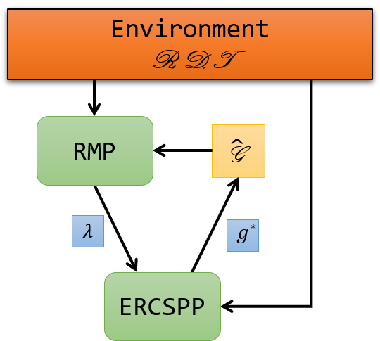
The RMP solves the primal and delivers the dual variables () to the ERCSPP pricing algorithm. The pricing algorithm solves the ERCSPP and delivers the optimal route(s) found (). The set of columns is updated to include the new route(s), and the new set is inputted to the RMP to be resolved. The environment passes its relevant parameters (items, time windows, and extant robots) to the necessary modules.
5 Dual Optimal Inequalities
In this section, we provide dual optimal inequalities (DOI) for MRR, which accelerate CG and motivate better approximate solutions at termination of CG when the LP relaxation is loose. Our DOI are motivated by the following observation. No optimal solution to (8) services an item that is associated with a net penalty instead of a net reward for being serviced, meaning that must be observed. This is so because simply not servicing the item but using an identical route in space and time would produce a lower reduced cost route.
Since the dual LP relaxation of (1)-(6) is increasing with respect to , no optimal dual solution to (1)-(6) will violate . By enforcing at each iteration of CG optimization, we accelerate CG by restricting the dual space that needs to be explored. In the primal form, Eq (1) and Eq (2) are altered as follows with primal variables corresponding to .
In our experiments, we use the replacements above when solving the ILP over the column set . When enforcing that is binary, the technique described often leads to a closer approximations to the solution to Eq (1)-(6). We map any solution derived this way to one solving the original ILP by arbitrarily removing over-included items from routes in the output solution until each item is included no more than once.
6 Solving the Pricing Problem
In this section, we consider the problem of pricing, which we show is an elementary resource-constrained shortest-path problem (ERCSPP) (Righini and Salani 2008). We organize this section as follows. In Section 6.1, we formulate pricing as an ERCSPP over a graph whose nodes correspond to space-time positions and whose resources correspond to the items to be picked up. In Section 6.2, we accelerate computation from Section 6.1 by coarsening the graph, leaving only locations of significance (here these are locations containing item to be picked up). In Section 6.3, we further accelerate computation by limiting the times considered while still achieving exact optimization during pricing. In Section 6.4, we show that CG can be accelerated by updating the for all more often than the remainder of the dual solution, saving computation time by eliminating the need to reconstruct the coarsened graph between each round of pricing.
6.1 Basic Pricing
In this section we establish a weighted graph admitting an injunction from the routes in to the paths in the graph. By that we mean that every route corresponds to at most one path, but paths do not necessarily correspond to routes (and in fact most do not). For a given route , the sum of the weights along the corresponding path in the weighted graph is equal to the route’s reduced cost . Thus finding the highest-profit feasible (where feasible means corresponding to a member of ) path in this graph solves (8). The graph proposed is a modified form of the time-extended graph . Nodes are added to represent start/end locations, item pickups, and the use of extant robots. Remember that extant robots can begin at any location in the graph and that they can have reduced carrying capacities due to items that have already been picked up. Weights are amended by the corresponding dual variables associated with a given node/edge. We solve an ERCSPP over this graph where the resources are the items to be picked up.
Formally, consider a graph with paths described by for , where indicates that edge is traversed by the path on the graph corresponding to route .
Each edge has an associated weight . There is a node in for each , for each pairing of and denoted , for each denoted , the source node , and the sink node . We ensure that for all .
For each pair of space-time positions occurring at the same cell at times (representing a wait action), we set . We set IFF robot route transfers from to and no pickup is made at .
For each pair of space-time positions occurring at times and and associated with space-time edge (representing a move action), we set . We set IFF robot route transfers from to and no pickup is made at .
For each , which occurs at space-time position , we set . We set IFF robot route picks up item at time .
For each , which occurs at an associated , we provide identical outgoing terms for as we do (except there is no self connection to ). We set IFF robot route transfers from the position of item to and item is picked up at time on route .
For each we connect the to the launcher at time denoted with weight . We set IFF the robot route appears first at .
For each we set . We set IFF the robot route appears first at . For each , has one single outgoing connection to with weight .
For each we set . We set IFF the robot route has its last position at .
Using defined above we express the solution to (8) as an ILP ( followed by description) using decision variables where is equal to for all .
| (9) | |||
| (10) | |||
| (11) | |||
| (12) |
In (9) we provide objective s.t. for all . In (10) we ensure that describes a path from to across space and time. In (11) we ensure that capacity is obeyed. In (12) we ensure that each item is picked up at most once. Optimization in (9)-(12) is strongly NP-hard as complexity grows exponentially with (Desrochers et al. 1992).
6.2 Efficient Pricing: Considering Only Nodes Corresponding to Items
In this section we rewrite the optimization for pricing in a manner that vastly decreases the size of the graph under consideration. This transformation leads to efficient optimal solutions for the ERCSPP. We exploit the fact that given the space-time positions where item pickups occur, we can solve of the remainder of the problem as independent parts. Each such independent part is solved as a simple shortest path problem, which can be solved via a shortest path algorithm such as Dijkstra’s algorithm (Dijkstra et al. 1959).
We now consider a graph with node set with edge set , decision and weights . There is one node in for each excluding those for , i.e., . For any , IFF there exists a path from to in traversing only intermediate nodes that exist in . We set to be the weight of the shortest path from to in using only intermediate nodes in . This is easily computed using a shortest path algorithm. We set IFF is followed by in robot route when ignoring nodes in . Replacing with respectively in (9)-(12) we have a smaller but equivalent optimization problem permitting more efficient optimization.
6.3 More Efficient Pricing: Avoiding Explicit Consideration of All Time Instances
The optimization in Eq (9)-(12) over requires the enumeration of all pairs, which is expensive. In this section we circumvent the enumeration of all pairs by aggregating time into sets in such a manner so as to ensure exact optimization during pricing. Here we draw on the insights discussed in (Boland et al. 2017) with respect to continuous-time service network design problems.
For every , we construct , which is an ordered subset of the times where initially includes and and is augmented as needed.
We order these in time where is the ’th value ordered from earliest to latest.
defines a partition of the window into sets, where the ’th set is defined by .
We use to define the graph and solution mapping. Here consists of and one node for each .
We define if route services item at a time in as its first pick up. The remaining terms are defined similarly over aggregated time sets.
We assign each to be some maximum over the possible paths in associated with .
We set for all . We set .
We set .
For any pair of unique and windows
we set .
Evaluating each of the terms amounts to solving a basic shortest path problem (no resource constraints), meaning not all terms mentioned in these optimizations need be explicitly computed.
Replacing with in (9)-(12) we have a much smaller problem permitting more efficient optimization, which provides a lower bound on (9)-(12).
Optimization produces a feasible route when each item in the route is associated with exactly one unique time. In pursuit of a feasible route, we add the times associated with items in the route to their respective sets.
We iterate between solving the ERCSPP over and augmenting the until we obtain a feasible route. This must ultimately occur since eventually would include all for all ; though termination occurs much earlier in practice.
We describe pricing formally below. We use and to denote the maximizers
used to calculate .
The term is the time component maximizer for while is the time component maximizer for . These are the outgoing and incoming times, respectively, for the shortest path on between and .
We use tot_sz to keep track of the total number of elements in all sets. A growth in tot_sz implies a mismatch between the incoming time and the outgoing time at an item location. In such cases, tot_sz grows to narrow the time ranges for the sets, making it less likely to have a mismatch. When tot_sz does not grow, no mismatch occurred and the solution obtained represents a feasible route, therefore we terminate pricing.
6.4 Partial Optimization of the Restricted Master Problem for Faster Pricing
Solving the pricing problem is the key bottleneck in computation experimentally. One key time consumer in pricing is the computation of the terms, which can easily be avoided by observing that terms are offset by changes in and but the actual route does not change so long as , , and are fixed. We resolve the RMP fully only periodically so that we can perform several rounds of pricing using different terms leaving the fixed.
7 Heuristic Pricing
To accelerate CG in operations research applications, one often solves the pricing problem approximately and efficiently instead of solving pricing exactly (Danna and Le Pape (2005), Costa et al. (2019)). When heuristic pricing fails to produce a negative reduced cost column, an exact algorithm can then be called for pricing; thus in the end, the use of heuristic pricing need not lead to sacrificing the guarantees of exact inference. Heuristic pricing can also be used in problems where exact pricing is intractable but can be solved heuristically very well and efficiently ((Lokhande et al. 2020)).
In this section we propose a heuristic pricing approach to solving the selection of the optimal route in that exploits the following observation. Given any ordering of the item set , computing the lowest reduced cost column that is consistent with that ordering is computationally tractable. We express this mathematically as follows.
We use to denote the set of orderings of , which we index by .
We describe using where IFF precedes directly or indirectly in ordering .
We use to denote the subset of consistent with ordering .
The lowest reduced cost path evaluated on graph () respecting the ordering enforces the following
| (13) | |||
Since (13) enforces that no item is repeated in a route we can remove (12) from consideration when solving . We now write given as a polynomial time solvable dynamic program.
Let us define as the subset of s.t. . Let us define for any given the value as the cost of the lowest cost path in starting at and ending at , requiring exactly units of demand.
We define recursively below.
| (14) | |||
Since each execution of (14) is fast we solve (14) using multiple different random orderings and retain the solution with lowest reduced cost.
We now study the probability that our heuristic pricing algorithm produces the lowest reduced cost route when run multiple times. Specifically we show that given capacity , and random orderings that we compute the lowest reduced cost route with probability where .
We establish this as follows. Consider any random ordering of the items and route . Since all orderings are equally likely then the probability that any given route containing items follows the ordering in is . Since the number of items in the lowest reduced cost route is no greater than then the probability that a random ordering supports is no less than . If we generate random orderings (with replacement) the probability that any one of those orderings is consistent with is 1- the probability that none are consistent with or .
In our experiments the units of demand at each pickup location can be . The carrying capacity of each robot, , is set to 6 units.
If we run 25 rounds of heuristic pricing in each attempt to solve in Algorithm 2, then we have a probability of finding the lowest reduced cost column which includes 1 through 6 stops (1,2,3,4,5,6), [1, 1, 0.9858, 0.6549, 0.1888, 0.03415] respectively.
It should be noted that since our heuristic algorithm employs a dynamic program, each ordering that is solved can produce multiple negative reduced cost routes. We also get multiple routes from solving over multiple orderings. CG convergence is often accelerated by returning multiple columns through each iteration. In practice we choose to return a designated number of columns from the union of negative reduced cost columns obtained over all orderings.
8 Experiments
We run two separate experiments to study our model. In the first one, we study the added value of our model, comparing it to a modified version employing MAPF. In the second one, we study the speedup obtained by employing our heuristic pricing algorithm. We evaluate on benchmark maps used in the MAPF literature and on synthetically generated maps.
For problems on benchmark maps, we generate instances by randomly assigning pickup items, and extant robot initial locations, to locations on the map. We set the launcher point to be a central position on the map. For synthetically generated maps, we generate problems by starting with an open, square grid and randomly positioning a set number of obstacles throughout the grid space. In these synthetic problems, items, extant robots, and the launcher have randomly assigned positions.
If we require an exact solution to the ERCSPP during pricing, we do so using an exponential time dynamic program outlined in the next section (8.1). Similar to heuristic pricing, the algorithm is capable of returning multiple negative reduced cost columns, the optimal one being among them. We set the maximum number of columns delivered when using either heuristic or exact pricing as a problem parameter. We return the lowest reduced cost columns when more are available than can be returned.
We update the Lagrangian multipliers , , , and the associated graph components every three CG iterations, unless we are unable to find a negative reduced cost column in a given iteration, in which case we update all dual variables and rerun pricing. If, immediately after all dual variables are optimized, pricing fails to find a negative reduced cost column, then we have finished optimization and conclude CG. To ensure feasibility for the initial round of CG, we initialize the RMP with a prohibitively high cost dummy route for each , where all but . These dummy routes represent an active robot route for each , and thus guarantee that (4) is satisfied. These extra robots ensure feasibility, but are not active at termination of CG due to their prohibitively high cost. Experiments are run in MATLAB, and CPLEX is used as our general purpose (mixed integer) linear programming solver. Our machine is equipped with a 8-core AMD Ryzen 1700 CPU @3.0 GHz and 32 GB of memory running Windows 10.
A sample problem with the solution routes is shown in Figure 3. Each plot in the Figure 3 shows a snapshot in time of the same instance’s solution. A snapshot shows each robot’s route from the initial time up to the time of the snapshot.

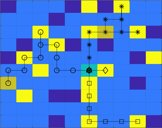
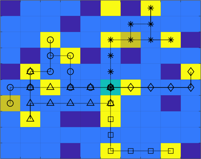

(Left): t = 8 snapshot
(Middle): t = 16 snapshot
(Right): t = 30 (end time) snapshot
8.1 Elementary Resource-Constrained Shortest-Path Solver
We solve the elementary resource-constrained shortest-path problem (ERCSPP) in pricing via an exponential time dynamic program that iterates over the possible remaining capacity levels for a robot (starting at the highest), enumerating all available routes corresponding to paths in at each capacity level, and then progressing to the next highest remaining capacity level. At each level, we eliminate any inferior routes. We call a route inferior to another IFF all of the following are satisfied: (1) it has the same remaining capacity and corresponding position in the node set as the other, (2) it has higher cumulative edge profit on than the other, and (3) it has a set of serviceable items available to it that is a subset of the other’s.
We start at the maximum robot capacity and enumerate all possible single visit traversals. We save a robot state for each such route. A robot state is defined by its current corresponding position in the node set , the items serviced, the cost incurred so far on , and the remaining capacity. We set to be the cost of a path at graph position with path history , a set of all previously visited graph positions. We set to be the remaining capacity available for a robot at corresponding graph position with history . For a robot route with initial visit at item at corresponding graph position we have the following remaining capacity and cost.
| (15) | |||
| (16) |
We then move on to the next highest remaining robot capacity level. For each saved robot state at this remaining capacity, we enumerate all available single visit traversals (including back to the launcher) and save a state for each route generated. An item is available to be visited if that item has not yet been visited in the route and visiting it would not exceed the remaining capacity. For a robot traveling from corresponding graph position with history , to corresponding graph position , we have the following update for the cost and remaining capacity.
| (17) | |||
| (18) |
We eliminate all inferior routes generated and continue on to the next capacity level until we have exhausted all possible remaining capacity levels. At the end, we have series of routes drawn out, including the route with minimum cost on . We can return any number of these that have a negative cost. Returning more serves to reduce the number of CG iterations, but comes with a trade-off of burdening the RMP with more, possibly unnecessary, columns.
8.2 Comparison with MAPF
We compare our algorithm to a modified version that incorporates MAPF. This version will initially ignore robot collision constraints but ultimately considers them after a set of serviceable items are assigned to specific robots. The modified algorithm works as follows. We solve a given problem instance using our CG algorithm, but we neglect the collision constraints, meaning and that the IP solved is defined by equations (1)-(4). This is a vehicle routing problem which delivers us a set of time-window feasible robot routes, including the items serviced by each robot; however, these routes could include collisions. We then take the disjoint set of items serviced (routes) and feed them to a MAPF solver (Li et al. 2021) employing Priority Based Search (Ma et al. 2019). The MAPF solver delivers a set of non-colliding robot routes, each attempting to service the set of items assigned to it. If the MAPF solver fails to provide a valid route for a particular robot (i.e., it cannot make it back to the launcher in time) that route is excluded in the algorithm’s final solution. Since standard MAPF solvers can not handle time windows on items we ignore the time windows for the MAPF solver, but not our CG solver. This provides an advantage to the MAPF solver by permitting it to use routes that do not obey time windows associated with items. When we say permitting here, we need to clarify. The ordered disjoint sets are time-window feasible, but by eliminating collisions (causing robots to wait enroute) we could produce routes which are then time-window infeasible (but not by much since the original routes are time-window feasible). We do not worry about this issue – only that the robots return to the launcher by the end of the time period.
We compare the resulting objective values from our full CG approach to this modified approach. We solve 25 instances on the 32x32 grid maze-32-32-2 that was presented recently in (Stern et al. 2019). Each problem instance has 60 pickup items (of size 1-3), 8 total robots, 2 extant robots, and 150 total time steps. We set to -1, to -1, and the reward for servicing any item, , to 100. Each robot, including the extant ones, has a capacity of 6, while each item has a random size (capacity consumption) uniformly distributed over the set {1,2,3} units. Note that this choice is arbitrary. We could also set the capacity of each extant robot to be random integer between 1 and 6. In each round of pricing we return the 50 lowest reduced cost columns found. Each item’s time window is randomly set uniformly over the available times and can be up to 50 time periods wide. We compare our final results with time windows to the MAPF algorithm’s results without them. The objective value results for both approaches are show in table 1. A side by side plot of the objective values is shown in Figure 4.
| CG | modified CG + MAPF | Difference (CG - MAPF) | Relative Difference | |
|---|---|---|---|---|
| mean | 2230.1 | 1555.5 | 674.6 | 30.21 |
| median | 2202.0 | 1535.0 | 685.0 | 31.10 |
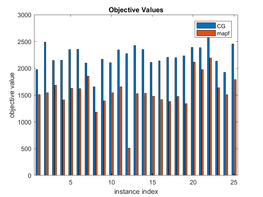
We see an average objective difference of 921 revenue units and a median difference of 782 revenue units from the modified algorithm to our full algorithm. We note from looking at Figure 4 that each of the 25 instances show drastic improvements for our algorithm. These instances largely include robot routes that the MAPF algorithm was unable to find a complete route for within the time constraint given the potential collisions with other robots. With such problems we see it is critical to employ our full algorithm that jointly considers routing and assignment.
Runtime results, iteration counts, and objective values for our full CG approach on the 25 problem instances are shown in Table 2. We also look at the LP objective of the CG solution and the corresponding relative gaps. The relative gap is defined as the the absolute difference between the upper bound (the LP objective value) and our integer solution (the lower bound) divided by the upper bound. We normalize so as to efficiently compare the gap obtained (upper bound - lower bound) across varying problem instances. Please note that the runtimes are of theoretical interest only. In practice we would use the heuristic pricing speedup discussed in the next section.
| Time (sec) | Iterations | LP Objective | Integral Objective | Relative Gap | |
| mean | 17577.5 | 65.9 | 2347.6 | 2230.1 | .05 |
| median | 6526.1 | 67 | 2289.8 | 2202.0 | .05 |
8.3 Heuristic Pricing Speedup
There is no question that without further improvements, the CG solver is too slow to work in practice. However we find that our heuristic pricing yields considerable speedup. We run experiments to measure the speedup offered by our heuristic pricing solver. We compare two approaches. In the first approach, we employ heuristic pricing in each iteration but ultimately employ exact pricing if heuristic pricing fails in any iteration. In this scenario, exact pricing must be employed at least once in order to ensure optimality of the LP solution. In the second approach, we employ exact pricing at each iteration. We solve on random problem instances with randomly generated grids. Each experiment is run on a 25x25 grid with 50 random obstacles, 5 total robots, 2 extant robots, and 75 time steps. Robots have a capacity of 6 while each pickup item has a uniform random demand in the set . is set to 100 while and are both set to -1. Each item’s time window is randomly set uniformly over the available times and can be up to 25 time periods wide. We return the lowest 25 reduced cost columns found when employing heuristic or exact pricing. We run this problem setup for different pickup item counts ranging from 10 to 30 in increments of 5. For each pickup item count, we run 10 random instances and record the average runtime over the instances. Numerical results are shown in Table 3 and a corresponding plot is shown in Figure 5.
| D | EP | HP | speedup (x) |
|---|---|---|---|
| 10 | 56.1 | 25.5 | 2.1 |
| 15 | 192.2 | 55.7 | 3.4 |
| 20 | 826.8 | 114.4 | 6.8 |
| 25 | 2605.9 | 211.8 | 10.7 |
| 30 | 4989.0 | 346.1 | 13.1 |
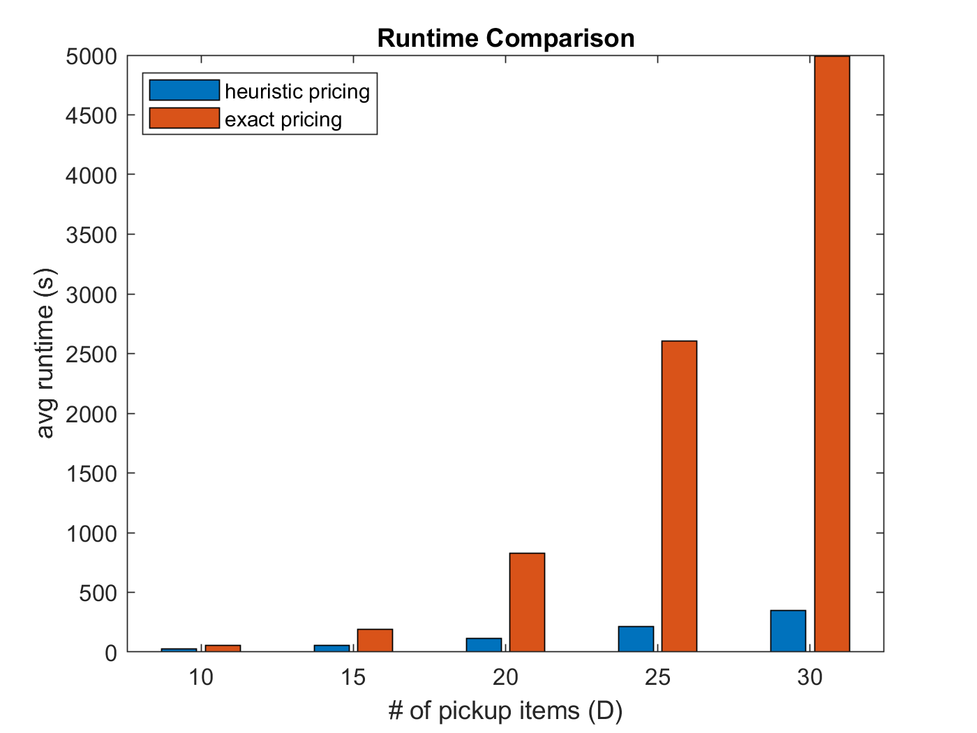
It can be observed that employing heuristic pricing offers a positive average speedup for all pickup item counts. This speedup starts small for 10 pickup items, but grows considerably as the number of pickup items is increased. We see that the real value in the heuristic pricing solver is its scalability in comparison to exact pricing. Further speedups would be considered in a practical application of this method, and taken together these would yield impressive time savings. See for example the work of (Desaulniers et al. 2002).
9 Conclusion and Future Research
In this paper, we unified the work on multi-agent path finding with the vehicle routing-column generation literature to produce a novel approach applicable to broad classes of Multi-Robot Routing (MRR) problems. The new decade accelerated an already rapid transformation of many warehouse operations to automation, thereby increasing the importance of these problems as a key factor in agile supply chains. Our work treats MRR as a weighted set packing problem where sets correspond to valid robot routes and elements correspond to space-time positions. Pricing is treated as an elementary resource-constrained shortest-path problem (ERCSPP), which is NP-hard, but solvable in practice (Irnich and Desaulniers 2005). We solve the ERCSPP by adapting the approach of (Boland et al. 2017) to limit the time windows that need be explored during pricing. We introduce a heuristic pricing algorithm to efficiently solve the ERCSPP problem. While this speeds up the processing considerably and probably results in a model which can be implemented on a rolling-horizon basis (with heuristic real-time insertion techniques), further improvement in the pricing problem would be helpful. Our ongoing research shows great promise in this regard.
The easiest future work is to transform this formulation to the closely related problem in which robots collect pallets and move these to staging areas where human or automate pickers select items. These pallets are then returned to the warehouse floor. That version of the MRR problem can easily be solved within our framework.
Our next future task will be to tighten the LP relaxation using subset-row inequalities (Jepsen et al. 2008) and ensure integrality with branch-and-price (Barnhart et al. 1996). Subset row inequalities are trivially applied to sets over the pickup items since they do not alter the solution paths. Similarly, branch-and-price could be applied to sets over pickup items, following the vehicle routing literature (Desrochers et al. 1992). We also seek to provide insight into the structure of dual optimal solutions and study the effect of smoothing in the dual, based on the ideas of (Haghani et al. 2020b, a). Simply put, we suspect that dual values change smoothly across space and time, thus we will encourage such solutions over the course of column generation. Finally, we intend to apply our column generation solution techniques to a wide variety of transportation and logistics optimization problems.
References
- Appelgren [1969] L. H. Appelgren. A column generation algorithm for a ship scheduling problem. Transportation Science, 3(1):53–68, 1969.
- Appelgren [1971] L. H. Appelgren. Integer programming methods for a vessel scheduling problem. Transportation Science, 5(1):64–78, 1971.
- Azadeh et al. [2019a] K. Azadeh, R. De Koster, and D. Roy. Robotized and automated warehouse systems: Review and recent developments. Transportation Science, 53(4):917–945, 2019a.
- Azadeh et al. [2019b] K. Azadeh, D. Roy, and R. De Koster. Design, modeling, and analysis of vertical robotic storage and retrieval systems. Transportation Science, 53(5):1213–1234, 2019b.
- Barnhart et al. [1996] C. Barnhart, E. L. Johnson, G. L. Nemhauser, M. W. P. Savelsbergh, and P. H. Vance. Branch-and-price: Column generation for solving huge integer programs. Operations Research, 46:316–329, 1996.
- Ben Amor et al. [2006] H. Ben Amor, J. Desrosiers, and J. M. Valério de Carvalho. Dual-optimal inequalities for stabilized column generation. Operations Research, 54(3):454–463, 2006.
- Boland et al. [2017] N. Boland, M. Hewitt, L. Marshall, and M. Savelsbergh. The continuous-time service network design problem. Operations Research, 65(5):1303–1321, 2017.
- Boland et al. [2019] N. Boland, M. Hewitt, L. Marshall, and M. Savelsbergh. The price of discretizing time: a study in service network design. EURO Journal on Transportation and Logistics, 8(2):195–216, 2019.
- Boysen et al. [2019] N. Boysen, R. De Koster, and F. Weidinger. Warehousing in the e-commerce era: A survey. European Journal of Operational Research, 277(2):396–411, 2019.
- Costa et al. [2019] L. Costa, C. Contardo, and G. Desaulniers. Exact branch-price-and-cut algorithms for vehicle routing. Transportation Science, Forthcoming, 2019.
- Custodio and Machado [2020] L. Custodio and R. Machado. Flexible automated warehouse: a literature review and an innovative framework. The International Journal of Advanced Manufacturing Technology, 106(1):533–558, 2020.
- Danna and Le Pape [2005] E. Danna and C. Le Pape. Branch-and-price heuristics: A case study on the vehicle routing problem with time windows. In Column generation, pages 99–129. Springer, 2005.
- Dash et al. [2012] S. Dash, O. Günlük, A. Lodi, and A. Tramontani. A time bucket formulation for the traveling salesman problem with time windows. INFORMS Journal on Computing, 24(1):132–147, 2012.
- Desaulniers et al. [2002] G. Desaulniers, J. Desrosiers, and M. M. Solomon. Accelerating strategies in column generation methods for vehicle routing and crew scheduling problems. In Essays and surveys in metaheuristics, pages 309–324. Springer, 2002.
- Desrochers et al. [1992] M. Desrochers, J. Desrosiers, and M. Solomon. A new optimization algorithm for the vehicle routing problem with time windows. Operations Research, 40(2):342–354, 1992.
- Dijkstra et al. [1959] E. W. Dijkstra et al. A note on two problems in connexion with graphs. Numerische Mathematik, 1(1):269–271, 1959.
- Farinelli et al. [2020] A. Farinelli, A. Contini, and D. Zorzi. Decentralized task assignment for multi-item pickup and delivery in logistic scenarios. In Proceedings of the 19th International Joint Conference on Autonomous Agents and Multi-Agent Systems (AAMAS), pages 1843–1845, 2020.
- Foumani et al. [2018] M. Foumani, A. Moeini, M. Haythorpe, and K. Smith-Miles. A cross-entropy method for optimising robotic automated storage and retrieval systems. International Journal of Production Research, 56(19):6450–6472, 2018.
- Gange et al. [2019] G. Gange, D. Harabor, and P. J. Stuckey. Lazy CBS: Implicit conflict-based search using lazy clause generation. In Proceedings of the 29th International Conference on Automated Planning and Scheduling (ICAPS), pages 155–162, 2019.
- Gilmore and Gomory [1965] P. Gilmore and R. E. Gomory. Multistage cutting stock problems of two and more dimensions. Operations Research, 13(1):94–120, 1965.
- Grenouilleau et al. [2019] F. Grenouilleau, W. van Hoeve, and J. N. Hooker. A multi-label A* algorithm for multi-agent pathfinding. In Proceedings of the 29th International Conference on Automated Planning and Scheduling (ICAPS), pages 181–185, 2019.
- Haghani et al. [2020a] N. Haghani, C. Contardo, and J. Yarkony. Relaxed dual optimal inequalities for relaxed columns: With application to vehicle routing. arXiv preprint arXiv:2004.05499, 2020a.
- Haghani et al. [2020b] N. Haghani, C. Contardo, and J. Yarkony. Smooth and flexible dual optimal inequalities. arXiv preprint arXiv:2001.02267, 2020b.
- Irnich and Desaulniers [2005] S. Irnich and G. Desaulniers. Shortest path problems with resource constraints. In G. Desaulniers, J. Desrosiers, and M. M. Solomon, editors, Column generation, pages 33–65. Springer, 2005.
- Jepsen et al. [2008] M. Jepsen, B. Petersen, S. Spoorendonk, and D. Pisinger. Subset-row inequalities applied to the vehicle-routing problem with time windows. Operations Research, 56(2):497–511, 2008.
- Lam et al. [2019] E. Lam, P. Le Bodic, D. Harabor, and P. J. Stuckey. Branch-and-cut-and-price for multi-agent pathfinding. In Proceedings of the 28th International Joint Conference on Artificial Intelligence (IJCAI), pages 1289–1296, 2019.
- Levin [1971] A. Levin. Scheduling and fleet routing models for transportation systems. Transportation Science, 5(3):232–255, 1971.
- Li et al. [2020] J. Li, G. Gange, D. Harabor, P. J. Stuckey, H. Ma, and S. Koenig. New techniques for pairwise symmetry breaking in multi-agent path finding. In Proceedings of the 30th International Conference on Automated Planning and Scheduling (ICAPS), 2020.
- Li et al. [2021] J. Li, A. Tinka, S. Kiesel, J. W. Durham, T. K. S. Kumar, and S. Koenig. Lifelong multi-agent path finding in large-scale warehouses. In Proceedings of the 35th AAAI Conference on Artificial Intelligence (AAAI), 2021.
- Liu et al. [2019] M. Liu, H. Ma, J. Li, and S. Koenig. Task and path planning for multi-agent pickup and delivery. In Proceedings of the 18th International Joint Conference on Autonomous Agents and Multi-Agent Systems (AAMAS), pages 1152–1160, 2019.
- Lokhande et al. [2020] V. S. Lokhande, S. Wang, M. Singh, and J. Yarkony. Accelerating column generation via flexible dual optimal inequalities with application to entity resolution, 2020.
- Lübbecke [2010] M. E. Lübbecke. Column generation. Wiley Encyclopedia of Operations Research and Management Science, 2010.
- Lübbecke and Desrosiers [2005] M. E. Lübbecke and J. Desrosiers. Selected topics in column generation. Operations Research, 53(6):1007–1023, 2005.
- Ma et al. [2017] H. Ma, J. Li, T. K. S. Kumar, and S. Koenig. Lifelong multi-agent path finding for online pickup and delivery tasks. In Proceedings of the 16th International Conference on Autonomous Agents and Multi-Agent Systems (AAMAS), pages 837–845, 2017.
- Ma et al. [2019] H. Ma, D. Harabor, P. J. Stuckey, J. Li, and S. Koenig. Searching with consistent prioritization for multi-agent path finding. In Proceedings of the AAAI Conference on Artificial Intelligence, volume 33, pages 7643–7650, 2019.
- Righini and Salani [2008] G. Righini and M. Salani. New dynamic programming algorithms for the resource constrained elementary shortest path problem. Networks: An International Journal, 51(3):155–170, 2008.
- Sánchez et al. [2020] M. Sánchez, J. M. Cruz-Duarte, J. carlos Ortíz-Bayliss, H. Ceballos, H. Terashima-Marin, and I. Amaya. A systematic review of hyper-heuristics on combinatorial optimization problems. IEEE Access, 8:128068–128095, 2020.
- Shekari Ashgzari and Gue [2021] M. Shekari Ashgzari and K. R. Gue. A puzzle-based material handling system for order picking. International Transactions in Operational Research, 2021.
- Stenger et al. [2013] A. Stenger, M. Schneider, and D. Goeke. The prize-collecting vehicle routing problem with single and multiple depots and non-linear cost. EURO Journal on Transportation and Logistics, 2(1-2):57–87, 2013.
- Stern et al. [2019] R. Stern, N. R. Sturtevant, A. Felner, S. Koenig, H. Ma, T. T. Walker, J. Li, D. Atzmon, L. Cohen, T. K. S. Kumar, R. Barták, and E. Boyarski. Multi-agent pathfinding: Definitions, variants, and benchmarks. In Proceedings of the 12th International Symposium on Combinatorial Search (SoCS), pages 151–159, 2019.
- Surynek [2019] P. Surynek. Unifying search-based and compilation-based approaches to multi-agent path finding through satisfiability modulo theories. In Proceedings of the 28th International Joint Conference on Artificial Intelligence (IJCAI), pages 1177–1183, 2019.
- Wang and Regan [2002] X. Wang and A. C. Regan. Local truckload pickup and delivery with hard time window constraints. Transportation Research Part B: Methodological, 36(2):97–112, 2002.
- Wang and Regan [2009] X. Wang and A. C. Regan. On the convergence of a new time window discretization method for the traveling salesman problem with time window constraints. Computers & Industrial Engineering, 56(1):161–164, 2009.
- Weidinger et al. [2018] F. Weidinger, N. Boysen, and D. Briskorn. Storage assignment with rack-moving mobile robots in kiva warehouses. Transportation science, 52(6):1479–1495, 2018.
- Yarkony et al. [2020] J. Yarkony, Y. Adulyasak, M. Singh, and G. Desaulniers. Data association via set packing for computer vision applications. Informs Journal on Optimization, 2(3):167–191, 2020.
- Yu and LaValle [2013] J. Yu and S. M. LaValle. Planning optimal paths for multiple robots on graphs. In Proceedings of the IEEE International Conference on Robotics and Automation (ICRA), pages 3612–3617, 2013.
- Zhang et al. [2017] C. Zhang, S. Wang, M. A. Gonzalez-Ballester, and J. Yarkony. Efficient column generation for cell detection and segmentation. arXiv preprint arXiv:1709.07337, 2017.