Planckian Metal at a Doping-Induced Quantum Critical Point

Abstract

We numerically study a model of interacting spin-$1/2$ electrons with random exchange coupling on a fully connected lattice. This model hosts a quantum critical point separating two distinct metallic phases as a function of doping: a Fermi liquid phase with a large Fermi surface volume and a low-doping phase with local moments ordering into a spin-glass. We show that this quantum critical point has non-Fermi liquid properties characterized by $T$-linear Planckian behavior, $\omega/T$ scaling and slow spin dynamics of the Sachdev-Ye-Kitaev (SYK) type. The $\omega/T$ scaling function associated with the electronic self-energy is found to have an intrinsic particle-hole asymmetry, a hallmark of a ‘skewed’ non-Fermi liquid.

The normal-state properties of hole-doped cuprates are fundamentally different on the two sides of the critical doping $p=p^{\star}$ at which the pseudogap opens. For $p>p^{\star}$ the Fermi surface (FS) is large and consistent with band structure predictions [1, 2]. In contrast, for $p<p^{\star}$ there is clear experimental evidence that a transformation to a ‘small’ FS takes place [3, 2, 4]. The vicinity of $p^{\star}$ hosts a ‘strange metal’ in which resistivity is linear in temperature $T$ down to low-$T$ (for reviews, see [5, 6, 7]). Hallmarks of quantum criticality [8] have been reported in this regime including $\omega/T$ scaling in spectroscopy experiments [9, 10]. The nature of the $p<p^{\star}$ phase and that of the strange metal are outstanding fundamental questions.

Microscopic models that exhibit such a doping-induced quantum critical point (QCP) and can also be investigated in a controlled manner are rare. In early pioneering work, Sachdev and Ye [11] showed that the random-bond fully connected quantum Heisenberg model hosts a spin-liquid phase when solved for $SU(M)$ spins in the large-$M$ limit. Remarkably, the local spin dynamics in this phase has the characteristic frequency dependence of a marginal Fermi liquid [12, 13, 7] and obeys $\omega/T$ scaling as a consequence of conformal invariance [14]. A generalization to a $t$-$J$ model including itinerant charge carriers was introduced by two of the present authors [14] (see also [15, 16, 17, 18]), who found that in the large-$M$ limit there is a QCP at zero doping. The doped metal was found to be a Fermi liquid (FL) at low-$T$, with a higher-$T$ quantum-critical regime corresponding to a ‘bad metal’ [19, 20, 21, 22, 23] with $T$-linear resistivity larger than the Mott-Ioffe-Regel value.

Triggered by widespread interest in the broader Sachdev-Ye-Kitaev (SYK) framework and duality to quantum gravity [24, 25, 26], this line of research has recently been substantially revived [27, 28, 29, 30, 31]. The realistic case of spin-$1/2$ $SU(2)$ electrons is much richer than the large-$M$ limit considered in early works (see however [29, 30]). Unlike the large-$M$ model, the undoped $SU(2)$ insulator has a spin glass ground-state and a finite ordering temperature [32, 33, 34]. At half-filling, the QCP associated with the melting of this spin-glass phase by charge fluctuations was recently studied in Ref. [27]. It has been shown that the $SU(2)$ doped model hosts a QCP at a finite critical doping $p=p_{c}$ [35, 28, 31]. Understanding the properties of this QCP and whether it shares some of the properties of cuprate phenomenology despite the highly simplified character of the model is a fundamental and fascinating question which is currently being actively investigated [31, 29, 30].

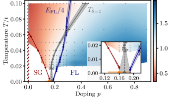
Figure 1: Phase diagram in temperature $T$ and doping $p$. A quantum critical point (QCP; orange dot) separates a spin-glass ordered phase (SG) at low $p$ from a Fermi liquid (FL) at large $p$. Both the SG transition temperature (dark red) and the characteristic FL scale $E_{\mathrm{FL}}/4$ (dark blue) collapse at or near the QCP. The background color corresponds to the power $\theta$ of the long-time spin correlation; the dark grey data and line demarcate $\theta=1$. Pale grey dots indicate parameter values at which calculations were performed. Dashed lines are extrapolations outside the available temperature range. Inset: close-up of the QCP.

In this article, we show that the quantum critical regime associated with the finite doping QCP hosts a strange metal in which the lifetime of excitations shows ‘Planckian’ behavior $1/\tau^{\star}=c\,k_{B}T/\hbar$, with $c$ of order unity [36, 37, 38, 39, 40, 7, 41]. Furthermore, we demonstrate $\omega/T$ scaling of both the local spin dynamics, which is found to be of SYK type as in the undoped case [27], and of the single-particle properties such as the frequency-dependent scattering rate. In the accessible range of temperature, the latter is found to display a particle-hole asymmetry which also scales with $\omega/T$ (‘skewed’ non-Fermi liquid [42]). We establish the phase diagram displayed in Fig. 1. At high doping and low-$T$, the metallic phase is a FL, with a crossover into Planckian behavior in the quantum critical regime. At the QCP the volume of the FS changes abruptly and the system transitions from a FL to another metallic state which is unstable to spin-glass ordering below the indicated critical temperature. These results are established using the extended dynamical mean-field theory (EDMFT) framework [43, 44, 45, 46, 47] and a quantum Monte Carlo algorithm [48, 49], allowing us to study disorder-averaged quantities directly in the thermodynamic limit. In this regard, our study provides a complementary perspective on the quantum critical regime to the recent parallel work by Shackleton et. al. [31] which uses exact diagonalization of finite-size systems for a fixed configuration of disorder.

Model – We consider spin-1/2 electrons on a fully connected lattice governed by the Hamiltonian

$$H=H_{0}+\sum_{i<j}{J_{ij}\boldsymbol{S}_{i}\cdot\boldsymbol{S}_{j}}+U\sum_{i}n_{i\uparrow}n_{i\downarrow},$$ (1)

where $H_{0}=-\sum_{ij,\sigma}(t_{ij}+\mu\delta_{ij})c^{{\dagger}}_{i\sigma}c^{{\phantom{\dagger}}}_{j\sigma}$. Here $\sigma=\uparrow,\downarrow$ is the spin-state, $\mu$ is the chemical potential, $n_{i\sigma}=c^{{\dagger}}_{i\sigma}c^{{\phantom{\dagger}}}_{i\sigma}$ is the occupation number on site $i$ with spin-state $\sigma$, and $\boldsymbol{S}_{i}=\tfrac{1}{2}c^{{\dagger}}_{i\sigma^{\prime}}\boldsymbol{\sigma}_{\sigma^{\prime}\sigma}c^{{\phantom{\dagger}}}_{i\sigma}$ is the spin operator on site $i$. The hopping amplitudes $t_{ij}$ are complex with $t_{ij}=t^{*}_{ji}$, and the exchange coupling strengths $J_{ij}$ are real. They are drawn according to independent Gaussian distributions with zero means $\overline{t_{ij}}=\overline{J_{ij}}=0$ and variances $\overline{|t_{ij}|^{2}}=t^{2}/\mathcal{N}$, $\overline{|J_{ij}|^{2}}=J^{2}/\mathcal{N}$. Here, $\mathcal{N}$ is the number of lattice sites and we work directly in the thermodynamic limit $\mathcal{N}\to\infty$, keeping $t,J,U$ finite [50]. We use the replica method to deal with the quenched disorder and we restrict ourselves to replica diagonal paramagnetic solutions without spin-symmetry breaking.

The local electron and spin correlation functions of Eq. (1) are obtained by solving an auxiliary quantum ‘impurity’ model (EDMFT equations) [43, 44, 45, 46, 47, 14, 27]

$$S_{\mathrm{eff}}=\int\!\!\mathrm{d}\tau\left[\sum_{\sigma}c^{\dagger}_{\tau,\sigma}\left[\partial_{\tau}-\mu\right]c^{\phantom{\dagger}}_{\tau,\sigma}+Un_{\tau,\uparrow}n_{\tau,\downarrow}\right]+\\ \int\!\!\mathrm{d}\tau^{\prime}\mathrm{d}\tau\!\left[\Delta(\tau^{\prime}-\tau)c^{\dagger}_{\tau^{\prime},\sigma}c^{\phantom{\dagger}}_{\tau,\sigma}-\frac{J^{2}Q(\tau^{\prime}-\tau)}{2}\boldsymbol{S}_{\tau^{\prime}}\cdot\boldsymbol{S}_{\tau}\right]\!\!$$ (2)

subject to the self-consistency conditions $\Delta(\tau)=t^{2}G(\tau)$ and $Q(\tau-\tau^{\prime})=\tfrac{1}{3}\langle\boldsymbol{S}(\tau)\cdot\boldsymbol{S}(\tau^{\prime})\rangle$. Here we denote imaginary time by $\tau\in[0,\beta]$ and inverse temperature by $\beta=1/T$ ($k_{B}=1$ unless otherwise noted). The self-consistency conditions relate the fermionic hybridization bath $\Delta$ to the local fermionic Green function $G(\tau)=-\langle T_{\tau}c(\tau)c^{\dagger}(0)\rangle$ and the retarded spin-spin interaction $Q$ to the local spin correlation function. The electronic self-energy of the impurity model $\Sigma(i\omega_{n})=i\omega_{n}+\mu-\Delta(i\omega_{n})-G^{-1}(i\omega_{n})$, where $\omega_{n}=(2n+1)\pi/\beta$ are fermionic Matsubara frequencies, coincides with the self-energy of model Eq. (1). Therefore, we can reconstruct the Green function of the lattice model $G_{\mathrm{latt}}^{-1}(\varepsilon,i\omega_{n})=i\omega_{n}+\mu-\varepsilon-\Sigma(i\omega_{n})$, where $\varepsilon$ is an eigenvalue of the random matrix $t_{ij}$ (see App. .2). In the thermodynamic limit, these eigenvalues $\varepsilon$ are distributed according to the Wigner semi-circle law and the local $G$ and $\Sigma$ are self-averaging in the paramagnetic phase [47, 31, 49]. The impurity model is solved using a quantum Monte Carlo interaction-expansion impurity solver in continuous imaginary time (CT-INT) [48, 27], for details see App. .1. Throughout, we set the interaction strengths $J=0.5t$ and $U=4t$ – sufficiently strong to realize the finite doping QCP [27], while still amenable to CT-INT simulations.

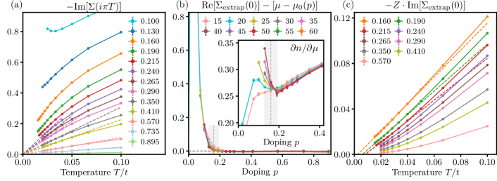
Figure 2: (a) Imaginary component of the self-energy at the first Matsubara frequency $\textrm{Im}[\Sigma(i\pi T)]$, for various doping levels $p$ from $0.1$ to $0.895$. The dashed lines emphasize the low $T$-linear regime which characterizes the Fermi liquid. (b) Violation of the Luttinger theorem at the QCP. The quantity $\textrm{Re}\Sigma_{\mathrm{extrap}}(0)-[\mu-\mu_{0}(p)]$ vs $p$ for various temperatures $15\leq\beta\leq 60$ – it vanishes at low $T$ in the high doping Fermi liquid phase. The doping $p_{c}$ where it deviates from zero defines the QCP (vertical dashed line). Inset: Electronic compressibility $\chi_{e}=\partial n/\partial\mu$. (c) Inverse lifetime $1/\tau^{\star}=-Z\textrm{Im}[\Sigma_{\mathrm{extrap}}(0)]$ (see App. .4). It has a Fermi liquid $T^{2}$ behavior at high doping. Close to the QCP, $p_{c}\approx 0.16-0.19$, it becomes linear in $T$ at low temperatures (dashed lines).

Fermi Liquid – Let us start from the large doping regime. In a FL, $\Sigma(i\omega_{n})$ at low $\omega_{n}$ and $T$ takes the form

$$\textrm{Im}\Sigma(i\omega_{n})=\left(1-\frac{1}{Z}\right)\omega_{n}+\frac{\omega_{n}^{2}-(\pi T)^{2}}{E_{\mathrm{FL}}}+O(T^{3}),$$ (3)

where $Z$ is the quasiparticle weight and $E_{\mathrm{FL}}$ is a characteristic FL scale (see App. .2). Thus, a hallmark of FL behavior is that $\Sigma(i\omega_{n})$ at the first Matsubara frequency depends linearly on $T$: $\textrm{Im}\Sigma(i\pi T)\sim T+O(T^{3})$ [51]. As shown in Fig. 2a, this $T$-linear behavior holds up to a FL crossover-scale $T_{\mathrm{FL}}$, which is large at large doping and decreases with $p$. At $p\leq 0.16$, $\textrm{Im}\Sigma(i\pi T)$ extrapolates to a finite value at $T=0$, signaling a breakdown of FL behavior. We can obtain $E_{\mathrm{FL}}$ and $Z$ from a direct fit of $\textrm{Im}\Sigma(i\omega_{n})$ to Eq. (3). These quantities, together with $T_{\mathrm{FL}}$, collapse at the QCP (see App. .7); see Fig. 1.

A sharp signature of the collapse of the FL at the QCP is the sudden violation of the Luttinger theorem [35], which constrains the volume of the Fermi surface. From the expression of the lattice Green function $G_{\mathrm{latt}}$, the interacting FS is defined by $\varepsilon=\mu-\textrm{Re}\Sigma_{\mathrm{extrap}}(0)$, where $\textrm{Re}\Sigma_{\mathrm{extrap}}(0)$ is the real part of $\Sigma$ extrapolated to zero frequency (see App. .7). Comparing the non-interacting and interacting Fermi surface, Luttinger’s theorem states that $\lim_{T\rightarrow 0}\Delta\varepsilon_{F}(T)=0$, where we define $\Delta\varepsilon_{F}(T)=\textrm{Re}\Sigma_{\mathrm{extrap}}(0)-[\mu-\mu_{0}(p)]$, with $\mu_{0}(p)$ the chemical potential of the non-interacting system $U=J=0$ at the same doping. Figure 2b shows $\Delta\varepsilon_{F}(T)$ versus doping for various temperatures. While for large doping levels, it converges to zero at low temperature as expected for a FL, it clearly does not at low doping. The doping where the deviation onsets, defines the critical point $p_{c}=0.16\pm 0.03$. For $p<p_{c}$ the FL is destroyed and replaced by another metallic phase discussed below.

Planckian behavior. – We now discuss the QCP, approaching it from the high-doping side. Figure 2c shows $1/\tau^{\star}=-Z\textrm{Im}\Sigma_{\mathrm{extrap}}(0)$, which is the width of the spectral function $A(\varepsilon,\omega)=-\mathrm{Im}G(\varepsilon,\omega+i0^{+})/\pi$. In the FL regime $1/\tau^{\star}\propto T^{2}$ and can be interpreted as the inverse of the quasiparticle lifetime. Close to the QCP, FL behavior breaks down and we find a clear ‘Planckian’ behavior [36, 37, 38, 39, 40, 7, 41] down to low-$T$

$$\frac{1}{\tau^{\star}}\simeq c\,\frac{k_{B}T}{\hbar},$$ (4)

restoring fundamental constants. Here $c$ is a coefficient of order unity; $c=1.0\pm 0.1$ for $p=0.19$. Furthermore, the transport scattering rate $1/\tau_{\mathrm{tr}}=-2\textrm{Im}\Sigma_{\mathrm{extrap}}(0)$ is also approximately $T$-linear in this regime (see App. .7). Since the self-energy $\Sigma(\omega)$ is strictly local, the electrical resistivity $\rho$ defined via the Kubo formula (see App. .5) is determined by $1/\tau_{\mathrm{tr}}$. This implies that $\rho$ has an approximately $T$-linear dependence. We emphasize that the resistivity is smaller than the Mott-Ioffe-Regel value at low-$T$, in contrast to ‘bad metal’ behavior. When viewed in terms of Einstein-Sutherland relation $1/\rho=D\,\chi_{e}$ [20, 23, 52, 53], the $T$-linearity of $\rho$ stems from the diffusion constant $D\propto 1/T$, rather than from the compressibility $\chi_{e}=\partial n/\partial\mu$, which has little $T$-dependence at the QCP (Fig. 2b inset).

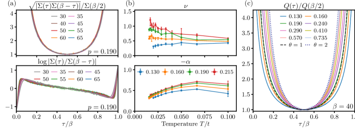
Figure 3: (a) Symmetric (top) and anti-symmetric (bottom) scaling forms of the electronic self-energy in imaginary time $\Sigma(\tau)$ vs $\tau/\beta$. Doping is fixed $p=0.19$ to be near the QCP and we show various $\beta$. (b) Non-Fermi liquid exponent $\nu$ (top) and asymmetry parameter $\alpha$ (bottom), extracted by fitting the scaling form in (a) to Eq. (5), for various doping levels $p$ close to the QCP [50]. (c) Normalized spin-spin correlation $Q(\tau)/Q(\beta/2)$ at a fixed $\beta=40$ and varying $p$. The long imaginary times scaling form $Q(\tau)\sim 1/[\sin(\pi\tau/\beta)]^{\theta}$ is shown with $\theta=2$ (Fermi liquid, dotted line) and $\theta=1$ (SYK, dashed line).

Quantum criticality: skewed non-Fermi liquid and $\omega/T$ scaling. – We now show that our data support $\omega/T$ scaling of the self-energy near the QCP. In real-frequencies, we expect a scaling form $-\textrm{Im}\Sigma(\omega+i0^{+})\propto T^{\nu}\sigma(\omega/T)$ with $\nu$ an exponent ($\nu=2$ for a Fermi liquid). This translates in imaginary time to $\Sigma(\tau)/\Sigma(\beta/2)=\overline{\Sigma}(\overline{\tau})$ with $\overline{\tau}=\tau/\beta$. In order to test this scaling form and identify the scaling function $\overline{\Sigma}$, we plot in Fig. 3a $\sqrt{|\Sigma(\tau)\Sigma(\beta-\tau)|}/\Sigma(\beta/2)$ and $\log|\Sigma(\tau)/\Sigma(\beta-\tau)|$ for several $\beta$ and a fixed $p=0.19$ close to $p_{c}$. This allows to address separately the symmetric (even) and antisymmetric (odd) components of $\Sigma$ under particle-hole symmetry $\tau\rightarrow\beta-\tau$ ($\omega\rightarrow-\omega$). Within the range of temperature accessible to our algorithm we obtain a good scaling collapse of the data in the long-time limit around $\overline{\tau}=1/2$ (see App. .7). The scaling function agrees well with the conformally invariant ansatz:

$$\overline{\Sigma}(\overline{\tau})\,=\,\,e^{\alpha(\overline{\tau}-1/2)}\,\left[\frac{1}{\sin\pi\overline{\tau}}\right]^{\nu+1},\qquad\overline{\tau}=\frac{\tau}{\beta}.$$ (5)

Figure 3b displays the values of $\nu$ and $\alpha$ obtained from a fit of the data in Fig. 3a. We note that $\nu$ varies substantially close to the QCP. The marginal Fermi liquid value $\nu=1$ [12, 13, 7] and the $SU(M\rightarrow\infty)$ model value $\nu=1/2$ [11, 14] are both consistent with our data in the low-$T$ limit, but lie at opposite ends of our extrapolated range. We also note that our observed $T$-linear behavior of $1/\tau_{\mathrm{tr}}$ has to arise out of a combination of the finite temperature dependence of the effective $\nu,\alpha$ and prefactor of $\Sigma(\tau)$ (see App. .3).

Remarkably, Fig. 3b shows that at finite-$T$ in the quantum critical region, our model behaves as a ‘skewed’ non-Fermi liquid, with an $\omega/T$ scaling function $\sigma$ displaying an intrinsic particle-hole asymmetry. The latter is encoded in the spectral asymmetry parameter (skew) $\alpha$ of Eq. (5) (see App. .3), which takes rather large values at finite $T$. Whether this asymmetry persists down to zero temperature at the QCP (i.e. $\alpha$ remains finite at $T=0$) is an interesting open question. Recently, such a particle-hole asymmetry in skewed Planckian metals attracted strong interest, from both theory [42] and experiments [54], as a possible explanation of a puzzle regarding the sign and $T$-dependence of the Seebeck coefficient in cuprate superconductors. Measurements of the thermopower of twisted bilayer graphene [55] indicate possible relevance to other materials as well. We also note that the skew is itself of basic theoretical interest; in the large-$M$ limit, there is a fundamental relationship between it and finite entropy density at the QCP [56].

Quantum criticality: SYK spin dynamics – Figure 3c shows the local spin-spin correlation function $Q(\tau)$ at $\beta=1/40$, for several doping levels. In imaginary time, the universal long time scaling is around $\tau=\beta/2$. By comparison to the conformal scaling function [14, 49] $Q(\tau)/Q(\beta/2)\sim 1/\left[\sin(\pi\tau/\beta)\right]^{\theta}$, we see that at the QCP the spin dynamics slows down from the long-time behaviour $\sim 1/\tau^{2}$ characteristic of a Fermi liquid ($\theta=2$) to the SYK dynamics [11] $\sim 1/\tau$ ($\theta=1$). We fit the critical exponent $\theta$ for all $T$ and $p$, and display it as the background color in Fig. 1. This allows us to locate the temperature scale $T_{\theta=1}$ at which $\theta=1$ (Fig. 1, dark grey data), which extrapolates to the quantum critical point $p_{c}$ at low-temperatures within error bars. This critical SYK scaling was also found in a renormalization group analysis [57, 58, 28] and for the undoped model [27].

Low doping metal and spin-glass – The critical doping $p_{c}$ separates a FL at $p>p_{c}$ from a phase of a different nature for $p<p_{c}$. This phase is also metallic – as seen numerically from $G(i\omega_{n})$ at low frequency (see App. .7) – but it has emerging local moments [35]. This is demonstrated by Fig. 4a, which shows $\Delta Q(0)=\chi_{\mathrm{loc}}-Q_{\mathrm{extrap}}(0)$, where $\chi_{\mathrm{loc}}=Q(i\nu_{0})$ is the static local spin susceptibility at the bosonic Matsubara frequency $\nu_{0}=0$ and $Q_{\mathrm{extrap}}(0)$ is the extrapolated value of $Q(i\nu_{n})$ for $\nu_{n}\rightarrow 0$. A local moment $m=\langle S^{z}\rangle$ is associated with a plateau in the spin-spin correlation $Q(\tau)\sim m^{2}$ at long time. Hence, its Fourier transform is $Q(i\nu_{n})=\beta m^{2}\delta_{n,0}+Q_{\mathrm{reg}}(i\nu_{n})$, where $Q_{\mathrm{reg}}$ is a regular (decaying) function, so that $\Delta Q(0)\propto\beta m^{2}$. For $p>p_{c}$, $\Delta Q(0)$ decreases to zero upon cooling, while it grows for $p<p_{c}$, a clear signature of local moments at low $T$. The presence of local moments for $p<p_{c}$ also explains the distinctive change of behavior of the compressibility $\chi_{e}$ through the critical point (Fig. 2b). The $T$-dependence of $\chi_{e}$ is related to the entropy per site $s$ by the Maxwell relation $\partial^{2}s/\partial n^{2}|_{T}=\chi_{e}^{-2}\,\partial\chi_{e}/\partial T|_{n}$. In a local moment phase, we expect $s$ to be finite at $T=0$ (and $\partial^{2}s/\partial n^{2}<0$; see App. .6), while in the FL phase the entropy vanishes as $s\propto\gamma T$. Hence, at fixed $T$, $s(n)$ must have an inflection point $\partial^{2}s/\partial n^{2}=0$, implying that at this density the compressibility must be independent of $T$. This is indeed observed for $p\simeq p_{c}$ on Fig. 2b (inset).

This local moment metallic solution of the paramagnetic EDMFT equations is unstable to spin glass ordering below the critical temperature depicted on Fig 1. The spin-glass susceptibility is given by [59, 60] $\chi_{\mathrm{SG}}\propto\chi_{\mathrm{loc}}^{2}/(1-J^{2}\chi_{\mathrm{loc}}^{2})$. Its $T$-dependence is displayed on Figure 4b, where we plot $\chi_{\mathrm{SG}}^{-1}$ as a function of $\bigl{(}J/\log(J/T)\bigr{)}^{2}$. In this representation, we expect a linear dependence close to the QCP, since we expect from theory that $J\chi_{\mathrm{loc}}\sim\log(J/T)$ at $p=p_{c}$ ($T\ll J$ here) [59]. It is seen that $\chi_{\mathrm{SG}}$ diverges at a finite spin-glass ordering temperature for $p<p_{c}$ (black dots in Fig. 4b). If the logarithmic form of $\chi_{\mathrm{loc}}$ holds to $T=0$ at the QCP, then $\chi_{\mathrm{SG}}$ will diverge at a finite $T$. Therefore, the spin-glass phase extends to $p\gtrsim p_{c}$ at very low $T$, although this effect is below the temperature resolution of the numerical data. Finally, since we restricted ourselves to paramagnetic (replica diagonal) solutions, we do not describe the spin-glass phase itself. We expect the phase to be metallic at non-zero doping.

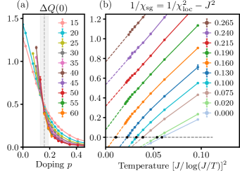
Figure 4: (a) Estimate of local moment component of the spin response $\Delta Q(0)$ (see text). The dashed line marks the QCP $p_{c}$. (b) Inverse of the spin-glass susceptibility $\chi_{\mathrm{sg}}$ vs $\bigl{[}J/\log(J/T)\bigr{]}^{2}$. Black dots mark the extrapolated transition temperature. Dashed lines are linear extrapolations.

Conclusion – The QCP analyzed in this paper separates two distinct metallic phases: a Fermi liquid with a FS volume consistent with Luttinger theorem for $p>p_{c}$ and a phase with local moments and a spin-glass instability for $p<p_{c}$. While being consistent with previous work on this model [35, 28, 31], our study offers new insights into its physical properties. We have shown that a skewed non-Fermi liquid emerges, characterized by $T$-linear ‘Planckian’ behavior, slow SYK spin dynamics, $\omega/T$ scaling and a low-energy particle-hole asymmetry also scaling as $\omega/T$ (‘skew’). It is striking that, despite the extreme simplification of the fully connected $SU(2)$ random $t$-$J$-$U$ model studied here, this is reminiscent of some key aspects of the cuprate phenomenology [9, 7, 6, 2]. We note that recent nuclear magnetic resonance and ultrasound measurements have revealed that, remarkably, the spin-glass phase of La_2-xSr_xCuO₄ extends up to $p=p^{\star}$ in high magnetic fields [61]. We also note that $\omega/T$ scaling of the self-energy has also been reported in ARPES experiments [10]. Our results may be relevant to other materials as well, in which Planckian behavior and quantum criticality are observed, such as twisted bilayer graphene [53, 62]. The ‘skew’ found in our study is of special current interest [42] in relation to the unconventional behavior of the Seebeck coefficient in cuprate superconductors [54] and possibly also twisted bilayer graphene [55].

We thank S. Sachdev, H. Shackleton, A. Wietek as well as P. Cha, E.-A. Kim and J. Mravlje for valuable discussions and collaborations on related work. The algorithms used in this study were implemented using the TRIQS code library [63] and CTINT [64]. The Flatiron Institute is a division of the Simons Foundation.

Appendix

.1 Details of Numerical Simulations

We solve the effective impurity model using the standard dynamical mean field theory (DMFT) approach. In particular, we iteratively solve Eq. (2) and update the hybridization function $\Delta(\tau)=t^{2}G(\tau)$ and the spin-correlation function $Q(\tau)$ until reaching convergence. At each step, we use a quantum Monte Carlo impurity solver in continuous imaginary time, based on perturbative expansion of the partition function in powers of the fermion interaction strength (CT-INT). We refer to the literature for details of the algorithms [48, 65], but note that our implementation [64] extends this approach with a fast computation of $Q(\tau)$ from the three-point vertex function rather than through an operator insertion measurement.

Since the Monte Carlo sampling is performed in the grand canonical ensemble, we adjust the chemical potential $\mu$ between DMFT iterations in order to target a fixed electron density $n$. The iterative procedure converges to a fixed $n$ and $\mu$ alongside the correlation functions. Each calculation is deemed converged when the relative change of $\textrm{Re}G(i\omega_{n})$, $\textrm{Im}G(i\omega_{n})$ and $Q(i\omega_{n})$ between two consecutive iterations is smaller than $1\%$. Note that we apply this convergence only on Fourier modes where there is appreciable weight ($|\textrm{Re}G(i\omega_{n})|>10^{-3},|\textrm{Im}G(i\omega_{n})|>10^{-3}$, or $Q(i\omega_{n})>10^{-2}$) in order to be above the level of statistical noise of the Monte Carlo calculation.

To accelerate the DMFT convergence, we seed the initial configuration for a given $n$ and $T$ from the converged solution at the nearest higher temperature and same density $n$. Since we are only considering paramagnetic solutions in Eq. (2), this annealing procedure is sufficient and we do not consider coexistence or metastability with other orders by construction. Each parameter runs for at least $10$ iterations until convergence and often more – typically $\sim 15$ iterations in the Fermi liquid regime and $\gtrsim 25$ iterations in the regime $p\leq p_{c}$.

Even with these choices, the dominant source of error is still the DMFT convergence error rather than the statistical Monte Carlo error. The error-bars throughout the paper are therefore solely based estimates of this systematic error, obtained by considering the minimum-to-maximum range of values of the observable in the last five DMFT iterations.

.1.1 Alpha Shift

The Monte Carlo sampling we perform suffers from a sign problem, which becomes more pronounced at larger doping. When directly sampling the action Eq. (2) with the parameters studied ($U=4t,J=0.5t$), the sign problem typically limits calculations to high temperatures $\beta\lesssim 20$ in the Fermi liquid regime. To alleviate the sign problem we use a so-called $\alpha$-shift. This changes the origin of the perturbative expansion, by shifting the interaction term of the action by a quadratic term – the Hubbard term becomes $U\sum_{i}(n_{i,\uparrow}-\alpha_{\uparrow})(n_{i,\downarrow}-\alpha_{\downarrow})$ – which is then compensated by a redefinition of the bare propagator; see e.g. Ref. [48] for details. For our model, we found it convenient to use an automated optimization procedure to obtain suitable values for $\alpha_{\uparrow,\downarrow}$. We perform a single iteration calculation with a reduced number of Monte Carlo cycles and use the average sign as our optimization function. Since the Monte Carlo with a low number of measurements has a significant statistical error, we used a Bayesian optimization based on Gaussian processes, since this can naturally treat optimization functions with noisy output. Instead of a full 2d parameter optimization, we found it more efficient to perform 1d optimizations of $\overline{\alpha}=\tfrac{1}{2}(\alpha_{\uparrow}+\alpha_{\downarrow})$ for increasing values of $\delta=\alpha_{\uparrow}-\alpha_{\downarrow}$ until finding values for which the average sign is $>0.37$.

This procedure works well to ameliorate the sign problem at intermediate temperatures, but can become insufficient at very low temperatures. In the main text we limit $\beta\leq 50$ in the Fermi liquid regime (limited primarily by the sign problem) and $\beta\leq 65$ near the QMC (limited primarily by slow DMFT convergence).

.1.2 Analysis

For the analysis of several quantities (e.g. Luttinger’s theorem, long-time spin-spin correlation), we need to perform a numerical extrapolation from finite Matsubara frequencies to $\omega_{n}\to 0$ at finite $T$. Since $\omega_{n}\sim T$, it is generally challenging to reconstruct the limit $\omega\ll T$ from imaginary time simulation, unless the full analytic form of the function is known. In the main text, we use an agnostic local polynomial spline fit using the first few Matsubara frequencies. An exception is the fermion scattering rate, where we use a scaling ansatz for a more accurate fit; this is discussed below.

.2 Lattice Green function and Luttinger theorem

The local Green function $G_{ii}(i\omega_{n})$ and local self-energy $\Sigma_{ii}(i\omega_{n})$ become self-averaging in the thermodynamic limit $\mathcal{N}\rightarrow\infty$, i.e. do not depend on the site $i$ or on the random sample $\{t_{ij},J_{ij}\}$ (for details, see Refs. [31, 47]). This can be shown using, for example, the cavity method and applies to paramagnetic phases but not to the spin-glass phase.

The spectrum of eigenstates of the hopping matrix $t_{ij}$ is distributed according to a Wigner semi-circle law in the thermodynamic limit. Denoting by $\ket{\lambda}$ an eigenstate of $t_{ij}$ for a given sample, with eigenvalue $\varepsilon_{\lambda}$, the lattice Green function is given by, for $\mathcal{N}\rightarrow\infty$:

$$G_{ij}(i\omega_{n})=\sum_{\lambda}\braket{i}{\lambda}G(i\omega_{n},\varepsilon_{\lambda})\braket{\lambda}{j},$$ (S1)

where

$$G(i\omega_{n},\varepsilon)=\frac{1}{i\omega_{n}+\mu-\varepsilon-\Sigma(i\omega_{n})}.$$ (S2)

In the Fermi Liquid regime, the self-energy at low temperature is

$$\Sigma(i\omega_{n})=\textrm{Re}\Sigma(i\omega_{n})+i\left[\left(1-\frac{1}{Z}\right)\omega_{n}+\frac{\omega_{n}^{2}-(\pi T)^{2}}{E_{\mathrm{FL}}}\right],$$ (S3)

where $Z$ is the quasiparticle weight and $E_{\mathrm{FL}}$ is a characteristic Fermi liquid scale. Hence,

$$G(i\omega_{n},\varepsilon)=\frac{Z}{i\omega_{n}+Z\left[\mu-\varepsilon-\textrm{Re}\Sigma(i\omega_{n})\right]-iZ({\omega_{n}^{2}-(\pi T)^{2}})/{E_{\mathrm{FL}}}}.$$ (S4)

The Fermi surface is thus located at the single particle energy

$$\varepsilon=\mu-\textrm{Re}\Sigma(0,T=0)\equiv\varepsilon_{F}.$$ (S5)

Luttinger’s theorem states that, for a fixed particle density $n$, $\mu(T=0,n)-\textrm{Re}\Sigma(0,T=0,n)=\mu_{0}(T=0,n)$. Here $\mu_{0}$ is the non-interacting value of the chemical potential at the same density (i.e with $U=J=0$).

.3 Skewed $\omega/T$ scaling functions

The conformally invariant scaling form for the self-energy in imaginary time reads [56]

$$\frac{\Sigma(\tau)}{\Sigma(\beta/2)}\,=\,e^{\alpha(\overline{\tau}-1/2)}\,\left(\frac{1}{\sin\pi\overline{\tau}}\right)^{1+\nu},\qquad\overline{\tau}=\frac{\tau}{\beta}.$$ (S6)

This function has the following spectral representation

$$e^{\alpha(\overline{\tau}-1/2)}\,\left(\frac{1}{\sin\pi\overline{\tau}}\right)^{1+\nu}\,=\int_{-\infty}^{+\infty}dx\,\frac{e^{-x\overline{\tau}}}{1+e^{-x}}\,\widetilde{\sigma}_{\alpha,\nu}(x)$$ (S7)

with $x=\omega/T$ and

$$\widetilde{\sigma}_{\alpha,\nu}(x)\,=\,\frac{2^{\nu}}{\pi^{2}\Gamma(1+\nu)}\cosh\frac{x}{2}\,\bigg{|}\Gamma\left[\frac{1+\nu}{2}+i\frac{x+\alpha}{2\pi}\right]\bigg{|}^{2}.$$ (S8)

In the Planckian case $\nu=1$ this expression simplifies to

$$\widetilde{\sigma}_{\alpha,\nu=1}(x)\,=\,\frac{1}{\pi^{2}}\,(x+\alpha)\,\frac{\cosh x/2}{\sinh(x+\alpha)/2}.$$ (S9)

The spectral theorem for the self-energy in frequency is

$$\Sigma(\omega)=-\frac{1}{\pi}\int_{-\infty}^{\infty}d\varepsilon\,\,\frac{\textrm{Im}\Sigma(\varepsilon)}{\omega+i0^{+}-\varepsilon}.$$ (S10)

The scaling form corresponding to Eq. (S6) is

$$\textrm{Im}\Sigma(\omega)=-T^{\nu}\sigma(\omega/T)=-\frac{\lambda\pi^{1+\nu}}{\cosh(\alpha/2)}T^{\nu}\widetilde{\sigma}_{\alpha,\nu}(\omega/T)$$ (S11)

where $\lambda$ is a non-universal prefactor and the normalization conventions are chosen to match [56].

The real part of the self-energy also obeys scaling properties. Defining:

$$1-\frac{1}{Z(T,\omega)}\equiv\frac{1}{\omega}\left[\textrm{Re}\Sigma(\omega,T)-\textrm{Re}\Sigma(0,T)\right],$$ (S12)

we obtain

$$1-\frac{1}{Z}=\frac{1}{\pi}\,P\int d\varepsilon\frac{-\textrm{Im}\Sigma(\varepsilon)}{\varepsilon(\omega-\varepsilon)}$$ (S13)

For $\nu<1$, we can substitute the scaling form $-\textrm{Im}\Sigma(\varepsilon)=T^{\nu}\sigma(\varepsilon/T)$ in the integral without encountering divergences and obtain a universal contribution:

$$\frac{1}{Z(T,\omega=xT)}\,=\,1-\frac{1}{\pi T^{1-\nu}}\,P\int dy\frac{\sigma(y)}{y(x-y)}$$ (S14)

For $\omega=0$, at low-$T$:

$${}Z(T,\omega=0)\,\simeq\,\pi T^{1-\nu}\left[\int dy\frac{\sigma^{\prime}(y)}{y}\right]^{-1}.$$ (S15)

For $\nu\geq 1$, the integral above diverges and $Z$ has no universal contribution.

We can contrast the behavior of the skewed scaling functions, with the case of a Fermi liquid. At low energy, the real-frequency self-energy has the form

$$\textrm{Im}\Sigma_{\mathrm{FL}}(\omega)=-\frac{\omega^{2}+(\pi T)^{2}}{E_{\mathrm{FL}}}-b\omega^{3}-c\omega T^{2}+\cdots=-T^{2}\sigma_{FL}(\omega/T).$$ (S16)

In the scaling regime, the higher subdominant corrections vanish and $\sigma_{\mathrm{FL}}(x)=\pi^{2}+x^{2}$ is particle-hole symmetric.

.4 Extrapolating $\textrm{Im}\Sigma$

Here, we will describe a procedure to extract $\textrm{Im}\Sigma_{\mathrm{extrap}}(\omega=0)$, which is using in the lifetime (Fig. 2) and the transport scattering rate (Figs. S4 and S5). Since our calculations are at finite temperature $T$, the self energy $\Sigma(\omega,T)$ is analytic even at the critical doping $p_{c}$. One can directly extrapolate $\Sigma(i\omega=0,T)$ from finite Matsubara frequencies, although such a procedure always have ambiguities from the choice of fitting function.

The analytic form of the self-energy $\widetilde{\sigma}(x)$ can guide our choice of fitting function and improve our extrapolation estimate. In particular, we can use the spectral representation

$$\Sigma(i\omega_{n})=\frac{T^{\nu}}{\pi}\int_{-\infty}^{\infty}d\varepsilon\,\,\frac{\sigma(\varepsilon/T)}{i\omega_{n}-\varepsilon}$$ (S17)

to can accurately fit the data at Matsubara frequencies. Then, we can then obtain the zero frequency extrapolations by analytically continuing the known expressions:

$$\textrm{Im}\Sigma(\omega=0^{+}) =\frac{T^{\nu}}{\pi}\textrm{Im}\lim_{\delta\to 0^{+}}\int_{-\infty}^{\infty}d\varepsilon\,\,\frac{\sigma(\varepsilon/T)}{0+i\delta-\varepsilon}=-T^{\nu}\sigma(0)$$ (S18)

The scaling ansatz of Eqs. (S11) and (S8) encompasses a variety of different behaviors, including the marginal Fermi liquid case ($\nu=1$) and the Fermi Liquid phase ($\nu=2$). The procedure outline above, while an improvement over simple extrapolation, is still approximate as it neglects sub-leading corrections to scaling as well as non-universal UV corrections, present in the numerical data.

Equations (S11) and (S8) have three fitting parameters $\nu,\alpha,\lambda$. Since $\textrm{Im}\Sigma(i\omega_{n})$ is only very weakly dependent on $\alpha$ and therefore difficult to fit, we choose to use the estimate of $\alpha$ from Fig. 3b. We fit effective $\nu,\lambda$ using the convenient scaling combination

$$\frac{\omega_{0}\textrm{Im}\Sigma(i\omega_{n})-\omega_{n}\textrm{Im}\Sigma(i\omega_{0})}{\omega_{n}-\omega_{0}}=\frac{T^{\nu}\omega_{n}\omega_{0}(\omega_{n}+\omega_{0})}{\pi}\int_{-\infty}^{\infty}d\varepsilon\,\,\frac{\sigma(\varepsilon/T)}{(\omega_{n}^{2}+\varepsilon^{2})(\omega_{0}^{2}+\varepsilon^{2})}$$ (S19)

over the range of Matsubara points $1\leq n\leq 6$ for each value of doping $p$ and inverse temperature $\beta$. We can then evaluate $\textrm{Im}\Sigma_{\mathrm{extrap}}(0)$ using Eq. (S18). Finally, for this updated extrapolation, we do not consider high doping data $p>0.6$, since they are weakly correlated and noise makes extracting $\nu,\alpha,\lambda$ unreliable.

Note: In a previous version of this manuscript, $\textrm{Im}\Sigma_{\mathrm{extrap}}(0)$ was estimated using a polynomial spline. Although the spline result noticeably overestimated the value of $\textrm{Im}\Sigma_{\mathrm{extrap}}(0)$, it mostly captured the correct temperature dependance.

.5 Conductivity

In the main text, we considered an electronic model on a fully connected lattice (long-range hopping and spin interactions). For this non-local model, it is somewhat unnatural to define a conductivity. One way to address this is to note that there are other lattice models which do have a natural conductivity and that share exactly the same local self-energy $\Sigma(\omega)$ (identical EDMFT equations). For example, the non-disordered model in the DMFT approximation, a translationally invariant lattice of fully connected ‘dots’ with internal random coupling, along the lines of e.g. Refs. [16, 17], or a high coordinate number lattice [47].

In all cases, we can define the conductivity via the Kubo formula:

$$\sigma_{dc}=\pi e^{2}\int d\omega\,\left(-\frac{\partial f}{\partial\omega}\right)\,\int d\varepsilon\,\Phi(\varepsilon)\,A(\omega,\varepsilon)^{2}$$ (S20)

In this expression, $\Phi(\varepsilon)$ is the non-interacting transport function (density of states weighted by velocities) which depends on the choice of lattice and $A(\varepsilon,\omega)=-\textrm{Im}G(\omega+i0^{+},\varepsilon)$ is the spectral function. Vertex corrections are absent in this class of models with a local self-energy [47]. When the scattering rate $2|\textrm{Im}\Sigma|$ is small enough, this expression can be further simplified into:

$$\sigma_{dc}=e^{2}\int d\omega\,\left(-\frac{\partial f}{\partial\omega}\right)\,\frac{1}{2|\textrm{Im}\Sigma|}\,\Phi(\omega+\mu-\textrm{Re}\Sigma)$$ (S21)

Expanding at low-$T$ and changing the integration variable to $x=\omega/T$, the dominant term reads:

$$\sigma_{dc}=e^{2}\,\Phi(\varepsilon_{F})\,\int_{-\infty}^{+\infty}\frac{dx}{4\cosh^{2}(x/2)}\,\frac{1}{2|\textrm{Im}\Sigma[T,\omega=xT)]|}$$ (S22)

When the scattering rate obeys a scaling form: $-\textrm{Im}\Sigma=T^{\nu}\sigma(\omega/T)$ with $\nu<1$, this yields:

$$\sigma_{dc}=\frac{A}{T^{\nu}}\,e^{2}\,\Phi(\varepsilon_{F})\,\,\,,\,\,A=\int_{-\infty}^{+\infty}\frac{dx}{4\cosh^{2}(x/2)}\,\frac{1}{2\sigma(x)}$$ (S23)

As shown in Fig. S4 below, the extrapolated value of $|\textrm{Im}\Sigma(T,0)|$ is $T$-linear to a good approximation in the accessible range of $T$, hence corresponding to a resistivity which is $T$-linear to a good approximation.

Importantly, $Z$ does not enter the expression of the conductivity. This is in contrast to the inverse lifetime $1/\tau^{\star}$ (width of the spectral function) as defined in the text:

$$\frac{1}{\tau^{\star}}\,=\,\frac{1}{Z|\textrm{Im}\Sigma(T,\omega=0)|}$$ (S24)

In this expression $Z$ stands for $Z(T,\omega=0)$ as defined in the previous section. Since, as shown there, $Z\sim T^{1-\nu}$, we see that $1/\tau^{\star}$ is expected to have $T$-linear Planckian behavior even if $\nu<1$. Indeed, we observe that, although the extrapolated $|\textrm{Im}\Sigma(T,\omega=0)|$ itself is approximately $T$-linear (Fig. S4), $T$-linearity is more accurately obeyed for $1/\tau^{\star}$.

It is actually important to note that the prefactor $c$ in Eq. (4) is of order unity only provided $Z$ is indeed included in the definition of $\tau^{\star}$ - otherwise the prefactor is much larger. this is in line with the remarks of Ref. [41], and also with the procedure used in the experimental literature [38, 39, 40] in which the effective mass is used to infer $1/\tau^{\star}$ from resistivity measurements.

.6 Entropy - free local moments

It is instructive to note that in the atomic limit and for $U=\infty$ the entropy per site, for a fixed density $n$, is given by:

$$s(n) = -(1-n)\ln(1-n)-n\ln(n/2),$$

$$\frac{\partial s}{\partial n} = \ln\left(2\frac{1-n}{n}\right),\qquad\frac{\partial^{2}s}{\partial n^{2}}=-\frac{1}{n(1-n)}$$ (S25)

so that $s(n)$ has a maximum at $n=2/3$ (hole-doping $p=1/3$) and ${\partial^{2}s}/{\partial n^{2}}<0$ for all densities.

.7 Supplementary Data

Here we present some additional data to complement the data shown in the main text.

.7.1 Fermionic Properties

Figures S1 and S2 shows the frequency dependance of the self-energy and Green functions. These show that the state at half-filling is insulating, while at finite doping the system is metallic on both sides of the critical point $p_{c}$. We also see signature of the anomalous frequency scaling close to the critical doping. This a complementary picture to the critical scaling shown in imaginary time in the main text and also Fig. S7 below. In the Fermi liquid regime we can fit the low frequency part of $\textrm{Im}\Sigma(i\omega_{n})$ to obtain the Fermi liquid parameters $Z,E_{\mathrm{FL}}$, see Fig. S3. Extrapolations of the finite frequency self energy to zero frequency are shown for $\textrm{Im}\Sigma_{\mathrm{extrap}}(0)$ (Fig. S4), for the effective single particle scattering rate $Z\textrm{Im}\Sigma_{\mathrm{extrap}}(0)$ (Fig. S5) as well as Luttinger’s parameter $\Delta\varepsilon_{F}(T)=\textrm{Re}\Sigma_{\mathrm{extrap}}(0)-[\mu-\mu_{0}(p)]$ (Fig. S6).

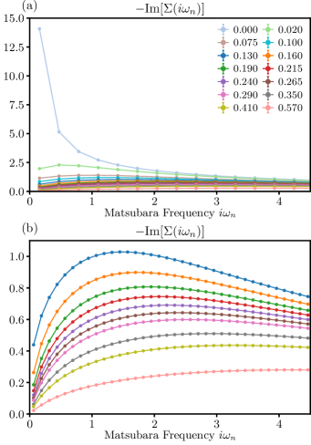
Figure S1: Imaginary component of the electronic self-energy $-\textrm{Im}\Sigma(i\omega_{n})$ vs Matsubara frequency $i\omega_{n}$ at (a) $\beta=20$ and (b) $\beta=50$. At half-filling $\delta=0$, the self-energy diverges at low frequencies $-\textrm{Im}\Sigma(i\omega_{n})\sim 1/i\omega_{n}$, characteristic of the expected insulating behavior (see [27]). At $\beta=50$ and doping values $p=0.130$-$0.190$ close to the critical point, the frequency dependance is more singular than linear close to $i\omega_{n}=0$. This reflects the anomalous scaling discussion in Fig. 3 (main text).

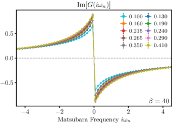
Figure S2: Imaginary component of the electronic Green function $\textrm{Im}G(i\omega_{n})$ vs Matsubara frequency $i\omega_{n}$ at $\beta=40$. All doping values shown ($p>0$) have a discontinuity at $i\omega_{n}=0$, indicative of a metallic states. This is true both for doping in the spin-glass order regime $p\leq p_{c}$ where Luttinger’s theorem breaks down as well as the Fermi liquid regime $p>p_{c}$.

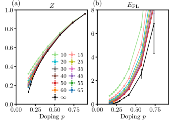
Figure S3: Quasiparticle residue $Z$ and Fermi liquid coherence scale $E_{\mathrm{FL}}$ obtained by fitting $\textrm{Im}\Sigma(i\omega_{n})$ to the Fermi liquid form Eq. (3). For doping values close to the critical point, Fermi liquid theory does not apply, but we can extract $Z,E_{\mathrm{FL}}$ as effective coefficients of the linear and quadratic frequency terms. For $p<p_{c}$ the self-energy has a finite zero-temperature intercept so the form Eq. (3) does not apply.

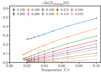
Figure S4: Extrapolated value of the imaginary part of the self-energy. The quantity $-2\textrm{Im}\Sigma_{\mathrm{extrap}}(0)$ is the transport scattering rate. It is interesting to note that it itself is approximately linear in temperature $T$ for doping near $p_{c}$ and low temperatures, which arises from the combination of effective finite temperature dependance of $\alpha,\nu,\lambda$ of Eq. (S11). It is also used in determining the effective single-particle lifetime presented in Fig. 2(c). For $p<p_{c}$, the data extrapolates to a finite value at zero temperature.

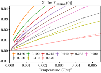
Figure S5: Inverse effective single particle lifetime $-Z\textrm{Im}[\Sigma_{\mathrm{extrap}}(0)]$. This is the same data as plotted in Fig. 2(c), but focused on large values of doping. The system follows the expected $\sim T^{2}$ Fermi liquid behavior (dashed lines) at large $p$ and temperatures below the cross-over scale $T_{\mathrm{FL}}$.

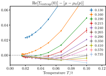
Figure S6: Finite temperature generalization of Luttinger’s invariant $\textrm{Re}\Sigma_{\mathrm{extrap}}(0)-[\mu-\mu_{0}(p)]$; this is the same data as in Fig. 2b shown as a function of temperature $T$. At $p=0.130$, the data extrapolates to a large finite value which shows the transition to a phase distinct from the Fermi liquid at high doping.

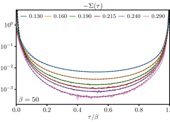
Figure S7: Self-energy in imaginary time $-\Sigma(\tau)$ at low temperature and doping close the QCP. Dashed lines are expressions of the scaling function expected from conformal invariance [Eq. (5) of the main text], with $\alpha,\nu$ taken from fitting the data. This shows that the scaling form holds remarkably well for a large window of $\tau$ close to the long time limit $\tau=\beta/2$.

.7.2 Bosonic Properties

Here we show some additional data related to the spin-spin correlation function $Q$. Figure S8 shows the long time value of $Q$, and shows how solutions with $p<p_{c}$ have tendency towards local moment formations. Figures S9 and S10 are additional plots establishing the critical scaling form of $Q$ at long times.

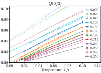
Figure S8: Long-time spin correlation $Q(\beta/2)$. For doping $p<p_{c}$, $Q(\beta/2)$ extrapolates to a finite value at zero temperature, indicating tendency of the paramagnetic solutions to form a local moment at low temperatures (cf. Fig. 4).

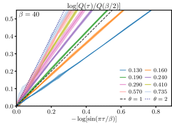
Figure S9: Normalized spin-spin correlation $Q(\tau)/Q(\beta/2)$ at fixed $\beta=40$. This shows the same data as in Fig. 3(c), plotted so that the exponent $\theta$ is the slope of the data at small $-\log|\sin(\pi\tau/\beta)|$. Fermi liquid $\theta=2$ (dotted) and SYK $\theta=1$ (dashed) forms are shown.

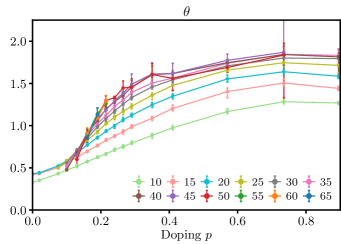
Figure S10: Power of the long-time spin correlation $Q(\tau)$, extracted from scaling plots such as Fig. S9, as a function of doping $p$ and for various $\beta$. This is the same data as is shown in the color-plot background in Fig. 1. The curve $T_{\theta=1}$ of Fig. 1, is obtained by fitting the intersection of the interpolation of the current data with the constant line $\theta=1$; error propagation is done by bootstrap resampling.

References

- Hussey et al. [2003] N. E. Hussey, M. Abdel-Jawad, A. Carrington, A. P. Mackenzie, and L. Balicas, Nature 425, 814 (2003).
- Proust and Taillefer [2019] C. Proust and L. Taillefer, Annu. Rev. Condens. Matter Phys. 10, 409 (2019).
- Doiron-Leyraud et al. [2007] N. Doiron-Leyraud, C. Proust, D. LeBoeuf, J. Levallois, J.-B. Bonnemaison, R. Liang, D. A. Bonn, W. N. Hardy, and L. Taillefer, Nature 447, 565 (2007).
- Fang et al. [2020] Y. Fang, G. Grissonnanche, A. Legros, S. Verret, F. Laliberte, C. Collignon, A. Ataei, M. Dion, J. Zhou, D. Graf, M. J. Lawler, P. Goddard, L. Taillefer, and B. J. Ramshaw, (2020), arXiv:2004.01725 .
- Hussey [2008] N. E. Hussey, J. Phys. Condens. Matter 20, 123201 (2008).
- Taillefer [2010] L. Taillefer, Annu. Rev. Condens. Matter Phys. 1, 51 (2010).
- Varma [2020] C. M. Varma, Rev. Mod. Phys. 92, 031001 (2020).
- Michon et al. [2019] B. Michon, C. Girod, S. Badoux, J. Kačmarčík, Q. Ma, M. Dragomir, H. A. Dabkowska, B. D. Gaulin, J.-S. Zhou, S. Pyon, T. Takayama, H. Takagi, S. Verret, N. Doiron-Leyraud, C. Marcenat, L. Taillefer, and T. Klein, Nature 567, 218 (2019).
- van der Marel et al. [2003] D. van der Marel, H. J. A. Molegraaf, J. Zaanen, Z. Nussinov, F. Carbone, A. Damascelli, H. Eisaki, M. Greven, P. H. Kes, and M. Li, Nature 425, 271 (2003).
- Reber et al. [2019] T. J. Reber, X. Zhou, N. C. Plumb, S. Parham, J. A. Waugh, Y. Cao, Z. Sun, H. Li, Q. Wang, J. S. Wen, Z. J. Xu, G. Gu, Y. Yoshida, H. Eisaki, G. B. Arnold, and D. S. Dessau, Nat. Commun. 10, 5737 (2019).
- Sachdev and Ye [1993] S. Sachdev and J. Ye, Phys. Rev. Lett. 70, 3339 (1993).
- Varma et al. [1989] C. M. Varma, P. B. Littlewood, S. Schmitt-Rink, E. Abrahams, and A. E. Ruckenstein, Phys. Rev. Lett. 63, 1996 (1989).
- Varma [2016] C. M. Varma, Rep. Prog. Phys. 79, 082501 (2016).
- Parcollet and Georges [1999] O. Parcollet and A. Georges, Phys. Rev. B 59, 5341 (1999).
- Florens et al. [2013] S. Florens, P. Mohan, C. Janani, T. Gupta, and R. Narayanan, EPL 103, 17002 (2013).
- Song et al. [2017] X.-Y. Song, C.-M. Jian, and L. Balents, Phys. Rev. Lett. 119, 216601 (2017).
- Chowdhury et al. [2018] D. Chowdhury, Y. Werman, E. Berg, and T. Senthil, Phys. Rev. X 8, 031024 (2018).
- Patel and Sachdev [2019] A. A. Patel and S. Sachdev, Phys. Rev. Lett. 123, 066601 (2019).
- Emery and Kivelson [1995] V. J. Emery and S. A. Kivelson, Phys. Rev. Lett. 74, 3253 (1995).
- Calandra and Gunnarsson [2002] M. Calandra and O. Gunnarsson, Phys. Rev. B 66, 205105 (2002).
- Hussey et al. [2004] N. E. Hussey, K. Takenaka, and H. Takagi, Philos. Mag. 84, 2847 (2004).
- Deng et al. [2013] X. Deng, J. Mravlje, R. Žitko, M. Ferrero, G. Kotliar, and A. Georges, Phys. Rev. Lett. 110, 086401 (2013).
- Hartnoll [2014] S. A. Hartnoll, Nat. Phys. 11, 54 (2014).
- Kitaev [2015] A. Kitaev (2015), talk given at the KITP program: entanglement in Strongly-Correlated Quantum Matter.
- Sachdev [2015] S. Sachdev, Phys. Rev. X 5, 041025 (2015).
- Maldacena and Stanford [2016] J. Maldacena and D. Stanford, Phys. Rev. D 94, 106002 (2016).
- Cha et al. [2020] P. Cha, N. Wentzell, O. Parcollet, A. Georges, and E.-A. Kim, Proc. Natl. Acad. Sci. U.S.A. 117, 18341 (2020).
- Joshi et al. [2020] D. G. Joshi, C. Li, G. Tarnopolsky, A. Georges, and S. Sachdev, Phys. Rev. X 10, 021033 (2020).
- Tikhanovskaya et al. [2021a] M. Tikhanovskaya, H. Guo, S. Sachdev, and G. Tarnopolsky, Phys. Rev. B 103, 075141 (2021a).
- Tikhanovskaya et al. [2021b] M. Tikhanovskaya, H. Guo, S. Sachdev, and G. Tarnopolsky, Phys. Rev. B 103, 075142 (2021b).
- Shackleton et al. [2021] H. Shackleton, A. Wietek, A. Georges, and S. Sachdev, Phys. Rev. Lett. 126, 136602 (2021).
- Bray and Moore [1980] A. J. Bray and M. A. Moore, J. Phys. C: Solid State Phys. 13, L655 (1980).
- Grempel and Rozenberg [1998] D. R. Grempel and M. J. Rozenberg, Phys. Rev. Lett. 80, 389 (1998).
- Arrachea and Rozenberg [2002] L. Arrachea and M. J. Rozenberg, Phys. Rev. B 65, 224430 (2002).
- Otsuki and Vollhardt [2013] J. Otsuki and D. Vollhardt, Phys. Rev. Lett. 110, 196407 (2013).
- Zaanen [2004] J. Zaanen, Nature 430, 512 (2004).
- Homes et al. [2004] C. C. Homes, S. V. Dordevic, M. Strongin, D. A. Bonn, R. Liang, W. N. Hardy, S. Komiya, Y. Ando, G. Yu, N. Kaneko, X. Zhao, M. Greven, D. N. Basov, and T. Timusk, Nature 430, 539 (2004).
- Bruin et al. [2013] J. A. N. Bruin, H. Sakai, R. S. Perry, and A. P. Mackenzie, Science 339, 804 (2013).
- Legros et al. [2019] A. Legros, S. Benhabib, W. Tabis, F. Laliberte, M. Dion, M. Lizaire, B. Vignolle, D. Vignolles, H. Raffy, Z. Z. Li, P. Auban-Senzier, N. Doiron-Leyraud, P. Fournier, D. Colson, L. Taillefer, and C. Proust, Nat. Phys. 15, 142 (2019).
- Grissonnanche et al. [2021] G. Grissonnanche, Y. Fang, A. Legros, S. Verret, F. Laliberté, C. Collignon, J. Zhou, D. Graf, P. A. Goddard, L. Taillefer, and B. J. Ramshaw, Nature 595, 667 (2021).
- Sadovskii [2021] M. V. Sadovskii, Physics-Uspekhi 64, 175 (2021).
- Georges and Mravlje [2021] A. Georges and J. Mravlje, (2021), arXiv:2102.13224 .
- Sengupta and Georges [1995] A. M. Sengupta and A. Georges, Phys. Rev. B 52, 10295 (1995).
- Si and Smith [1996] Q. Si and J. L. Smith, Phys. Rev. Lett. 77, 3391 (1996).
- Smith and Si [2000] J. L. Smith and Q. Si, Phys. Rev. B 61, 5184 (2000).
- Chitra and Kotliar [2000] R. Chitra and G. Kotliar, Phys. Rev. Lett. 84, 3678 (2000).
- Georges et al. [1996] A. Georges, G. Kotliar, W. Krauth, and M. J. Rozenberg, Rev. Mod. Phys. 68, 13 (1996).
- Rubtsov et al. [2005] A. N. Rubtsov, V. V. Savkin, and A. I. Lichtenstein, Phys. Rev. B 72, 035122 (2005).
- [49] See Appendix.
- [50] We perform computations for electron doping ; , where is the electronic density. Due to the model’s symmetry, our results are also true for hole doping, if we change the sign of and particle-hole symmetry odd quantities such as , .
- Chubukov and Maslov [2012] A. V. Chubukov and D. L. Maslov, Phys. Rev. B 86, 155136 (2012).
- Perepelitsky et al. [2016] E. Perepelitsky, A. Galatas, J. Mravlje, R. Žitko, E. Khatami, B. S. Shastry, and A. Georges, Phys. Rev. B 94, 235115 (2016).
- Park et al. [2021] J. M. Park, Y. Cao, K. Watanabe, T. Taniguchi, and P. Jarillo-Herrero, Nature 592, 43 (2021).
- Gourgout et al. [2021] A. Gourgout, G. Grissonnanche, F. Laliberté, A. Ataei, L. Chen, S. Verret, J. S. Zhou, J. Mravlje, A. Georges, N. Doiron-Leyraud, and L. Taillefer, (2021), arXiv:2106.05959 .
- Ghawri et al. [2020] B. Ghawri, P. S. Mahapatra, S. Mandal, A. Jayaraman, M. Garg, K. Watanabe, T. Taniguchi, H. R. Krishnamurthy, M. Jain, S. Banerjee, U. Chandni, and A. Ghosh, (2020), arXiv:2004.12356 .
- Parcollet et al. [1998] O. Parcollet, A. Georges, G. Kotliar, and A. Sengupta, Phys. Rev. B 58, 3794 (1998).
- Sengupta [2000] A. M. Sengupta, Phys. Rev. B 61, 4041 (2000).
- Vojta et al. [2000] M. Vojta, C. Buragohain, and S. Sachdev, Phys. Rev. B 61, 15152 (2000).
- Georges et al. [2000] A. Georges, O. Parcollet, and S. Sachdev, Phys. Rev. Lett. 85, 840 (2000).
- Georges et al. [2001] A. Georges, O. Parcollet, and S. Sachdev, Phys. Rev. B 63, 134406 (2001).
- Frachet et al. [2020] M. Frachet, I. Vinograd, R. Zhou, S. Benhabib, S. Wu, H. Mayaffre, S. Krämer, S. K. Ramakrishna, A. P. Reyes, J. Debray, et al., Nat. Phys. 16, 1064 (2020).
- Cao et al. [2020] Y. Cao, D. Chowdhury, D. Rodan-Legrain, O. Rubies-Bigorda, K. Watanabe, T. Taniguchi, T. Senthil, and P. Jarillo-Herrero, Phys. Rev. Lett. 124, 076801 (2020).
- Parcollet et al. [2015] O. Parcollet, M. Ferrero, T. Ayral, H. Hafermann, I. Krivenko, L. Messio, and P. Seth, Comput. Phys. Commun. 196, 398 (2015).
- [64] N. Wentzell and O. Parcollet, Unpublished .
- Gull et al. [2011] E. Gull, A. J. Millis, A. I. Lichtenstein, A. N. Rubtsov, M. Troyer, and P. Werner, Rev. Mod. Phys. 83, 349 (2011).