Future tests of parton distributions

We discuss a test of the generalization power of the methodology used in the determination of parton distribution functions (PDFs). The “future test” checks whether the uncertainty on PDFs, in regions in which they are not constrained by current data, are compatible with future data. The test is performed by using the current optimized methodology for PDF determination, but with a limited dataset, as available in the past, and by checking whether results are compatible within uncertainty with the result found using a current more extensive dataset. We use the future test to assess the generalization power of the NNPDF4.0 unpolarized PDF and the NNPDFpol1.1 polarized PDF methodology. Specifically, we investigate whether the former would predict the rise of the unpolarized proton structure function $F_{2}$ at small $x$ using only pre-HERA data, and whether the latter would predict the so-called “proton spin crisis” using only pre-EMC data.

Prepared for the 60th anniversary of the Cracow School of Theoretical Physics
to be published in the proceedings

1 Parton distributions in the era of precision

Knowledge of parton distribution functions (PDFs), or lack thereof, is currently one of the dominant sources of uncertainty in the computation of LHC processes. Over the last several years, as the precision of PDF determinations has been gradually improving, a major issue has been that of making sure that this increased precision is matched by a correspondingly high accuracy. Specifically, the question is whether uncertainties due to the methodology used in PDF extraction are estimated accurately. As well known, the problem in determining parton distributions is lack of knowledge of their underlying functional form. Because one is extracting a probability distribution for a set of functions from a discrete set of data points, it is necessary to make assumptions in order to make the problem solvable. The question is then how to reliably estimate the uncertainty coming from these assumptions.

Over the last several years, it has been shown that this problem can be successfully handled using machine learning techniques, by essentially viewing it as a pattern recognition problem (see Ref. [2] for a recent review). The basic idea is that standard tools, such as neural networks, can be used to infer an underlying pattern, i.e. the shape of the PDF, without having to assume a functional form. Redundancy then ensures that no bias is introduced, while quality control tools, such as cross-validation, ensure that the most general result which is compatible with the data is obtained, without also reproducing statistical noise. Uncertainties are obtained as the spread of a population of equally good best-fits. The reader is referred to more detailed discussions [3, 4, 5, 2] for a treatment of this machine-learning based methodology and how it relates to other approaches used for PDF determination.

This paper deals with the issue of validating PDFs, specifically those determined using machine learning methods. As we shall see, this validation problem really consists of two different problems: the first has to do with the ability of machine learning tools to learn an unknown underlying law, and the second has to do with their generalization power. Whereas there are now relatively well-established tools for the validation of the former, here we discuss a new tool for the validation of the latter: the “future test”. We will first discuss in Section 2 the issue of PDF validation. In order to make the discussion self-contained, we briefly review, in Section 2.1, the relation between PDFs and the underlying data, and we then turn, in Section 2.2, to an explanation of the reason why a new validation method is needed, specifically in order to address generalization, and to a presentation of the idea of the future test. In the remaining two sections, we see the future test at work, by applying it to unpolarized (Section 3) and polarized (Section 4) PDFs. Specifically, we discuss the small $x$ rise of the unpolarized structure function $F_{2}$ at HERA, and the “spin crisis”, related to the first measurements of the polarized structure function $g_{1}$. In both cases, we address the issue whether these then-surprising discoveries could have been predicted, had modern-day methodology been available.

2 Validation of PDFs

The original motivation for introducing machine learning tools in PDF determination [6] is to avoid the sources of bias involved in other methodologies, such as the need to pick a particular functional form, or an insufficiently flexible choice of model. The claim that a certain methodology is unbiased, or less biased, however, immediately raises the question: how can we make sure that results, and specifically uncertainties, are faithful? The choice of using machine learning tools suggests that validation should be performed a posteriori, given the lack of direct control on the underlying model. In searching for an a posteriori validation methodology there are then two rather distinct issues, corresponding to the kinematic regions we consider.

2.1 Factorization and kinematic regions

In order to understand the different issues related to PDF validation it is necessary to briefly recall the way PDFs are related to the observable cross sections that are used in order to determine them. Consider specifically a hadronic collision. A typical cross section $\sigma(Q^{2},\tau,\{k\})$ is expressed in terms of PDFs as

$$\sigma(Q^{2},\tau,\{k\})=\sum_{ij}\int_{\tau}^{1}\frac{dz}{z}{\cal L}_{ij}(z,Q^{2})\hat{\sigma}_{ij}\left(\frac{\tau}{z},\alpha_{s}(Q^{2}),\{k\}\right),$$ (1)

where $\hat{\sigma}_{ij}$ is the (“partonic”) cross section for producing the desired final state with incoming partons $i$, $j$, $Q^{2}$ is a hard scale (for example, for $Z$ production, the $Z$ mass $Q^{2}=M^{2}_{Z}$), $\tau$ is a dimensionless scaling variable (for example, for the total inclusive $Z$ production cross section, the ratio $\tau=M_{Z}^{2}/s$, with $s$ the center-of-mass energy), and $\{k\}$ denotes the set of other kinematic variables that the (generally differential) cross section $\sigma$ may depend upon (for example, the rapidity of the dilepton pair into which the $Z$ decays). The dependence on the PDFs is contained in the luminosity

$${\cal L}_{ij}(z,Q^{2})=\int_{x}^{1}\frac{dx}{x}f_{i}^{h_{1}}(x,Q^{2})f_{j}^{h_{2}}\left(\frac{z}{x},Q^{2}\right),$$ (2)

where $f^{h_{k}}_{i}(x,Q^{2})$ is the PDF for extracting a parton of species $i$ from hadron $h_{k}$, carrying a fraction $x$ of its momentum at scale $Q^{2}$.

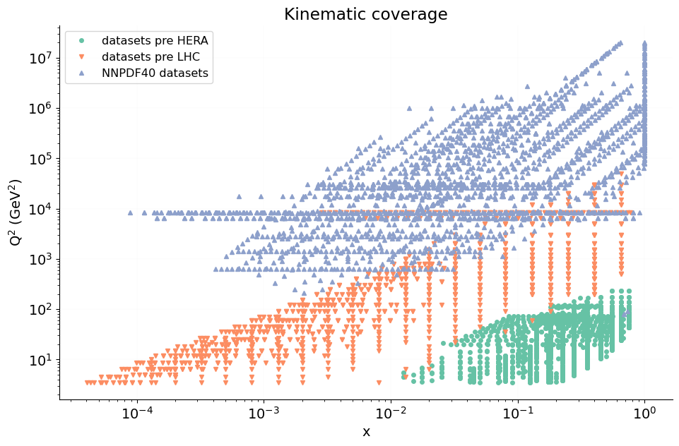
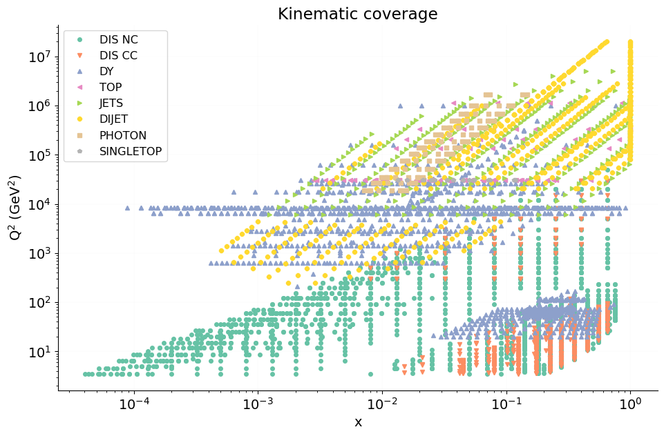
Figure 1: Scatter plot for the datapoints entering the NNPDF4.0 PDF determination and future tests in the unpolarized case, listed in Table 1. The data are shown color-coded by future test grouping (left), and the full dataset is also shown color-coded by physics process (right).

Now, the structure of Eq. (2) trivially implies that only PDFs in a certain range are probed by any given physical process: specifically, the PDF for $x<\tau$ completely decouples from an observable measured at $\tau$. Furthermore, the dominant contribution to any given process typically comes from a restricted kinematic region: in the simplest case, from a single kinematic point. For example, if the $Z$ rapidity distribution is evaluated at leading order, the partonic cross section $\hat{\sigma}$ is proportional to a two-dimensional Dirac delta which removes the convolution integrals from Eq. (2), and only PDFs evaluated for the fixed values $x_{1}=\tau\exp\left(\frac{1}{2}\eta\right)$, $x_{2}=\tau\exp-\left(\frac{1}{2}\eta\right)$, $Q^{2}=M^{2}_{Z}$ contribute, with $\eta$ the rapidity of the $Z$ boson. Even when the kinematics is completely fixed, it is only fixed at leading perturbative order; at higher perturbative orders the cross section is no longer a Dirac delta, and all values of $x$ which are larger than that fixed by leading-order kinematics are accessible, with the smaller $x$ region remaining inaccessible. This is easy to understand physically: at higher perturbative order a parton can always radiate other partons, so all partons that carry a momentum fraction of their parent hadron which is larger than the minimal value needed in order to produce the desired final state can contribute. However, they must at least carry the minimal required momentum fraction. Therefore, for any given process, there is a minimal value of $x$, though in principle no maximal value.

In Fig. 1 we show a scatter plot of data used for a current determination of unpolarized PDFs: each point corresponds to the value of $x$ and $Q^{2}$ at which the PDF contributes to each datapoint, determined using leading-order kinematics, whenever the kinematics of the leading-order process completely fixes them, and the minimum value of $x$, whenever it does not fix them completely (such as for single-inclusive jets). Note that, as already mentioned, the region of $x$ smaller than the smallest $x$ datapoints of Fig. 1 is completely inaccessible. The larger $x$ region is in principle accessible at higher orders, though in practice this is hardly the case for sufficiently large $x$ (say $x\gtrsim 0.5$). Indeed, PDFs vanish at $x=1$ and drop quite fast as $x$ increases (typically as a power of $(1-x)$) so, for many processes, not only the contribution from larger $x$ arises at higher perturbative orders, but also, it rapidly becomes much smaller than that from the smallest value of $x$, thus being in practice unobservable.

Inspection of Fig. 1 immediately shows that the PDF determination, and its validation, entails two rather distinct issues, related to the fact that data points are localized in a well-defined, connected kinematic region — the “data region”, henceforth. On the one hand, the problem of determining PDFs in the region probed by the data remains mathematically ill-posed, because one is determining a function from a piece of discrete information. Yet, because of the convolution integral, PDFs are not probed at a single point, but rather in a region, and also, even in the polarized case, where data are more scarce, datapoints are typically dense in the experimentally accessible kinematic region, because experimental collaborations strive to measure physical observables with as fine a binning as possible. Consequently, whereas lack of knowledge of the PDF functional form entails that a population of equally likely best-fits to any given set of data is possible, assumptions of smoothness, which are physically justified, and built in standard machine-learning interpolants (such as neural networks) ensure that a reasonably narrow set of results follow.

On the other hand, in the small and large $x$ regions which are not probed by the data — the “extrapolation region”, henceforth — the uncertainty is a priori infinite, unless one introduces some assumptions allowing for generalization of the behavior observed in the region covered by the data. Infinite uncertainties would imply the impossibility of predicting any hadronic process, such as Higgs production. Indeed, the bulk of the PDF information which is necessary to predict a given LHC process can be estimated using suitable tools [7], but a certain amount of extrapolation is always needed. The only way to avoid this unpalatable conclusion is to introduce some assumption — motivated by physical considerations, or perhaps based on extrapolating, or generalizing a behavior seen in the data region.

2.2 Validation methods: closure tests and future tests

We can now discuss validation in the data and extrapolation region, and why they differ. The validation of PDF uncertainties in the data region has been addressed in Ref. [8] (see also Refs. [2, 9, 10] for an update): it can be performed using the closure test methodology. The idea is to assume a particular “true” underlying form of the PDFs, generate data based on this assumption, with some statistical distribution corresponding to a particular covariance matrix (typically, the same as that of the true experimental data) and then perform the PDF determination on this data. The faithfulness of the uncertainties can be checked by comparing the distribution of answers when the procedure is repeated several times with the true value, which is now known. Because both the experimental uncertainties and the theory are now completely correct by construction — they are used in the data generation — the procedure tests the accuracy and reliability of the methodology.

The validation of the methodology in the extrapolation region is an open issue: it is the problem that we would like to address here. There is a fundamental reason why this cannot be approached in the same way as the validation in the data region, so in particular a closure test is not advisable. This is related to the fact that the current methodology, if correctly implemented, incorporates the constraints which are present (even if sometimes not explicitly known) in the current data. In order to understand this, consider a simple example. It is known that PDFs satisfy sum rules (see e.g. Ref. [3]) : for example the momentum sum rule

$$\sum_{i}\int_{0}^{1}\,dxxf_{i}(x,Q^{2})=1$$ (3)

where the sum runs over all parton species, which holds for all values of $Q^{2}$. Equation (3) expresses the fact that the total momentum carried by all partons adds up to the momentum of their parent hadron. Because this is a known property of QCD, it is usually imposed as a hard-wired constraint; however it can be checked that if it is not imposed it is actually reproduced by the PDFs extracted from the data [11].

Now, the machine learning methodology for PDF determination is actually optimized on existing data. This optimization was done by trial and error in the past, and it is currently performed, at least in part, using automatic hyperoptimization techniques [12, 2]. Clearly, this optimization is performed in the space of possible solutions, which is a subspace of all possible PDFs, incorporating both known constraints, such as the momentum sum rule Eq. (3), but also possible constraints that we do not know of.

Assume now for the sake of argument that we did not know the momentum sum rule. A methodology optimized on current data would work well on data that respect it. In order to closure-test the methodology we have to assume an underlying functional form. Typically, we would assume that a true PDF is one PDF as determined now, and so even if we did not know the momentum sum rule we would generate data that respect it to good approximation, and use them to closure-test a methodology that unknown to us incorporates this constraint. So the test would be meaningful.

But assume now that we generated data outside the currently measured region. We would then have to make some assumption on the underlying PDF there, and this might not incorporate true constraints that hold there, or it might actually include some constraints that in actual fact do not really hold. In our example, if we did not know the momentum sum rule, we might generate pseudodata that violate it. A validation based on this procedure would then be unreliable because there is no way to know whether there is a mismatch between constraints in the generated data and the methodology. In other words, closure testing is only effective if the generated data carry an amount of information that is smaller, or at most comparable, to real data. If the generated data carry more information— as it must be the case if closure testing the extrapolation region — there is no way to know whether a bias in the methodology will go undetected, or whether the test would force a bias upon the methodology itself.

The idea of the future test is to verify whether a methodology optimized on current data generalizes correctly the features contained in a subset of this data. So, for example, a future test of the methodology used for the NNPDF3.1 determination of PDFs [13] consists of using the same methodology to extract PDFs from, say, only the deep-inelastic scattering (DIS) subset of the NNPDF3.1 dataset. The future test then amounts to comparing these PDFs to the full NNPDF3.1 dataset. Indeed, DIS data cannot constrain the large $x$ gluon PDF, which is instead well determined by LHC data in the NNPDF3.1 dataset [14]. So, if one compares these data to PDFs determined from DIS only, one is testing whether the methodology manages to generalize the gluon PDF outside the data region.

The simplest way to perform the test is to view the computation of all data not included in the PDF fit as a prediction, and compare this prediction, with its PDF uncertainty, with the actual value. The future test is then successful if the $\chi^{2}$ per data point is of order one, because this means that the PDF uncertainties have been estimated faithfully in the extrapolation region. More quantitatively, a criterion for the future test to be successful can be spelled out as

$$|{\chi^{2}}^{\rm PDF}_{\rm not~{}fitted}-\chi^{2}_{\rm fitted}|\ll|{\chi^{2}}^{\rm PDF}_{\rm not~{}fitted}-\chi^{2}_{\rm not~{}fitted}|,$$ (4)

where we denote by ${\chi^{2}}^{\rm PDF}$ and ${\chi^{2}}$ respectively the $\chi^{2}$ per datapoint with and without PDF uncertainties included. In other words, the test is successful if the inclusion of the PDF uncertainties accounts for the missing information which leads the predictions for data which are not fitted to deviate from the measured values.

The test can be thought of as the comparison of a prediction of future data with the future data themselves - hence the name. However, this is a manner of speaking: it is important to understand what the future test does and does not test. The future test does not test whether current data could have been predicted in the past, because the future test tests the current methodology. Indeed, the methodology that we are future testing is optimized to the current dataset: our goal is to test the generalization power of our current best methodology. To this purpose, we test the capability of this methodology of extracting features of the full dataset from a subset, i.e. its generalization power. Also, the future test relies on all the information which is available on the full present-day dataset, both from an experimental and a theoretical point of view. So, for example, we now know that some data must be treated at the highest perturbative accuracy which is currently available, and these data are therefore excluded from PDF determinations which are now performed at a lower perturbative order — but higher order corrections may have been unavailable when these data were originally published.

In this sense, the future test is weaker than a closure test. Indeed, a successful future test is necessary but not sufficient in order to guarantee that the extrapolation of current PDFs outside their data region is reliable. It could be that a reliable extrapolation requires information that is currently inaccessible: however, this is the best we can do now. This is akin to the situation that arises when estimating uncertainties related to missing higher order terms in a perturbative computation. The best we can do is to base the estimate on the known terms, but it cannot be excluded that some new piece of information is needed, which only arises at some higher perturbative order, in which case the estimate is unreliable. Even so, the future test poses stringent requirements on PDFs, as we will show in explicit examples in the next sections.

pre-HERA	Ref.	$N_{\rm{dat}}$
NMC $d/p$	[15]	121
NMC $p$	[16]	204
SLAC $p$	[17]	33
SLAC $d$	[17]	34
BCDMS $p$	[18]	333
BCDMS $d$	[19]	248
CHORUS $\sigma_{CC}^{\nu}$	[20]	416
CHORUS $\sigma_{CC}^{\bar{\nu}}$	[20]	416
NuTeV $\sigma_{c}^{\nu}$	[21]	39
NuTeV $\sigma_{c}^{\bar{\nu}}$	[21]	37
DYE 866 $\sigma^{d}_{\rm DY}/\sigma^{p}_{\rm DY}$	[22]	15
DY E886 $\sigma^{p}_{\rm DY}$	[23]	89
DY E605 $\sigma^{p}_{\rm DY}$	[24]	85
Total pre-HERA		2070
pre-LHC	Ref.	$N_{\rm{dat}}$
HERA I+II inclusive NC $e^{-}p$	[25]	159
HERA I+II inclusive NC $e^{+}p$ 460 GeV	[25]	204
HERA I+II inclusive NC $e^{+}p$ 575 GeV	[25]	254
HERA I+II inclusive NC $e^{+}p$ 820 GeV	[25]	70
HERA I+II inclusive NC $e^{+}p$ 920 GeV	[25]	377
HERA I+II inclusive CC $e^{-}p$	[25]	42
HERA I+II inclusive CC $e^{+}p$	[25]	39
HERA comb. $\sigma_{c\bar{c}}^{\rm red}$	[26]	37
HERA comb. $\sigma_{b\bar{b}}^{\rm red}$	[26]	26
CDF $Z$ rapidity	[27]	28
D0 $Z$ rapidity	[28]	28
D0 $W\to\mu\nu$ asymmetry	[28]	9
Total pre-LHC		1273
NNPDF4.0	Ref.	$N_{\rm{dat}}$
ATLAS $W,Z$ 7 TeV	[29]	30
ATLAS HM DY 7 TeV	[30]	5
ATLAS low-mass DY 7 TeV	[31]	6
ATLAS $W,Z$ 7 TeV central selection	[32]	46
ATLAS $W,Z$ 7 TeV forward selection	[32]	15
ATLAS DY 2D 8 TeV	[33]	48
ATLAS $W,Z$ inclusive 13 TeV	[34]	3
ATLAS $W^{+}$+jet 8 TeV	[35]	16

NNPDF4.0 (cont.’d)	Ref.	$N_{\rm{dat}}$
ATLAS $W^{-}$+jet 8 TeV	[35]	16
ATLAS $Z$ $p_{T}$ 8 TeV $(p_{T}^{ll},M_{ll})$	[36]	44
ATLAS $Z$ $p_{T}$ 8 TeV $(p_{T}^{ll},y_{ll})$	[36]	48
ATLAS $\sigma_{tt}^{\rm tot}$ 7, 8, 13 TeV	[37, 38]	3
ATLAS $t\bar{t}$ $y_{t}$ normalized 8 TeV	[39]	4
ATLAS $t\bar{t}$ $y_{t\bar{t}}$ normalized 8 TeV	[39]	4
ATLAS $t\bar{t}$ normalized $|y_{t}|$ dilepton 8 TeV	[40]	5
ATLAS jets 8 TeV, R=0.6	[41]	171
ATLAS dijets 7 TeV, R=0.6	[42]	90
ATLAS direct photon production 13 TeV	[43]	53
ATLAS single top $R_{t}$ 7 TeV	[44]	1
ATLAS single top $R_{t}$ 13 TeV	[45]	1
ATLAS single top $y_{t}$ norm. 7, 8 TeV	[44, 46]	6
ATLAS single antitop $y$ norm. 7, 8 TeV	[44, 46]	6
CMS $W$ electron asymmetry 7 TeV	[47]	11
CMS $W$ muon asymmetry 7 TeV	[48]	11
CMS Drell-Yan 2D 7 TeV	[49]	110
CMS $W$ rapidity 8 TeV	[50]	22
CMS $Z$ $p_{T}$ $(p_{T}^{ll},y_{ll})$ 8 TeV	[51]	28
CMS dijets 7 TeV	[52]	54
CMS 3D dijets 8 TeV	[53]	122
CMS $\sigma_{tt}^{\rm tot}$ 7, 8, 13 TeV	[54, 55]	3
CMS $t\bar{t}$ rapidity $y_{t\bar{t}}$ $\ell$+jet 8 TeV	[56]	9
CMS $\sigma_{tt}^{\rm tot}$ 5 TeV	[57]	1
CMS $t\bar{t}$ 2D $2\ell$ $(m_{t\bar{t}},y_{t})$ 8 TeV	[58]	16
CMS $t\bar{t}$ absolute $y_{t}$ $\ell$+jet 13 TeV	[59]	10
CMS $t\bar{t}$ absolute $|y_{t}|$ $2\ell$ 13 TeV	[60]	11
CMS single top $\sigma_{t}+\sigma_{\bar{t}}$ 7 TeV	[61]	1
CMS single top $R_{t}$ 8 TeV	[62]	1
CMS single top $R_{t}$ 13 TeV	[63]	1
LHCb $Z$ 940 pb	[64]	9
LHCb $Z\to ee$ 2 fb	[65]	17
LHCb $W,Z\to\mu$ 7 TeV	[66]	29
LHCb $W,Z\to\mu$ 8 TeV	[67]	30
LHCb $Z\to\mu\mu$ 13 TeV	[68]	16
LHCb $Z\to ee$ 13 TeV	[68]	15
Total NNPDF4.0		1148
Grand total		4491

Table 1: The pre-HERA, pre-LHC and NNPDF4.0 datasets: for each experiment the reference to the original publication and the number of datapoints are given. Pre-HERA PDFs are fitted to pre-HERA data, pre-LHC PDFs are fitted to the pre-HERA and pre-LHC data, and NNPDF4.0 PDFs are fitted to the union of the three datasets.

3 Unpolarized PDFs and the rise of structure functions

We start by presenting a future test of the NNPDF4.0 methodology. This is a methodology based, for the first time, on automatic hyperoptimization [12] (see [2] for a review). PDFs constructed with this methodology are currently in a testing phase and will be released soon [9]. This methodology is the state of the art in PDF determination based on machine learning, and it is used for a PDF determination based on a dataset whose size exceeds any previous determination, specifically including a large number of LHC Run II data. Consequently, PDF uncertainties are smaller than in any previous PDF determination, and validation issues are particularly important. The validation of NNPDF4.0 PDFs in the data region, performed using an updated version [2] of the closure test methodology of Ref. [8], will be discussed in Ref. [9].

We choose to use the most recent NNPDF4.0 methodology as a first illustration of the future test because PDF uncertainties found with this methodology are relatively smaller, and thus the issue of accurately estimating PDF uncertainties in extrapolation is particularly serious. However, the methodology that we will discuss in Section 4 in the polarized case is essentially the same as the unpolarized NNPDF3.1 methodology: hence this methodology will also be implicitly future-tested there. A direct comparison between future tests of subsequent NNPDF methodologies is an interesting topic that will be left for future studies [9]. A relevant observation, in this respect, is that all published NNPDF PDF sets turned out to be forward-backward compatible, in the sense that more recent PDFs have smaller uncertainties, but are compatible within uncertainties with previously published ones.

3.1 Gluons and HERA, quarks and the LHC

We performed future tests of the NNPDF4.0 methodology based on two datasets of increasing size: a pre-HERA dataset, which only includes fixed-target DIS and Drell-Yan production data; and a dataset obtained by combining this with a pre-LHC dataset, which also includes HERA DIS data and Tevatron collider $W$, $Z$ production and single-inclusive jet data. The NNPDF4.0 PDFs are determined by adding to these also an NNPDF4.0 dataset, which includes LHC data for $W$ and $Z$ production, single-inclusive jets and dijets, $Z$ transverse momentum distributions, single top and top pair production, and prompt photon production. Note that PDFs are thus determined from strictly hierarchical datasets: pre-HERA PDFs are determined from the pre-HERA data, pre-LHC PDFs are determined combining pre-HERA and pre-LHC data, and NNPDF4.0 PDFs are determined combining pre-HERA, pre-LHC, and NNPDF4.0 data. Although, as explained in Section 2.2 the historical nature of these datasets is somewhat besides the point, since the future test is a test of current PDF methodology, it might be useful to think about these datasets roughly as those on which PDF determinations were respectively based circa 1993, such as the CTEQ1 [69] or MRS [70] PDFs, for the pre-HERA PDFs, and circa 2010, such as NNPDF2.1 [71] for the pre-LHC PDFs.

The three datasets are listed in Table 1 and displayed in Fig. 1, where the breakdown of the full dataset into single processes is also shown. The choice of these two future test datasets is motivated by aspects having to do both with physics and methodology. In terms of physics, the pre-LHC dataset only imposes very weak constraints on the flavor separation of quarks and antiquarks, and also on the large-$x$ gluon. In the pre-LHC dataset, the small $x$ gluon is also unconstrained, so in fact the gluon is largely unconstrained, except in a very small region around $x\sim 0.1$. In terms of methodology, a pre-LHC fit tests whether relatively small PDF uncertainties (of order of say 5-10%) are compatible with later more precise data: i.e., it tests the ability of the methodology to perform a near extrapolation. On the contrary, the pre-HERA fit tests whether the methodology can capture broad features of the results even in the presence of a minimal amount of information: i.e. it tests the far extrapolation.

A particularly intriguing aspect of the pre-HERA future test in this respect is the small $x$ behavior of the gluon PDF, and correspondingly of the $F_{2}$ proton structure function. Indeed, when this structure function was first measured at HERA the observed rise of the structure function at small $x$ (see e.g. [72]) came as a surprise, and indeed standard pre-HERA PDF sets displayed a wide variety of small-$x$ gluon behaviors, with a flat gluon taken as a baseline option in the absence of new physics effects [70]. A rather steeper rise of the gluon at small $x$ is a common feature of all post-HERA PDF sets (see [73] for a comparative discussion). It is thus interesting to wonder how a contemporary methodology, presented with pre-HERA data, would behave in this respect.

3.2 Future testing NNPDF4.0

	$n_{\rm dat}$	NNPDF4.0	pre-LHC	pre-HERA	NNPDF4.0	pre-HERA	pre-LHC
pre-HERA dataset	2070	1.09	1.01	0.90	(1.02)	(0.95)	(0.86)
pre-LHC dataset	1273	1.21	1.20	23.1	(1.18)	(1.17)	1.22
NNPDF4.0 dataset	1148	1.29	3.30	23.1	(1.23)	1.30	1.38
Total dataset	4491	1.17	1.65	12.9	1.12	1.10	1.10

Table 2: The $\chi^{2}$ per datapoint for the NNPDF4.0 PDF determination and its pre-HERA and pre-LHC future tests. Values are shown for the three datasets displayed in Fig. 1. In the left table all values are computed using only the experimental covariance matrix, while in the right table all values are computed by also including PDF uncertainties. Values with PDF uncertainties included computed for data included in the fit, shown in parenthesis, do not have a strict statistical meaning (see text). All numbers in italic (without PDF uncertainty included) and in boldface (with PDF uncertainty included) are predictions.

We now turn to the results of the future test of the NNPDF4.0 methodology. The reader is referred to the forthcoming Ref. [9] for full details on the NNPDF4.0 PDF determination theory and methodology; here, we provide some basic information. The machine-learning methodology which is being future-tested has been constructed through a hyperoptimization procedure [12] and its general features are reviewed in Ref. [2]. It uses the same approach, based on a Monte Carlo representation of PDF uncertainties, and neural networks as underlying interpolants as previous NNPDF determinations, such as the most recent published NNPDF3.1 [13]. It differs from the previous NNPDF methodology in the architecture of neural networks and minimization algorithm, and more importantly, due to the fact that architecture and algorithms have been selected through a hyperoptimization procedure tuned using $K$-foldings, see [2]. Preprocessing is treated according to the most recent NNPDF methodology [74].

The figure of merit which is being minimized is the same as in previous NNPDF determinations, and specifically it includes all available information on statistical and systematic experimental uncertainties and their correlations, through the $t_{0}$ method [75, 76]. NNLO QCD theory is used throughout, with charm quark mass effects included through the FONLL method [77] and a parametrized charm PDF [78, 79]. Uncertainties due to deuterium and heavier nuclear targets are included [80, 81, 82] as a theory uncertainty contribution to the covariance matrix [83].

An identical methodology is used to perform the future tests. The NNPDF methodology calls for the $t_{0}$ covariance matrix [75] and the preprocessing exponents to be determined iteratively and self-consistently: this has been done for each of the two future tests. Results are collected in Table 2, where we show $\chi^{2}$ values for the three PDF sets: namely, the baseline NNPDF4.0, the pre-HERA and the pre-LHC future tests. Values are shown for all data, both included and not included in each fit. We show both standard $\chi^{2}$ values computed using the experimental covariance matrix, and values computed also including PDF uncertainties. Note that the experimental covariance matrix is not the same as the $t_{0}$ covariance matrix used for minimization in order to obtain unbiased results, but just the standard covariance matrix as published by experimental collaborations (see Ref. [76] for a comparative discussion). The $\chi^{2}$ computed using it measures the goodness of fit provided by the PDFs fitted to data.

In the $\chi^{2}$ including PDF uncertainties, these are accounted for by adding to the experimental covariance matrix the PDF uncertainty covariance matrix, in turn computed as the covariance over the NNPDF replica set [84]. The total covariance matrix is then inverted and used in the standard definition of the $\chi^{2}$. Addition of two contributions to the covariance matrix is justified if they correspond to uncorrelated uncertainties [83]. This is surely the case when considering the PDF uncertainty and the uncertainty on new data not used for the determination of those PDF. Consequently, the $\chi^{2}$ values shown in Table 2 with PDF uncertainties included, for the future test PDFs when compared to data not used to fit, indicate whether the PDF uncertainty estimate on these future test PDFs is reliable: it tests the generalization power of the methodology.

Note that, of course, the PDF uncertainty is not uncorrelated to the uncertainty on data used for the determination of the same PDFs, since the latter propagates into the former. Consequently $\chi^{2}$ values computed including PDF uncertainties for datasets included in any PDF determination, shown in parenthesis in Table 2, are only indicative and do not have a strict statistical meaning.

It is important to stress that both the experimental covariance matrix, and the PDF covariance matrix, consistently include correlations. In fact, these are often quite large, and $\chi^{2}$ values found not including correlations would be substantially different. For the experimental covariance matrix, this is because for many LHC data uncorrelated statistical uncertainties are very small: sometimes, for example for $Z$ production data, at the per mille level. Dominant uncertainties are then systematic, and these are typically highly or fully correlated: an example is the luminosity uncertainty, which is common to all data in a given experiment. For the PDF covariance matrix this is due to the fact that many data points are kinematically very close to each other, and of course PDF values and uncertainties on neighboring values of $x$ and $Q^{2}$ are highly correlated.

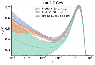
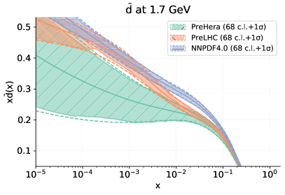
Figure 2: Comparison of the pre-HERA, pre-LHC and NNPDF4.0 PDFs. The up (top left), antidown (top right), strange (bottom left) and gluon (bottom right) PDFs are shown at the parametrization scale $Q=1.7$ GeV.

The relevant information from Table 2 is contained in the $\chi^{2}$ values corresponding to predictions, i.e. computed from data not included in the determination of the corresponding PDF sets. These are shown in italic (without PDF uncertainties) and boldface (with PDF uncertainties). These values show that the future test is impressively successful, and the criterion Eq. (4) is clearly satisfied. Before inclusion of PDF uncertainties (values in italic), the $\chi^{2}$ of future test PDFs is of order 20, but after their inclusion (values in boldface) it becomes of order one, and in fact almost identical to that of fitted PDFs (without uncertainties included). This means that PDF uncertainties increase on average by more than two orders of magnitude in the extrapolation region, and that this increase is exactly of the size required in order to account for the missing information contained in the excluded data. This is especially remarkable for the $\chi^{2}$ of the pre-HERA PDFs when compared to the post-HERA dataset, whose value is hardly larger than that found in the NNPDF4.0 fit itself. In fact, inspection of $\chi^{2}$ values for individual experiments [9] shows that the $\chi^{2}$ values after inclusion of PDF uncertainties are all very close to the values found in the NNPDF4.0 fit (without PDF uncertainties), while, especially for the pre-HERA PDFs, some of the values found withiut PDF uncertainties, especially for experiments in far extrapolation regions, can be up to two orders of magnitude higher, as we will discuss below for some specific examples. This means that uncertainties are quite reliable even in far extrapolation regions.

Note that the $\chi^{2}$ values for the data included in the fit (which, as mentioned, do not have a statistical meaning strictly) are almost unchanged when PDF uncertainties are included. This is due to the fact that, for data included in the fit, the PDF uncertainty is generally rather smaller than that of data used for its determination, because PDFs combine the information coming from many datapoints. Hence for these data the experimental uncertainty is dominant, and this explains why $\chi^{2}$ values are almost unaffected by the inclusion of PDF uncertainties.

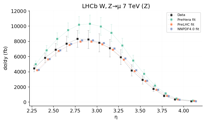
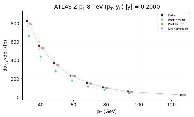
Figure 3: Comparison to experimental data of predictions obtained using the pre-HERA, pre-LHC and NNPDF4.0 PDF sets. The diagonal PDF uncertainties and data uncertainties are shown. Illustrative results are displayed for the HERA $F_{2}$ proton structure function [25] (top left) the CMS double differential top pair distribution [58] (top right), the LHCb $Z$ rapidity distribution [85] (bottom left) and the ATLAS $Z$ $p_{T}$ distribution [36] (bottom right).

A more detailed picture can be obtained by looking at individual PDFs. Specifically, in Fig. 2 the up, antidown, strange quark and gluon PDFs found in the two future test fits are compared to NNPDF4.0. It is clear that PDFs are generally compatible within errors, with differences exceeding the one sigma level in a limited set of cases (as expected given that one sigma corresponds to a $68\%$ confidence level). This is true both for PDFs determined relatively accurately (such as the up quark in the pre-LHC fit), or those affected by large uncertainties (such as the gluon in the pre-HERA fit).

The case of the pre-HERA gluon is especially remarkable: despite the very large uncertainty, the future test correctly extrapolates the small $x$ rising trend. In fact, with hindsight this trend can be seen in some pre-HERA DIS data (especially from NMC), though historically it was overlooked. Of course, the methodology that we are future testing has been hyperoptimized on a dataset that does contain small-$x$ data, so the pre-HERA future test cannot be taken as evidence that the rise of the structure function could have been predicted without the HERA data. However, it does suggest that an unbiased inspection of this data should have at least have suggested this possibility.

In Fig. 3 we also show the comparison of predictions obtained using either NNPDF4.0, or the two future test PDF sets, to data for some physical observables: the HERA $F_{2}$ structure function [25], the CMS double-differential distribution of top pairs [58], the LHCb $W/Z$ rapidity distribution [85] and the ATLAS $Z$ $p_{T}$ distribution [36]. These observables are sensitive to a wide array of PDF features which are poorly constrained by pre-HERA data. Specifically, the HERA structure function probes the small $x$ gluon, the top pair and $Z$ $p_{T}$ distributions depend on the large $x$ gluon and the LHCb large-rapidity $W$ and $Z$ cross sections probe the flavor separation at large $x$. In each case we clearly see hat the PDF uncertainty on the prediction using future test PDF correctly accounts for the deviation from the data, despite the very substantial amount of extrapolation which is required in all cases shown. This is manifestly seen when inspecting the corrresponding $\chi^{2}$ values. For instance, the $\chi^{2}$ values per datapoint for the pre-HERA fit are, for the HERA I+II inclusive NC $e^{+}p$ 920 GeV data, $\chi^{2}=44.2$ without PDF uncertainties and ${\chi^{2}}^{\rm PDF}=1.29$ when PDF uncertainties are included (fitted NNPDF4.0 value $\chi^{2}=1.31$); for CMS $t\bar{t}$ 2D $2\ell$ $(m_{t\bar{t}},y_{t})$ 8 TeV, they are respectively $\chi^{2}=5.125$ and ${\chi^{2}}^{\rm PDF}=1.15$ (fitted NNPDF4.0 value $\chi^{2}=0.89$); for LHCb $W,Z\to\mu$ 7 TeV, $\chi^{2}=15.37$ and ${\chi^{2}}^{\rm PDF}=1.71$ (fitted NNPDF4.0 value $\chi^{2}=1.96$); and for ATLAS $Z$ $p_{T}$ 8 TeV $(p_{T}^{ll},y_{ll})$, $\chi^{2}=28.69$ and ${\chi^{2}}^{\rm PDF}=0.997$ (fitted NNPDF4.0 value $\chi^{2}=0.89$). In all cases, the inclusion of the PDF uncertainties brings down the $\chi^{2}$ to a value that is close to that found when the data are fitted, and the criterion Eq. (4) is very well satisfied, as the figures show graphically.

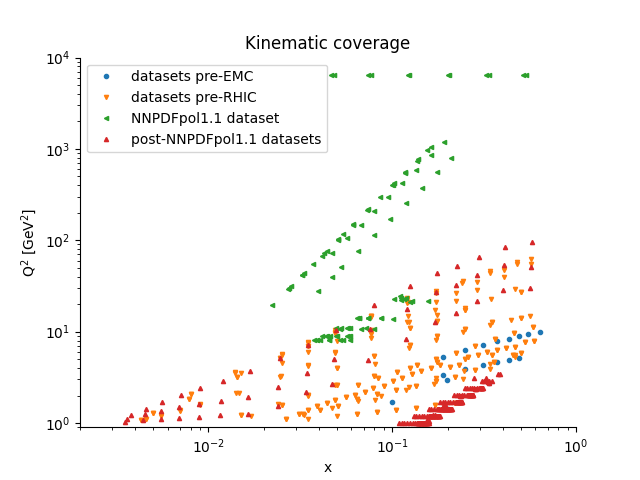
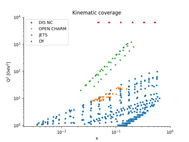
Figure 4: Same as Fig. 1 but now for polarized PDFs.

4 Polarized PDFs and the “spin crisis”

We now turn to longitudinally polarized parton distributions (polarized PDFs, henceforth), defined as

$$\Delta f_{i}(x,Q^{2})=f^{\uparrow\uparrow}_{i}(x,Q^{2})-f^{\uparrow\downarrow}_{i}(x,Q^{2}),$$ (5)

where $f^{\uparrow\uparrow}_{i}$ ($f^{\uparrow\downarrow}$) is the $i$-th species of PDF when the parton’s spin is parallel (antiparallel) to that of its parent hadron, so that unpolarized PDFs are $f_{i}(x,Q^{2})=f^{\uparrow\uparrow}_{i}(x,Q^{2})+f^{\uparrow\downarrow}_{i}(x,Q^{2})$.

Polarized PDFs are based on rather more scarce experimental information than their unpolarized counterparts. Not only a much smaller number of data and processes is available, but also these are typically affected by significantly larger uncertainties. Furthermore fully correlated systematics are often not available, so statistical and systematic uncertainties must be added in quadrature, thereby leading to even larger uncertainties. Extrapolation problems are accordingly more serious for polarized PDFs.

pre-EMC	Ref.	$N_{\rm{dat}}$
SLAC (1978) $A_{1}^{p}$	[86]	4
SLAC (1983) $A_{1}^{p}$	[87]	14
Total pre-EMC		18
pre-RHIC	Ref.	$N_{\rm{dat}}$
EMC $A_{1}^{p}$	[88]	10
SMC $A_{1}^{p}$	[89]	12
SMC $A_{1}^{d}$	[89]	12
SMC (low-$x$) $A_{1}^{p}$	[90]	8
SMC (low-$x$) $A_{1}^{d}$	[90]	8
E143 $A_{1}^{p}$	[91]	25
E143 $A_{1}^{d}$	[91]	25
E154 $A_{1}^{n}$	[92]	11
E155 $g_{1}^{p}$	[93]	20
E155 $g_{1}^{d}$	[93]	20
COMPASS (2007) $A_{1}^{d}$	[94]	15
COMPASS (2010) $A_{1}^{p}$	[95]	15
HERMES (1997) $A_{1}^{n}$	[96]	8
HERMES $A_{1}^{p}$	[97]	28
HERMES $A_{1}^{d}$	[97]	28
Total pre-RHIC		245

NNPDFpol1.1	Ref.	$N_{\rm dat}$
COMPASS open charm $A_{LL}$	[98]	45
STAR 1-jet (2005) $A_{LL}$	[99]	10
STAR 1-jet (2006) $A_{LL}$	[99]	9
STAR 1-jet (2009) $A_{LL}$	[100]	22
PHENIX 1-jet $A_{LL}$	[101]	6
Total NNPDFpol1.1		92
post-NNPDFpol1.1	Ref.	$N_{\rm{dat}}$
COMPASS (2015) $A_{1}^{p}$	[102]	51
COMPASS (2016) $A_{1}^{d}$	[103]	43
JLAB-EG1-DVCS $g_{1}^{p}$	[104]	9
JLAB-EG1-DVCS $g_{1}^{d}$	[104]	9
JLAB-E93-009 $A_{1}^{p}$	[105]	62
JLAB-E93-009 $A_{1}^{d}$	[105]	86
JLAB-E06-014 $A_{1}^{n}$	[106]	2
STAR 2-jet (2009) $A_{LL}$	[107]	14
STAR 1-jet (2012) $A_{LL}$	[108]	14
STAR 2-jet (2012) $A_{LL}$	[108]	42
Total postNNPDFpol1.1		332
Grand Total		687

Table 3: The pre-EMC, pre-RHIC, NNPDFpol1.0 and post-NNPDFpol1.1 datasets: for each experiment the reference to the original publication and the number of datapoints is given. Pre-EMC polarized PDFs are fitted to pre-NMC, pre-RHIC PDFS are fitted to the pre-EMC and pre-RHIC data, and NNPDFpol1.1 PDFs are fitted to the union of these three datasets. Post-NNPDFpol1.1 PDFs are only used for future testing.

4.1 Polarized PDFs and data

Until quite recently, polarized PDFs where determined purely using neutral-current deep-inelastic scattering on proton, deuteron and neutron (i.e., Helium) targets, from the polarized structure function $g_{1}$ directly, or the polarized asymmetries from which the structure function is extracted (see [109] for a review). More recently these were supplemented by open charm and semi-inclusive hadron production and, more importantly, by precious little data on $W$, inclusive jet and pion production from RHIC, see [5] and references therein. The dataset for the most recent determination of polarized PDFs based on the NNPDF methodology, NNPDFpol1.1 [110], is shown in Fig. 4. We have performed a three-fold future test of this PDF set and methodology, by comparing it to pre-EMC and pre-RHIC datasets, and also to a post-NNPDF1.1 dataset. This dataset includes some more recent data, which appeared after the original NNPDFpol1.1 PDF determination. Some of these data were discussed, in the context of NNPDF fits, in Refs. [111, 112] without leading to a fully updated PDF release. The datasets are all shown in Fig. 4, and also listed in Table 3. Because the NNPDFpol1.1 methodology is essentially the same as the NNPDF3.1 methodology, the future tests presented here also effectively test the NNPDF3.1 methodology.

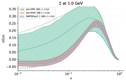
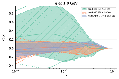
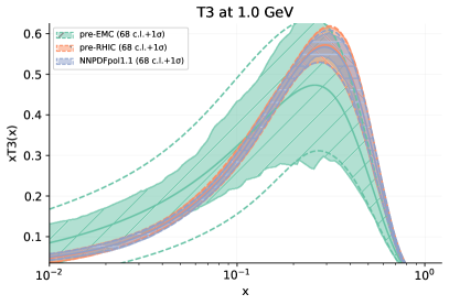
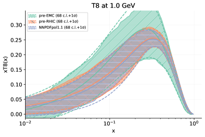
Figure 5: Comparison of the pre-EMC, pre-RHIC and NNPDFpol1.1 PDFs. The singlet (top left), gluon (top right), triplet (bottom left) and octet (bottom right) PDF combinations (see text) are shown at the parametrization scale $Q=1$ GeV.

A PDF determination based purely on neutral-current DIS cannot disentangle quark and antiquark PDFs, and only allows for a determination of their sum:

$$\Delta q_{i}^{+}(x,Q^{2})=\Delta q_{i}(x,Q^{2})+\bar{q}_{i}(x,Q^{2})$$ (6)

for each flavor $i$. Furthermore, DIS on proton targets only determines a fixed linear combination of quark flavors, i.e., in practice a fixed linear combination of up, down and strange contributions since the contribution of heavy quarks is negligible, at least within present-day accuracy. If also deuteron or neutron targets are available, it is then possible to determine separately the triplet combination

$$\Delta T_{3}(x,Q^{2})=\Delta u^{+}(x,Q^{2})-\Delta d^{+}(x,Q^{2})\,.$$ (7)

However, it is not a priori possible to disentangle the two linear combinations orthogonal to it, namely the singlet

$$\Delta\Sigma(x,Q^{2})=\Delta u^{+}(x,Q^{2})+\Delta d^{+}(x,Q^{2})+\Delta s^{+}(x,Q^{2})$$ (8)

and octet

$$\Delta T_{8}(x,Q^{2})=\Delta u^{+}(x,Q^{2})+\Delta d^{+}(x,Q^{2})-2\Delta s^{+}(x,Q^{2})\,.$$ (9)

However, the first moments (i.e. integrals) of triplet and octet can be extracted from weak decays. If only DIS on proton targets is used, this is then the only information available on flavor separation.

The pre-EMC dataset, which only includes proton DIS data, only allows for a determination of quark and gluon (the latter from the $Q^{2}$ dependence), with minimal information on flavor separation from first moments. The pre-RHIC dataset, including proton, deuteron and neutron DIS data allows for a more detailed flavor separation, and a reasonable determination of the triplet. The NNPDFpol1.1 allows for a determination of individual flavor and antiflavors (from $W$ production) with jet production providing a direct handle on the gluon. These datasets are therefore hierarchical in terms of the flavor separation they allow: pre-EMC and pre-RHIC correspond respectively to far and near extrapolation in flavor space.

Figure 6: Comparison to experimental data of predictions obtained using the pre-EMC, pre-RHIC and NNPDFpol1.1 PDF sets. The diagonal PDF uncertainties and data uncertainties are shown. Illustrative results are displayed for the proton structure function $g_{1}^{p}$ measured at SLAC pre-EMC (top left) [87] and measured by SMC (top right) [89], as well as for the E154 measurement of the neutron structure function $g_{1}^{n}$ (bottom left) [92] and the HERMES measurement of the deuterium structure function $g_{1}^{d}$ (bottom right) [97].

As is apparent from Fig. 4, these datasets are also hierarchical in terms of coverage in $(x,Q^{2})$ space. More coverage in $Q^{2}$ allows for a better extraction of the gluon, which is determined mainly by the scale dependence, while more coverage in $x$ allows for a better determination of the first moment of individual PDFs, and in particular the first moment of the singlet combination. Unlike the triplet and octet, the singlet is not determined by weak decays, and has a simple physical interpretation as the fraction of the parent hadron’s spin carried by quarks (up to field theoretical complications related to the axial anomaly [113]). So also in terms of $x$-coverage, gluon determination, and determination of the first moments, the pre-EMC and pre-RHIC datasets correspond to far and near extrapolation.

In fact, this is the reason why specifically a pre-EMC dataset was chosen for future testing. Indeed, when the EMC data [88] were originally published, a first determination of the singlet first moment was possible. The result turned out to be surprising: the first moment was found to be rather smaller than expected, and in fact compatible with zero within uncertainties — which would mean (at least naively) that the proton spin is not carried by quarks. This has been often referred to as the “proton spin crisis” [114]. Hence, just like in the case of the rise of the structure function at HERA, it is natural to wonder what a contemporary polarized methodology would make of pre-EMC data.

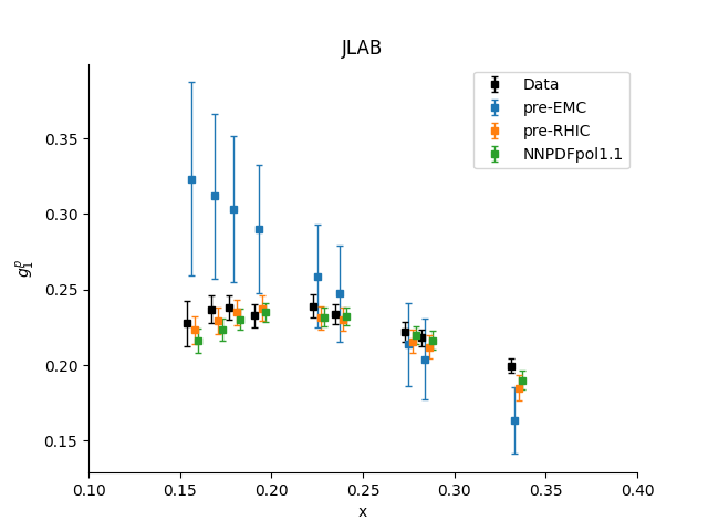
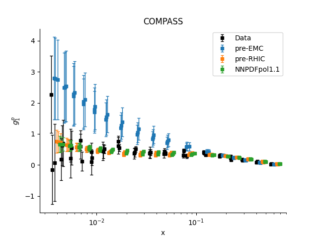
Figure 7: Same as Fig. 6, but now comparing to post-NNPDFpol1.1 data. Results are shown for $g_{1}^{p}$ measured at JLAB (left) [104] and COMPASS (right) [102].

Finally, we have also performed a future test with post-NNPDFpol1.1 data because these significantly extend the precision and also somewhat enlarge the kinematic range of the NNPDFpol1.1 dataset: in a sense these are the first polarized data that provide a first step towards the direction of precision polarized PDFs. However, we have future-tested them using the NNPDFpol1.1 methodology because this is the most recent polarized methodology that we have. In this sense, this future test confirms (or disproves) that the NNPDFpol1.1 methodology is still adequate, even in view of this more recent data.

	$n_{\rm dat}$	NNPDFpol1.1	pre-RHIC	pre-EMC	NNPDFpol1.1	pre-RHIC	pre-EMC
pre-EMC dataset	18	0.53	0.53	1.09	(0.53)	(0.52)	(0.77)
pre-RHIC dataset	245	0.75	0.77	20.4	(0.64)	(0.67)	0.51
NNPDFpol1.1 dataset	92	1.37	1.66	7.36	(1.35)	1.38	1.40
post-NNPDFpol1.1 dataset	332	2.58	2.54	8.46	0.97	0.96	0.90
Total dataset	687	1.54	1.58	13.2	(0.88)	(0.89)	(0.81)

Table 4: The $\chi^{2}$ per datapoint for the NNPDFpol1.0 PDF determination and its pre-EMC and pre-RHIC future tests. Values are shown for the four datasets displayed in Fig. 4. In the left table all values are computed using only the experimental covariance matrix, while in the right table all values are computed by also including PDF uncertainties. Values with PDF uncertainties included computed for data included in the fit, shown in parenthesis, do not have a strict statistical meaning (see text). All numbers in italic (without PDF uncertainty included) and in boldface (with PDF uncertainty included) are predictions.

4.2 Future testing polarized PDFs

The polarized future test tests the NNPDFpol1.1 methodology [110]. This is quite similar to the methodology used for unpolarized NNPDF sets until the most recent published NNPDF3.1 [13]. It differs from the methodology whose future test was discussed in Section 3.2, essentially because it is not obtained from an automatic hyperoptimization procedure, so methodological details, such as the choice of neural network architecture, are based on previous experience rather then being optimized automatically. A peculiar aspect of the polarized fitting methodology is the need to assume an underlying set of unpolarized PDFs, since experimental data are usually presented for polarized asymmetries. Polarized PDF determinations presented in this section assume the published NNPDF3.1 as an underlying unpolarized set.

As in the unpolarized case, we have computed $\chi^{2}$ values for all datasets and PDF sets, both with and without PDF uncertainties included. Results are collected in Table 4. An important caveat in the polarized case is that correlated systematic uncertainties are mostly not available, except for the most recent experiments. Hence, statistical and systematic uncertainties have to be added in quadrature, and the covariance matrix must be taken to be diagonal. We will come back to this point shortly. PDF uncertainties, on the other hand, are always included with all correlations fully accounted for.

As in the unpolarized case, the relevant comparison is between $\chi^{2}$ values for data not included in the fit, before (in italic) and after (in boldface) the inclusion of PDF uncertainties. As in the unpolarized case, we find that all $\chi^{2}$ values with PDF uncertainties included are of order one, thus showing that the future test is successful. The pre-EMC case is especially remarkable, with a $\chi^{2}$ value that, for data not used for fitting, is of order thirteen per datapoint, and decreases to a value of order one once the PDF uncertainty is included. This shows that with only pre-EMC data fitted, uncertainties increase by one and a half order of magnitude, and the increase is exactly the right size to account for the missing information, i.e. the deviation of results from the true value.

When comparing NNPDFpol1.1 data to the pre-RHIC PDFs, and post-NNPDFpol1.1 data to NNPDF1.1pol PDFs, $\chi^{2}$ values are of order three-four per datapoint, which means that the increase of uncertainties in the region of the data not included is not so dramatic, though still noticeable. The data not included only provide a relatively minor extension of kinematic reach, without adding any new process or target. Also in these cases, the $\chi^{2}$ value after inclusion of PDF uncertainties decreases to a value around one, thus showing that uncertainties are correctly estimated also in near extrapolation.

	NNPDpol1.1	pre-EMC	pre-RHIC
$\Delta\Sigma$	$0.18\pm 0.21$	$0.83\pm 0.74$	$0.16\pm 0.30$
$\Delta g$	$0.02\pm 3.24$	$1.71\pm 4.80$	$0.95\pm 3.87$

Table 5: The first moment of the polarized quark singlet and gluon distributions, computed using the NNPDFpol PDF sets and the two future test pre-EMC and pre-RHIC PDF sets, evaluated at the scale $Q^{2}=1$ GeV².

Inspection of the results of Table 4 shows that $\chi^{2}$ values without PDF uncertainties, for datasets which are fitted, is in most cases smaller, and often rather smaller than one. This is due to fact that, as already mentioned, statistical and systematic experimental uncertainties are added in quadrature, because of lack of information on their correlation. This leads to an overestimate of the experimental uncertainties, and thus to an underestimate of the $\chi^{2}$. Also, as mentioned, correlations between PDF uncertainties instead are always consistently included, so when a dataset is not fitted and PDF uncertainties are dominant the expected correct result has a $\chi^{2}$ of order one per datapoint, even if the $\chi^{2}$ of the same dataset when fitted is much smaller than one. The results shown in Table 4 confirm this expectation.

We now turn to a comparison of PDFs. Because, as mentioned, only the three combinations Eqs. (7-9) of PDFs are accessible, it is more convenient to look directly at these, and the gluon. They are compared in Figure 5 for the pre-EMC, pre-RHIC PDF and NNPDFpol1.1 sets. The pre-EMC PDFs are perfectly compatible with NNPDFpol1.1, within their extremely large uncertainties. The pre-RHIC and NNPDFpol1.1 polarized quarks are almost identical, while the pre-RHIC polarized gluon is somewhat more uncertain than the NNPDFpol1.1 gluon, especially at large $x\gtrsim 0.1$, but in very good agreement with it.

As discussed in Section 4.1 much of the interest in polarized PDFs is related to the EMC discovery that the first moment of the polarized quark distribution is unusually small, and in fact compatible with zero within uncertainties. This also raised interest in the value of the first moment of the polarized gluon distribution, both because of its possible role in carrying a sizable fraction of the proton spin, and also, in explaining the smallness of the quark first moment at low scale due to its mixing with it driven by the axial anomaly [113]. Note that, as mentioned, the first moment of the triplet and octet combinations Eqs. (7-9) are instead fixed by weak meson decay constants.

The values of the polarized quark singlet and gluon first moments are collected in Table 5 for the NNPDFpol1.1, pre-EMC and pre-RHIC polarized PDF sets. Of course, the qualitative behavior of the first moments is the same as that of the PDFs seen in Figure 5: they are all compatible within uncertainties, with pre-EMC uncertainties much larger, and pre-RHIC uncertainties somewhat larger for the quark and rather larger for the gluon in comparison to NNPDFpol1.1. The “spin crisis”, with the polarized singlet quark first moment compatible with zero, and significantly different from a value of order one, is clearly seen already in the pre-RHIC PDF set. On the other hand, no conclusion on the polarized quark first moment can be drawn from pre-EMC data: the result is compatible both with zero and with one, within its large uncertainty. Even with contemporary fitting methodology, no hint of the “spin crisis” can be seen in pre-EMC data. The spin crisis was a real experimental surprise. Interestingly, knowledge of the gluon first moment has not improved much over the years: both a vanishing value, or a large value (a possible explanation of the “spin crisis”) are compatible with both EMC and contemporary data.

Finally, in Figure 6 we compare predictions for selected pre-EMC and pre-RHIC data, and in Figure 7 for selected post-NNPDFpol1.1 data, obtained using the three polarized PDF sets. The excellent compatibility of the three PDF sets with each other and with all the NNPDFpol1.1 data is clear, with the uncertainties of the pre-EMC PDFs very large, and of the right amount to account for the missing information from the subsequent data. The post-NNPDFpol1.1 data pose more stringent requirements on the NNPDFpol1.1 PDFs, whose uncertainties are just large enough to accommodate them, as we had seen already from the $\chi^{2}$ values of Table 4. It is apparent from these plots how the PDF uncertainty correctly accounts for the deviation between data, and predictions obtained using future test PDFs.

5 Conclusions and outlook

Testing and validating the generalization power of machine learning tools is one of the most difficult and important problems of artificial intelligence. In the context of PDF determination, this is is an especially delicate issue since it is the generalization of PDFs outside the data region that makes it possible to obtain physics predictions at hadron colliders with finite uncertainties. This issue manifests itself as the problem of forward-backward compatibility of PDFs. Indeed, when PDFs are assumed to have some fixed underlying functional form, it is a not uncommon occurrence that subsequent data require enlarging the functional form, with the paradoxical consequence that adding new data results in larger, rather than smaller uncertainties (see e.e. Ref. [115]). PDFs determined using NNPDF methodology so far have been free of this problem, with later PDF sets always compatible within uncertainties with previous ones.

Here, we have suggested the use of forward-backward compatibility as a criterion for validating a PDF methodology. Using forward compatibility as a criterion for validation of a current methodology is actually more stringent than simply checking the forward compatibility of existing PDF sets. This is because as the methodology improves, methodological uncertainties become smaller with fixed underlying data, as a consequence of the fact that more recent methodologies are more efficient in extracting information from the data.

We have seen that the current most recent NNPDF methodologies in the unpolarized and polarized case pass the future test, thereby showing that the NNPDF methodology correctly extrapolates outside the data region. It is interesting to ask whether the method can also be used for a comparative assessment of different PDF fitting methodology, possibly not only to validate a posteriori the extrapolation methodology, but also to actually optimize it. This question will be left to future investigations.

References

- [1] S. Lem, Kongres Futurologiczny. Seabury Press (1st English edition, 1974; translated by Michael Kandel), 1971.
- [2] S. Forte and S. Carrazza, Parton distribution functions, arXiv:2008.12305.
- [3] S. Forte, Parton distributions at the dawn of the LHC, Acta Phys.Polon. B41 (2010) 2859, [arXiv:1011.5247].
- [4] J. Gao, L. Harland-Lang, and J. Rojo, The Structure of the Proton in the LHC Precision Era, Phys. Rept. 742 (2018) 1–121, [arXiv:1709.04922].
- [5] J. J. Ethier and E. R. Nocera, Parton Distributions in Nucleons and Nuclei, Ann. Rev. Nucl. Part. Sci. 70 (2020) 43–76, [arXiv:2001.07722].
- [6] S. Forte, L. Garrido, J. I. Latorre, and A. Piccione, Neural network parametrization of deep-inelastic structure functions, JHEP 05 (2002) 062, [hep-ph/0204232].
- [7] S. Carrazza, S. Forte, Z. Kassabov, and J. Rojo, Specialized minimal PDFs for optimized LHC calculations, Eur. Phys. J. C76 (2016), no. 4 205, [arXiv:1602.00005].
- [8] NNPDF Collaboration, R. D. Ball et al., Parton distributions for the LHC Run II, JHEP 04 (2015) 040, [arXiv:1410.8849].
- [9] NNPDF Collaboration, The structure of the proton to one-percent accuracy, in preparation (2021).
- [10] L. Del Debbio and M. Wilson in preparation (2021).
- [11] The NNPDF Collaboration, R. D. Ball et al., Unbiased global determination of parton distributions and their uncertainties at NNLO and at LO, Nucl.Phys. B855 (2012) 153, [arXiv:1107.2652].
- [12] S. Carrazza and J. Cruz-Martinez, Towards a new generation of parton densities with deep learning models, Eur. Phys. J. C 79 (2019), no. 8 676, [arXiv:1907.05075].
- [13] NNPDF Collaboration, R. D. Ball et al., Parton distributions from high-precision collider data, Eur. Phys. J. C77 (2017), no. 10 663, [arXiv:1706.00428].
- [14] E. R. Nocera and M. Ubiali, Constraining the gluon PDF at large x with LHC data, PoS DIS2017 (2018) 008, [arXiv:1709.09690].
- [15] New Muon Collaboration, M. Arneodo et al., Accurate measurement of and , Nucl. Phys. B487 (1997) 3–26, [hep-ex/9611022].
- [16] New Muon Collaboration, M. Arneodo et al., Measurement of the proton and deuteron structure functions, and , and of the ratio , Nucl. Phys. B483 (1997) 3–43, [hep-ph/9610231].
- [17] L. W. Whitlow, E. M. Riordan, S. Dasu, S. Rock, and A. Bodek, Precise measurements of the proton and deuteron structure functions from a global analysis of the SLAC deep inelastic electron scattering cross-sections, Phys. Lett. B282 (1992) 475–482.
- [18] BCDMS Collaboration, A. C. Benvenuti et al., A High Statistics Measurement of the Proton Structure Functions and from Deep Inelastic Muon Scattering at High , Phys. Lett. B223 (1989) 485.
- [19] BCDMS Collaboration, A. C. Benvenuti et al., A High Statistics Measurement of the Deuteron Structure Functions and from Deep Inelastic Muon Scattering at High , Phys. Lett. B237 (1990) 592.
- [20] CHORUS Collaboration, G. Onengut et al., Measurement of nucleon structure functions in neutrino scattering, Phys. Lett. B632 (2006) 65–75.
- [21] NuTeV Collaboration, M. Goncharov et al., Precise measurement of dimuon production cross-sections in Fe and Fe deep inelastic scattering at the Tevatron, Phys. Rev. D64 (2001) 112006, [hep-ex/0102049].
- [22] FNAL E866/NuSea Collaboration, R. S. Towell et al., Improved measurement of the anti-d/anti-u asymmetry in the nucleon sea, Phys. Rev. D64 (2001) 052002, [hep-ex/0103030].
- [23] NuSea Collaboration, J. C. Webb et al., Absolute Drell-Yan dimuon cross sections in 800-GeV/c p p and p d collisions, hep-ex/0302019.
- [24] G. Moreno et al., Dimuon production in proton - copper collisions at = 38.8-GeV, Phys. Rev. D43 (1991) 2815–2836.
- [25] ZEUS, H1 Collaboration, H. Abramowicz et al., Combination of measurements of inclusive deep inelastic scattering cross sections and QCD analysis of HERA data, Eur. Phys. J. C75 (2015), no. 12 580, [arXiv:1506.06042].
- [26] H1, ZEUS Collaboration, H. Abramowicz et al., Combination and QCD analysis of charm and beauty production cross-section measurements in deep inelastic scattering at HERA, Eur. Phys. J. C 78 (2018), no. 6 473, [arXiv:1804.01019].
- [27] CDF Collaboration, T. Aaltonen et al., Measurement of the Inclusive Jet Cross Section at the Fermilab Tevatron p-pbar Collider Using a Cone-Based Jet Algorithm, Phys. Rev. D78 (2008) 052006, [arXiv:0807.2204].
- [28] D0 Collaboration, V. M. Abazov et al., Measurement of the muon charge asymmetry in W+X + X events at =1.96 TeV, Phys.Rev. D88 (2013) 091102, [arXiv:1309.2591].
- [29] ATLAS Collaboration, G. Aad et al., Measurement of the inclusive and cross sections in the electron and muon decay channels in pp collisions at = 7 TeV with the ATLAS detector, Phys.Rev. D85 (2012) 072004, [arXiv:1109.5141].
- [30] ATLAS Collaboration, G. Aad et al., Measurement of the high-mass Drell–Yan differential cross-section in pp collisions at =7 TeV with the ATLAS detector, Phys.Lett. B725 (2013) 223, [arXiv:1305.4192].
- [31] ATLAS Collaboration, G. Aad et al., Measurement of the low-mass Drell-Yan differential cross section at = 7 TeV using the ATLAS detector, JHEP 06 (2014) 112, [arXiv:1404.1212].
- [32] ATLAS Collaboration, M. Aaboud et al., Precision measurement and interpretation of inclusive , and production cross sections with the ATLAS detector, arXiv:1612.03016.
- [33] ATLAS Collaboration, G. Aad et al., Measurement of the double-differential high-mass Drell-Yan cross section in pp collisions at TeV with the ATLAS detector, JHEP 08 (2016) 009, [arXiv:1606.01736].
- [34] ATLAS Collaboration, G. Aad et al., Measurement of and -boson production cross sections in collisions at TeV with the ATLAS detector, Phys. Lett. B759 (2016) 601–621, [arXiv:1603.09222].
- [35] ATLAS Collaboration, M. Aaboud et al., Measurement of differential cross sections and cross-section ratios for boson production in association with jets at TeV with the ATLAS detector, JHEP 05 (2018) 077, [arXiv:1711.03296]. [Erratum: JHEP 10, 048 (2020)].
- [36] ATLAS Collaboration, G. Aad et al., Measurement of the transverse momentum and distributions of Drell–Yan lepton pairs in proton–proton collisions at TeV with the ATLAS detector, Eur. Phys. J. C76 (2016), no. 5 291, [arXiv:1512.02192].
- [37] ATLAS Collaboration, G. Aad et al., Measurement of the production cross-section using events with b-tagged jets in pp collisions at = 7 and 8 with the ATLAS detector, Eur. Phys. J. C74 (2014), no. 10 3109, [arXiv:1406.5375]. [Addendum: Eur. Phys. J.C76,no.11,642(2016)].
- [38] ATLAS Collaboration, G. Aad et al., Measurement of the production cross-section in the lepton+jets channel at TeV with the ATLAS experiment, Phys. Lett. B 810 (2020) 135797, [arXiv:2006.13076].
- [39] ATLAS Collaboration, G. Aad et al., Measurements of top-quark pair differential cross-sections in the lepton+jets channel in collisions at TeV using the ATLAS detector, Eur. Phys. J. C76 (2016), no. 10 538, [arXiv:1511.04716].
- [40] ATLAS Collaboration, M. Aaboud et al., Measurement of top quark pair differential cross-sections in the dilepton channel in collisions at = 7 and 8 TeV with ATLAS, Phys. Rev. D 94 (2016), no. 9 092003, [arXiv:1607.07281]. [Addendum: Phys.Rev.D 101, 119901 (2020)].
- [41] ATLAS Collaboration, M. Aaboud et al., Measurement of the inclusive jet cross-sections in proton-proton collisions at TeV with the ATLAS detector, JHEP 09 (2017) 020, [arXiv:1706.03192].
- [42] ATLAS Collaboration Collaboration, G. Aad et al., Measurement of dijet cross sections in collisions at 7 TeV centre-of-mass energy using the ATLAS detector, JHEP 1405 (2014) 059, [arXiv:1312.3524].
- [43] ATLAS Collaboration, M. Aaboud et al., Measurement of the cross section for inclusive isolated-photon production in collisions at TeV using the ATLAS detector, arXiv:1701.06882.
- [44] ATLAS Collaboration, G. Aad et al., Comprehensive measurements of -channel single top-quark production cross sections at TeV with the ATLAS detector, Phys. Rev. D 90 (2014), no. 11 112006, [arXiv:1406.7844].
- [45] ATLAS Collaboration, M. Aaboud et al., Measurement of the inclusive cross-sections of single top-quark and top-antiquark -channel production in collisions at = 13 TeV with the ATLAS detector, JHEP 04 (2017) 086, [arXiv:1609.03920].
- [46] ATLAS Collaboration, M. Aaboud et al., Fiducial, total and differential cross-section measurements of -channel single top-quark production in collisions at 8 TeV using data collected by the ATLAS detector, Eur. Phys. J. C 77 (2017), no. 8 531, [arXiv:1702.02859].
- [47] CMS Collaboration, S. Chatrchyan et al., Measurement of the electron charge asymmetry in inclusive W production in pp collisions at = 7 TeV, Phys.Rev.Lett. 109 (2012) 111806, [arXiv:1206.2598].
- [48] CMS Collaboration, S. Chatrchyan et al., Measurement of the muon charge asymmetry in inclusive pp to WX production at = 7 TeV and an improved determination of light parton distribution functions, Phys.Rev. D90 (2014) 032004, [arXiv:1312.6283].
- [49] CMS Collaboration, S. Chatrchyan et al., Measurement of the differential and double-differential Drell-Yan cross sections in proton-proton collisions at 7 TeV, JHEP 1312 (2013) 030, [arXiv:1310.7291].
- [50] CMS Collaboration, V. Khachatryan et al., Measurement of the differential cross section and charge asymmetry for inclusive production at TeV, Eur. Phys. J. C76 (2016), no. 8 469, [arXiv:1603.01803].
- [51] CMS Collaboration, V. Khachatryan et al., Measurement of the Z boson differential cross section in transverse momentum and rapidity in proton–proton collisions at 8 TeV, Phys. Lett. B749 (2015) 187–209, [arXiv:1504.03511].
- [52] CMS Collaboration, S. Chatrchyan et al., Measurements of differential jet cross sections in proton-proton collisions at TeV with the CMS detector, Phys.Rev. D87 (2013) 112002, [arXiv:1212.6660].
- [53] CMS Collaboration, A. M. Sirunyan et al., Measurement of the triple-differential dijet cross section in proton-proton collisions at and constraints on parton distribution functions, Eur. Phys. J. C77 (2017), no. 11 746, [arXiv:1705.02628].
- [54] S. Spannagel, Top quark mass measurements with the CMS experiment at the LHC, PoS DIS2016 (2016) 150, [arXiv:1607.04972].
- [55] CMS Collaboration, V. Khachatryan et al., Measurement of the top quark pair production cross section in proton-proton collisions at 13 TeV, Phys. Rev. Lett. 116 (2016), no. 5 052002, [arXiv:1510.05302].
- [56] CMS Collaboration, V. Khachatryan et al., Measurement of the differential cross section for top quark pair production in pp collisions at , Eur. Phys. J. C75 (2015), no. 11 542, [arXiv:1505.04480].
- [57] CMS Collaboration, A. M. Sirunyan et al., Measurement of the inclusive cross section in pp collisions at TeV using final states with at least one charged lepton, JHEP 03 (2018) 115, [arXiv:1711.03143].
- [58] CMS Collaboration, A. M. Sirunyan et al., Measurement of double-differential cross sections for top quark pair production in pp collisions at TeV and impact on parton distribution functions, Eur. Phys. J. C 77 (2017), no. 7 459, [arXiv:1703.01630].
- [59] CMS Collaboration, A. M. Sirunyan et al., Measurement of differential cross sections for the production of top quark pairs and of additional jets in lepton+jets events from pp collisions at 13 TeV, Phys. Rev. D 97 (2018), no. 11 112003, [arXiv:1803.08856].
- [60] CMS Collaboration, A. M. Sirunyan et al., Measurements of differential cross sections in proton-proton collisions at 13 TeV using events containing two leptons, JHEP 02 (2019) 149, [arXiv:1811.06625].
- [61] CMS Collaboration, S. Chatrchyan et al., Measurement of the Single-Top-Quark -Channel Cross Section in Collisions at TeV, JHEP 12 (2012) 035, [arXiv:1209.4533].
- [62] CMS Collaboration, V. Khachatryan et al., Measurement of the t-channel single-top-quark production cross section and of the CKM matrix element in pp collisions at = 8 TeV, JHEP 06 (2014) 090, [arXiv:1403.7366].
- [63] CMS Collaboration, A. M. Sirunyan et al., Cross section measurement of -channel single top quark production in pp collisions at 13 TeV, Phys. Lett. B 772 (2017) 752–776, [arXiv:1610.00678].
- [64] LHCb Collaboration, R. Aaij et al., Measurement of the cross-section for production in collisions at TeV, JHEP 1302 (2013) 106, [arXiv:1212.4620].
- [65] LHCb Collaboration, R. Aaij et al., Measurement of forward production at TeV, JHEP 05 (2015) 109, [arXiv:1503.00963].
- [66] LHCb Collaboration, R. Aaij et al., Measurement of the forward boson cross-section in collisions at , JHEP 12 (2014) 079, [arXiv:1408.4354].
- [67] LHCb Collaboration, R. Aaij et al., Measurement of forward W and Z boson production in collisions at TeV, JHEP 01 (2016) 155, [arXiv:1511.08039].
- [68] LHCb Collaboration, R. Aaij et al., Measurement of the forward Z boson production cross-section in pp collisions at TeV, JHEP 09 (2016) 136, [arXiv:1607.06495].
- [69] CTEQ Collaboration, J. Botts, J. G. Morfin, J. F. Owens, J.-w. Qiu, W.-K. Tung, and H. Weerts, CTEQ parton distributions and flavor dependence of sea quarks, Phys. Lett. B 304 (1993) 159–166, [hep-ph/9303255].
- [70] A. D. Martin, W. J. Stirling, and R. G. Roberts, New information on parton distributions, Phys. Rev. D 47 (1993) 867–882.
- [71] R. D. Ball, L. Del Debbio, S. Forte, A. Guffanti, J. I. Latorre, J. Rojo, and M. Ubiali, A first unbiased global NLO determination of parton distributions and their uncertainties, Nucl. Phys. B838 (2010) 136–206, [arXiv:1002.4407].
- [72] A. De Roeck, Proton structure function data and search for BFKL signatures at HERA, Acta Phys. Polon. B 27 (1995) 1175–1199.
- [73] W.-K. Tung, Status of global QCD analysis and the parton structure of the nucleon, in 12th International Workshop on Deep Inelastic Scattering (DIS 2004), pp. 218–230, 9, 2004. hep-ph/0409145.
- [74] R. D. Ball, Global Parton Distributions for the LHC Run II, Nuovo Cim. C38 (2016), no. 4 127, [arXiv:1507.07891].
- [75] The NNPDF Collaboration, R. D. Ball et al., Fitting Parton Distribution Data with Multiplicative Normalization Uncertainties, JHEP 05 (2010) 075, [arXiv:0912.2276].
- [76] R. D. Ball, S. Carrazza, L. Del Debbio, S. Forte, J. Gao, et al., Parton Distribution Benchmarking with LHC Data, JHEP 1304 (2013) 125, [arXiv:1211.5142].
- [77] S. Forte, E. Laenen, P. Nason, and J. Rojo, Heavy quarks in deep-inelastic scattering, Nucl. Phys. B 834 (2010) 116–162, [arXiv:1001.2312].
- [78] R. D. Ball, V. Bertone, M. Bonvini, S. Forte, P. Groth Merrild, J. Rojo, and L. Rottoli, Intrinsic charm in a matched general-mass scheme, Phys. Lett. B754 (2016) 49–58, [arXiv:1510.00009].
- [79] R. D. Ball, M. Bonvini, and L. Rottoli, Charm in Deep-Inelastic Scattering, JHEP 11 (2015) 122, [arXiv:1510.02491].
- [80] NNPDF Collaboration, R. D. Ball, E. R. Nocera, and R. L. Pearson, Nuclear Uncertainties in the Determination of Proton PDFs, Eur. Phys. J. C 79 (2019), no. 3 282, [arXiv:1812.09074].
- [81] NNPDF Collaboration, R. Abdul Khalek, J. J. Ethier, and J. Rojo, Nuclear parton distributions from lepton-nucleus scattering and the impact of an electron-ion collider, Eur. Phys. J. C79 (2019), no. 6 471, [arXiv:1904.00018].
- [82] R. D. Ball, E. R. Nocera, and R. L. Pearson, Deuteron Uncertainties in the Determination of Proton PDFs, Eur. Phys. J. C 81 (2021), no. 1 37, [arXiv:2011.00009].
- [83] NNPDF Collaboration, R. Abdul Khalek et al., Parton Distributions with Theory Uncertainties: General Formalism and First Phenomenological Studies, Eur. Phys. J. C79 (2019), no. 11 931, [arXiv:1906.10698].
- [84] F. Demartin, S. Forte, E. Mariani, J. Rojo, and A. Vicini, The impact of PDF and uncertainties on Higgs Production in gluon fusion at hadron colliders, Phys. Rev. D82 (2010) 014002, [arXiv:1004.0962].
- [85] LHCb Collaboration, R. Aaij et al., Measurement of the forward boson production cross-section in collisions at TeV, JHEP 08 (2015) 039, [arXiv:1505.07024].
- [86] M. J. Alguard et al., Deep Inelastic e p Asymmetry Measurements and Comparison with the Bjorken Sum Rule and Models of Proton Spin Structure, Phys. Rev. Lett. 41 (1978) 70.
- [87] G. Baum et al., A New Measurement of Deep Inelastic e p Asymmetries, Phys. Rev. Lett. 51 (1983) 1135.
- [88] European Muon Collaboration, J. Ashman et al., An Investigation of the Spin Structure of the Proton in Deep Inelastic Scattering of Polarized Muons on Polarized Protons, Nucl. Phys. B 328 (1989) 1.
- [89] Spin Muon Collaboration, B. Adeva et al., Spin asymmetries A(1) and structure functions g1 of the proton and the deuteron from polarized high-energy muon scattering, Phys. Rev. D 58 (1998) 112001.
- [90] Spin Muon Collaboration, B. Adeva et al., Spin asymmetries A(1) of the proton and the deuteron in the low x and low Q**2 region from polarized high-energy muon scattering, Phys. Rev. D 60 (1999) 072004. [Erratum: Phys.Rev.D 62, 079902 (2000)].
- [91] E143 Collaboration, K. Abe et al., Measurements of the proton and deuteron spin structure functions g(1) and g(2), Phys. Rev. D 58 (1998) 112003, [hep-ph/9802357].
- [92] E154 Collaboration, K. Abe et al., Precision determination of the neutron spin structure function g1(n), Phys. Rev. Lett. 79 (1997) 26–30, [hep-ex/9705012].
- [93] E155 Collaboration, P. L. Anthony et al., Measurements of the Q**2 dependence of the proton and neutron spin structure functions g(1)**p and g(1)**n, Phys. Lett. B 493 (2000) 19–28, [hep-ph/0007248].
- [94] COMPASS Collaboration, V. Y. Alexakhin et al., The Deuteron Spin-dependent Structure Function g1(d) and its First Moment, Phys. Lett. B 647 (2007) 8–17, [hep-ex/0609038].
- [95] COMPASS Collaboration, M. G. Alekseev et al., The Spin-dependent Structure Function of the Proton and a Test of the Bjorken Sum Rule, Phys. Lett. B 690 (2010) 466–472, [arXiv:1001.4654].
- [96] HERMES Collaboration, K. Ackerstaff et al., Measurement of the neutron spin structure function g1(n) with a polarized He-3 internal target, Phys. Lett. B 404 (1997) 383–389, [hep-ex/9703005].
- [97] HERMES Collaboration, A. Airapetian et al., Precise determination of the spin structure function g(1) of the proton, deuteron and neutron, Phys. Rev. D 75 (2007) 012007, [hep-ex/0609039].
- [98] COMPASS Collaboration, C. Adolph et al., Leading and Next-to-Leading Order Gluon Polarization in the Nucleon and Longitudinal Double Spin Asymmetries from Open Charm Muoproduction, Phys. Rev. D 87 (2013), no. 5 052018, [arXiv:1211.6849].
- [99] STAR Collaboration, L. Adamczyk et al., Longitudinal and transverse spin asymmetries for inclusive jet production at mid-rapidity in polarized collisions at GeV, Phys. Rev. D 86 (2012) 032006, [arXiv:1205.2735].
- [100] STAR Collaboration, L. Adamczyk et al., Precision Measurement of the Longitudinal Double-spin Asymmetry for Inclusive Jet Production in Polarized Proton Collisions at GeV, Phys. Rev. Lett. 115 (2015), no. 9 092002, [arXiv:1405.5134].
- [101] PHENIX Collaboration, A. Adare et al., Event Structure and Double Helicity Asymmetry in Jet Production from Polarized Collisions at ~GeV, Phys. Rev. D 84 (2011) 012006, [arXiv:1009.4921].
- [102] COMPASS Collaboration, C. Adolph et al., The spin structure function of the proton and a test of the Bjorken sum rule, Phys. Lett. B 753 (2016) 18–28, [arXiv:1503.08935].
- [103] COMPASS Collaboration, C. Adolph et al., Final COMPASS results on the deuteron spin-dependent structure function and the Bjorken sum rule, Phys. Lett. B 769 (2017) 34–41, [arXiv:1612.00620].
- [104] CLAS Collaboration, Y. Prok et al., Precision measurements of of the proton and the deuteron with 6 GeV electrons, Phys. Rev. C 90 (2014), no. 2 025212, [arXiv:1404.6231].
- [105] CLAS Collaboration, N. Guler et al., Precise determination of the deuteron spin structure at low to moderate with CLAS and extraction of the neutron contribution, Phys. Rev. C 92 (2015), no. 5 055201, [arXiv:1505.07877].
- [106] Jefferson Lab Hall A Collaboration, D. S. Parno et al., Precision Measurements of in the Deep Inelastic Regime, Phys. Lett. B 744 (2015) 309–314, [arXiv:1406.1207].
- [107] STAR Collaboration, L. Adamczyk et al., Measurement of the cross section and longitudinal double-spin asymmetry for di-jet production in polarized collisions at = 200 GeV, Phys. Rev. D 95 (2017), no. 7 071103, [arXiv:1610.06616].
- [108] STAR Collaboration, J. Adam et al., Longitudinal double-spin asymmetry for inclusive jet and dijet production in pp collisions at GeV, Phys. Rev. D 100 (2019), no. 5 052005, [arXiv:1906.02740].
- [109] C. A. Aidala, S. D. Bass, D. Hasch, and G. K. Mallot, The Spin Structure of the Nucleon, Rev. Mod. Phys. 85 (2013) 655–691, [arXiv:1209.2803].
- [110] NNPDF Collaboration, E. R. Nocera, R. D. Ball, S. Forte, G. Ridolfi, and J. Rojo, A first unbiased global determination of polarized PDFs and their uncertainties, Nucl. Phys. B 887 (2014) 276–308, [arXiv:1406.5539].
- [111] E. R. Nocera, Unbiased polarized PDFs upgraded with new inclusive DIS data, J. Phys. Conf. Ser. 678 (2016), no. 1 012030, [arXiv:1510.04248].
- [112] E. R. Nocera, Impact of Recent RHIC Data on Helicity-Dependent Parton Distribution Functions, in 22nd International Symposium on Spin Physics, 2, 2017. arXiv:1702.05077.
- [113] G. Altarelli and G. G. Ross, The Anomalous Gluon Contribution to Polarized Leptoproduction, Phys. Lett. B 212 (1988) 391–396.
- [114] E. Leader and M. Anselmino, A crisis in the parton model: Where, oh where is the proton’s spin?, AIP Conf. Proc. 187 (2008) 764–785.
- [115] T.-J. Hou et al., New CTEQ global analysis of quantum chromodynamics with high-precision data from the LHC, arXiv:1912.10053.