Mankei Tsang
Department of Electrical and Computer Engineering,
National University of Singapore, 4 Engineering Drive 3, Singapore
117583
Department of Physics, National University of Singapore,
2 Science Drive 3, Singapore 117551
mankei@nus.edu.sghttps://blog.nus.edu.sg/mankei/
Abstract
By taking a Poisson limit for a sequence of rare quantum objects,
I derive simple formulas for the Uhlmann fidelity, the quantum
Chernoff quantity, the relative entropy, and the Helstrom
information. I also present analogous formulas in classical
information theory for a Poisson model. An operator called the
intensity operator emerges as the central quantity in the formalism
to describe Poisson states. It behaves like a density operator but
is unnormalized. The formulas in terms of the intensity operators
not only resemble the general formulas in terms of the density
operators, but also coincide with some existing definitions of
divergences between unnormalized positive-semidefinite matrices.
Furthermore, I show that the effects of certain channels on Poisson
states can be described by simple maps for the intensity operators.
1 Introduction
The Poisson limit theorems, also called the laws of rare events or the
laws of small numbers, underlie the ubiquity of Poisson statistics and
enable a variety of simplifications in probability theory
[1, 2]. In this paper, I examine the consequences
of taking a similar limit in quantum information theory and
demonstrate that elegant formulas emerge under the limit. This body of
work may be called Poisson quantum information, which has the
potential to grow into a fruitful research topic on par with Gaussian
quantum information [3, 4].
The results put forth are a generalization and culmination of our
earlier efforts concerning weak thermal light
[5, 6, 7, 8]. The results are especially relevant
to the recent literature on the application of quantum information
theory to partially coherent imaging
[8, 9, 10, 11, 12, 13, 14, 15, 16, 17], where there is some confusion regarding the correct
formulas for the information quantities, leading to inconsistent
results by different groups. This paper resolves the debate in support
of Refs. [6, 10] and extends the results, beyond
the Helstrom and Fisher information quantities considered there. While
special weak-thermal-light models have already found success by
enabling substantial simplifications in many previous studies in
quantum optics
[18, 5, 6, 8, 19, 20, 21],
the general theory here stands on its own and does not require the
quantum state to be bosonic or exactly thermal, so it may be applied
to particles and systems beyond photons, such as electrons and
quasiparticles, whenever a quantum treatment of rare objects is
needed.
2 Poisson states
Let be the set of positive-semidefinite
operators on a Hilbert space and
be the unit-trace subset
. Consider the Hilbert space
for temporal modes,
where is a 1-dimensional vacuum Hilbert space and
is a -dimensional Hilbert space for a quantum
object. Let the density operator
be
(2.1)
where is the vacuum state,
is the density operator for
the quantum object, and is the probability of
having one object in each temporal mode. See, for example,
Ref. [22] for the definitions of the mathematical
concepts. In the context of optics, may denote the one-photon
density operator in spatial and polarization modes. The
formalism, in itself, is generic however—the object can be any
elementary or composite quantum system. For example, to study
intensity interferometry [23], where two-photon-coincidence
events are postselected and one-photon events are ignored,
can be used to denote the two-photon density operator.
Define the Poisson limit as
(2.2)
where is the expected object number in total. In this limit, a
central quantity in the ensuing theory is
(2.3)
which I call the intensity operator. Similar to , it is a
positive-semidefinite operator on . Unlike ,
however, its trace
(2.4)
is not normalized, as the object number need not be conserved in a
problem.
Let
be the vectoral random variable from a multi-output
object-counting measurement of the th temporal mode. Let its
probability distribution be
(2.5)
(2.6)
where is the projection operator into and is
a positive operator-valued measure (POVM) on that
satisfies and . Under the Poisson limit, the integrated random variable
has the Poisson
distribution [1, 24]
(2.7)
where each intensity value is given by
(2.8)
Appendix A states, in more rigorous terms, a Poisson
limit theorem that gives Eqs. (2.7) and (2.8).
In view of the Poissonian properties, the quantum state given by
Eqs. (2.1), together with the Poisson limit given by
Eqs. (2.2), may be called a Poisson state, denoted as
without the subscript . Although a rigorous treatment of
Poisson states may require quantum stochastic calculus
[25] or nonstandard analysis
[26, 27], in the following I take the more convenient
approach of assuming Eqs. (2.1) and taking the Poisson limit at
the end of a calculation. Appendix B discusses how
Poisson states may be defined more rigorously in terms of Fock spaces.
3 Information quantities
To define information quantities, assume two Poisson states and
. Assume that and are the same for the two
states, while the other quantities may vary. The quantities for the
second state are denoted with a prime; for example, the intensity
operator is and . Assume further that (order
at most in the Poisson limit), such that the Poisson limit
applies to both states. My first proposition concerns the Uhlmann
fidelity [28], the most notable application of which
is to set useful bounds for quantum hypothesis testing [29].
Proposition 1.
The Uhlmann fidelity
(3.1)
between two Poisson states is given by
(3.2)
Proof.
Given Eqs. (2.1) and using basic linear algebra (see, for
example, Refs. [22, Chap. 1] and
[25, Proposition 19.1]), it can be shown that
(3.3)
Taking the Poisson limit then leads to the proposition.
∎
Equation (3.2) has a self-similar feature: it
contains a fidelity expression, in terms of the intensity operators
and , that has the same form as the general formula
for the density operators. Another remarkable feature is that the
quantity, defined in the following expression
(3.4)
coincides with the squared Bures-Wasserstein distance between
unnormalized positive-semidefinite operators
[28, 30].
The next two propositions concern the quantum Chernoff quantity and
the relative entropy. The Chernoff quantity is used in the quantum
Chernoff bound for hypothesis testing
[31, 32, 29], while the relative entropy is, of
course, a fundamental quantity in quantum thermodynamics
[33] and communication theory [29, 4].
The proofs of Propositions 2 and 3 are
delegated to Appendix C.
In Eq. (3.8), the relative entropy is expressed in a more general
form so that it is appropriate for unnormalized positive-definite
operators as well [34, 35, 36]. Similar to
Eq. (3.2), Eqs. (3.6) and
(3.9) have a self-similar feature. It is also remarkable
that the and quantities,
defined in the following expressions
(3.10)
(3.11)
coincide with the alpha-divergences between unnormalized
positive-semidefinite matrices in the matrix-analysis literature
[35, 36]— here is identical to
Eq. (4.179) in Ref. [36] if one sets and
here is identical to Eq. (4.166) in
Ref. [36].
The classical Poisson model given by Eq. (2.7) leads to
analogous formulas for the corresponding quantities in classical
information theory. The proofs are trivial and omitted for brevity;
see, for example, Ref. [37] for similar results. Assume
two Poisson distributions and again denote the quantities for the
second distribution with a prime.
Proposition 4.
The Chernoff quantity
(3.12)
for two Poisson distributions is given by
(3.13)
The Chernoff distance is then
(3.14)
Proposition 5.
The relative entropy
(3.15)
between two Poisson distributions is given by
(3.16)
If , then
, and
.
Equations (3.13) and (3.16) resemble
Eqs. (3.6) and (3.9) and also possess
a self-similar feature. Similar to the quantum case, the
and quantities, defined
in the following expressions
(3.17)
(3.18)
coincide with the alpha-divergences between unnormalized positive
distributions [38]. , in
particular, is the squared Hellinger distance [30].
A fundamental relation between the quantum and classical information
quantities is monotonicity. It is interesting to note that it
manifests for the Poisson states on two levels: on the level of
and on the level of .
Proposition 6.
(3.19)
(3.20)
(3.21)
Proof.
These bounds follow directly from the monotonicity relations
[29]. Alternatively, one may take and
, define
and
, and apply
the monotonicity relations with respect to and
in order to obtain
(3.22)
(3.23)
(3.24)
which also lead to the bounds via
Propositions 1–5.
∎
Last but not the least, I present propositions concerning the Helstrom
information and the Fisher information [29, 18], which
play crucial roles in parameter estimation. Let and
be functions of an unknown vectoral parameter
. It follows that and are also functions of
.
Proposition 7.
Define the Helstrom information matrix as
(3.25)
where denotes the Jordan product and
is a symmetric logarthmic derivative (SLD) of ,
defined as a Hermitian-operator solution to
(3.26)
For a Poisson state, is given by
(3.27)
where is an SLD of , viz., a Hermitian-operator
solution to
(3.28)
Proof.
Given the tensor product in Eqs. (2.1), it is known that
[29]
(3.29)
Given the direct sum in Eqs. (2.1), it can also be shown that
(3.30)
where is an SLD of .
Then
,
, and
(3.31)
Taking the Poisson limit leads to the proposition.
∎
Proposition 8(well known; see, for example,
Refs. [1, 2]).
The Fisher information matrix
(3.32)
for a Poisson distribution is given by
(3.33)
Again, with the Poisson limit, the Helstrom and Fisher information
quantities observe a self-similar feature—they are given by the same
formulas as the general ones, except that the unnormalized or
is substituted into each.
The information quantities obey a monotonicity relation, which follows
from the monotonicity of Helstrom information in two ways.
Proposition 9.
(3.34)
in the sense that and
are positive-semidefinite.
Proof.
The monotonicity [29] holds on two levels:
, and also
, which can be proved independently by
expressing and in terms of , , and
and applying the monotonicity relation with respect
to and .
∎
4 Poisson states versus Fock states
It is important to emphasize that the Poisson theory is in general
different from the usual theory for the Fock state
. For example, from Eq. (3.2),
the fidelity for the Poisson states can be expressed in terms of
and as
(4.1)
which is quite different from
(4.2)
As and are not normalized, their fidelity is
bounded as
(4.3)
When and ,
in the Poisson theory is still less than 1 if
, because the different expected object numbers still
lead to distinguishability. On the other hand, if
and ,
is still positive, because both states contain the identical .
Another example is the Helstrom information
(4.4)
which is different from
(4.5)
It is not difficult to prove that, on the per-object basis,
(4.6)
as may also depend on and the total object number may
give extra information.
In the context of optics, the thermal state in an ultraviolet limit
can be shown to approach the Poisson state, with the mutual coherence
matrix in statistical optics [23] becoming a matrix
representation of [5, 6, 8]. Alternative
analyses of the exact thermal state have yielded results that are
consistent with the Poisson theory
[39, 40, 41, 19]. In the context of partially
coherent imaging, Propositions 7 and
8 are consistent with our treatment in
Ref. [10], although many other studies on this topic
[9, 11, 12, 13, 15] compute the
Helstrom information using only and may underestimate the
amount of information. The Poisson model is more realistic than the
Fock model because the former can account for the effects of
inefficiency and loss, which are unavoidable for sources imaged with a
finite aperture [17]. The use of is
justified only if does not depend on , in which case
. I illustrate these concepts with a concrete
example.
Example 1.
Consider the imaging of two equally bright partially coherent optical
sources via a diffraction-limited system in one dimension
[8, 9, 11, 12, 13, 15, 10, 14, 16, 17].
The intensity operator can be modeled as [10]
(4.7)
(4.8)
where
is the expected photon number from one isolated source,
is the degree of coherence with
, is the point-spread
function of the imaging system, is the Dirac position
eigenket that obeys , and
is the separation between the two
sources in Airy units. The expected total photon number is
(4.9)
When (incoherent sources), is independent of
, but when , may depend on , as the
waves from the two sources can interfere, thus enhancing or
suppressing the radiation energy. For example, when
(fully coherent and in-phase sources) and , ,
which is consistent with the elementary fact that identical
in-phase sources with zero separations should radiate at a power
[42].
To compute the Helstrom information , I assume the Gaussian
point-spread function
(4.10)
and use the steps detailed in Appendix D to compute
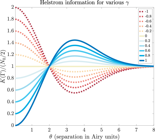
Eqs. (3.27) and (3.28) numerically. The results
are plotted in Fig. 1. Almost identical results
are recently reported in Ref. [17, Fig. 2(a)], which
uses the rare-photon model given by Eqs. (2.1) and a theory
consistent with the one here. The use of the intensity operator here
is arguably more direct and convenient, however, as
Eq. (4.7) comes naturally from optics and can be used
directly in Eqs. (3.27) and (3.28), without
returning to the rare-photon model or treating and
separately in the calculations.
Figure 1: Numerically computed Helstrom
information for the estimation of the separation
between two partially coherent sources. Each curve assumes
a fixed degree of coherence , as denoted by the legend.
As also noticed in Ref. [17], the Helstrom information
plotted in Fig. 1 appears to be identical to the
Fisher information with the Hermite-Gaussian measurements plotted in
Ref. [10, Fig. 1] for all values of ,
suggesting that the measurements are optimal for any and not
just for the case proven in Ref. [6].
5 Poisson channels
For the Poisson theory to remain useful for problems involving quantum
channels, the channels should preserve the Poissonianity of a state.
I call such channels Poisson channels. A trace-preserving completely
positive (TPCP) map on is Poisson if
(5.1)
where , is
1-dimensional, and , such that the output is
still a Poisson state in the Poisson limit. Let denote
the Poisson state with intensity operator in the sense of
Eqs. (2.1)–(2.3). The input-output relation in
the Poisson limit can be abbreviated as
(5.2)
where
is a map from an intensity operator to another intensity operator
induced by . Then the information quantities
, , ,
and in Eqs. (3.4), (3.10),
(3.11), and (3.27) also observe monotonicity
relations with respect to .
Proposition 10.
Let be a positive map defined in the sense of
Eqs. (5.1) and (5.2) with respect to a
TPCP map in the Poisson limit. Then
(5.3)
(5.4)
(5.5)
(5.6)
Proof.
These monotonicity relations follow from the monotonicity of the
information quantities with respect to the density operators in
Eqs. (3.4), (3.10), (3.11), and
(3.27).
∎
To construct examples of in the following, I assume
further that is local, in the sense of
(5.7)
where
is a TPCP map that gives
(5.8)
Under the local assumption, is affine, as shown by
Proposition 11 below, although Example 3
later demonstrates that need not be trace-preserving and
Example 4 demonstrates that need not be
linear.
Expressing and in the matrix forms
[22, Eq. (1.64)]
(5.10)
where denotes a zero operator and is an operator
that maps to , it can be shown that
(5.11)
For the requirement to be satisfied,
it is necessary for the map to satisfy
(5.12)
(5.13)
Multiplying both sides of Eq. (5.11) by and taking the
Poisson limit, the output intensity operator becomes
(5.14)
where is the Poisson limit of
,
which does not depend on . Equation (5.14) is
affine with respect to (though not necessarily linear).
∎
In the following examples, the Kraus form of each is most
conveniently expressed in terms of some orthonormal bases of
, , , and
, which are written as , ,
, and
, respectively. The state,
for example, can be expressed as
(5.15)
where is the density matrix of with respect to the basis
above.
Example 2(object-number-preserving channel).
Let a Kraus form of be
(5.16)
(5.17)
such that
(5.18)
where
(5.19)
is a TPCP map. In the Poisson limit,
(5.20)
The trace-preserving nature of means that the channel
preserves the object number. More specific examples include the
unitary map
(5.21)
which models a lossless linear device via a unitary operator , and
the map
(5.22)
which models a 100%-efficient object-counting measurement via the
POVM that gives Eqs. (2.7) and
(2.8). Propositions 6 and
9 are hence special cases of
Proposition 10.
As the object number need not be conserved, need not be
trace-preserving. The next examples of are noteworthy
departures from the usual TPCP maps in quantum information theory.
Example 3(loss).
Let and
(5.23)
(5.24)
where is the transmission coefficient for each mode.
Then
(5.25)
In the Poisson limit,
(5.26)
This is not trace-preserving if any ,
although it is still completely positive [22, Theorem 2.22].
Example 4(spontaneous emission).
Let and
(5.27)
(5.28)
(5.29)
where and
are properties of the channel and
is assumed to be the eigenbasis of without loss of
generality. Then
(5.30)
In the Poisson limit,
(5.31)
where . In particular, if the input
intensity operator is the zero operator ,
(5.32)
If , Eq. (5.32) implies that this
is not trace-preserving and not even linear, as a trace-preserving or
linear map on the zero operator must give the zero operator.
Setting , the spontaneous-emission probability per temporal
mode, to be ensures that the occurrence of objects
remains rare and remains finite under the Poisson
limit. In reality, however, a channel with a high
spontaneous-emission probability may make the final state non-Poisson
and may also involve other processes such as stimulated emission, so
one should double-check the accuracy of the Poisson approximation
before applying the Poisson theory to a real spontaneous-emission
channel.
Equation (5.31) is a quantum analog of the fact that the sum of
two independent Poisson processes is also a Poisson process. It may
be useful for modeling dark counts or background noise
[43, 44, 45]. Another version of this fact is the
following.
Example 5(composition).
The tensor product of two Poisson states may be expressed as
(5.33)
To derive this relation, consider
(5.34)
Ignore all terms in Eq. (5.34), including
the two-object component . The output intensity operator in the Poisson limit becomes
(5.35)
Since and are
1-dimensional, any tensor product of an operator with or
is isomorphic to the original operator, and
Eq. (5.35) can be abbreviated as .
Example 6(marginalization).
Let be an intensity operator on
and be a density operator
on
. Let
(5.36)
denote the partial trace with respect to
. A Kraus form is
(5.37)
Expressing in terms of the basis
, it is not
difficult to show that
(5.38)
where is the projection operator into given by
Eq. (5.29).
Equations (5.20), (5.26), (5.31), (5.33),
and (5.38) in the examples demonstrate that, for Poisson
channels, the maps can be much simplified if expressed in terms of the
intensity operators. Whether there exists a more comprehensive
mathematical treatment of Poisson channels in the spirit of quantum
channel theory is an interesting open problem.
6 Conclusion
In conclusion, I have shown that the Poisson limit leads to elegant
results in quantum information theory, with the intensity operator
emerging as the central quantity. The familiar appearances of the
formulas mean that one may borrow existing results from general
information theory and apply them to the intensity operators in the
study of Poisson states. Although the unnormalized nature of the
operators may require extra care, one can still take advantage of many
known results concerning unnormalized positive-semidefinite matrices
[35, 36, 38, 22], as the formulas here
coincide with many of them.
There are many potential generalizations and extensions. It should be
possible to define the Poisson limit more generally for a tensor
product of non-identical states and an infinite-dimensional ,
in analogy with the more general Poisson limit theorems
[1, 2]. The mathematical rigor of the limit may
be improved through quantum stochastic calculus [25]
or nonstandard analysis [26, 27]. The mathematical
theory of Poisson channels may be refined further.
In terms of applications, some specialized aspects of the Poisson
theory have already found success in the study of weak thermal light
for optical sensing and imaging [18, 8], but a
consolidation of the results under the umbrella of Poisson quantum
information may reveal new insights. Given the importance of the
classical Poisson theory in diverse areas [1, 2],
the quantum Poisson theory is envisioned to see wider applications in
quantum technologies beyond optics, wherever a sequence of rare
objects may be encountered.
Acknowledgments
I acknowledge helpful discussions with Zdeněk Hradil, Nick
Vamivakas, Vincent Tan, and Marco Tomamichel. This work is supported
by the National Research Foundation (NRF) Singapore, under its Quantum
Engineering Programme (Award QEP-P7).
Appendix A Poisson limit theorem
To state the Poisson limit theorem rigorously, I first rephrase the
measurement model in terms of measure theory. Consider a multi-output
object-counting measurement of the th temporal mode. Let
denote the set of outputs and denote its
-algebra. For example, for an ideal direct-imaging
measurement, each is a possible
position of the object on the image plane, while each
is a region of the image plane. Let
be the total object number detected by the
measurement. Assume
(A.1)
where denotes the expectation,
is the Iverson bracket defined as
(A.2)
and is the probability that the
statement is true. Conditioned on , let
be the output that detects the object. Assume
(A.3)
where is a POVM on
. The object count in a set of outputs can then be
modeled by the random measure
, defined as
(A.4)
and can be taken as independent random variables.
Integrated over temporal modes, the random measure becomes
(A.5)
where
(A.6)
is the detected object number in total and the set
is simply a relabeling of ,
which is a set of independent and identically distributed
(i.i.d.) random elements. As is Bernoulli, is binomial. In
the Poisson limit, becomes Poisson, denoted by , and
is called the Kac empirical point
process [24].
Theorem 1(see, for example, Ref. [24, Sec. 3.5.2]).
With a Poisson and a sequence of i.i.d. random elements
that are independent of , the Kac process
, defined as
(A.7)
is a Poisson process.
The intensity measure of
the Poisson process is given by
(A.8)
In the main text, the abbreviations
,
, , and
are used, where is a
disjoint partition of . are independent
Poisson random variables by a basic property of Poisson processes, so
their probability distribution is given by Eq. (2.7).
Appendix B Poisson states on Fock spaces
is called a toy Fock
space in Refs. [25, 46]. The Poisson limit of
on the toy Fock space should remain well defined if one is
willing to adopt nonstandard analysis, taking to be an unlimited
natural number and to be infinitesimal
[26, 27]. In the context of ordinary calculus, one may
think of as , where is an infinitesimal
interval in time or a similar continuous degree of freedom. In the
Poisson channel theory, Eq. (5.12) implies that each Kraus
operator should scale as
, which is why quantum stochastic
calculus may be needed to define the operators rigorously in the
Poisson limit.
A more standard way to deal with an infinite number of temporal modes
in quantum stochastic calculus is to abandon the toy Fock space and
use instead the Fock space ,
where is defined as [25]
(B.1)
and the space, modeling the temporal modes for one object,
is defined as
(B.2)
(B.3)
See Refs. [25, 46, 26] for discussions of
the relation between the toy Fock space and
. It is an open problem,
outside the scope of this paper, how Poisson states may be expressed
on .
If the objects are collected in one place and their arrival times are
ignored, one can assume a simpler Fock space
(B.4)
and transform into a state on given by
(B.5)
(B.6)
where denotes an appropriate map, is the binomial random
variable for the total object number, and
is assumed. This representation may be
useful because any function of density operators that satisfies a
monotonicity relation with respect to TPCP maps can be computed using
instead of , by virtue of the following
proposition.
Proposition 12.
is TPCP. Moreover, there exists another TPCP map such
that .
has the spirit of a Kac process and may serve as a
rigorous definition of a Poisson state without resorting to
nonstandard analysis. For example, a Poisson process can arise
directly from a measurement on as follows. Let be the
object number determined by a measurement in terms of the Kraus
operators , where is the projection operator
into . The conditional state becomes
. If each object is then measured by the POVM
, the outcomes are the i.i.d. random elements
. The Kac process
is therefore a Poisson
process by Theorem 1.
Many other results in this paper can also be rederived from
Eq. (B.8). Equations (2.1) are more intuitive from the
physics point of view, however, and are therefore used in the main
text.
To derive Eq. (3.6), take similar steps
to those in the proof of Proposition 1 to obtain
(C.1)
(C.2)
and then take the Poisson limit.
Note that Eq. (3.7) takes the infimum of the
Poisson limit, but to prove that it is the same as the Poisson limit
of the infimum, one may need to prove the uniform convergence of
to over , beyond
the pointwise convergence just proved. This complication suggests that
the Poisson limit is an intricate mathematical issue, and the
Fock-space representation given by Eq. (B.8), the Poisson limit
of which has already been taken, may be a better starting point for
rigorous proofs. In particular, Eq. (B.8) leads directly to
Eqs. (3.6) and (3.7) without
any ambiguity.
∎
To prove that is TPCP, I construct a physical procedure that
takes as input and produces as output.
1.
Designate the input system as system A and an auxiliary system
with Hilbert space
and initial state as system B.
2.
For each :
(a)
Measure the number of objects in the th temporal mode of
system A with the Kraus operators . Let
be the random variable from the measurement.
(b)
If , do nothing.
(c)
If , put the object detected in the th temporal mode
of system A (in conditional state
) into an empty temporal
mode of system B (any mode in state ).
3.
Discard all the empty temporal modes in system B so that its
Hilbert space becomes , where
is the number of detected objects.
4.
Give system B as the output.
With as the input state, is Bernoulli, is binomial,
the output state conditioned on is , and the
unconditional output state becomes Eq. (B.5).
To prove that a TPCP map giving exists, I
construct a physical procedure that takes as input and
gives as output.
1.
Assume a system A with Hilbert space
and initial state
. Assume a system B with Hilbert space
. For the map,
assume that system A is auxiliary and system B is the input.
2.
Measure the number of objects in system B with the Kraus
operators .
3.
Generate a random classical bit sequence
with bits equal to and
bits equal to . The probability of each sequence is assumed
to be
(C.8)
4.
For each :
(a)
If , do nothing.
(b)
If , put an object in system B into the th temporal
mode of system A.
5.
Give system A as the output.
With as the input state, is binomial, and the
unconditional probability of each bit sequence becomes
(C.9)
meaning that is Bernoulli. Conditioned on , the output state
is
(C.10)
The unconditional output state is hence
(C.11)
∎
Appendix D Computation of the Helstrom information
for Example 1
To compute Eqs. (3.27) and (3.28) numerically, I
follow the method in Refs. [47, 48]. Express each
operator in the problem as
(D.1)
where the set spans . The set need
not be orthogonal or normalized. Let
for a scalar parameter
. Then Eq. (3.28) can be expressed as
For Example 1, and are
defined in Eqs. (4.8). Define also
(D.4)
Then
(D.5)
With the Gaussian given by Eq. (4.10), can
also be computed analytically (with the help of the Symbolic Math
Toolbox on Matlab (ver. 2020b, Mathworks)):
(D.6)
For each from to with step size and each
from to with step size , Eq. (D.2)
is solved for using the lyap function on Matlab
and is computed using Eq. (D.3). The results are
plotted in Fig. 1.
To prevent the error “The solution of this Lyapunov equation
does not exist or is not unique” in using the lyap
function on Matlab, a tiny positive number is artificially
introduced to and . To check
that does not affect the results significantly, the numerical
analysis is repeated with various , and it is found that the
plots do not show any perceptible change with ranging from
to . Figure 1 uses
.
The Matlab code is reproduced below. The lbmap routine to
generate a color map for colorblind viewers can be downloaded from
Ref. [49].
function helstrom
theta = .05:.05:8;
gamma = -1:.2:1;
delta = 1e-13;
hold off;
for m = 1:length(gamma)
  Gamma = [1 gamma(m) 0 0; conj(gamma(m)) 1 0 0; 0 0 delta 0; 0 0 0 delta];
  dGamma = [0 0 1 gamma(m); 0 0 conj(gamma(m)) 1; ...
            1 gamma(m) 0 0; conj(gamma(m)) 1 0 0];
  for n = 1:length(theta)
    G11 = 1;
    G12 = exp(-theta(n)^2/8);
    G13 = 0;
    G14 = -theta(n)/8*exp(-theta(n)^2/8);
    G22 = 1;
    G23 = G14;
    G24 = 0;
    G33 = 1/16;
    G34 = (theta(n)^2-4)/64*exp(-theta(n)^2/8);
    G44 = 1/16;
    G = [G11 G12 G13 G14; conj(G12) G22 G23 G24; ...
         conj(G13) conj(G23) G33 G34; conj(G14) conj(G24) conj(G34) G44];
    S = lyap(Gamma*G,-2*dGamma);
    K(n) = 2*trace(G*S*G*dGamma);
  end
  if gamma(m) < 0
    plot(theta,K,’:’);
  else
    plot(theta,K);
  end
  hold on;
end
axis([min(theta) max(theta) 0 2]);
legend(num2str(gamma.’));
xlabel(’$\theta$ (separation in Airy units)’);
ylabel(’$K(\Gamma)/(N_0/2)$’) ;
title(’Helstrom information for various $\gamma$’);
newcolor = lbmap(length(gamma),’RedBlue’);
colororder(newcolor);
Weedbrook et al. [2012]C. Weedbrook, S. Pirandola, R. García-Patrón, N. J. Cerf, T. C. Ralph,
J. H. Shapiro, and S. Lloyd, Rev. Mod. Phys. 84, 621 (2012).
Tsang et al. [2016b]M. Tsang, R. Nair, and X.-M. Lu, in Proc. SPIE, Quantum and Nonlinear Optics IV, Vol. 10029 (SPIE, Bellingham,
WA, 2016) p. 1002903.
Hradil et al. [2019]Z. Hradil, J. Řeháček, L. Sánchez-Soto, and B.-G. Englert, Optica 6, 1437 (2019).
Liang et al. [2021]K. Liang, S. A. Wadood, and A. N. Vamivakas, Optica 8, 243
(2021).
Wadood et al. [2021]S. A. Wadood, K. Liang,
Y. Zhou, J. Yang, M. A. Alonso, X.-F. Qian, T. Malhotra, S. M. Hashemi Rafsanjani, A. N. Jordan, R. W. Boyd, and A. N. Vamivakas, Optics Express 29, 22034 (2021).
Leitz-Martini [2001]M. Leitz-Martini, Quantum Stochastic Calculus
using Infinitesimals, Ph.D. thesis, University of Tübingen, Tübingen, Germany
(2001).
Nelson [1987]E. Nelson, Radically Elementary
Probability Theory (Princeton University Press, Princeton, New Jersey, 1987).
Uhlmann and Crell [2009]A. Uhlmann and B. Crell, in Entanglement and Decoherence, edited by A. Buchleitner, C. Viviescas, and M. Tiersch (Springer, Berlin, 2009) pp. 1–60.
Audenaert et al. [2007]K. M. R. Audenaert, J. Calsamiglia, R. Muñoz-Tapia, E. Bagan, L. Masanes,
A. Acin, and F. Verstraete, Physical Review Letters 98, 160501 (2007).