FFT-based free space Poisson solvers: why Vico-Greengard-Ferrando should replace Hockney-Eastwood

Abstract

Many problems in beam physics and plasma physics require the solution of Poisson’s equation with free-space boundary conditions. The algorithm proposed by Hockney and Eastwood is a popular scheme to solve this problem numerically, used by many cutting-edge codes, because of its speed and its simplicity. However, the potential and its gradient obtained with this method have low accuracy, and the numerical error converges slowly with the number of grid points. We demonstrate that the closely related algorithm recently proposed by Vico, Greengard, and Ferrando is just as easy to implement, just as efficient computationally, and has much higher accuracy, with a rapidly converging error.

I Motivation

In many simulations in beam physics and plasma physics, one needs to solve Poisson’s equation for the electrostatic potential $\phi$ due to the charge density $\rho$

$$\Delta\phi=-\rho$$ (1)

with free-space boundary conditions, such that the electric field $\mathbf{E}=-\nabla\phi$ vanishes infinitely far from the charge distribution Daughton, Scudder, and Karimabadi (2006); Qiang et al. (2006); Yang et al. (2010); Cerfon et al. (2013); Cerfon (2016); Guadagni and Cerfon (2017). This is the case when the physical system is such that the charge distribution is indeed in free space. Following standard potential theory, the solution to this problem can also serve as the particular solution entering in the construction of the full solution of Poisson’s equation on general domains and with more general boundary conditions Askham and Cerfon (2017); Fryklund, Lehto, and Tornberg (2018).

The natural solution to Eq.(1) with free-space boundary conditions is to write

$$\phi(\mathbf{r})=\int_{\mathbb{R}^{d}}\rho(\mathbf{r}^{\prime})G(\mathbf{r}-\mathbf{r}^{\prime})d\mathbf{r}^{\prime}$$ (2)

where $G(\mathbf{r})=-\frac{1}{2\pi}\ln r$ for the two-dimensional problem, and $G(\mathbf{r})=\frac{1}{4\pi r}$ for the three-dimensional problem, and $r=|\mathbf{r}|$. In most applications of physical interest, the charge distribution $\rho$ has compact support within the computational domain. There are two well-known difficulties with the numerical computation of (2). First, because of the long range of the Green’s functions, fast algorithms are necessary for the efficient computation of the convolution. Second, because of the singularity of the Green’s functions at $\mathbf{r}=\mathbf{r}^{\prime}$, special quadrature schemes must be designed to obtain high accuracy. In the last two decades, numerical schemes have been developed to address both difficulties in an efficient manner, even for cases where the charge distribution $\rho$ is highly inhomogeneous and requires adaptive discretization Ethridge and Greengard (2001); McCorquodale et al. (2005); Langston, Greengard, and Zorin (2011); Malhotra and Biros (2015).

The purpose of this letter is not to revisit these well-established algorithms. Instead, our goal is to focus on the common situation in beam physics and plasma physics where (1) is solved in a Cartesian coordinate system, and where the grid points are uniformly spaced. In such cases, the Fast-Fourier transform (FFT) is an efficient tool to address the first difficulty. Pioneering in that direction, Hockney and Eastwood Hockney and Eastwood (1988) have shown that by appropriately zero padding the charge distribution $\rho$, the aperiodic convolution (2) could be computed “exactly", i.e. to within errors due to the discretization and the quadrature scheme, with FFTs. Specifially, according to the convolution theorem, the convolution (2) is transformed to a product of functions in the Fourier domain. Thus, discretizing the charge distribution on the uniform grid, zero padding this discretized distribution in each spatial direction on an interval of the same length as the original domain, and defining a periodic Green’s function $\tilde{G}$ on that extended domain, they compute the electrostatic potential according to:

$$\phi=h_{x}h_{y}h_{z}FFT^{-1}\{FFT\{\tilde{\rho}\}FFT\{\tilde{G}\}\}$$ (3)

where $h_{x}$, $h_{y}$, and $h_{z}$ represent the grid spacing in each Cartesian dimension, $\tilde{\rho}$ is the padded charge distribution on the extended domain, $FFT\{\cdot\}$ represents an FFT in all spatial dimensions, and $FFT^{-1}\{\cdot\}$ represents an inverse FFT in all spectral dimensions. The numerical solver based on this approach is remarkably simple to implement, and efficient, since the computational complexity scales like $\mathcal{O}((2N)^{d}(\log 2N)^{d})$, where $N$ is the number of grid points in each direction for the original computational domain, before padding. As a result, it is widely used, including in high-performance codes for accelerator science and for plasma physics applications Budiardja and Cardall (2011); Shishlo et al. (2015); Adelmann et al. (2019).

However, a weakness of this scheme is the slow decay of the numerical error with increasing grid size: if the mesh spacing is $h$ in each spatial direction, the scheme is a second order scheme, with the error decaying like $h^{2}$. This is because the method relies on the standard trapezoidal rule for the discretization of (2), together with a regularization of the Green’s function, chosen such that $G(\mathbf{0})=1$, which is not designed to achieve high accuracy Rasmussen (2011). Alternate simple regularizations have been suggestedChatelain and Koumoutsakos (2010); Budiardja and Cardall (2011), which do not improve the order of convergence of the method, as discussed in Rasmussen (2011); Hejlesen, Winckelmans, and Walther (2019).

In contrast, Vico, Greengard, and Ferrando have recently proposed a closely related scheme, which is as easy to implement, as efficient computationally, but has a high order of convergence, giving the potential and the electric field with high accuracy for a modest number of grid points Vico, Greengard, and Ferrando (2016). The purpose of this letter is to encourage beam and plasma physicists to switch from Hockney & Eastwood to this scheme, by briefly explaining the numerical method it is based on, showing that its implementation is indeed as simple, and providing test cases demonstrating the superiority of the method.

The remainder of this article is structured as follows. In Section II, we give a brief overview of the algorithm proposed by Vico, Greengard, and Ferrando. In Section III, we compare the accuracy of the algorithm of Hockney and Eastwood, and several of its common variants, with the accuracy of the algorithm by Vico et al.. We then conclude with a brief summary.

II Brief description of the scheme by Vico, Greengard, and Ferrando

Without loss of generality, let us assume that the computational domain is the unit box $D=[-0.5,0.5]^{d}$. As we discussed previously, we operate under the assumption that $\rho$ is compactly supported in $D$. For both $d=2$ and $d=3$, and for $L>0$, we define the following windowed Green’s functions:

$$G^{L}(\mathbf{r})=G(\mathbf{r})\mathbf{1}_{I}\left(\frac{r}{2L}\right)$$ (4)

where $\mathbf{1}_{I}$ is the indicator function for the interval $I=[-0.5,0.5]$, such that $\mathbf{1}_{I}(\mathbf{x})=1$ if $\mathbf{x}\in I$, and $\mathbf{1}_{I}(\mathbf{x})=0$ otherwise. Note that in the computational domain, the maximum distance between a source at $\mathbf{r}^{\prime}$ and a target at $\mathbf{r}$ is $\sqrt{d}$. The first key observation by Vico et al. is that by setting $L>\sqrt{d}$, we have for all $\mathbf{r}$ in $D$:

$$\phi(\mathbf{r})=\int_{D}\rho(\mathbf{r}^{\prime})G(\mathbf{r}-\mathbf{r}^{\prime})d\mathbf{r}^{\prime}=\int_{D}\rho(\mathbf{r}^{\prime})G^{L}(\mathbf{r}-\mathbf{r}^{\prime})d\mathbf{r}^{\prime}$$ (5)

If we define the Fourier transform $\mathcal{F}\{f\}$ of a function $f$, and the inverse Fourier transform $\mathcal{F}^{-1}\{\hat{f}\}$ of a function $\hat{f}$, the electrostatic potential in the computational domain $D$ can thus be computed according to:

$$\phi=\mathcal{F}^{-1}\{\mathcal{F}\{\rho\}\mathcal{F}\{G^{L}\}\}$$ (6)

The second key observation of Vico et al. is that $\mathcal{F}\{G^{L}\}$ can be computed analytically, and that it is regular at $\mathbf{k}=\mathbf{0}$, where $\mathbf{k}$ is the Fourier wavevector, unlike the original Green’s function, whose Fourier transform is $\mathcal{F}\{G\}=\frac{1}{|\mathbf{k}|^{2}}$. We have

$$\mathcal{F}\{G^{L}\}=\frac{1-J_{0}(L|\mathbf{k}|)}{|\mathbf{k}|^{2}}-\frac{L\ln LJ_{1}(L|\mathbf{k}|)}{|\mathbf{k}|}\qquad(\mbox{in 2D})$$ (7)

$$\mathcal{F}\{G^{L}\}=2\left(\frac{\sin\left(\frac{L|k|}{2}\right)}{|k|}\right)^{2}\qquad(\mbox{in 3D})$$ (8)

We can therefore write the following explicit formula for the solution to Poisson’s equation with free-space boundary conditions in two dimensions

$$\phi(\mathbf{r})=\frac{1}{4\pi^{2}}\iint_{\mathbb{R}^{2}}e^{i\mathbf{k}\cdot\mathbf{r}}\mathcal{F}\{\rho\}(\mathbf{k})\left[\frac{1-J_{0}(L|\mathbf{k}|)}{|\mathbf{k}|^{2}}-\frac{L\ln LJ_{1}(L|\mathbf{k}|)}{|\mathbf{k}|}\right]d\mathbf{k}$$ (9)

and an analogous formula for three dimensions. Remarkably, the term in the square brackets in the integrand is an analytic function, which is a direct consequence of the Paley-Wiener theorem. It is also a nonincreasing function of $\mathbf{k}$. Discretization of the integral by the trapezoidal rule will thus allow the computation of $\phi$ with high accuracy, with the order of convergence of the scheme determined by the rate of decay of $\mathcal{F}\{\rho\}(\mathbf{k})$, and spectral accuracy achieved for sufficiently smooth $\rho(\mathbf{r})$ Trefethen (2000); Trefethen and Weideman (2014), as commonly encountered in practical applications. The algorithm can therefore rely solely on standard FFTs for the fast evaluation of the aperiodic convolution, as for Hockney and Eastwood.

Because of the oscillatory nature of $\mathcal{F}\{G^{L}\}$, the charge distribution must in principle be extended by zero-padding to a grid of size $(4N)^{d}$, and the computations done on this extended grid, in order to compute the integral without aliasing error. This would seem to be a significant drawback as compared to the computations on a grid of size $(2N)^{d}$ in the Hockney and Eastwood algorithm. In practice, this is however not an issue, because Vico et al. show that for a given computational grid and a given Green’s function, all Poisson solves can be done on a grid of size $(2N)^{d}$ after an initial precomputation step on a grid of size $(4N)^{d}$. Specifically, one computes the inverse FFT of $\mathcal{F}\{G^{L}\}$ on a grid of size $(4N)^{d}$, and the result restricted to the appropriate grid of size $(2N)^{d}$ then serves as the numerical Green’s function for all the other computations, on a grid of size $(2N)^{d}$. This is crucial, since in most applications, Poisson’s equation must be solved for a new charge distribution at each time step, on a fixed grid. The precomputation step is then a negligible part of the total computational cost. To summarize, the only difference in terms of numerical implementation between the Hockney & Eastwood method and the method by Vico et al. is that with the former, the Green’s function is given analytically, whereas with the latter, it must be precomputed via an inverse FFT of (7) or (8) on a domain of size $(4N)^{d}$. MATLAB versions of our codes can be downloaded on https://www.math.nyu.edu/ cerfon/codes.html for readers further interested in the details of the (easy) implementation.

III Numerical comparison of the solvers

In this section, we compare the accuracy and convergence of the schemes by Hockney & Eastwood and by Vico et al.. For conciseness, we only show one two-dimensional example, and one three-dimensional example, which have radially symmetric and spherically symmetric charge distributions. We obtain similar results for distributions without such symmetry.

III.1 Two-dimensional example

We consider here the Gaussian charge density

$$\rho=\frac{1}{2\pi\sigma^{2}}\exp\bigg{(}-\frac{x^{2}+y^{2}}{2\sigma^{2}}\bigg{)}$$ (10)

with $\sigma=0.05$, and the computational domain is $[-0.5,0.5]^{2}$.

The analytic solution $\phi^{*}$ for the potential is given by:

$$\phi^{*}(x,y)=-\frac{1}{4\pi}\bigg{[}\text{Ei}\bigg{(}\frac{x^{2}+y^{2}}{2\sigma^{2}}\bigg{)}+\log(x^{2}+y^{2})\bigg{]}$$ (11)

where Ei is the exponential integral function. Let $h=1/N$ and $\phi_{i,j}$ be the numerical solution at grid point $[-0.5+ih,-0.5+hj]$. We compute the relative error $e_{i,j}$ as:

$$e_{i,j}=\bigg{|}\frac{\phi_{i,j}-\phi^{*}(-0.5+ih,-0.5+jh)}{\phi^{*}(-0.5+ih,-0.5+jh)}\bigg{|}$$ (12)

Figure 1 shows the maximal relative error of $\phi$ over all grid points for the method by Vico et al. (indicated by "mollified kernel"), the Hockney and Eastwood method (indicated by "singularity replaced by $1/2\pi$" and two variants of Hockney and Eastwood (indicated by "nearby value"Budiardja and Cardall (2011) and "cell average"Chatelain and Koumoutsakos (2010) respectively), for $N$ ranging from $10$ to $100$.

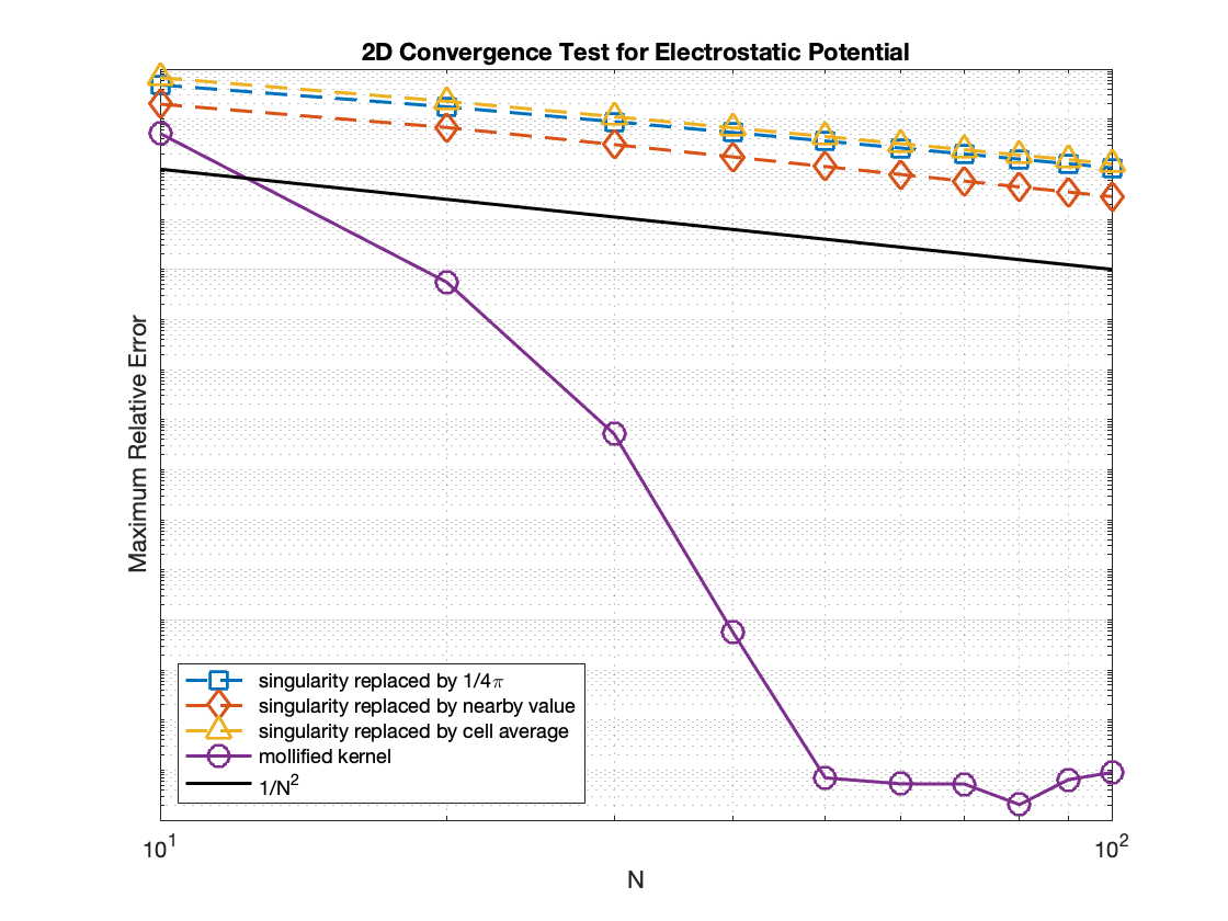
Figure 1: Numerical error for the electrostatic potential in our two-dimensional test, for the different algorithms discussed in this article.

To further illustrate our point, we also compute the electric field $\mathbf{E}$. For the FFT-based schemes we consider here, a natural approach is to compute $\mathbf{E}$ through Fourier differentiation (indicated by "Fourier"), i.e. multiplication by the wavevector in Fourier space before computing the inverse FFT. However, centered differences are still commonly used in combination with the Hockney & Eastwood algorithm, so we also implemented a finite difference approach (indicated by "Finite Diff") for an Hockney & Eastwood case. Note that since the analytic solution of the electric field is equal to zero at certain grid points, we used the absolute error $e_{abs}$ for this calculation:

$$e^{abs}_{i,j}=|E_{i,j}-E^{*}(-0.5+ih,-0.5+jh)|$$ (13)

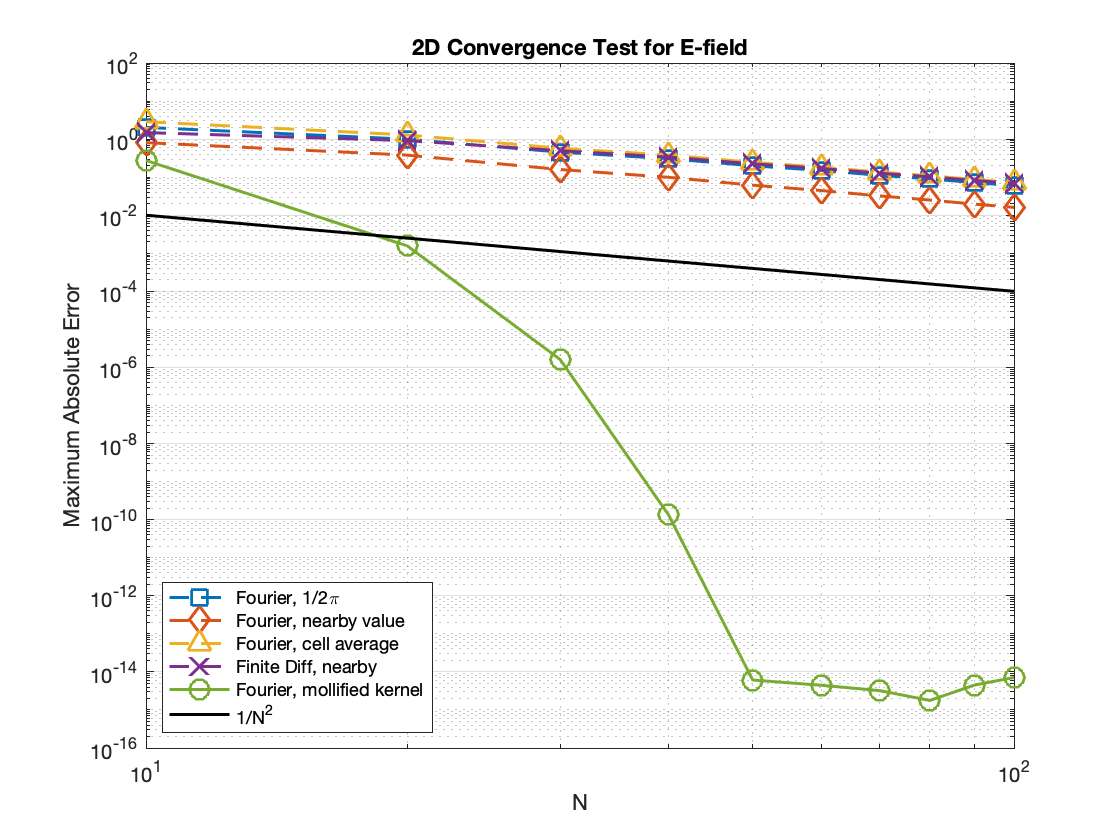
Figure 2: Numerical error for the x-component of the electric field in our two-dimensional test, for the different algorithms discussed in this article. By symmetry, the convergence properties for the y-component are identical.

Figure 2 shows the maximal absolute error for $E_{x}=\frac{\partial\phi}{\partial x}$, for $N$ ranging from $10$ to $100$. We omit the convergence plots for $E_{y}$ due to the symmetry of the charge density. Figures 1 and 2 demonstrate the spectral convergence of the scheme by Vico et al., the second order convergence of the Hockney & Eastwood algorithms, and that Vico et al. leads to much higher accuracy, even for a modest number of grid points.

III.2 Three-dimensional example

We repeat the numerical experiment for the 3-dimensional domain $[-0.5,0.5]^{3}$, for the following source function and exact solution:

$$\rho =\frac{1}{(2\pi)^{3/2}\sigma^{3}}\exp\bigg{(}-\frac{x^{2}+y^{2}+z^{2}}{2\sigma^{2}}\bigg{)}$$ (14)

$$\phi^{*}(x,y,z) =\frac{1}{4\pi\sqrt{x^{2}+y^{2}+z^{2}}}\text{erf}\bigg{(}\frac{\sqrt{x^{2}+y^{2}+z^{2}}}{\sqrt{2}\sigma}\bigg{)}$$ (15)

with $\sigma=0.05$. Figure 3 and 4 show results similar to the two-dimensional case, again for $N$ ranging from $10$ to $100$.

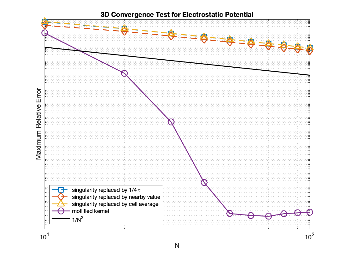
Figure 3: Numerical error for the electrostatic potential in our three-dimensional test, for the different algorithms discussed in this article.

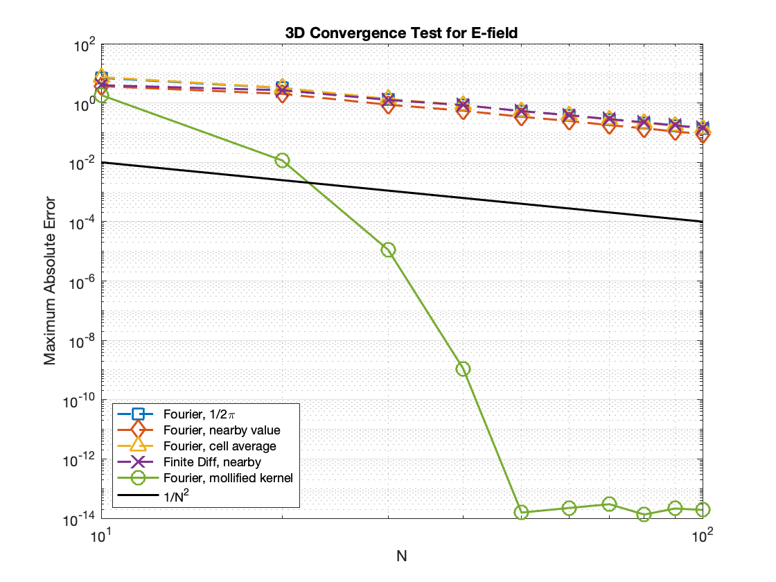
Figure 4: Numerical error for the x-component of the electric field in our three-dimensional test, for the different algorithms discussed in this article. By symmetry, the convergence properties for the y/z-components are identical.

IV Concluding remarks

For the smooth source distributions commonly encountered in beam and plasma physics, the FFT-based free space Poisson solver by Vico, Greengard, and Ferrando is superior to the method by Hockney and Eastwood, with much higher convergence rate and accuracy. Since both algorithms have a comparable computational complexity, and are as simple to implement, our results may encourage users of the popular Hockney & Eastwood method to switch to the scheme by Vico et al..

We note that Poisson’s equation with free-space boundary conditions is also a key element in many astrophysical simulations Bertschinger (1998); Colombi and Alard (2017), for the computation of the self-consistent gravitational force. Many solvers rely on the Hockney-Eastwood algorithm Tanaka et al. (2017) and other low-order accurate FFT accelerated algorithms Passy and Bryan (2014); Moon, Kim, and Ostriker (2019); Krasnopolsky et al. (2021); they would benefit from replacing these schemes with the Vico-Greengard-Ferrando scheme.

Finally, we stress that when the source distribution is not smooth and is highly inhomogeneous, neither of the two FFT-based algorithms described here gives solutions with high accuracy. When small errors are required for these cases, advanced adaptive algorithms should be favoredEthridge and Greengard (2001); McCorquodale et al. (2005); Langston, Greengard, and Zorin (2011); Malhotra and Biros (2015).

Data availability

The data that support the findings of this study are available from the corresponding author upon reasonable request.

References

- Daughton, Scudder, and Karimabadi (2006) W. Daughton, J. Scudder, and H. Karimabadi, “Fully kinetic simulations of undriven magnetic reconnection with open boundary conditions,” Physics of Plasmas 13, 072101 (2006).
- Qiang et al. (2006) J. Qiang, S. Lidia, R. D. Ryne, and C. Limborg-Deprey, “Three-dimensional quasistatic model for high brightness beam dynamics simulation,” Phys. Rev. ST Accel. Beams 9, 044204 (2006).
- Yang et al. (2010) J. Yang, A. Adelmann, M. Humbel, M. Seidel, T. Zhang, et al., “Beam dynamics in high intensity cyclotrons including neighboring bunch effects: Model, implementation, and application,” Physical Review Special Topics-Accelerators and Beams 13, 064201 (2010).
- Cerfon et al. (2013) A. J. Cerfon, J. P. Freidberg, F. I. Parra, and T. A. Antaya, “Analytic fluid theory of beam spiraling in high-intensity cyclotrons,” Phys. Rev. ST Accel. Beams 16, 024202 (2013).
- Cerfon (2016) A. J. Cerfon, “Vortex dynamics and shear-layer instability in high-intensity cyclotrons,” Phys. Rev. Lett. 116, 174801 (2016).
- Guadagni and Cerfon (2017) J. Guadagni and A. J. Cerfon, “Fast and spectrally accurate evaluation of gyroaverages in non-periodic gyrokinetic-Poisson simulations,” Journal of Plasma Physics 83 (2017).
- Askham and Cerfon (2017) T. Askham and A. J. Cerfon, “An adaptive fast multipole accelerated Poisson solver for complex geometries,” Journal of Computational Physics 344, 1–22 (2017).
- Fryklund, Lehto, and Tornberg (2018) F. Fryklund, E. Lehto, and A.-K. Tornberg, “Partition of unity extension of functions on complex domains,” Journal of Computational Physics 375, 57–79 (2018).
- Ethridge and Greengard (2001) F. Ethridge and L. Greengard, “A new fast-multipole accelerated Poisson solver in two dimensions,” SIAM Journal on Scientific Computing 23, 741–760 (2001), https://doi.org/10.1137/S1064827500369967 .
- McCorquodale et al. (2005) P. McCorquodale, P. Colella, G. T. Balls, and S. B. Baden, “A scalable parallel Poisson solver in three dimensions with infinite-domain boundary conditions,” in 2005 International Conference on Parallel Processing Workshops (ICPPW’05) (IEEE, 2005) pp. 163–172.
- Langston, Greengard, and Zorin (2011) H. Langston, L. Greengard, and D. Zorin, “A free-space adaptive FMM-based PDE solver in three dimensions,” Communications in Applied Mathematics and Computational Science 6, 79–122 (2011).
- Malhotra and Biros (2015) D. Malhotra and G. Biros, “PVFMM: A parallel kernel independent FMM for particle and volume potentials,” Communications in Computational Physics 18, 808–830 (2015).
- Hockney and Eastwood (1988) R. W. Hockney and J. W. Eastwood, Computer simulation using particles (crc Press, 1988).
- Budiardja and Cardall (2011) R. D. Budiardja and C. Y. Cardall, “Parallel FFT-based Poisson solver for isolated three-dimensional systems,” Computer Physics Communications 182, 2265–2275 (2011).
- Shishlo et al. (2015) A. Shishlo, S. Cousineau, J. Holmes, and T. Gorlov, “The particle accelerator simulation code PyORBIT,” Procedia computer science 51, 1272–1281 (2015).
- Adelmann et al. (2019) A. Adelmann, P. Calvo, M. Frey, A. Gsell, U. Locans, C. Metzger-Kraus, N. Neveu, C. Rogers, S. Russell, S. Sheehy, et al., “OPAL a versatile tool for charged particle accelerator simulations,” arXiv preprint arXiv:1905.06654 (2019).
- Rasmussen (2011) J. T. Rasmussen, “Particle methods in bluff body aerodynamics,” Technical University of Denmark (2011).
- Chatelain and Koumoutsakos (2010) P. Chatelain and P. Koumoutsakos, “A Fourier-based elliptic solver for vortical flows with periodic and unbounded directions,” Journal of Computational Physics 229, 2425–2431 (2010).
- Hejlesen, Winckelmans, and Walther (2019) M. M. Hejlesen, G. Winckelmans, and J. H. Walther, “Non-singular Green’s functions for the unbounded Poisson equation in one, two and three dimensions,” Applied Mathematics Letters 89, 28–34 (2019).
- Vico, Greengard, and Ferrando (2016) F. Vico, L. Greengard, and M. Ferrando, “Fast convolution with free-space Green’s functions,” Journal of Computational Physics 323, 191–203 (2016).
- Trefethen (2000) L. N. Trefethen, Spectral methods in MATLAB (SIAM, 2000).
- Trefethen and Weideman (2014) L. N. Trefethen and J. Weideman, “The exponentially convergent trapezoidal rule,” SIAM Review 56, 385–458 (2014).
- Bertschinger (1998) E. Bertschinger, “Simulations of structure formation in the universe,” Annual Review of Astronomy and Astrophysics 36, 599–654 (1998), https://doi.org/10.1146/annurev.astro.36.1.599 .
- Colombi and Alard (2017) S. Colombi and C. Alard, “A ‘metric’ semi-lagrangian Vlasov–Poisson solver,” Journal of Plasma Physics 83, 705830302 (2017).
- Tanaka et al. (2017) S. Tanaka, K. Yoshikawa, T. Minoshima, and N. Yoshida, “Multidimensional Vlasov–Poisson simulations with high-order monotonicity-and positivity-preserving schemes,” The Astrophysical Journal 849, 76 (2017).
- Passy and Bryan (2014) J.-C. Passy and G. L. Bryan, “An adaptive particle-mesh gravity solver for ENZO,” The Astrophysical Journal Supplement Series 215, 8 (2014).
- Moon, Kim, and Ostriker (2019) S. Moon, W.-T. Kim, and E. C. Ostriker, “A fast Poisson solver of second-order accuracy for isolated systems in three-dimensional cartesian and cylindrical coordinates,” The Astrophysical Journal Supplement Series 241, 24 (2019).
- Krasnopolsky et al. (2021) R. Krasnopolsky, M. P. Martínez, H. Shang, Y.-H. Tseng, and C.-C. Yen, “Efficient direct method for self-gravity in 3d, accelerated by a fast Fourier transform,” The Astrophysical Journal Supplement Series 252, 14 (2021).