PACEMAKER
Avoiding HeART attacks in storage clusters with disk-adaptive redundancy

Abstract

Data redundancy provides resilience in large-scale storage clusters, but imposes significant cost overhead. Substantial space-savings can be realized by tuning redundancy schemes to observed disk failure rates. However, prior design proposals for such tuning are unusable in real-world clusters, because the IO load of transitions between schemes overwhelms the storage infrastructure (termed transition overload).

This paper analyzes traces for millions of disks from production systems at Google, NetApp, and Backblaze to expose and understand transition overload as a roadblock to disk-adaptive redundancy: transition IO under existing approaches can consume 100% cluster IO continuously for several weeks. Building on the insights drawn, we present pacemaker, a low-overhead disk-adaptive redundancy orchestrator. pacemaker mitigates transition overload by (1) proactively organizing data layouts to make future transitions efficient, and (2) initiating transitions proactively in a manner that avoids urgency while not compromising on space-savings. Evaluation of pacemaker with traces from four large (110K–450K disks) production clusters show that the transition IO requirement decreases to never needing more than 5% cluster IO bandwidth (0.2–0.4% on average). pacemaker achieves this while providing overall space-savings of 14–20% and never leaving data under-protected. We also describe and experiment with an integration of pacemaker into HDFS.

1 Introduction

Distributed storage systems use data redundancy to protect data in the face of disk failures[13, 15, 55]. While it provides resilience, redundancy imposes significant cost overhead. Most large-scale systems today erasure code most of the data stored, instead of replicating, which helps to reduce the space overhead well below 100% [63, 68, 24, 13, 43, 47]. Despite this, space overhead remains a key concern in large-scale systems since it directly translates to an increase in the number of disks and the associated increase in capital, operating and energy costs [24, 13, 43, 47].

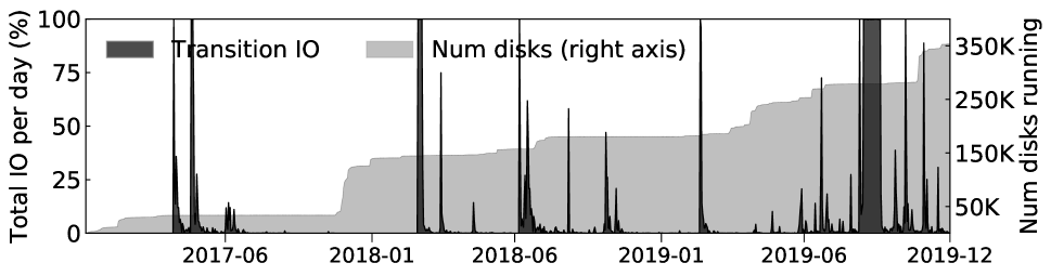
(a) Transition IO for HeART [26] on Google Cluster1.

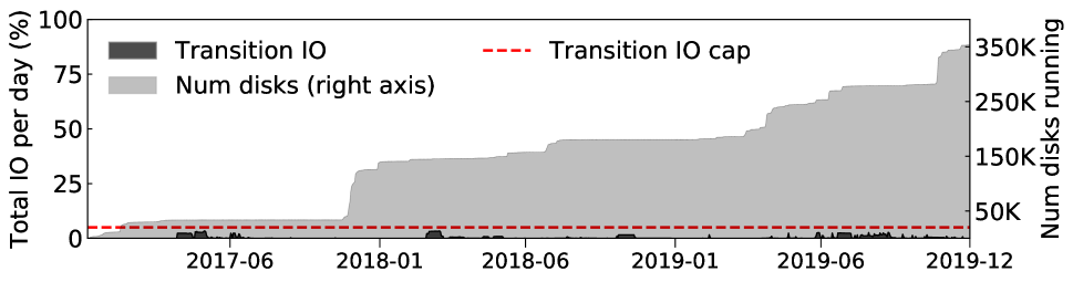
(b) Transition IO for pacemaker on Google Cluster1.

Figure 1: Fraction of total cluster IO bandwidth needed to use disk-adaptive redundancy for a Google storage cluster’s first three years. The state-of-the-art proposal [26] shown in 1(a) would require up to 100% of the cluster bandwidth for extended periods, whereas pacemaker shown in 1(b) always fits its IO under a cap (5%). The light gray region shows the disk count (right Y-axis) over time.

Storage clusters are made up of disks from a mix of makes/models acquired over time, and different makes/models have highly varying failure rates[31, 40, 26]. Despite that, storage clusters employ a “one-size-fits-all-disks” approach to choosing redundancy levels, without considering failure rate differences among disks. Hence, space overhead is often inflated by overly conservative redundancy levels, chosen to ensure sufficient protection for the most failure-prone disks in the cluster. Although tempting, the overhead cannot be removed by using very “wide” codes (which can provide high reliability with low storage overhead) for all data, due to the prohibitive reconstruction cost induced by the most failure-prone disks (more details in § 2). An exciting alternative is to dynamically adapt redundancy choices to observed failure rates (AFRs) for different disks, which recent proposals suggest could substantially reduce the space overhead [26].

Adapting redundancy involves dynamic transitioning of redundancy schemes, because AFRs must be learned from observation of deployed disks and because AFRs change over time due to disk aging. Changing already encoded data from one redundancy scheme to another, for example from an erasure code with parameters $k_{1}$-of-$n_{1}$ to $k_{2}$-of-$n_{2}$ (where $k$-of-$n$ denotes $k$ data chunks and $n-k$ parity chunks; more details in § 2), can be exorbitantly IO intensive. Existing designs for disk-adaptive redundancy are rendered unusable by overwhelming bursts of urgent transition IO when applied to real-world storage clusters. Indeed, as illustrated in Fig. 1(a), our analyses of production traces show extended periods of needing 100% of the cluster’s IO bandwidth for transitions. We refer to this as the transition overload problem. At its core, transition overload occurs whenever an observed AFR increase for a subset of disks requires too much urgent transition IO in order to keep data safe. Existing designs for disk-adaptive redundancy perform redundancy transitions as a reaction to AFR changes. Since prior designs are reactive, for an increase in AFR, the data is already under-protected by the time the transition to increase redundancy is issued. And it will continue to be under-protected until that transition completes. For example, around 2019-09 in Fig. 1(a), data was under-protected for over a month, even though the entire cluster’s IO bandwidth was used solely for redundancy transitions. Simple rate-limiting to reduce urgent bursts of IO would only exacerbate this problem causing data-reliability goals to be violated for even longer.

To understand the causes of transition overload and inform solutions, we analyse multi-year deployment and failure logs for over 5.3 million disks from Google, NetApp and Backblaze. Two common transition overload patterns are observed. First, sometimes disks are added in tens or hundreds over time, which we call trickle deployments. A statistically confident AFR observation requires thousands of disks. Thus, by the time it is known that AFR for a specific make/model and age is too high for the redundancy used, the oldest thousands of that make/model will be past that age. At that point, all of those disks need immediate transition. Second, sometimes disks are added in batches of many thousands, which we call step deployments. Steps have sufficient disks for statistically confident AFR estimation. However, when a step reaches an age where the AFR is too high for the redundancy used, all disks of the step need immediate transition.

This paper introduces pacemaker, a new disk-adaptive redundancy orchestration system that exploits insights from the aforementioned analyses to eliminate the transition overload problem. pacemaker proactively organizes data layouts to enable efficient transitions for each deployment pattern, reducing total transition IO by over 90%. Indeed, by virtue of its reduced total transition IO, pacemaker can afford to use extra transitions to reap increased space-savings. pacemaker also proactively initiates anticipated transitions sufficiently in advance that the resulting transition IO can be rate-limited without placing data at risk. Fig. 1(b) provides a peek into the final result: pacemaker achieves disk-adaptive redundancy with substantially less total transition IO and never exceeds a specified transition IO cap (5% in the graph).

We evaluate pacemaker using logs containing all disk deployment, failure, and decommissioning events from four production storage clusters: three 160K–450K-disk Google clusters and a $\approx$110K-disk cluster used for the Backblaze Internet backup service [4]. On all four clusters, pacemaker provides disk-adaptive redundancy while using less than 0.4% of cluster IO bandwidth for transitions on average, and never exceeding the specified rate limit (e.g., 5%) on IO bandwidth. Yet, despite its proactive approach, pacemaker loses less than 3% of the space-savings as compared to to an idealized system with perfectly-timed and instant transitions. Specifically, pacemaker provides 14–20% average space-savings compared to a one-size-fits-all-disks approach, without ever failing to meet the target data reliability and with no transition overload. We note that this is substantial savings for large-scale systems, where even a single-digit space-savings is worth the engineering effort. For example, in aggregate, the four clusters would need $\approx$200K fewer disks.

We also implement pacemaker in HDFS, demonstrating that pacemaker’s mechanisms fit into an existing cluster storage system with minimal changes. Complementing our longitudinal evaluation using traces from large scale clusters, we report measurements of redundancy transitions in pacemaker-enhanced HDFS via small-scale cluster experiments. Prototype of HDFS with Pacemaker is open-sourced and is available at https://github.com/thesys-lab/pacemaker-hdfs.git.

This paper makes five primary contributions. First, it demonstrates that transition overload is a roadblock that precludes use of previous disk-adaptive redundancy proposals. Second, it presents insights into the sources of transition overload from longitudinal analyses of deployment and failure logs for 5.3 million disks from three large organizations. Third, it describes pacemaker’s novel techniques, designed based on insights drawn from these analyses, for safe disk-adaptive redundancy without transition overload. Fourth, it evaluates pacemaker’s policies for four large real-world storage clusters, demonstrating their effectiveness for a range of deployment and disk failure patterns. Fifth, it describes integration of and experiments with pacemaker’s techniques in HDFS, demonstrating their feasibility, functionality, and ease of integration into a cluster storage implementation.

2 Whither disk-adaptive redundancy

Cluster storage systems and data reliability. Modern storage clusters scale to huge capacities by combining up to hundreds of thousands of storage devices into a single storage system [15, 55, 64]. In general, there is a metadata service that tracks data locations (and other metadata) and a large number of storage servers that each have up to tens of disks. Data is partitioned into chunks that are spread among the storage servers/devices. Although hot/warm data is now often stored on Flash SSDs, cost considerations lead to the majority of data continuing to be stored on mechanical disks (HDDs) for the foreseeable future [6, 7, 53]. For the rest of the paper, any reference to a “device” or “disk” implies HDDs.

Disk failures are common and storage clusters use data redundancy to protect against irrecoverable data loss in the face of disk failures  [15, 24, 40, 4, 42, 43, 47]. For hot data, often replication is used for performance benefits. But, for most bulk and colder data, cost considerations have led to the use of erasure coding schemes. Under a $k$-of-$n$ coding scheme, each set of $k$ data chunks are coupled with $n$-$k$ “parity chunks” to form a “stripe”. A $k$-of-$n$ scheme provides tolerance to $(n-k)$ failures with a space overhead of $\frac{n}{k}$. Thus, erasure coding achieves substantially lower space overhead for tolerating a given number of failures. Schemes like 6-of-9 and 10-of-14 are commonly used in real-world deployments [13, 42, 43, 47]. Under erasure coding, additional work is involved in recovering from a device failure. To reconstruct a lost chunk, $k$ remaining chunks from the stripe must be read.

The redundancy scheme selection problem. The reliability of data stored redundantly is often quantified as mean-time-to-data-loss (MTTDL) [17], which essentially captures the average time until more than the tolerated number of chunks are lost. MTTDL is calculated using the disks’ AFR and its mean-time-to-repair (MTTR).

Large clusters are built over time, and hence usually consist of a mix of disks belonging to multiple makes/models depending on which options were most cost effective at each time. AFR values vary significantly between makes/models and disks of different ages [26, 31, 40, 49]. Since disks have different AFRs, computing MTTDL of a candidate redundancy scheme for a large-scale storage cluster is often difficult.

The MTTDL equations can still be used to guide decisions, as long as a sufficiently high AFR value is used. For example, if the highest AFR value possible for any deployed make/model at any age is used, the computed MTTDL will be a lower bound. So long as the lower bound on MTTDL meets the target MTTDL, the data is adequately reliable. Unfortunately, the range of possible AFR values in a large storage cluster is generally quite large (over an order of magnitude) [26, 31, 40, 51]. Since the overall average is closer to the lower end of the AFR range, the highest AFR value is a conservative over-estimate for most disks. The resulting MTTDLs are thus loose lower bounds, prompting decision-makers to use a one-size-fits-all scheme with excessive redundancy leading to wasted space.

Using wide schemes with large number of parities (e.g., 30-of-36) can achieve the desired MTTDL while keeping the storage overhead low enough to make disk-adaptive redundancy appear not worth the effort. But, while this might seem like a panacea, wide schemes in high-AFR regimes cause significant increase in failure reconstruction IO traffic. The failure reconstruction IO is derived by multiplying the AFR with the number of data chunks in each stripe. Thus, if either of these quantities are excessively high, or both are moderately high, it can lead to overwhelmingly high failure reconstruction IO. In addition, wide schemes also result in higher tail latencies for individual disk reconstructions because of having to read from many more disks. Combined, these reasons prevent use of wide schemes for all data all the time from being a viable solution for most systems.

Disk-adaptive redundancy. Since the problem arises from using a single AFR value, a promising alternative is to adapt redundancy for subsets of disks with similar AFRs. A recent proposal, heterogeneity-aware redundancy tuner (HeART) [26], suggests treating subsets of deployed disks with different AFR characteristics differently. Specifically, HeART adapts redundancy of each disk by observing its failure rate on the fly depending on its make/model and its current age. It is well known that AFR of disks follow a “bathtub” shape with three distinct phases of life: AFR is high in “infancy” (1-3 months), low and stable during its “useful life” (3-5 years), and high during the “wearout” (a few months before decommissioning). HeART uses a default (one-size-fits-all) redundancy scheme for each new disk’s infancy. It then dynamically changes the redundancy to a scheme adapted to the observed useful life AFR for that disk’s make/model, and then dynamically changes back to the default scheme at the end of useful life. The per-make/model useful life redundancy schemes typically have much lower space overhead than the default scheme. This suggests the ability to maintain target MTTDL with many fewer disks (i.e., lower cost).

Although exciting, the design of HeART overlooks a crucial element: the IO cost associated with changing the redundancy schemes. Changing already encoded data under one erasure code to another can be exorbitantly IO intensive. Indeed, our evaluation of HeART on real-world storage cluster logs reveal extended periods where data safety is at risk and where 100% cluster IO bandwidth is consumed for scheme changes. We call this problem transition overload.

An enticing solution that might appear to mitigate transition overload is to adapt redundancy schemes only by removing parities in low-AFR regimes and adding parities in high-AFR regimes. While this solution eliminates transition IO when reducing the level of redundancy, it does only marginally better when redundancy needs to be increased, because new parity creation cannot avoid reading all data chunks from each stripe. What makes this worse is that transitions that increase redundancy are time-critical, since delaying them would miss the MTTDL target and leave the data under-protected. Moreover, addition / removal of a parity chunk massively changes the stripe’s MTTDL compared to addition / removal of a data chunk. For example, a 6-of-9 MTTDL is 10000$\times$ higher than 6-of-8 MTTDL, but is only 1.5$\times$ higher than 7-of-10 MTTDL. AFR changes would almost never be large enough to safely remove a parity, given default schemes like 6-of-9, eliminating almost all potential benefits of disk-adaptive redundancy.

This paper analyzes disk deployment and failure data from large-scale production clusters to discover sources of transition overload and informs the design of a solution. It then describes and evaluates pacemaker, which realizes the dream of safe disk-adaptive redundancy without transition overload.

3 Longitudinal production trace analyses

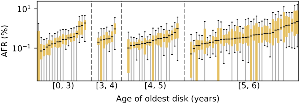
(a) Spread of make/model AFRs.

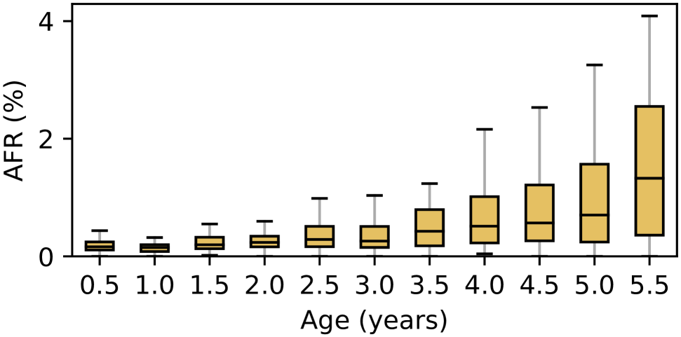
(b) AFR distribution over disk life.

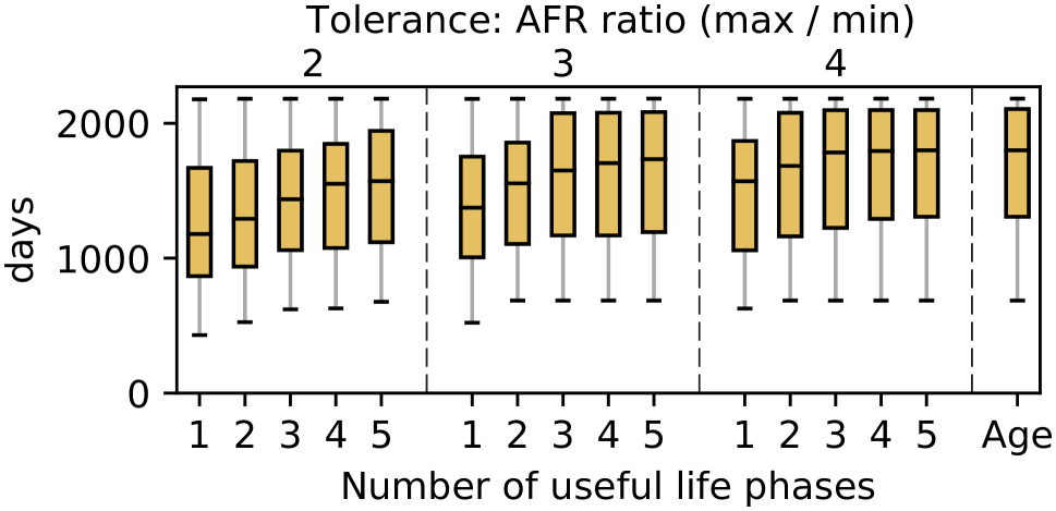
(c) Approximate useful-life length.

Figure 2: 2(a) AFR spread for over 50 makes/models from NetApp binned by the age of the oldest disk. Each box corresponds to a unique make/model, and at least 10000 disks of each make/model were observed (outlier AFR values omitted). 2(b) Distribution of AFR calculated over consecutive non-overlapping six-month periods for NetApp disks, showing the gradual rise of AFR with age (outliers omitted). 2(c) Approximation of useful life length for NetApp disks for 1-5 consecutive phases of useful life and three different tolerance levels. .

This section presents an analysis of multi-year disk reliability logs and deployment characteristics of 5.3 million HDDs, covering over 60 makes/models from real-world environments. Key insights presented here shed light on the sources of transition overload and challenges / opportunities for a robust disk-adaptive redundancy solution.

The data. Our largest dataset comes from NetApp and contains information about disks deployed in filers (file servers). Each filer reports the health of each disk periodically (typically once a fortnight) using their AutoSupport [28] system. We analyzed the data for a subset of their deployed disks, which included over 50 makes/models and over 4.3 million disks total. As observed in previous studies [26, 40, 49], we observe well over an order of magnitude difference between the highest and lowest useful-life AFRs (see Fig. 2(a)).

Our other datasets come from large storage clusters deployed at Google and the Backblaze Internet backup service. Although the basic disk characteristics (e.g., AFR heterogeneity and its behavior discussed below) are similar to the NetApp dataset, these datasets also capture the evolution and behavior in our target context (large-scale storage clusters), and thus are also used in the evaluation detailed in (§7). The particular Google clusters were selected based on their longitudinal data availability, but were not otherwise screened for favorability.

For each cluster, the multi-year log records (daily) all disk deployment, failure, and decommissioning events from birth of the cluster until the date of the log snapshot. Google Cluster1’s disk population over three years included $\approx$350K disks of 7 makes/models. Google Cluster2’s population over 2.5 years included $\approx$450K disks of 4 makes/models. Google Cluster3’s population over 3 years included $\approx$160K disks of 3 makes/models. The Backblaze cluster’s population since 2013 included $\approx$110K disks of 7 makes/models.

3.1 Causes of transition overload

Disk deployment patterns. We observe disk deployments occurring in two distinct patterns, which we label trickle and step. Trickle-deployed disks are added to a cluster frequently (weekly or even daily) over time by the tens and hundreds. For example, the slow rise in disk count seen between 2018-01 and 2018-07 in Fig. 1 represents a series of trickle-deployments. In contrast, a step-deployment introduces many thousands of disks into the cluster “at once” (over a span of a few days), followed by potentially months of no new step-deployments. The sharp rises in disk count around 2017-12 and 2019-11 in Fig. 1 represent step-deployments.

A given cluster may be entirely trickle-deployed (like the Backblaze cluster), entirely step-deployed (like Google Cluster2), or a mix of the two (like Google Cluster1 and Cluster3). Disks of a step are typically of the same make/model.

Learning AFR curves online. Disk-adaptive redundancy involves learning the AFR curve for each make/model by observing failures among deployed disks of that make/model. Because AFR is a statistical measure, the larger the population of disks observed at a given age, the lower is the uncertainty in the calculated AFR at that age. We have found that a few thousand disks need to be observed to obtain sufficiently accurate AFR measurements.

Transition overload for trickle-deployed disks. Since trickle-deployed disks are deployed in tiny batches over time, several months can pass before the required number of disks of a new make/model are past any given age. Thus, by the time the required number of disks can be observed at the age that is eventually identified as having too-high an AFR and requiring increased redundancy, data on the older disks will have been left under-protected for months. And, the thousands of already-older disks need to be immediately transitioned to a stronger redundancy scheme, together with the newest disks to reach that age. This results in transition overload.

Transition overload for step-deployed disks. Assuming that they are of the same make/model, a batch of step-deployed disks will have the same age and AFR, and indeed represent a large enough population for confident learning of the AFR curve as they age. But, this means that all of those disks will reach AFR values together, as they age. So, when their AFR rises to the point where the redundancy must be increased to keep data safe, all of the disks must transition together to the new safer redundancy scheme. Worse, if they are the first disks of the given make/model deployed in the cluster, which is often true in the clusters studied, then the system adapting the redundancy will learn of the need only when the age in question is reached. At that point, all data stored on the entire batch of disks is unsafe and needs immediate transitioning. This results in transition overload.

3.2 Informing a solution

Analyzing the disk logs has exposed a number of observations that provide hope and guide the design of pacemaker. The AFR curves we observed deviate substantially from the canonical representation where infancy and wearout periods are identically looking and have high AFR values, and AFR in useful life is flat and low throughout.

AFRs rise gradually over time with no clear wearout. AFR curves generally exhibit neither a flat useful life phase nor a sudden transition to so-called wearout. Rather, in general, it was observed that AFR curves rise gradually as a function of disk age. Fig. 2(b) shows the gradual rise in AFR over six month periods of disk lifetimes. Each box represents the AFR of disks whose age corresponds to the six-month period denoted along the X-axis. AFR curves for individual makes/models (e.g., Figs. 5(b) and 5(d)) are consistent with this aggregate illustration. Importantly, none of the over 60 makes/models from Google, Backblaze and NetApp displayed sudden onset of wearout.

Gradual increases in AFR, rather than sudden onset of wearout, suggests that one could anticipate a step-deployed batch of disks approaching an AFR threshold. This is one foundation on which pacemaker’s proactive transitioning approach rests.

Useful life could have multiple phases. Given the gradual rise of AFRs, useful life can be decomposed into multiple, piece-wise constant phases. Fig. 2(c) shows an approximation of the length of useful life when multiple phases are considered. Each box in the figure represents the distribution over different make/models of the approximate length of useful life. Useful life is approximated by considering the longest period of time which can be decomposed into multiple consecutive phases (number of phases indicated by the bottom X-axis) such that the ratio between the maximum and minimum AFR in each phase is under a given tolerance level (indicated by the top X-axis). The last box indicates the distribution over make/models of the age of the oldest disk, which is an upper bound to the length of useful life. As shown by Fig. 2(c), the length of useful life can be significantly extended (for all tolerance levels) by considering more than one phase. Furthermore, the data show that a small number of phases suffice in practice, as the approximate length of useful life changes by little when considering four or more phases.

Infancy often short-lived. Disks may go through (potentially) multiple rounds of so-called “burn-in” testing. The first tests may happen at the manufacturer’s site. There may be additional burn-in tests done at the deployment site allowing most of the infant mortality to be captured before the disk is deployed in production. For the NetApp and Google disks, we see the AFR drop sharply and plateau by 20 days for most of the makes/models. In contrast, the Backblaze disks display a slightly longer and higher AFR during infancy, which can be directly attributed to their less aggressive on-site burn-in.

pacemaker’s design is heavily influenced from these learnings, as will be explained in the next section.

4 Design goals

pacemaker is an IO efficient redundancy orchestrator for storage clusters that support disk-adaptive redundancy. Before going into the design goals for pacemaker, we first chronicle a disk’s lifecycle, introducing the terminology that will be used in the rest of the paper (defined in Table 1).

Disk lifecycle under pacemaker. Throughout its life, each disk under pacemaker simultaneously belongs to a Dgroup and an Rgroup. There are as many Dgroups in a cluster as there are unique disk makes/models. Rgroups on the other hand are a function of redundancy schemes and placement restrictions. Each Rgroup has an associated redundancy scheme, and its data (encoded stripes) must reside completely within that Rgroup’s disks. Multiple Rgroups can use the same redundancy scheme, but no stripe may span across Rgroups. The Dgroup of a disk never changes, but a disk may transition through multiple Rgroups during its lifetime. At the time of deployment (or “birth”), the disk belongs to Rgroup0, and is termed as an unspecialized disk. Disks in Rgroup0 use the default redundancy scheme, i.e. the conservative one-scheme-fits-all scheme used in storage clusters that do not have disk-adaptive redundancy. The redundancy scheme employed for a disk (and hence its Rgroup) changes via transitions. The first transition any disk undergoes is an RDn transition. A RDn transition changes the disk’s Rgroup to one with lower redundancy, i.e. more optimized for space. Whenever the disk departs from Rgroup0, it is termed as a specialized disk. Disks depart from Rgroup0 at the end of their infancy. Since infancy is short-lived (§3.2), pacemaker only considers one RDn transition for each disk.

Term	Definition
Dgroup	Group of disks of the same make/model.
Transition	The act of changing the redundancy scheme.
RDn transition	Transition to a lower level of redundancy.
RUp transition	Transition to a higher level of redundancy.
peak-IO-cap	IO bandwidth cap for transitions.
Rgroup	Group of disks using the same redundancy
	with placement restricted to the group of disks.
Rgroup0	Rgroup using the default one-scheme-fits-all
	redundancy used in storage clusters today.
Unspecialized disks	Disks that are a part of Rgroup0.
Specialized disks	Disks that are not part of Rgroup0.
Canary disks	First few thousand disks of a trickle-deployed
	Dgroup used to learn AFR curve.
Tolerated-AFR	Max AFR for which redundancy scheme meets
	reliability constraint.
Threshold-AFR	The AFR threshold crossing which triggers
	an RUp transition for step-deployed disks.

Table 1: Definitions of pacemaker’s terms.

The first RDn transition occurs at the start of the disk’s useful life, and marks the start of its specialization period. As explained in §3.2, a disk may experience multiple useful life phases. pacemaker performs a transition at the start of each useful life phase. After the first (and only) RDn transition, each subsequent transition is an RUp transition. An RUp transition changes the disk’s Rgroup to one with higher redundancy, i.e. less optimized for space, but the disk is still considered a specialized disk unless the Rgroup that the disk is being RUp transitioned to is Rgroup0. The space-savings (and thus cost-savings) associated with disk-adaptive redundancy are proportional to the fraction of life the disks remain specialized for.

Key decisions. To adapt redundancy throughout a disk’s lifecycle as chronicled above, three key decisions related to transitions must be made

1. When should the disks transition?

2. Which Rgroup should the disks transition to?

3. How should the disks transition?

Constraints. The above decisions need to be taken such that a set of constraints are met. An obvious constraint, central to any storage system, is that of data reliability. The reliability constraint mandates that all data must always meet a predefined target MTTDL. Another important constraint is the failure reconstruction IO constraint. This constraint bounds the IO spent on data reconstruction of failed disks, which as explained in §2 is proportional to AFR and scheme width. This is why wide schemes cannot be used for all disks all the time, but they can be used for low-AFR regimes of disk lifetimes (as discussed in §2).

Existing approaches to disk-adaptive redundancy make their decisions on the basis of only these constraints [26], but fail to consider the equally important IO caused by redundancy transitions. Ignoring this causes the transition overload problem, which proves to be a show-stopper for disk-adaptive redundancy systems. pacemaker treats transition IO as a first class citizen by taking it into account for each of its three key decisions. As such, pacemaker enforces carefully designed constraints on transition IO as well.

Designing IO constraints on transitions. Apart from serving foreground IO requests, a storage cluster performs numerous background tasks like scrubbing and load balancing [5, 48, 37]. Redundancy management is also a background task. In current storage clusters, redundancy management tasks predominantly consist of performing data redundancy (e.g. replicating or encoding data) and reconstructing data of failed or otherwise unavailable disks. Disk-adaptive redundancy systems add redundancy transitions to the list of IO-intensive background tasks.

There are two goals for background tasks: Goal 1: they are not too much work, and Goal 2: they interfere as little as possible with foreground IO. pacemaker applies two IO constraints on background transition tasks to achieve these goals: (1) average-IO constraint and (2) peak-IO constraint. The average-IO constraint achieves Goal 1 by allowing storage administrators to specify a cap on the fraction of the IO bandwidth of a disk that can be used for transitions over its lifetime. For example, if a disk can transition in 1 day using 100% of its IO bandwidth, then an average-IO constraint of 1% would mean that the disk will transition at most once every 100 days. The peak-IO constraint achieves Goal 2 by allowing storage administrators to specify the peak rate (defined as the peak-IO-cap) at which transitions can occur so as to limit their interference with foreground traffic. Continuing the previous example, if the peak-IO-cap is set at 5%, the disk that would have taken 1 day to transition at 100% IO bandwidth would now take at least 20 days. The average-IO constraint and the peak-IO-cap can be configured based on how busy the cluster is. For example, a cluster designed for data archival would have a lower foreground traffic, compared to a cluster designed for serving ads or recommendations. Thus, low-traffic clusters can set a higher peak-IO-cap resulting in faster transitions and potentially increased space-savings.

Design goals. The key design goals are to answer the three questions related to transitions such that the space-savings are maximized and the following constraints are met: (1) reliability constraint on all data all the time, (2) failure reconstruction IO constraint on all disks all the time, (3) peak-IO constraint on all disks all the time, and (4) average-IO constraint on all disks over time.

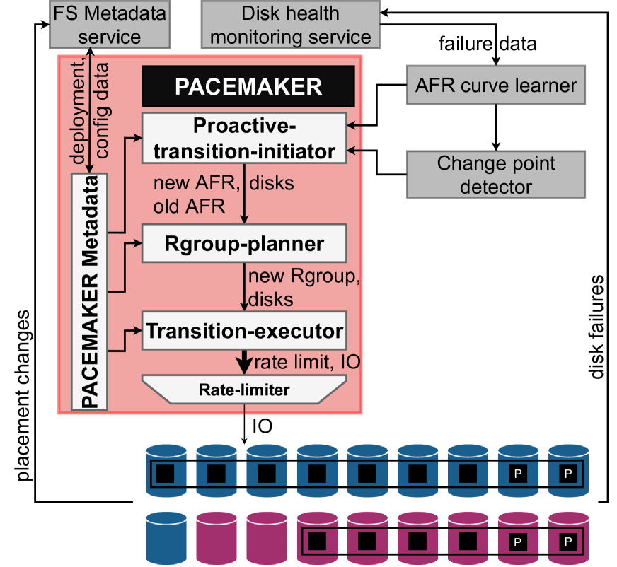
Figure 3: pacemaker architecture.

5 Design of pacemaker

Fig. 3 shows the high level architecture of pacemaker and how it interacts with some other components of a storage cluster. The three main components of pacemaker correspond to the three key decisions that the system makes as discussed in §4. The first main component of pacemaker is the proactive-transition-initiator (§5.1), which determines when to transition disks using the AFR curves and the disk deployment information. The information of the transitioning disks and their observed AFR is passed to the Rgroup-planner (§5.2), which chooses the Rgroup to which the disks should transition. The Rgroup-planner passes the information of the transitioning disks and the target Rgroup to the transition-executor (§5.3). The transition-executor addresses how to transition the disks to the planned Rgroup in the most IO-efficient way.

Additionally, pacemaker also maintains its own metadata and a simple rate-limiter. pacemaker metadata interacts with all of pacemaker’s components and also the storage cluster’s metadata service. It maintains various configuration settings of a pacemaker installation along with the disk deployment information that guides transition decisions. The rate-limiter rate-limits the IO load generated by any transition as per administrator specified limits. Other cluster components external-to-pacemaker that inform it are the AFR curve learner and the change point detector. As is evident from their names, these components learn the AFR curve of each Dgroup and identify change points for redundancy transitions. The AFR curve learner receives failure data from the disk health monitoring service, which monitors the disk fleet and maintains their vitals.

5.1 Proactive-transition-initiator

Proactive-transition-initiator’s role is to determine when to transition the disks. Below we explain pacemaker’s methodology for making this decision for the two types of transitions (RDn and RUp) and the two types of deployments (step and trickle).

5.1.1 Deciding when to RDn a disk

Recall that a disk’s first transition is an RDn transition. As soon as proactive-transition-initiator observes (in a statistically accurate manner) that the AFR has decreased sufficiently, and is stable, it performs an RDn transition from the default scheme (i.e., from Rgroup0) employed in infancy to a more space-efficient scheme. This is the only RDn transition in a disk’s lifetime.

5.1.2 Deciding when to RUp a disk

RUp transitions are performed either when there are too few disks in any Rgroup such that data placement is heavily restricted (which we term purging an Rgroup), or when there is a rise in AFR such that the reliability constraint is (going to be) violated. Purging an Rgroup involves RUp transitioning all of its disks to an Rgroup with higher redundancy. This transition isn’t an imminent threat to reliability, and therefore can be done in a relaxed manner without violating the reliability constraint as explained in §5.3.

However, most RUp transitions in a storage cluster are done in response to a rise in AFR. These are challenging with respect to meeting IO constraints due to the associated risk of violating the reliability constraints whenever the AFR rises beyond the AFR tolerated by the redundancy scheme (termed tolerated-AFR).

In order to be able to safely rate-limit the IO load due to RUp transitions, pacemaker takes a proactive approach. The key is in determining when to initiate a proactive RUp transition such that the transition can be completed before the AFR crosses the tolerated-AFR, while adhering to the IO and the reliability constraints without compromising much on space-savings. To do so, the proactive-transition-initiator assumes that its transitions will proceed as per the peak-IO constraint, which is ensured by the transition-executor. pacemaker’s methodology for determining when to initiate a proactive RUp transition is tailored differently for trickle versus for step deployments, since they raise different challenges.

Trickle deployments. For trickle-deployed disks, pacemaker considers two category of disks: (1) first disks to be deployed from any particular trickle-deployed Dgroup, and (2) disks from that Dgroup that are deployed later.

pacemaker labels the first $C$ deployed disks of a Dgroup as canary disks, where $C$ is a configurable, high enough number of disks to yield statistically significant AFR observations. For example, based on our disk analyses, we observe that $C$ in low thousands (e.g., 3000) is sufficient. The canary disks of any Dgroup are the first to undergo the various phases of life for that Dgroup, and these observations are used to learn the AFR curve for that Dgroup. The AFR value for the Dgroup at any particular age is not known (with statistical confidence) until all canary disks go past that age. Furthermore, due to the trickle nature of the deployment, the canary disks would themselves have been deployed over weeks if not months. Thus, AFR for the canary disks can be ascertained only in retrospect. pacemaker never changes the redundancy of the canary disks to avoid them from ever violating the reliability constraint. This does not significantly reduce space-savings, since $C$ is expected to be small relative to the total number of disks of a Dgroup (usually in the tens of thousands).

The disks that are deployed later in any particular Dgroup are easier to handle, since the Dgroup’s AFR curve would have been learned by observing the canaries. Thus, the date at which a disk among the later-deployed disks needs to RUp to meet the reliability constraints is known in advance by the proactive-transition-initiator, which it uses to issue proactive RUp transitions.

Step deployments. Recall that in a step deployment, most disks of a Dgroup may be deployed within a few days. So, canaries are not a good solution, as they would provide little-to-no advance warning about how the AFR curve’s rises would affect most disks.

pacemaker’s approach to handling step-deployments is based on two properties: (1) Step-deployments have a large number of disks deployed together, leading to a statistically accurate AFR estimation; (2) AFR curves based on a large set of disks tend to exhibit gradual, rather than sudden, AFR increases as the disk ages (§3.2). pacemaker leverages these two properties to employ a simple early warning methodology to predict a forthcoming need to RUp transition a step well in advance. Specifically, pacemaker sets a threshold, termed threshold-AFR, which is a (configurable) fraction of the tolerated-AFR of the current redundancy scheme employed. For step-deployments, when the observed AFR crosses the threshold-AFR, the proactive-transition-initiator initiates a proactive RUp transition.

5.2 Rgroup-planner

The Rgroup-planner’s role is to determine which Rgroup should disks transition to. This involves making two interdependent choices: (1) the redundancy scheme to transition into, (2) whether or not to create a new Rgroup.

Choice of the redundancy scheme. At a high level, the Rgroup-planner first uses a set of selection criteria to arrive at a set of viable schemes. It further narrows down the choices by filtering out the schemes that are not worth transitioning to when the transition IO and IO constraints are accounted for.

Selection criteria for viable schemes. Each viable redundancy scheme has to satisfy the following criteria in addition to the reliability constraint: each scheme (1) must satisfy the minimum number of simultaneous failures per stripe (i.e., $n-k$); (2) must not exceed the maximum allowed stripe dimension ($k$); (3) must have its expected failure reconstruction IO (AFR $\times$ $k$ $\times$ disk-capacity) be no higher than was assumed possible for Rgroup0 (since disks in Rgroup0 are expected to have the highest AFR); (4) must have a recovery time in case of failure (MTTR) that does not exceed the maximum MTTR (set by the administrator when selecting the default redundancy scheme for Rgroup0).

Determining if a scheme is worth transitioning to. Whether the IO cost of transitioning to a scheme is worth it or not and what space-savings can be achieved by that transition is a function of the number of days disks will remain in that scheme (also known as disk-days). This, in turn, depends on (1) when the disks enter the new scheme, and (2) how soon disks will require another transition out of that scheme.

The time it takes for the disks to enter the new scheme is determined by the transition IO and the rate-limit. When the disks will transition out of the target Rgroup is dependent on the future and can only be estimated. For this estimation, the Rgroup-planner needs to estimate the number of days the AFR curve will remain below the threshold that forces a transition out. This needs different strategies for the two deployment patterns (trickle and step).

Recall that pacemaker knows the AFR curve for trickle-deployed disks (from the canaries) in advance. Recall that step-deployed disks have the property that the AFR curve learned from them is statistically robust and tends to exhibit gradual, as opposed to sudden AFR increases. The Rgroup-planner leverages these properties to estimate the future AFR behavior based on the recent past. Specifically, it takes the slope of the AFR curve in the recent past and uses that to project the AFR curve rise in the future.

The number of disk-days in a scheme for it to be worth transitioning to is dictated by the IO constraints. For example, let us consider a disk running under pacemaker that requires a transition, and pacemaker is configured with an average-IO constraint of 1% and a peak-IO-cap of 5%. Suppose the disk requires 1 day to complete its transition at 100% IO bandwidth. With the current settings, pacemaker will only consider an Rgroup worthy of transitioning to (assuming it is allowed to use all 5% of its IO bandwidth) if at least 80 disk-days are spent after the disk entirely transitions to it (since transitioning to it would take up to 20 days at the allowed 5% IO bandwidth).

From among the viable schemes that are worth transitioning to based on the IO constraints, the Rgroup-planner chooses the one that provides the highest space-savings.

Decision on Rgroup creation. Rgroups cannot be created arbitrarily. This is because every Rgroup adds placement restrictions, since all chunks of a stripe have to be stored on disks belonging to the same Rgroup. Therefore, Rgroup-planner creates a new Rgroup only when (1) the resulting placement pool created by the new Rgroup is large enough to overcome traditional placement restrictions such as “no two chunks on the same rack”, and (2) the space-savings achievable by the chosen redundancy scheme is sufficiently greater than using an existing (less-space-efficient) Rgroup.

The disk deployment pattern also affects Rgroup formation. While the rules for whether to form an Rgroup remain the same for trickle and step-deployed disks, mixing disks deployed differently impacts the transitioning techniques that can be used for eventually transitioning disks out of that Rgroup. This in turn affects how the IO constraints are enforced. Specifically, for trickle deployments, creating an Rgroup for each set of transitioning disks would lead to too many small-sized Rgroups. So, for trickle-deployments, the Rgroup-planner creates a new Rgroup for a redundancy scheme if and only if one does not exist already. Creating Rgroups this way will also ensure that enough disks (thousands) will go into it to satisfy placement restrictions. Mixing disks from different trickle-deployments in the same Rgroup does not impact the IO constraints, because pacemaker optimizes the transition mechanism for few disks transitioning at a time, as is explained in §5.3. For step-deployments, due to the large fraction of disks that undergo transition together, having disks from multiple steps, or mixing trickle-deployed disks within the same Rgroup, creates adverse interactions (discussed in §5.3). Hence, the Rgroup-planner creates a new Rgroup for each step-deployment, even if there already exists one or more Rgroups that employ the chosen scheme. Each such Rgroup will contain many thousands of disks to overcome traditional placement restrictions. Per-step Rgroups also extend to the Rgroup with default redundancy schemes, implying a per-step Rgroup0. Despite having clusters with disk populations as high as 450K disks, pacemaker’s restrained Rgroup creation led to no cluster ever having more than 10 Rgroups.

Rules for purging an Rgroup. An Rgroup may be purged for having too few disks. This can happen when too many of its constituent disks transition to other Rgroups, or they fail, or they are decommissioned leading to difficulty in fulfilling placement restrictions. If the Rgroup to be purged is made up of trickle-deployed disks, the Rgroup-planner will choose to RUp transition disks to an existing Rgroup with higher redundancy while meeting the IO constraints. For step-deployments, purging implies RUp transitioning disks into the more-failure-tolerant RGroup (RGroup0) that may include trickle-deployed disks.

5.3 Transition-executor

The transition-executor’s role is to determine how to transition the disks. This involves choosing (1) the most IO-efficient technique to execute that transition, and (2) how to rate-limit the transition at hand. Once the transition technique is chosen, the transition-executor executes the transition via the rate-limiter as shown in Fig. 3.

Selecting the transition technique. Suppose the data needs to be conventionally re-encoded from a $k_{cur}$-of-$n_{cur}$ scheme to a $k_{new}$-of-$n_{new}$ scheme. The IO cost of conventional re-encoding involves reading–re-encoding–writing all the stripes whose chunks reside on each transitioning disk. This amounts to a read IO of ${k_{cur}}\times$disk-capacity (assuming almost-full disks), and a write IO of ${k_{cur}}\times$disk-capacity$\times\frac{n_{new}}{k_{new}}$ for a total IO $>2\times{k_{cur}}\times$disk-capacity for each disk.

In addition to conventional re-encoding, pacemaker supports two new approaches to changing the redundancy scheme for disks and selects the most efficient option for any given transition. The best option depends on the fraction of the Rgroup being transitioned at once.

Type 1 (Transition by emptying disks). If a small percentage of an Rgroup’s disks are being transitioned, it is more efficient to retain the contents of the transitioning disks in that Rgroup rather than re-encoding. Under this technique, the data stored on transitioning disks are simply moved (copied) to other disks within the current Rgroup. This involves reading and writing (elsewhere) the contents of the transitioning disks. Thus, the IO of transitioning via Type 1 is at most 2$\times$disk-capacity, independent of scheme parameters, and therefore at least ${k_{cur}}\times$ cheaper than conventional re-encoding.

Type 1 can be employed whenever there is sufficient free space available to move the contents of the transitioning disks into other disks in the current Rgroup. Once the transitioning disks are empty, they can be removed from the current Rgroup and added to the new Rgroup as “new” (empty) disks.

Type 2 (Bulk transition by recalculating parities). If a large fraction of disks in an Rgroup need to transition together, it is more efficient to transition the entire Rgroup rather than only the disks that need a transition at that time. Most cluster storage systems use systematic codes [14, 8, 13, 35], wherein transitioning an entire Rgroup involves only calculating and storing new parities and deleting the old parities. Specifically, the data chunks have to be only read for computing the new parities, but they do not have to be re-written. In contrast, if only a part of the disks are transitioned, some fraction of the data chunks also need to be re-written. Thus, the IO cost for transitioning via Type 2 involves a read IO of $\frac{k_{cur}}{n_{cur}}\times$disk-capacity, and a write IO of only the new parities, which amounts to a total IO of $\frac{n_{new}-k_{new}}{k_{new}}\times\frac{k_{cur}}{n_{cur}}\times$disk-capacity for each disk in the Rgroup. This is at most $2\times\frac{k_{cur}}{n_{cur}}\times$disk-capacity, which makes it at least $n_{cur}\times$ cheaper than conventional re-encoding.

Selecting the most efficient approach for a transition. For any given transition, the transition-executor selects the most IO-efficient of all the viable approaches. Almost always, trickle-deployed disks use Type 1 because they transition a-few-at-a-time, and step-deployed disks use Type 2 because Rgroup-planner maintains each step in a separate Rgroup.

Choosing how to rate limit a transition. Irrespective of the transitioning techniques, the transition-executor has to resolve the competing concerns of maximizing space-savings and minimizing risk of data loss via fast transitions, and minimizing foreground work interference by slowing down transitions so as to not overwhelm the foreground IO. Arbitrarily slowing down a transition to minimize interference is only possible when the transition is not in response to a rise in AFR. This is because a rising AFR hints at the data being under-protected if not transitioned to a higher redundancy soon. In pacemaker, a transition without an AFR rise occurs either when disks are being RDn transitioned at the end of infancy, or when they are being RUp transitioned because the Rgroup they belong to is being purged. For all the other RUp transitions, pacemaker carefully chooses how to rate limit the transition.

Determining how much bandwidth to allow for a given transition could be difficult, given that other transitions may be in-progress already or may be initiated at any time (we do observe concurrent transitions in our evaluations). So, to ensure that the aggregate IO of all ongoing transitions conforms to the peak-IO-cap cluster-wide, pacemaker limits each transition to the peak-IO-cap within its Rgroup. For trickle-deployed disks, which share Rgroups, the rate of transition initiations is consistently a small percentage of the shared Rgroup, allowing disk emptying to proceed at well below the peak-IO-cap. For step-deployed disks, this is easy for pacemaker, since a step only makes one transition at a time and its IO is fully contained in its separate Rgroup. The transition-executor’s approach to managing peak-IO on a per-Rgroup basis is also why the proactive-transition-initiator can safely assume a rate-limit of the peak-IO-cap without consulting the transition-executor. If there is a sudden AFR increase that puts data at risk, pacemaker is designed to ignore its IO constraints to continue meeting the reliability constraint—this safety valve was never needed for any cluster evaluated.

After finalizing the transitioning technique, the transition-executor performs the necessary IO for transitioning disks (read, writes, parity recalculation, etc.). We find that the components required for the transition-executor are already present and adequately modular in existing distributed storage systems. In §6, we show how we implement pacemaker in HDFS with minimal effort.

Note that this design is for the common case where storage clusters are designed for a single dedicated storage service. Multiple distinct distributed storage services independently using the same underlying devices would need to coordinate their use of bandwidth (for their non-transition related load as well) in some way, which is outside the scope of this paper.

6 Implementation of pacemaker in HDFS

We have implemented a prototype of pacemaker for the Hadoop distributed file system (HDFS) [55]. HDFS is a popular open source distributed file system, widely employed in the industry for storing large volumes of data. We use HDFS v3.2.0, which natively supports erasure coding. Prototype of HDFS with Pacemaker is open-sourced and is available at https://github.com/thesys-lab/pacemaker-hdfs.git.

Background on HDFS architecture. HDFS has a central metadata server called Namenode (NN, akin to the master node) and a collection of servers containing the data stored in the file system, called Datanodes (DN, akin to worker nodes). Clients interact with the NN only to perform operations on file metadata (containing a collection of the DNs that store the file data). Clients directly request the data from the DNs. Each DN stores data on its local drives using a local file system.

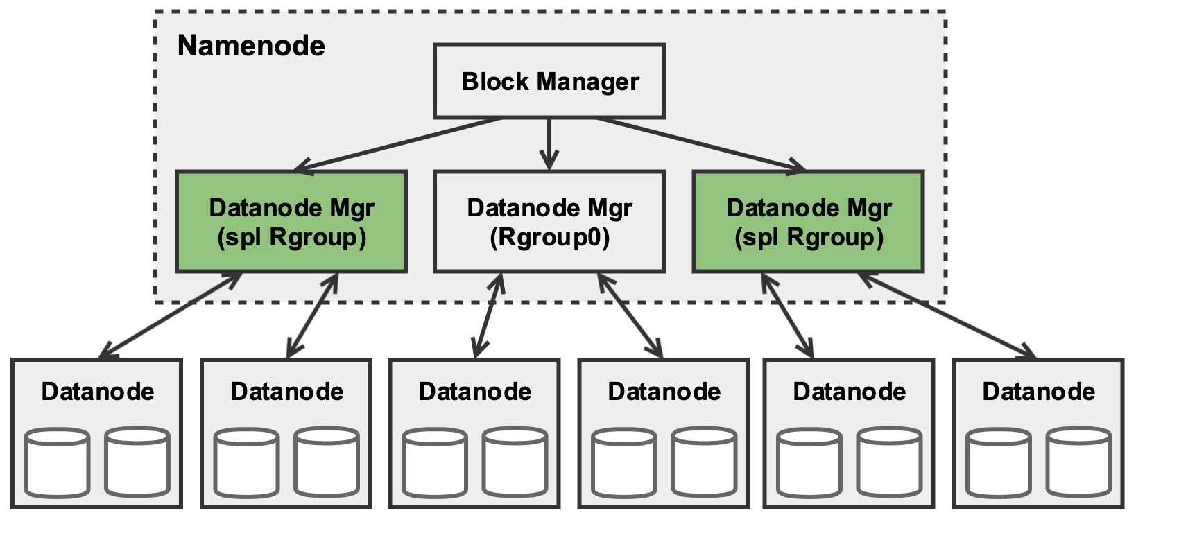
Figure 4: pacemaker-enhanced HDFS architecture.

Realizing Rgroups in HDFS. This design makes a simplifying assumption that all disks belonging to a DN are of the same Dgroup and are deployed together (this could be relaxed easily). Under this simplifying assumption, conceptually, an Rgroup would consist of a set of DNs that need to be managed independent of other such sets of DNs as shown in Fig 4.

The NN maintains a DatanodeManager (DNMgr), which is a gateway for the NN to interact with the DNs. The DNMgr maintains a list of the DNs, along with their usage statistics. The DNMgr also contains a HeartBeatManager (HrtBtMgr) which handles the periodic keepalive heartbeats from DNs. A natural mechanism to realize Rgroups in HDFS is to have one DNMgr per Rgroup. Note that the sets of DNs belonging to the different DNMgrs are mutually exclusive. Implementing Rgroups with multiple DNMgrs has several advantages.

Right level of control and view of the system. Since the DNMgr resides below the block layer, when the data needs to be moved for redundancy adaptations, the logical view of the file remains unaffected. Only the mapping from HDFS blocks to DNs gets updated in the inode. The statistics maintained by the DNMgr can be used to balance load across Rgroups.

Minimizing changes to the HDFS architecture and maximizing re-purposing of existing HDFS mechanisms. This design obviates the need to change HDFS’s block placement policy, since it is implemented at the DNMgr level. Block placement policies are notoriously hard to get right. Moreover, block placement decisions are affected by fault domains and network topologies, both of which are orthogonal to pacemaker’s goals, and thus best left untouched. Likewise, the code for reconstruction of data from a failed DN need not be touched, since all of the reads (to reconstruct each lost chunk) and writes (to store it somewhere else) will occur within the set of nodes managed by its DNMgr. Existing mechanisms for adding / decommissioning nodes managed by the DNMgr can be re-purposed to implement pacemaker’s Type 1 transitions (described below).

Cost of maintaining multiple DNMgrs is small. Each DNMgr maintains two threads: a HrtBtMgr and a DNAdminMgr. The former tracks and handles heartbeats from each DN, and the latter monitors the DNs for performing decommissioning and maintenance. The number of DNMgr threads in the NN will increase from two to 2$\times$ the number of Rgroups. Fortunately, even for large clusters, we observe that the number of Rgroups would not exceed the low tens (§7.4). The NN is usually a high-end server compared to the DNs, and an additional tens of threads shouldn’t affect performance.

Rgroup transitions in HDFS. An important part of pacemaker functionality is transitioning DNs between Rgroups. Recall from §5.3 that one of pacemaker’s preferred way of transitioning disks across Rgroups is by emptying the disks. In HDFS, the planned removal of a DN from a HDFS cluster is called decommissioning. pacemaker re-uses decommissioning to remove a DN from the set of DNs managed by one DNMgr and then adds it to the set managed by another, effectively transitioning a DN from one Rgroup to another.

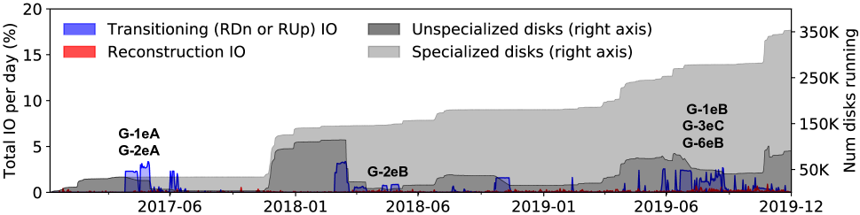
(a) Redundancy management IO due to pacemaker over its 2.5$+$ year lifetime broken down by IO type. This identical to Fig. 1(b) with the left Y axis only going to 20% to show the detailed IO activity happening in the cluster.

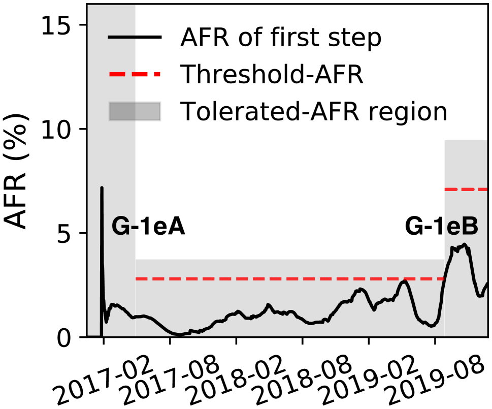
(b) G-1 (step) AFR curve

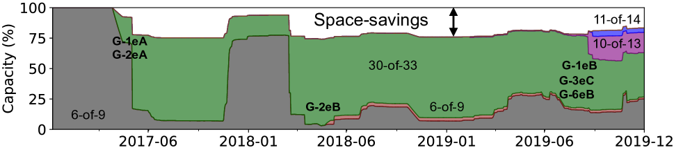
(c) Space-savings due to pacemaker. Each colored region represents the fraction of cluster capacity that is using a particular redundancy scheme. 6-of-9 is the default redundancy scheme (Rgroup0’s).

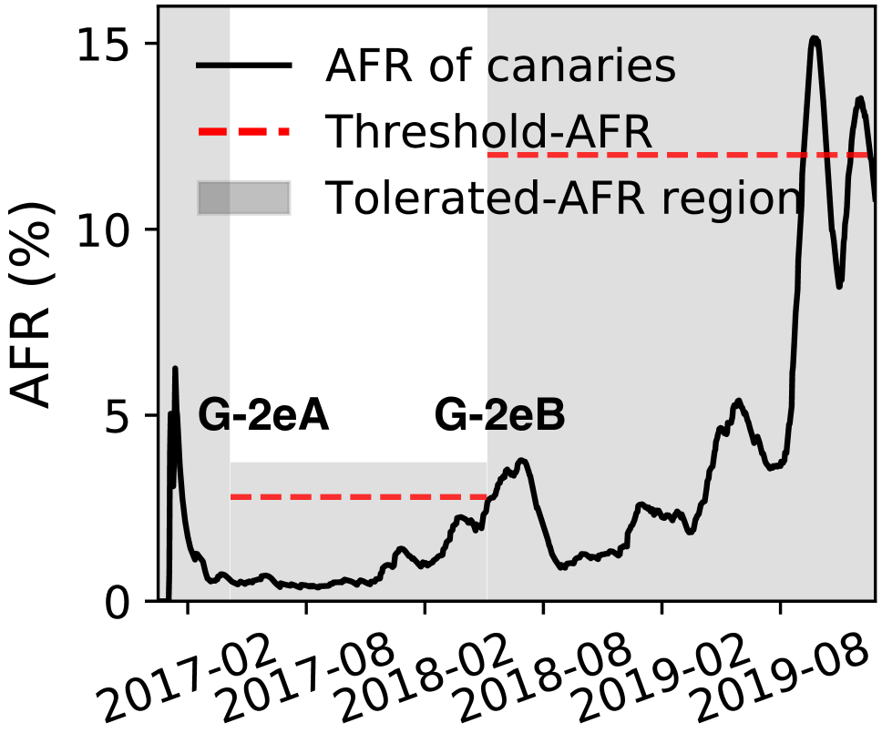
(d) G-2 (trickle) AFR curve

Figure 5: Detailed IO analysis and space savings achieved by pacemaker-enabled adaptive redundancy on Google Cluster1.

pacemaker does not change the file manipulation API or client access paths. But, there is one corner-case related to transitions when file reads can be affected internally. To read a file, a client queries the NN for the inode and caches it. Subsequently, the reads are performed directly from the client to the DN. If the DN transitions to another Rgroup while the file is still being read, the HDFS client may find that that DN no longer has the requested data. But, because this design uses existing HDFS decommissioning for transitions, the client software knows to react by re-requesting the updated inode from the NN and resuming the read.

7 Evaluation

pacemaker-enabled disk-adaptive redundancy using is evaluated on production logs from four large-scale real-world storage clusters, each with hundreds of thousands of disks. We also experiment with a proof-of-concept HDFS implementation on a smaller sized cluster. This evaluation has four primary takeaways: (1) pacemaker eliminates transition overload, never using more than 5% of cluster IO bandwidth (0.2–0.4% on average) and always meets target MTTDL, in stark contrast to prior work approaches that do not account for transition IO load; (2) pacemaker provides more than 97% of idealized-potential space-savings, despite being proactive, reducing disk capacity needed by 14–20% compared to one-size-fits-all; (3) pacemaker’s behavior is not overly sensitive across a range of values for its configurable parameters; (4) pacemaker copes well with the real-world AFR characteristics explained in §3.2. For example, it successfully combines the “multiple useful life phases” observation with efficient transitioning schemes. This evaluation also shows pacemaker in action by measuring disk-adaptive redundancy in pacemaker-enhanced HDFS.

Evaluation methodology. pacemaker is simulated chronologically for each of the four cluster logs described in §3: three clusters from Google and one from Backblaze. For each simulated date, the simulator changes the cluster composition according to the disk additions, failures and decommissioning events in the log. pacemaker is provided the log information, as though it were being captured live in the cluster. IO bandwidth needed for each day’s redundancy management is computed as the sum of IO for failure reconstruction and transition IO requested by pacemaker, and is reported as a fraction of the configured cluster IO bandwidth (100MB/sec per disk, by default).

pacemaker was configured to use a peak-IO-cap of 5%, an average-IO constraint of 1% and a threshold-AFR of 75% of the tolerated-AFR, except for the sensitivity studies in §7.3. For comparison, we also simulate (1) an idealized disk-adaptive redundancy system in which transitions are instantaneous (requiring no IO) and (2) the prior state-of-the-art approach (HeART) for disk-adaptive redundancy. For all cases, Rgroup0 uses 6-of-9, representing a one-size-fits-all scheme reported in prior literature [13]. The required target MTTDL is then back-calculated using the 6-of-9 default and an assumed tolerated-AFR of 16% for Rgroup0. These configuration defaults were set by consulting storage administrators of clusters we evaluated.

7.1 pacemaker on Google Cluster1 in-depth

Fig. 5(a) shows the IO generated by pacemaker (and disk count) over the $\approx$3-year lifetime of Google Cluster1. Over time, the cluster grew to over 350K disks comprising of disks from 7 makes/models (Dgroups) via a mix of trickle and step deployments. Fig. 5(b) and Fig. 5(d) show AFR curves of 2 of the 7 Dgroups (obfuscated as G-1 and G-2 for confidentiality) along with how pacemaker adapted to them at each age. G-1 disks are trickle-deployed whereas G-2 disks are step-deployed. The other 5 Dgroups are omitted due to lack of space. Fig. 5(c) shows the corresponding space-savings (the white space above the colors).

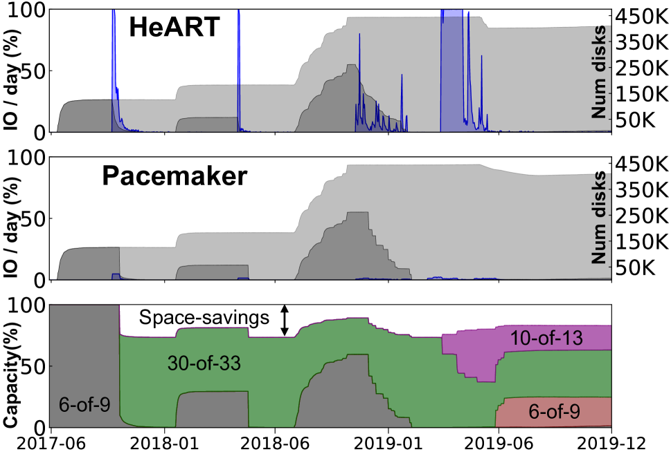
(a) Google Cluster2

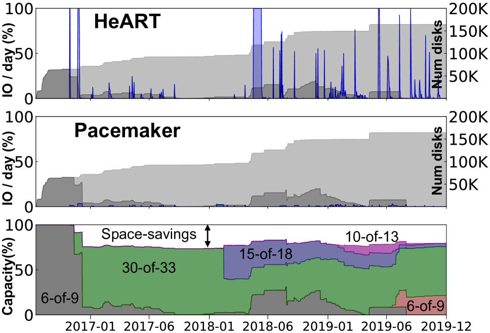
(b) Google Cluster3

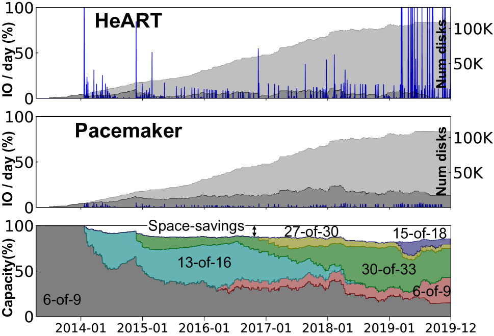
(c) Backblaze

Figure 6: Top two rows show the IO overhead comparison between prior adaptive redundancy system (HeART) and pacemaker on two Google clusters and one Backblaze cluster. pacemaker successfully bounds all IO under 5% (visible as tiny blue regions in middle graphs, for e.g. around 2017 in 6(a)). The bottom row shows the 14–20% average space-savings achieved by pacemaker across the three clusters. The AFR curves of all three clusters are shown in Figs. 10– 12 in Appendix B.

All disks enter the cluster as unspecialized disks, i.e. Rgroup0 (dark gray region in the Fig. 5(a) and left gray region of Figs. 5(b) and 5(d)). Once a Dgroup’s AFR reduces sufficiently, pacemaker RDn transitions them to a specialized Rgroup (light gray area in Fig. 5(a)). Over their lifetime, disks may transition through multiple RUp transitions over the multiple useful life phases. Each transition requires IO, which is captured in blue in Fig. 5(a). For example, the sudden drop in the unspecialized disks, and the blue area around 2018-04 captures the Type 2 transitions caused when over 100K disks RDn transition from Rgroup0 to a specialized Rgroup. The light gray region in Fig. 5(a) corresponds to the time over which space-savings are obtained, which can be seen in Fig. 5(c).

Many transitions with no transition overload. pacemaker successfully bounds all redundancy management IO comfortably under the configured peak-IO-cap throughout the cluster’s lifetime. This can be seen via an imaginary horizontal line at 5% (the configured peak-IO-cap) that none of the blue regions goes above. Recall that pacemaker rate-limits the IO within each Rgroup to ensure simultaneous transitions do not violate the cluster’s IO cap. Events G-1eA and G-2eA are examples of events where both G-1 and G-2 disks (making up almost 100% of the cluster at that time) request transitions at the same time. Despite that, the IO remains bounded below 5%. G-3eC and G-6eB also show huge disk populations of G-3 and G-6 Dgroups (AFRs not shown) requesting almost simultaneous RUp transitions, but pacemaker’s design ensures that the peak-IO constraint is never violated. This is in sharp contrast with HeART’s frequent transition overload, shown in Fig. 1(a).

Disks experience multiple useful life phases. G-1, G-3, G-6 and G-7 disks experience two phases of useful life each. In Fig. 5(a), events G-1eA and G-1eB mark the two transitions of G-1 disks through its multiple useful lives as shown in Fig. 5(b). In the absence of multiple useful life phases, pacemaker would have RUp transitioned G-1 disks to Rgroup0 in 2019-05, eliminating space-savings for the remainder of their time in the cluster. §7.3 quantifies the benefit of multiple useful life phases for all four clusters.

MTTDL always at or above target. Along with the AFR curves, Figs. 5(b) and 5(d) also show the upper bound on the AFR for which the reliability constraint is met (top of the gray region). pacemaker sufficiently protects all disks throughout their life for all Dgroups across evaluated clusters.

Substantial space-savings. pacemaker provides 14% average space-savings (Fig. 5(c)) over the cluster lifetime to date. Except for 2017-01 to 2017-05 and 2017-11 to 2018-03, which correspond to infancy periods for large batches of new empty disks added to the cluster, the entire cluster achieves $\approx$20% space-savings. Note that the apparent reduction in space-savings from 2017-11 to 2018-03 isn’t actually reduced space in absolute terms. Since Fig. 5(c) shows relative space-savings, the over 100K disks deployed around 2017-11, and their infancy period makes the space-savings appear reduced relative to the size of the cluster.

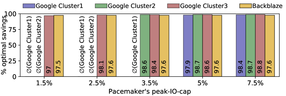
(a) pacemaker’s sensitivity to the peak-IO constraint.

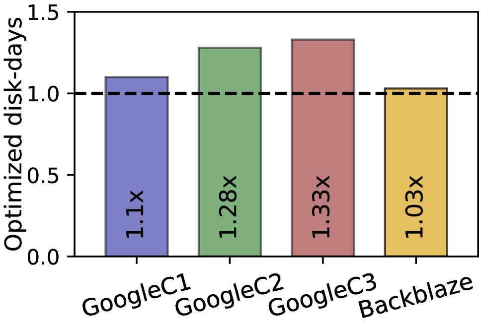
(b) Multiple useful life phases

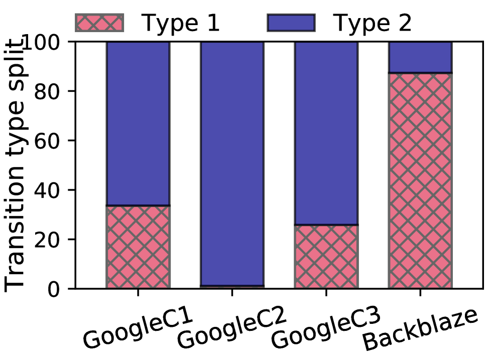
(c) Transition type distribution

Figure 7: 7(a) shows pacemaker’s sensitivity to the peak IO bandwidth constraint. 7(b) shows the advantage of multiple useful life phases and 7(c) shows the contribution of the two transitioning techniques when pacemaker was simulated on the four production clusters.

7.2 pacemaker on the other three clusters

Fig. 6 compares the transition IO incurred by pacemaker to that for HeART [26] for Google Cluster2, Google Cluster3 and Backblaze, along with the corresponding space-savings achieved by pacemaker. While clusters using HeART would suffer transition overload, the same clusters under pacemaker always had all their transition IO under the peak-IO-cap of 5%. In fact, on average, only 0.21–0.32% percent of the cluster IO bandwidth was used for transitions. The average space-savings for the three clusters are 14–20%.

Google Cluster2. Fig. 6(a) shows the transition overload and space-savings in Google Cluster2 and the corresponding space-savings. All Dgroups in Google Cluster2 are step-deployed. Thus, it is not surprising that Fig. 7(c) shows that over 98% of the transitions in Cluster2 were Type 2 transitions (bulk parity recalculation). Cluster2’s disk population exceeds 450K disks. Even at such large scales, pacemaker obtains average space-savings of almost 17% and peak space-savings of over 25%. This translates to needing 100K fewer disks.

Google Cluster3. Google Cluster3 (Fig. 6(b)) is not as large as Cluster1 or Cluster2. At its peak, Cluster3 has a disk population of approximately 200K disks. But, it achieves the highest average space-savings (20%) among clusters evaluated. Like Cluster2, Cluster3 is also mostly step-deployed.

Backblaze Cluster. Backblaze (Fig. 6(c)) is a completely trickle-deployed cluster. The dark grey region across the bottom of Fig. 6(c)’s pacemaker plot shows the persistent presence of canary disks throughout the cluster’s lifetime. Unlike the Google clusters, the transition IO of Backblaze does not produce bursts of transition IO that lasts for weeks. Instead, since trickle-deployed disks transition a-few-at-a-time, we see transition work appearing continuously throughout the cluster lifetime of over 6 years. The rise in the transition IO spikes in 2019, for HeART, is because of large capacity 12TB disks replacing 4TB disks. Unsurprisingly, under pacemaker, most of the transitions are done using Type 1 (transitioning by emptying disks) as shown in Fig. 7(c). The average space-savings obtained on Backblaze are 14%.

7.3 Sensitivity analyses and ablation studies

Sensitivity to IO constraints. The peak-IO constraint governs Fig. 7(a), which shows the percentages of optimal space-savings achieved with pacemaker for peak-IO-cap settings between 1.5% and 7.5%. A peak-IO-cap of up to 7.5% is used in order to compare with the IO percentage spent for existing background IO activity, such as scrubbing. By scrubbing all data once every 15 days [5], the scrubber uses around 7% IO bandwidth, and is a background work IO level tolerated by today’s clusters.

The Y-axis captures how close the space-savings are for the different peak-IO-caps compared to “Optimal savings”, i.e. an idealized system with infinitely fast transitions. pacemaker’s default peak-IO-cap (5%) achieves over 97% of the optimal space-savings for each of the four clusters. For peak-IO constraint set to $<=$2.5%, some RUp transitions in Google Cluster1 and Cluster2 become too aggressively rate-limited causing a subsequent AFR rise to violate the peak-IO constraints. We indicate this as a failure, and show it as "$\varnothing$". The same situation happens for Google Cluster1 at 3.5%.

Sensitivity to threshold-AFR. The threshold-AFR determines when proactive RUp transitions of step-deployed disks are initiated. Conceptually, the threshold-AFR governs how risk-averse the admin wants to be. Lowering the threshold would trigger an RUp transition when disks are farther away from the tolerated-AFR (more risk-averse), and vice-versa. We evaluated pacemaker for threshold-AFRs of 60%, 75% and 90% of the respective Rgroups’ tolerated-AFRs. We found that pacemaker’s space-savings is not very sensitive to threshold-AFR, with space-savings only 2% lower at 60% than at 90%. Data remained safe at each of these settings, but would become unsafe with higher values.

Contribution of multiple useful life phases. Fig. 7(b) compares the increased number of disk-days spent in specialized Rgroups because of considering multiple useful life phases. In the best case, Google Cluster2 spent 33% more disk-days in specialized redundancy, increasing overall space-savings from 16% to 19%. Note that in large-scale storage clusters, even 1% space-savings are considered substantial as it represents thousands of disks.

Contribution of transition types. By proactively keeping step-deployed disks in distinct Rgroups and using specialized transitioning schemes whenever possible, instead of using simple re-encoding for all transitions, pacemaker reduces total transition IO by 92–96% for the four clusters. Fig. 7(c) shows what percentage of transitions were done via Type 1 (disk emptying) vs. Type 2 (bulk parity recalculation). As expected, Google clusters rely more on Type 2 transitions, because most disks are step-deployed. In contrast, the Backblaze cluster is entirely trickle-deployed and hence mostly uses Type 1 transitions. The small percentage of Type 2 transitions in Backblaze occur when Rgroups are purged.

7.4 Evaluating HDFS + pacemaker

This section describes basic experiments with the pacemaker-enabled HDFS, focusing on its functioning and operation. Note that pacemaker is designed for longitudinal disk deployments over several years, a scenario that cannot be reproduced identically in laboratory settings. Hence, these HDFS experiments are aimed to display that integrating pacemaker with an existing storage system is straightforward, rather than on the long-term aspects like overall space-savings or transition IO behavior over cluster lifetime as evaluated via simulation above.

The HDFS experiments run on a PRObE Emulab cluster [16]. Each machine has a Dual-Core AMD Opteron Processor, 16GB RAM, and Gigabit Ethernet. We use a 21-node cluster running HDFS 3.2.0 with one NN and 20 DNs. Each DN has a 10GB partition on a 10000 RPM HDD for a total cluster size of 200GB. We statically define the cluster to be made up of two Rgroups of ten DNs each, one using the 6-of-9 erasure coding scheme and the other using a 7-of-10 scheme. DFS-perf [19], a popular open-source HDFS benchmark is used, after populating the cluster to 60% full. Each DFS-perf client sequentially reads one file over and over again (size=768MB), for a total read size of about 1.75TB over 40 iterations. We use 60 DFS-perf clients, running on 20 nodes separate from the HDFS cluster.

We focus on the behavior of a DN as it transitions between Rgroups, compared with baseline HDFS performance (where all DNs are healthy) and its behavior while recovering from a failed DN. Fig. 8 shows the client throughput after the setup phase, followed by a noticeable drop in client throughput when a DN fails (emuated by stopping the DN). This is caused by the reconstruction IO that recreates the data from the failed node. Read latency exhibits similar behavior (not shown due to space). Eventually, throughput settles at about 5% lower than prior to failure, since now there are 19 DNs.

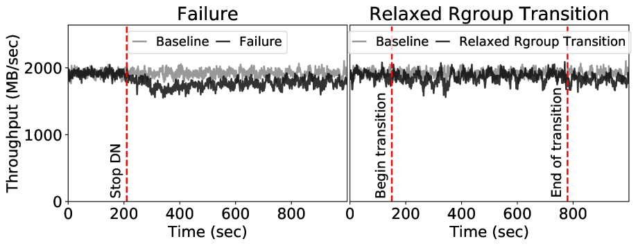
Figure 8: DFS-perf reported throughput for baseline, with one DN failure and one Rgroup transition.

Fig. 8 also shows client throughput when a node is RDn transitioned from 6-of-9 to 7-of-10. There is minor interference during the transition, which can be attributed to the data movement that HDFS performs as a part of decommissioning. The transition requires less work than failed node reconstruction, yet takes longer to complete because pacemaker limits the transition IO. Eventually, even though 20 DNs are running, the throughput is lower by $\approx$5% (one DN’s throughput). This happens because pacemaker empties the DN before it moves into the new Rgroup, and load-balancing data to newly added DNs happens over a longer time-frame. Experiments with RUp transition showed similar results.

8 Related work

The closest related work [26] proposes a redundancy adaptation tool called HeART that categorizes disks into groups and suggests a tailored redundancy scheme for each during its useful life period. As discussed earlier, while [26] showcased potential space-savings, it ignored transition overload and hence is made impractical (Fig. 1(a)). pacemaker eliminates transition overload by employing IO constraints (specifically the peak-IO and average-IO constraints) that cap the transition IO to a tiny fraction cluster bandwidth. While HeART was evaluated only for the trickle-deployed Backblaze cluster, our evaluation of pacemaker for Google storage clusters exposes the unique challenges of step-deployed clusters. Several design elements were added to pacemaker to address the challenges posed by step-deployed disks.

Various systems include support for multiple redundancy schemes, allowing different schemes to be used for different data [14, 12]. Tools have been created for deciding, on a per-data basis, which scheme to use [66, 59]. Keeton et al. [27] describe a tool that automatically provides disaster-resistant solutions based on budget and failure models. pacemaker differs from such systems by focusing on efficiently adapting redundancy to different and time-varying AFRs of disks.

Reducing the impact of background IO, such as for data scrubbing, on foreground IO is a common research theme. [1, 3, 30, 29, 37, 52]. pacemaker converts otherwise-urgent bursts of transition IO into proactive background IO, which could then benefit from these works.

Disk reliability has been well studied, including evidence of failure rates being make/model dependent [5, 11, 22, 25, 31, 39, 40, 48, 49, 50, 54]. There are also studies that predict disk failures [2, 20, 32, 36, 57, 62, 69], which can enhance any storage fault-tolerance approach.

While several works have considered the problem of designing erasure codes that allow transitions using less resources, existing solutions are limited to specific kinds of transitions and hence are not applicable in general. The case of adding parity chunks while keeping the number of data chunks fixed can be viewed [44, 46, 34] as the well-studied reconstruction problem, and hence the codes designed for optimal reconstruction (e.g., [10, 45, 46, 61, 18, 38]) would lead to improved resource usage for this case. Several works have studied the case where the number of data nodes increases while the number of parity nodes remains fixed [70, 65, 67, 23, 41]. In [66], the authors propose two erasure codes designed to undergo a specific transition in parameters. In [33], the authors propose a general theoretical framework for studying codes that enable efficient transitions for general parameters, and derive lower bounds on the cost of transitions as well as describe optimal code constructions for certain specific parameters. However, none of the existing code constructions are applicable for the diverse set of transitions needed for disk-adaptive redundancy in real-world storage clusters.

9 Conclusion

pacemaker orchestrates disk-adaptive redundancy without transition overload, allowing use in real-world clusters. By proactively arranging data layouts and initiating transitions, pacemaker reduces total transition IO allowing it to be rate-limited. Its design integrates cleanly into existing scalable storage implementations, such as HDFS. Analysis for 4 large real-world storage clusters from Google and Backblaze show 14–20% average space-savings while transition IO is kept small ($<$0.4% on average) and bounded (e.g., $<$5%).

10 Acknowledgements

We thank our shepherd Wyatt Lloyd and the anonymous reviewers for their valuable feedback and suggestions. We extend special thanks to Larry Greenfield, Arif Merchant and numerous other researchers, engineers at Google; Keith Smith, Tim Emami, Jason Hennessey, Peter Macko and other researchers from NetApp’s Advanced Technology Group (ATG) who have been instrumental in providing data, feedback and support. We also thank Jiaan Dai, Xuren Zhou, Jiaqi Zuo, Sai Kiriti Badam and Jiongtao Ye for their help in building the HDFS+pacemaker prototype. This research is generously supported in part by the NSF grants CNS 1956271 and CNS 1901410. We also thank the members and companies of the PDL Consortium (Alibaba, Amazon, Datrium, Facebook, Google, HPE, Hitachi, IBM, Intel, Microsoft, NetApp, Oracle, Pure Storage, Salesforce, Samsung, Seagate, Two Sigma, Western Digital) and VMware for their interest, insights, feedback, and support.

Appendix A Failure rate estimation details

This section describes how we calculate failure rates for each Dgroup based on the disks’ age using empirical data. In the storage device reliability literature, the failure rate over a period of time is typically expressed in terms of Annualized Failure Rate (AFR), and calculated as:

$$AFR\ (\%)=\frac{d}{E}\times 100,$$ (1)

where $d$ is the number of observed disk failures, and $E$ is the sum of the exposure time of each disk, measured in years. The exposure time of a disk is the amount of time it was in operation (i.e., deployed and had not failed nor been retired) during the period in consideration, and it is typically measured at the granularity of days.

If the time to failure is exponentially distributed, then Formula 1 corresponds to the maximum likelihood estimate for the rate parameter of the exponential distribution. Due to the memoryless property of this distribution, such a formula would be appropriate only if we assume that failure rate is constant with respect to time or device age. Thus, Eq. 1 may be useful for estimating AFR over long and stable periods of time, but makes it hard to reason about changes in AFR over time. Therefore, in this work, we estimate AFR using the following approach.

Assume that the lifetime (time from deployment to failure) of each disk is an i.i.d. discrete random variable $T$ with cumulative density function $F$ and probability mass function $f$. The failure rate (also known as hazard rate) [60] of this distribution is given by:

$$h(t)=f(t)/(1-F(t)).$$ (2)

The cumulative hazard defined as $H(t)=\sum_{i=0}^{t}h(i)$ is commonly estimated using the Nelson-Aalen estimator:

$$\hat{H}(t)=\sum_{i=0}^{t}\frac{d_{i}}{a_{i}}\qquad\text{for }t\in\{0,\ldots,m\},$$ (3)

where $d_{i}$ is the number of disks that failed during their $i$-th day, $a_{i}$ is the number of disks that were in operation at the start of their $i$-th day, and $m$ is the age in days of the oldest observed disk drive. An estimate for the failure rate can be obtained by applying the so-called kernel method [58]:

$$\hat{h}(t)=\sum_{i=0}^{m}\frac{d_{i}}{a_{i}}K(t-i),\qquad\text{for }t\in\{0,\ldots,m\},$$ (4)

where $K(\cdot)$ is a kernel function. In practice, Formula 4 can be considered as a smoothing over the increments of Formula 3. For our calculations, we utilized an Epanechnikov kernel [21] with a bandwidth of 30 days (the Epanechnikov kernel is frequently used in practice due to its good theoretical properties).

A big advantage of this approach is that it is nonparametric, meaning that it does not assume that the lifetime $T$ follows any particular distribution. This allows pacemaker to adapt and work effectively with a wide arrange of storage devices with vastly different failure rate behaviors.

Appendix B Detailed cluster evaluations

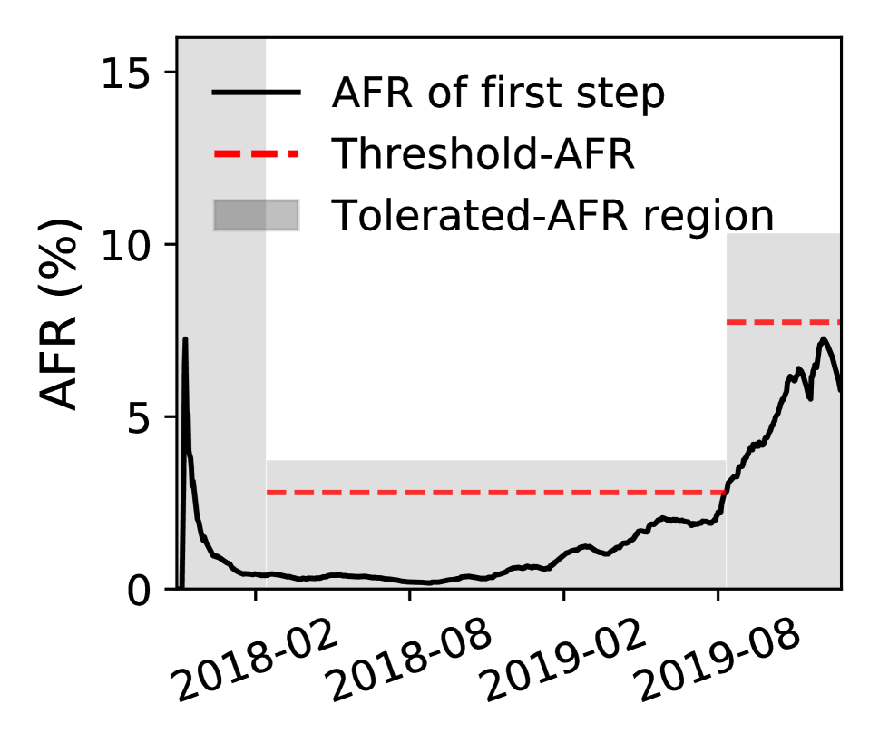
(a) G-6 (step) AFR curve

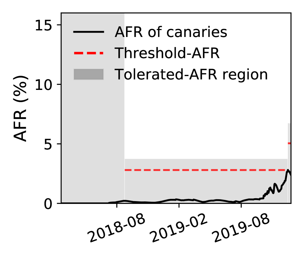
(b) G-4 (trickle) AFR curve

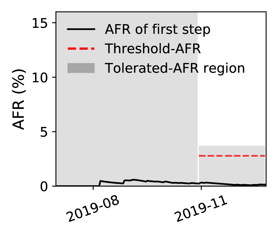
(c) G-8 (step) AFR curve

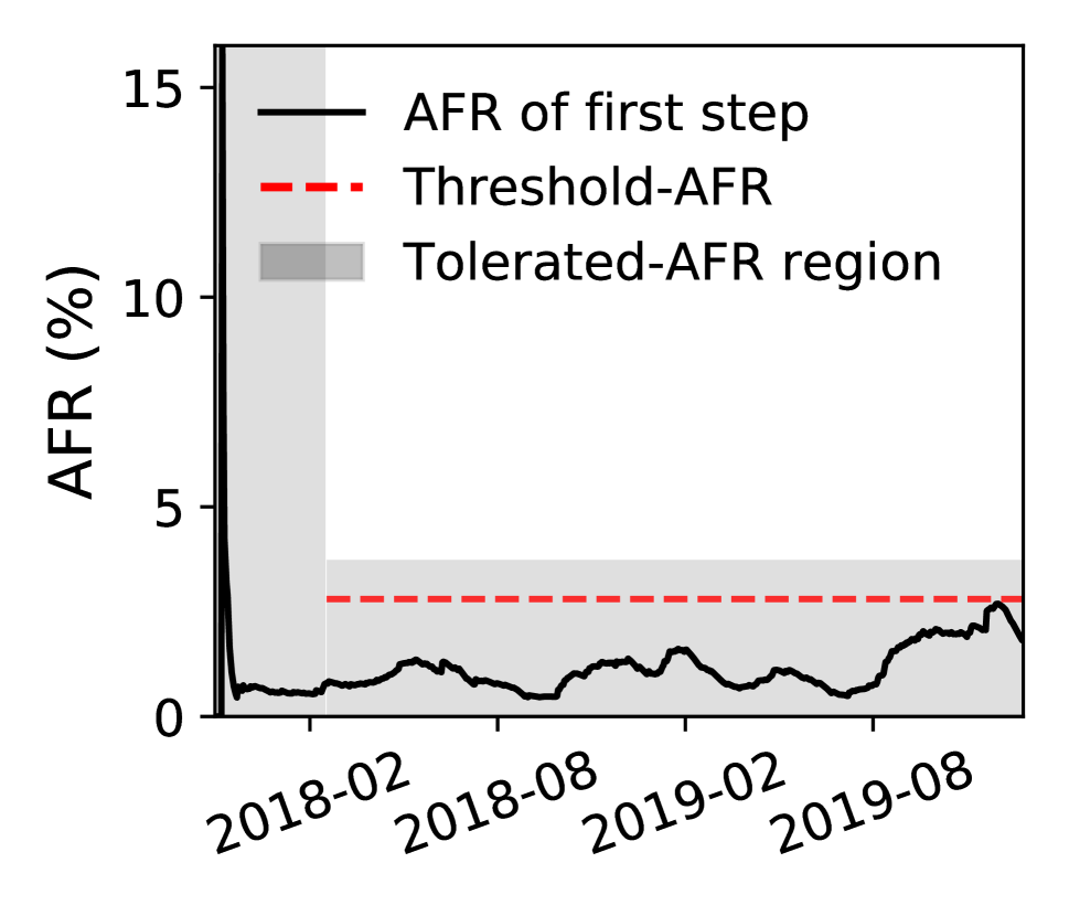
(d) G-5 (step) AFR curve

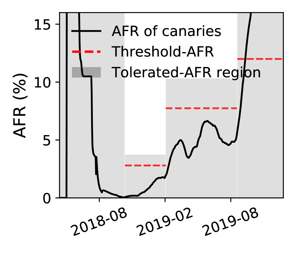
(e) G-3 (trickle) AFR curve

Figure 9: Detailed IO analysis and space savings achieved by pacemaker-enabled adaptive redundancy on Google Cluster1.

This section shows the remaining Dgroups of Google Cluster1 (Fig. 9) and provides a similar deep-dive of pacemaker on Google Cluster2, Google Cluster3 and the Backblaze cluster along with the AFR curves of all Dgroups of those clusters.

Dgroups of Google Cluster1. Recall from §7 that Google Cluster1 is made up of seven Dgroups. G-1 and G-2 AFR curves are shown in Figs. 5(b) and 5(d) respectively. Here we show the four of the file remaining Dgroups, viz. G-3, G-5, G-6 and G-7 in Figs. 9(a)–9(e). G-3 and G-7 disks are trickle-deployed similar to G-2 disks, whereas the other disks are step-deployed.

Google Cluster2. Fig. 10(a) shows the pacemaker-generated IO for redundancy management. Fig. 10(b) shows the corresponding space savings. Finally Figs. 10(c)–10(f) shows the AFRs of the four Dgroups that make up Cluster2. All Dgroups in Google Cluster2 are step-deployed. Thus, it is not surprising that Fig. 7(c) shows that over 98% of the transitions in Cluster2 were performed by bulk parity recalculation. This is the largest cluster pacemaker was simulated on. Cluster2’s disk population exceeds 450K disks. Even at such large scales, pacemaker is able to obtain average space savings of almost 17% and peak space savings of over 25%. This translates to needing 100K fewer disks, essentially saving millions of dollars.

Google Cluster3. Google Cluster3 is not as large as Cluster1 or Cluster2. At its peak, Cluster3 has a disk population of approximately 200K disks. But, it achieves the highest average space savings (20%) compared to all other clusters. Fig. 11(a) shows the pacemaker-generated IO, Fig, 11(b) shows the space savings and Figs. 11(c)–11(e) shows the AFR curves of its three Dgroups. Like Cluster2, Cluster3 is also mostly step-deployed.

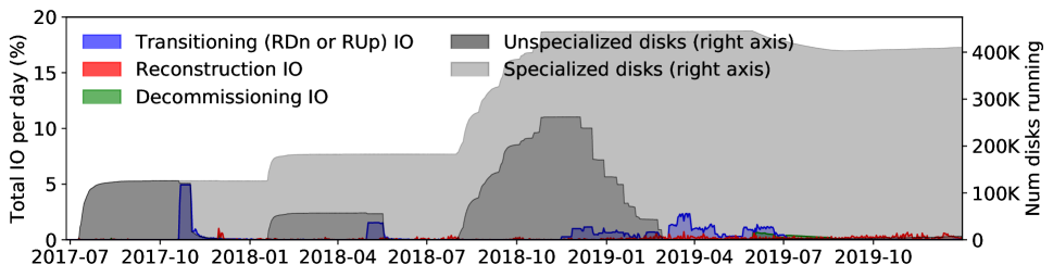
(a) Google Cluster2 redundancy management IO due to pacemaker over its 2$+$ year lifetime broken down by IO type.

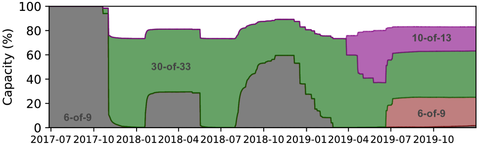
(b) Google Cluster2 space savings achieved by pacemaker.

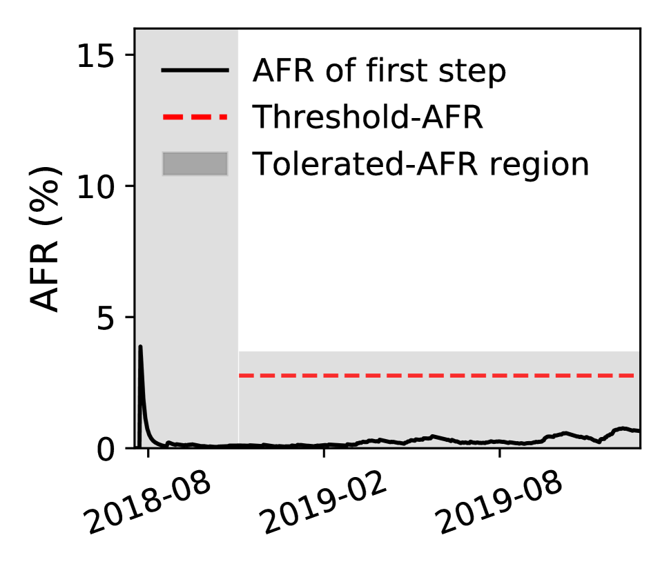
(c) G-6 (step) AFR curve

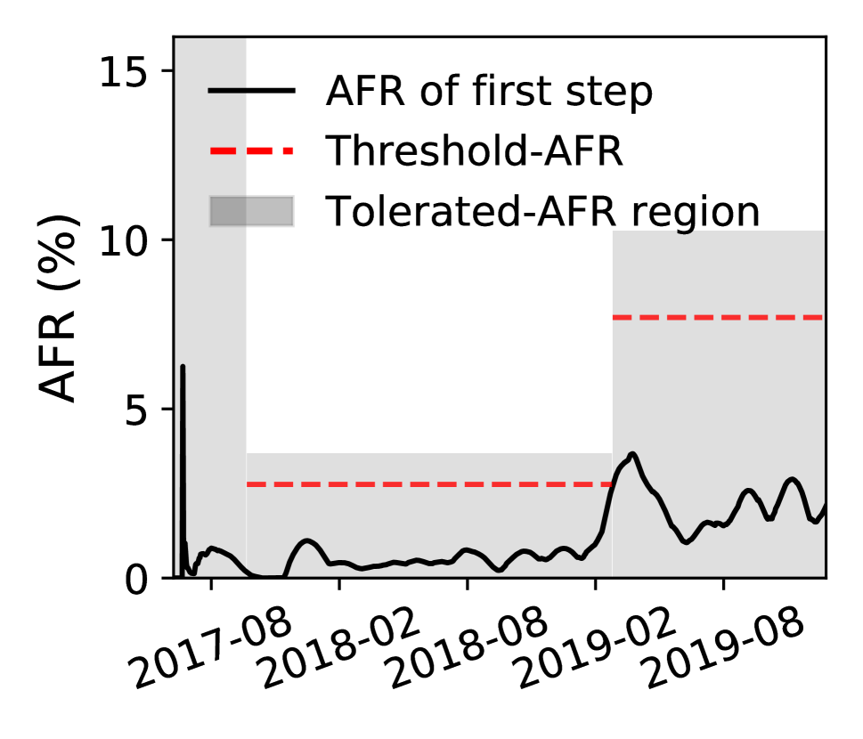
(d) G-1 (step) AFR curve

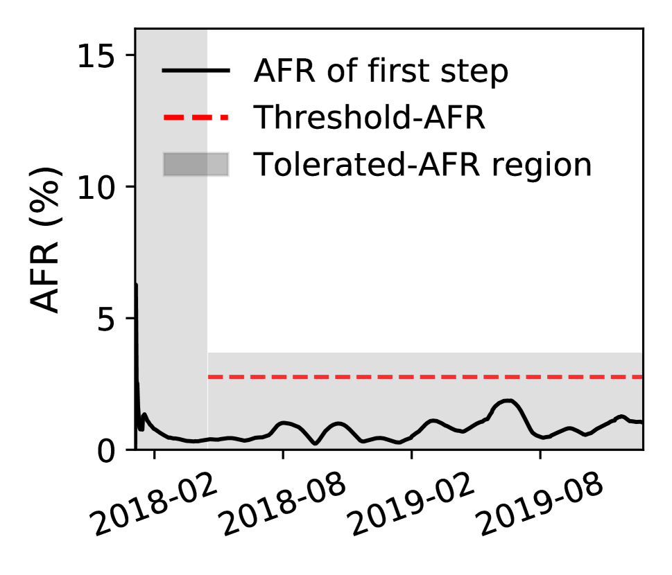
(e) G-5 (step) AFR curve

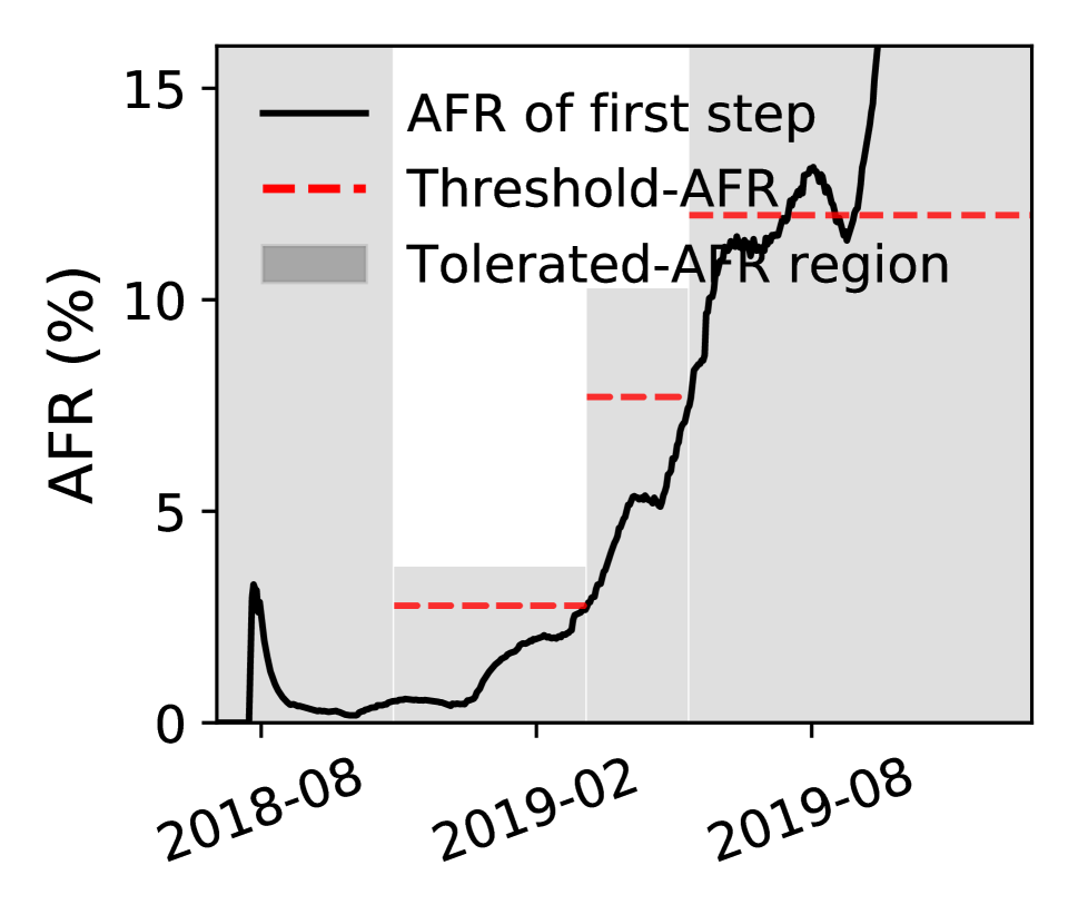
(f) G-3 (step) AFR curve

Figure 10: Detailed IO analysis and space savings achieved by pacemaker-enabled adaptive redundancy on Google Cluster2.

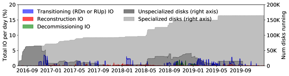
(a) Google Cluster3 redundancy management IO due to pacemaker over its 3 year lifetime broken down by IO type.

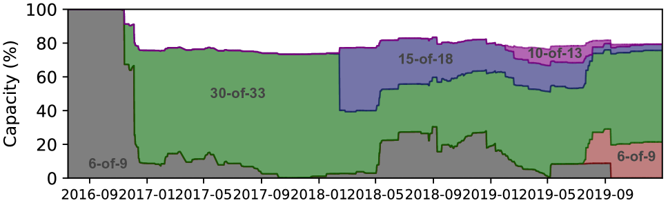
(b) Google Cluster3 space savings achieved by pacemaker.

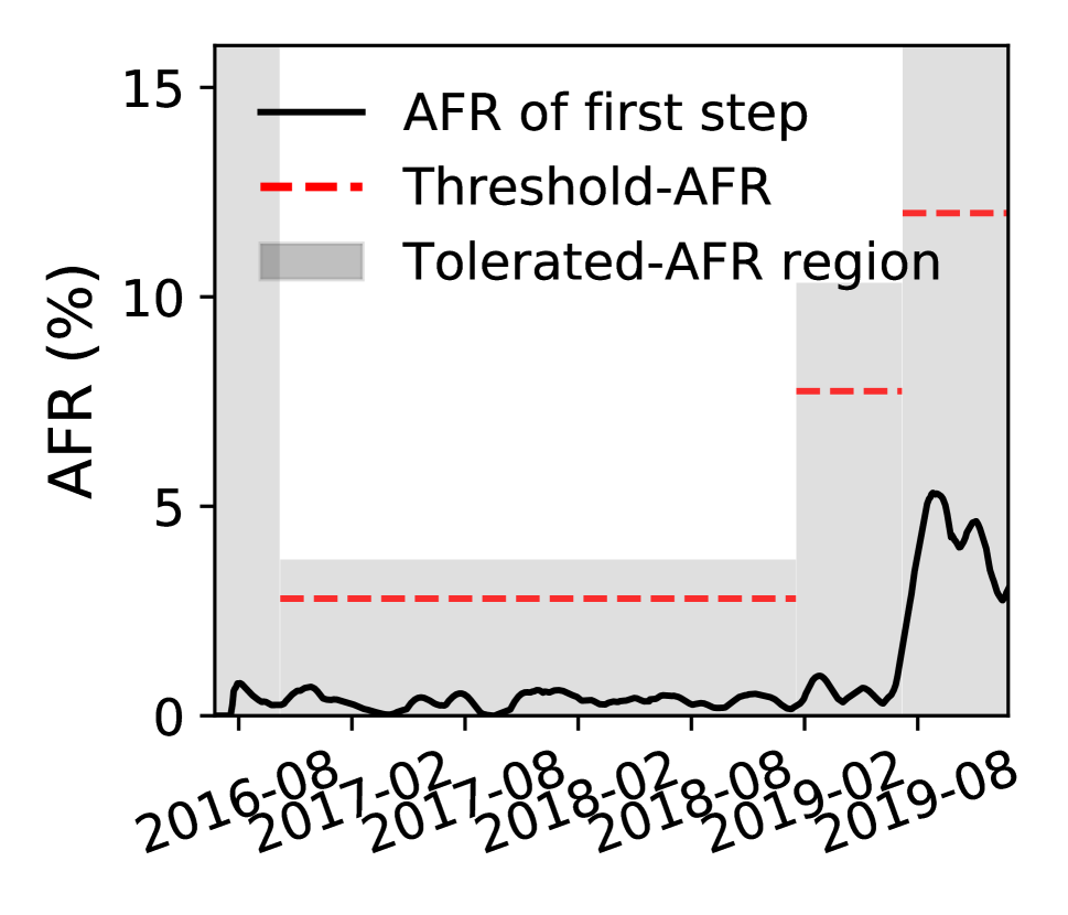
(c) G-2 (step) AFR curve

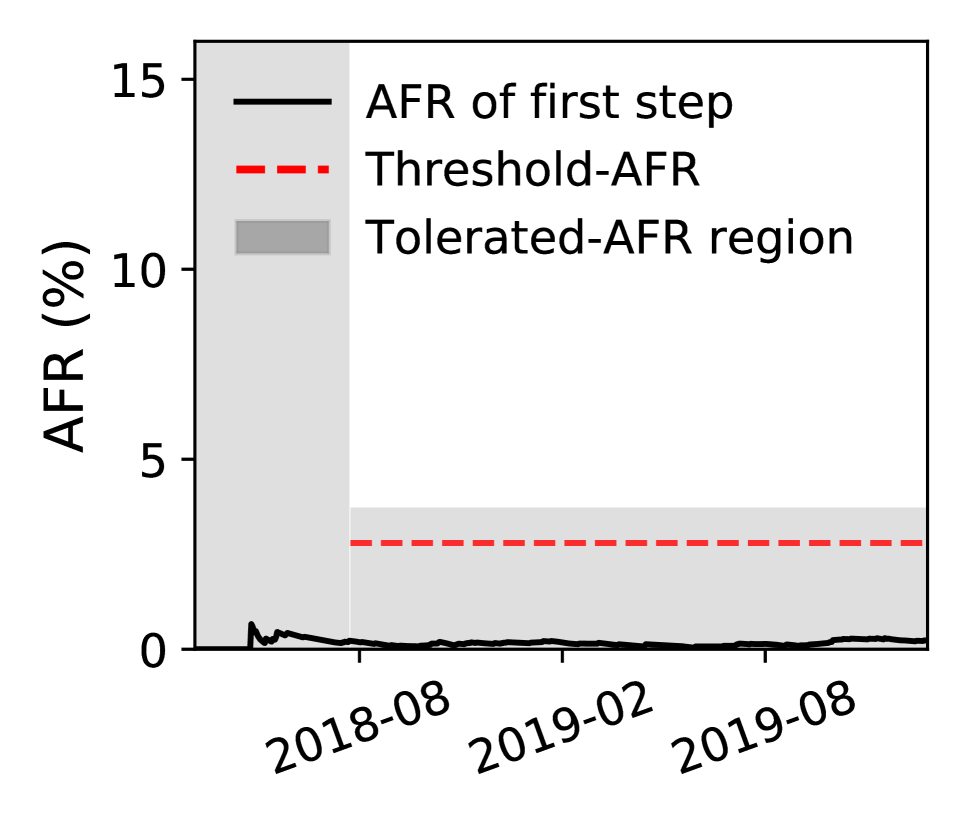
(d) G-4 (step) AFR curve

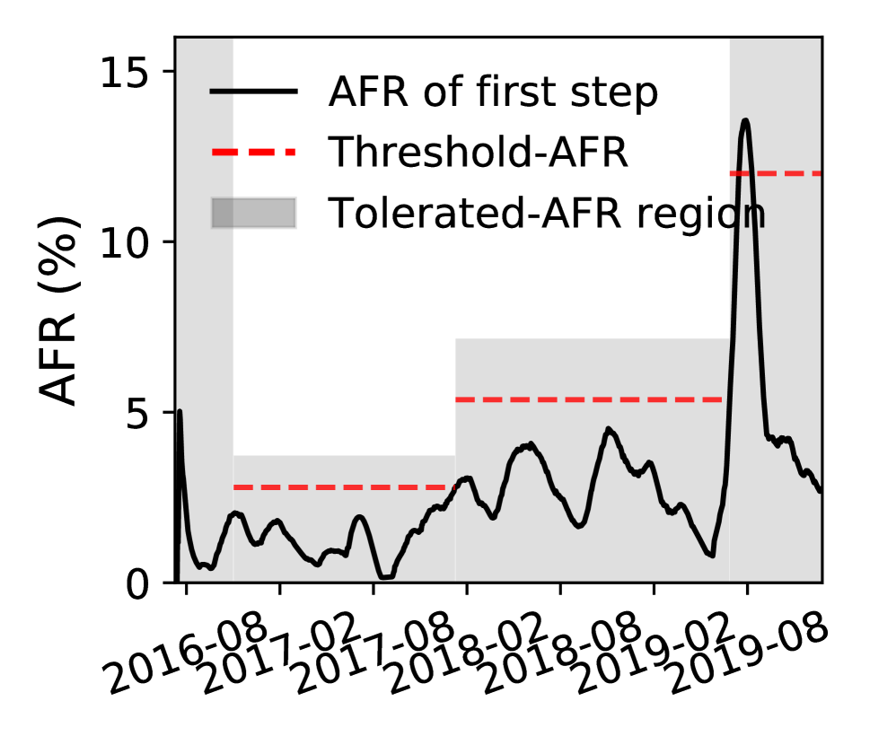
(e) G-1 (step) AFR curve

Figure 11: Detailed IO analysis and space savings achieved by pacemaker-enabled adaptive redundancy on Google Cluster3.

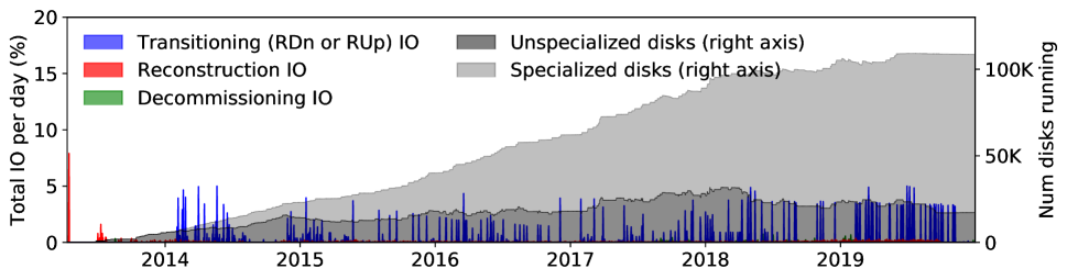
(a) Backblaze redundancy management IO due to pacemaker over its 6$+$ year lifetime broken down by IO type.

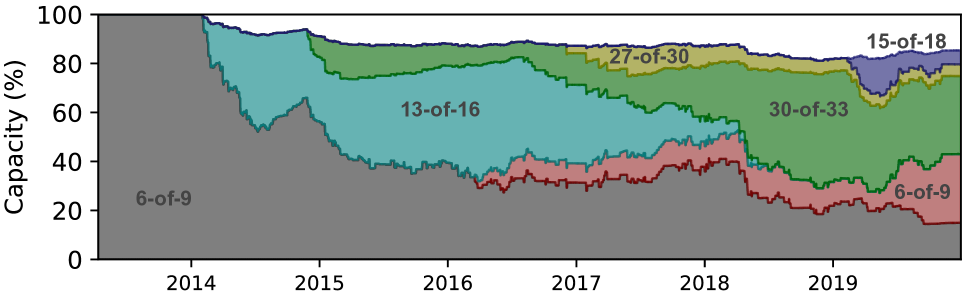
(b) Backblaze space savings achieved by pacemaker.

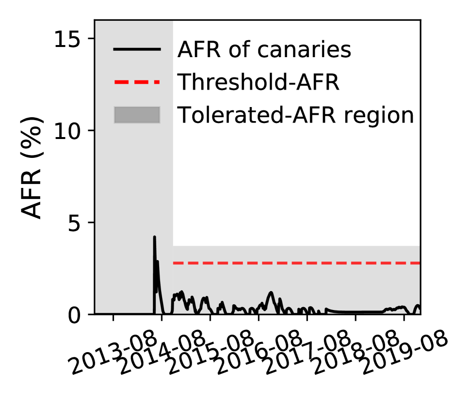
(c) H-4A (trickle) AFR curve

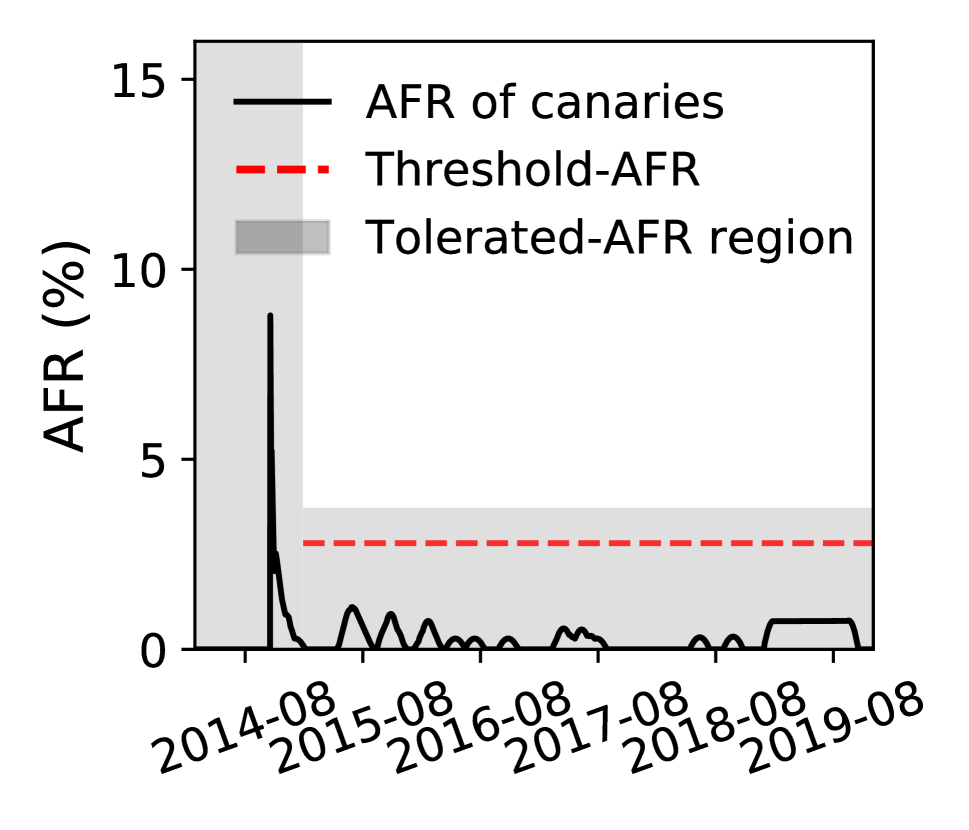
(d) H-4B (trickle) AFR curve

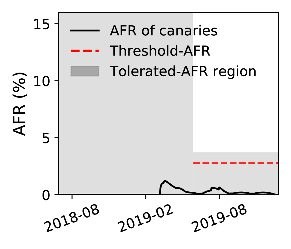
(e) H-12E (trickle) AFR curve

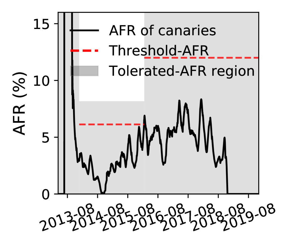
(f) S-4 (trickle) AFR curve

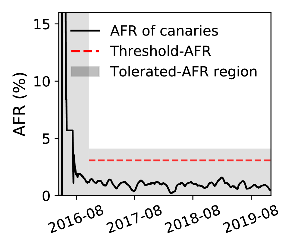
(g) S-8C (trickle) AFR curve

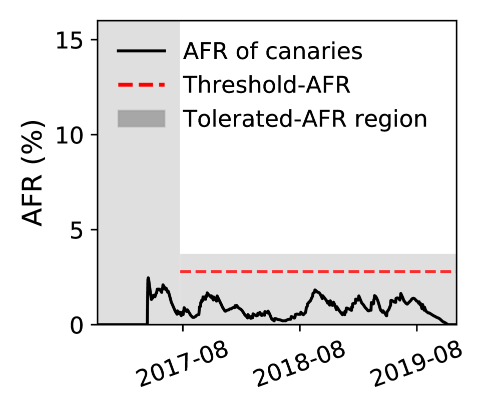
(h) S-8E (trickle) AFR curve

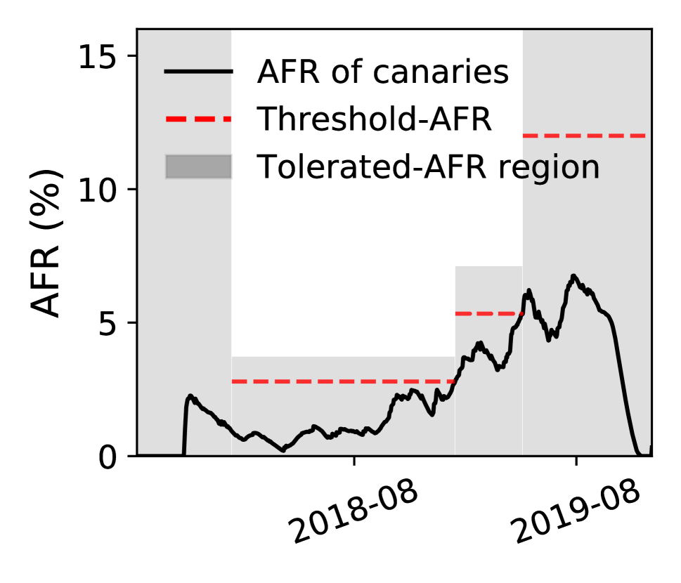
(i) S-12E (trickle) AFR curve

Figure 12: Detailed IO analysis and space savings achieved by pacemaker-enabled adaptive redundancy on the Backblaze cluster.

Backblaze Cluster. Backblaze is a completely trickle-deployed cluster. Fig. 12(a) shows the pacemaker-generated IO. Unlike Google clusters, the transition IO of Backblaze does not produce large regions of transition workload. Instead, since trickle-deployed disks transition a-few-at-a-time, we see transition work appearing continuously throughout the cluster lifetime of over 6 years. Unsurprisingly, most of the transitions are done by emptying disks (Type 1; refer Fig. 7(c)). In terms of sensitivity, the Backblaze cluster is the most insensitive to the peak-IO constraint since always requires much lower transition bandwidth per day.

References

- [1] George Amvrosiadis, Angela Demke Brown, and Ashvin Goel. Opportunistic storage maintenance. In ACM Symposium on Operating Systems Principles (SOSP), 2015.
- [2] Preethi Anantharaman, Mu Qiao, and Divyesh Jadav. Large Scale Predictive Analytics for Hard Disk Remaining Useful Life Estimation. In IEEE International Conference on Big Data, 2018.
- [3] Eitan Bachmat and Jiri Schindler. Analysis of methods for scheduling low priority disk drive tasks. In ACM SIGMETRICS Performance Evaluation Review, 2002.
- [4] Backblaze. Disk Reliability Dataset. https://www.backblaze.com/b2/hard-drive-test-data.html, 2013-2018.
- [5] Lakshmi N Bairavasundaram, Garth R Goodson, Shankar Pasupathy, and Jiri Schindler. An analysis of latent sector errors in disk drives. In ACM SIGMETRICS Performance Evaluation Review, 2007.
- [6] Eric Brewer. Spinning Disks and Their Cloudy Future. https://www.usenix.org/node/194391, 2018.
- [7] Eric Brewer, Lawrence Ying, Lawrence Greenfield, Robert Cypher, and Theodore T’so. Disks for data centers. Technical report, Google, 2016.
- [8] Brad Calder, Ju Wang, Aaron Ogus, Niranjan Nilakantan, Arild Skjolsvold, Sam McKelvie, Yikang Xu, Shashwat Srivastav, Jiesheng Wu, Huseyin Simitci, et al. Windows azure storage: a highly available cloud storage service with strong consistency. In ACM Symposium on Operating Systems Principles (SOSP), 2011.
- [9] Byung-Gon Chun, Frank Dabek, Andreas Haeberlen, Emil Sit, Hakim Weatherspoon, M Frans Kaashoek, John Kubiatowicz, and Robert Morris. Efficient Replica Maintenance for Distributed Storage Systems. In USENIX Symposium on Networked Systems Design and Implementation (NSDI), 2006.
- [10] Alexandros G. Dimakis, Brighten Godfrey, Yunnan Wu, Martin J. Wainwright, and Kannan Ramchandran. Network coding for distributed storage systems. IEEE Transactions on Information Theory, 2010.
- [11] Jon Elerath. Hard-disk drives: The good, the bad, and the ugly. Communication of ACM, 2009.
- [12] Erasure code Ceph Documentation. https://docs.ceph.com/docs/master/rados/operations/erasure-code/, (accessed September 25, 2019).
- [13] Daniel Ford, François Labelle, Florentina I Popovici, Murray Stokely, Van-Anh Truong, Luiz Barroso, Carrie Grimes, and Sean Quinlan. Availability in Globally Distributed Storage Systems. In USENIX Symposium on Operating Systems Design and Implementation (OSDI), 2010.
- [14] Apache Software Foundation. HDFS Erasure Coding. https://hadoop.apache.org/docs/r3.0.0/hadoop-project-dist/hadoop-hdfs/HDFSErasureCoding.html, 2017 (accessed November 5, 2020).
- [15] S. Ghemawat, H. Gobioff, and S.T. Leung. The Google file system. In ACM SIGOPS Operating Systems Review, 2003.
- [16] Garth Gibson, Gary Grider, Andree Jacobson, and Wyatt Lloyd. Probe: A thousand-node experimental cluster for computer systems research. USENIX; login, 2013.
- [17] Garth A Gibson. Redundant disk arrays: Reliable, parallel secondary storage. The MIT Press, 1992.
- [18] Parikshit Gopalan, Cheng Huang, Huseyin Simitci, and Sergey Yekhanin. On the locality of codeword symbols. IEEE Transactions on Information Theory, 2012.
- [19] Rong Gu, Qianhao Dong, Haoyuan Li, Joseph Gonzalez, Zhao Zhang, Shuai Wang, Yihua Huang, Scott Shenker, Ion Stoica, and Patrick PC Lee. DFS-PERF: A scalable and unified benchmarking framework for distributed file systems. EECS Dept., Univ. California, Berkeley, Berkeley, CA, USA, Tech. Rep. UCB/EECS-2016-133, 2016.
- [20] Greg Hamerly, Charles Elkan, et al. Bayesian approaches to failure prediction for disk drives. In International Conference on Machine Learning (ICML), 2001.
- [21] Trevor Hastie, Robert Tibshirani, and Jerome Friedman. Kernel smoothing methods. In The elements of statistical learning. Springer, 2009.
- [22] Eric Heien, Derrick Kondo, Ana Gainaru, Dan LaPine, Bill Kramer, and Franck Cappello. Modeling and tolerating heterogeneous failures in large parallel systems. In ACM / IEEE High Performance Computing Networking, Storage and Analysis (SC), 2011.
- [23] Yuchong Hu, Xiaoyang Zhang, Patrick P. C. Lee, and Pan Zhou. Generalized optimal storage scaling via network coding. In IEEE International Symposium on Information Theory (ISIT), 2018.
- [24] Cheng Huang, Huseyin Simitci, Yikang Xu, Aaron Ogus, Brad Calder, Parikshit Gopalan, Jin Li, Sergey Yekhanin, et al. Erasure Coding in Windows Azure Storage. In USENIX Annual Technical Conference (ATC), 2012.
- [25] Weihang Jiang, Chongfeng Hu, Yuanyuan Zhou, and Arkady Kanevsky. Are disks the dominant contributor for storage failures?: A comprehensive study of storage subsystem failure characteristics. ACM Transactions on Storage (TOS), 2008.
- [26] Saurabh Kadekodi, K V Rashmi, and Gregory R Ganger. Cluster storage systems gotta have HeART: improving storage efficiency by exploiting disk-reliability heterogeneity. In USENIX File and Storage Technologies (FAST), 2019.
- [27] Kimberly Keeton, Cipriano A Santos, Dirk Beyer, Jeffrey S Chase, John Wilkes, et al. Designing for disasters. In USENIX File and Storage Technologies (FAST), 2004.
- [28] Larry Lancaster and Alan Rowe. Measuring real-world data availability. 2001.
- [29] Christopher R Lumb, Jiri Schindler, Gregory R Ganger, et al. Freeblock scheduling outside of disk firmware. In USENIX File and Storage Technologies (FAST), 2002.
- [30] Christopher R Lumb, Jiri Schindler, Gregory R Ganger, David F Nagle, and Erik Riedel. Towards higher disk head utilization: extracting free bandwidth from busy disk drives. In USENIX Symposium on Operating Systems Design and Implementation (OSDI), 2000.
- [31] Ao Ma, Rachel Traylor, Fred Douglis, Mark Chamness, Guanlin Lu, Darren Sawyer, Surendar Chandra, and Windsor Hsu. RAIDShield: characterizing, monitoring, and proactively protecting against disk failures. ACM Transactions on Storage (TOS), 2015.
- [32] Farzaneh Mahdisoltani, Ioan Stefanovici, and Bianca Schroeder. Proactive error prediction to improve storage system reliability. In USENIX Annual Technical Conference (ATC), 2017.
- [33] Francisco Maturana and K. V. Rashmi. Convertible codes: new class of codes for efficient conversion of coded data in distributed storage. In Innovations in Theoretical Computer Science Conference, (ITCS), 2020.
- [34] Sara Mousavi, Tianli Zhou, and Chao Tian. Delayed parity generation in MDS storage codes. In IEEE International Symposium on Information Theory (ISIT), 2018.
- [35] Subramanian Muralidhar, Wyatt Lloyd, Sabyasachi Roy, Cory Hill, Ernest Lin, Weiwen Liu, Satadru Pan, Shiva Shankar, Viswanath Sivakumar, Linpeng Tang, et al. f4: Facebook’s warm BLOB storage system. In USENIX Symposium on Operating Systems Design and Implementation (OSDI), 2014.
- [36] Joseph F Murray, Gordon F Hughes, and Kenneth Kreutz-Delgado. Hard drive failure prediction using non-parametric statistical methods. In Springer Artificial Neural Networks and Neural Information Processing (ICANN/CONIP, 2003.
- [37] Alina Oprea and Ari Juels. A Clean-Slate Look at Disk Scrubbing. In USENIX File and Storage Technologies (FAST), 2010.
- [38] Dimitris S. Papailiopoulos and Alexandros G. Dimakis. Locally repairable codes. IEEE Transactions on Information Theory, 2014.
- [39] David A Patterson, Garth Gibson, and Randy H Katz. A case for redundant arrays of inexpensive disks (RAID). In ACM International Conference on Management of Data (SIGMOD), 1988.
- [40] Eduardo Pinheiro, Wolf-Dietrich Weber, and Luiz André Barroso. Failure Trends in a Large Disk Drive Population. In USENIX File and Storage Technologies (FAST), 2007.
- [41] Brijesh Kumar Rai, Vommi Dhoorjati, Lokesh Saini, and Amit K. Jha. On adaptive distributed storage systems. In IEEE International Symposium on Information Theory (ISIT), 2015.
- [42] K V Rashmi, Nihar B Shah, Dikang Gu, Hairong Kuang, Dhruba Borthakur, and Kannan Ramchandran. A Solution to the Network Challenges of Data Recovery in Erasure-coded Distributed Storage Systems: A Study on the Facebook Warehouse Cluster. In USENIX Workshop on Hot Topics in Storage and File Systems (HotStorage), 2013.
- [43] K V Rashmi, Nihar B Shah, Dikang Gu, Hairong Kuang, Dhruba Borthakur, and Kannan Ramchandran. A hitchhiker’s guide to fast and efficient data reconstruction in erasure-coded data centers. ACM Special Interest Group on Data Communication (SIGCOMM), 2014.
- [44] K. V. Rashmi, Nihar B. Shah, and P. Vijay Kumar. Enabling node repair in any erasure code for distributed storage. In IEEE International Symposium on Information Theory (ISIT), 2011.
- [45] K. V. Rashmi, Nihar B. Shah, and P. Vijay Kumar. Optimal exact-regenerating codes for distributed storage at the MSR and MBR points via a product-matrix construction. IEEE Transactions on Information Theory, 2011.
- [46] KV Rashmi, Nihar B Shah, and Kannan Ramchandran. A piggybacking design framework for read-and download-efficient distributed storage codes. IEEE Transactions on Information Theory, 2017.
- [47] Maheswaran Sathiamoorthy, Megasthenis Asteris, Dimitris Papailiopoulos, Alexandros G Dimakis, Ramkumar Vadali, Scott Chen, and Dhruba Borthakur. Xoring elephants: Novel erasure codes for big data. In International Conference on Very Large Data Bases (VLDB), 2013.
- [48] Bianca Schroeder, Sotirios Damouras, and Phillipa Gill. Understanding latent sector errors and how to protect against them. ACM Transactions on Storage (TOS), 2010.
- [49] Bianca Schroeder and Garth A Gibson. Disk failures in the real world: What does an MTTF of 1,000,000 hours mean to you? In USENIX File and Storage Technologies (FAST), 2007.
- [50] Bianca Schroeder and Garth A Gibson. Understanding failures in petascale computers. In Journal of Physics: Conference Series. IOP Publishing, 2007.
- [51] Bianca Schroeder, Raghav Lagisetty, and Arif Merchant. Flash Reliability in Production: The Expected and the Unexpected. In USENIX File and Storage Technologies (FAST), 2016.
- [52] Thomas JE Schwarz, Qin Xin, Ethan L Miller, Darrell DE Long, Andy Hospodor, and Spencer Ng. Disk scrubbing in large archival storage systems. In IEEE International Symposium on Modeling, Analysis, and Simulation of Computer and Telecommunications Systems (MASCOTS), 2004.
- [53] Seagate. The Digitization of the World From Edge to Core. https://www.seagate.com/files/www-content/our-story/trends/files/idc-seagate-dataage-whitepaper.pdf, 2018.
- [54] Sandeep Shah and Jon G Elerath. Disk drive vintage and its effect on reliability. In IEEE Reliability and Maintenance Symposium (RAMS), 2004.
- [55] Konstantin Shvachko, Hairong Kuang, Sanjay Radia, Robert Chansler, et al. The hadoop distributed file system. In IEEE/NASA Goddard Conference on Mass Storage Systems and Technologies (MSST), 2010.
- [56] Emil Sit, Andreas Haeberlen, Frank Dabek, Byung-Gon Chun, Hakim Weatherspoon, Robert Tappan Morris, M Frans Kaashoek, and John Kubiatowicz. Proactive Replication for Data Durability. In Springer International Workshop on Peer-to-Peer Systems (IPTPS), 2006.
- [57] Brian D Strom, SungChang Lee, George W Tyndall, and Andrei Khurshudov. Hard disk drive reliability modeling and failure prediction. IEEE Transactions on Magnetics, 2007.
- [58] Martin A. Tanner and Wing Hung Wong. The estimation of the hazard function from randomly censored data by the kernel method. Annals of Statistics, 1983.
- [59] Eno Thereska, Michael Abd-El-Malek, Jay J Wylie, Dushyanth Narayanan, and Gregory R Ganger. Informed data distribution selection in a self-predicting storage system. In IEEE International Conference on Autonomic Computing (ICAC), 2006.
- [60] Kishor Trivedi. Probability and Statistics with Reliability, Queueing, and Computer Science Applications. Wiley, 2001.
- [61] Myna Vajha, Vinayak Ramkumar, Bhagyashree Puranik, Ganesh Kini, Elita Lobo, Birenjith Sasidharan, P Vijay Kumar, Alexandar Barg, Min Ye, Srinivasan Narayanamurthy, et al. Clay codes: Moulding MDS codes to yield an MSR code. In USENIX File and Storage Technologies (FAST), 2018.
- [62] Yu Wang, Eden WM Ma, Tommy WS Chow, and Kwok-Leung Tsui. A two-step parametric method for failure prediction in hard disk drives. IEEE Transactions on industrial informatics, 2014.
- [63] Hakim Weatherspoon and John D Kubiatowicz. Erasure coding vs. replication: A quantitative comparison. In Springer International Workshop on Peer-to-Peer Systems (IPTPS), 2002.
- [64] Sage A Weil, Scott A Brandt, Ethan L Miller, Darrell DE Long, and Carlos Maltzahn. Ceph: A scalable, high-performance distributed file system. In USENIX Symposium on Operating Systems Design and Implementation (OSDI), 2006.
- [65] Si Wu, Yinlong Xu, Yongkun Li, and Zhijia Yang. I/O-efficient scaling schemes for distributed storage systems with CRS codes. IEEE Transactions on Parallel and Distributed Systems, 2016.
- [66] Mingyuan Xia, Mohit Saxena, Mario Blaum, and David A. Pease. A tale of two erasure codes in HDFS. In USENIX File and Storage Technologies (FAST), 2015.
- [67] Xiaoyang Zhang, Yuchong Hu, Patrick P. C. Lee, and Pan Zhou. Toward optimal storage scaling via network coding: from theory to practice. In IEEE Conference on Computer Communications, (INFOCOM), 2018.
- [68] Zhe Zhang, Amey Deshpande, Xiaosong Ma, Eno Thereska, and Dushyanth Narayanan. Does erasure coding have a role to play in my data center. Microsoft research MSR-TR-2010, 52, 2010.
- [69] Ying Zhao, Xiang Liu, Siqing Gan, and Weimin Zheng. Predicting disk failures with HMM-and HSMM-based approaches. In Springer Industrial Conference on Data Mining (ICDM), 2010.
- [70] Weimin Zheng and Guangyan Zhang. Fastscale: accelerate RAID scaling by minimizing data migration. In USENIX File and Storage Technologies (FAST), 2011.