Mirror Symmetry of Calabi-Yau Manifolds Fibered by (1,8)-Polarized Abelian Surfaces

Abstract.

We study mirror symmetry of a family of Calabi-Yau manifolds fibered by (1,8)-polarized abelian surfaces with Euler characteristic zero. By describing the parameter space globally, we find all expected boundary points (LCSLs), including those correspond to Fourier-Mukai partners. Applying mirror symmetry at each boundary point, we calculate Gromov-Witten invariants ($g\leq 2$) and observe nice (quasi-)modular properties in their potential functions. We also describe degenerations of Calabi-Yau manifolds over each boundary point.

1. Introduction

Since the discovery of mirror symmetry of Calabi-Yau manifolds and its surprising applications to Gromov-Witten invariants [CdOGP], moduli spaces of Calabi-Yau manifolds as well as geometry of Calabi-Yau manifolds are attracting attentions from both mathematics and physics. After several decades from the discovery, a large number of interesting Calabi-Yau manifolds are now known and many of them have been studied in details. In this paper, to explore mirror symmetry in terms of interesting Calabi-Yau manifolds, we will study a special type of Calabi-Yau threefolds which have fibrations by abelian surfaces and have vanishing Euler numbers.

Mirror symmetry of Calabi-Yau threefolds exchanges the so-called $A$-side (related to Hodge decomposition $H^{1,1}(M))$ of the (stringy) moduli space of a Calabi-Yau manifold $M$ with the $B$-side (related to $H^{2,1}(M^{\vee}))$ of a mirror Calabi-Yau manifold $M^{\vee}$. More precisely $A$ and $B$ sides of $M$ are interchanged to $B$ and $A$ sides of $M^{\vee}$, which implies the isomorphisms $H^{1,1}(M)\simeq H^{2,1}(M^{\vee})$ and $H^{2,1}(M)\simeq H^{1,1}(M^{\vee})$. In most examples of Calabi-Yau threefolds, since they have small Hodge numbers $h^{1,1}(M)$ while large $h^{2,1}(M)$, our descriptions of mirror symmetry of the moduli spaces are restricted to one part of the moduli space related to $H^{1,1}(M)\simeq H^{2,1}(M^{\vee})$. For Calabi-Yau threefolds having vanishing Euler numbers, since the equality $h^{1,1}(M)=h^{2,1}(M)$ holds, we can expect to describe the entire moduli spaces if $h^{1,1}(M)$ is small. Our Calabi-Yau threefolds provide simple but non-trivial examples of such Calabi-Yau manifolds.

Calabi-Yau threefolds which we will study in this paper are known for long since the investigations of explicit equations of $(1,d)$-polarized abelian surfaces by Gross and Popescu [GP1, GP2]. Abelian surfaces with $(1,d)$-polarization have embeddings in $\mathbb{P}^{d-1}$, if $d\geq 5$, by the polarization $\mathcal{L}$ which is very ample. It was found [GP2] that, in many cases, a $(1,d)$-polarized abelian surface $(A,\mathcal{L})$ is embedded in $\mathbb{P}^{d-1}$ by the canonical theta functions of the space $\Gamma(A,\mathcal{L})$. By taking a part of the equations of $A$ in $\mathbb{P}^{d-1}$ and taking a suitable small resolution, a smooth Calabi-Yau threefold is obtained, which contains $A$ as a fiber of an abelian fibration. Among several examples, we will be concerned with a Calabi-Yau threefold fibered by $(1,8)$-polarized abelian surfaces, for which we have $h^{1,1}=h^{2,1}=2$. Following [GP2], we denote this Calabi-Yau threefold by $V_{8,w}^{1}$.

By construction, Calabi-Yau threefold $V_{8,w}^{1}$ admits a free action by Heisenberg group $\mathcal{H}_{8}=\langle\sigma,\tau\rangle$, which acts on $V_{8,w}^{1}$ as $\mathbb{Z}_{8}\times\mathbb{Z}_{8}$. Quotients $V_{8,w}^{1}/\mathbb{Z}_{8}\times\mathbb{Z}_{8}$ and $V_{8,w}^{1}/\mathbb{Z}_{8}$ by a subgroup $\mathbb{Z}_{8}\subset\mathbb{Z}_{8}\times\mathbb{Z}_{8}$ are studied as examples of Calabi-Yau threefolds of non-trivial fundamental groups. In particular, the Brauer group of $V_{8,w}^{1}$ was calculated to study its relation to non-trivial fundamental group in [GPa]. The following conjecture has arisen in these calculations:

Conjecture 1.1 (Gross-Pavanelli [Pav, GPa] ).

Mirror of the Calabi-Yau manifold $V_{8,w}^{1}$ is given by $V_{8,w}^{1}/\mathbb{Z}_{8}$ with a subgroup $\mathbb{Z}_{8}\subset\mathbb{Z}_{8}\times\mathbb{Z}_{8}$. Then mirror of the quotient $V_{8,w}^{1}/\mathbb{Z}_{8}$ is given by $V_{8,w}^{1}/\mathbb{Z}_{8}\times\mathbb{Z}_{8}$.

This conjecture was partly confirmed by showing that $V_{8,w}^{1}$ and $V_{8,w}^{1}/\mathbb{Z}_{8}\times\mathbb{Z}_{8}$ are derived equivalent [Sch] (see also [Ba]) to each other; this is consistent to the fact that these two Calabi-Yau manifolds have the same mirror manifold $V_{8,w}^{1}/\mathbb{Z}_{8}$. In this paper, constructing families $\mathcal{V}_{\mathbb{Z}_{8}}^{1}$ and $\mathcal{V}_{\mathbb{Z}_{8}\times\mathbb{Z}_{8}}^{1}$ of Calabi-Yau manifolds for $V_{8,w}^{1}/\mathbb{Z}_{8}$ with $\mathbb{Z}_{8}=\langle\tau\rangle$ and $V_{8,w}^{1}/\mathbb{Z}_{8}\times\mathbb{Z}_{8}$, respectively, we will answer affirmatively to the above conjecture (Proposition 7.9).

Actually, mirror symmetry of Calabi-Yau manifold $V_{8,w}^{1}$ was first studied locally near a special boundary point by Pavanelli [Pav] by calculating Gromov-Witten invariants of $V_{8,w}^{1}$ assuming that $V_{8,w}^{1}$ is self-mirror. We extend his local calculations to global ones by making families of Calabi-Yau manifolds $\mathcal{V}_{\mathbb{Z}_{8}}^{1}\rightarrow\mathbb{P}_{\Delta}$ and $\mathcal{V}_{\mathbb{Z}_{8}\times\mathbb{Z}_{8}}^{1}\rightarrow\mathbb{P}_{\Delta}$ over a toric variety $\mathbb{P}_{\Delta}$ of dimension two. We will find in Section 4 that there are degeneration points $A,B,C$ and $A^{\prime},B^{\prime},C^{\prime}$ on a suitable resolution of $\mathbb{P}_{\Delta}$, where we observe the following mirror correspondences:

(1.1) $$\;A\;\;\leftrightarrow\;\;V_{8,w}^{1}\,\,,\quad B\;\;\leftrightarrow\;\;V_{8,w}^{1}/\mathbb{Z}_{8}\times\mathbb{Z}_{8}\,\,,\quad C\;\;\leftrightarrow\;\;V_{8,w}^{1}/\mathbb{Z}_{8}\,$$

and $A^{\prime},B^{\prime},C^{\prime}$ corresponding to birational models of each. We confirm these correspondences by calculating Gromov-Witten invariants of stable maps up to genus $g=2$ for $A,B$ and to $g=1$ for $C$.

From the calculations of Gromov-Witten invariants, we will find that the generating functions of these invariants are written in terms of quasi-modular forms in a similar way to the case of rational elliptic surfaces [HSS, HST1]. For $M=A,B,C$, we introduce counting functions by

$$Z_{g,n}^{M}(q)=\sum_{d\geq 0}N_{g}^{M}(d,n)q^{d},\,\,\,\,\Big{(}Z_{g,n}^{M}(q)=\sum_{d\geq 0}N_{g}^{M}(d,n)q^{2d}\,\,\text{for }C\Big{)}$$

for Gromov-Witten invariants of Calabi-Yau manifolds which correspond to $A,B,C$ by (1.1). We remark that Calabi-Yau manifolds $V_{8,w}^{1},V_{8,w}^{1}/\mathbb{Z}_{8}\times\mathbb{Z}_{8}$ and $V_{8,w}^{1}/\mathbb{Z}_{8}$ have fibrations by abelian surfaces. Then the invariants $N_{g}^{M}(d,n)$ are related to counting numbers of genus $g$ curves of degree $d$ which intersect $n$ times with a fiber abelian surface, i.e., $n$-sections if $g=0$ (cf. [HSS]).

Conjecture 1.2 (Observation 5.5, equations (6.7), (7.6)).

The generating functions $Z_{0,n}^{A}(q)$ have the following forms

$$Z_{0,n}^{A}(q)=P_{0,n}^{A}(E_{2},E_{4},E_{6})\left(\frac{64}{\bar{\eta}(q)^{8}}\right)^{n},$$

where $\bar{\eta}(q):=\Pi_{n\geq 1}(1-q^{n})$ and $P_{0,n}^{A}$ are quasi-modular forms of weight $4(n-1)$ in terms of Eisenstein series $E_{2}(q),E_{4}(q)$ and $E_{6}(q)$ with $P_{0,1}^{A}=1$. The generating functions $Z_{0,n}^{M}(q)$ for $M=B,C$ are given by

$$Z_{0,n}^{B}(q)=\frac{1}{64}Z_{0,n}^{A}(q^{8}),\quad Z_{0,n}^{C}(q)=\frac{1}{8}Z_{0,n}^{A}(q^{2}).$$

For higher genus calculations, we use the so-called BCOV holomorphic anomaly equation [BCOV1, BCOV2] to determine $Z_{g,n}^{M}(q)$. For lower $g$ and $n$, we find the following forms of $Z_{g,n}^{M}(q)$, which we state as a conjecture in general.

Conjecture 1.3 (Observations 5.7, 6.2, Conjectures 5.13, 6.8).

The generating functions $Z_{g,n}^{M}(q)$ $(M=A,B)$ are written by quasi-modular forms;

$$Z_{g,n}^{A}(q)=P_{g,n}^{A}(E_{2},S,T,U)\left(\frac{64}{\bar{\eta}(q)^{8}}\right)^{n},\;\;\;Z_{g,n}^{B}(q)=P_{g,n}^{B}(E_{2},S,T,U)\left(\frac{1}{\bar{\eta}(q^{8})^{8}}\right)^{n},$$

where $P_{g,n}^{A}$ and $P_{g,n}^{B}$ are polynomials of degree 2(g+n-1) of Eisenstein series $E_{2}$ and $S:=\theta_{3}(q)^{4},T:=\theta_{3}(q^{2})^{4},U:=\theta_{3}(q)^{2}\theta_{3}(q^{2})^{2}$ with the theta function $\theta_{3}(q)=\sum_{n\in\mathbb{Z}}q^{n^{2}}$.

We verify the above conjecture for $g=0,n\leq 9$ and $g=1,n\leq 3$. Also, in Subsection 6.3, we verify this for $g=2$ and $n\leq 2$ by using BCOV recursion relations. For $M=C$, genus two calculations are slightly different from the cases $A$ and $B$. Because of this, we couldn’t determine unknown parameters completely. However we observe from the calculations for $g=0,1$ that some simplifications occur as in the following form (Conjecture 7.7);

$$Z_{g,n}^{C}(q)=P_{g,n}^{C}(E_{2}(q^{2}),E_{4}(q^{2}),E_{6}(q^{2}))\left(\frac{8}{\bar{\eta}(q^{2})^{8}}\right)^{n},$$

where $P_{g,n}^{C}$ are quasi-modular forms of weight $4(g+n-1)$.

It should be noted that Calabi-Yau manifolds $V_{8,w}^{1}$ and $V_{8,w}^{1}/\mathbb{Z}_{8}\times\mathbb{Z}_{8}$ are derived equivalent by fiberwise Fourier-Mukai transformations [Ba, Sch]. The generating functions $Z_{g,n}^{A}(q)$ and $Z_{g,n}^{B}(q)$ count $n$-sections (of genus $g$), hence under the Fourier-Mukai transformations, these counting problems correspond to suitable moduli problems associated with stable sheaves of rank $n$ on the dual Calabi-Yau manifold. Our results on $Z_{g,n}^{A}(q)$ and $Z_{g,n}^{B}(q)$ suggest that there exist nice moduli spaces of sheaves on both Calabi-Yau manifolds $V_{8,w}^{1}$ and $V_{8,w}^{1}/\mathbb{Z}_{8}\times\mathbb{Z}_{8}$. Actually, we will observe some simplifications in Conjecture 1.3 when $n=1$ and for $g=0,1,2$; which we summarize in general as

Conjecture 1.4 (Conjecture 6.12).

When $n=1$, Conjecture 1.3 simplifies to

$$Z_{g,1}^{A}(q)=P_{g,1}(E_{2},S,T,U)\frac{64}{\bar{\eta}(q)^{8}},\;\;\;Z_{g,1}^{B}(q)=P_{g,1}(E_{2},S,T,U)\frac{1}{\bar{\eta}(q^{8})^{8}},$$

where $P_{g,1}=P_{g,1}^{A}=P_{g,1}^{B}$ is a polynomial of $E_{2},S,T$ and $U$ of degree $2g$.

The above two conjectures are reminiscent of the quasi-modular forms we encountered in a similar geometric setting of rational elliptic surfaces [HST1]. In the latter case, we have a modular anomaly equation which enables us to determine $P_{g,n}$ recursively and also a nice closed formula for $Z_{g,1}(q)$ [HST2, Thm.4.7]. However, it seems that things are more complicated in the present case.

Studying degenerations of the families over $A,B$ and $C$ is also interesting, since we should be able to apply explicitly several ideals of geometric mirror symmetry such as SYZ geometric mirror construction [SYZ] and Gross-Siebert program [GS1, GS2]. We find in Propositions 8.6, 8.8, 8.9 that the type of degenerations are the same for $A,B$ and $C$, but the group actions of $\mathbb{Z}_{8}\times\mathbb{Z}_{8}$ differ for these three degenerations. Also in Proposition 8.1, we solve the connection problem of local solutions of Picard-Fuchs equations at each degeneration point. We observe that the connection matrix $U_{AB}$ has a simple interpretation from the fact that $A$ and $B$ correspond to Fourier-Mukai partners $V_{8,w}^{1}$ and $V_{8,w}^{1}/\mathbb{Z}_{8}\times\mathbb{Z}_{8}$, respectively. More detailed and global analysis of the geometric mirror symmetry via degenerations are left for future investigations.

Below we briefly describe the construction of this paper. In Section 2, we will summarize $(1,8)$-polarized abelian surfaces and their embedding into $\mathbb{P}^{7}$, which give rise to the Calabi-Yau manifold $V_{8,w}^{1}$. Known properties of $V_{8,w}^{1}$ are also summarized to be used in the subsequent sections. In Section 3, we start with a complete intersection of four quadratics in $\mathbb{P}^{7}$ and define $V_{8,w}^{1}$ as a small resolution of it. Since $V_{8,w}^{1}$ contains parameters $w=[w_{0},w_{1},w_{2}]\in\mathbb{P}_{w}^{2}$, we obtain a family $\mathcal{V}^{1}$ of $V_{8,w}^{1}$ over $\mathbb{P}_{w}^{2}$. We describe a certain symmetry of the four quadratic equations, and show that there are two possible families $\mathcal{V}_{\mathbb{Z}_{8}}^{1}\rightarrow\mathbb{P}_{\Delta}$ and $\mathcal{V}_{\mathbb{Z}_{8}\times\mathbb{Z}_{8}}^{1}\rightarrow\mathbb{P}_{\Delta}$ as a quotient of the family $\mathcal{V}^{1}\rightarrow\mathbb{P}_{w}^{2}$ by the symmetry. In Section 4, we describe discriminant loci of these families over $\mathbb{P}_{\Delta}$ and find the degeneration points $A,B,C$ and $A^{\prime},B^{\prime},C^{\prime}$ of the families. In Section 5, we reproduce Picard-Fuchs differential equations satisfied by period integrals of the families, and find that they are identical for $\mathcal{V}_{\mathbb{Z}_{8}}^{1}\rightarrow\mathbb{P}_{\Delta}$ and $\mathcal{V}_{\mathbb{Z}_{8}\times\mathbb{Z}_{8}}^{1}\rightarrow\mathbb{P}_{\Delta}$. We determine Gromov-Witten invariants ($g=0,1$) using mirror symmetry near the boundary points $A$ and $A^{\prime}$. In Section 6, noticing tangential intersections of a component of the discriminant with a boundary divisor, we find the degeneration point $B$. Applying mirror symmetry to $B$, we find Gromov-Witten invariants ($g=0,1,2$) of $V_{8,w}^{1}/\mathbb{Z}_{8}\times\mathbb{Z}_{8}$. In Section 7, we find the boundary points $C$ and $C^{\prime}$ in $\mathbb{P}_{\Delta}$. Calculating genus one Gromov-Witten invariants, and comparing the potential function $F_{1}^{C}$ with $F_{1}^{A}$, we find that these two points do not represent degenerations of the same family. The results from Section 5 to Section 7 are summarized in Proposition 7.9. In Section 8, we will calculate connection matrices which relate the local solutions around $A,B,C$; and confirm that the integral structures from $A,B$ and $C$ differ from each other. For future investigations, we finally determine the degenerations of Calabi-Yau manifolds (up to the quotients by finite groups) over $A,B$ and $C$. A brief summary and related topics are discussed in Section 9. In Appendices A to F, we describe formulas which we use (and also derive) in the text.

Acknowledgements: The authors would like to thank Daisuke Inoue for explaining his recent results [Ino] to them. S.H. would like to thank Atsushi Kanazawa and Daisuke Inoue for bringing his attention to the work [Pav]. The authors are grateful to the referees as well as editors for making variable comments and suggestions which improved the presentation of this paper. This work is supported in part by Grant-in Aid Scientific Research (C 20K03593, A 18H03668 S.H. and C 16K05090 H.T.).

2. Calabi-Yau manifolds fibered by abelian surfaces

2.1. Calabi-Yau complete intersections

Here we summarize minimal generalities on abelian surfaces with $(1,d)$ polarization and Calabi-Yau threefolds fibered by such surfaces following the reference [GP2].

2.1.a.  Let $(A,\mathcal{L})$ be a general (1,8) polarized abelian surface. It is known [BL1, §10.4] that the linear system $|\mathcal{L}|$ admits an embedding of $A$ into $\mathbb{P}(H^{0}(\mathcal{L})^{\vee})=\mathbb{P}^{7}$ with its image of degree 16. There is a natural morphism from $A$ to the dual abelian surface $\hat{A}$, $\phi_{\mathcal{L}}:A\rightarrow\hat{A}$ defined by $x\mapsto t_{x}^{*}\mathcal{L}\otimes\mathcal{L}^{-1}$ with the translation $t_{x}$ by $x\in A$. Then the kernel $K(\mathcal{L})$ of $\phi_{\mathcal{L}}$ is isomorphic to $\mathbb{Z}_{8}\times\mathbb{Z}_{8}$. Since we have $t_{x}^{*}\mathcal{L}\simeq\mathcal{L}$ for $x\in K(\mathcal{L})$, one would expect the corresponding linear action of $H^{0}(\mathcal{L})$; but actually the resulting action is given by a linear representation of of a central extension of the group $K(\mathcal{L})$. The central extension is known to be isomorphic to the Heisenberg group

$$\mathcal{H}_{8}=\langle\sigma,\tau\mid\sigma^{8}=\mathrm{id},\tau^{8}=\mathrm{id},[\sigma,\tau]=\sigma\tau\sigma^{-1}\tau^{-1}=\xi\mathrm{id}\rangle,$$

and the linear representation acts on the homogeneous coordinates $x_{i}$ (i=0,..,7) of $\mathbb{P}(H^{0}(\mathcal{L})^{\vee})$ as

(2.1) $$\sigma(x_{i})=x_{i-1},\,\,\,\tau(x_{i})=\xi^{-i}x_{i}\,\,\,\,\,\,(\xi^{8}=1).$$

2.1.b.  If we require $\mathcal{L}$ to be symmetric, i.e., $(-1)_{A}^{*}\mathcal{L}\simeq\mathcal{L}$, then the vector space $H^{0}(\mathcal{L})$ becomes invariant under the involution:

$$\iota(x_{i})=x_{-i}\,\,\,\,\,\,\,\,\,\,(i\in\mathbb{Z}_{8})$$

We decompose $\mathbb{C}^{8}$ of $\mathbb{P}^{7}=\mathbb{P}(\mathbb{C}^{8})$ into the $(+1)$ and $(-1)$ eigenspaces of this involution, and denote the corresponding projective subspaces by $\mathbb{P}_{+}$ and $\mathbb{P}_{-}$. The eigenspace $\mathbb{P}_{-}^{2}:=\mathbb{P}_{-}$ has the following form,

(2.2) $$\mathbb{P}_{-}^{2}=\left\{[0,y_{1},y_{2},y_{3},0,-y_{3},-y_{2},-y_{1}]\in\mathbb{P}^{7}\right\},$$

and plays a role in defining the Calabi-Yau spaces which we will study.

2.1.c.  Let $\mathcal{H}_{8}^{\prime}:=\langle\sigma^{4},\tau^{4}\rangle\subset\mathcal{H}_{8}$, and consider $\mathcal{H}_{8}^{\prime}$-invariant quadrics $H^{0}(\mathcal{O}_{\mathbb{P}^{7}}(2))^{\mathcal{H}_{8}^{\prime}}$. The group $\mathcal{H}_{8}$ acts on these $\mathcal{H}_{8}^{\prime}$-invariant quadrics. Then the space of invariants decomposes into three isomorphic and irreducible 4-dimensional representations of $\mathcal{H}_{8}$ as follows:

$$H^{0}(\mathcal{O}_{\mathbb{P}^{7}}(2))^{\mathcal{H}_{8}^{\prime}}=\bigoplus_{i=0}^{2}\langle F_{i},\sigma F_{i},\sigma^{2}F_{i},\sigma^{3}F_{i}\rangle$$

where

$$F_{0}=x_{0}^{2}+x_{4}^{2},\,\,\,\,\,\,F_{1}=x_{1}x_{7}+x_{3}x_{5},\,\,\,\,\,\,F_{2}=x_{2}x_{6}.$$

Proposition 2.1 ([GP2, Remark 6.1]).

For each $y\in\mathbb{P}_{-}^{2}$, define polynomials in the subspace of $H^{0}(\mathcal{O}_{\mathbb{P}^{7}}(2))^{\mathcal{H}_{8}^{\prime}}$ by

$$f:=y_{1}y_{3}F_{0}-y_{2}^{2}F_{1}+(y_{1}^{2}+y_{3}^{2})F_{2},\,\,\,\,\,\,\sigma(f),\,\,\,\,\sigma^{2}(f),\,\,\,\,\,\,\sigma^{3}(f).$$

These polynomials vanish along the $\mathcal{H}_{8}$ orbit of $y\in\mathbb{P}_{-}^{2}$ in $\mathbb{P}^{7}$.

2.1.d.  The group $\mathcal{H}_{8}^{\prime}$ acts on $\mathbb{P}_{-}^{2}$ as $\mathbb{Z}_{2}\times\mathbb{Z}_{2}$ generated by $(y_{1},y_{2},y_{3})\mapsto(-y_{3},-y_{2},-y_{1})$ and $(y_{1},y_{2},y_{3})\mapsto(-y_{1},y_{2},-y_{3})$. We define the quotient $\mathbb{P}_{\omega}^{2}=\mathbb{P}_{-}^{2}/\mathbb{Z}_{2}\times\mathbb{Z}_{2}$ by the relation

(2.3) $$[w_{0},w_{1},w_{2}]:=[2y_{1}y_{3},-y_{2}^{2},y_{1}^{2}+y_{3}^{2}].$$

Using these invariants, we write the above four quadratic equations as

(2.4) $$f_{1}(\omega,x) =\frac{w_{0}}{2}(x_{0}^{2}+x_{4}^{2})+w_{1}(x_{1}x_{7}+x_{3}x_{5})+w_{2}x_{2}x_{6},$$

$$f_{2}(\omega,x) =\frac{w_{0}}{2}(x_{1}^{2}+x_{5}^{2})+w_{1}(x_{2}x_{0}+x_{4}x_{6})+w_{2}x_{3}x_{7},$$

$$f_{3}(\omega,x) =\frac{w_{0}}{2}(x_{2}^{2}+x_{6}^{2})+w_{1}(x_{3}x_{1}+x_{5}x_{7})+w_{2}x_{4}x_{0},$$

$$f_{4}(\omega,x) =\frac{w_{0}}{2}(x_{3}^{2}+x_{7}^{2})+w_{1}(x_{4}x_{2}+x_{6}x_{0})+w_{2}x_{5}x_{1}.$$

2.1.e.  Four quadratic equations define Calabi-Yau complete intersections in $\mathbb{P}^{7}$.

Definition 2.2.

For each $w\in\mathbb{P}_{w}^{2}$, we define a variety

(2.5) $$V_{8,w}:=\left\{f_{1}(w,x)=\cdots=f_{4}(w,x)=0\right\}\,\subset\,\mathbb{P}^{7}.$$

Theorem 2.3 ([GP2, Theorem 6.5]).

For general $w\in\mathbb{P}_{w}^{2}$, the variety $V_{8,w}$ is a $(2,2,2,2)$ complete intersection Calabi-Yau variety which is singular exactly at 64 ODPs. These 64 ODPs are given by the $\mathcal{H}_{8}$-orbit of $y\in\mathbb{P}_{-}^{2}$ in $\mathbb{P}^{7}$ for $y$ given by (2.3) .

For general $w\in\mathbb{P}_{w}^{2}$, the Calabi-Yau variety $V_{8,w}$ is a pencil of (1,8)-polarized abelian surfaces [GP2, Theorem 6.7]. Blowing up $V_{8,w}$ along a smooth (1,8)-polarized abelian surface $A$, we obtain a small resolution $V_{8,w}^{2}\rightarrow V_{8,w}$ with 64 exceptional $\mathbb{P}^{1}$s for the 64 ODPs. We denote by $V_{8,w}^{1}\rightarrow V_{8,w}$ the small resolution obtained by flopping the 64 $\mathbb{P}^{1}$s in $V_{8,w}^{2}$. We refer to [GP2, p.213] for details.

Theorem 2.4 ([GP2, Theorem 6.9]).

Let $V_{8,w}^{1}\rightarrow V_{8,w}$ be the small resolution above for a general $w\in\mathbb{P}_{w}^{2}$. Then

1. $V_{8,w}^{1}$ has a fibration over $\mathbb{P}^{1}$ with the fiber $(1,8)$-polarized abelian surfaces,

2. the Hodge numbers are given by $h^{1,1}(V_{8,w}^{1})=h^{2,1}(V_{8,w}^{1})=2$.

It is known that the resolution $V_{8,w}^{2}$ also has an abelian surface fibration over $\mathbb{P}^{1}$.

2.1.f.  When we will discuss mirror symmetry, we will need the cubic forms and also linear forms on $H^{2}$. Here we summarize these topological invariants for $V_{8,w}^{i}$.

Let $H_{1}$ be the pullback of of the hyperplane section of $V_{8,w}$, and $A_{1}$ be the class of a fiber abelian surface in $V_{8,w}^{1}$. Then we have

(2.6) $$H_{1}^{3}=H_{1}^{2}A_{1}=16, H_{1}A_{1}^{2}=A_{1}^{3}=0$$

$$c_{2}(V_{8,w}^{1})H_{1}=64, c_{2}(V_{8,w}^{1})A_{1}=0.$$

where $c_{2}(V_{8,w}^{1})H_{1}=64$ follows from the Riemann-Roch theorem and $c_{2}(V_{8,w}^{1})A_{1}=0$ follows since $A_{1}$ is the class of a fiber of an abelian fibration. Also the ample cone $Amp(V_{8,w}^{1})\subset H^{2}(V_{8,w}^{1},\mathbb{R})$ is generated by $H_{1},A_{1}$.

For the other resolution $V_{8,w}^{2}$, we write the birational map $\phi:V_{8,w}^{2}\dashrightarrow V_{8,w}^{1}$ and define the pullbacks by $H_{2}=\phi^{*}(H_{1})$ and $A_{2}=\phi^{*}(A_{1})$, which generate $H^{2}(V_{8,w}^{1},\mathbb{R})$. Then the cubic forms and linear forms of $V_{8,w}^{2}$ are given by

(2.7) $$H_{2}^{3}=H_{2}^{2}A_{2}=16, H_{2}A_{2}^{2}=0,\,\,\,\,A_{2}^{3}=-64$$

$$c_{2}(V_{8,w}^{2})H_{2}=64, c_{2}(V_{8,w}^{2})A_{2}=128,$$

since we have $A_{2}^{3}=A_{1}^{3}-n_{0}$ in terms of the number $n_{0}=64$ of flopping curves. The number $128$ in the second line follows from a relation $c_{2}(V_{8,w}^{2})A_{2}=c_{2}(V_{8,w}^{1})A_{1}+2\,n_{0}$ which we derive from Riemann-Roch theorem by showing $\chi(\mathcal{O}_{V_{8,w}^{2}}(A_{2}))=\chi(\mathcal{O}_{V_{8,w}^{1}}(A_{1}))$. The ample cone of $V_{8,w}^{2}$ is generated by

$$H_{2},\,\,\,\,\tilde{A_{2}}:=2H_{2}-A_{2},$$

(see [GP2, Prpo.6.14]) for which we have $H_{2}^{3}=H_{2}^{2}\tilde{A}_{2}=16$, $H_{2}\tilde{A}_{2}^{2}=\tilde{A_{2}^{3}}=0$ and also $c_{2}(V_{8,w}^{2})H_{2}=64$, $c_{2}(V_{8,w}^{2})\tilde{A}_{2}=0$.

2.2. More on the small resolutions $V_{8,w}^{1}$ and $V_{8,w}^{2}$

We summarize known properties on the abelian surface fibration $X:=V_{8,w}^{1}\rightarrow\mathbb{P}^{1}$.

2.2.a.  About the fibration $V_{8,w}^{1}\rightarrow\mathbb{P}^{1}$ for a general $w\in\mathbb{P}_{w}^{2}$, the following facts are known in [GP2, GPa];

1. There are exactly $64$ sections $\sigma_{k}$ given by the exceptional curves of the flop.

2. Every smooth fiber $F$ is a $(1,8)$-polarized abelian surface with its polarization $\mathcal{L}=\mathcal{O}_{V_{8,w}^{1}}(H_{1})|_{F}$. The 64 points $F\cap\sigma_{k}$ are exactly the kernel $K(\mathcal{L})$ of the polarization $\mathcal{L}$.

3. There are exactly 8 singular fibers, each of which is the elliptic translation scroll obtained from an elliptic normal curve $E$ in $\mathbb{P}^{7}$ with a point $e\in E$.

4. The group $\mathcal{H}_{8}$ acts freely on $V_{8,w}^{1}$, making the 64 sections into a single orbit. The action restricted on each smooth fiber coincides with that of the kernel $K(\mathcal{L})$ of the polarization. On a singular fiber, which is a translation scroll over an elliptic curve $E$, the action is represented by the natural translations by an 8-torsion point of $E$.

In this paper, we denote by $H_{X}:=H_{1}$ and $A_{X}:=A_{1}$, respectively, the restriction of the hyperplane class of $\mathbb{P}^{7}$ and the fiber class of the fibration $X=V_{8,w}^{1}\rightarrow\mathbb{P}^{1}$. Also we denote by $\sigma_{X}$ and $\ell$ one of the 64 sections and a line in a singular fiber, respectively. Then, from the relations

$$H_{X}.\ell=1,\,\,H_{X}.\sigma_{X}=0;\quad A_{X}.\ell=0,\,\,A_{X}.\sigma=1,$$

we see that $H_{X}$ and $A_{X}$ generate $Pic(V_{8,w}^{1})$ modulo torsions. We denote by $E_{X}$ the class of an elliptic curve in (3) above. Then we have $H_{X}.E_{X}=8$ since elliptic curves $E$ in (3) are $\mathcal{H}_{8}$-invariant curves of degree $8$ in $\mathbb{P}^{7}$ [GP1, Thm.3.1].

We note that the action of $\mathcal{H}_{8}$ on $\mathbb{P}^{7}$ may be regarded as that of $\mathbb{Z}_{8}\times\mathbb{Z}_{8}$ generated by $\sigma,\tau$.

2.2.b.  We take a subgroup $\mathbb{Z}_{8}\subset\mathbb{Z}_{8}\times\mathbb{Z}_{8}$. Since $\mathbb{Z}_{8}\times\mathbb{Z}_{8}$ acts freely on $V_{8,w}^{1}$, we have three Calabi-Yau manifolds

(2.8) $$V_{8,w}^{1},\,\,\,\,\,V_{8,w}^{1}/\mathbb{Z}_{8}\times\mathbb{Z}_{8}\,\,\,\text{and}\,\,V_{8,w}^{1}/\mathbb{Z}_{8}$$

with the same hodge numbers. As we summarized in Conjecture 1.1, it is conjectured in [GPa, Pav] that these three Calabi-Yau manifolds are related by mirror symmetry. This conjecture has nicely been supported by the following theorem:

Theorem 2.5 ([Sch, Theorem 4.1]).

The two Calabi-Yau manifolds $V_{8,w}^{1}$ and $V_{8,w}^{1}/\mathbb{Z}_{8}\times\mathbb{Z}_{8}$ are derived equivalent.

Note that this theorem is consistent with Conjecture 1.1 from the viewpoint of homological (or categorical) mirror symmetry [Ko]. In this paper, we will find that the subgroup $\mathbb{Z}_{8}=\langle\tau\rangle\subset\mathbb{Z}_{8}\times\mathbb{Z}_{8}$ is a suitable choice for the conjecture to hold. Then, we will show an affirmative answer to Conjecture 1.1 by finding degenerations of Calabi-Yau manifolds $V_{8,w}^{1}/\mathbb{Z}_{8}$ and $V_{8,w}^{1}/\mathbb{Z}_{8}\times\mathbb{Z}_{8}$ where the conjectured mirror symmetry arises.

3. Families $\mathcal{V}^{1},\,\,\mathcal{V}^{1}/\mathbb{Z}_{8},$ and $\mathcal{V}^{1}/\mathbb{Z}_{8}\times\mathbb{Z}_{8}$ over $\mathbb{P}_{\omega}^{2}$

The small resolutions $V_{8,w}^{1}$ of the $(2,2,2,2)$ complete intersection (2.5) in $\mathbb{P}^{7}$ form a family $\mathcal{V}^{1}$ of over an open set of $\mathbb{P}_{w}^{2}$. In what follows, we simply write this family by $\mathcal{V}^{1}\rightarrow\mathbb{P}_{w}^{2}$ with understanding that the actual family is defined over the set of general points of $\mathbb{P}_{w}^{2}$. The projective space $\mathbb{P}_{w}^{2}$ here should be considered as a compactification of the parameter space of the family.

3.1. Symmetry of the family $\mathcal{V}^{1}\rightarrow\mathbb{P}_{\omega}^{2}$

As described in 2.2, the Heisenberg group $\mathcal{H}_{8}$ (or $\mathbb{Z}_{8}\times\mathbb{Z}_{8}$) acts on each fiber of the family $\mathcal{V}^{1}\rightarrow\mathbb{P}_{w}^{2}$. Actually, this action extends as a symmetry of the family to a larger group $\mathcal{N}\mathcal{H}_{8}$ in

(3.1) $$1\rightarrow\mathcal{H}_{8}\rightarrow\mathcal{N}\mathcal{H}_{8}\rightarrow SL_{2}(\mathbb{Z}_{8})\rightarrow 1.$$

Here the group $\mathcal{N}\mathcal{H}_{8}$ is the normalizer of $\mathcal{H}_{8}$ in $GL(\mathbb{C}^{8})$, and is generated by

$$S=\frac{1}{2\sqrt{2}}\left(\xi^{-\frac{1}{2}(i-j)^{2}}\right)_{0\leq i,j\leq 7},\,\,\,T=\frac{1}{2\sqrt{2}}\left(\xi^{-ij}\right)_{0\leq i,j\leq 7}$$

and $\sigma,\tau\in\mathcal{H}_{8}$, where $\xi=e^{2\pi i/8}$. The adjoint action of $g\in\mathcal{N}\mathcal{H}_{8}$ on $\mathcal{H}_{8}/[\mathcal{H}_{8},\mathcal{H}_{8}]\simeq\mathbb{Z}_{8}\times\mathbb{Z}_{8}$ by $\sigma^{a}\tau^{b}\mapsto g\sigma^{a}\tau^{b}g^{-1}$ gives the surjective homomorphism to $SL_{2}(\mathbb{Z}_{8})$, which is described by $S\mapsto\mathtt{S}:=\left(\begin{smallmatrix}1&1\\ 0&1\end{smallmatrix}\right)$ and $T\mapsto\mathtt{T}:=\left(\begin{smallmatrix}0&-1\\ 1&0\end{smallmatrix}\right)$ for $S,T\in\mathcal{NH}_{8}$. Let $g.x$ represent the linear action of $g\in\mathcal{N}\mathcal{H}_{8}$ on $x\in\mathbb{C}^{8}$. We define the following representation $\rho$ which comes from the linear actions of $S,T\in\mathcal{N}\mathcal{H}_{8}$ on $y\in\mathbb{P}_{-}^{2}\subset\mathbb{P}^{7}=\mathbb{P}(\mathbb{C}^{8})$ through the relation (2.3).

Definition 3.1.

We define a representation $\rho:\mathcal{N}\mathcal{H}_{8}/\mathcal{H}_{8}\rightarrow GL(\mathbb{C}^{3})$ by

$$\rho(S)=\frac{\xi}{2}\left(\begin{matrix}\xi^{7}&2&\xi^{3}\\ 1&0&1\\ \xi^{3}&2&\xi^{7}\end{matrix}\right),\,\,\,\rho(T)=\frac{\xi^{6}}{2}\left(\begin{matrix}1&2&1\\ 1&0&-1\\ 1&-2&1\end{matrix}\right),\,\,\,\,\rho(h)=\mathrm{id}\,\,\text{for }h\in\mathcal{H}_{8}.$$

Remark 3.2.

(1) It should be noted that we impose the condition $\rho(h)=\mathrm{id}$ for $h\in\mathcal{H}_{8}$. (2) Since the relation (2.3) is a projective relation, we can only determine the matrices $\rho(S)$ and $\rho(T)$ up to constant factors, say $a,b,$ for these matrices respectively. We write $\rho(S)=a\,\rho(S)_{0},\rho(T)=b\,\rho(T)_{0}$ with normalizing $\rho(S)_{0}$ and $\rho(T)_{0}$ so that their (1,2) entries are equal to 1. By the condition $\rho(\mathcal{H}_{8})=\mathrm{id}$, we can find that $(a,b)=(\xi,\xi^{6}),(\xi^{3},1),(\xi^{5},\xi^{2})$ and $(\xi^{7},\xi^{4})$ are the only possible values for the constants (see [HT21] for calculations). Here, depending the choice of $(a,b)$, the image of $\rho$ varies; it is isomorphic to $SL_{2}(\mathbb{Z}_{8})/(\mathbb{Z}_{8})^{\times}$ for $(\xi^{3},1),(\xi^{7},\xi^{4})$ and $SL_{2}(\mathbb{Z}_{8})/\left\{1,5\right\}$ for $(\xi,\xi^{6}),(\xi^{5},\xi^{2})$ (see the proposition below for this result and the definition of $\{1,5\}$). In the above definition, we have chosen $(\xi,\xi^{6})$ so that we have a larger image.$\hfill\square$

The following proposition describes the action of $\mathcal{N}\mathcal{H}_{8}$ on the family $\mathcal{V}^{1}$.

Proposition 3.3.

• $(1)$ The group $\mathcal{N}\mathcal{H}_{8}$ acts linearly on the defining equations (2.4) by

  (3.2) $$f_{i}(\rho(g).\omega,g.x)=\sum_{j}c_{ij}(g)f_{j}(\omega,x),$$

  where $g.x$ represents the natural linear action of $g\in\mathcal{N}\mathcal{H}_{8}$ on $x\in\mathbb{C}^{8}$, and the group homomorphism $R(g)=\left(c_{ij}(g)\right)$ is determined by

  (3.3) $$\left(\begin{smallmatrix}0&0&0&1\\ 1&0&0&0\\ 0&1&0&0\\ 0&0&1&0\end{smallmatrix}\right),\left(\begin{smallmatrix}1&0&0&0\\ 0&\xi^{6}&0&0\\ 0&0&\xi^{4}&0\\ 0&0&0&\xi^{2}\end{smallmatrix}\right),\frac{\xi}{2}\times\left(\begin{smallmatrix}\xi^{7}&\xi^{6}&\xi^{3}&\xi^{6}\\ \xi^{6}&\xi^{7}&\xi^{6}&\xi^{3}\\ \xi^{3}&\xi^{6}&\xi^{7}&\xi^{6}\\ \xi^{6}&\xi^{4}&\xi^{6}&\xi^{7}\end{smallmatrix}\right),\,\frac{\xi^{6}}{2}\times\left(\begin{smallmatrix}1&1&1&1\\ 1&\xi^{6}&\xi^{4}&\xi^{2}\\ 1&\xi^{4}&1&\xi^{4}\\ 1&\xi^{2}&\xi^{4}&\xi^{6}\end{smallmatrix}\right)$$

  for $g=\sigma,\tau,S,T$, respectively, with the relation $R(gh)=R(g)R(h)$.

• $(2)$ The kernel of $\rho:\mathcal{N}\mathcal{H}_{8}\rightarrow GL(\mathbb{C}^{3})$ is given by $\left\langle\mathcal{H}_{8},u_{1},u_{5}\right\rangle$ with $u_{i}:=(S^{8-i}T)^{3}$.

• $(3)$ The image of $\rho:\mathcal{N}\mathcal{H}_{8}\rightarrow GL(\mathbb{C}^{3})$ is isomorphic to $SL_{2}(\mathbb{Z}_{8})/\left\{1,5\right\}$, where $\{1,5\}$ is the subgroup of the units $(\mathbb{Z}_{8})^{\times}=\left\{1,3,5,7\right\}$ with $(\mathbb{Z}_{8})^{\times}\,\mathrm{id}_{2}\subset SL_{2}(\mathbb{Z}_{8})$.

Proof.

(1) We verify the claim by direct evaluations which we leave to the reader (see [HT21]). (2),(3) By definition, there is a group homomorphism $SL_{2}(\mathbb{Z}_{8})\simeq\mathcal{NH}_{8}/\mathcal{H}_{8}\rightarrow\mathrm{Im}\,\rho$. The units $(\mathbb{Z}_{8})^{\times}\subset SL_{2}(\mathbb{Z}_{8})$ are written by $(\mathtt{S}^{7}\mathtt{T})^{3},(\mathtt{S}^{5}\mathtt{T})^{3},(\mathtt{S}^{3}\mathtt{T})^{3}$ $(\mathtt{S}\mathtt{T})^{3}$ for $1,3,5,7$, respectively. Evaluating the corresponding matrices, we find that $\rho((S^{7}T)^{3})=\rho((S^{3}T)^{3})=\mathrm{id}$. Then by counting the elements in the image directly as $384/2$$(=|SL_{2}(\mathbb{Z}_{8})/\left\{1,5\right\}|$) in [HT21], we conclude the claim. ∎

Definition 3.4.

We introduce the factor group $G_{\rho}:=\mathcal{N}\mathcal{H}_{8}/\left\langle\mathcal{H}_{8},u_{1},u_{5}\right\rangle$ by

$$1\rightarrow\left\langle\mathcal{H}_{8},u_{1},u_{5}\right\rangle\rightarrow\mathcal{N}\mathcal{H}_{8}\overset{q}{\rightarrow}G_{\rho}\rightarrow 1$$

with ${{}u_{i}:=(S^{8-i}T)^{3}}$. The group $G_{\rho}$ is isomorphic to $\mathrm{Im}\,\rho\subset GL(\mathbb{C}^{3})$ and also to $SL_{2}(\mathbb{Z}_{8})/\left\{1,5\right\}$.

The symmetry relation (3.2) clearly entails the isomorphisms

(3.4) $$V_{8,\omega}\simeq V_{8,\rho(g)\omega},$$

which were observed in [GP2].

3.2. Degenerations of the family $\mathcal{V}^{1}$

A general fiber $V_{8,\omega}^{1}$ of the family $\mathcal{V}^{1}\rightarrow\mathbb{P}_{\omega}^{2}$ has a fibration over $\mathbb{P}^{1}$ by (1,8)-polarized abelian surfaces. Gross and Popescu [GP2] describe the family $\mathcal{V}^{1}\rightarrow\mathbb{P}_{\omega}^{2}$ as a fibration of (1,8) abelian surfaces over a conic bundle over $\mathbb{P}_{w}^{2}$. Studying degenerations of the family, they showed rationality of the moduli space $\mathcal{M}_{(1,8)}^{lev}$ of (1,8)-polarized abelian surfaces. Here for our later purposes, we summarize their description on the discriminant loci of the family.

The variety $V_{8,\omega}$ is given as a complete intersection of four quadrics in $\mathbb{P}^{7}$. Depending on the degenerations of the quadrics, the following three different components of the discriminant are recognized:

(3.5) $$D_{s}=\left\{2w_{1}^{4}-w_{0}w_{2}(w_{0}^{2}+w_{2}^{2})=0\right\},\,\,\,\,L_{1}=\left\{w_{1}(w_{0}^{2}-w_{2}^{2})=0\right\},$$

$$\;\;\;\;\;\;L_{2}=\left\{\left((w_{0}+w_{2})^{4}-(w_{0}-w_{2})^{4}\right)dis_{0}=0\right\},$$

where we define

$$dis_{0}:=\left((w_{0}+w_{2})^{4}-(2w_{1})^{4}\right)\left((w_{0}-w_{2})^{4}+(2w_{1})^{4}\right).$$

The group $\mathcal{N}\mathcal{H}_{8}$ acts on these discriminant loci through the representation $\rho$ in Proposition 3.3. It is easy to see that these three components are invariant under the actions $S$ and $T$. While $D_{s}$ is irreducible, $L_{1}$ and $L_{2}$ consist of lines which are exchanged under $S$ and $T$ . Then, due to the symmetry relation (3.4), it is sufficient to see the degenerations over $D_{s}$, and the lines $\left\{w_{1}=0\right\}$, $\left\{w_{0}=0\right\}$ in $L_{1}$ and $L_{2}$, respectively.

Proposition 3.5.

Over the three discriminant loci, $V_{8,\omega}$ degenerates as follows:

• $(1)$ Over a general point on $L_{1}$, $V_{8,w}$ degenerates to a join of two elliptic quartic normal curves.

• $(2)$ Over a general point on $L_{2}$, $V_{8,w}$ has 72$($=64+8$)$ ordinary points but still possesses a pencil of abelian surfaces.

• $(3)$ Over a general point on $D_{s}$, the conic bundle over $\mathbb{P}_{w}^{2}$ degenerates and a pencil of abelian surfaces of $V_{8,w}$ breaks down accordingly.

Proof.

We refer [GP2, Thm. 6.8] for the proofs. ∎

The reason why we extract the 8 lines in $\left\{dis_{0}=0\right\}$ from the 12 lines in $L_{2}=:L_{2}^{\prime}\cup\left\{dis_{0}=0\right\}$ is based on the following property:

Proposition 3.6.

Over general points on the 8 lines in $\left\{dis_{0}=0\right\}$, the additional 8 ordinary double points in Proposition 3.5 (2) are in a single orbit of $\mathbb{Z}_{8}\simeq\langle\tau\rangle$.

Proof.

Our proof is based on explicit calculations of the additional 8 ordinary double points (ODP) for each lines. For example, for a general point on the line $(w_{0}+w_{2})+2w_{1}=0$ (resp. $i\sqrt{i}(w_{0}-w_{2})+2w_{1}=0$), we find, by evaluating the Jacobian ideal of the complete intersections, that the additional 8 ODPs are given by

$$\mathbb{Z}_{8}\cdot[1,1,1,1,1,1,1,1]\,\,\,\,\,(\text{resp. }\mathbb{Z}_{8}\cdot[1,\eta,-i,\eta,1,-\eta,-i,-\eta])$$

where $\mathbb{Z}_{8}=\langle\tau\rangle$ and $\eta:=(-1)^{\frac{1}{8}}$. ∎

We can also verify that on the 4 lines in $L_{2}^{\prime}$, the numbers of the $\tau$-orbits vary. We will interpret the above proposition when we will calculate genus one Gromov-Witten invariants in Sections 5, 6 and 7.

3.3. Parameter space of the family $\mathcal{V}^{1}$

It is easy to see that the variety $V_{8,\omega}^{1}$ degenerates to 16 $\mathbb{P}^{3}$s (see Subsection 8.2 for details) at the point of intersection $\left\{w_{0}=0\right\}\cap\left\{w_{1}=0\right\}$. This type of degenerations are hallmarks for mirror symmetry of a family to its mirror Calabi-Yau manifolds. In order to study degenerations of this type, we will describe subgroups of $\mathcal{N}\mathcal{H}_{8}$ which act on the family $\mathcal{V}^{1}\rightarrow\mathbb{P}_{w}^{2}$.

3.3.a. Abelian subgroup $G_{0}$. Knowing that a special degeneration appears at the point $[0,0,1]\in\mathbb{P}_{w}^{2}$, let us introduce the following subgroup $G_{0}\subset G_{\rho}$.

Definition 3.7.

We denote the isotropy subgroup of the point $[0,0,1]$ by

$$F_{0}=\left\{g\in\mathcal{N}\mathcal{H}_{8}\mid\rho(g).[0,0,1]=[0,0,1]\right\},$$

and define the corresponding subgroup $G_{0}:=F_{0}/\left\langle\mathcal{H}_{8},u_{1},u_{5}\right\rangle$ in $G_{\rho}$.

To describe $G_{0}$ as a subgroup of $G_{\rho}=\mathcal{N}\mathcal{H}_{8}/\langle\mathcal{H}_{8},u_{1},u_{5}\rangle$, let us denote the classes of $S$ and $T$ by $\bar{S}$ and $\bar{T}$, respectively. They may be written by $\bar{S}=\rho(S)$ and $\bar{T}=\rho(T)$ under the isomorphism $G_{\rho}\simeq\mathrm{Im}\,\rho$ in Proposition 3.3 (3).

Proposition 3.8.

The group $G_{0}$ is described by $G_{0}=\left\langle\bar{S}\bar{T}\bar{S},(\bar{S}\bar{T})^{3}\right\rangle\simeq\mathbb{Z}_{8}\times\mathbb{Z}_{2}$ with

$$\bar{S}\bar{T}\bar{S}=\left(\begin{smallmatrix}\xi^{7}&0&0\\ 0&1&0\\ 0&0&\xi^{3}\end{smallmatrix}\right),\,\,\,(\bar{S}\bar{T})^{3}=-1$$

and fixes all coordinate points $[1,0,0],[0,1,0]$,$[0,0,1]$ of $\mathbb{P}_{w}^{2}$.

Proof.

It is straightforward to verify the claimed properties by using the matrix forms $\bar{S}=\rho(S),\bar{T}=\rho(T)$. See [HT21]. ∎

The group $G_{0}$ was considered in [Pav] to define a local quotient $\mathbb{C}^{2}/G_{0}$ of the affine space $\mathbb{C}^{2}\subset\mathbb{P}_{w}^{2}$ centered at $[0,0,1]$. We will consider this quotient globally for the family $\mathcal{V}^{1}\rightarrow\mathbb{P}_{w}^{2}$ in the next section.

3.3.b. Subgroup $G_{max}$. A slightly larger group $G_{max}$ arises naturally. To describe it, we recall our definition $R(g)=\left(c_{ij}(g)\right)_{1\leq i,j\leq 4}$ in (3.2).

Definition 3.9.

We define

$$F_{max}:=\left\{g\in\mathcal{N}\mathcal{H}_{8}\mid R(g)\,\text{ is a projectively permutation matrix}\right\},$$

where by “projectively permutation matrix” we mean a permutation matrix with non-vanishing entries 1 replaced by non-vanishing complex numbers.

From the matrices $R(g)$ given in (3.3), we see that $\mathcal{H}_{8}\subset F_{mat}$. It is also easy to verify that $R(u_{i})=(-1)^{(i-1)/2}\mathrm{id}$ for the units $u_{i}$ ($i=1,3,5,7$). Hence we have the following subgroup of $G_{\rho}$:

$$G_{max}:=F_{max}/\left\langle\mathcal{H}_{8},u_{1},u_{5}\right\rangle.$$

One may note that the group $F_{max}$ (or $G_{max})$ is the largest group which preserves projectively the form of period integral (5.1) which we will study in the following sections.

Proposition 3.10.

We have $G_{max}=\left\langle\bar{S}\bar{T}\bar{S},(\bar{S}\bar{T})^{3},\bar{S}^{4}\right\rangle$ and $G_{0}$ is a normal subgroup of $G_{max}$ with index two.

Proof.

Once we find generators of $G_{max}$, the claimed properties are easy to verify; e.g., the index follows immediately from $G_{max}/G_{0}=\left\langle\bar{S}^{4}\right\rangle$ and $\bar{S}^{4}=\left(\begin{smallmatrix}0&0&-1\\ 0&-1&0\\ -1&0&0\end{smallmatrix}\right)$. We find generators in [HT21] and verifies the normality there. ∎

3.3.c. Other subgroups of $\mathcal{N}\mathcal{H}_{8}$. For our analysis of the family $\mathcal{V}^{1}$ over $\mathbb{P}_{w}^{2}$, we will mostly consider the corresponding family over $\mathbb{P}_{w}^{2}/G_{0}$. However, for completeness, let us introduce two more subgroups of $G_{\rho}$;

(3.6) $$G_{1}=\left\langle\bar{S}^{2},\bar{T}\bar{S}^{2}\bar{T},(\bar{S}\bar{T})^{3}\right\rangle,\,\,\,\,\,\,G_{1}^{ex}:=\left\langle\bar{S}^{2},\bar{T}\bar{S}\bar{T}\right\rangle.$$

We can verify directly that $G_{1}$ is a normal subgroup $G_{1}^{ex}$ with index two $(|G_{1}|=32)$. We also verify that $G_{max}$ is a normal subgroup of $G_{1}^{ex}=\left\langle G_{max},\bar{S}^{2}\right\rangle$ with index two. We summarize the containments of these groups in the following diagram:

(3.7) $$\begin{matrix}\lx@xy@svg{\hbox{\raise 0.0pt\hbox{\kern 3.0pt\hbox{\ignorespaces\ignorespaces\ignorespaces\hbox{\vtop{\kern 0.0pt\offinterlineskip\halign{\entry@#!@&&\entry@@#!@\cr&&\\&&&\\&&&&&\crcr}}}\ignorespaces{\hbox{\kern-3.0pt\raise 0.0pt\hbox{\hbox{\kern 0.0pt\raise 0.0pt\hbox{\hbox{\kern 3.0pt\raise 0.0pt\hbox{$\textstyle{}$}}}}}}}{\hbox{\kern 43.96982pt\raise 0.0pt\hbox{\hbox{\kern 0.0pt\raise 0.0pt\hbox{\hbox{\kern 3.0pt\raise 0.0pt\hbox{$\textstyle{}$}}}}}}}{\hbox{\kern 90.93964pt\raise 0.0pt\hbox{\hbox{\kern 0.0pt\raise 0.0pt\hbox{\hbox{\kern 3.0pt\raise 0.0pt\hbox{$\textstyle{\ignorespaces\ignorespaces\ignorespaces\ignorespaces\,\,\,\left\{e\right\}\,\,\,\ignorespaces\ignorespaces\ignorespaces\ignorespaces}$}}}}}}}\ignorespaces\ignorespaces\ignorespaces{\hbox{\kern 97.97469pt\raise-5.5pt\hbox{\hbox{\kern 0.0pt\raise 0.0pt\hbox{\lx@xy@hook{1}}}}}}\ignorespaces\ignorespaces{\hbox{\lx@xy@drawline@}}\ignorespaces{\hbox{\kern 61.7966pt\raise-29.48557pt\hbox{\hbox{\kern 0.0pt\raise 0.0pt\hbox{\lx@xy@tip{1}\lx@xy@tip{-1}}}}}}\ignorespaces\ignorespaces{\hbox{\lx@xy@drawline@}}\ignorespaces{\hbox{\lx@xy@drawline@}}\ignorespaces\ignorespaces\ignorespaces{\hbox{\kern 113.70662pt\raise-5.5pt\hbox{\hbox{\kern 0.0pt\raise 0.0pt\hbox{\lx@xy@hook{-1}}}}}}\ignorespaces\ignorespaces{\hbox{\lx@xy@drawline@}}\ignorespaces{\hbox{\kern 146.1824pt\raise-29.48557pt\hbox{\hbox{\kern 0.0pt\raise 0.0pt\hbox{\lx@xy@tip{1}\lx@xy@tip{-1}}}}}}\ignorespaces\ignorespaces{\hbox{\lx@xy@drawline@}}\ignorespaces{\hbox{\lx@xy@drawline@}}{\hbox{\kern-3.0pt\raise-39.31888pt\hbox{\hbox{\kern 0.0pt\raise 0.0pt\hbox{\hbox{\kern 3.0pt\raise 0.0pt\hbox{$\textstyle{}$}}}}}}}{\hbox{\kern 29.47214pt\raise-39.31888pt\hbox{\hbox{\kern 0.0pt\raise 0.0pt\hbox{\hbox{\kern 3.0pt\raise 0.0pt\hbox{$\textstyle{\ignorespaces\ignorespaces\ignorespaces\ignorespaces\,\,\,\,\,\,\,G_{0}\,\,\,\,}$}}}}}}}\ignorespaces\ignorespaces\ignorespaces\ignorespaces{\hbox{\kern 46.96982pt\raise-44.12332pt\hbox{\hbox{\kern 0.0pt\raise 0.0pt\hbox{\lx@xy@hook{1}}}}}}{\hbox{\lx@xy@droprule}}\ignorespaces\ignorespaces\ignorespaces{\hbox{\kern 46.96982pt\raise-59.11302pt\hbox{{}\hbox{\kern 0.0pt\raise 0.0pt\hbox{\hbox{\kern 3.0pt\hbox{\hbox{\kern 0.0pt\raise-1.74722pt\hbox{$\scriptstyle{\mathbb{Z}_{2}}$}}}\kern 3.0pt}}}}}}\ignorespaces{\hbox{\kern 46.96982pt\raise-69.07387pt\hbox{\hbox{\kern 0.0pt\raise 0.0pt\hbox{\lx@xy@tip{1}\lx@xy@tip{-1}}}}}}{\hbox{\lx@xy@droprule}}{\hbox{\lx@xy@droprule}}{\hbox{\kern 103.26765pt\raise-39.31888pt\hbox{\hbox{\kern 0.0pt\raise 0.0pt\hbox{\hbox{\kern 3.0pt\raise 0.0pt\hbox{$\textstyle{}$}}}}}}}{\hbox{\kern 145.59567pt\raise-39.31888pt\hbox{\hbox{\kern 0.0pt\raise 0.0pt\hbox{\hbox{\kern 3.0pt\raise 0.0pt\hbox{$\textstyle{\ignorespaces\ignorespaces\ignorespaces\ignorespaces\ignorespaces\ignorespaces\ignorespaces\ignorespaces\;\;G_{1}\;\;}$}}}}}}}\ignorespaces\ignorespaces\ignorespaces\ignorespaces{\hbox{\kern 159.48233pt\raise-44.12332pt\hbox{\hbox{\kern 0.0pt\raise 0.0pt\hbox{\lx@xy@hook{-1}}}}}}{\hbox{\lx@xy@droprule}}\ignorespaces\ignorespaces\ignorespaces{\hbox{\kern 159.48233pt\raise-59.11302pt\hbox{{}\hbox{\kern 0.0pt\raise 0.0pt\hbox{\hbox{\kern 3.0pt\hbox{\hbox{\kern 0.0pt\raise-1.74722pt\hbox{$\scriptstyle{\mathbb{Z}_{2}}$}}}\kern 3.0pt}}}}}}\ignorespaces{\hbox{\kern 159.48233pt\raise-67.86832pt\hbox{\hbox{\kern 0.0pt\raise 0.0pt\hbox{\lx@xy@tip{1}\lx@xy@tip{-1}}}}}}{\hbox{\lx@xy@droprule}}{\hbox{\lx@xy@droprule}}\ignorespaces\ignorespaces\ignorespaces{\hbox{\kern 165.43158pt\raise-44.12332pt\hbox{\hbox{\kern 0.0pt\raise 0.0pt\hbox{\lx@xy@hook{-1}}}}}}\ignorespaces\ignorespaces{\hbox{\lx@xy@drawline@}}\ignorespaces\ignorespaces\ignorespaces{\hbox{\kern 182.85454pt\raise-53.07692pt\hbox{{}\hbox{\kern 0.0pt\raise 0.0pt\hbox{\hbox{\kern 3.0pt\hbox{\hbox{\kern 0.0pt\raise-1.74722pt\hbox{$\scriptstyle{\mathfrak{S}_{3}}$}}}\kern 3.0pt}}}}}}\ignorespaces{\hbox{\kern 197.36899pt\raise-69.90784pt\hbox{\hbox{\kern 0.0pt\raise 0.0pt\hbox{\lx@xy@tip{1}\lx@xy@tip{-1}}}}}}\ignorespaces\ignorespaces{\hbox{\lx@xy@drawline@}}\ignorespaces{\hbox{\lx@xy@drawline@}}{\hbox{\kern-3.0pt\raise-78.90718pt\hbox{\hbox{\kern 0.0pt\raise 0.0pt\hbox{\hbox{\kern 3.0pt\raise 0.0pt\hbox{$\textstyle{}$}}}}}}}{\hbox{\kern 27.0pt\raise-78.90718pt\hbox{\hbox{\kern 0.0pt\raise 0.0pt\hbox{\hbox{\kern 3.0pt\raise 0.0pt\hbox{$\textstyle{\,\,\,\,\,G_{max}\,\,\,\,\ignorespaces\ignorespaces\ignorespaces\ignorespaces}$}}}}}}}\ignorespaces\ignorespaces\ignorespaces\ignorespaces{\hbox{\kern 66.93964pt\raise-78.90718pt\hbox{\hbox{\kern 0.0pt\raise 0.0pt\hbox{\lx@xy@hook{1}}}}}}{\hbox{\lx@xy@droprule}}\ignorespaces\ignorespaces\ignorespaces{\hbox{\kern 97.08719pt\raise-72.87108pt\hbox{{}\hbox{\kern 0.0pt\raise 0.0pt\hbox{\hbox{\kern 3.0pt\hbox{\hbox{\kern 0.0pt\raise-1.74722pt\hbox{$\scriptstyle{\mathbb{Z}_{2}}$}}}\kern 3.0pt}}}}}}\ignorespaces{\hbox{\kern 145.59567pt\raise-78.90718pt\hbox{\hbox{\kern 0.0pt\raise 0.0pt\hbox{\lx@xy@tip{1}\lx@xy@tip{-1}}}}}}{\hbox{\lx@xy@droprule}}{\hbox{\lx@xy@droprule}}{\hbox{\kern 103.26765pt\raise-78.90718pt\hbox{\hbox{\kern 0.0pt\raise 0.0pt\hbox{\hbox{\kern 3.0pt\raise 0.0pt\hbox{$\textstyle{}$}}}}}}}{\hbox{\kern 145.59567pt\raise-78.90718pt\hbox{\hbox{\kern 0.0pt\raise 0.0pt\hbox{\hbox{\kern 3.0pt\raise 0.0pt\hbox{$\textstyle{\;\;G_{1}^{ex}\;\;\ignorespaces\ignorespaces\ignorespaces\ignorespaces}$}}}}}}}\ignorespaces\ignorespaces\ignorespaces\ignorespaces{\hbox{\kern 173.369pt\raise-78.90718pt\hbox{\hbox{\kern 0.0pt\raise 0.0pt\hbox{\lx@xy@hook{1}}}}}}{\hbox{\lx@xy@droprule}}\ignorespaces{\hbox{\kern 197.36899pt\raise-78.90718pt\hbox{\hbox{\kern 0.0pt\raise 0.0pt\hbox{\lx@xy@tip{1}\lx@xy@tip{-1}}}}}}{\hbox{\lx@xy@droprule}}{\hbox{\lx@xy@droprule}}{\hbox{\kern 197.36899pt\raise-78.90718pt\hbox{\hbox{\kern 0.0pt\raise 0.0pt\hbox{\hbox{\kern 3.0pt\raise 0.0pt\hbox{$\textstyle{\;\;G_{\rho}}$}}}}}}}{\hbox{\kern 243.68216pt\raise-78.90718pt\hbox{\hbox{\kern 0.0pt\raise 0.0pt\hbox{\hbox{\kern 3.0pt\raise 0.0pt\hbox{$\textstyle{{}\simeq SL_{2}(\mathbb{Z}_{8})/\left\{1,5\right\}}$}}}}}}}\ignorespaces}}}}\ignorespaces\end{matrix} \textstyle{\ignorespaces\ignorespaces\ignorespaces\ignorespaces\,\,\,\left\{e\right\}\,\,\,\ignorespaces\ignorespaces\ignorespaces\ignorespaces} \textstyle{\ignorespaces\ignorespaces\ignorespaces\ignorespaces\,\,\,\,\,\,\,G_{0}\,\,\,\,} \scriptstyle{\mathbb{Z}_{2}} \textstyle{\ignorespaces\ignorespaces\ignorespaces\ignorespaces\ignorespaces\ignorespaces\ignorespaces\ignorespaces\;\;G_{1}\;\;} \scriptstyle{\mathbb{Z}_{2}} \scriptstyle{\mathfrak{S}_{3}} \textstyle{\,\,\,\,\,G_{max}\,\,\,\,\ignorespaces\ignorespaces\ignorespaces\ignorespaces} \scriptstyle{\mathbb{Z}_{2}} \textstyle{\;\;G_{1}^{ex}\;\;\ignorespaces\ignorespaces\ignorespaces\ignorespaces} \textstyle{\;\;G_{\rho}} \textstyle{{}\simeq SL_{2}(\mathbb{Z}_{8})/\left\{1,5\right\}} \textstyle{\ignorespaces\ignorespaces\ignorespaces\ignorespaces\,\,\,\left\{e\right\}\,\,\,\ignorespaces\ignorespaces\ignorespaces\ignorespaces} \textstyle{\ignorespaces\ignorespaces\ignorespaces\ignorespaces\,\,\,\,\,\,\,G_{0}\,\,\,\,} \scriptstyle{\mathbb{Z}_{2}} \textstyle{\ignorespaces\ignorespaces\ignorespaces\ignorespaces\ignorespaces\ignorespaces\ignorespaces\ignorespaces\;\;G_{1}\;\;} \scriptstyle{\mathbb{Z}_{2}} \scriptstyle{\mathfrak{S}_{3}} \textstyle{\,\,\,\,\,G_{max}\,\,\,\,\ignorespaces\ignorespaces\ignorespaces\ignorespaces} \scriptstyle{\mathbb{Z}_{2}} \textstyle{\;\;G_{1}^{ex}\;\;\ignorespaces\ignorespaces\ignorespaces\ignorespaces} \textstyle{\;\;G_{\rho}} \textstyle{{}\simeq SL_{2}(\mathbb{Z}_{8})/\left\{1,5\right\}}$$

In the above diagram, indicates that $H\vartriangleleft G$ with the factor group $G/H\simeq K$.

3.3.d. Invariants of $G_{1}$. Since the group $G_{1}$ is a finite group, it is easy to derive the following proposition (see [HT21] for the derivations):

Proposition 3.11.

For the group $G_{1}$, the following properties hold:

• $(1)$ When acting on $\mathbb{C}[w_{0},w_{1},w_{2}]$ through the representation $\rho$, we have

  $$\mathbb{C}[w_{0},w_{1},w_{2}]^{G_{1}}=\mathbb{C}[(w_{0}+w_{2})^{4},(w_{0}-w_{2})^{4},(2w_{1})^{4},(2w{}_{1})^{2}(w_{0}^{2}-w_{2}^{2})^{2}].$$

• $(2)$ $G_{\rho}$ acts as permutations on the first three invariants in $(1)$,

  $$A:=(w_{0}+w_{2})^{4},\,\,B:=-(w_{0}-w_{2})^{4},\,\,C:=-(2w_{1})^{4},$$

  and on the fourth invariant $E:=(2w{}_{1})^{2}(w_{0}^{2}-w_{2}^{2})^{4}$ as the sign representation of $\mathfrak{S}_{3}$.

We count the homogeneous degrees of the invariants $A,B,C$ and $E$ are $4$ and $6$, and note that they satisfy a single relation $E^{2}-ABC=0$. Using this relation, we see the isomorphism $\mathrm{Proj}\,\mathbb{C}[A,B,C,E]\simeq\mathbb{P}^{2}$.

3.3.e. Quotients of ${\mathbb{P}}_{w}^{2}$. To each subgroup $G$ in the diagram (3.7), we have the corresponding quotient $\mathbb{P}_{w}^{2}/G$. We will study in detail the quotient $\mathbb{P}_{\Delta}:=\mathbb{P}_{w}^{2}/G_{0}$ in the next section. Here we briefly describe quotients by other groups to see their relations to $\mathbb{P}_{\Delta}$. First, using the invariants $A,B,C$ (and $E$) in Proposition 3.11 (1), we have $\mathbb{P}_{w}^{2}/G_{1}\simeq\mathbb{P}^{2}$. Then, noting that the factor group $G_{1}^{ex}/G_{1}\simeq\mathbb{Z}_{2}$ acts on $A,B,C$ by exchanging $A$ and $B$, and making the invariants $(A-B)^{2}$ and $A+B$, we arrive at the quotient $\mathbb{P}_{w}^{2}/G_{1}^{ex}\simeq\mathbb{P}(2,1,1)$. Similarly for the factor group $G_{\rho}/G_{1}\simeq\mathfrak{S}_{3}$, we note that this group acts on $A,B,C$ as a natural permutations. Then the three elementary symmetric polynomials describe the quotient $\mathbb{P}_{w}^{2}/G_{\rho}\simeq\mathbb{P}(3,2,1).$

(3.8) $$\begin{matrix}\lx@xy@svg{\hbox{\raise 0.0pt\hbox{\kern 3.0pt\hbox{\ignorespaces\ignorespaces\ignorespaces\hbox{\vtop{\kern 0.0pt\offinterlineskip\halign{\entry@#!@&&\entry@@#!@\cr&&\\&&&\\&&&&\crcr}}}\ignorespaces{\hbox{\kern-3.0pt\raise 0.0pt\hbox{\hbox{\kern 0.0pt\raise 0.0pt\hbox{\hbox{\kern 3.0pt\raise 0.0pt\hbox{$\textstyle{}$}}}}}}}{\hbox{\kern 43.85825pt\raise 0.0pt\hbox{\hbox{\kern 0.0pt\raise 0.0pt\hbox{\hbox{\kern 3.0pt\raise 0.0pt\hbox{$\textstyle{}$}}}}}}}{\hbox{\kern 90.71649pt\raise 0.0pt\hbox{\hbox{\kern 0.0pt\raise 0.0pt\hbox{\hbox{\kern 3.0pt\raise 0.0pt\hbox{$\textstyle{\ignorespaces\ignorespaces\ignorespaces\ignorespaces\,\,\,\mathbb{P}_{w}^{2}\,\,\,\ignorespaces\ignorespaces\ignorespaces\ignorespaces}$}}}}}}}\ignorespaces\ignorespaces\ignorespaces{}\ignorespaces\ignorespaces{\hbox{\lx@xy@drawline@}}\ignorespaces{\hbox{\kern 58.92763pt\raise-31.73448pt\hbox{\hbox{\kern 0.0pt\raise 0.0pt\hbox{\lx@xy@tip{1}\lx@xy@tip{-1}}}}}}\ignorespaces\ignorespaces{\hbox{\lx@xy@drawline@}}\ignorespaces{\hbox{\lx@xy@drawline@}}\ignorespaces\ignorespaces\ignorespaces{}\ignorespaces\ignorespaces{\hbox{\lx@xy@drawline@}}\ignorespaces{\hbox{\kern 149.1707pt\raise-30.28902pt\hbox{\hbox{\kern 0.0pt\raise 0.0pt\hbox{\lx@xy@tip{1}\lx@xy@tip{-1}}}}}}\ignorespaces\ignorespaces{\hbox{\lx@xy@drawline@}}\ignorespaces{\hbox{\lx@xy@drawline@}}{\hbox{\kern-3.0pt\raise-40.19719pt\hbox{\hbox{\kern 0.0pt\raise 0.0pt\hbox{\hbox{\kern 3.0pt\raise 0.0pt\hbox{$\textstyle{}$}}}}}}}{\hbox{\kern 34.78888pt\raise-40.19719pt\hbox{\hbox{\kern 0.0pt\raise 0.0pt\hbox{\hbox{\kern 3.0pt\raise 0.0pt\hbox{$\textstyle{\ignorespaces\ignorespaces\ignorespaces\ignorespaces\,\,\,\,\mathbb{P}_{\Delta}}$}}}}}}}\ignorespaces\ignorespaces\ignorespaces\ignorespaces{}{\hbox{\lx@xy@droprule}}\ignorespaces\ignorespaces\ignorespaces{\hbox{\kern 46.85825pt\raise-60.33496pt\hbox{{}\hbox{\kern 0.0pt\raise 0.0pt\hbox{\hbox{\kern 3.0pt\hbox{\hbox{\kern 0.0pt\raise-1.75pt\hbox{$\scriptstyle{/\mathbb{Z}_{2}}$}}}\kern 3.0pt}}}}}}\ignorespaces{\hbox{\kern 46.85825pt\raise-69.97273pt\hbox{\hbox{\kern 0.0pt\raise 0.0pt\hbox{\lx@xy@tip{1}\lx@xy@tip{-1}}}}}}{\hbox{\lx@xy@droprule}}{\hbox{\lx@xy@droprule}}{\hbox{\kern 101.19907pt\raise-40.19719pt\hbox{\hbox{\kern 0.0pt\raise 0.0pt\hbox{\hbox{\kern 3.0pt\raise 0.0pt\hbox{$\textstyle{}$}}}}}}}{\hbox{\kern 149.1707pt\raise-40.19719pt\hbox{\hbox{\kern 0.0pt\raise 0.0pt\hbox{\hbox{\kern 3.0pt\raise 0.0pt\hbox{$\textstyle{\ignorespaces\ignorespaces\ignorespaces\ignorespaces\;\;\;\mathbb{P}^{2}\;\;\ignorespaces\ignorespaces\ignorespaces\ignorespaces}$}}}}}}}\ignorespaces\ignorespaces\ignorespaces\ignorespaces{}{\hbox{\lx@xy@droprule}}\ignorespaces\ignorespaces\ignorespaces{\hbox{\kern 148.13997pt\raise-60.33496pt\hbox{{}\hbox{\kern 0.0pt\raise 0.0pt\hbox{\hbox{\kern 3.0pt\hbox{\hbox{\kern 0.0pt\raise-1.75pt\hbox{$\scriptstyle{/\mathbb{Z}_{2}}$}}}\kern 3.0pt}}}}}}\ignorespaces{\hbox{\kern 163.91776pt\raise-69.97273pt\hbox{\hbox{\kern 0.0pt\raise 0.0pt\hbox{\lx@xy@tip{1}\lx@xy@tip{-1}}}}}}{\hbox{\lx@xy@droprule}}{\hbox{\lx@xy@droprule}}\ignorespaces\ignorespaces\ignorespaces{}\ignorespaces\ignorespaces{\hbox{\lx@xy@drawline@}}\ignorespaces\ignorespaces\ignorespaces{\hbox{\kern 196.19144pt\raise-53.83496pt\hbox{{}\hbox{\kern 0.0pt\raise 0.0pt\hbox{\hbox{\kern 3.0pt\hbox{\hbox{\kern 0.0pt\raise-1.75pt\hbox{$\scriptstyle{/\mathfrak{S}_{3}}$}}}\kern 3.0pt}}}}}}\ignorespaces{\hbox{\kern 216.59787pt\raise-69.97273pt\hbox{\hbox{\kern 0.0pt\raise 0.0pt\hbox{\lx@xy@tip{1}\lx@xy@tip{-1}}}}}}\ignorespaces\ignorespaces{\hbox{\lx@xy@drawline@}}\ignorespaces{\hbox{\lx@xy@drawline@}}{\hbox{\kern-3.0pt\raise-80.47273pt\hbox{\hbox{\kern 0.0pt\raise 0.0pt\hbox{\hbox{\kern 3.0pt\raise 0.0pt\hbox{$\textstyle{}$}}}}}}}{\hbox{\kern 27.0pt\raise-80.47273pt\hbox{\hbox{\kern 0.0pt\raise 0.0pt\hbox{\hbox{\kern 3.0pt\raise 0.0pt\hbox{$\textstyle{\,\,\,\,\,\mathbb{P}_{\Delta}/\mathbb{Z}_{2}\ignorespaces\ignorespaces\ignorespaces\ignorespaces}$}}}}}}}\ignorespaces\ignorespaces\ignorespaces\ignorespaces{}{\hbox{\lx@xy@droprule}}\ignorespaces\ignorespaces\ignorespaces{\hbox{\kern 97.49911pt\raise-73.97273pt\hbox{{}\hbox{\kern 0.0pt\raise 0.0pt\hbox{\hbox{\kern 3.0pt\hbox{\hbox{\kern 0.0pt\raise-1.75pt\hbox{$\scriptstyle{/\mathbb{Z}_{2}}$}}}\kern 3.0pt}}}}}}\ignorespaces{\hbox{\kern 141.68164pt\raise-80.47273pt\hbox{\hbox{\kern 0.0pt\raise 0.0pt\hbox{\lx@xy@tip{1}\lx@xy@tip{-1}}}}}}{\hbox{\lx@xy@droprule}}{\hbox{\lx@xy@droprule}}{\hbox{\kern 101.19907pt\raise-80.47273pt\hbox{\hbox{\kern 0.0pt\raise 0.0pt\hbox{\hbox{\kern 3.0pt\raise 0.0pt\hbox{$\textstyle{}$}}}}}}}{\hbox{\kern 141.68164pt\raise-80.47273pt\hbox{\hbox{\kern 0.0pt\raise 0.0pt\hbox{\hbox{\kern 3.0pt\raise 0.0pt\hbox{$\textstyle{\mathbb{P}(2,1,1)\ignorespaces\ignorespaces\ignorespaces\ignorespaces}$}}}}}}}\ignorespaces\ignorespaces\ignorespaces\ignorespaces{}{\hbox{\lx@xy@droprule}}\ignorespaces{\hbox{\kern 210.15387pt\raise-80.47273pt\hbox{\hbox{\kern 0.0pt\raise 0.0pt\hbox{\lx@xy@tip{1}\lx@xy@tip{-1}}}}}}{\hbox{\lx@xy@droprule}}{\hbox{\lx@xy@droprule}}{\hbox{\kern 210.15387pt\raise-80.47273pt\hbox{\hbox{\kern 0.0pt\raise 0.0pt\hbox{\hbox{\kern 3.0pt\raise 0.0pt\hbox{$\textstyle{\mathbb{P}(3,2,1)\;\;}$}}}}}}}\ignorespaces}}}}\ignorespaces\end{matrix} \textstyle{\ignorespaces\ignorespaces\ignorespaces\ignorespaces\,\,\,\mathbb{P}_{w}^{2}\,\,\,\ignorespaces\ignorespaces\ignorespaces\ignorespaces} \textstyle{\ignorespaces\ignorespaces\ignorespaces\ignorespaces\,\,\,\,\mathbb{P}_{\Delta}} \scriptstyle{/\mathbb{Z}_{2}} \textstyle{\ignorespaces\ignorespaces\ignorespaces\ignorespaces\;\;\;\mathbb{P}^{2}\;\;\ignorespaces\ignorespaces\ignorespaces\ignorespaces} \scriptstyle{/\mathbb{Z}_{2}} \scriptstyle{/\mathfrak{S}_{3}} \textstyle{\,\,\,\,\,\mathbb{P}_{\Delta}/\mathbb{Z}_{2}\ignorespaces\ignorespaces\ignorespaces\ignorespaces} \scriptstyle{/\mathbb{Z}_{2}} \textstyle{\mathbb{P}(2,1,1)\ignorespaces\ignorespaces\ignorespaces\ignorespaces} \textstyle{\mathbb{P}(3,2,1)\;\;} \textstyle{\ignorespaces\ignorespaces\ignorespaces\ignorespaces\,\,\,\mathbb{P}_{w}^{2}\,\,\,\ignorespaces\ignorespaces\ignorespaces\ignorespaces} \textstyle{\ignorespaces\ignorespaces\ignorespaces\ignorespaces\,\,\,\,\mathbb{P}_{\Delta}} \scriptstyle{/\mathbb{Z}_{2}} \textstyle{\ignorespaces\ignorespaces\ignorespaces\ignorespaces\;\;\;\mathbb{P}^{2}\;\;\ignorespaces\ignorespaces\ignorespaces\ignorespaces} \scriptstyle{/\mathbb{Z}_{2}} \scriptstyle{/\mathfrak{S}_{3}} \textstyle{\,\,\,\,\,\mathbb{P}_{\Delta}/\mathbb{Z}_{2}\ignorespaces\ignorespaces\ignorespaces\ignorespaces} \scriptstyle{/\mathbb{Z}_{2}} \textstyle{\mathbb{P}(2,1,1)\ignorespaces\ignorespaces\ignorespaces\ignorespaces} \textstyle{\mathbb{P}(3,2,1)\;\;}$$

Although we will not use in the following sections, we observe that the discriminant loci in (3.5) take simple forms in terms of the invariants $A,B,C$:

$$D_{s}=\left\{A+B+C=0\right\},\;\;L_{1}=\left\{ABC=0\right\},$$

$$L_{2}=\left\{(A+B)(B+C)(C+A)=0\right\}.$$

3.3.f. Families. Let us note that the Heisenberg group $\mathcal{H}_{8}$ acts on each fiber of the family $\mathcal{V}^{1}\rightarrow\mathbb{P}_{w}^{2}$ by sending a point $([x],[w])\in\mathcal{V}^{1}$ to $([g.x],[w])\in\mathcal{V}^{1}.$ Since this is a projective action in $\mathbb{P}^{7}$, the group $\mathcal{H}_{8}$ reduces to $\mathbb{Z}_{8}\times\mathbb{Z}_{8}$. We will take a subgroup $\mathbb{Z}_{8}=\langle\tau\rangle\subset\mathbb{Z}_{8}\times\mathbb{Z}_{8}$, and by considering fiberwise quotients by $\mathbb{Z}_{8}$ and $\mathbb{Z}_{8}\times\mathbb{Z}_{8}$, respectively, we define families of Calabi-Yau manifolds,

(3.9) $$\mathcal{V}_{\mathbb{Z}_{8}}^{1}\rightarrow\mathbb{P}_{w}^{2},\;\;\;\mathcal{V}_{\mathbb{Z}_{8}\times\mathbb{Z}_{8}}^{1}\rightarrow\mathbb{P}_{w}^{2}$$

over general points of $\mathbb{P}_{w}^{2}$ (cf. the lead paragraph of this section).

Let us consider the following subgroups $\widetilde{G}_{0},\widetilde{G}_{max}$ which are generated by the specified elements in $\mathcal{N}\mathcal{H}_{8}$;

$$\widetilde{G}_{0}:=\left\langle STS,(ST)^{3}\right\rangle,\,\,\,\,\,\,\,\widetilde{G}_{max}:=\left\langle STS,(ST)^{3},S^{4}\right\rangle.$$

Note that these define natural lifts of the groups $G_{0}$ and $G_{max}$ to $\mathcal{N}\mathcal{H}_{8}$.

Proposition 3.12.

$(1)$ The order of $\widetilde{G}_{0}$ is $64$, and we have

$$\begin{matrix}1\rightarrow\left\langle-1,\tau^{4}\right\rangle\rightarrow\widetilde{G}_{0}\rightarrow G_{0}\rightarrow 1.\end{matrix}$$

$(2)$ The order of $\widetilde{G}_{max}$ is 512, and we have

$$1\rightarrow\left\langle-1,\sigma^{4},\tau^{4},{{}-i\,u_{5}}\right\rangle\rightarrow\widetilde{G}_{max}\rightarrow G_{max}\rightarrow 1,$$

where $u_{5}=(SSST)^{3}$ corresponds to the unit of $SL_{2}(\mathbb{Z}_{8})$.

Proof.

Our proofs are based on explicit matrix calculations. Since they are straightforward, we refer to [HT21] for the calculations to verify the claimed properties. ∎

Proposition 3.13.

By taking quotients of the families (3.9) by $\widetilde{G}_{0}$, we have the corresponding families

$$\mathcal{V}_{\mathbb{Z}_{8}}^{1}/\widetilde{G}_{0}\rightarrow\mathbb{P}_{\Delta},\;\;\;\mathcal{V}_{\mathbb{Z}_{8}\times\mathbb{Z}_{8}}^{1}/\widetilde{G}_{0}\rightarrow\mathbb{P}_{\Delta},$$

over $($general points of$)$ $\mathbb{P}_{\Delta}:=\mathbb{P}_{w}^{2}/G_{0}$.

Proof.

The group $\left\langle-1,\tau^{4}\right\rangle$ acts trivially on the fibers of $\mathcal{V}_{\mathbb{Z}_{8}}^{1}$ and $\mathcal{V}_{\mathbb{Z}_{8}\times\mathbb{Z}_{8}}^{1}$. Hence we have the claimed families over general points of $\mathbb{P}_{w}^{2}/G_{0}$.∎

Remark 3.14.

In a similar way to the above proposition, one might expect to have a family over $\mathbb{P}_{w}^{2}/G_{max}$. However, since the unit $u_{5}$ in $\left\langle-1,\sigma^{4},\tau^{4},{{}-i\,u_{5}}\right\rangle$ does not belong to $\mathcal{H}_{8}$, the family $\mathcal{V}_{\mathbb{Z}_{8}\times\mathbb{Z}_{8}}^{1}\rightarrow\mathbb{P}_{w}^{2}$ does not reduce to a family over $\mathbb{P}_{w}^{2}/G_{max}$. Here, for convenience to readers, we present the explicit form of $u_{5}$;

$${\hskip 110.0pt}u_{5}=\frac{1}{i}\left(\begin{smallmatrix}0&0&0&0&1&0&0&0\\ 0&-1&0&0&0&0&0&0\\ 0&0&0&0&0&0&1&0\\ 0&0&0&-1&0&0&0&0\\ 1&0&0&0&0&0&0&0\\ 0&0&0&0&0&-1&0&0\\ 0&0&1&0&0&0&0&0\\ 0&0&0&0&0&0&0&-1\end{smallmatrix}\right).{\hskip 100.0pt}\square$$

Definition 3.15.

For the sake of notational simplicity, we will write the quotient families $\mathcal{V}_{\mathbb{Z}_{8}}^{1}/\widetilde{G}_{0}$ and $\mathcal{V}_{\mathbb{Z}_{8}\times\mathbb{Z}_{8}}^{1}/\widetilde{G}_{0}$ by

(3.10) $$\mathcal{V}_{\mathbb{Z}_{8}}^{1}\rightarrow\mathbb{P}_{\Delta}\,\,\,\text{and }\,\,\,\mathcal{V}_{\mathbb{Z}_{8}\times\mathbb{Z}_{8}}^{1}\rightarrow\mathbb{P}_{\Delta},$$

respectively, unless otherwise mentioned.

No confusion with (3.9) should arise in the above definition since we will mostly confine ourselves to these families over $\mathbb{P}_{\Delta}$ in the following sections.

4. Parameter space $\mathbb{P}_{\Delta}$

In the last section, we have obtained two families of Calabi-Yau manifolds $\mathcal{V}_{\mathbb{Z}_{8}}^{1}$ and $\mathcal{V}_{\mathbb{Z}_{8\times\mathbb{Z}_{8}}}^{1}$ over the same parameter space $\mathbb{P}_{\Delta}=\mathbb{P}_{w}^{2}/G_{0}$. Here we describe the quotient $\mathbb{P}_{\Delta}$ and its resolution to study mirror symmetry from the families.

4.1. Toric variety $\mathbb{P}_{\Delta}$

As we see in Proposition 3.8, the group $G_{0}$ acts on $\mathbb{P}_{w}^{2}$ diagonally giving a toric variety $\mathbb{P}_{\Delta}$ associated to a lattice polytope $\Delta$. To describe $\Delta$, we start with following invariant monomials

$$w_{1}^{8},\,\,w_{0}^{3}w_{1}^{4}w_{2},\,\,w_{0}w_{1}^{4}w_{2}^{3},\,\,w_{0}^{8},\,\,w_{0}^{6}w_{2}^{2},\,\,w_{0}^{4}w_{2}^{4},\,\,w_{0}^{2}w_{2}^{6},\,\,w_{2}^{8}.$$

We read integral vectors $v_{1},v_{2},\cdots,{{}v_{8}}\in\mathbb{Z}^{3}$ for the above monomials in order, and set $\mathcal{A}:=\left\{v_{1},v_{2},\cdots,{{}v_{8}}\right\}$. We introduce a lattice $M=\mathbb{Z}(\mathcal{A}-{{}v_{3}})$. The lattice polytope $\Delta$ is an integral polytope $\mathrm{Conv(\mathcal{A}})$ in $M\otimes\mathbb{R}$. More concretely, taking an integral basis $\left(\begin{smallmatrix}-1\\ 4\\ {{}-3}\end{smallmatrix}\right),\left(\begin{smallmatrix}-2\\ 0\\ 2\end{smallmatrix}\right)$ for the lattice $M\simeq\mathbb{Z}^{2}$, we have

$$\Delta=\mathrm{Conv.\left(\left(\begin{matrix}-1\\ -3\end{matrix}\right),\left(\begin{matrix}1\\ 0\end{matrix}\right),\left(\begin{matrix}-1\\ 1\end{matrix}\right)\right)},$$

where three lattice points corresponds to $w_{0}^{8},w_{1}^{8}$ and $w_{2}^{8}$, respectively.

From the normal fan $\Sigma:=\mathcal{N}_{\Delta}$, we read two $A_{1}$ singularity at the origin corresponding to the vertices $w_{0}^{8},w_{2}^{8}$, and $A_{3}$ singularity corresponding to the vertex $w_{1}^{8}$. For example, the affine chart which corresponds to the vertex $w_{2}^{8}$ is given by

(4.1) $$\mathrm{Spec}\,\mathbb{C}[\frac{w_{1}^{8}}{w_{2}^{8}},\frac{w_{0}^{2}}{w_{2}^{2}},\frac{w_{0}w_{1}^{4}}{w_{2}^{5}}].$$

In Fig.1, we describe a toric resolution $\widetilde{\mathbb{P}}_{\Delta}\rightarrow\mathbb{P}_{\Delta}$ with introducing an affine coordinate

(4.2) $$x=\frac{1}{4}\frac{w_{0}^{2}}{w_{2}^{2}},\,\,\,y=-2\frac{w_{1}^{4}}{w_{0}w_{2}^{3}}$$

for the resolution of the $A_{1}$-singularity (4.1). Here we have determined the numerical factors, $\frac{1}{4}$ and $-2$, in favor of mirror symmetry which we will describe in the next section. The exceptional divisor of the blowing-up is written by $E$.

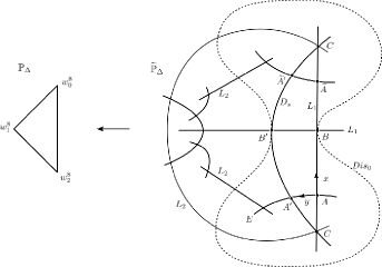
Figure 1. Figure 1. $\mathbb{P}_{\Delta}$ and a resolution $\widetilde{\mathbb{P}}_{\Delta}$. The components $L_{1},L_{2},D_{s}$ and $Dis_{0}$ of the discriminant are also depicted in the right.

4.2. Discriminant loci

Our family over $\mathbb{P}_{\Delta}$ is either $\mathcal{V}_{\mathbb{Z}_{8}}^{1}$ or $\mathcal{V}_{\mathbb{Z}_{8}\times\mathbb{Z}_{8}}^{1}$, whose general fibers are given by $V_{8,w}^{1}/\left\langle\tau\right\rangle$ or $V_{8,w}^{1}/\left\langle\sigma,\tau\right\rangle$, respectively. In either case, since the quotients are taken by free group actions, the degenerations occur at the same loci as the $(2,2,2,2)$ complete intersection $V_{8,w}$ summarized in Proposition 3.5. We have depicted in Fig.1 schematically the components of the proper transforms of the discriminant loci. For simplicity we use the same letters $L_{1},L_{2},D_{s}$ for the proper transforms, but it should be clear in the context. Using the affine coordinate (4.2), they are given by

$$\qquad\qquad\qquad\qquad\quad D_{s}=\left\{1+4x+y=0\right\}$$

$$L_{1}=\left\{w_{1}=0\right\}\cup\left\{4x-1=0\right\},\;\;L_{2}=\left\{w_{0}w_{2}=0\right\}\cup\left\{4x+1\right\}\cup Dis_{0},$$

where the component $Dis_{0}$ is defined by $dis_{0}=0$ with

$$dis_{0}=(1-4x)^{4}-256xy(1+4x+y).$$

The component $Dis_{0}$ will play an important role when describing mirror symmetry at genus one.

4.3. Degeneration points

In the next section, we will study the degenerations of the family over the resolution $\widetilde{\mathbb{P}}_{\Delta}$ in terms of period integrals of the family. In the context of mirror symmetry, we are mostly interested in special boundary points called large complex structure limits (LCSLs) which are characterized by certain distinguished monodromy properties of period integrals (see [Mo] for a precise definition and also Appendix C). It turns out that there are many LCSLs in $\widetilde{\mathbb{P}}_{\Delta}$ where mirror symmetry emerges in nice forms (see Proposition 7.9 for our final interpretations). In Fig.1, we have named them $A,A^{\prime};B,B^{\prime};C$ and also $\tilde{A},\tilde{A}^{\prime}$.

4.3.a. $A$ and $A^{\prime}$. Here and in what follows, we will use the affine coordinate $(x,y)$ introduced in (4.2). This affine coordinate arises as one of the affine coordinate of the blow-up of the $A_{1}$ singularity at the vertex $w_{2}^{8}$ of $\mathbb{P}_{\Delta}$, where three components of the discriminant $L_{1},L_{2}$ and $D_{s}$ intersect. After the blow-up, the intersection splits into three points on the exceptional divisor $E$. Two of them, $A$ and $A^{\prime}$, are LCSLs which were studied locally in [Pav].

4.3.b. Symmetry $w_{0}\leftrightarrow w_{2}$. The points $A,A^{\prime},\tilde{A},\tilde{A}^{\prime},B,B^{\prime}$ and $C$ in Fig.1 all give rise to LCSLs, which we will study in detail in Sections 5, 6 and 7. In terms of the affine coordinate $x,y$ in (4.2), they are given by

$$A=(0,0),A^{\prime}=(0,-1);\,\,B=(\frac{1}{4},0),B^{\prime}=(\frac{1}{4},-2);\,\,C=(-\frac{1}{4},0).$$

The coordinates of $\tilde{A}$ and $\tilde{A}^{\prime}$ are given by $(\frac{1}{16}\frac{1}{x},\frac{1}{4}\frac{y}{x})=(0,0)$ and $(0,-1)$, respectively. In fact, all the boundary divisors are invariant under the following involution:

(4.3) $$(x,y)\mapsto(\frac{1}{16}\frac{1}{x},\frac{1}{4}\frac{y}{x}),$$

which comes from the symmetry of $\widetilde{\mathbb{P}}_{\Delta}$ under the exchange $w_{0}\leftrightarrow w_{2}$. Actually, this symmetry is represented by the action of $\bar{S}^{4}$ in $G_{max}$ described in Proposition 3.10. The points $B,B^{\prime}$ and $C$ are fixed under this involution, while $A$ and $A^{\prime}$ are transformed to $\tilde{A}$ and $\tilde{A}^{\prime}$, respectively. One might consider the quotient $\mathbb{P}_{\Delta}/\left\langle\bar{S}^{4}\right\rangle=\mathbb{P}_{w}^{2}/G_{max}$ as a parameter space of the families, but as we saw in Proposition 3.12, the quotient does not admit the corresponding family over $\mathbb{P}_{\Delta}/\left\langle\bar{S}^{4}\right\rangle$.

5. Mirror symmetry from the boundary points $A$ and $A^{\prime}$

Associated to the family $\mathcal{V}_{\mathbb{Z}_{8}}^{1}\rightarrow\mathbb{P}_{\Delta}$ (resp. $\mathcal{V}_{\mathbb{Z}_{8}\times\mathbb{Z}_{8}}^{1}\rightarrow\mathbb{P}_{\Delta}$) we have the local system $R^{3}\pi_{*}\mathbb{C}_{\mathcal{V}_{\mathbb{Z}_{8}}^{1}}$(resp. $R^{3}\pi_{*}\mathbb{C}_{\mathcal{V}_{\mathbb{Z}_{8}\times\mathbb{Z}_{8}}^{1}}$) over $\mathbb{P}_{\Delta}$. These local systems result in a system of differential equations (Picard-Fuchs equations) of the same forms, which were studied locally in [Pav]. We will study the resulting Picard-Fuchs equations globally, and find in Section 8 that a difference between the two local systems appears in the integral structures for the solutions of the Picard-Fuchs equations (i.e., in the integral variation of Hodge structures). Also, we will recognize the difference between the two families when we calculate genus one Gromov-Witten potentials (see Remark 5.11 and Remark 7.5).

5.1. Picard-Fuchs equations

As discovered first in [CdOGP], we can find mirror symmetry in calculating genus zero Gromov-Witten invariants from the period integrals which we determine by solving Ficard-Fuchs equations.

5.1.a. Period integrals. Since the both families $\mathcal{V}_{\mathbb{Z}_{8}}^{1}$ and $\mathcal{V}_{\mathbb{Z}_{8}\times\mathbb{Z}_{8}}^{1}$ come from the same family $\mathcal{V}^{1}\rightarrow\mathbb{P}_{w}^{2}$ of the Heisenberg-invariant $(2,2,2,2)$ complete intersections in $\mathbb{P}^{7}$, we can express the period integrals following [Gr]:

(5.1) $$\Pi_{\gamma}(w):=\int_{\gamma}Res\left(\frac{w_{2}^{4}}{f_{1}(w,x)f_{2}(w,x)f_{3}(w,x)f_{4}(w,x)}d\mu\right),$$

where $d\mu:={\displaystyle\sum_{i=0}^{7}(-1)^{i}dx_{0}\wedge\cdots\widehat{dx_{i}}\cdots\wedge dx_{7}}$ and $\gamma$ is an integral cycle of a fixed fiber of the family. Period integral in this form often appears when describing mirror symmetry; there, we combine the integral over a cycle with the residue to an integral over a tubular cycle $T(\gamma)$ of the zero locus $f_{1}=\cdots=f_{4}=0$. It is straightforward to evaluate the period integral over a tubular cycle

$$T(\gamma_{0}):=\left\{[x]\in\mathbb{P}^{7}\mid\left|x_{i}/x_{0}\right|=\mathcal{\varepsilon}\,\,(i=1,\cdots,7)\right\}.$$

The following results are obtained in [Pav]:

Proposition 5.1.

$(1)$ The integral $\Pi_{\gamma_{0}}(w)$ can be evaluated in a closed formula.

$(2)$ In the affine coordinate $x,y$ of (4.2), the integral $\Pi_{\gamma_{0}}(w)=:w_{0}(x,y)$ has the following power series expansion,

(5.2) $$\omega_{0}(x,y)=1+8x^{2}+16xy+160x^{2}y+16xy^{2}+88x^{4}+1536x^{3}y+\cdots.$$

Proof.

Since all calculations are now standard in literatures (see e.g. [BaCo]), we only sketch them. We first write quadric equations as

$$\frac{1}{w_{2}}\frac{1}{x_{i+1}x_{i+5}}f_{i}(w,x)=1-P_{i}(w,x)\,\,\,(i=1,...,4)$$

in terms of Laurent polynomials $P_{i}$, and evaluate the residues in the coordinate $x_{0}=1$ by making geometric series,

$$\Pi_{\gamma_{0}}(w)=\int_{T(\gamma_{0})}\sum_{n_{1},...,n_{4}\geq 0}P_{1}(w,x)^{n_{1}}\cdots P_{4}(w,x)^{n_{4}}\frac{dx_{1}\cdots dx_{7}}{x_{1}\cdots x_{7}}.$$

We need to have careful analysis to formulate a closed formula which we refer to [Pav, III.9]. However it is straightforward to have the series expansion up to considerably higher order in $x,y$ (say total degree 50) which is sufficient for our purpose. ∎

From the series expansion (5.2) up to sufficiently high degrees, we can determine Picard-Fuchs differential operators which annihilate the period integral. The following $\mathcal{D}_{2}$ and $\mathcal{D}_{3}$ were first determined in [Pav].

Proposition 5.2.

The period integral (5.2) satisfy the following set of differential equations of Fuchs type:

(5.3) $$\mathcal{D}_{2}w(x,y)=0,\,\,\,\,\,\,\mathcal{D}_{3}w(x,y)=0,$$

where $\mathcal{D}_{2}$ and $\mathcal{D}_{3}$ are the second and third order differential operators, see Appendix A for their explicit forms.

5.1.b. Characteristic variety. It is straightforward to determine the singular loci (characteristic variety) of the above differential operators; we obtain $\left\{dis_{k}=0\right\}$ with

$$dis_{0}:=(1-4x)^{4}-256xy(1+4x+y),$$

$$dis_{1}:=1+4x+y,\,\,\,\,dis_{2}:=1+4x\;\;\;and\;\;\;dis_{3}:=1-4x,$$

in addition to the coordinate lines $\left\{x=0\right\},\left\{y=0\right\}$. We note that each component of the characteristic variety corresponds exactly to one of the degenerations summarized in Subsection 4.2.

5.1.c. Picard-Fuchs equations at $A^{\prime}$. The differential operators $\mathcal{D}_{2}$ and $\mathcal{D}_{3}$ are easily transformed to the affine coordinate $(x_{1},y_{1})$ centered at the boundary point $A^{\prime}$ by the relation

(5.4) $$(x_{1},y_{1})=(x,-4x-y-1).$$

The local geometry around $A$ and $A^{\prime}$ is summarized in Fig.2. We denote by $\mathcal{D}_{2}^{\prime}$ and $\mathcal{D}_{3}^{\prime}$, respectively, the resulting differential operators from $\mathcal{D}_{2}$ and $\mathcal{D}_{3}$.

Proposition 5.3.

The local solutions of $\mathcal{D}_{2}^{\prime}\omega=\mathcal{D}_{3}^{\prime}\omega=0$ around $(x_{1},y_{1})=(0,0)$ have exactly the same forms as those of $\mathcal{D}_{2}\omega=\mathcal{D}_{3}\omega=0$ around $(x,y)=(0,0)$.

Proof.

Let us denote the simple replacements of variables by $\mathcal{D}_{k}(x_{1},y_{1}):=\mathcal{D}_{k}|_{{x\rightarrow x_{1}\atop y\rightarrow y_{1}}}$ for $k=2,3$. Calculating the coordinate transformations $\mathcal{D}_{2}^{\prime},\mathcal{D}_{3}^{\prime}$, we find the following relations

$$\mathcal{D}_{2}(x_{1},y_{1})=y_{1}^{2}\mathcal{D}_{2}^{\prime},\,\,\,\,\mathcal{D}_{3}(x_{1},y_{1})=y_{1}\mathcal{D}_{3}^{\prime}-5(1+4x_{1}+2y_{1})\theta_{y_{1}}\mathcal{D}_{2}^{\prime}-5y_{1}\mathcal{D}_{2}^{\prime}.$$

These relations implies the claimed property. ∎

We remark, for later use, that there is the following invariant relation

$$y(1+4x+y)=y_{1}(1+4x_{1}+y_{1})$$

under the coordinate change $(x_{1},y_{1})=(x,-4x-y-1)$.

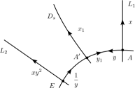
Figure 2. Figure 2. Boundary points $A$ and $A^{\prime}$

5.2. Griffiths-Yukawa couplings

Let us denote by $\Omega(w)$ the holomorphic three form on a general fiber $V_{8,w}^{1}/\mathbb{Z}_{8}$ of the family $\mathcal{V}_{\mathbb{Z}_{8}}^{1}$ over $\mathbb{P}_{\Delta}$, by which we express the period integral (5.1) as $\Pi_{\gamma}(w)=\int_{\gamma}\Omega(w)$.

5.2.a. Near the point $A$. We define the so-called Griffiths-Yukawa couplings by

(5.5) $$C_{ijk}^{A}:=-\int_{V_{8,w}^{1}/\mathbb{Z}_{8}}\Omega(w)\frac{\partial^{3\;}}{\partial z_{A}^{i}\partial z_{A}^{j}\partial z_{A}^{k}}\Omega(w)$$

where $(z_{A}^{1},z_{A}^{2})=(x,y)$ is the affine coordinate centered at the degeneration point $A$. Using the Picard-Fuchs equations (see e.g. [HKTY1]), we have

Proposition 5.4.

Up to a common constant d, the Griffiths-Yukawa couplings $C_{111}^{A},C_{112}^{A},C_{122}^{A}$ and $C_{222}^{A}$ are determined in order as follows:

$$\frac{d\,P_{111}}{x^{3}dis_{0}\,dis_{1}^{2}\,dis_{2}\,dis_{3}},\,\,\,\,\frac{d\,P_{112}}{x^{2}y\,dis_{0}\,dis_{1}^{2}\,dis_{3}},\,\,\,\,\frac{d\,P_{122}}{xy\,dis_{0}\,dis_{1}^{2}\,dis_{3}},\,\,\,\,\frac{d\,P_{222}}{y^{2}dis_{0}\,dis_{1}^{2}},$$

where $P_{ijk}=P_{ijk}(x,y)$ are polynomials given in Appendix B $($see also [HT21]$)$.

In Proposition 5.7, we determine the overall constant $d$ in $C_{ijk}^{A}$ by finding mirror symmetry of the family $\mathcal{V}_{\mathbb{Z}_{8}}^{1}$ to a Calabi-Yau manifold $V_{8,w}^{1}$.

5.2.b. Near the point $A^{\prime}$. In the same way as above, we define the Griffiths-Yukawa couplings $C_{ijk}^{A^{\prime}}$ in terms of the affine coordinate $(z_{A^{\prime}}^{1},z_{A^{\prime}}^{2})=(x_{1},y_{1})$ centered at $A^{\prime}$. As above, they are determined by the Picard-Fuchs equations $\mathcal{D}_{2}^{\prime}\omega=\mathcal{D}_{3}^{\prime}\omega=0$ up to a normalization. However, due to the properties in Proposition 5.3, we see that the isomorphism $C_{ijk}^{A^{\prime}}=C_{ijk}^{A}$, i.e., $C_{ijk}^{A^{\prime}}(x_{1},y_{1})=C_{ijk}^{A}(x_{1},y_{1}).$

5.3. Mirror symmetry

For a boundary point $P=D_{1}\cap D_{2}$ given as a normal crossing divisors, by solving the Picard-Fuchs equations around $P$, we can study the local monodromies around boundary divisors $D_{1},D_{2}$. Mirror symmetry of the family $\mathcal{V}_{\mathbb{Z}_{8}}^{1}$ to a Calabi-Yau manifold $M$ arises at a special boundary point called the large complex structure limit (LCSL), which is characterized by unipotent monodromy properties around the boundary divisors; these special forms of monodromies define the so-called monodromy weight filtration on the third cohomology space $H^{3}(V_{8,w}^{1}/\mathbb{Z}_{8},\mathbb{R})$. As one of the consequences of mirror symmetry, we observe an isomorphism between the weight monodromy filtration and the corresponding filtration in the hard Lefschetz theorem applied for the mirror Calabi-Yau manifold $M$ (see e.g. [HT18, Sect.2]).

Proposition 5.5.

The boundary points $A$ and $A^{\prime}$, respectively, of the Picard-Fuchs equations over $\mathbb{P}_{\Delta}$ are mirror symmetric to Calabi-Yau manifolds $X:=V_{8w}^{1}$ and $X^{\prime}:=V_{8,w}^{2}$ in the above sense.

We can verify the above proposition from the weight monodromy filtrations which we introduce by using the canonical forms (see Appendix C) of local solutions around $A$ and $A^{\prime}$. Here we remark that there is no distinction between $A$ and $A^{\prime}$ as far as local properties are concerned as we observed in Proposition 5.3. Similarly, there is no distinction for the filtrations coming from the hard Lefschetz theorem for $V_{8,w}^{1}$ and its birational model $V_{8,w}^{2}$. In the above proposition, we have fixed one way of the mirror identification and we will retain this in what follows.

5.4. Mirror symmetry and Gromov-Witten invariants

Mirror symmetry observed in Proposition 5.5 can be confirmed by extracting their quantum cohomology from the Griffiths-Yukawa couplings (5.5) expanded near the boundary points. This was first achieved in [Pav], however we reproduce it here in order to fit the results into our global study of the family over $\mathbb{P}_{\Delta}$.

5.4.a. Mirror maps. Near the boundary point $A$, it is straightforward to solve the Picard-Fuchs equations $\mathcal{D}_{2}\omega=\mathcal{D}_{3}\omega=0$ in the forms of power series with logarithmic singularities around the boundary divisors $\left\{x=0\right\}$ and $\left\{y=0\right\}$. The solutions consist of six independent power series, which have the following leading logarithmic singularities:

$$\omega_{0}=1, \omega_{1}=\log x, \omega_{2,1}=(\log x)^{2}+2(\log x)(\log y),$$

$$\omega_{2}=\log y, \omega_{2,2}=(\log x)^{2}, \omega_{3}=(\log x)^{3}+3(\log x)^{2}(\log y).$$

This structure of the logarithmic singularities in the solutions actually defines the weight monodromy filtration $W_{0}\subset W_{2}\subset W_{4}\subset W_{6}$, see Appendix C. For our purpose here, we only need to determine the explicit forms of the solutions $\omega_{0},\omega_{1},\omega_{2}$. Note that the solution $\omega_{0}$ is unique by the leading behavior $\omega_{0}=1$, which is given by (5.2). On the other hand the solutions $\omega_{1},\omega_{2}$ are determined up to adding constant multiples of $\omega_{0}$; we set these solutions as

$$\omega_{1}=\omega_{0}\log x+\omega_{1}^{reg}+c_{1}\omega_{0},\,\,\,\omega_{2}=\omega_{0}\log y+\omega_{2}^{reg}+c_{2}\omega_{0},$$

where $\omega_{k}^{reg}$ represent power series with no constant terms.

Definition 5.6.

We define mirror map by the inverse relations $x=x(q_{1},q_{2}),$ $y=y(q_{1},q_{2})$ of

$$q_{1}=e^{\frac{\omega_{1}}{\omega_{0}}}=C_{1}x\,\exp\big{(}\frac{\omega_{1}^{reg}}{\omega_{0}}\big{)},\,\,\,\,q_{2}=e^{\frac{\omega_{2}}{\omega_{0}}}=C_{2}y\,\exp\big{(}\frac{\omega_{2}^{reg}}{\omega_{0}}\big{)},$$

where $C_{k}:=e^{c_{k}}$. Also we often write $q_{k}=e^{t_{k}}(k=1,2)$ with introducing $t_{k}$.

5.4.b. Griffiths-Yukawa couplings. Mirror symmetry arises from the family $\mathcal{V}_{\mathbb{Z}_{8}}^{1}$ if we combine Griffiths-Yukawa couplings in Proposition 5.4 with the mirror maps near the boundary point [CdOGP]. We recall that the so-called quantum corrected Yukawa couplings are defined by

(5.6) $$Y_{abc}^{A}=\big{(}\frac{1}{\omega_{0}}\big{)}^{2}\sum_{i,j,k}C_{ijk}^{A}\frac{dz_{A}^{i}}{dt_{a}}\frac{dz_{A}^{j}}{dt_{b}}\frac{dz_{A}^{k}}{dt_{c}},$$

where $(z_{A}^{1},z_{A}^{2}$) represents the mirror map $(x,y)=(x(q_{1},q_{2})$, $y(q_{1},q_{2}))$ at the boundary point $A$, and the substitution of the mirror map is assumed in the r.h.s. Similarly we have the quantum corrected Yukawa couplings $Y_{abc}^{A^{\prime}}$ with $C_{ijk}^{A^{\prime}}$ and the mirror map $z_{A^{\prime}}^{i}$ defined around the other boundary point $A^{\prime}$.

Proposition 5.7.

When we set $d=1$ in $C_{ijk}^{A}$ and $C_{1}=C_{2}=1$ in the definition of mirror map, we have

$$Y_{111}^{A}=16+512\,q_{1}q_{2}+22528\,q_{1}^{2}q_{2}\cdots, Y_{112}^{A}=16+512\,q_{1}q_{2}+11264\,q_{1}^{2}q_{2}\cdots,$$

$$Y_{122}^{A}=0+512\,q_{1}q_{2}+5632\,q_{1}^{2}q_{2}\cdots, Y_{222}^{A}=0+64\,q_{2}+512\,q_{1}q_{2}+64\,q_{2}^{2}\cdots.$$

Also, we have exactly same form for the corresponding expansions of $Y_{abc}^{A^{\prime}}$.

Quantum corrected Yukawa couplings are related to the so-called genus zero Gromov-Witten potential $F_{0}^{A}$ , by $Y_{abc}^{A}=\frac{\partial^{3}F_{0}^{A}}{\partial t^{a}\partial t^{b}\partial t^{c}}.$ From this potential function, we read Gromov-Witten invariants and also classical cubic forms (2.6) in the following form:

$$F_{0}^{A}=\frac{16}{3!}\,t_{1}^{3}+\frac{16}{2!}t_{1}^{2}t_{2}+\sum_{d_{1},d_{2}}N_{0}^{A}(d_{1},d_{2})q_{1}^{d_{1}}q_{2}^{d_{2}},$$

where the summation over the bi-degrees $\beta:=(d_{1},d_{2})$ is restricted to $d_{1},d_{2}\geq 0$ and $(d_{1},d_{2})\not=(0,0)$ (see 7.5 of Section 7 for a more invariant form of $F(t)$).

Proposition 5.8.

Assuming mirror symmetry, the numbers $N_{0}^{A}(\beta)$ are Gromov-Witten invariants of stable maps to $V_{8,w}^{1}$ with $\beta\not=0\in H_{2}(V_{8,w}^{1},\mathbb{Z})$. The bi-degree $(d_{1},d_{2})$ represents the degrees $(\beta.H_{X},\beta.A_{X})$ with respect to the divisor classes $H_{X}=H_{1}$ and $A_{X}=A_{1}$ introduced in $($2.6$)$ and 2.2.

Similar results hold for the numbers $N_{0}^{A^{\prime}}(d_{1},d_{2})$ with $V_{8,w}^{1}$ being replaced by the birational model $V_{2,w}^{2}$, and divisors $H_{1},A_{1}$ replaced by $H_{2},\tilde{A}_{2}$ in 2.4.

It is convenient to define BPS numbers $n_{0}(\beta):=n_{0}(d_{1},d_{2})$ by the relations

$$N_{0}^{A}(\beta)=\sum_{k|\beta}\frac{1}{k^{3}}n_{0}^{A}(\beta/k),$$

which remove the contributions from the so-called multiple covers [AM2, Vo] in $N_{0}^{A}(\beta)=N_{0}^{A}(d_{1},d_{2})$. In Table 1 (0), we list the resulting BPS numbers from $F_{0}^{A}$.

Results in this subsection were first obtained in [Pav] verifying that some of BPS numbers coincides with rational curves on $V_{8,w}^{1}$. The identification of the two boundary points $A$ and $A^{\prime}$, respectively, with the birational models $V_{8,w}^{1}$ and $V_{8,w}^{2}$ is justified by observing the number of flopping curves in $n_{0}^{A}(0,1)=n_{0}^{A^{\prime}}(0,1)=64$, and also a “sum-up relation”

(5.7) $$n_{0}^{(2,2,2,2)}(d)=\sum_{d_{2}}n_{0}^{A}(d,d_{2})=\sum_{d_{2}}n_{0}^{A^{\prime}}(d,d_{2}),$$

which reproduce the BPS numbers in Tables E1 (1) of Appendix E for a smoothing of the singular Calabi-Yau variety $X_{2,2,2,2}^{sing}$ arising from the contractions of 64 curves;

(5.8) $$\begin{matrix}\lx@xy@svg{\hbox{\raise 0.0pt\hbox{\kern 54.10669pt\hbox{{\hbox{\kern-54.10669pt\raise 0.0pt\hbox{\hbox{\kern 6.0pt\raise-2.87222pt\hbox{$\textstyle{V^{1}_{8,w}}$}}}}}{\hbox{\kern 31.25113pt\raise 0.0pt\hbox{\hbox{\kern 6.0pt\raise-2.87222pt\hbox{$\textstyle{V^{2}_{8,w}}$}}}}}{\hbox{\kern-26.80121pt\raise-36.98839pt\hbox{\hbox{\kern 6.0pt\raise-2.89333pt\hbox{$\textstyle{\;\;\;\;X_{2,2,2,2}^{sing}\;.}$}}}}}{\hbox{\kern-42.66003pt\raise-19.91682pt\hbox{\hbox{\kern 6.0pt\raise-3.5pt\hbox{$\textstyle{\,{}^{\,{}_{64\,\mathbb{P}^{1}}}}$}}}}}{\hbox{\kern 19.9357pt\raise-19.91682pt\hbox{\hbox{\kern 6.0pt\raise-3.5pt\hbox{$\textstyle{\,{}^{\,{}_{64\,\mathbb{P}^{1}}}}$}}}}}\ignorespaces\ignorespaces\ignorespaces\ignorespaces{\hbox{\kern-31.25113pt\raise 0.0pt\hbox{\hbox{\kern 0.0pt\raise 0.0pt\hbox{\lx@xy@tip{1}\lx@xy@tip{-1}}}}}}\ignorespaces\ignorespaces\ignorespaces{\hbox{\lx@xy@drawline@}}\ignorespaces\ignorespaces{\hbox{\kern-3.0pt\raise 0.0pt\hbox{{}\hbox{\kern 0.0pt\raise 0.0pt\hbox{\hbox{\kern 3.0pt\hbox{\hbox{\kern 0.0pt\raise 0.0pt\hbox{$\scriptstyle{}$}}}\kern 3.0pt}}}}}}\ignorespaces{\hbox{\kern 31.25113pt\raise 0.0pt\hbox{\hbox{\kern 0.0pt\raise 0.0pt\hbox{\lx@xy@tip{1}\lx@xy@tip{-1}}}}}}\ignorespaces\ignorespaces\ignorespaces{\hbox{\lx@xy@drawline@}}\ignorespaces{\hbox{\lx@xy@drawline@}}\ignorespaces\ignorespaces\ignorespaces\ignorespaces\ignorespaces{}\ignorespaces\ignorespaces\ignorespaces{\hbox{\lx@xy@drawline@}}\ignorespaces{\hbox{\kern-13.59378pt\raise-25.20174pt\hbox{\hbox{\kern 0.0pt\raise 0.0pt\hbox{\lx@xy@tip{1}\lx@xy@tip{-1}}}}}}\ignorespaces\ignorespaces\ignorespaces{\hbox{\lx@xy@drawline@}}\ignorespaces{\hbox{\lx@xy@drawline@}}\ignorespaces\ignorespaces\ignorespaces\ignorespaces\ignorespaces{}\ignorespaces\ignorespaces\ignorespaces{\hbox{\lx@xy@drawline@}}\ignorespaces{\hbox{\kern 13.60529pt\raise-25.20174pt\hbox{\hbox{\kern 0.0pt\raise 0.0pt\hbox{\lx@xy@tip{1}\lx@xy@tip{-1}}}}}}\ignorespaces\ignorespaces\ignorespaces{\hbox{\lx@xy@drawline@}}\ignorespaces{\hbox{\lx@xy@drawline@}}\ignorespaces}}}}\end{matrix} \textstyle{V^{1}_{8,w}} \textstyle{V^{2}_{8,w}} \textstyle{\;\;\;\;X_{2,2,2,2}^{sing}\;.} \textstyle{\,{}^{\,{}_{64\,\mathbb{P}^{1}}}} \textstyle{\,{}^{\,{}_{64\,\mathbb{P}^{1}}}} \textstyle{V^{1}_{8,w}} \textstyle{V^{2}_{8,w}} \textstyle{\;\;\;\;X_{2,2,2,2}^{sing}\;.} \textstyle{\,{}^{\,{}_{64\,\mathbb{P}^{1}}}} \textstyle{\,{}^{\,{}_{64\,\mathbb{P}^{1}}}}$$

5.5. Counting functions by quasi-modular forms

Actually, mirror symmetry of Calabi-Yau manifolds which have abelian surface fibration was first studied in the case of fiber product of two rational elliptic surfaces, i.e., Schoen’s Calabi-Yau threefolds [HSS, HST1]; there it was found that some part of Gromov-Witten potential are expressed by quasi-modular forms coming from elliptic curves. It is interesting to observe that the Gromov-Witten potential of $V_{8,w}^{1}$ has similar properties.

Let us define $q$-series $Z_{0,n}(q)\,(n=1,2,...)$ by

(5.9) $$F_{0}^{A}(q,p)=\frac{16}{3!}\,t_{1}^{3}+\frac{16}{2!}t_{1}^{2}t_{2}+\sum_{n\geq 1}Z_{0,n}(q)p^{n},$$

where $F_{0}^{A}(q,p)=F_{0}^{A}(q_{1},q_{2})$. By definition of the bi-degree $(d_{1},d_{2})$, the $q$-series $Z_{0,n}^{A}(q)=\sum_{d\geq 0}N_{0}^{A}(d,n)q^{d}$ counts the Gromov-Witten invariants related to curves which intersects with the fiber class $n$-times, i.e., $n$-sections of the fibration $V_{8,w}^{1}\rightarrow\mathbb{P}^{1}$. In particular, since it holds that

$$Z_{0,1}^{A}(q)=\sum_{d\geq 0}N_{0}^{A}(d,1)q^{d}=\sum_{d\geq 0}n_{0}^{A}(d,1)\,q^{d},$$

the $q$-series $Z_{0,1}(q)$ counts BPS numbers of the sections. We can observe the following property from the table of BPS numbers:

Observation 5.9.   The $q$-series $Z_{0,1}(q)$ has a closed form given by

$$Z_{0,1}^{A}(q)=\frac{64}{\bar{\eta}(q)^{8}},$$

where $\bar{\eta}(q)=\Pi_{n\geq 1}(1-q^{n})$. Moreover, we have

$$Z_{0,n}^{A}(q)=P_{0,n}^{A}(E_{2},E_{4},E_{6})\left(\frac{64}{\bar{\eta}(q)^{8}}\right)^{n},$$

where $P_{0,n}^{A}(E_{2},E_{4},E_{6})$ are quasi-modular forms of weight $4(n-1)$ in terms of Eisenstein series $E_{2},E_{4}$ and $E_{6}$.

We have verified the above properties by calculating $Z_{0,n}(q)$ up to sufficiently large degree $d\leq 70$ and for $n\leq 9$. Below are explicit forms of the resulting polynomials $P_{0,n}^{A}$ for lower $n$;

$$P_{0,2}^{A}= \frac{1}{4608}(8\,E_{2}^{2}+E_{4}),$$

$$P_{0,3}^{A}= \frac{1}{2654208}(14E{}_{2}^{4}+7E{}_{2}^{2}E_{4}+E{}_{4}^{2}+2E_{2}E_{6}),$$

$$P_{0,4}^{A}= \frac{1}{2^{26}3^{7}}(3008E{}_{2}^{6}+2808E{}_{2}^{4}E_{4}+1128E{}_{2}^{2}E{}_{4}^{2}+125E{}_{4}^{3}$$

$${\hskip 90.0pt}+1120E{}_{2}^{3}E_{6}+528E_{2}E_{4}E_{6}+31E_{6}^{2}).$$

The forms of $P_{0,n}^{A}\,(5\leq n\leq 9)$ can be found in [HT21].

5.6. Counting sections by geometry of singular fibers

It is easy to identify the number $64$ with the number of the sections of $X=V_{8,w}^{1}\rightarrow\mathbb{P}^{1}$. The appearance of the $\eta$-function in the denominator reminds us of similar counting formulas for a rational elliptic surface in Schoen’s Calabi-Yau manifolds [HSS, HST1], which came from 12 singular fibers of Kodaira’s $I_{1}$ type. In the present case, the singular fibers consist of 8 elliptic translation scrolls,

$$S_{k}=\bigcup_{p\in E_{k}}\langle p,p+e_{k}\rangle\,\,\,\,\,(k=1,...,8)$$

which is described in the part 2.2 (2), where $\langle p,p+e_{k}\rangle$ represents a line passing two points $p$ and $p+e_{k}$$(e_{k}\in E_{k})$. Clearly, the power 8 in the denominator of $Z_{0,1}^{A}(a)=\frac{64}{\bar{\eta}(q)^{8}}$ should be explained by the number of singular fibers. Since $N_{0}^{A}(\beta)=n_{0}^{A}(\beta)$ holds for the classes $\beta=(\beta\cdot H_{X},\beta\cdot A_{X})=(d,1)$, the function $\frac{64}{\bar{\eta}(q)^{8}}$ should count the numbers of rational curves coming from the 8 translation scrolls. Let us fix a section $\sigma$ and denote chains of lines contained in translation scrolls $S_{k}\,(k=1,...,8)$ by

$$L_{1}^{(1)},....,L_{n_{1}}^{(1)};L_{1}^{(2)},....,L_{n_{2}}^{(2)};\cdots;L_{1}^{(8)},....,L_{n_{8}}^{(8)},$$

where $\sigma$ intersect at one point with some line $L_{n_{i}}^{(k)}$ in the chain $L_{1}^{(k)},...,L_{n_{k}}^{(k)}$. These chains of rational curves could explain the counting function $\frac{1}{\bar{\eta}(q)^{8}}$, if a configuration

$$\sigma_{X}\cup L_{1}^{(k)}\cup L_{2}^{(k)}\cup\cdots\cup L_{n_{k}}^{(k)}\,\text{with a fixed }k$$

had a contribution $p(n_{k})(:=$the number of partitions of $n_{k}$) to $n_{0}(d,1)=n_{0}(n_{1}+n_{2}+\cdots+n_{8},1)$. However, as one easily recognize, a naive counting from this configuration is $n_{k}$ instead of $p(n_{k})$, while $p(n_{k})=n_{k}$ holds for $n_{k}\leq 3$. In fact, in [Pav], $n_{0}(d,1)$ for $d=n_{1}+\cdots+n_{8}\leq 3$, i.e., the numbers $n_{0}(1,1)=8\times 64,\,n_{0}(2,1)=44\times 64,\,n_{0}(3,1)=192\times 64$ are explained by studying Gromov-Witten theory for the above configurations. However, for $d>3$, there are missing configurations or contributions to explain $n_{0}(\beta)=n_{0}(d,1)$. We hope that we will come to this problem in a future work.

$$\begin{array}[]{c}{}\begin{array}[]{|c|ccccccccc}\hline\cr{}j\diagdown i{}&0&1&2&3&4&5&6&7&8\\ \hline\cr 0&0&0&0&0&0&0&0&0&0\\ 1&64&512&2816&12288&46464&157696&493056&1441792&3989568\\ 2&0&0&4096&98304&1220608&10813440&76775424&464322560&2480783360\\ 3&0&0&2816&195072&6301056&124829696&1772620032&19764707328&183168532288\\ 4&0&0&0&98304&10567680&478740480&13238665216&261369036800&4018366742528\\ 5&0&0&0&12288&6301056&728901120&40797528064&1437499588608&36413468765248\\ 6&0&0&0&0&1220608&478740480&58763759616&3812602150912&160955539341312\\ :&:&:&:&:&:&:&:&:&:\end{array}\end{array}$$

(0) Genus zero BPS numbers $n_{0}^{A}(i,j)$

$$\begin{array}[]{c}{}\begin{array}[]{|c|cccccccccc}\hline\cr{}j\diagdown i{}&0&1&2&3&4&5&6&7&8&9\\ \hline\cr 0&0&0&0&0&0&0&0&0&8&0\\ 1&0&0&0&0&896&8192&50688&245760&1024768&3807232\\ 2&0&0&0&0&2240&163840&3262464&39583744&358221888&2646376448\\ 3&0&0&0&0&1920&966656&47699968&1190572032&19998058112&255958884352\\ 4&0&0&0&0&4640&2097152&248373248&12249595904&363641449120&7661339901952\\ 5&0&0&0&0&1920&2311168&619652096&57765986304&2933367424384&98849134485504\\ 6&0&0&0&0&2240&2097152&833927680&141594460160&12170949409472&649231850569728\\ 7&0&0&0&0&896&966656&619652096&190239614976&27968653028864&2375812698800128\\ :&:&:&:&:&:&:&:&:&:&:\end{array}\end{array}$$

(1) Genus one BPS numbers $n_{1}^{A}(i,j)$

$$\begin{array}[]{|c|ccccccccccc}\hline\cr{}j\diagdown i{}&0&1&2&3&4&5&6&7&8&9&10\\ \hline\cr 0&0&0&0&0&0&0&0&0&0&0&0\\ 1&0&0&0&0&0&0&256&4096&37568&247808&1332480\\ 2&0&0&0&0&0&0&12288&524288&10758016&145555456&1490690048\\ 3&0&0&0&0&0&0&69120&10266624&465354496&11849469952&209498467584\\ 4&0&0&0&0&0&0&147456&75792384&6951182592&311243702272&8956370026496\\ 5&0&0&0&0&0&0&302592&264691712&47403040000&3616972675072&164270290355456\\ 6&0&0&0&0&0&0&364544&531759104&171942100864&21836284264448&1539526624321536\\ 7&0&0&0&0&0&0&302592&674427904&359333519296&74782408261632&8139227500850176\\ :&:&:&:&:&:&:&:&:&:&:&:\end{array}$$

(2) Genus two BPS numbers $n_{2}^{A}(i,j)$

Table 1. Table 1. BPS numbers $n_{g}^{A}(i,j)$ of $X=V_{8,w}^{1}$ for $g=0,1,2$. These are equal to $n_{g}^{A^{\prime}}(i,j)$ of $V_{8,w}^{2}$.

5.7. Genus one Gromov-Witten potentials $F_{1}^{A}$ and $F_{1}^{A^{\prime}}$

Using mirror symmetry, we can extend Observation 5.5 to genus one Gromov-Witten potentials $F_{1}^{A}$ and $F_{1}^{A^{\prime}}$. Here we start with recalling the general form of the genus one Gromov-Witten potential of a Calabi-Yau threefold $M$ proposed in [BCOV1].

5.7.a. Genus one potential $F_{1}$. Suppose $M$ is a Calabi-Yau threefold with rank$(Pic(M))=2$, and that we have a family of mirror Calabi-Yau manifolds over some parameter space with a boundary point (LCSL) at the origin of an affine coordinate $(x_{1},x_{2})$. Then using mirror map defined near the origin, we have the genus one potential function $F_{1}^{M}$ of $M$ in the following form:

(5.10) $$F_{1}^{M}=\frac{1}{2}\log\Big{\{}\big{(}\frac{1}{\omega_{0}}\big{)}^{3+h^{1,1}-\frac{\chi(M)}{12}}\frac{\partial(x_{1},x_{2})}{\partial(t_{1},t_{2})}dis_{0}^{r_{0}}\prod_{k\geq 1}dis_{k}^{r_{k}}\times\prod_{i}x_{i}^{-1-\frac{c_{2}.H_{i}}{12}}\Big{\}},$$

where $\chi(M)$ is the Euler number of $M$ and $h^{1,1}=h^{1,1}(M)$, and also $c_{2}.H_{i}$ are the linear forms described in 2.4. The notation $dis_{k}$ represents the components of the discriminant of the family over the parameter space. Among them, $dis_{0}$ is reserved to represent the component where the most general degenerations of the fibers appear. The powers $r_{k}$ are unknown parameters which we need to determine from some additional data.

In the present case of $V_{8,w}^{1}$, we use the topological invariants $\chi(V_{8,w}^{1})=0,c_{2}.H_{1}=64$ and $c_{2}.A_{1}=0$ (and the same numbers of the corresponding invariants for $V_{8,w}^{2})$. The unknown parameters $r_{k}$ can be fixed by knowing some of vanishing results on Gromov-Witten invariants.

Proposition 5.10.

Near the boundary point $A$, assuming mirror symmetry, we have the potential function

$$F_{1}^{A}(q,p)=\frac{1}{2}\log\Big{\{}\big{(}\frac{1}{\omega_{0}}\big{)}^{3+2}\frac{\partial(x,y)}{\partial(t_{1},t_{2})}dis_{0}^{-\frac{1}{6}}\,dis_{1}^{-1}\,dis_{2}^{-\frac{2}{3}}\,dis_{3}^{-1}\times x^{-1-\frac{64}{12}}y^{-1}\Big{\}}$$

which gives genus one Gromov-Witten potential of $V_{8,w}^{1}$. For the other boundary point $A^{\prime}$, we have isomorphic form $F_{1}^{A^{\prime}}$ with the same parameters $r_{0}$ and $r_{k}$.

Remark 5.11.

From the above expression of $F_{1}^{A}$, we can convince ourselves that we are working on the family $\mathcal{V}_{\mathbb{Z}_{8}}^{1}\rightarrow\mathbb{P}_{\Delta}$ to describe mirror symmetry. This comes from the well-known observation (see e.g. [AM1]) that the power of $dis_{0}^{-\frac{1}{6}}$ is determined by

(5.11) $$-\frac{1}{6}\times(\text{the number of ODPs}),$$

where we count the number of OPDs which appear generically on fiber Calabi-Yau manifolds over the principal component $\left\{dis_{0}=0\right\}$ of the discriminant. The number (5.11) is often called a conifold factor. Recall that we showed in Proposition 3.6 that over $\left\{dis_{0}=0\right\}$ there appear 8 ODPs in $V_{8,w}^{1}$ which lies on a single $\tau$-orbit. Namely, there appears $1$ ODP for the free quotient $V_{8,w}^{1}/\mathbb{Z}_{8}$ with $\mathbb{Z}_{8}=\langle\tau\rangle$. $\hfill\square$

We read genus one Gromov-Witten invariants from the following expansion of $F_{1}^{A}$ with $d_{1},d_{2}\geq 0$ and $(d_{1},d_{2})\not=(0,0)$:

(5.12) $$F_{1}^{A}(q,p)=-\frac{c_{2}.H_{X}}{24}\log q-\frac{c_{2}.A_{X}}{24}\log p+\sum_{d_{1},d_{2}}N_{1}^{A}(d_{1},d_{2})q^{d_{1}}p^{d_{2}}.$$

The BPS numbers $n_{1}^{A}(\beta):=n_{1}^{A}(i,j)$ may be introduced through the following relations to genus one Gromov-Witten invariants $N_{1}^{A}(\beta):=N_{1}^{A}(d_{1},d_{2})$:

$$N_{1}^{A}(\beta)=\sum_{k|\beta}\frac{1}{k}\left\{n_{1}^{A}(\beta/k)+\frac{1}{12}n_{0}^{A}(\beta/k)\right\}.$$

BPS numbers are conjectured to be integer invariants coming from certain counting problems of curves in $X=V_{8,w}^{1}$ with homology class $\beta$ [GV, HST2]. For example, $n_{1}^{A}(8,0)$ counts the numbers of elliptic curves in the eight singular fibers of $V_{8,w}^{1}$. To determine the parameters in the above proposition, we have required vanishings $n_{1}^{A}(i,j)=0$ for $i=0,..,3.$ In Table 1 (1), we list the resulting BPS numbers form $F_{1}^{A}(q,p)$.

5.7.b. $q$-series $Z_{1,1}(q)$ via quasi-modular forms. We define genus one $q$-series $Z_{1,n}(q)$ by arranging the expansion (5.12) into

$$F_{1}^{A}=-\frac{c_{2}.H_{X}}{24}\log q+Z_{1,0}(q)+\sum_{n\geq 1}Z_{1,n}^{A}(q)\,p^{n}.$$

The $q$-series $Z_{1,n}^{A}(q)$ is a generating series of genus one Gromov-Witten invariants $N_{1}^{A}(d,n)$. For $n=0$, we observe that non-vanishing invariants appear only at

$$N_{1}^{A}(8d,0)=\sum_{k|d}\frac{1}{k}n_{1}^{A}(8d/k,0)$$

$(d=1,2,...)$ which comes from elliptic curves in singular fibers of abelian fibration $V_{8,w}^{1}\to\mathbb{P}^{1}$ (see 2.2). Including the first term $-\frac{c_{2}.H_{X}}{24}\log q=-\frac{8}{3}\log q$ in the definition $\widehat{Z}_{1,0}(q)=-\frac{c_{2}.H_{X}}{24}\log q+$$Z_{1,0}^{A}(q)$, we have the $q$-series

$$\widehat{Z}_{1,0}(q)=-\frac{c_{2}.H_{X}}{24}\log q-8\,\log\,\bar{\eta}(q^{8})=-8\log\,\eta(q^{8})$$

in terms of Dedekind’s $\eta$-function $\eta(q)=q^{\frac{1}{24}}\Pi_{n\geq 1}(1-q^{n})$. Corresponding to Observation 5.5, we verify the following property up to sufficiently high degrees of $q$.

Observation 5.12.  The q-series $Z_{1,1}^{A}(q)$ is expressed by quasi-modular forms as

$$Z_{1,1}^{A}(q)=P_{1,1}^{A}(q)\,\frac{64}{\bar{\eta}(q)^{8}}$$

where $P_{1,1}^{A}(q)$ is a polynomial

$$P_{1,1}^{A}=\frac{1}{288}\left\{E_{2}^{2}+E_{2}(S+2T+4U)+4(S+2T-5U)^{2}\right\},$$

of Eisenstein series $E_{2}=E_{2}(q)$ and elliptic theta functions

$$S=\theta_{3}(q)^{4},\quad T=\theta_{3}(q^{2})^{4},\quad U=\theta_{3}(q)^{2}\theta_{3}(q^{2})^{2}$$

with $\theta_{3}(q):=\Sigma_{n\in\mathbb{Z}}q^{n^{2}}$.

We have verified similar polynomial expressions of $P_{1,n}^{A}$ for $n<4$ (see Appendix F and [HT21]). We conjecture the following form of $q$-series $Z_{g,n}^{A}(q)$ in terms of quasi-modular forms in general.

Conjecture 5.13.

The $q$-series $Z_{g,n}^{A}(q)\,(n\geq 1)$ is expressed by

$$Z_{g,n}^{A}(q)=P_{g,n}^{A}(E_{2},S,T,U)\left(\frac{64}{\bar{\eta}(q)^{8}}\right)^{n},$$

where $P_{g,n}^{A}$ is polynomial of degree $2(g+n-1)$ of $E_{2},S,T,U$.

In Subsection 6.3, by using mirror symmetry, we will verify the above conjecture for $g=2$ and lower $n$. Here, we remark that we have the same results for $A^{\prime}$ because of the isomorphisms in Proposition 5.3 between $A$ and $A^{\prime}$.

5.7.c. Contraction to $(2,2,2,2)\subset\mathbb{P}^{7}$. We observed in (5.7) that BPS numbers of a smoothing of the singular Calabi-Yau variety $X_{2,2,2,2}^{sing}$ arises from a “sum-up relation”. This relation holds also at genus one;

(5.13) $$n_{1}^{(2,2,2,2)}(d)=\sum_{d_{2}}n_{1}^{A}(d,d_{2})=\sum_{d_{2}}n_{1}^{A^{\prime}}(d,d_{2}),$$

where $n_{1}^{(2,2,2,2)}(d)$ can be found in [HKTY2] (see also Appendix E).

6. Exploring the parameter space $\mathbb{P}_{\Delta}$ globally

In this section and the subsequent section, we shall study the boundary points $B,B^{\prime}$ and also $C$ (and $C^{\prime}$) described in Section 4. We will find that all aspect of mirror symmetry of $V_{8,w}^{k}\,(k=1,2)$ and their free quotients are encoded in a single system of Picard-Fuchs equations (5.3). The entire picture of mirror symmetry will be summarized in Proposition 7.9. As in the preceding section, for brevity, we will retain the notation $\mathbb{P}_{\Delta}$ even if we will make suitable resolutions.

6.1. Blowing-up at the boundary points $B$, $B^{\prime}$

The points $B$ and $B^{\prime}$ are symmetric under the involution (5.4), and there is no difference in the local analysis around $B$ and $B^{\prime}$. Because of this we will restrict our attentions mostly to $B$.

As is clear in the form of the discriminant $dis_{0}$, the two divisors $\left\{dis_{0}=0\right\}$ and $\left\{y=0\right\}$ intersect at $B$ with 4th-order tangency. To have power series solutions of the Picard-Fuchs equation, we blow-up at this point successively four times; and find that the point $\tilde{B}$ shown in Figure 3 has properties of a LCSL. In a similar way, we verify that $\tilde{B}^{\prime}$ is also a LCSL. In what follows, we will use $B$ and $B^{\prime}$ instead of $\tilde{B}$ and $\tilde{B}^{\prime}$ for brevity of notation.

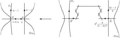
Figure 3. Fig.3. Blowing-up at $B$ and $B^{\prime}$. For brevity of notation, $\widetilde{B}$ and $\widetilde{B}^{\prime}$ are called $B$ and $B^{\prime}$ again in the text.

6.1.a. Picard-Fuchs equations and mirror symmetry. Let us introduce $(z_{B}^{1},z_{B}^{2})$ for the blow-up coordinate centered at $B$. It is related to the affine coordinate $(x^{1},x^{2})=(x,y)$ centered at $A$ by

(6.1) $$(z_{B}^{1},z_{B}^{2})=\big{(}\frac{1}{8}(1-4x),\,\,2^{7}\frac{y}{(1-4x)^{4}}\big{)}.$$

It is straightforward to transform the Picard-Fuchs equations $\mathcal{D}_{2}\omega=\mathcal{D}_{3}\omega=0$ to this coordinate. The normalization factors in this coordinate are chosen so that we have a natural coordinate to describe mirror symmetry, e.g. the integral power series $\omega_{0}^{B}$ in (6.3) below.

Proposition 6.1.

The boundary points $B$ and $B^{\prime}$ of the Picard-Fuchs equations over $\mathbb{P}_{\Delta}$ are mirror symmetric to Calabi-Yau manifolds $Y:=V_{8w}^{1}/\mathbb{Z}_{8}\times\mathbb{Z}_{8}$ and $Y^{\prime}:=V_{8w}^{2}/\mathbb{Z}_{8}\times\mathbb{Z}_{8}$, respectively.

We verify the above proposition by making local solutions of the Picard-Fuchs equations around $B$ and $B^{\prime}$. We can also confirm this by calculating Gromov-Witten invariants from $B$ and $B^{\prime}$.

6.1.b. Griffiths-Yukawa couplings. In the same way as Proposition 5.4, we can determine the Griffiths-Yukawa couplings $C_{ijk}^{B}$ up to a normalization constant. Our global description of the family, however, enables us to determine them uniquely by

(6.2) $$C_{ijk}^{B}:=\sum_{l.m.n}C_{lmn}^{A}\frac{\partial x_{l}}{\partial z_{i}^{B}}\frac{\partial x_{m}}{\partial z_{j}^{B}}\frac{\partial x_{n}}{\partial z_{k}^{B}}.$$

We arrange the local solutions around the point $B$ into the canonical form $\Pi_{B}(z)$ in (C.2). Among the solutions, the first half of $\Pi_{B}(z)$ is sufficient to define the mirror map. These solutions have the following explicit forms:

(6.3) $$\omega_{0}^{B}(z)=1+8z_{1}+56z_{1}^{2}+384z_{1}^{3}+\cdots-8z_{1}^{4}z_{2}-96z_{1}^{5}z_{2}-\cdots,$$

$$\omega_{1}^{B}(z)=(\log z_{1})\omega_{0}^{B}(z)+(4z_{1}+44z_{1}^{2}+\frac{1120}{3}z_{1}^{3}+\cdots-2z_{1}^{4}z_{2}-\cdots),$$

$$\omega_{2}^{B}(z)=(\log z_{2})\omega_{0}^{B}(z)+(-12z_{1}-136z_{1}^{2}-\cdots+96z_{1}^{5}z_{2}+\cdots).$$

Here and hereafter, we omit the superscript $B$ in $z_{i}$ for brevity, unless confusions arise. Mirror map is defined in the same way as Definition 5.6 by inverting the relations

$$q_{1}=e^{\frac{\omega_{1}}{\omega_{0}}}=C_{1}z_{1}\,\exp\big{(}\frac{\omega_{1}^{reg}}{\omega_{0}}\big{)},\,\,\,\,q_{2}=e^{\frac{\omega_{2}}{\omega_{0}}}=C_{2}z_{2}\,\exp\big{(}\frac{\omega_{2}^{reg}}{\omega_{0}}\big{)},$$

where $\omega_{0}=\omega_{0}^{B}$ and $\omega_{i}=\omega_{i}^{B}$ with some constant $C_{k}$. We write the mirror map by $z_{a}=z_{a}(q_{1},q_{2})$ for $a=1,2$. Then the quantum corrected Yukawa couplings are given by

(6.4) $$Y_{ijk}^{B}=\left(\frac{1}{N_{B}\omega_{0}^{B}}\right)^{2}\sum_{a,b,c}C_{abc}^{B}\frac{dz_{a}}{dt_{i}}\frac{dz_{b}}{dt_{j}}\frac{dz_{c}}{dt_{k}},$$

where $N_{B}$ is a constant which we will identify in Proposition 8.1 with the normalization constant of the local solutions in $\Pi_{B}(z)$.

Proposition 6.2.

When we set $N_{B}=\frac{1}{2}$, and $C_{1}=C_{2}=1$ in the definition of the mirror map, we have

$$Y_{111}^{B}=128+4096q_{1}^{8}+180224q_{1}^{16}q_{2}+\cdots, Y_{112}^{B}=16+512q_{1}^{8}q_{2}+11264q_{1}^{16}q_{2}+\cdots,$$

$$Y_{122}^{B}=64q_{1}^{8}q_{2}+704q_{1}^{16}q_{2}+4160q_{1}^{16}q_{2}^{2}+\cdots, Y_{222}^{B}=q_{2}+q_{2}^{2}+q_{3}^{3}+\cdots+8q_{1}^{8}q_{2}+.$$

We have exactly same form for the corresponding expansions of $Y_{ijk}^{B^{\prime}}$.

$$\begin{array}[]{|c|ccccccccccccccc}\hline\cr{}j\diagdown i{}&0&..&8&..&16&..&24&..&32&..&40&..&48&..&56\\ \hline\cr 0&0&..&0&..&0&..&0&..&0&..&0&..&0&..&0\\ 1&1&..&8&..&44&..&192&..&726&..&2464&..&7704&..&22528\\ 2&0&..&0&..&64&..&1536&..&19072&..&168960&..&1199616&..&7255040\\ 3&0&..&0&..&44&..&3048&..&98454&..&1950464&..&27697188&..&308823552\\ 4&0&..&0&..&0&..&1536&..&165120&..&7480320&..&206854144&..&4083891200\\ 5&0&..&0&..&0&..&192&..&98454&..&11389080&..&637461376&..&22460931072\\ 6&0&..&0&..&0&..&0&..&19072&..&7480320&..&918183744&..&59571908608\\ 7&0&..&0&..&0&..&0&..&726&..&1950464&..&637461376&..&81827379400\\ :&:&..&:&..&:&..&:&..&:&..&:&..&:&..&:\end{array}$$

(0) Genus zero BPS numbers $n_{0}^{B}(i,j)$.

$${}\begin{array}[]{|c|cccccccccccccccccccc}\hline\cr{}j\diagdown i{}&0&{}1&{}2&{}3&{}4&{}5&{}6&{}7&{}8&{}9&{}10&{}11&{}12&{}13&{}14&{}15&{}16&{}17&{}18&{}19\\ \hline\cr 0&0&{}8&{}8&{}8&{}8&{}8&{}8&{}8&{}8&{}8&{}8&{}8&{}8&{}8&{}8&{}8&{}8&{}8&{}8&{}8\\ 1&0&{}0&{}0&{}0&{}14&{}16&{}48&{}64&{}152&{}128&{}288&{}256&{}728&{}592&{}1248&{}1216&{}2748&{}2112&{}4224&{}3584\\ 2&0&{}0&{}0&{}0&{}0&{}0&{}0&{}0&{}8&{}24&{}112&{}224&{}704&{}848&{}2368&{}2752&{}7872&{}7944&{}19520&{}21472\\ 3&0&{}0&{}0&{}0&{}0&{}0&{}0&{}0&{}0&{}0&{}0&{}0&{}14&{}48&{}288&{}656&{}2748&{}3648&{}12528&{}17408\\ 4&0&{}0&{}0&{}0&{}0&{}0&{}0&{}0&{}0&{}0&{}0&{}0&{}0&{}0&{}0&{}0&{}8&{}72&{}600&{}1728\\ 5&0&{}0&{}0&{}0&{}0&{}0&{}0&{}0&{}0&{}0&{}0&{}0&{}0&{}0&{}0&{}0&{}0&{}0&{}0&{}0\\ 6&0&{}0&{}0&{}0&{}0&{}0&{}0&{}0&{}0&{}0&{}0&{}0&{}0&{}0&{}0&{}0&{}0&{}0&{}0&{}0\end{array}$$

(1) Genus one BPS numbers $n_{1}^{B}(i,j)$.

$$\begin{array}[]{|c|ccccccccccccccccc}\hline\cr{}j\diagdown i{}&0&{}1&{}..&{}5&{}6&{}7&{}8&{}9&{}10&{}11&{}12&{}13&{}14&{}15&{}16&{}17&{}18\\ \hline\cr 0&0&{}0&{}..&{}0&{}0&{}0&{}0&{}0&{}0&{}0&{}0&{}0&{}0&{}0&{}0&{}0&{}0\\ 1&0&{}0&{}..&{}0&{}4&{}32&{}155&{}456&{}1304&{}2784&{}6336&{}11120&{}22440&{}35360&{}66056&{}97752&{}172768\\ 2&0&{}0&{}..&{}0&{}0&{}0&{}0&{}128&{}696&{}2304&{}7416&{}18704&{}51168&{}110400&{}265376&{}504976&{}1115408\\ 3&0&{}0&{}..&{}0&{}0&{}0&{}0&{}0&{}0&{}0&{}0&{}768&{}5112&{}19872&{}74760&{}211208&{}645364\\ 4&0&{}0&{}..&{}0&{}0&{}0&{}0&{}0&{}0&{}0&{}0&{}0&{}0&{}0&{}0&{}2944&{}23552\\ 5&0&{}0&{}..&{}0&{}0&{}0&{}0&{}0&{}0&{}0&{}0&{}0&{}0&{}0&{}0&{}0&{}0\\ :&:&:&:&:&:&:&:&:&:&:&:&:&:&:&:&:&:\end{array}$$

(2) Genus two BPS numbers $n_{2}^{B}(i,j)$.

Table 2. Table 2. BPS numbers $n_{g}^{B}(i,j)$ of $Y=V_{8,w}^{1}/\mathbb{Z}_{8}\times\mathbb{Z}_{8}$. The blanks “$..$” represent vanishing invariants. These are equal to $n_{g}^{B^{\prime}}(i,j)$ of $V_{8,w}^{2}/\mathbb{Z}_{8}\times\mathbb{Z}_{8}$.

6.2. Genus one Gromov-Witten potentials $F_{1}^{B}$ and $F_{1}^{B^{\prime}}$

We determine the genus one Gromov-Witten potentials $F_{1}^{B}$ and $F_{1}^{B^{\prime}}$ using the general form $F_{1}^{M}$ given in (5.10). Since $B$ and $B^{\prime}$ are isomorphic locally, we only describe $F_{1}^{B}$.

6.2.a. Calculating $F_{1}^{B}$. To apply the general formula (5.10), we introduce the following definitions:

$$disB_{0}=1-(1-4z_{1})(1-8z_{1})z_{2}-16z_{1}^{4}(1-8z_{1})z_{2}^{2}$$

$$disB_{1}=1-4z_{1}+16z_{1}^{4}z_{2},\,\,\,disB_{2}=1-4z_{1},\,\,\,disB_{3}=1-8z_{1}.$$

As in Subsection 5.7, knowing that $B$ corresponds to the free quotient $V_{8,w}^{1}/\mathbb{Z}_{8}\times\mathbb{Z}_{8}$, we can determine the parameters $r_{0}$ and $r_{k}$ in the BCOV formula.

Proposition 6.3.

Near the boundary point $B$, the BCOV potential function has the following form

$$F_{1}^{B}(q)=\frac{1}{2}\log\Big{\{}\big{(}\frac{1}{N_{B}\omega_{0}^{B}}\big{)}^{5}\frac{\partial(z_{1},z_{2})}{\partial(t_{1},t_{2})}disB_{0}^{-\frac{1}{6}}\,disB_{1}^{-1}\,disB_{2}^{-\frac{2}{3}}\,disB_{3}^{-\frac{19}{3}}z_{1}^{-1-\frac{8}{12}}z_{2}^{-1}\Big{\}}.$$

Assuming mirror symmetry, we read the genus one Gromov-Witten invariants from the potential function. In Table 2 (1), we have listed the resulting BPS numbers.

6.2.b. Connecting property for $F_{1}^{A}$ and $F_{1}^{B}$. Two potential functions $F_{1}^{A}$ and $F_{1}^{B}$ are defined independently near the corresponding boundary points. Here we describe how these two functions are related on the parameter space. Let us note that the potential function $F_{1}^{M}$ in general consists three parts; (1) the Hodge factor $\left(\omega_{0}\right)^{-(3+h^{1,1}+\frac{\chi}{12})}$ (coming from Hodge bundle), (2) the Jacobian part, and (3) rational functions. Rational functions are easily transformed from $A$ to $B$. For the Hodge factor (1) and the Jacobian factor (2), we set the following transformation rules

(6.5) $$({\rm t1})\;\;\left(N_{A}\omega_{0}^{A}\right)^{-(3+h_{A}^{1,1}+\frac{\chi_{A}}{12})}=\left(N_{B}\omega_{0}^{B}\right)^{-(3+h_{B}^{1,1}+\frac{\chi_{B}}{12})},$$

$$({\rm t}2)\;\;\frac{\partial(x_{1},x_{2})}{\partial(t_{1}^{A},t_{2}^{A})}=\frac{\partial(z_{1}^{B},z_{2}^{B})}{\partial(t_{1}^{B},t_{2}^{B})}\frac{\partial(x_{1},x_{2})}{\partial(z_{1}^{B},z_{2}^{B})},$$

where we attached superscripts to indicate the two boundaries points. We say that $F_{1}^{A}$ is connected to $F_{1}^{B}$, or vice versa, if two are transformed under the above transformation rules.

Proposition 6.4.

The potential functions $F_{1}^{A}$ and $F_{1}^{B}$ defined near the boundary point $A$ and $B$, respectively, are connected to each other.

Proof.

Because of our definition, the connection property may be verified simply by transforming the discriminants in the coordinate $(x,y)=(x_{1},x_{2})$ to the blow-up coordinate $(z_{1},z_{2})=(z_{1}^{B},z_{2}^{B})$, and by evaluating the Jacobian. For the discriminants, we have the following relations:

$$dis_{0}(x,y)=z_{1}^{4}\,disB_{0}(z_{1},z_{2}),\,\,\,\,dis_{1}(x,y)=2\,disB_{1}(z_{1},z_{2})$$

$$dis_{2}(x,y)=2\,disB_{2}(z_{1},z_{2}),\,\,dis_{3}(x,y)=8\,z_{1},\,\,x=\frac{1}{4}\,disB_{3}(z_{1},z_{2}),\,\,y=32\,z_{1}^{4}z_{2}.$$

For the Jacobian, we have $\frac{\partial(x,y)}{\partial(z_{1},z_{2})}=z_{1}^{4}$. Under these relations, we can verify that the exponents $r_{k}$ in $F_{1}^{A}$ exactly match those in $F_{1}^{B}$. This verifies the claimed connection property between $F_{1}^{A}$ and $F_{1}^{B}$.∎

Remark 6.5.

We can also argue that $F_{1}^{B}$ is calculated by the same family $\mathcal{V}_{\mathbb{Z}_{8}}^{1}\rightarrow\mathbb{P}_{\Delta}$ as $F_{1}^{A}$ by looking at the conifold factor in $disB_{0}^{-\frac{1}{6}}$. See Remark 5.11. $\hfill\square$

6.2.c. Contraction to $(2,2,2,2)/G$. Calculations for the boundary point $B$ apply word by word to another boundary point $B^{\prime}$; we arrive at the same results as $B$ since the local properties are isomorphic. Under mirror symmetry, these boundary points can be identified with the birational models in the upper line of the diagram

$$\begin{matrix}\lx@xy@svg{\hbox{\raise 0.0pt\hbox{\kern 104.32793pt\hbox{{\hbox{\kern-104.32793pt\raise 0.0pt\hbox{\hbox{\kern 6.0pt\raise-2.87222pt\hbox{$\textstyle{V^{1}_{8,w}/G}$}}}}}{\hbox{\kern 66.38771pt\raise 0.0pt\hbox{\hbox{\kern 6.0pt\raise-2.87222pt\hbox{$\textstyle{V^{2}_{8,w}/G}$}}}}}{\hbox{\kern-26.01038pt\raise 0.0pt\hbox{\hbox{\kern 6.0pt\raise-2.89333pt\hbox{$\textstyle{X_{2,2,2,2}^{sing}/G}$}}}}}{\hbox{\kern-96.7856pt\raise-42.67891pt\hbox{\hbox{\kern 6.0pt\raise-2.87222pt\hbox{$\textstyle{V^{1}_{8,w}}$}}}}}{\hbox{\kern 73.93004pt\raise-42.67891pt\hbox{\hbox{\kern 6.0pt\raise-2.87222pt\hbox{$\textstyle{V^{2}_{8,w}}$}}}}}{\hbox{\kern-18.46805pt\raise-42.67891pt\hbox{\hbox{\kern 6.0pt\raise-2.89333pt\hbox{$\textstyle{X_{2,2,2,2}^{sing}}$}}}}}\ignorespaces\ignorespaces\ignorespaces\ignorespaces\ignorespaces{}\ignorespaces{\hbox{\lx@xy@droprule}}\ignorespaces\ignorespaces\ignorespaces{\hbox{\kern-58.39417pt\raise-36.6428pt\hbox{{}\hbox{\kern 0.0pt\raise 0.0pt\hbox{\hbox{\kern 3.0pt\hbox{\hbox{\kern 0.0pt\raise-3.0361pt\hbox{$\scriptstyle{{64\,\mathbb{P}^{1}}{\hskip 10.0pt}}$}}}\kern 3.0pt}}}}}}\ignorespaces{\hbox{\kern-18.46805pt\raise-42.67891pt\hbox{\hbox{\kern 0.0pt\raise 0.0pt\hbox{\lx@xy@tip{1}\lx@xy@tip{-1}}}}}}\ignorespaces{\hbox{\lx@xy@droprule}}{\hbox{\lx@xy@droprule}}\ignorespaces\ignorespaces\ignorespaces\ignorespaces\ignorespaces\ignorespaces{}\ignorespaces{\hbox{\lx@xy@droprule}}\ignorespaces\ignorespaces\ignorespaces{\hbox{\kern 21.96365pt\raise-36.6428pt\hbox{{}\hbox{\kern 0.0pt\raise 0.0pt\hbox{\hbox{\kern 3.0pt\hbox{\hbox{\kern 0.0pt\raise-3.0361pt\hbox{$\scriptstyle{{\hskip 20.0pt}{64\,\mathbb{P}^{1}}}$}}}\kern 3.0pt}}}}}}\ignorespaces{\hbox{\kern 18.46805pt\raise-42.67891pt\hbox{\hbox{\kern 0.0pt\raise 0.0pt\hbox{\lx@xy@tip{1}\lx@xy@tip{-1}}}}}}\ignorespaces{\hbox{\lx@xy@droprule}}{\hbox{\lx@xy@droprule}}\ignorespaces\ignorespaces\ignorespaces\ignorespaces\ignorespaces\ignorespaces{}\ignorespaces{\hbox{\lx@xy@droprule}}\ignorespaces\ignorespaces\ignorespaces{\hbox{\kern-56.64417pt\raise 6.0361pt\hbox{{}\hbox{\kern 0.0pt\raise 0.0pt\hbox{\hbox{\kern 3.0pt\hbox{\hbox{\kern 0.0pt\raise-3.0361pt\hbox{$\scriptstyle{{1\,\mathbb{P}^{1}}{\hskip 10.0pt}}$}}}\kern 3.0pt}}}}}}\ignorespaces{\hbox{\kern-26.01038pt\raise 0.0pt\hbox{\hbox{\kern 0.0pt\raise 0.0pt\hbox{\lx@xy@tip{1}\lx@xy@tip{-1}}}}}}\ignorespaces{\hbox{\lx@xy@droprule}}{\hbox{\lx@xy@droprule}}\ignorespaces\ignorespaces\ignorespaces\ignorespaces\ignorespaces\ignorespaces{}\ignorespaces{\hbox{\lx@xy@droprule}}\ignorespaces\ignorespaces\ignorespaces{\hbox{\kern 23.71365pt\raise 6.0361pt\hbox{{}\hbox{\kern 0.0pt\raise 0.0pt\hbox{\hbox{\kern 3.0pt\hbox{\hbox{\kern 0.0pt\raise-3.0361pt\hbox{$\scriptstyle{{\hskip 20.0pt}{1\,\mathbb{P}^{1}}}$}}}\kern 3.0pt}}}}}}\ignorespaces{\hbox{\kern 26.01039pt\raise 0.0pt\hbox{\hbox{\kern 0.0pt\raise 0.0pt\hbox{\lx@xy@tip{1}\lx@xy@tip{-1}}}}}}\ignorespaces{\hbox{\lx@xy@droprule}}{\hbox{\lx@xy@droprule}}\ignorespaces\ignorespaces\ignorespaces\ignorespaces\ignorespaces\ignorespaces{}\ignorespaces{\hbox{\lx@xy@droprule}}\ignorespaces{\hbox{\kern-85.35782pt\raise-11.76555pt\hbox{\hbox{\kern 0.0pt\raise 0.0pt\hbox{\lx@xy@tip{1}\lx@xy@tip{-1}}}}}}\ignorespaces{\hbox{\lx@xy@droprule}}{\hbox{\lx@xy@droprule}}\ignorespaces\ignorespaces\ignorespaces\ignorespaces\ignorespaces\ignorespaces{}\ignorespaces{\hbox{\lx@xy@droprule}}\ignorespaces{\hbox{\kern 85.35782pt\raise-11.76555pt\hbox{\hbox{\kern 0.0pt\raise 0.0pt\hbox{\lx@xy@tip{1}\lx@xy@tip{-1}}}}}}\ignorespaces{\hbox{\lx@xy@droprule}}{\hbox{\lx@xy@droprule}}\ignorespaces}}}}\end{matrix} \textstyle{V^{1}_{8,w}/G} \textstyle{V^{2}_{8,w}/G} \textstyle{X_{2,2,2,2}^{sing}/G} \textstyle{V^{1}_{8,w}} \textstyle{V^{2}_{8,w}} \textstyle{X_{2,2,2,2}^{sing}} \scriptstyle{{64\,\mathbb{P}^{1}}{\hskip 10.0pt}} \scriptstyle{{\hskip 20.0pt}{64\,\mathbb{P}^{1}}} \scriptstyle{{1\,\mathbb{P}^{1}}{\hskip 10.0pt}} \scriptstyle{{\hskip 20.0pt}{1\,\mathbb{P}^{1}}} \textstyle{V^{1}_{8,w}/G} \textstyle{V^{2}_{8,w}/G} \textstyle{X_{2,2,2,2}^{sing}/G} \textstyle{V^{1}_{8,w}} \textstyle{V^{2}_{8,w}} \textstyle{X_{2,2,2,2}^{sing}} \scriptstyle{{64\,\mathbb{P}^{1}}{\hskip 10.0pt}} \scriptstyle{{\hskip 20.0pt}{64\,\mathbb{P}^{1}}} \scriptstyle{{1\,\mathbb{P}^{1}}{\hskip 10.0pt}} \scriptstyle{{\hskip 20.0pt}{1\,\mathbb{P}^{1}}}$$

where $G=\mathbb{Z}_{8}\times\mathbb{Z}_{8}$. We have identified the boundary points $A$ and $A^{\prime}$ with the birational models in the lower line. For the lower line, we remark that there is a smoothing to general $(2,2,2,2)$ complete intersections in $\mathbb{P}^{7}$. This explained the sum-up properties (5.7) and (5.13) of the BPS numbers.

In contrast to $X_{2,2,2,2}^{sing}$, the singular Calabi-Yau variety $X_{2,2,2,2}^{sing}/G$ does not have a smoothing [NS]. This is consistent to the classification result in [Br, Hu] which says that there is no free quotient of $(2,2,2,2)$ complete intersection by the group $\mathbb{Z}_{8}\times\mathbb{Z}_{8}$ which admits a smooth Calabi-Yau manifold. Nevertheless we observe the following sum-up property

$$\sum_{d_{2}}n_{0}^{B}(d,d_{2})=\frac{1}{|G|}n_{0}^{(2,2,2,2)}(d),$$

which indicates that the number $n_{0}^{(2,2,2,2)/G}(d):=$$\frac{1}{|G|}n_{0}^{(2,2,2,2)}(d)$ has some meaning as BPS numbers of the singular variety $X_{2,2,2,2}^{sing}/G$. Interestingly, we can also verify the sum-up property at genus one

$$\sum_{d_{2}}n_{1}^{B}(d,d_{2})=n_{1}^{(2,2,2,2)/G}(d),$$

with the numbers $n_{1}^{(2,2,2,2)/G}(d)$ which we obtain from the BCOV formula, see Appendix E.2.

6.2.d. Generators of $H_{2}(V^{1}_{8,w}/G,\mathbb{Z})$. Let us write $Y=V_{8,w}^{1}/G$ with $G=\mathbb{Z}_{8}\times\mathbb{Z}_{8}$, and recall that $Y$ is isomorphic to the dual fibration by $(1,8)$-polarized abelian surfaces [Sch, Lem.5.4]. We denote the class of a dual abelian surface by $A_{Y}$, and set $H_{Y}$ to be a relative ample divisor on $Y/\mathbb{P}^{1}$ which comes from the relative ample divisor $H_{X}$ on $V_{8,w}^{1}/\mathbb{P}^{1}$ by the fiberwise Fourier-Mukai transformation (see [BL2, Thm.4.1]). Let us denote by $\sigma_{Y}$ the section of the fibration $Y\rightarrow\mathbb{P}^{1}$ which is a single $G$-orbit of the 64 sections of the fibration $X=V_{8,w}^{1}\rightarrow\mathbb{P}^{1}$ in (4) of 2.2. As summarized in (3),(4) of 2.2, each singular fiber of $X$ is given by an elliptic translation scroll of an elliptic curve $E_{X}$, and $G$ acts on each singular fiber by the natural translations by 8-torsion points of $E_{X}$. We denote by $E_{Y}$ an elliptic curve in $Y$ coming from a singular fiber of $X$, i.e., $E_{X}/G$. From Table 2, we will read below the BPS number $n_{0}^{B}(0,1)=1$ as counting the section $\sigma_{Y}$, and also the number $n_{1}^{B}(1,0)=8$ as counting the elliptic curves $E_{Y}$. We will start studying a basis of the group $H_{2}(V_{8,w}^{1}/G,\mathbb{Z})$ modulo torsions.

Calabi-Yau manifold $V_{8,w}^{1}$ is simply connected, since it is defined by a small resolution of a $(2,2,2,2)$ complete intersection. Hence the fundamental group of the free quotient $V_{8,w}^{1}/G$ is isomorphic to $G=\mathbb{Z}_{8}\times\mathbb{Z}_{8}$. Now we have the exact sequence due to Eilenberg-MacLane [EM],

$$1\rightarrow\pi_{2}(V_{8,w}^{1}/G)\rightarrow H_{2}(V_{8,w}^{1}/G,\mathbb{Z})\rightarrow H_{2}(G)\rightarrow 0,$$

where $H_{2}(G)=H_{2}(\pi_{1}(V_{8,w}^{1}/G))$ is the group homology, and we can calculate this as $H_{2}(G)\simeq\mathbb{Z}_{8}$ for $G=\mathbb{Z}_{8}\times\mathbb{Z}_{8}$. In [AM1], by finding an elliptic curve as a generator of $H_{2}$, it was argued that the corresponding exact sequence does not split for a free quotient of a quintic Calabi-Yau threefold by $\mathbb{Z}_{5}\times\mathbb{Z}_{5}$. As we will argue below, properties of $\sigma_{Y},E_{Y}$ indicate that the above exact sequence does not split in our case, too. Here, it should be useful to contrasted this to the case $V_{8,w}^{1}$ where we have an isomorphism $\pi_{2}(V_{8,w}^{1})\simeq H_{2}(V_{8,w}^{1},\mathbb{Z})$, since $H_{2}(\pi_{1}(V_{8,w}^{1}))=0$. In this case, we have a basis of $H_{2}(V_{8,w}^{1},\mathbb{Z})$ consisting of a section $\sigma_{X}$ and a line $\ell$ in a singular fiber (see 2.2), which are both rational curves.

Let $\pi^{*}H_{Y},\pi^{*}A_{Y}$ be the pull-backs of $H_{Y},\,A_{Y}$ by $\pi:V_{8,w}^{1}\rightarrow V_{8,w}^{1}/G$.

Proposition 6.6.

It holds that $\pi^{*}H_{Y}=8\,H_{X}$ and $\pi^{*}A_{Y}=A_{X}$.

Proof.

Since the group action on $V_{8,w}^{1}$ comes from the Heisenberg group $\mathcal{H}_{8}$ acting on abelian surfaces, the fiber class $A_{Y}$ pull-backs to the fiber class $A_{X}$. For the first equality, let us write $\pi^{*}H_{Y}=aH_{X}+bA_{X}$. We recall that $\sigma_{X}$ is a section of $X:=V_{8,w}^{1}\rightarrow\mathbb{P}^{1}$ (see 2.2). Then we have $\pi^{*}\sigma_{Y}=64\sigma_{X}$ for their homology classes. Now $b=0$ follows from $\pi^{*}\sigma_{Y}.\pi^{*}H_{Y}=(\deg\pi)\sigma_{Y}.H_{Y}=0$. To determine $a$, we note that $V_{8,w}^{1}/G$ is fibered by dual abelian surfaces which have (1,8) polarization again; hence we have $H_{Y}^{2}.A_{Y}=H_{X}^{2}.A_{X}=16.$ Using this we have $(\deg\pi)H_{Y}^{2}A_{Y}=(\pi^{*}H_{Y})^{2}.\pi^{*}A_{Y}=a^{2}H_{X}^{2}.A_{X}$ with $\deg\pi=64$. This determines $a=8$. ∎

As described above, we have $E_{Y}=E_{X}/G$, hence $\pi^{*}E_{Y}=E_{X}$. Then, calculating $(\deg\pi)\,H_{Y}.E_{Y}$ by $\pi^{*}H_{Y}.\pi^{*}E_{Y}=8\,H_{X}.E_{X}=64$ for example, we obtain

(6.6) $$H_{Y}.\sigma_{Y}=0,\,\,H_{Y}.E_{Y}=1;\quad A_{Y}.\sigma_{Y}=1,\,\,A_{Y}.E_{Y}=0,$$

which show that $\sigma_{Y},E_{Y}$ generate $H_{2}(V_{8,w}^{1}/G,\mathbb{Z})$ modulo torsion, and also $H_{Y},A_{Y}$ generate $Pic(V_{8,w}^{1}/G)$ modulo torsions. In terms of these basis, we can read the BPS numbers $n_{g}^{B}(i,j)$ in Table 2 by

$$n_{g}^{B}(i,j)=n_{g}^{B}(\beta.H_{Y},\beta.A_{Y})\,\,(\beta=i\,E_{Y}+j\,\sigma_{Y}).$$

We justify this by reproducing the constant terms of $Y_{ijk}^{B}$ in Proposition 6.2 as

$$H_{Y}^{3}=128,\,\,H_{Y}^{2}A_{Y}=16,\,\,H_{Y}A_{Y}^{2}=A_{Y}^{3}=0,$$

where we use $\pi^{*}D_{i}\,\pi^{*}D_{j}\,\pi^{*}D_{k}=(\deg\pi)\,D_{i}D_{j}D_{k}$ for divisors $D_{i}$ on $Y$.

Now, let us note that both classes $\sigma_{Y}$ and $8E_{Y}$ represent homology classes of rational curves modulo torsions as follows: We have $H_{Y}.(\pi_{*}\ell)=(\pi^{*}H_{Y}).\ell=8$ and $A_{Y}.(\pi_{*}\ell)=0$ for the class of a line $\ell$ contained in a singular fiber of $V_{8,w}^{1}$, namely $\pi_{*}\ell=8\,E_{Y}$ is a class of rational curve. Since the lines $\pi_{*}\ell$ in (the quotient of) each singular fiber are parametrized by an intersection point with $E_{Y}$, the BPS number of curves of class $\beta=\pi_{*}\ell$ is counted by $(-1)^{1}\chi(E_{Y})=0$ according to the counting rule of BPS numbers [GV]. We identify this counting number with $n_{0}^{B}(8,0)=0$ in Table 2. We also read the number $n_{0}^{B}(8,1)=8$ as counting reducible curves of class $\beta=8E_{Y}+\sigma_{Y}$ which come from eight singular fibers.

We can now argue that the exact sequence above does not split as follows (as in [AM1]): If the exact sequence will split, then $\pi_{2}(V_{8,w}^{1}/G)$ modulo torsions is isomorphic to $H_{2}(V_{8,w}^{1}/G,\mathbb{Z})$ modulo torsions, hence the class of $E_{Y}$ must belong to the image of $\pi_{2}(V_{8,w}^{1}/G)$ modulo torsions. The last property seems unlikely, although we need a proof to complete the argument.

6.2.e. Relating $g=0$ BPS numbers in Tables 1 and 2. As summarized in (4) of 2.2, the group $G=\mathbb{Z}_{8}\times\mathbb{Z}_{8}$ acts on the 64 sections in $V_{8,w}^{1}$ making them into a single orbit. Clearly, the number $n_{0}(0,1)=1$ counts this section. This is also the case for any smooth rational curves in $V_{8,w}^{1}$, i.e., the free action of $G$ must identify 64 of them as a single rational curve in $V_{8,w}^{1}/G$ since any smooth rational curve in $V_{8,w}^{1}$ cannot be stable under the free action. Let $C_{Y}$ be a rational curve in $V_{8,w}^{1}/G$ and write $\pi^{*}C_{Y}$$=64C$. Then we have

$$C_{Y}.H_{Y}=(\pi_{*}C).H_{Y}=C.(\pi^{*}H_{Y})=8\,C.H_{X}.$$

In a similar way, we have $C_{Y}.A_{Y}=C.A_{X}$. These explain the degree distribution of non-vanishing BPS numbers in Table 2 (0) and also the numbers which are exactly $\frac{1}{64}$ of Table 1 (0).

6.2.f. $g\geq 1$ BPS numbers in Tables 1 and 2. Corresponding to (5.9),(5.12), let us introduce the $q$-series $Z_{g,n}^{B}$ by

$$F_{0}^{B}=\frac{128}{3!}\,t_{1}^{3}+\frac{16}{2!}t_{1}^{2}t_{2}+\sum_{n\geq 1}Z_{0,n}^{B}(q_{1})q_{2}^{n},$$

$$F_{1}^{B}=-\frac{c_{2}.H_{Y}}{24}t_{1}+Z_{1,n}^{B}(q_{1})+\sum_{n\geq 0}Z_{1,n}^{B}(q_{1})\,q_{2}^{n},$$

where $t_{k}=\log q_{k}$. The observation in 6.2 implies the following relation at $g=0$:

(6.7) $$Z_{0,n}^{B}(q)=\frac{1}{64}Z_{0,n}^{A}(q^{8})\,\,\,\,\,(n\geq 1).$$

The relations between the BPS numbers in Table 1 (1) and those in Table 2 (1) seem more complicated, but it is easy to see a relation when $n=0$,

$$\widehat{Z}_{1,0}^{B}(q_{1})=-\frac{c_{2}.H_{Y}}{24}t_{1}-8\,\log\,\bar{\eta}(q_{1})=-8\,\log\,\eta(q_{1}).$$

By making $q$-series expansions up to sufficiently high degrees, we observe the following property (see [HT21]):

Observation 6.7.  The $q$-series $Z_{1,1}^{B}(q)$ is expressed by

$$Z_{1,1}^{B}(q)=P_{1,1}^{B}(q)\,\frac{1}{\bar{\eta}(q^{8})^{8}}$$

using exactly the same polynomial $P_{1,1}^{B}(q)=P_{1,1}^{A}(q)$ in terms of the quasi-modular forms in Observation 5.7.

Corresponding to Conjecture 5.13, we naturally come to the following

Conjecture 6.8.

The $q$-series $Z_{g,n}^{B}(q)\,\,(n\geq 1)$ are expressed by

$$Z_{g,n}^{B}(q)=P_{g,n}^{B}(E_{2},S,T,U)\left(\frac{1}{\bar{\eta}(q^{8})^{8}}\right)^{n},$$

where $P_{g,n}^{B}$ are polynomials of degree $2(g+n-1)$ of $E_{2},S,T,U$.

We verify the above conjecture determining polynomials $P_{1,n}^{B}$ for $n\leq 3$ (see Appendix F for some of them).

Remark 6.9.

(1) In [HT21], we verify $P_{1,n}^{B}\not=P_{1,n}^{A}$ for $2\leq n\leq 3$, and observe that the equality $P_{1,1}^{B}=P_{1,1}^{A}$ in Observation 6.2 holds only for $n=1$. In the next subsection, we will find that $P_{g,1}^{B}=P_{g,1}^{A}$ holds also for $g=2$.

(2) We can verify Conjecture 6.8 at $g=0$ up to $n=9$ (see [HT21]). For example, assuming the general form of $Z_{0,n}^{B}(q)$, we obtain the following polynomials

$$P_{0,2}^{B} =\frac{E{}_{2}^{2}}{576}+\frac{E_{2}}{288}(S+2T+4U)+\frac{1}{384}(S^{2}+10ST+3T^{2}+4SU+20TU)$$

$$P_{0,3}^{B} =\frac{7E{}_{2}^{4}}{2^{14}3^{4}}+\frac{7E{}_{2}^{3}}{2^{12}3^{4}}(S+2T+4U)+{}\frac{7E{}_{2}^{2}}{2^{13}3^{4}}(4S^{2}{}\,+{}\,50ST{}\,+{}\,13T^{2}{}\,+\,{}20SU\,{}+\,{}76TU)$$

$$\,\,\,\,+\frac{E_{2}}{2^{12}3^{4}}(16S^{3}{}\,+{}\,300S^{2}T{}\,+{}\,1605ST^{2}{}\,+{}\,68T^{3}{}\,+{}\,72S^{2}U{}\,+{}\,364STU{}\,+{}\,888T^{2}U)$$

$$\,\,\,\,+\frac{1}{2^{14}3^{4}}(37S^{4}{}\,+{}\,572S^{3}T{}\,+{}\,214S^{2}T^{2}{}\,+{}\,18704ST^{3}{}\,+{}\,160T^{4}{}\,+{}\,88S^{3}U$$

$${\hskip 150.0pt}+{}\,2152S^{2}TU{}\,+{}\,7328ST^{2}U{}\,+{}\,4160T^{3}U).$$

Then the observation (6.7) relating $Z_{0,n}^{B}$ to $Z_{0,n}^{A}$ implies the following equalities

(6.8) $$P_{0,n}^{B}(q)=(64)^{n-1}P_{0,n}^{A}(q^{8})\,\,\,(n\geq 1),$$

which we can verify by using the identity

$$8E_{2}(q^{8})-E_{2}(q)=S+2T+4U$$

and expressions of $E_{4}(q^{8})$ and $E_{6}(q^{8})$ in terms of the theta functions $S,T$ and $U$.$\square$

6.3. Genus two Gromov-Witten potentials $F_{2}^{A}$ and $F_{2}^{B}$

The BCOV potential $F_{1}$ in (5.10) has its higher genus generalizations $F_{g}\,(g\geq 2)$, which are determined recursively with initial data $F_{0}$ and $F_{1}$. The recursion relations arise as solutions of the so-called BCOV holomorphic anomaly equation [BCOV2], which describes $F_{g}$ up to unknown holomorphic (rational) function $f_{g}$. There is no general recipe to determine $f_{g}$; however, global boundary conditions may restrict its possible form and determine it completely for lower $g$ in some cases.

6.3.a. BCOV recursion formula $F_{2}$. For Calabi-Yau manifolds with vanishing Euler numbers, the BCOV recursion relation simplifies. Suppose that potential functions $F_{0}$ and $F_{1}$ are given near a boundary point $P$, in the present case, $A$ or $B$. We calculate the Yukawa couplings (three point functions) and also four point functions by

$$Y_{abc}=\partial_{a}\partial_{b}\partial_{c}F_{0},\,\,\,Y_{abcd}=\partial_{a}\partial_{b}\partial_{c}\partial_{d}F_{0},$$

where $\partial_{a}:=\frac{\partial\;}{\partial t_{a}}$. Similarly, we define one point and two point functions, $\partial_{a}F_{1}$, $\partial_{a}\partial_{b}F_{1}$ at $g=1$. Using these functions, the recursion relation for $F_{2}$ is given by

(6.9) $$F_{2}=\frac{1}{2}\sum S^{ab}(\partial_{a}\partial_{b}F_{1}+\partial_{a}F_{1}\partial_{b}F_{1})-\frac{1}{4}\sum S^{ab}S^{cd}(\frac{1}{2}Y_{abcd}+2Y_{abc}\partial_{d}F_{1})$$

$$+\frac{1}{8}\sum S^{ab}S^{cd}S^{rs}Y_{acd}Y_{brs}+\frac{1}{12}\sum Y_{acd}Y_{brs}S^{ab}S^{cr}S^{ds}+\big{(}N_{P}\omega_{0}(x)\big{)}^{2}f_{2}$$

where $S^{ab}$ is a certain (contra-variant) tensor called propagator and $f_{2}=f_{2}(x,y)$ is the holomorphic (rational) function which we need to determine.

6.3.b. Propagator $S^{ab}$ and $f_{2}$ at the boundary points. To apply the above BCOV formula, we have to find the propagator $S^{ab}$ by solving a curvature relation in Weil-Petersson geometry on the moduli space of Calabi-Yau manifolds. To avoid going into the details, we present the resulting forms $S_{A}^{ab}$ and $S_{B}^{ab}$ for each boundary point in Appendix D. With the data of propagator $S^{ab}$, the potential functions $F_{0},F_{1}$ and the unique period integral $\omega_{0}(x)$ at a boundary point, the BCOV formula gives the genus two potential function $F_{2}^{M}$ ($M=A$ or $B$) up to unknown function $f_{2}^{M}$. If we find the function $f_{2}^{M}$ in some way, the potential function $F_{2}^{M}$, as the generating function of Gromov-Witten invariants, has the following expansion:

$$F_{2}^{M}(q_{1},q_{2})=\frac{\chi}{5760}+\sum_{d_{1},d_{2}\geq 0}N_{2}^{M}(d_{1},d_{2})\,q_{1}^{d_{1}}q_{2}^{d_{2}}\,\,\big{(}=:\sum_{n\geq 0}Z_{2,n}^{M}(q_{1})q_{2}^{n}\,\,\big{)}$$

where $\chi(=0)$ is the Euler number of $M$ and $\frac{1}{5760}$ is the (orbifold) Euler number of the moduli space $\mathcal{M}_{2}$ of genus two stable curves. Then the BPS numbers $n_{2}^{M}(d_{1},d_{2})=:n_{2}^{M}(\beta)$ are read by the relation [GV]

$$N_{2}^{M}(\beta)=\sum_{k|\beta}\Big{\{}n_{0}^{M}(\beta/k)\frac{k}{240}+n_{2}^{M}(\beta/k)\,k\Big{\}}.$$

To find $f_{2}^{M}$ for $M=A,B$, we read from the Tables 1 (1) and Table 2 (1) that we may expect vanishing BPS numbers $n_{2}^{M}(d_{1},d_{2})$=0 for $d_{1}\leq 3$. Expecting these vanishing BPS numbers, we set the following ansatz for the possible form of $f_{2}^{A}$:

(6.10) $$f_{2}^{A}(x,y)=\frac{\sum_{0\leq i\leq 14,1\leq j\leq 3}a_{ij}x^{i}(y(1+4x+y))^{j}}{(dis_{0}dis_{2}dis_{3})^{2}}$$

with unknown constants $a_{ij}$, and a similar ansatz for $f_{2}^{B}(z_{1},z_{2})$ in terms of $disB_{k}$ and parameters $b_{ij}$. We may attempt to impose further vanishing $n_{2}^{M}(d_{1},d_{2})=0$ for $d_{1}\leq 5$; however even if we do so, it turns out that these vanishing conditions $n_{2}^{M}(d_{1},d_{2})=0\,(d_{1}\leq 5)$ imposed for $M=A$ and $B$ independently do not suffice to determine the forms $f_{2}^{A}$ and $f_{2}^{B}$. However, if we assume that $f_{2}^{A}$ and $f_{2}^{B}$ represent the same rational function $f_{2}$ on $\mathbb{P}_{\Delta}$, then it turns out that the vanishing conditions suffice to determine the possible form of $f_{2}$.

To describe the requirements more precisely, we set up transformation rules on the expression (6.9) and $F_{g}$ in general; for $g\geq 2$, we extend (t1), (t2) given in (6.5) to

$$({\rm t1})^{\prime}\,\,\,(N_{A}\omega_{0}^{A})^{2g-2}\,\,f_{g}^{A}(x,y)=(N_{B}\omega_{0}^{B})^{2g-2}\,\,f_{g}^{B}(z_{B}^{1},z_{B}^{2}),$$

$$({\rm t2})^{\prime}\,\,\text{ $S^{ab},Y_{abc},\partial_{a}F_{1},\,$etc. in }F_{g}\,\text{transform covariantly as tensors.}$$

In BCOV theory, the covariance (t2)^′ is explained based on the fact that the coordinates $t_{A}^{a}$ and $t_{B}^{b}$ are the so-called flat coordinate defined near boundary points [BCOV2]. We say that $F_{g}^{A}$ and $F_{g}^{B}$ are related to each other on $\mathbb{P}_{\Delta}$ if the form of $F_{g}^{B}$ is obtained from $F_{g}^{A}$ by the above transformation rules and the rationality requirement, i.e. $f_{2}^{A}(x,y)=f_{2}^{B}(z_{B}^{1},z_{B}^{2})$ for a rational function $f_{2}^{A}$ on $\mathbb{P}_{\Delta}$.

Proposition 6.10.

If we assume that $F_{2}^{A}$ and $F_{2}^{B}$ are related to each other on $\mathbb{P}_{\Delta}$, then the rational function $f_{2}^{A}(x,y)$ is determined uniquely from the vanishing conditions $n_{2}^{M}(d_{1},d_{2})=0\,(d_{1}\leq 5)$ for $M=A,B$.

Proof.

We first assume the form $f_{2}^{A}$ given in (6.10). Then $f_{2}^{B}$ follows from $f_{2}^{A}$ by the relation (6.1); and we use the BCOV formula (6.9) with $N_{A}=1$ and $N_{B}=\frac{1}{2}$. We read the BPS numbers $n_{2}^{M}$, which contain unknown parameters, from the $q,p$-series expansion of $F_{2}^{M}$ using mirror maps for $M=A$ and $B$. Imposing the vanishing conditions, we find the unique form as claimed. In Appendix D, we record the resulting form of $f_{2}^{A}(x,y)$.∎

Remark 6.11.

Determining the unknown functions $f_{g}$ is one of the main difficulties in BCOV theory for $F_{g}$. For lower $g$, we can observe that the vanishing conditions as in the above proposition determine $f_{g}$ completely in some special cases, but they are not sufficient in general. Regarding to this, there is another type of vanishing conditions, called gap conditions, which arise from the singular behavior of $F_{g}$ near the conifold loci of mirror families (see [HKQ],[AS] for details). We expect that we can determine $F_{3}^{A}$ and $F_{3}^{B}$ if we combine these two vanishing conditions. $\hfill\square$

6.3.c. BPS numbers. In Table 1 (2) and Table 2 (2), we have listed the BPS numbers determined from $F_{2}^{A}$ and $F_{2}^{B}$. Introducing $q$-series $Z_{2,n}^{A}(q)$ and $Z_{2,n}^{B}(q)$ as before for $g=0,1$, we verify Conjectures 5.13, 6.8 at $g=2$ for lower $n$ and sufficiently large degree in $q$. For example, we obtain

$$P_{2,1}^{A} =\frac{1}{2^{13}3^{3}}E{}_{2}^{4}+\frac{1}{2^{12}3^{3}}E{}_{2}^{3}(S+2T+4U)$$

$$+\frac{1}{2^{11}3^{3}}E{}_{2}^{2}(2S^{2}+37ST+8T^{2}-8SU-16TU)$$

$$+\frac{1}{2^{12}3^{3}}E_{2}(11S^{3}-66S^{2}T+96ST^{2}-32T^{3}-12S^{2}U+176STU)$$

$$+\frac{1}{2^{13}3^{2}5}(41S^{4}+756S^{3}T+15168S^{2}T^{2}+3904ST^{3}+256T^{4}-48S^{3}U$$

$${\hskip 125.0pt}-6624S^{2}TU-11648ST^{2}U-1024T^{3}U).$$

Interestingly, we can also verify the sharing property of $P_{g,1}$, i.e., $P_{2,1}^{A}=P_{2,1}^{B}$ for $Z_{2,1}^{A}(q)$ and $Z_{2,1}^{B}(q)$ as observed for $g=1$ in Observation 6.2 (see [HT21]). We conjecture that this sharing property holds in general as follows:

Conjecture 6.12.

The $q$-series $Z_{g,1}^{A}(q)$ and $Z_{g,1}^{B}(q)$ are given by

$$Z_{g,1}^{A}(q)=P_{g,1}\,\frac{64}{\bar{\eta}(q)^{8}}\,\,\,\text{and \,\,}Z_{g,1}^{B}(q)=P_{g,1}\,\frac{1}{\bar{\eta}(q^{8})^{8}}$$

with common polynomials $P_{g,1}(=P_{g,1}^{A}=P_{g,1}^{B})$ of degree $2g$ of quasi-modular forms $E_{2},S,T$ and $U$.

Remark 6.13.

The above conjecture reminds us the so-called S-duality between counting sections of elliptic surfaces and counting Euler numbers of the corresponding moduli spaces of sheaves on the surfaces [VW]. S-duality on elliptic surfaces is explained by fiberwise Fourier-Mukai transforms [VW, Yos]. In the present case, fiberwise Fourier-Mukai transforms result in Fourier-Mukai partners, i.e., the geometry of $V_{8,w}^{1}$ is transformed to $V_{8,w}^{1}/\mathbb{Z}_{8}\times\mathbb{Z}_{8}$ and vice versa. Note that, under fiberwise Fourier-Mukai transformations, $n$-sections are transformed to sheaves of rank $n$. Then the simplification we observe in the above conjecture should be related to the fact that the relevant sheaves are of rank one. Corresponding to the $q$-series $Z_{g,1}^{A}(q)$ (resp. $Z_{g,1}^{B}(q)$), there should be some nice geometry of the moduli space of rank one sheaves on $V_{8,w}^{1}/\mathbb{Z}_{8}\times\mathbb{Z}_{8}$ (resp. $V_{8,w}^{1}$). For the counting of $n$-sections $Z_{g,n}^{A}$ and $Z_{g,n}^{B}$ (Conjecture 5.13 and Conjecture 6.8), the equality $P_{g,n}^{A}=P_{g,n}^{B}$ does not hold anymore for $n\geq 2$. However, our results motivate us studying geometry of moduli spaces of rank $n$ stable sheaves in general on both $V_{8,w}^{1}/\mathbb{Z}_{8}\times\mathbb{Z}_{8}$ and $V_{8,w}^{1}$. We can find a study in this direction in [Ba]. $\hfill\square$

7. Exploring the parameter space $\mathbb{P}_{\Delta}$ more

We continue our study on the parameter space $\mathbb{P}_{\Delta}$ focusing on the degeneration point $C$ in Fig.1. Mirror symmetry arises from this boundary point as in the preceding section. We will identify this with the mirror symmetry between $V_{8,w}^{1}/\mathbb{Z}_{8}$ and its mirror family $\mathcal{V}_{\mathbb{Z}_{8}\times\mathbb{Z}_{8}}^{1}\rightarrow\mathbb{P}_{\Delta}$.

7.1. Blowing-up at the boundary point $C$

As shown in Fig.1, the point $C$ is located at the intersection point of three divisors $L_{1},L_{2}$ and $D_{s}$. In terms of an affine coordinate $s_{1}:=4x+1$ and $y$, the relevant components of three divisors are given by

$$\left\{y=0\right\},\,\,\left\{s_{1}=0\right\}\text{ and }\left\{s_{1}+y=0\right\},$$

respectively for $L_{1},L_{2}$ and $D_{s}$. We take $(s_{1},y)$ as an affine coordinate centered at $C$. As shown in Fig.4, after blowing-up at the origin, three intersection points of divisors become normal crossing. To save our notation, we call two of the intersection points $C$ and $C^{\prime}$ (see Fig.4).

Proposition 7.1.

The boundary points $C$ and $C^{\prime}$, respectively, of the Picard-Fuchs equations over $\mathbb{P}_{\Delta}$ are mirror symmetric to Calabi-Yau manifolds $Z:=V_{8,w}^{1}/\mathbb{Z}_{8}$ and $Z^{\prime}:=V_{8,w}^{2}/\mathbb{Z}_{8}$.

Proof.

We make the local solutions of Picard-Fuchs equations $\mathcal{D}_{1}\omega=\mathcal{D}_{2}\omega=0$ in terms of the blow-up coordinates, and arrange them into the canonical form (C.2). We observe the claimed mirror symmetry by identifying the parameter $d_{ijk}$ in (C.2) with the cubic forms of Calabi-Yau manifolds $V_{8,w}^{1}/\mathbb{Z}_{8}$ and $V_{8,w}^{2}/\mathbb{Z}_{8}$ (see 7.5 and Remark 7.6 below). ∎

7.1.a. Griffiths-Yukawa couplings. Since the local solutions near the boundary points $C$ and $C^{\prime}$ are isomorphic, as it is the case for $A$ and $A^{\prime}$, we restrict our attentions to $C$ using the blow-up coordinate

(7.1) $$(s_{1},s_{2})=\big{(}\frac{1}{8}(4x+1),\frac{y}{4x+1}\big{)}.$$

Recall that the Griffiths-Yukawa couplings $C_{ijk}^{A}$ (5.5) are determined by Picard-Fuchs equations, and related to $C_{ijk}^{B}$ by (6.2). Since Picard-Fuchs equations are the same as before, we have Griffiths-Yukawa couplings $C_{ijk}^{C}$ in the same way by

$$C_{ijk}^{C}=\sum_{l,m,n}C_{lmn}^{A}\frac{\partial x_{l}}{\partial s_{i}}\frac{\partial x_{m}}{\partial s_{j}}\frac{\partial x_{n}}{\partial s_{k}}$$

where $(x_{1},x_{2})=(x,y)$.

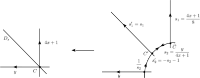
Figure 4. Fig.4 Blowing-up at $C$. For brevity of notation, $\tilde{C}$ is called $C$ again in the text.

7.1.b. Mirror map and Gromov-Witten invariants. Calculations of mirror map and Gromov-Witten invariants are parallel to the previous cases. In the present case the regular local solution $\omega_{0}^{C}(s)$ has the from

$$\omega_{0}^{C}(s)=1+8s_{1}+56s_{1}^{2}+384s_{1}^{3}+\cdots+s_{2}(-16s_{1}^{2}-256s_{1}^{3}-\cdots)+\cdots,$$

and we arrange all solutions into the canonical form $\Pi_{C}(s)$ in (C.2). Mirror map is described by

$$q_{1}=e^{\frac{\omega_{1}}{\omega_{0}}}=C_{1}s_{1}\,\exp\big{(}\frac{\omega_{1}^{reg}}{\omega_{0}}\big{)},\,\,\,\,q_{2}=e^{\frac{\omega_{2}}{\omega_{0}}}=C_{2}s_{2}\,\exp\big{(}\frac{\omega_{2}^{reg}}{\omega_{0}}\big{)},$$

in terms of $\omega_{0}=\omega_{0}^{C}$ and $\omega_{i}=\omega_{i}^{C}$ and some constants $C_{k}$. Inverting these, we have $s_{a}=s_{a}(q_{1},q_{2})$ for $a=1,2$. Then the quantum corrected Yukawa couplings are given by

(7.2) $$Y_{ijk}^{C}=\left(\frac{1}{N_{C}\omega_{0}^{C}}\right)^{2}\sum_{a,b,c}C_{abc}^{C}\frac{ds_{a}}{dt_{i}}\frac{ds_{b}}{dt_{j}}\frac{ds_{c}}{dt_{k}}.$$

Proposition 7.2.

When we set $N_{C}=\frac{1}{\sqrt{2}}$, and $C_{1}=\sqrt{-1},C_{2}=1$ in the definition of the mirror map, we have

$$Y_{111}^{C}=16+512q_{1}^{2}q_{2}+22528q_{1}^{4}q_{2}+\cdots, Y_{112}^{C}=8+256q_{1}^{2}q_{2}+5632q_{1}^{4}q_{2}+\cdots,$$

$$Y_{122}^{C}=128q_{1}^{2}q_{2}+1408q_{1}^{4}q_{2}+9216q_{1}^{6}q_{2}^{2}+\cdots, Y_{222}^{C}=8q_{2}+8q_{2}^{2}+8q_{2}^{3}+\cdots+64q_{1}^{2}q_{2}+.$$

We have exactly same form for the corresponding expansions of $Y_{ijk}^{C^{\prime}}$.

We observe in the above $q$-series expansions of $Y_{ijk}^{C}$ that non-vanishing coefficients appear only for even-powers of $q_{1}$.

$$\begin{array}[]{|c|ccccccccc}\hline\cr{}j\diagdown i{}&0&1&2&3&4&5&6&7&8\\ \hline\cr 0&0&0&0&0&0&0&0&0&0\\ 1&8&64&352&1536&5808&19712&61632&180224&498696\\ 2&0&0&512&12288&152576&1351680&9596928&58040320&310097920\\ 3&0&0&352&24384&787632&15603712&221577504&2470588416&22896066536\\ 4&0&0&0&12288&1320960&59842560&1654833152&32671129600&502295842816\\ 5&0&0&0&1536&787632&91112640&5099691008&179687448576&4551683595656\\ 6&0&0&0&0&152576&59842560&7345469952&476575268864&20119442417664\\ 7&0&0&0&0&5808&15603712&5099691008&654619035200&47548652073448\\ :&:&{}:&{}:&{}:&{}:&{}:&{}:&{}:&:\end{array}$$

(0) BPS numbers $n_{0}^{C}(i,j)$

$$\begin{array}[]{|c|cccccccc}\hline\cr{}j\diagdown i{}&0&1&2&3&4&5&6&7\\ \hline\cr 0&0&8&8&8&8&8&8&8\\ 1&0&96&1824&16384&104480&533120&2332608&9074688\\ 2&0&8&5072&216480&4207776&53459792&513205888&4022629824\\ 3&0&0&1824&462176&27062912&798811136&15453590048&222719072256\\ 4&0&0&8&216480&47771216&3439792064&134032422304&3481149295168\\ 5&0&0&0&16384&27062912&5471284128&449545296384&21314156435456\\ 6&0&0&0&8&4207776&3439792064&664078158608&60005323039296\\ 7&0&0&0&0&104480&798811136&449545296384&84043909825632\\ :&:&:&:&:&:&:&:&:\end{array}$$

(1) BPS numbers $n_{1}^{C}(i,j)$

Table 3. Table 3. BPS numbers $n_{g}^{C}(i,j)=n_{g}^{C}(\beta.H_{Z},\beta.A_{Z})$ of $Z=V_{8,w}^{1}/\mathbb{Z}_{8}$. These are equal to the corresponding $n_{g}^{C^{\prime}}(i,j)$ of $Z^{\prime}=V_{8,w}^{2}/\mathbb{Z}_{8}$.

7.2. Genus one potential $F_{1}^{C}$

We calculate genus one Gromov-Witten invariants by using BCOV formula (5.10).

7.2.a. BCOV potential function $F_{1}^{C}$. Let us introduce the following definitions:

$$disC_{0}=(1-4s_{1})^{4}+256s_{1}^{2}(1-8s_{1})s_{2}(1+s_{2}),$$

$$disC_{1}=1+s_{2},\,\,\,disC_{2}=1-4s_{1},\,\,\,disC_{3}=1-8s_{1}.$$

As in Subsection 5.7, knowing that the boundary point $C$ is mirror symmetric to a free quotient $V_{8,w}^{1}/\mathbb{Z}_{8}$, we can determine the parameters $r_{0}$ and $r_{k}$ contained in the BCOV formula.

Proposition 7.3.

Around the boundary point $C$, the BCOV potential function has the following form

$$F_{1}^{C}(q_{1},q_{2})=\frac{1}{2}\log\Big{\{}\big{(}\frac{1}{\omega_{0}^{C}}\big{)}^{5}\frac{\partial(s_{1},s_{2})}{\partial(t_{1},t_{2})}disC_{0}^{-\frac{8}{6}}\,disC_{1}^{-1}\,disC_{2}^{-1}\,disC_{3}^{-\frac{5}{3}}s_{1}^{-1-\frac{16}{12}}s_{2}^{-1}\Big{\}}.$$

Assuming mirror symmetry, we read the genus one Gromov-Witten invariants from these potential functions. In Table 3 (1), we have listed the resulting BPS numbers (see also 7.5 below). Also, from the from of $F_{1}^{C}$, it is easy to verify the following property:

Proposition 7.4.

The potential functions $F_{1}^{C}$ and $F_{1}^{A}$ are NOT related to each other on $\mathbb{P}_{\Delta}$ by the transformation rules $($t1$)$ and $($t2$)$ in $($6.5$)$.

We will interpret the above proposition in Subsection 7.4 (Proposition 7.9).

Remark 7.5.

Recall that the conifold factor of $F_{1}^{M}$ in Remark 5.11 counts the number of ODPs or vanishing $S^{3}$’s which appear over the principal component of the discriminant of a family. In many examples, it is observed that the conifold factor is generalized to vanishing lens space $S^{3}/\mathbb{Z}_{N}$ by counting $-\frac{N}{6}$ for each lens space $S^{3}/\mathbb{Z}_{N}$ (eg. [AM1],[HT13]). Based on this, we read the BCOV formula $F_{1}^{C}$ as the one applied for the family $\mathcal{V}_{\mathbb{Z}_{8}\times\mathbb{Z}_{8}}^{1}\rightarrow\mathbb{P}_{\Delta}$. In fact, we have one vanishing cycle $S^{3}$ in each fiber $V_{8,w}^{1}/\mathbb{Z}_{8}$ of the family $\mathcal{V}_{\mathbb{Z}_{8}}^{1}$ over $\left\{disC_{0}=0\right\}=\left\{dis_{0}=0\right\}$, i.e., the $\tau$-orbit in Proposition 3.6. This vanishing cycle gives rise to a lens space $S^{3}/\langle\sigma\rangle$ in the full quotient $\mathcal{V}_{\mathbb{Z}_{8}\times\mathbb{Z}_{8}}^{1}\rightarrow\mathbb{P}_{\Delta}$ by $\mathbb{Z}_{8}\times\mathbb{Z}_{8}=\langle\sigma,\tau\rangle.$ This explains the conifold factor in $disC_{0}^{-\frac{8}{6}}$ and also the claimed property in Proposition 7.4, because $F_{1}^{C}$ and $F_{1}^{A}$ are defined for different families $\mathcal{V}_{\mathbb{Z}_{8}\times\mathbb{Z}_{8}}^{1}$ and $\mathcal{V}_{\mathbb{Z}_{8}}^{1}$, respectively. $\hfill\square$

7.2.b. Generators of $H_{2}(V^{1}_{8,w}/\mathbb{Z}_{8})$. Recall that we fixed a subgroup $\mathbb{Z}_{8}=\langle\tau\rangle$ to define a quotient $V_{8,w}^{1}/\mathbb{Z}_{8}$. Since $V_{8,w}^{1}$ is simply connected, the fundamental group of the free quotient $V_{8,w}^{1}/\mathbb{Z}_{8}$ is isomorphic to $\mathbb{Z}_{8}$. In the same way as in 6.5, we can argue the generators of $H_{2}(V_{8,w}^{1}/\mathbb{Z}_{8},\mathbb{Z})$ from the exact sequence

$$1\rightarrow\pi_{2}(V_{8,w}^{1}/\mathbb{Z}_{8})\rightarrow H_{2}(V_{8w}^{1}/\mathbb{Z}_{8},\mathbb{Z})\rightarrow H_{2}(\mathbb{Z}_{8})\rightarrow 0,$$

where $H_{2}(\mathbb{Z}_{8})=H_{2}(\pi_{1}(V_{8,w}^{1}/\mathbb{Z}_{8}))$ is the group homology. Since $H_{2}(\mathbb{Z}_{8})=0$ this time, we see the isomorphism $\pi_{2}(V_{8,w}^{1}/\mathbb{Z}_{8})\simeq H_{2}(V_{8w}^{1}/\mathbb{Z}_{8},\mathbb{Z})$, which indicates that $H_{2}$ is generated by rational curves. In fact, we have generators as follows: Let us note that both $V_{8,w}^{1}$ and $V_{8,w}^{1}/\mathbb{Z}_{8}$ have fibrations by abelian surfaces. We take divisors $H_{X}$ and $A_{X}$ to be the restriction of the hyperplane class and the fiber class of $V_{8,w}^{1}(=X)$, respectively. Denote the free quotient by $\pi:V_{8,w}^{1}\rightarrow V_{8,w}^{1}/\mathbb{Z}_{8}=Z$. Since the free $\mathbb{Z}_{8}$-action acts on each fiber, we have $\pi^{*}A_{Z}=A_{X}$ for the pull-back of the fiber class $A_{Z}$ of $V_{8,w}^{1}/\mathbb{Z}_{8}$. The group $\mathbb{Z}_{8}$ acts diagonally on the coordinates $x_{i}$. Hence, restricting the divisor $\left\{x_{i}=0\right\}$ to $V_{8,w}^{1}$, we have a $\mathbb{Z}_{8}$-invariant divisor of the class $H_{X}$, which is the pull-back of a divisor $H_{Z}$ on $Z$. To summarize, we have

(7.3) $$\pi^{*}H_{Z}=H_{X},\,\,\,\,\,\pi^{*}A_{Z}=A_{X}.$$

Now, for these two divisors $H_{Y}$ and $A_{Y}$ on $V_{8,w}^{1}/\mathbb{Z}_{8}$, we calculate

$$1=H_{X}.\ell=H_{Z}.(\pi_{*}\ell), 0=H_{X}\cdot\sigma_{X}=H_{Z}.(\pi_{*}\sigma_{X}),$$

$$0=A_{X}.\ell=A_{Z}.(\pi_{*}\ell), 1=A_{X}.\sigma_{X}=A_{Z}.(\pi_{*}\sigma_{X}),$$

where $\sigma_{X}$ is a section of abelian surface fibration $V_{8,w}^{1}\rightarrow\mathbb{P}^{1}$ and $\ell$ is a line contained in a singular fiber of $V_{8,w}^{1}$ (see 2.2). These relations show that, modulo torsion elements, the classes of $\pi_{*}\ell$ and $\pi_{*}\sigma_{X}$ generate $H_{2}(V_{8,w}^{1}/\mathbb{Z}_{8},\mathbb{Z})\simeq\pi_{2}(V_{8,w}^{1}/\mathbb{Z}_{8})$ and also $H_{Z}$ and $A_{Z}$ generate $Pic(V_{8,w}^{1}/\mathbb{Z}_{8})$.

Note that, from (7.3), we can determine the following invariants of $Z{\color[rgb]{0,0,0}}=V_{8,w}^{1}/\mathbb{Z}_{8}$,

(7.4) $$H_{Z}^{3}=H_{Z}^{2}A_{Z}=2,\,\,\,\,H_{Z}A_{Z}^{2}=A_{Z}^{3}=0;\,\,\,\,\,\,c_{2}.H_{Z}=8,\,\,c_{2}.A_{Z}=0.$$

7.2.c. Gromow-Witten invariants from potential functions $F^{C}_{0},F^{C}_{1}$. Recall that Gromov-Witten potential $F_{0}^{C}(t_{1},t_{2})$ at genus $0$ is defined as a function which satisfies

$$Y_{ijk}^{C}=\frac{\partial^{3}\;}{\partial t_{i}\partial t_{j}\partial t_{k}}F^{C}(t_{1},t_{2})$$

for the quantum corrected Yukawa couplings in Proposition 7.2 with $q_{i}=e^{t_{i}}$. As a generating function of Gromov-Witten invariants, this function takes the following general form:

$$F_{0}(t_{1},t_{2})=\frac{1}{3!}\int_{Z}\kappa_{t}^{3}+\sum_{{\beta\in H_{2}(Y,\mathbb{Z})\atop\beta\not=0}}N_{0}(\beta)e^{\beta.\kappa_{t}}$$

with $\kappa_{t}:=t_{1}H_{1}+t_{2}H_{2}$ in terms of some nef-divisors $H_{i}$. Comparing the invariants in (7.4) with the constant terms of $Y_{ijk}^{C}$, we see that, for the potential function $F_{0}^{C}(t_{1},t_{2})$ from $Y_{ijk}^{C}$ in Proposition 7.2, we should have

(7.5) $$\kappa_{t}=t_{1}(2H_{Z})+t_{2}A_{Z}.$$

Once we know the above identification of divisors, the genus one Gromov-Witten invariants $N_{1}(\beta)$ are read by identifying the BCOV formula for $F_{1}^{C}$, up to a constant term, with the following general form:

$$F_{1}(t)=-\frac{c_{2}.\kappa_{t}}{24}+\sum_{{\beta\in H_{2}(Y,\mathbb{Z})\atop\beta\not=0}}N_{1}(\beta)e^{\beta.\kappa_{t}}.$$

The BPS numbers $n_{g}(i,j)=n_{g}(\beta.H_{Z},\beta.A_{Z})$ listed in Table 3 are determined from $N_{g}(\beta)=N_{g}(\beta.H_{Z},\beta.A_{Z})$ which are read from $F_{0}^{C}(t)$ and $F_{1}^{C}(t)$.

Remark 7.6.

When reading Gromov-Witten invariants from (5.6) and (6.4), we implicitly identified the $\kappa_{t}$ in the potential function with $\kappa_{t}=t_{1}H_{X}+t_{2}A_{X}$ and $\kappa_{t}=t_{1}H_{Y}+t_{2}A_{Y}$, respectively. We note that $H_{X},A_{X}$ and $H_{Y},A_{Y}$ in these equations are generators of the Picard groups, while $2H_{Z},A_{Z}$ in (7.5) are not. The above example shows that a non-trivial identification of $\kappa_{t}$ like (7.5) introduces a slight subtlety when reading $N_{g}(\beta)$ from the potential functions $F_{g}(t)$ which we calculate by using mirror symmetry. $\hfill\square$

7.2.d. $Z_{g,n}(q)$ by modular forms. We define the $q$-series $Z_{g,n}^{C}(q)$ from the potential functions $F_{g}^{C}(q,p)$ as in the preceding sections. From Table 3, it is easy to observe that

(7.6) $$Z_{0,1}^{C}(q)=\frac{8}{\bar{\eta}(q^{2})^{8}},$$

where $q^{2}$ comes from the relation (7.5). Also, corresponding to (6.7), we find the following relations:

$$P_{0,n}^{C}(q)=8^{n-1}P_{0,n}^{A}(q^{2})\,\,\,\,(n\geq 1),$$

for the polynomials defined by $Z_{g,n}^{C}(q)=P_{g,n}^{C}(q)\left(\frac{8}{\bar{\eta(q^{2})^{8}}}\right)^{n}$. Furthermore, at $g=1$, we can calculate explicitly the following forms of $P_{1,n}^{C}(q)$ in terms of elliptic quasi-modular forms $\tilde{E}_{k}:=E_{k}(q^{2})\,(k=2,4,6)$ for lower $n$ (see also [HT21]):

$$P_{1,1}^{C}= \frac{1}{36}(\tilde{E}_{2}^{2}+2\tilde{E}_{4}),$$

$$P_{1,2}^{C}= \frac{1}{10368}(8\tilde{E}_{2}^{4}+13\tilde{E}_{2}^{2}\tilde{E}_{4}+17\tilde{E}_{2}\tilde{E}_{6}+16\tilde{E}_{4}^{2}),$$

$$P_{1,3}^{C}= \frac{1}{2^{14}3^{7}}(1048\tilde{E}_{2}^{6}+1995\tilde{E}_{2}^{4}\tilde{E}_{4}+3642\tilde{E}_{2}^{2}\tilde{E}_{4}^{2}+1711\tilde{E}_{4}^{3}+2444\tilde{E}_{2}^{3}\tilde{E}_{6}$$

$${\hskip 170.0pt}+3948\tilde{E}_{2}\tilde{E}_{4}\tilde{E}_{6}+764\tilde{E}_{6}^{2}).$$

7.2.e. Contraction to $(2,2,2,2)/\mathbb{Z}_{8}$. Birational geometry of $V_{8,w}^{1}/\mathbb{Z}_{8}$ is quite parallel to the cases of $V_{8,w}^{1}$ and $V_{8,w}^{1}/\mathbb{Z}_{8}\times\mathbb{Z}_{8}$; the diagram (5.8) is valid with the free $\mathbb{Z}_{8}$ actions;

(7.7) $$\begin{matrix}\lx@xy@svg{\hbox{\raise 0.0pt\hbox{\kern 61.06226pt\hbox{{\hbox{\kern-61.06226pt\raise 0.0pt\hbox{\hbox{\kern 6.0pt\raise-2.87222pt\hbox{$\textstyle{V^{1}_{8,w}/\mathbb{Z}_{8}}$}}}}}{\hbox{\kern 24.29556pt\raise 0.0pt\hbox{\hbox{\kern 6.0pt\raise-2.87222pt\hbox{$\textstyle{V^{2}_{8,w}/\mathbb{Z}_{8}}$}}}}}{\hbox{\kern-25.42361pt\raise-36.98839pt\hbox{\hbox{\kern 6.0pt\raise-2.89333pt\hbox{$\textstyle{X_{2,2,2,2}^{sing}/\mathbb{Z}_{8}}$}}}}}{\hbox{\kern-41.86005pt\raise-19.91682pt\hbox{\hbox{\kern 6.0pt\raise-3.5pt\hbox{$\textstyle{\,{}^{\,{}_{8\,\mathbb{P}^{1}}}}$}}}}}{\hbox{\kern 20.73569pt\raise-19.91682pt\hbox{\hbox{\kern 6.0pt\raise-3.5pt\hbox{$\textstyle{\,{}^{\,{}_{8\,\mathbb{P}^{1}}}}$}}}}}\ignorespaces\ignorespaces\ignorespaces\ignorespaces{\hbox{\kern-24.29556pt\raise 0.0pt\hbox{\hbox{\kern 0.0pt\raise 0.0pt\hbox{\lx@xy@tip{1}\lx@xy@tip{-1}}}}}}\ignorespaces\ignorespaces\ignorespaces{\hbox{\lx@xy@drawline@}}\ignorespaces\ignorespaces{\hbox{\kern-3.0pt\raise 0.0pt\hbox{{}\hbox{\kern 0.0pt\raise 0.0pt\hbox{\hbox{\kern 3.0pt\hbox{\hbox{\kern 0.0pt\raise 0.0pt\hbox{$\scriptstyle{}$}}}\kern 3.0pt}}}}}}\ignorespaces{\hbox{\kern 24.29556pt\raise 0.0pt\hbox{\hbox{\kern 0.0pt\raise 0.0pt\hbox{\lx@xy@tip{1}\lx@xy@tip{-1}}}}}}\ignorespaces\ignorespaces\ignorespaces{\hbox{\lx@xy@drawline@}}\ignorespaces{\hbox{\lx@xy@drawline@}}\ignorespaces\ignorespaces\ignorespaces\ignorespaces\ignorespaces{}\ignorespaces\ignorespaces\ignorespaces{\hbox{\lx@xy@drawline@}}\ignorespaces{\hbox{\kern-13.59378pt\raise-25.20174pt\hbox{\hbox{\kern 0.0pt\raise 0.0pt\hbox{\lx@xy@tip{1}\lx@xy@tip{-1}}}}}}\ignorespaces\ignorespaces\ignorespaces{\hbox{\lx@xy@drawline@}}\ignorespaces{\hbox{\lx@xy@drawline@}}\ignorespaces\ignorespaces\ignorespaces\ignorespaces\ignorespaces{}\ignorespaces\ignorespaces\ignorespaces{\hbox{\lx@xy@drawline@}}\ignorespaces{\hbox{\kern 13.60529pt\raise-25.20174pt\hbox{\hbox{\kern 0.0pt\raise 0.0pt\hbox{\lx@xy@tip{1}\lx@xy@tip{-1}}}}}}\ignorespaces\ignorespaces\ignorespaces{\hbox{\lx@xy@drawline@}}\ignorespaces{\hbox{\lx@xy@drawline@}}\ignorespaces}}}}\end{matrix} \textstyle{V^{1}_{8,w}/\mathbb{Z}_{8}} \textstyle{V^{2}_{8,w}/\mathbb{Z}_{8}} \textstyle{X_{2,2,2,2}^{sing}/\mathbb{Z}_{8}} \textstyle{\,{}^{\,{}_{8\,\mathbb{P}^{1}}}} \textstyle{\,{}^{\,{}_{8\,\mathbb{P}^{1}}}} \textstyle{V^{1}_{8,w}/\mathbb{Z}_{8}} \textstyle{V^{2}_{8,w}/\mathbb{Z}_{8}} \textstyle{X_{2,2,2,2}^{sing}/\mathbb{Z}_{8}} \textstyle{\,{}^{\,{}_{8\,\mathbb{P}^{1}}}} \textstyle{\,{}^{\,{}_{8\,\mathbb{P}^{1}}}}$$

The birational model $V_{8,w}^{2}/\mathbb{Z}_{8}$ corresponds to the other boundary point $C^{\prime}$ in Fig.4. We note that the singular Calabi-Yau complete intersection $X_{2,2,2,2}^{sing}/\mathbb{Z}_{8}$ admits a smoothing to a smooth free quotient $X_{2,2,2,2}/\mathbb{Z}_{8}$ in [Br, Hu]. We can observe the following sum-up properties for $g=0$ and $g=1$ BPS numbers:

(7.8) $$\sum_{d_{2}}n_{0}^{C}(d,d_{2})=\frac{1}{|\mathbb{Z}_{8}|}n_{0}^{(2,2,2,2)}(d),\,\,\,\,\sum_{d_{2}}n_{1}^{C}(d,d_{2})=n_{1}^{(2,2,2,2)/\mathbb{Z}_{8}}(d).$$

The number $\frac{1}{|\mathbb{Z}_{8}|}n_{0}^{(2,2,2,2)}(d)$ can be interpreted as BPS numbers of the smooth free quotient $X_{2,2,2,2}/\mathbb{Z}_{8}$. The number $n_{1}^{(2,2,2,2)/\mathbb{Z}_{8}}(d)$ has been determined in Appendix E.3 from BCOV formula assuming a mirror family of the smooth free quotient $X_{2,2,2,2}/\mathbb{Z}_{8}$.

7.3. Genus two potential $F_{2}^{C}$ and $F_{g}^{C}\,(g\geq 2)$.

It is quite parallel to the cases of $F_{2}^{A}$ and $F_{2}^{B}$ to determine the genus two potential function $F_{2}^{C}$ up to a rational function $f_{2}^{C}(s_{1},s_{2})$. It is easy to find a suitable ansatz on $f_{2}^{C}$ and impose the most reasonable vanishing conditions on some BPS numbers; however, there still remain undetermined parameters. If $F_{2}^{C}$ were related to $F_{2}^{A}$ or $F_{2}^{B}$ on $\mathbb{P}_{\Delta}$ by the transformation rules (t1)^′ and (t2)^′, then $f_{2}^{C}$ would be determined from $f_{2}^{A}$. However, we find that vanishing conditions for $A$ and $C$ are not compatible, i.e., we encounter non-integral BPS numbers if we impose them. At genus one, we have already encountered the corresponding situation in Proposition 7.4.

Our verifications of the following conjecture are restricted to genus zero and one; but we expect that it holds in general because BCOV recursion formulas for $F_{g}(g\geq 2)$ start with $F_{0}$ and $F_{1}$ as initial data.

Conjecture 7.7.

The $q$-series $Z_{g,n}^{C}(q)$ of Gromov-Witten invariants of $V_{8,w}^{1}/\mathbb{Z}_{8}$ are written by quasi-modular modular forms as

$$Z_{g,n}^{C}(q)=P_{g,n}^{C}(E_{2}(q^{2}),E_{4}(q^{2}),E_{6}(q^{2}))\left(\frac{8}{\bar{\eta}(q^{2})^{8}}\right)^{n},$$

where $P_{g,n}^{C}(E_{2}(q^{2}),E_{4}(q^{2}),E_{6}(q^{2}))$ are quasi-modular forms of weight $4(g+n-1)$.

Remark 7.8.

In physics, the whole set $\left\{F_{g}^{M}\right\}$ of potential functions define the so-called topological string theory on a Calabi-Yau manifold $M$. From the above (conjectural) simple structure on $P_{g,n}^{C}$, we may naturally expect that the topological string on $Z=V_{8,w}^{1}/\mathbb{Z}_{8}$ is completely integrable, i.e., the whole set $\left\{F_{g}^{M}\right\}$ may be determined completely. Mathematically, the simplification in the quasi-modular property of $Z_{g,n}^{C}(q)$ may be explained by the fact that the fiber abelian surfaces are principally polarized for the fibration $V_{8,w}^{1}/\mathbb{Z}_{8}\rightarrow\mathbb{P}^{1}$ as we see in (7.4). $\hfill\square$

7.4. Mirror symmetry

In Section 5, with a subgroup $\mathbb{Z}_{8}=\langle\tau\rangle\subset\mathbb{Z}_{8}\times\mathbb{Z}_{8}$, we have introduced two families

$$\mathfrak{X}=\mathcal{V}_{\mathbb{Z}_{8}}^{1}\rightarrow\mathbb{P}_{\Delta}\,\,\text{and }\,\,\mathfrak{X}=\mathcal{V}_{\mathbb{Z}_{8}\times\mathbb{Z}_{8}}^{1}\rightarrow\mathbb{P}_{\Delta}$$

over the same parameter space $\mathbb{P}_{\Delta}$. The local systems $R^{3}\pi_{*}\mathbb{C}_{\mathfrak{X}}$ associated to these are represented by the same Picard-Fuchs differential equations $\mathcal{D}_{2}\omega=\mathcal{D}_{3}\omega=0$ (5.3) on $\mathbb{P}_{\Delta}$. We can now summarize our results from each boundary point of $A,B;A^{\prime},B^{\prime};C,C^{\prime}$ as follows.

Proposition 7.9.

The following two different pictures of mirror symmetry are encoded in the same Picard-Fuchs differential equations $($5.3$)$ :

• $(1)$ When we read $($5.3$)$ as representing the local system of the family $\mathcal{V}_{\mathbb{Z}_{8}}^{1}\rightarrow\mathbb{P}_{\Delta}$, mirror symmetry of the family to Calabi-Yau manifolds $V_{8,w}^{1}$ and $V_{8,w}^{1}/\mathbb{Z}_{8}\times\mathbb{Z}_{8}$ are identified at the boundary points $A$ and B, respectively. Mirror symmetry to birational models $V_{8,w}^{2}$ and $V_{8,w}^{2}/\mathbb{Z}_{8}\times\mathbb{Z}_{8}$ are also identified at $A^{\prime}$ and $B^{\prime}$.

• $(2)$ When we read $($5.3$)$ as representing the local system of the family $\mathcal{V}_{\mathbb{Z}_{8}\times\mathbb{Z}_{8}}^{1}\rightarrow\mathbb{P}_{\Delta}$, mirror symmetry of the family to a Calabi-Yau manifold $V_{8,w}^{1}/\mathbb{Z}_{8}$ is identified at the boundary point C. Mirror symmetry to the birational model $V_{8,w}^{2}/\mathbb{Z}_{8}$ is identified at $C^{\prime}$.

At this moment, our identifications of the mirror families $\mathcal{V}_{\mathbb{Z}_{8}}^{1}$ and $\mathcal{V}_{\mathbb{Z}_{8}\times\mathbb{Z}_{8}}^{1}$ as above are based on the genus one potential functions $F_{1}^{A},F_{1}^{B}$ and $F_{1}^{C}$ (Remarks 5.11 and 7.5). In the next section (Proposition 8.3), the difference between the two families will be explained further by integral structures from the solutions of (5.3).

The above proposition is our affirmative answer to Conjecture 1.1.

Remark 7.10.

Calabi-Yau manifolds $V_{8,w}^{1}$ and $V_{8,w}^{1}/\mathbb{Z}_{8}\times\mathbb{Z}_{8}$ are Fourier-Mukai partners to each other. The above proposition shows that they are mirror symmetric to the family $\mathcal{V}_{\mathbb{Z}_{8}}^{1}\rightarrow\mathbb{P}_{\Delta}$. Conversely, Calabi-Yau manifold $V_{8,w}^{1}/\mathbb{Z}_{8}$ should be mirror symmetric to both the family $\mathcal{V}_{\mathbb{Z}_{8}\times\mathbb{Z}_{8}}^{1}\rightarrow\mathbb{P}_{\Delta}$ and a family of $V_{8,w}^{1}$ over some parameter space, although we haven’t constructed the latter.$\hfill\square$

8. Degenerations and analytic continuations

We further study our results in Proposition 7.9 by calculating the connection matrices for the local solutions at each boundary point $A,B$ and $C$. We also describe the degenerations of Calabi-Yau manifolds over these points. We expect that categorical and geometric aspects of mirror symmetry, including Fourier-Mukai partners, will appear in explicit and concrete forms from these degenerations, but we leave the details for future investigations.

8.1. Analytic continuations of period integrals

We consider the connection problem of local solutions around the boundary points $A,B$ and $C$ of the Picard-Fuchs differential equations (5.3). To set up the connection problem, we arrange local solutions into the canonical form (C.2) in Appendix C; and write them by

$$\Pi_{A}(x,y),\,\,\,\Pi_{B}(z_{1},z_{2}),\,\,\,\Pi_{C}(s_{1},s_{2}),$$

where we use the affine coordinates centered at each boundary point which are related to each other by (6.1) and (7.1). Here we set the parameters $a_{ij}$ to zero in the canonical forms $\Pi_{P}$ for all $P=A,B,C$ (and $\tilde{A}$). To simplify our calculations, in this paper, we will restrict our calculations for the above three points (and $\tilde{A}$ additionally).

8.1.a. Making local solutions. To do analytic continuations, we need to generate local solutions in the forms of power series up to sufficiently high degrees. In the present case, the following property of the Picard-Fuchs system enables us to do it efficiently. Below we sketch our calculations for the case $A$, but calculations for other cases $B,C$ and also $\tilde{A}$ are quite parallel.

Let us recall the forms of local solutions $\omega_{0}(x),\omega_{i}(x),\omega_{2,i}(x),\omega_{3}(x)$ in (C.1). Arrange the regular solution $\omega_{0}(x)$ by powers of $y$,

$$\omega_{0}(x,y)=f_{0}(x)+f_{1}(x)y+f_{2}(x)y^{2}+f_{3}(x)y^{3}\cdots,$$

and substitute this into $\mathcal{D}_{2}\omega_{0}=0$, then we obtain polynomial relations

$$f_{n}+G_{n}(x,f_{n-1},f_{n-1}^{\prime},f_{n-1}^{\prime\prime})=0\,\,\,\,(n=1,2,\cdots),$$

which we can solve recursively with an initial data $f_{0}(x)$. From $\mathcal{D}_{2}\omega_{0}=\mathcal{D}_{3}\omega_{0}=0,$ it is easy to find the initial data $f_{0}(x)=\sum_{n\geq 0}\frac{(2n)!(2n)!}{(n!)^{4}}x^{2n}$. Basically, this method works for other local solutions assuming their forms in (C.1). For the case of $\omega_{1}$, for example, having $\omega_{0}(x)$ up to desired orders in $x$ and $y$, arrange $\omega_{1}(x)$ as

$$\omega_{1}(x,y)=\omega_{0}(x,y)\log x+g_{0}(x)+g_{1}(x)y+g_{2}(x)y^{2}+\cdots,$$

and substitute this into $\mathcal{D}_{2}\omega_{1}=0$. Then we obtain polynomial relations

$$g_{n}+K_{n}(x,g_{n-1},g_{n-1}^{\prime},g_{n-1}^{\prime\prime})=0\,\,\,\,(n=1,2,\cdots),$$

which we can solve recursively once we determine $g_{0}(x)$. To determine $g_{0}(x)$, we use the equations $\mathcal{D}_{2}\omega_{1}=\mathcal{D}_{3}\omega_{1}=0$ to find a linear differential equation of $g_{0}(x)$ described by the data $f_{0}(x)$ and $f_{1}(x)$.

Though the solutions $\omega_{2,i}(x),\omega_{3}(x)$ contain polynomials of higher powers of $\log x$ and $\log y$, we can continue the same process after having solutions $\omega_{0}(x)$ and $\omega_{i}(x)$.

8.1.b. Connection matrices. Analytic continuation of local solutions is tedious in general for differential equations of multi-variables. However, note that the boundary points $A,B,C$ and $A^{\prime}$ are aligned on the real line of a single rational boundary divisor in $\mathbb{P}_{\Delta}$ (see Fig.5). This reduces our connection problem essentially to that of one variable. In fact, we can obtain the following results by making local solutions up to the first order in $y$ but sufficiently higher order in $x$.

To describe the results, let us write by $\Pi_{A}(x),\Pi_{B}(z),\Pi_{\tilde{A}}(\tilde{x})$ and $\Pi_{C}(s)$ the local solutions in the canonical form (C.2) with $a_{ij}=0$ for $A,B,\tilde{A}$ and $C$, respectively. Four points $A,B,\tilde{A}$ and $C$ are aligned on the real coordinate line of a boundary divisor $\left\{y=0\right\}$ with their coordinates $(x,0)=(0,0),(\frac{1}{4},0),(\infty,0)$ and $(-\frac{1}{4},0)$ in order. We define connection matrices along the real coordinate line (see Fig.5) by

$$\Pi_{A}=U_{AB}\Pi_{B},\,\,\,\,\Pi_{B}=U_{B\tilde{A}}\Pi_{\tilde{A}},\,\,\,\,\,\Pi_{\tilde{A}}=U_{\tilde{A}C}\Pi_{C},\,\,\,\,\,\Pi_{C}=U_{CA}\Pi_{A},$$

where $U_{PQ}$ represents the connection matrix of the analytic continuation of $\Pi_{P}$ to the point $Q$ along a path $P\rightarrow Q$ shown in Fig.5. Note that the canonical forms $\Pi_{P}$ of local solutions contain normalization constants $N_{P}$.

Proposition 8.1.

When we normalize the local solutions by

$$N_{A}=1,\,\,\,\,N_{B}=\frac{1}{2},\,\,\,\,N_{C}=\frac{1}{\sqrt{2}},\,\,\,\,N_{\tilde{A}}=2^{4},$$

then the connection matrices are represented by symplectic matrices with respect to $\Sigma$ in (C.3); explicitly, they are given by

$$U_{AB}=\left(\begin{matrix}\,\,0&0&0&{}{}-1&0&0\\ \,\,0&1&0&0&0&0\\ \,\,0&0&0&0&0&1\\ {}{}\,-1&0&0&0&0&0\\ \,\,0&0&0&0&1&0\\ \,\,0&0&1&0&0&0\end{matrix}\right),\,\,\,\,U_{\tilde{A}C}=\frac{1}{\sqrt{2}}\left(\begin{matrix}-2&8&0&{}{}-2&0&0\\ \,\,\frac{1}{2}&{}{}-3&0&1&0&0\\ \,\,\frac{3}{2}&{}{}-3&{}{}-2&0&1&2\\ -1&8&0&{}{}-4&0&0\\ -3&0&8&0&{}{}-6&{}{}-16\\ -\frac{5}{2}&10&1&{}{}-4&{}{}-1&{}{}-4\end{matrix}\right),$$

$$U_{B\tilde{A}}=\left(\begin{matrix}\,\,0&0&0&{}{}-1&0&0\\ \,\,0&1&0&\frac{1}{2}&0&0\\ \,\,0&0&0&2&0&1\\ {}{}\,-1&{}{}-8&0&{}{}-2&0&0\\ \,\,0&{}{}-96&0&{}{}-32&1&{}{}-8\\ {}{}\,-2&{}{}-32&1&{}{}-7&\frac{1}{2}&{}{}-2\end{matrix}\right),U_{CA}=\frac{1}{\sqrt{2}}\left(\begin{matrix}{}{}\,-4&16&0&{}{}-2&0&0\\ {}{}\,-1&2&0&0&0&0\\ \,\,4&0&{}{}-4&0&1&2\\ {}{}\,-1&0&0&0&0&0\\ \,\,6&{}{}-16&{}{}-8&1&1&0\\ \,\,\frac{1}{2}&{}{}-1&1&0&0&0\end{matrix}\right).$$

Remark 8.2.

(1) The values of the normalization constants $N_{P}$ are exactly the same as those used in (5.6),(6.4) and (7.2) to have right quantum corrected Yukawa couplings with right normalizations. (2) An ordered product of the above connection matrices represents a trivial loop on the divisor $\left\{y=0\right\}\simeq\mathbb{P}^{1}$. We observe that our choice of path for this loop is twisted by the monodromy $\log y\mapsto\log y-4\times 2\pi\sqrt{-1}$;

$$U_{AB}U_{B\tilde{A}}U_{\tilde{A}C}U_{CA}=\left(\begin{smallmatrix}1&0&0&0&0&0\\ 0&1&0&0&0&0\\ {}-1&0&1&0&0&0\\ 0&0&0&1&0&0\\ 0&{}-16&0&0&1&0\\ 0&0&0&1&0&1\end{smallmatrix}\right)^{4}.$$

This twist may be explained by the fact that we have resolved 4-th order tangency at the intersection point $B$ of $\left\{y=0\right\}$ and $\left\{dis_{0}=0\right\}$. $\hfill\square$

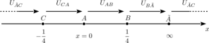
Figure 5. Fig.5

8.1.c. Integral and symplectic structures. As summarized in Appendix C, mirror symmetry arises from Picard-Fuchs differential equations of a family in the canonical forms $\Pi_{P}$ of local solutions at special boundary points $P$. It is conjectured in general [Hos1, Hos2] that the canonical form $\Pi_{P}$ introduces an integral and symplectic structure on the space of solutions which are compatible with mirror symmetry (see [GI] for a generalization to Fano varieties). Here, to go into further implications of mirror symmetry, let us assume this conjecture and denote by $\mathcal{H}_{\mathbb{Z},P}\simeq\mathbb{Z}^{6}$ the integral structure generated by the local solutions $\Pi_{P}$. As described in Appendix C, the solutions in $\Pi_{P}$ introduce a symplectic basis of $H_{3}$,

(8.1) $$\left\{\gamma_{k}^{P}\right\}=\left\{\alpha_{0}^{P},\alpha_{1}^{P},\alpha_{2}^{P},\beta_{2}^{P},\beta_{1}^{P},\beta_{0}^{P}\right\}$$

with $\langle\alpha_{i}^{P},\beta_{j}^{P}\rangle=-\langle\beta_{j}^{P},\alpha_{i}^{P}\rangle=\delta_{ij}$. We note that the connection matrix $U_{AB}$ in Proposition 8.1 is symplectic and integral, while $U_{CA}$ is symplectic but not integral. From this, we observe the following

Proposition 8.3.

The integral structures $\mathcal{H}_{\mathbb{Z},A}$ and $\mathcal{H}_{\mathbb{Z},B}$ are isomorphic to each other, while they are not isomorphic to $\mathcal{H}_{\mathbb{Z},C}$.

In Proposition 7.9, three boundary points $A,B,C$ are grouped into $A,B$ and $C$ from the transformation properties (connection properties) of the higher genus potential functions at $g=1$ and $2$. Combining this with the above result, we deduce again that the integral structure $\mathcal{H}_{\mathbb{Z},A}\simeq\mathcal{H}_{\mathbb{Z},B}$ comes from the local system $R^{3}\pi_{*}\mathbb{Z}_{\mathfrak{X}}$ associated with the family $\mathfrak{X}=\mathcal{V}_{\mathbb{Z}_{8}}^{1}\rightarrow\mathbb{P}_{\Delta}$, while $\mathcal{H}_{\mathbb{Z},C}$ comes from that of the other family $\mathfrak{X}=\mathcal{V}_{\mathbb{Z}_{8}\times\mathbb{Z}_{8}}^{1}\rightarrow\mathbb{P}_{\Delta}$.

Our result shows that BCOV theory of higher genus potential functions $F_{g}$ (topological string for physicists) depends on the integral structure $R^{3}\pi_{*}\mathbb{Z}_{\mathfrak{X}}$ although it is encoded in the theory in an implicit way. It is argued in physics that a topological string $\left\{F_{g}^{M}\right\}$ is equivalent to a wave function of a quantum mechanical system on $H^{3}(M,\mathbb{C})$ with the natural symplectic structure on $H^{3}(M,\mathbb{Z})$ (see e.g. [W, ABK]). We expect that our examples motivate investigations towards a global mathematical theory of these interesting ideas as well as BCOV recursion formulas.

Remark 8.4.

In the above proposition, we have excluded the boundary point $\tilde{A}$ from our consideration. This is because $A$ and $\tilde{A}$ are related by an involutive symmetry (4.3), which actually is a symmetry of the Picard-Fuchs differential equations. One may start all our calculations with $\tilde{A}$ and obtain the same results, e.g. Proposition 8.1, with $A$ replaced by $\tilde{A}$.$\hfill\square$

8.1.d. Derived equivalence and mirror symmetry. The mirror Calabi-Yau manifolds for the boundary points $A$ and $B$ are identified, respectively, with $V_{A}:=V_{8,w}^{1}$ and $V_{B}:=V_{8,w}^{1}/\mathbb{Z}_{8}\times\mathbb{Z}_{8}$, which are derived equivalent. The equivalence is described by the fiberwise Fourier-Mukai transformation [Ba, Sch]. In the mirror side, i.e. in the family of $\mathcal{V}_{\mathbb{Z}_{8}}^{1}\rightarrow\mathbb{P}_{\Delta}$, we can read this Fourier-Mukai transformation in the form of the connection matrix $U_{AB}$.

Let us recall that, under homological mirror symmetry [Ko], the integral symplectic structure $(\mathcal{H}_{\mathbb{Z},A},\left\{\gamma_{k}^{A}\right\})\simeq(\mathcal{H}_{\mathbb{Z},B},\left\{\gamma_{k}^{B}\right\})$ from the boundary points is transformed to the corresponding integral symplectic structures on the Grothendieck group $K(V_{A})\simeq K(V_{B})$ of coherent sheaves (see e.g. [Hos2]). Note that the isomorphism follows from the derived equivalence $D^{b}(V_{A})\simeq D^{b}(V_{B})$, and there the symplectic structure is naturally introduced by $\chi(\mathcal{E},\mathcal{F})=\sum_{i}(-1)^{i}\dim Ext^{i}(\mathcal{E},\mathcal{F})$. Mirror symmetry predicts that there are integral symplectic bases $\left\{\mathcal{E}_{\gamma_{k}}^{A}\right\},\left\{\mathcal{E}_{\gamma_{k}}^{B}\right\},$ which are mirror duals to the bases $\left\{\gamma_{k}^{A}\right\}$ and $\left\{\gamma_{k}^{B}\right\}$, respectively. Not so much is known about the integral symplectic basis $\left\{\mathcal{E}_{\gamma_{k}}\right\}$; however, for the symplectic basis (8.1) coming from the canonical form of period integrals $\Pi_{P}$, it is expected that the following naive correspondences hold:

(8.2) $$\left\{\gamma_{k}\right\}=\left\{\alpha_{0},\alpha_{1},\alpha_{2},\beta_{2},\beta_{1},\beta_{0}\right\}\underset{\text{\text{MD}}}{\longleftrightarrow}\left\{\mathcal{O}_{p},\mathcal{O}_{C_{1}},\mathcal{O}_{C_{2}},\mathcal{O}_{D_{2}},\mathcal{O}_{D_{1}},\mathcal{O}_{V}\right\}=\left\{\mathcal{E}_{\gamma_{k}}\right\},$$

where $\mathcal{O}_{p},\mathcal{O}_{V}$ are the skyscraper sheaf supported on $p\in V$ and the structure sheaf of a mirror Calabi-Yau manifold $V$, respectively. $\mathcal{O}_{C_{i}},\mathcal{O}_{D_{i}}$ are torsion sheaves supported on curves $C_{i}$ and dual divisors $D_{i}$. More precisely, we need suitable twists on these sheaves, but we omit these details for simplicity.

Assuming the above mirror duality (MD), we read the connection matrix $U_{AB}$ as in the following diagram:

(8.3) $$\begin{matrix}\lx@xy@svg{\hbox{\raise 0.0pt\hbox{\kern 161.28642pt\hbox{{\hbox{\kern-161.28642pt\raise 0.0pt\hbox{\hbox{\kern 6.0pt\raise-2.5pt\hbox{$\textstyle{\left\{\gamma_{k}^{A}\right\}=}$}}}}}{\hbox{\kern-127.8462pt\raise 0.0pt\hbox{\hbox{\kern 3.0pt\raise-2.5pt\hbox{$\textstyle{\{}$}}}}}{\hbox{\kern-25.57156pt\raise 0.0pt\hbox{\hbox{\kern 6.0pt\raise-2.5pt\hbox{$\textstyle{\}}$}}}}}{\hbox{\kern-122.79782pt\raise 0.0pt\hbox{\hbox{\kern 3.0pt\raise-1.18056pt\hbox{$\textstyle{\alpha_{0},}$}}}}}{\hbox{\kern-105.72626pt\raise 0.0pt\hbox{\hbox{\kern 3.0pt\raise-1.18056pt\hbox{$\textstyle{\alpha_{1},}$}}}}}{\hbox{\kern-85.6547pt\raise 0.0pt\hbox{\hbox{\kern 0.0pt\raise-1.18056pt\hbox{$\textstyle{\alpha_{2},}$}}}}}{\hbox{\kern-65.3675pt\raise 0.0pt\hbox{\hbox{\kern 0.0pt\raise-2.5pt\hbox{$\textstyle{\beta_{2},}$}}}}}{\hbox{\kern-48.29593pt\raise 0.0pt\hbox{\hbox{\kern 0.0pt\raise-2.5pt\hbox{$\textstyle{\beta_{1},}$}}}}}{\hbox{\kern-29.83546pt\raise 0.0pt\hbox{\hbox{\kern 0.0pt\raise-2.5pt\hbox{$\textstyle{\beta_{0}}$}}}}}{\hbox{\kern 12.99419pt\raise 0.0pt\hbox{\hbox{\kern 3.0pt\raise-2.5pt\hbox{$\textstyle{\{}$}}}}}{\hbox{\kern 143.72144pt\raise 0.0pt\hbox{\hbox{\kern 6.0pt\raise-2.5pt\hbox{$\textstyle{\}}$}}}}}{\hbox{\kern 18.76607pt\raise 0.0pt\hbox{\hbox{\kern 3.0pt\raise-2.26944pt\hbox{$\textstyle{\mathcal{O}_{p},}$}}}}}{\hbox{\kern 40.73541pt\raise 0.0pt\hbox{\hbox{\kern 3.0pt\raise-2.44444pt\hbox{$\textstyle{\mathcal{O}_{C},}$}}}}}{\hbox{\kern 67.09903pt\raise 0.0pt\hbox{\hbox{\kern 0.0pt\raise-2.44444pt\hbox{$\textstyle{\mathcal{O}_{\sigma},}$}}}}}{\hbox{\kern 89.36107pt\raise 0.0pt\hbox{\hbox{\kern 0.0pt\raise-2.44444pt\hbox{$\textstyle{\mathcal{O}_{A},}$}}}}}{\hbox{\kern 111.82721pt\raise 0.0pt\hbox{\hbox{\kern 0.0pt\raise-2.44444pt\hbox{$\textstyle{\mathcal{O}_{D},}$}}}}}{\hbox{\kern 136.11858pt\raise 0.0pt\hbox{\hbox{\kern 0.0pt\raise-2.45999pt\hbox{$\textstyle{\mathcal{O}_{V}}$}}}}}{\hbox{\kern-127.8462pt\raise-42.67891pt\hbox{\hbox{\kern 3.0pt\raise-2.5pt\hbox{$\textstyle{\{}$}}}}}{\hbox{\kern-22.7263pt\raise-42.67891pt\hbox{\hbox{\kern 6.0pt\raise-2.5pt\hbox{$\textstyle{\}}$}}}}}{\hbox{\kern-161.28642pt\raise-42.67891pt\hbox{\hbox{\kern 6.0pt\raise-2.5pt\hbox{$\textstyle{\left\{\gamma_{k}^{B}\right\}=}$}}}}}{\hbox{\kern-122.35992pt\raise-42.67891pt\hbox{\hbox{\kern 3.0pt\raise-2.5pt\hbox{$\textstyle{-\beta_{2},}$}}}}}{\hbox{\kern-100.03574pt\raise-42.67891pt\hbox{\hbox{\kern 3.0pt\raise-1.18056pt\hbox{$\textstyle{\alpha_{1},}$}}}}}{\hbox{\kern-85.43906pt\raise-42.67891pt\hbox{\hbox{\kern 3.0pt\raise-2.5pt\hbox{$\textstyle{\beta_{0},}$}}}}}{\hbox{\kern-71.51563pt\raise-42.67891pt\hbox{\hbox{\kern 3.0pt\raise-1.18056pt\hbox{$\textstyle{-\alpha_{0},}$}}}}}{\hbox{\kern-48.45067pt\raise-42.67891pt\hbox{\hbox{\kern 3.0pt\raise-2.5pt\hbox{$\textstyle{\beta_{1},}$}}}}}{\hbox{\kern-31.78322pt\raise-42.67891pt\hbox{\hbox{\kern 3.0pt\raise-1.25055pt\hbox{$\textstyle{\alpha_{2}}$}}}}}{\hbox{\kern 12.99419pt\raise-42.67891pt\hbox{\hbox{\kern 3.0pt\raise-2.5pt\hbox{$\textstyle{\{}$}}}}}{\hbox{\kern 146.5667pt\raise-42.67891pt\hbox{\hbox{\kern 6.0pt\raise-2.5pt\hbox{$\textstyle{\}}$}}}}}{\hbox{\kern 21.17133pt\raise-42.67891pt\hbox{\hbox{\kern 3.0pt\raise-2.04723pt\hbox{$\textstyle{\mathcal{O}_{p^{\prime}},}$}}}}}{\hbox{\kern 43.14067pt\raise-42.67891pt\hbox{\hbox{\kern 3.0pt\raise-2.23778pt\hbox{$\textstyle{\mathcal{O}_{C^{\prime}},}$}}}}}{\hbox{\kern 66.50429pt\raise-42.67891pt\hbox{\hbox{\kern 3.0pt\raise-2.44444pt\hbox{$\textstyle{\mathcal{O}_{\sigma^{\prime}},}$}}}}}{\hbox{\kern 88.76634pt\raise-42.67891pt\hbox{\hbox{\kern 3.0pt\raise-2.23778pt\hbox{$\textstyle{\mathcal{O}_{A^{\prime}},}$}}}}}{\hbox{\kern 111.23248pt\raise-42.67891pt\hbox{\hbox{\kern 3.0pt\raise-2.23778pt\hbox{$\textstyle{\mathcal{O}_{D^{\prime}},}$}}}}}{\hbox{\kern 135.52385pt\raise-42.67891pt\hbox{\hbox{\kern 3.0pt\raise-2.23778pt\hbox{$\textstyle{\mathcal{O}_{V^{\prime}}}$}}}}}{\hbox{\kern 102.14769pt\raise-28.4526pt\hbox{\hbox{\kern 0.0pt\raise-1.25pt\hbox{$\textstyle{\text{\tiny$\times$(-1)}}$}}}}}{\hbox{\kern 39.55196pt\raise-28.4526pt\hbox{\hbox{\kern 0.0pt\raise-1.25pt\hbox{$\textstyle{\text{\tiny$\times$(-1)}}$}}}}}\ignorespaces\ignorespaces\ignorespaces\ignorespaces\ignorespaces{}\ignorespaces{\hbox{\lx@xy@droprule}}\ignorespaces\ignorespaces\ignorespaces{\hbox{\kern-142.26303pt\raise-21.33945pt\hbox{{}\hbox{\kern 0.0pt\raise 0.0pt\hbox{\hbox{\kern 3.0pt\hbox{\hbox{\kern 0.0pt\raise-1.70833pt\hbox{$\scriptstyle{U_{AB}}$}}}\kern 3.0pt}}}}}}\ignorespaces{\hbox{\kern-142.26303pt\raise-31.67891pt\hbox{\hbox{\kern 0.0pt\raise 0.0pt\hbox{\lx@xy@tip{1}\lx@xy@tip{-1}}}}}}\ignorespaces{\hbox{\lx@xy@droprule}}{\hbox{\lx@xy@droprule}}\ignorespaces\ignorespaces\ignorespaces\ignorespaces\ignorespaces\ignorespaces\ignorespaces\ignorespaces\ignorespaces\ignorespaces\ignorespaces\ignorespaces\ignorespaces{}{}{}{}{{}{{}{{}{{}{{}}{}{{}}{}{{}{{}{{}{{}{{}}}}}}}}}}{}\ignorespaces\ignorespaces\hbox{\hbox{\kern 0.0pt\raise 0.0pt\hbox{{}{}{{}}{{}{}{}{}}{}}}}\ignorespaces{}\ignorespaces{}{}{}{}{{}{{}}{}{{}}{}{{}}{}{{}}{}{{}{{}{{}{{}{{}{{}{{}{{}{{}}}}}}}}}}}{\hbox{\kern-60.0767pt\raise-36.5575pt\hbox{\hbox{\kern 0.0pt\raise 0.0pt\hbox{\lx@xy@tip{1}\lx@xy@tip{-1}}}}}}\ignorespaces\ignorespaces\hbox{\hbox{\kern 0.0pt\raise 0.0pt\hbox{{}{}{}{{}}{{}{}{}{}\lx@xy@spline@}{}}}}\ignorespaces{}\ignorespaces\hbox{\hbox{\kern 0.0pt\raise 0.0pt\hbox{{}{}{{}}{{}{}{}{}}{}}}}\ignorespaces{}\ignorespaces\ignorespaces\ignorespaces\ignorespaces\ignorespaces\ignorespaces\ignorespaces\ignorespaces\ignorespaces\ignorespaces\ignorespaces\ignorespaces\ignorespaces{}{}{}{}{{}{{}{{}{{}{{}}{}{{}{{}{{}{{}{{}}{}{{}{{}}{}{{}}}}}}}}}}}{}\ignorespaces\ignorespaces\hbox{\hbox{\kern 0.0pt\raise 0.0pt\hbox{{}{}{{}}{{}{}{}{}}{}}}}\ignorespaces{}\ignorespaces{}{}{}{}{{}{{}}{}{{}}{}{{}}{}{{}{{}}{}{{}}{}{{}{{}{{}{{}{{}}}}}}}}{\hbox{\kern-110.51161pt\raise-35.23834pt\hbox{\hbox{\kern 0.0pt\raise 0.0pt\hbox{\lx@xy@tip{1}\lx@xy@tip{-1}}}}}}\ignorespaces\ignorespaces\hbox{\hbox{\kern 0.0pt\raise 0.0pt\hbox{{}{}{}{{}}{{}{}{}{}\lx@xy@spline@}{}}}}\ignorespaces{}\ignorespaces\hbox{\hbox{\kern 0.0pt\raise 0.0pt\hbox{{}{}{{}}{{}{}{}{}}{}}}}\ignorespaces{}\ignorespaces\ignorespaces\ignorespaces\ignorespaces\ignorespaces\ignorespaces\ignorespaces\ignorespaces\ignorespaces\ignorespaces\ignorespaces\ignorespaces\ignorespaces{}{}{}{}{{}{{}{{}{{}{{}{{}}{}{{}}{}{{}}{}{{}{{}{{}{{}}{}{{}}}}}}}}}}{}\ignorespaces\ignorespaces\hbox{\hbox{\kern 0.0pt\raise 0.0pt\hbox{{}{}{{}}{{}{}{}{}}{}}}}\ignorespaces{}\ignorespaces{}{}{}{}{{}{{}}{}{{}}{}{{}}{}{{}{{}}{}{{}}{}{{}{{}{{}{{}{{}}}}}}}}{\hbox{\kern-76.36848pt\raise-35.23834pt\hbox{\hbox{\kern 0.0pt\raise 0.0pt\hbox{\lx@xy@tip{1}\lx@xy@tip{-1}}}}}}\ignorespaces\ignorespaces\hbox{\hbox{\kern 0.0pt\raise 0.0pt\hbox{{}{}{}{{}}{{}{}{}{}\lx@xy@spline@}{}}}}\ignorespaces{}\ignorespaces\hbox{\hbox{\kern 0.0pt\raise 0.0pt\hbox{{}{}{{}}{{}{}{}{}}{}}}}\ignorespaces{}\ignorespaces\ignorespaces\ignorespaces\ignorespaces\ignorespaces\ignorespaces\ignorespaces\ignorespaces\ignorespaces\ignorespaces\ignorespaces\ignorespaces\ignorespaces{}{}{}{}{{}{{}{{}{{}{{}{{}}{}{{}{{}}{}{{}}{}{{}{{}}{}{{}{{}}}}}}}}}}{}\ignorespaces\ignorespaces\hbox{\hbox{\kern 0.0pt\raise 0.0pt\hbox{{}{}{{}}{{}{}{}{}}{}}}}\ignorespaces{}\ignorespaces{}{}{}{}{{}{{}}{}{{}}{}{{}}{}{{}}{}{{}{{}{{}{{}{{}{{}}}}}}}}{\hbox{\kern-24.51764pt\raise-36.63336pt\hbox{\hbox{\kern 0.0pt\raise 0.0pt\hbox{\lx@xy@tip{1}\lx@xy@tip{-1}}}}}}\ignorespaces\ignorespaces\hbox{\hbox{\kern 0.0pt\raise 0.0pt\hbox{{}{}{}{{}}{{}{}{}{}\lx@xy@spline@}{}}}}\ignorespaces{}\ignorespaces\hbox{\hbox{\kern 0.0pt\raise 0.0pt\hbox{{}{}{{}}{{}{}{}{}}{}}}}\ignorespaces{}\ignorespaces\ignorespaces\ignorespaces\ignorespaces\ignorespaces\ignorespaces\ignorespaces\ignorespaces\ignorespaces\ignorespaces\ignorespaces\ignorespaces\ignorespaces{}{}{}{}{{}{{}{{}{{}{{}}{}{{}}{}{{}}{}{{}}}}}}{}\ignorespaces\ignorespaces\hbox{\hbox{\kern 0.0pt\raise 0.0pt\hbox{{}{}{{}}{{}{}{}{}}{}}}}\ignorespaces{}\ignorespaces{}{}{}{}{{}{{}}{}{{}}{}{{}}{}{{}{{}}{}{{}{{}}{}{{}}{}{{}}{}{{}{{}}{}{{}{{}}}}}}}{\hbox{\kern 98.75192pt\raise-35.08453pt\hbox{\hbox{\kern 0.0pt\raise 0.0pt\hbox{\lx@xy@tip{1}\lx@xy@tip{-1}}}}}}\ignorespaces\ignorespaces\hbox{\hbox{\kern 0.0pt\raise 0.0pt\hbox{{}{}{}{{}}{{}{}{}{}\lx@xy@spline@}{}}}}\ignorespaces{}\ignorespaces\hbox{\hbox{\kern 0.0pt\raise 0.0pt\hbox{{}{}{{}}{{}{}{}{}}{}}}}\ignorespaces{}\ignorespaces\ignorespaces\ignorespaces\ignorespaces\ignorespaces\ignorespaces\ignorespaces\ignorespaces\ignorespaces\ignorespaces\ignorespaces\ignorespaces\ignorespaces{}{}{}{}{{}{{}{{}{{}{{}}{}{{}{{}{{}{{}{{}{{}}{}{{}}{}{{}}}}}}}}}}}{}\ignorespaces\ignorespaces\hbox{\hbox{\kern 0.0pt\raise 0.0pt\hbox{{}{}{{}}{{}{}{}{}}{}}}}\ignorespaces{}\ignorespaces{}{}{}{}{{}{{}}{}{{}}{}{{}}{}{{}{{}}{}{{}{{}}{}{{}}{}{{}{{}{{}{{}}}}}}}}{\hbox{\kern 32.0705pt\raise-34.89102pt\hbox{\hbox{\kern 0.0pt\raise 0.0pt\hbox{\lx@xy@tip{1}\lx@xy@tip{-1}}}}}}\ignorespaces\ignorespaces\hbox{\hbox{\kern 0.0pt\raise 0.0pt\hbox{{}{}{}{{}}{{}{}{}{}\lx@xy@spline@}{}}}}\ignorespaces{}\ignorespaces\hbox{\hbox{\kern 0.0pt\raise 0.0pt\hbox{{}{}{{}}{{}{}{}{}}{}}}}\ignorespaces{}\ignorespaces\ignorespaces\ignorespaces\ignorespaces\ignorespaces\ignorespaces\ignorespaces\ignorespaces\ignorespaces\ignorespaces\ignorespaces\ignorespaces\ignorespaces{}{}{}{}{{}{{}{{}{{}{{}}{}{{}{{}{{}{{}{{}{{}}{}{{}}}}}}}}}}}{}\ignorespaces\ignorespaces\hbox{\hbox{\kern 0.0pt\raise 0.0pt\hbox{{}{}{{}}{{}{}{}{}}{}}}}\ignorespaces{}\ignorespaces{}{}{}{}{{}{{}}{}{{}}{}{{}}{}{{}{{}}{}{{}}{}{{}{{}{{}{{}}{}{{}{{}}}}}}}}{\hbox{\kern 77.50674pt\raise-35.30016pt\hbox{\hbox{\kern 0.0pt\raise 0.0pt\hbox{\lx@xy@tip{1}\lx@xy@tip{-1}}}}}}\ignorespaces\ignorespaces\hbox{\hbox{\kern 0.0pt\raise 0.0pt\hbox{{}{}{}{{}}{{}{}{}{}\lx@xy@spline@}{}}}}\ignorespaces{}\ignorespaces\hbox{\hbox{\kern 0.0pt\raise 0.0pt\hbox{{}{}{{}}{{}{}{}{}}{}}}}\ignorespaces{}\ignorespaces\ignorespaces\ignorespaces\ignorespaces\ignorespaces\ignorespaces\ignorespaces\ignorespaces\ignorespaces\ignorespaces\ignorespaces\ignorespaces\ignorespaces{}{}{}{}{{}{{}{{}{{}{{}}{}{{}{{}{{}{{}{{}{{}}{}{{}}{}{{}}}}}}}}}}}{}\ignorespaces\ignorespaces\hbox{\hbox{\kern 0.0pt\raise 0.0pt\hbox{{}{}{{}}{{}{}{}{}}{}}}}\ignorespaces{}\ignorespaces{}{}{}{}{{}{{}}{}{{}}{}{{}}{}{{}{{}}{}{{}{{}}{}{{}}{}{{}}{}{{}{{}}{}{{}{{}}}}}}}{\hbox{\kern 144.2761pt\raise-35.08453pt\hbox{\hbox{\kern 0.0pt\raise 0.0pt\hbox{\lx@xy@tip{1}\lx@xy@tip{-1}}}}}}\ignorespaces\ignorespaces\hbox{\hbox{\kern 0.0pt\raise 0.0pt\hbox{{}{}{}{{}}{{}{}{}{}\lx@xy@spline@}{}}}}\ignorespaces{}\ignorespaces\hbox{\hbox{\kern 0.0pt\raise 0.0pt\hbox{{}{}{{}}{{}{}{}{}}{}}}}\ignorespaces{}\ignorespaces\ignorespaces\ignorespaces\ignorespaces\ignorespaces\ignorespaces{\hbox{\kern-8.57155pt\raise 0.0pt\hbox{\hbox{\kern 0.0pt\raise 0.0pt\hbox{\lx@xy@tip{1}\lx@xy@tip{-1}}}}}}\ignorespaces{\hbox{\lx@xy@droprule}}\ignorespaces\ignorespaces\ignorespaces{\hbox{\kern-8.17064pt\raise-5.39166pt\hbox{{}\hbox{\kern 0.0pt\raise 0.0pt\hbox{\hbox{\kern 3.0pt\hbox{\hbox{\kern 0.0pt\raise-2.39166pt\hbox{$\scriptstyle{\text{MD}}$}}}\kern 3.0pt}}}}}}\ignorespaces{\hbox{\kern 12.99419pt\raise 0.0pt\hbox{\hbox{\kern 0.0pt\raise 0.0pt\hbox{\lx@xy@tip{1}\lx@xy@tip{-1}}}}}}\ignorespaces{\hbox{\lx@xy@droprule}}{\hbox{\lx@xy@droprule}}\ignorespaces\ignorespaces\ignorespaces\ignorespaces\ignorespaces\ignorespaces{\hbox{\kern-5.72629pt\raise-42.67891pt\hbox{\hbox{\kern 0.0pt\raise 0.0pt\hbox{\lx@xy@tip{1}\lx@xy@tip{-1}}}}}}\ignorespaces{\hbox{\lx@xy@droprule}}\ignorespaces\ignorespaces\ignorespaces{\hbox{\kern-6.748pt\raise-48.07057pt\hbox{{}\hbox{\kern 0.0pt\raise 0.0pt\hbox{\hbox{\kern 3.0pt\hbox{\hbox{\kern 0.0pt\raise-2.39166pt\hbox{$\scriptstyle{\text{MD}}$}}}\kern 3.0pt}}}}}}\ignorespaces{\hbox{\kern 12.99419pt\raise-42.67891pt\hbox{\hbox{\kern 0.0pt\raise 0.0pt\hbox{\lx@xy@tip{1}\lx@xy@tip{-1}}}}}}\ignorespaces{\hbox{\lx@xy@droprule}}{\hbox{\lx@xy@droprule}}\ignorespaces}}}}\end{matrix} \textstyle{\left\{\gamma_{k}^{A}\right\}=} \textstyle{\{} \textstyle{\}} \textstyle{\alpha_{0},} \textstyle{\alpha_{1},} \textstyle{\alpha_{2},} \textstyle{\beta_{2},} \textstyle{\beta_{1},} \textstyle{\beta_{0}} \textstyle{\{} \textstyle{\}} \textstyle{\mathcal{O}_{p},} \textstyle{\mathcal{O}_{C},} \textstyle{\mathcal{O}_{\sigma},} \textstyle{\mathcal{O}_{A},} \textstyle{\mathcal{O}_{D},} \textstyle{\mathcal{O}_{V}} \textstyle{\{} \textstyle{\}} \textstyle{\left\{\gamma_{k}^{B}\right\}=} \textstyle{-\beta_{2},} \textstyle{\alpha_{1},} \textstyle{\beta_{0},} \textstyle{-\alpha_{0},} \textstyle{\beta_{1},} \textstyle{\alpha_{2}} \textstyle{\{} \textstyle{\}} \textstyle{\mathcal{O}_{p^{\prime}},} \textstyle{\mathcal{O}_{C^{\prime}},} \textstyle{\mathcal{O}_{\sigma^{\prime}},} \textstyle{\mathcal{O}_{A^{\prime}},} \textstyle{\mathcal{O}_{D^{\prime}},} \textstyle{\mathcal{O}_{V^{\prime}}} \times \times \scriptstyle{U_{AB}} \textstyle{\left\{\gamma_{k}^{A}\right\}=} \textstyle{\{} \textstyle{\}} \textstyle{\alpha_{0},} \textstyle{\alpha_{1},} \textstyle{\alpha_{2},} \textstyle{\beta_{2},} \textstyle{\beta_{1},} \textstyle{\beta_{0}} \textstyle{\{} \textstyle{\}} \textstyle{\mathcal{O}_{p},} \textstyle{\mathcal{O}_{C},} \textstyle{\mathcal{O}_{\sigma},} \textstyle{\mathcal{O}_{A},} \textstyle{\mathcal{O}_{D},} \textstyle{\mathcal{O}_{V}} \textstyle{\{} \textstyle{\}} \textstyle{\left\{\gamma_{k}^{B}\right\}=} \textstyle{-\beta_{2},} \textstyle{\alpha_{1},} \textstyle{\beta_{0},} \textstyle{-\alpha_{0},} \textstyle{\beta_{1},} \textstyle{\alpha_{2}} \textstyle{\{} \textstyle{\}} \textstyle{\mathcal{O}_{p^{\prime}},} \textstyle{\mathcal{O}_{C^{\prime}},} \textstyle{\mathcal{O}_{\sigma^{\prime}},} \textstyle{\mathcal{O}_{A^{\prime}},} \textstyle{\mathcal{O}_{D^{\prime}},} \textstyle{\mathcal{O}_{V^{\prime}}} \times \times \scriptstyle{U_{AB}}$$

where $\alpha_{i},\beta_{j}$ represent the symplectic bases in $(\mathcal{H}_{\mathbb{Z},A},\left\{\gamma_{k}^{A}\right\})$. On the mirror side, $\sigma,A$ and $\sigma^{\prime},A^{\prime}$ represent a section and a fiber of the abelian surface fibrations $V:=V_{A}\rightarrow\mathbb{P}^{1}$ and its dual fibration $V^{\prime}:=V_{B}\rightarrow\mathbb{P}^{1}$, respectively. The relations between the sheaves indicated in the above diagram exactly match with the actions of the fiberwise Fourier-Mukai transformation (cf. [Ba]).

8.2. Degenerations of the family $\mathcal{V}_{\mathbb{Z}_{8}}^{1}$ over $A$ and $B$

Since the degeneration point $A$ is the origin of the affine coordinate $(x,y)$ which is related to $[w_{0},w_{1},w_{2}]\in\mathbb{P}_{w}^{2}$ by (4.2), we may represent it by a limit of $[t,t,1]$ ($t\rightarrow 0$). Similarly, it is easy to find a suitable limit which represents the point $B$ by writing the blow-up coordinate $(z_{B}^{1},z_{B}^{2})$ in (6.1) in terms of $[w_{0},w_{1},w_{2}]$ as

$$(z_{B}^{1},z_{B}^{2})=\big{(}\frac{w_{2}^{2}-w_{0}^{2}}{8w_{2}^{2}},-\frac{256w_{1}^{4}w_{2}^{5}}{w_{0}(w_{0}^{2}-w_{2}^{2})^{4}}\big{)}.$$

Let us denote by $p_{AB}(t)\,(0<t<1)$ a path in $\mathbb{P}_{w}^{2}$ for the analytic continuation $U_{AB}$, satisfying $(x(p_{AB}(t)),y(p_{AB}(t))\rightarrow A$ and $(z_{B}^{1}(p_{AB}(t)),z_{B}^{2}(p_{AB}(t)))\rightarrow B$ for $t\rightarrow 0$ and $1$, respectively, on the blow-up of $\mathbb{P}_{\Delta}$.

Proposition 8.5.

For a large integer $n$, the following $path$ in $\mathbb{P}_{w}^{2}$

$$p_{AB}(t)=[t,t^{n}(t-1)^{n},1]\,\,\,(0<t<1)$$

describes a path used for the analytic continuation from the degeneration point $A$ to $B$.

Proof.

In terms of the affine coordinate $(x,y)$ in (4.2), $A$ and $B$ are represented by $(0,0)$ and $(\frac{1}{4},0)$, respectively. From the definition (4.2), we have

$$(x(p_{AB}(t)),y(p_{AB}(t))=\big{(}\frac{t^{2}}{4},-2\,t^{n-1}(t-1)^{n}\big{)}.$$

Since $y(p_{AB}(t))$ is sufficiently close to zero when $n$ is large, we obtain a path which we use for the analytic continuation. ∎

From $p_{AB}(0)=[0,0,1]$ and $p_{AB}(1)=[1,0,1]$, we read the ideals for the degenerations over $A$ and $B$ as follows:

$$I_{A} =\langle x_{2}x_{6},\,\,x_{3}x_{7},\,\,x_{4}x_{0},\,\,x_{5}x_{1}\rangle,$$

$$I_{B} =\langle\,\,x_{0}^{2}+x_{4}^{2}+2x_{2}x_{6},\,\,x_{1}^{2}+x_{5}^{2}+2x_{3}x_{7},\,\,$$

$${\hskip 20.0pt}x_{2}^{2}+x_{6}^{2}+2x_{0}x_{4},\,\,x_{3}^{2}+x_{7}^{2}+2x_{1}x_{5}\rangle.$$

It is easy to see from $I_{A}$ that the family $\mathcal{V}_{\mathbb{Z}_{8}}^{1}$ degenerates to 16 $\mathbb{P}^{3}$s, consisting coordinate subspaces, whose configuration is displayed in the dual intersection diagram in Fig.6 (where 16 $\mathbb{P}^{3}$ are represented by vertices). This degeneration was first appeared in [Pav] and was studied in detail there. As the proposition below shows, the degeneration over $B$ has exactly the same type as $A$, but none of 16 $\mathbb{P}^{3}$s is given by coordinate subspace.

Figure 6. Fig.6 Dual intersection diagram of $V(I_{A})$. The bracket $[ijkl]$ assigned to each vertex represents a linear subspace ($\simeq\mathbb{P}^{3}$) in $\mathbb{P}^{7}$ defined by the ideal $\langle x_{i},x_{j},x_{k},x_{l}\rangle$. This diagram should be identified with the three dimensional faces of a four dimensional cube, which gives a polyhedral decomposition of three sphere $S^{3}$. The other degenerations $V(I_{B})$ and $V(I_{C})$ are described by the same diagram under the correspondences $x_{k}\leftrightarrow z_{k}\leftrightarrow u_{k}$.

Proposition 8.6.

By the following linear change of variables with $i=\sqrt{-1}$,

(8.4) $$z_{0} =x_{0}\,+\,\,x_{2}-x_{4}\,-\,\,x_{6}, z_{1} =x_{1}\,+\,\,x_{3}-x_{5}\,-\,\,x_{7},$$

$$z_{2} =x_{0}-i\,x_{2}+x_{4}-i\,x_{6}, z_{3} =x_{1}-i\,x_{3}+x_{5}-i\,x_{7},$$

$$z_{4} =x_{0}\,-\,\,x_{2}-x_{4}\,+\,\,x_{6}, z_{5} =x_{1}\,-\,\,x_{3}-x_{5}\,+\,\,x_{7},$$

$$z_{6} =x_{0}+i\,x_{2}+x_{4}+i\,x_{6}, z_{7} =x_{1}+i\,x_{3}+x_{5}+i\,x_{7},$$

the four generators of $I_{B}$ are expressed by

(8.5) $$x_{0}^{2}+x_{4}^{2}+2\,x_{2}x_{6}=\frac{1}{2}(z_{2}z_{6}+z_{0}z_{4}), x_{1}^{2}+x_{5}^{2}+2\,x_{3}x_{7}=\frac{1}{2}(z_{3}z_{7}+z_{1}z_{5}),$$

$$x_{2}^{2}+x_{6}^{2}+2\,x_{0}x_{4}=\frac{1}{2}(z_{2}z_{6}-z_{0}z_{4}), x_{3}^{2}+x_{7}^{2}+2\,x_{1}x_{5}=\frac{1}{2}(z_{3}z_{7}-z_{1}z_{5}).$$

From this proposition, we see that the degenerations of the family over $A$ and $B$ are isomorphic under correspondences of linear subspace $\left\{x_{k}=0\right\}$ and $\left\{z_{k}=0\right\}$, while the transformation properties under the Heisenberg group $\mathcal{H}_{8}$ differ from each other (see Proposition 8.9 below).

8.3. Degeneration of the family $\mathcal{V}_{\mathbb{Z}_{8}\times\mathbb{Z}_{8}}^{1}$ over $C$.

The degeneration point $C$ is located at the origin of $(s_{1},s_{2})=(\frac{1}{8}(4x+1),\frac{y}{4x+1})$ as described in 7.1. As in the preceding subsection, we have

$$(s_{1},s_{2})=\big{(}\frac{w_{0}^{2}+w_{2}^{2}}{8w_{2}^{2}},-\frac{2w_{1}^{4}}{w_{0}w_{2}(w_{0}^{2}+w_{2}^{2})}\big{)},$$

and realize the origin by a suitable limit in $\mathbb{P}_{w}^{2}$. We denote by $p_{AC}(t)\,(0<t<1)$ a path in $\mathbb{P}_{w}^{2}$ which represent the path adapted for the analytic continuation $U_{AC}=(U_{CA})^{-1}$ in 8.1; it satisfies $(s_{1}(p_{AC}(t)),s_{2}(p_{AC}(t)))\rightarrow A$ and $C$ when $t\rightarrow 0$ and $1$, respectively.

Proposition 8.7.

For a large integer $n$, the following $path$ in $\mathbb{P}_{w}^{2}$

$$p_{AC}(t)=[i\,t,(i)^{\frac{1}{4}}\,t^{n}(t-1)^{n},1]\,\,\,(0<t<1)$$

describes a path for the analytic continuation from $A$ to $C$.

To show the above claim, we simply need to write the $(x,y)$ coordinate of $p_{AC}(t)$,

$$(x(p_{AC}(t)),y(p_{AC}(t)))=\big{(}-\frac{t^{2}}{4},-2\,t^{n-1}(t-1)^{n}\big{)}.$$

using the definition (4.2). When $n$ is large, we obtain a path for the analytic continuation. Now, corresponding to Proposition 8.6, we have

Proposition 8.8.

If we change the variables by

(8.6) $$u_{0} =\,\,\,x_{0}+\xi\,x_{2}\,-\,\,x_{4}+\xi\,x_{6}, u_{1} =\,\,\,x_{1}+\xi\,x_{3}\,-\,\,x_{5}-\xi\,x_{7},$$

$$u_{2} =\xi\,x_{0}\,+\,\,x_{2}+\xi\,x_{4}\,-\,\,x_{6}, u_{3} =\xi\,x_{1}\,+\,\,x_{3}+\xi\,x_{5}\,-\,\,x_{7},$$

$$u_{4} =-x_{0}+\xi\,x_{2}\,+\,\,x_{4}+\xi\,x_{6}, u_{5} =-x_{1}+\xi\,x_{3}\,+\,\,x_{5}+\xi\,x_{7},$$

$$u_{6} =\xi\,x_{0}\,-\,\,x_{2}+\xi\,x_{4}\,+\,\,x_{6}, u_{7} =\xi\,x_{1}\,-\,\,x_{3}+\xi\,x_{5}\,+\,\,x_{7},$$

where $\xi=(-1)^{\frac{1}{4}}$, then the four generators of $I_{C}$ are expressed by

$$\frac{i}{2}(x_{0}^{2}+x_{4}^{2})+x_{2}x_{6}=u_{2}u_{6}-i\,u_{0}u_{4}, \frac{i}{2}(x_{1}^{2}+x_{5}^{2})+x_{3}x_{7}=u_{3}u_{7}-i\,u_{1}u_{5},$$

$$\frac{i}{2}(x_{2}^{2}+x_{6}^{2})+x_{0}x_{4}=u_{0}u_{4}-i\,u_{2}u_{6}, \frac{i}{2}(x_{3}^{2}+x_{7}^{2})+x_{1}x_{5}=u_{1}u_{5}-i\,u_{3}u_{7}.$$

It is easy to verify the above proposition. From this proposition, we see an isomorphisms of $V(I_{C})$ to $V(I_{A})$ under the correspondences between the linear subspaces $\left\{x_{k}=0\right\}$ and $\left\{u_{k}=0\right\}$.

8.4. Heisenberg group actions on the degenerations

The equations in Propositions 8.6, 8.8 entail the same dual intersection diagram as that for $I_{A}$ (see Fig.6), under the correspondences between linear subspaces in $\mathbb{P}^{7}$;

$$P_{k}:=\left\{x_{k}=0\right\}\,\,\leftrightarrow\,\,Q_{k}:=\left\{z_{k}=0\right\}\,\,\leftrightarrow\,\,R_{k}:=\left\{u_{k}=0\right\}.$$

We note that Heisenberg group $\mathcal{H}_{8}=\langle\sigma,\tau\rangle$ acts naturally on the finite set $\left\{P_{k}\right\}$ as permutations, which we write

(8.7) $$\sigma:\,(P_{0}P_{7}P_{6}P_{5}P_{4}P_{3}P_{2}P_{1}),\,\,\,\,\,\tau:\,(P_{0})(P_{1})\cdots(P_{7})$$

by using cycle notation of permutations. It is easy to derive the following results from the linear relations of $z_{k}$ and $u_{k}$ to $x_{k}$.

Proposition 8.9.

The generators $\sigma$ and $\tau$ of $\mathcal{H}_{8}$ act on the linear subspaces $\left\{Q_{k}\right\}$ and $\left\{R_{k}\right\}$ for $I_{B}$ and $I_{C}$, respectively, as

(8.8) $$\sigma:\,(Q_{0}Q_{5}Q_{4}Q_{1})(Q_{2}Q_{7}Q_{6}Q_{3}), \tau:\,(Q_{0}Q_{2}Q_{4}Q_{6})(Q_{1}Q_{3}Q_{5}Q_{7}),$$

$$\sigma:\,(R_{0}R_{7}R_{6}R_{5}R_{4}R_{3}R_{2}R_{1}), \tau:\,(R_{0}R_{2}R_{4}R_{6})(R_{1}R_{3}R_{5}R_{7}).$$

For the mirror family $\mathcal{V}_{\mathbb{Z}_{8}}^{1}$ of $V_{8,w}^{1}$ (and also $V_{8,w}^{1}/\mathbb{Z}_{8}\times\mathbb{Z}_{8}$), we consider a $\mathbb{Z}_{8}$-quotient of $\mathcal{V}^{1}\rightarrow\mathbb{P}_{w}^{2}$ by the subgroup $\mathbb{Z}_{8}\simeq\langle\tau\rangle$ of $\mathbb{Z}_{8}\times\mathbb{Z}_{8}(\simeq\mathcal{H}_{8}$ projectively). As described above, for the degenerations over $A$ and $B$, the (dual) intersection complex of the linear subspaces are isomorphic but the actions of the $\mathbb{Z}_{8}$ subgroup differ from each other. We need to study more to reveal how the mirror symmetry we observed in Sections 5,6,7 are encoded in the geometry of the degenerations over $A$ and $B$ (and also $C$). We leave more detailed analysis for future investigations.

Remark 8.10.

We notice a similarity in the linear relations in (8.4) and (8.6) as well as the ideals $I_{B}$ and $I_{C}$. However, there is a sharp difference between the two in their symmetry properties: The four generators of the ideal $I_{C}$ follow from the symmetry relation (3.2)

$$f_{i}(\rho(g).w,\,g.x)=\sum c_{ij}(g)f_{j}(w,x)$$

for $g=S.S$ by setting $w=(0,0,1)$ and replacing $x$ with $g^{-1}.x$. Then the linear relation (8.6) is identified with $u=g^{-1}.x$. On the other hand, we can verify that no group element $g$ in $\mathcal{N}\mathcal{H}_{8}$ explains the relation (8.5). Since the element $\bar{S}.\bar{S}$ is contained in $G_{1}^{ex}\setminus G_{0}$ as we see in (3.6), two points $A$ and $C$ are identified in the quotient $\mathbb{P}_{w}^{2}/G_{1}^{ex}$ as well as in the quotient $\mathbb{P}_{w}^{2}/G_{\rho}\simeq\mathbb{P}^{2}(3,2,1)$. The fact that there is no such element $g\in\mathcal{N}\mathcal{H}_{8}$ for $I_{B}$ indicates that $B$ is mapped to a point different from $A$ and $C$ in $\mathbb{P}^{2}(3,2,1)$. In fact, using the invariants given in Proposition 3.11, we see that both the points $w=(0,0,1)$ and $w=(i,0,1)$ are mapped to $[0,1,0]$ in $\mathbb{P}^{2}(3,2,1)$ while $w=(1,0,1)$ is mapped to $[0,0,1]\in\mathbb{P}^{2}(3,2,1)$. $\hfill\square$

9. Summary and Discussions

We have presented a thorough study on two families coming from a family $\mathcal{V}^{1}\rightarrow\mathbb{P}_{w}^{2}$ of Calabi-Yau manifolds with vanishing Euler numbers. We have observed that mirror symmetry, including Fourier-Mukai partners, arises nicely from the boundary points of the relevant family. Assuming mirror symmetry, we have determined Gromov-Witten potentials $F_{g}^{M}$ for $g=0,1,2\,(M=A,B)$ and $g=0,1$ ($M=C$); and found that they are written in terms of quasi-modular forms. From these results, one may expect that these topological string theories are completely integrable in these cases.

The $q$-series $Z_{g,n}^{M}(q)$ for $A$ and $B$ counts Gromov-Witten invariants of Calabi-Yau manifolds which are derived equivalent to each other. These counting problems of curves should have corresponding moduli problems of stable sheaves on these Calabi-Yau manifolds. Deriving our counting functions from this point of view is eagerly desired but beyond the scope of this paper. We expect some interesting geometry of moduli spaces of sheaves on Calabi-Yau manifolds will appear from this problem.

Studying derived equivalences of Calabi-Yau threefolds with Picard numbers one in the context of mirror symmetry was initiated by an interesting example found in [Ro, BCKvS] (and further studied in [BC, HTo]) which is related to classical projective duality between Grassmannians and Pfaffians. This example was extended later to the other classical projective duality of the so-called symmetroids in [HT13, HT16]. These derived equivalences are now understood in a framework called homological projective duality due to Kuznetsov [Ku]. In this framework, the derived equivalence in this paper may be described by homological projective dualities for joins [KP]. Note that $V_{8,w}^{1}$ degenerate to joins of two elliptic quartic curves over the discriminant $L_{1}$ as summarized in Proposition 3.5. Starting with joins of elliptic curves, we can find some other examples of derived equivalent Calabi-Yau manifolds. Recently, Inoue [Ino] has reported interesting examples of derived equivalent Calabi-Yau manifolds from this construction by joins. It should be noted that Calabi-Yau manifolds which come from joins of elliptic curves have Picard numbers greater than one, like $V_{8,w}^{1}$. Mirror families of these Calabi-Yau manifolds are also discussed in [Ino] finding interesting relations to fiber-products of elliptic modular surfaces. In a paper [Ka], these Calabi-Yau manifolds are formulated in physics languages called gauged linear sigma models (GLSM), which describe the $A$-side of the stringy moduli spaces (Kähler moduli) directly. These Calabi-Yau manifolds are expected to give us interesting examples of mirror symmetry.

In Section 8, we have described degenerations of the families $\mathcal{V}_{\mathbb{Z}_{8}}^{1}$ and $\mathcal{V}_{\mathbb{Z}_{8}\times\mathbb{Z}_{8}}^{1}$ over the points $A,B$ and $C$, up to quotients by $\mathbb{Z}_{8}$ or $\mathbb{Z}_{8}\times\mathbb{Z}_{8}$. We have found that the types of degenerations are all isomorphic but the group actions differ from each other. We need to construct a real torus fibration and take suitable quotients to extract the corresponding mirror geometries, which we leave for future works. For the degeneration over $A$, however, the geometric mirror construction due to Gross and Siebert [GS1, GS2] has been performed in detail in [Pav]. We have now discovered two additional degenerations over $B$ and $C$ where mirror symmetry to different Calabi-Yau manifolds emerges, in particular mirror symmetry to a Fourier-Mukai partner appears from $B$. It is an interesting problem to see how the geometry of Fourier-Mukai partners arises in the geometric approaches [SYZ, GS1, GS2] to mirror symmetry.

Appendix A Picard-Fuchs differential operators $\mathcal{D}_{2}$ and $\mathcal{D}_{3}$

Here we present the operators $\mathcal{D}_{2}$ and $\mathcal{D}_{3}$ in Proposition 5.3 in terms of the affine coordinate $x,y$ in (4.2). They are given by

(A.1) $$\mathcal{D}_{2}=\sum_{i+j\leq 2}p_{ij}(x,y)\theta_{x}^{i}\theta_{y}^{j},\,\,\,\,\,\,\,\mathcal{D}_{3}=\sum_{i+j\leq 3}q_{ij}(x,y)\theta_{x}^{i}\theta_{y}^{j},$$

where $\theta_{x}:=x\frac{\partial\;}{\partial x},\,\theta_{y}:=y\frac{\partial\;}{\partial y}$, and $p_{ij},q_{ij}$ are polynomials of $x,y$. Non-vanishing polynomials $p_{ij}$ and $q_{ij}$ are given by

$$p_{00}=16x(1-12x)y^{2}, p_{01}=-(1-40x+208x^{2})y^{2},$$

$$p_{10}=2(1+8x-112x^{2})y^{2}, p_{11}=32x(1-4x)y^{2},$$

$$p_{20}=4(1-4x)(1+4x)y^{2}, p_{02}=-(1-4x)y\big{\{}(1-4x)^{2}+(1-12x)y\big{\}},$$

and

$$\begin{aligned} &q_{00}=16xy(1-36x-3y),&&&&q_{01}=y\big{(}(1-36x)(1+60x)-(7-292x)y\big{)},\\ &q_{20}=q_{21}=-20(1-4x)y^{2},&&\,\,\,\,\,\,\,&&q_{11}=-2y\big{(}3(1-4x)(1-36x)+(9-76x)y\big{)},\end{aligned}$$

$$\begin{aligned} &q_{10}=-2y\big{(}(1-4x)(1-36x)+(7-68x)y\big{)},&\,\\ &q_{12}=-2(1-4x)\big{(}(1+4x+3y)(1-36x)+2y^{2}\big{)},\\ &q_{02}=-(1-36x)\big{(}(1-4x)(1+12x)-3(1+28x)y\big{)}+2(7-200x)y^{2},\\ &q_{03}=2(1-36x)(1+20x+32x^{2})+(3+20x)(3-76x)y+(7-156x)y^{2}.\end{aligned}$$

Appendix B Griffiths-Yukawa couplings

Griffiths-Yukawa couplings $C_{ijk}$ of the family $\mathcal{V}_{\mathbb{Z}_{8}}^{1}\rightarrow\mathbb{P}_{\Delta}$ has been introduced in Subsection 5.2. Here we present explicit forms of the polynomials $P_{ijk}(x,y)$ in Proposition 5.4;

$$P_{111} =16(1-4x)^{2}(1+12x+64x^{2})$$

$$\;\;\;\;+32(1+4x)(1-10x+216x^{2})y+16(1-16x+432x^{2})y^{2},$$

$$P_{112} =16(1-4x)^{3}+16(3-80x-240x^{2})y+32(1-36x)y^{2},$$

$$P_{122} =64(1+20x+32x^{2})+64(1+12x)y,$$

$$P_{222} =64(1+4x)+128y.$$

Appendix C Canonical form of local solutions

The first (or “classical”) form of mirror symmetry appears as the isomorphisms between weight monodromy filtration on $H_{3}\otimes\mathbb{R}$ and the natural filtrations on $H^{even}=\oplus H^{i,i}\cap\mathbb{R}$ coming from the nil-potent action $L(\cdot)=\kappa\wedge\cdot$ in the hard Lefschetz theorem, where $\kappa$ is a Kähler form of mirror Calabi-Yau manifold. If we start with a local system associated to a family of Calabi-Yau manifolds, this isomorphism, if exists, appears in the local solutions arranged in a canonical form. If the parameter space of the family is one dimensional, the canonical form was reported in [HT13, (2-5)]. Here we generalize it to the form which is applicable to the present case, i.e., a family with parameter space of dimension two.

Let $P$ be a boundary points given by normal crossing divisors. We take an affine coordinate $(x_{1},x_{2})$ centered at $P$, and assume that Picard-Fuchs equations are given in terms of this coordinate. In this settings, we can recognize mirror symmetry if the boundary point satisfies some monodromy properties to be a large complex structure limit (LCSL)[Mo]. We can summarize the required monodromy properties and mirror symmetry from $P$ in the following special form of local solutions: Firstly there exists unique regular solutions (up to constant), which we write $\omega_{0}(x)$. Secondly, there exists a symmetric tensor $d_{ijk}$ by which all other local solutions are written in the following form:

(C.1) $$\begin{matrix}\begin{aligned} &\,\,\,\omega_{i}(x)=(\log x_{i})\,\omega_{0}+\omega_{i}^{reg},\\ &\omega_{2,i}(x)=-\sum_{j,k}d_{ijk}(\log x_{j})(\log x_{k})\,\omega_{0}+2\sum_{j,k}d_{ijk}(\log x_{j})\,\omega_{k}+\omega_{2,i}^{reg},&&\quad\\ &\,\,\omega_{3}(x)=\sum_{i,j,k}d_{ijk}(\log x_{i})(\log x_{j})(\log x_{k})\,\omega_{0}-3\sum_{i,j,k}d_{ijk}(\log x_{i})(\log x_{j})\,\omega_{k},\\ &\qquad\qquad\qquad\qquad\qquad\qquad\qquad\qquad\qquad\;\;+3\sum_{i}(\log x_{i})\,\omega_{2,i}+\omega_{3}^{reg},\end{aligned}\end{matrix}$$

where $\omega_{i}^{reg}$ represents a power series with no constant terms if the power series of $\omega_{0}(x)$ starts from a constant term, i.e. $\omega_{0}(x)=1+O(x)$. (These solutions coincide with the local solutions which are obtained by the (generalized) Frobenius method for hypergeometric series [HKTY1, HKTY2, HLY], when Picard-Fuchs equations are given by certain hypergeometric systems.) Finally, when the boundary point $P$ is mirror symmetric to a Calabi-Yau threefold $X$ with some choice of nef divisors $H_{1},H_{2}$, the canonical form of local solutions is given by

(C.2) $$\Pi_{P}(x)=N_{P}\left(\begin{matrix}1&0&0&0&0&0\\ 0&1&0&0&0&0\\ 0&0&1&0&0&0\\ \beta_{2}&a_{11}&a_{12}&K/2&0&0\\ \beta_{1}&a_{21}&a_{22}&0&K/2&0\\ \gamma&\beta_{1}&\beta_{2}&0&0&-K/6\end{matrix}\right)\left(\begin{matrix}\,\,\,\,\omega_{0}\\ n_{1}\,\omega_{1}\\ n_{1}\,\omega_{2}\\ \,\,n_{2}\,\omega_{2,2}\\ \,\,n_{2}\,\omega_{2,1}\\ n_{3}\,\omega_{3}\end{matrix}\right),$$

where $n_{k}=\frac{1}{(2\pi i)^{k}}$, $\beta_{k}=-\frac{c_{2}(X).H_{k}}{24},\,\gamma=-\frac{\zeta(3)}{(2\pi i)^{3}}\chi(X)$ and $K$ is a constant satisfying $H_{i}.H_{j}.H_{k}=K\,d_{ijk}$.

The overall constant $N_{P}$ is not determined, but $N_{P}$ and $N_{P^{\prime}}$ for two different boundary points are related by analytic continuation of the local solutions. The $a_{ij}$ represent the so-called quadratic ambiguity in the genus zero potential $F_{0}^{X}$, which does not have any geometric meanings. It is conjectured in [Hos1, Hos2] that, if mirror symmetry arises from the boundary point $P$, the above canonical form $\Pi_{P}(x)$ with suitable choice of $a_{ij}$ gives an integral, symplectic basis of period integrals with respect to a symplectic form

(C.3) $$\Sigma=\left(\begin{matrix}O&J\\ -J&O\end{matrix}\right)$$

where $J=\left(\begin{smallmatrix}0&0&1\\ 0&1&0\\ 1&0&0\end{smallmatrix}\right)$. Although it is implicit, we can transform the period integrals in $\Pi_{P}(x)$ to the corresponding cycles $\left\{\alpha_{0},\alpha_{1},\alpha_{2},\beta_{2},\beta_{1},\beta_{0}\right\}$ in $H_{3}$. Then the set of these cycles $\left\{\alpha_{0},\alpha_{1},\alpha_{2},\beta_{2},\beta_{1},\beta_{0}\right\}$ forms an integral and symplectic basis of $H_{3}$ satisfying $\langle\alpha_{i},\alpha_{j}\rangle=\langle\beta_{i},\beta_{j}\rangle=0$ and $\langle\alpha_{i},\beta_{j}\rangle=\delta_{ij}=-\langle\beta_{j},\alpha_{i}\rangle$, where $\langle A,B\rangle:=\int\mu_{A}\wedge\mu_{B}$ with $\mu_{C}$ representing the Poincaré dual of $C$.

Appendix D Propagator $S^{ab}$ and $f_{2}(x,y)$

BCOV recursion formulas for $F_{g}$ are simplified when the Euler number of a Calabi-Yau manifold vanishes. As displayed for $F_{2}$ in (6.9), $F_{g}$ are determined by the propagator $S^{ab}$ and the rational function $f_{g}$ together with derivatives of $F_{h}\,\,(h<g)$. In this appendix, we denote by $(x^{i})=(x^{1},x^{2})$ an affine coordinate centered by a degeneration point (LCSL) $P$; and let $(t^{a})=(t^{1},t^{2})$ be the coordinate introduced by making ratios of period integrals (Definition 5.6).

D.1. Propagator $S^{ab}$

The propagator $S^{ab}$ is determined by solving the so called special geometry relation for the Weil-Petersson metric on the moduli space,

(D.1) $$\Gamma_{ij}^{k}=\delta_{i}^{\,k}K_{j}+\delta_{j}^{\,k}K_{i}-C_{ijk}S^{mk}+f_{ij}^{k},$$

where $K_{i}=\frac{\partial\;}{\partial x_{i}}K$ is a derivative of the Kähler potential and $f_{ij}^{k}$ is a holomorphic (rational) tensor which we determine imposing consistency conditions. To solve the above relation, consider the inverse matrix $C_{i}^{-1}:=(C_{ijk})^{-1}$ for a fixed $i$ and introduce its matrix components by $C_{i}^{-1}=(C_{i}^{jk})$, then we have

$$S^{mk}=\sum_{j}C_{i}^{mj}\left\{-\Gamma_{ij}^{k}+K_{j}\delta_{i}^{k}+K_{i}\delta_{j}^{k}+f_{ij}^{k}\right\}.$$

Following [BCOV1, BCOV2], when we take the so-called topological limit “$\bar{t}\rightarrow\infty"$, the special geometry relation reduces to a holomorphic relation by

$$\Gamma_{ij}^{k}\rightarrow\sum_{a}\frac{\partial x^{k}}{\partial t^{a}}\frac{\partial\;}{\partial x^{i}}\frac{\partial t^{a}}{\partial x^{j}},\,\,\,\,\,K_{i}\rightarrow-\frac{\partial\;}{\partial x^{i}}\log\omega_{0}(x).$$

Then, these limiting relations enable us to write the propagator near a degeneration point (LCSL) in the following form up to unknown functions $f_{ij}^{k}$:

(D.2) $$S^{mk}=\sum_{j}C_{i}^{mj}\left\{-\sum_{a}\frac{\partial x^{k}}{\partial t^{a}}\frac{\partial\;}{\partial x^{i}}\frac{\partial t^{a}}{\partial x^{j}}-\frac{1}{\omega_{0}(x)}\Big{(}\frac{\partial\omega_{0}}{\partial x^{j}}\delta_{i}^{k}+\frac{\partial\omega_{0}}{\partial x^{i}}\delta_{j}^{k}\Big{)}+f_{ij}^{k}\right\}.$$

The propagator $S^{ab}$ in (6.9) is a transform of the above $S^{ij}$ to the coordinate $(t^{1},t^{2})$ with a suitable weight factor being introduced, i.e., $S^{ab}=(N_{P}\omega_{0}(x))^{2}\sum_{i,j}\frac{\partial t^{a}}{\partial x^{i}}\frac{\partial t^{b}}{\partial x^{j}}S^{ij}$.

As we recognize, the r.h.s of (D.2) depends on the choice of the index $i$, whereas the l.h.s does not. To be consistent, we require that $S^{mk}$ are all equal for $i=1,2$. Also, as being a propagator, we require that $S^{ij}$ is a symmetric tensor. Finally, we impose that the unknowns $f_{ij}^{k}$ are given by rational functions with possible poles along the discriminant loci of the family.

Proposition D.1.

Around the degeneration point $A$ with the coordinate $(x^{1},x^{2})=(x,y)$, the above requirements on $f_{ij}^{k}$ are satisfied by

(D.3) $$f_{11}^{1}=-\frac{2}{x}+\frac{32\,x}{dis_{1}dis_{3}}, f_{11}^{2}=\frac{16}{dis_{3}}-\frac{16\,dis_{2}}{dis_{1}dis_{3}}, f_{12}^{1}=\frac{8\,x}{dis_{1}dis_{3}},$$

$$f_{12}^{2}=-\frac{1}{x}+\frac{4}{dis_{3}}-\frac{4\,dis_{2}}{dis_{1}dis_{3}}, f_{22}^{1}=-\frac{2\,x}{y\,dis_{3}}+\frac{2\,x}{dis_{1}dis_{3}}, f_{22}^{2}=-\frac{1}{y}-\frac{dis_{2}}{dis_{1}dis_{3}},$$

where $f_{ij}^{k}=f_{ji}^{k}$ and $dis_{1}=1+4x+y$, $dis_{2}=1+4x,$ $dis_{3}=1-4x$.

Remark D.2.

The above forms of $f_{ij}^{k}$ are not unique. Here, we have chosen the simplest possible forms. The choices of $f_{ij}^{k}$ will not affect the final form $F_{2}$ since the unknown $f_{2}$ will be fixed accordingly.

D.2. Connecting $A$ and $B$

The construction of the propagator $S^{ab}$ (as a contra-variant tensor) applies in a similar way for the boundary point $B$. Let us distinguish the resulting propagators by putting indices $A$ and $B$,

$$S_{A}^{ab}=\big{(}N_{A}\omega_{0}^{A}(x)\big{)}^{2}\sum_{i,j}\frac{\partial t_{A}^{a}}{\partial x^{i}}\frac{\partial t_{A}^{b}}{\partial x^{j}}S_{A}^{ij},\,\,\,S_{B}^{cd}=\big{(}N_{B}\omega_{0}^{B}(z)\big{)}^{2}\sum_{i,j}\frac{\partial t_{B}^{c}}{\partial z^{i}}\frac{\partial t_{B}^{d}}{\partial z^{j}}S_{B}^{ij}.$$

Note that $S_{A}^{ij}$ contains $f_{A,ij}^{\,\,\,\,\,k}:=f_{ij}^{k}$ determined in (D.3). Likewise $S_{B}^{ij}$ contains $f_{B,ij}^{\,\,\,\,\,k}$ which we introduce to solve (D.1) in the form (D.2). The consistency requirements for (D.2) restrict the forms of $f_{B,ij}^{\,\,\,\,\,k}$ but they are not unique.

In the BCOV formulation [BCOV2], these propagators supposed to behave as contra-variant tensor. Hence, to have such property, we need to have

(D.4) $$f_{B,ij}^{\,\,\,\,\,k}=\sum_{m,m,r}\frac{\partial x^{m}}{\partial z^{i}}\frac{\partial x^{n}}{\partial z^{j}}\frac{\partial z^{k}}{\partial x^{r}}f_{A,mn}^{\,\,\,\,\,r}-\sum_{m}\frac{\partial z^{k}}{\partial x^{m}}\frac{\partial\;}{\partial z^{i}}\frac{\partial x^{m}}{\partial z^{j}},$$

where $(x^{1},x^{2})=(x,y)$ and $(z^{1},z^{2})=(z_{1}^{B},z_{2}^{B})$ are the affine coordinates centered $A$ and $B$, respectively (see (6.1)). We can verify the following property by explicit calculations.

Proposition D.3.

Among the possible forms of $f_{B,ij}^{\,\,\,\,\,k}$, there exist unique rational functions $f_{B,ij}^{\,\,\,\,\,k}$ which satisfy the relation (D.4).

For the above $f_{B,ij}^{\,\,\,\,\,k}$ satisfying (D.4), assuming the connection property (t1) in (6.5), i.e. $N_{A}\omega_{0}^{A}=N_{B}\omega_{0}^{B}$, we have the desired covariance,

(D.5) $$S_{B}^{cd}=\sum_{a,b}\frac{\partial t_{B}^{c}}{\partial t_{A}^{a}}\frac{\partial t_{B}^{d}}{\partial t_{A}^{b}}S_{A}^{ab}.$$

D.3. The forms of $f_{2}^{A}$ and $f_{2}^{B}$

The rational function $f_{2}^{A}(x,y)$ is determined by imposing the transformation rules as described in Proposition 6.10. The result is

$$f_{2}^{A}(x,y)=\frac{h_{1}\,y\,dis_{1}+h_{2}\,(y\,dis_{1})^{2}+h_{3}\,(y\,dis_{1})^{3}}{1440\,(dis_{0}\,dis_{2})^{2}dis_{3}},$$

where $dis_{k}$ are the same as in (D.3) and $h_{k}$ are defined with $\bar{x}=4x,\,\bar{y}=64y$ by

$$h_{1} =-(1-\bar{x})^{5}(431-120\bar{x}-2512\bar{x}^{2}-1440\bar{x}^{3}+598\bar{x}^{4}$$

$$\qquad\qquad\qquad\qquad\qquad\qquad\qquad\quad-1080\bar{x}^{5}-1912\bar{x}^{6}-240\bar{x}^{7}+131\bar{x}^{8}),$$

$$h_{2} =128\bar{x}(1-\bar{x})^{3}(431+825\bar{x}-555\bar{x}^{2}-1922\bar{x}^{3}-1095\bar{x}^{4}+105\bar{x}^{5}+131\bar{x}^{6}),$$

$$h_{3} =4096\bar{x}^{2}(431+1315\bar{x}+1280\bar{x}^{2}+280\bar{x}^{3}-295\bar{x}^{4}-131\bar{x}^{5}).$$

As described just above Proposition 6.10, by substituting the inverse relation $(x,y)=(\frac{1}{8}(1-8z_{1}),32\,z_{1}^{4}z_{2})$ of (6.1) into $f_{2}^{A}$, we obtain the function $f_{2}^{B}(z_{1},z_{2})$ in $F_{2}^{B}$.

Appendix E Gromov-Witten invariants of (2,2,2,2)$\subset\mathbb{P}^{7}$

Here we summarize mirror symmetry of complete intersections of four quadrics in $\mathbb{P}^{7}$. If we take four quadrics in general, the complete intersection is a smooth Calabi-Yau variety which we denote by $W$. Its topological invariants are

$$H_{W}^{3}=16,\,\,c_{2}.H_{W}=64,\,\,h_{W}^{1,1}=1,\,\,h_{W}^{21}=65.$$

As we encountered in the text, there are quadrics which admit free $\mathbb{Z}_{8}$ and $\mathbb{Z}_{8}\times\mathbb{Z}_{8}$ actions; for the former case, we still have smooth complete intersections, while for the latter case there is no smooth complete intersection which is compatible with the symmetry [Br, Hu]. We denote by $W_{1}:=W_{\mathbb{Z}_{8}}$ and $W_{2}:=W_{\mathbb{Z}_{8}\times\mathbb{Z}_{8}}$ the quotients of the complete intersections of general quadrics which respect the specified symmetry. Then topological invariants are evaluated to be

$$H_{W_{1}}^{3}=2,\,\,c_{2}.H_{W_{1}}=8,\,\,h_{W_{1}}^{1,1}=1,\,\,h_{W_{1}}^{21}=9,$$

$$H_{W_{2}}^{3}=128,\,\,c_{2}.H_{W_{2}}=8,\,\,h_{W_{2}}^{1,1}=1,\,\,h_{W_{2}}^{21}=2,$$

where, for the second line, we adopt the numbers from the contraction of $V_{8,w}^{1}/\mathbb{Z}_{8}\times\mathbb{Z}_{8}$ in 6.5.

E.1. Gromov-Witten invariants of $W$

Since all the results are well-known in literatures, we summarize only some of them for reader’s convenience. In this case, Batyrev-Borisov toric mirror construction [BaBo] applies to have a family of mirror Calabi-Yau manifolds, and we have a hypergeometric differential equation,

(E.1) $$\left\{\theta_{x}^{4}-16x(2\theta_{x}+1)^{4}\right\}w(x)=0\,\,\,\,\,(\theta_{x}:=x\frac{d\;}{dx})$$

which determines period integrals. Mirror symmetry of the family to $W$ can be observed in the canonical form of local solutions at the boundary points, $x=0$, as in (C.2). Reducing (C.1) to the present case with $d_{111}=1,$ we have local solutions about $x=0$ by

$$\omega_{0}(x),\,\,\omega_{1}(x),\,\,\omega_{2,1}(x),\,\,\omega_{3}(x),$$

where $\omega_{0}(x)=\sum_{n\geq 0}\frac{((2n)!)^{4}}{(n!)^{8}}x^{n}$. Writing $\omega_{1}=(\log x)\omega_{0}+\omega_{1}^{reg}$ and inverting the relation

$$q=z\,\exp\big{(}\frac{\omega_{1}^{reg}(x)}{\omega_{0}(x)}\big{)},$$

we define the mirror map $x=x(q)$ as a $q$-series. Quantum corrected Yukawa coupling is calculated by

(E.2) $$Y_{ttt}^{0}=\big{(}\frac{1}{\omega_{0}}\big{)}^{2}C_{xxx}\big{(}\frac{dx}{dt}\big{)}^{3}\,\,\text{with }\,\,\,C_{xxx}=\frac{16}{x^{3}(1-256x)}.$$

The genus one potential function is given by

$$F_{1}=\frac{1}{2}\log\left\{\big{(}\frac{1}{\omega_{0}}\big{)}^{3+1+\frac{128}{12}}(1-256x)^{-\frac{1}{6}}x^{-1-\frac{64}{12}}\frac{dx}{dt}\right\}.$$

The BCOV potential function $F_{2}$ has been determined in literatures, see e.g. [HKQ].

E.2. Gromov-Witten invariants of $W_{\mathbb{Z}_{8}\times\mathbb{Z}_{8}}$

The variety $W_{\mathbb{Z}_{8}\times\mathbb{Z}_{8}}$ is a free quotient by $W$ but is a singular Calabi-Yau variety. We do not know how to construct its mirror family. However, naive applications of the results [AM1] obtained for a similar free quotient (by $\mathbb{Z}_{5}\times\mathbb{Z}_{5}$) of quintic threefolds turn out to be consistent with the sum-up property of our BPS numbers. In this case, we define local parameter $b$ by $x=b^{8}$ and define the mirror map $b=b(q)$ by

$$q=b\,\exp\big{(}\frac{1}{8}\frac{\omega_{1}^{reg}(x)}{\omega_{0}(x)}\big{)}.$$

Quantum corrected Yukawa coupling is

$$Y_{ttt}=\big{(}\frac{1}{8\,\omega_{0}(x)}\big{)}^{2}C_{bbb}\big{(}\frac{db}{dt}\big{)}^{3}\,\,\,\text{with}\,\,\,C_{bbb}=C_{zzz}\big{(}\frac{dx}{db}\big{)}^{3},$$

where the numerical factor $\frac{1}{8}$ is introduced to have right normalization. BCOV formula for $F_{1}$ turns out to be

(E.3) $$F_{1} =\frac{1}{2}\log\Big{\{}\big{(}\frac{1}{\omega_{0}(x)}\big{)}^{3+1-\frac{\chi}{12}}(1-2b)^{-\frac{64}{6}}(1+2b)^{-\frac{16}{6}}(1+4b^{2})^{-\frac{4}{6}}$$

$${\hskip 145.0pt}\times(1+16b^{4})^{-\frac{1}{6}}b^{-1-\frac{8}{12}}\frac{db}{dt}\,\Big{\}}$$

where $x=b^{8}$, and $\chi=\frac{-128}{|\mathbb{Z}_{8}\times\mathbb{Z}_{8}|}$ . With these definitions, we verify the sum-up properties of our BPS numbers of $V_{\mathbb{Z}_{8}\times\mathbb{Z}_{8}}^{1}$ in Table 2. We have also verified the sum-up property at genus two by solving the BCOV recursion for $F_{2}$.

E.3. Gromov-Witten invariants of $W_{\mathbb{Z}_{8}}$

Free quotient $W_{\mathbb{Z}_{8}}$ of $W$ is a smooth Calabi-Yau manifold. Here, we observe that its Gromov-Witten invariants come from another degeneration point of (E.1), i.e., $\frac{1}{x}=0$, and they satisfy the sum-up properties (7.8). To describe the degeneration point, we introduce a coordinate $z=\frac{1}{16^{4}}\frac{1}{x},$ which transforms the Picard-Fuchs differential equation (E.1) to

$$\big{\{}(\theta_{z}-\frac{1}{2})^{4}-16z(2\theta_{z})^{4}\big{\}}w(z)=0.$$

From this form, it is clear that the local solutions are given by

$$\sqrt{z}\,\omega_{0}(z),\,\sqrt{z}\,\omega_{1}(z),\,\sqrt{z}\,\omega_{2,1}(z),\,\sqrt{z}\,\omega_{3}(z)$$

in terms of the four solutions of (E.1). Then using the same series $\omega_{1}^{reg}$ as before, we define the mirror map $z=z(q)$ by

$$q=z\,\exp\big{(}\frac{\sqrt{z}\omega_{1}^{reg}(z)}{\sqrt{z}\omega_{0}(z)}\big{)}=z\,\exp\big{(}\frac{\omega_{1}^{reg}(z)}{\omega_{0}(z)}\big{)},$$

which has the same form as $x=x(q).$ However the quantum corrected Yukawa coupling this time is given by

(E.4) $$Y_{ttt}^{\infty}=\big{(}\frac{1}{N_{\infty}\,\sqrt{z}\omega_{0}(z)}\big{)}^{2}C_{zzz}\big{(}\frac{dz}{dt}\big{)}^{3}\,\text{with }C_{zzz}=C_{xxx}\left(\frac{dx}{dz}\right)^{3},$$

where $N_{\infty}$ is the normalization factor in the canonical form $\Pi_{\infty}(z)$ of the local solutions. As in Proposition 8.1, $N_{\infty}$ is determined by analytic continuation of the two local solutions $\Pi_{0}(x)$ and $\Pi_{\infty}(z)$. As we summarize the results below, it turns out that $N_{\infty}=32\sqrt{2}$ and we have

$$Y_{ttt}^{\infty}=\big{(}\frac{1}{\omega_{0}(z)}\big{)}^{2}\frac{2}{z^{3}(1-256z)}\big{(}\frac{dz}{dt}\big{)}^{3},$$

which is $\frac{1}{8}$ of $Y_{ttt}^{0}$. We remark that the same result is derived in [Sha] by evaluating the so-called two sphere partition function. For genus one potential function, we have the BCOV formula given by

$$F_{1} =\frac{1}{2}\log\Big{\{}\big{(}\frac{1}{\omega_{0}(z)}\big{)}^{3+1-\frac{\chi}{12}}(1-256\,z)^{-\frac{8}{6}}z^{-1-\frac{8}{12}}\frac{dz}{dt}\,\Big{\}},$$

where $\chi=\frac{-128}{|\mathbb{Z}_{8}|}=-16$ and the conifold factor $-\frac{8}{6}$ is determined from the monodromy around the discriminant $\left\{1-256z=0\right\}$ (see $M_{c}$ in Proposition E.1 below).

$$\begin{array}[]{|c|cccccccc}\hline\cr{}g\diagdown d{}&{}1&{}2&{}3&{}4&{}5&{}6&{}7&{}..\\ \hline\cr 0&{}512&{}9728&{}416256&{}25703936&{}1957983744&{}170535923200&{}16300354777600&{}..\\ 1&{}0&{}0&{}0&{}14752&{}8782848&{}2672004608&{}615920502784&{}..\\ 2&{}0&{}0&{}0&{}0&{}0&{}1427968&{}2440504320&{}..\\ \hline\cr\end{array}$$

(1) BPS numbers of $W=$(2,2,2,2)

$$\begin{array}[]{|c|ccccccccccccccc}\hline\cr{}g\diagdown d{}&{}..&{}8&{}..&{}16&{}..&{}24&{}\,\,{}..&{}\,\,{}32&{}\,\,{}..&{}\,{}40&{}\,{}..&{}\,{}48&{}\,{}..&{}\,{}56&{}..\\ \hline\cr 0&{}..&{}8&{}..&{}152&{}..&{}6504&{}\,\,{}..&{}\,\,{}401624&{}\,\,{}..&{}\,{}30593496&{}\,{}..&{}\,{}2664623800&{}\,{}..&{}\,{}254693043400&{}..\\ \hline\cr\end{array}$$

$$\begin{array}[]{|c|cccccccccccccccc}\hline\cr{}g\diagdown d{}&{}1&{}2&{}3&{}4&{}5&{}6&{}7&{}8&{}9&{}10&{}11&{}12&{}13&{}14&{}15&..\\ \hline\cr 1&{}8&{}8&{}8&{}22&{}24&{}56&{}72&{}168&{}160&{}408&{}488&{}1454&{}1496&{}3912&{}4632&..\\ 2&{}0&{}0&{}0&{}0&{}0&{}4&{}32&{}155&{}584&{}2000&{}5088&{}13752&{}30592&{}78720&{}165632&..\\ \hline\cr\end{array}$$

(2) BPS numbers of $W_{\mathbb{Z}_{8}\times\mathbb{Z}_{8}}=$(2,2,2,2)$/\mathbb{Z}_{8}\times\mathbb{Z}_{8}$

$$\begin{array}[]{|c|ccccccc}\hline\cr{}g\diagdown d{}&1&2&3&4&5&6&7\\ \hline\cr 0&64&1216&52032&3212992&244747968&21316990400&..\\ 1&112&8736&927920&110521568&14056476368&1863171853088&..\\ \hline\cr\end{array}$$

(3) BPS numbers of $W_{\mathbb{Z}_{8}}=$(2,2,2,2)$/\mathbb{Z}_{8}$

Table 4. Tables E1. Three tables of BPS numbers. Potential functions $F_{0}$ and $F_{1}$ are given in Appendix E. We have also included $g=2$ BPS numbers for (1) and (2) by calculating $F_{2}$ for these two cases.

E.4. Analytic continuation

Picard-Fuchs equation (E.1) has two degeneration points, $x=0$ and $\infty$; from each we obtained quantum corrected Yukawa couplings $Y_{ttt}^{0}$ and $Y_{ttt}^{\infty}$. These two are related to each other in a quite parallel way to the relation $Y_{ijk}^{A}$ and $Y_{ijk}^{C}$. We can see that these two couplings are actually analytically continued over $\mathbb{P}^{1}$ by showing that $N_{\infty}=32\sqrt{2}$ arises from the analytic continuation of two local solutions $\Pi_{0}(x)$ and $\Pi_{\infty}(z)$.

We define the canonical forms of period integrals around $x=0$ and $\infty$ by

$$\Pi_{0}(x)=N_{0}\,Z_{top}^{0}\left(\begin{smallmatrix}\omega_{0}(x)\\ n_{1}\omega_{1}(x)\\ n_{2}\omega_{2,1}(x)\\ n_{3}\omega_{3}(x)\end{smallmatrix}\right),\,\,\Pi_{\infty}(z)=N_{\infty}\,Z_{top}^{\infty}\left(\begin{smallmatrix}\sqrt{z}\omega_{0}(z)\\ n_{1}\sqrt{z}\omega_{1}(z)\\ n_{2}\sqrt{z}\omega_{2,1}(z)\\ n_{3}\sqrt{z}\omega_{3}(z)\end{smallmatrix}\right),$$

where $n_{k}=\frac{1}{(2\pi i)^{k}}$ and $Z_{top}^{0}=Z_{top}(16,64,-128)$, $Z_{top}^{\infty}=Z_{top}(2,8,-16)$ with

$$Z_{top}(H^{3},c_{2}.H,\chi)=\left(\begin{matrix}1&0&0&0\\ 0&1&0&0\\ -\frac{c_{2}.H}{24}&0&\frac{H^{3}}{2}&0\\ -\chi\frac{\zeta(3)}{(2\pi i)^{3}}&-\frac{c_{2}.H}{24}&0&-\frac{H^{3}}{3!}\end{matrix}\right).$$

To describe the analytic continuation, we take a path connecting two points $P_{0}:=0+\mathcal{\varepsilon}\sqrt{-1}$ and $P_{\infty}:=\infty+\mathcal{\varepsilon}\sqrt{-1}$ $(\mathcal{\varepsilon}>0)$.

Proposition E.1.

$(1)$ In terms of the canonical forms of period integrals $\Pi_{0}(x)$ and $\Pi_{\infty}(z)$, the monodromy matrices $M_{0},M_{c},M_{\infty}$ around the three singular points $x=0,\frac{1}{256},\infty$, respectively, of Picard-Fuchs equation (E.1) are given as follows:

$$\begin{array}[]{|c|ccc|}\hline\cr&M_{0}&M_{c}&M_{\infty}\\ \hline\cr\Pi_{0}(x)&\left(\begin{smallmatrix}1&0&0&0\\ 1&1&0&0\\ 8&16&1&0\\ -8&-8&-1&1\end{smallmatrix}\right)&\left(\begin{smallmatrix}1&0&0&1\\ 0&1&0&0\\ 0&0&1&0\\ 0&0&0&1\end{smallmatrix}\right)&\left(\begin{smallmatrix}-7&8&-1&-1\\ -1&1&0&0\\ 8&-16&1&0\\ 8&-8&-1&1\end{smallmatrix}\right)\\ \hline\cr\Pi_{\infty}(z)&\left(\begin{smallmatrix}-1&0&0&8\\ 1&-1&0&-8\\ -1&2&-1&8\\ -1&1&-1&7\end{smallmatrix}\right)&\left(\begin{smallmatrix}1&0&0&8\\ 0&1&0&0\\ 0&0&1&0\\ 0&0&0&1\end{smallmatrix}\right)&\left(\begin{smallmatrix}-1&0&0&0\\ -1&-1&0&0\\ -1&-2&-1&0\\ 1&1&1&-1\end{smallmatrix}\right)\\ \hline\cr\end{array}$$

$(2)$ All matrices $M_{0},M_{c},M_{\infty}$ are symplectic with respect to $\Sigma=\left(\begin{smallmatrix}0&0&0&1\\ 0&0&1&0\\ 0&-1&0&0\\ -1&0&0&0\end{smallmatrix}\right)$.

$(3)$ If we set $N_{0}=1$ and $N_{\infty}=32\sqrt{2}$, then the period integrals $\Pi_{0}(x)$ and $\Pi_{\infty}(z)$ are analytically related by

$$\Pi_{0}(x)=U_{xz}\Pi_{\infty}(z),\,\,\,\,U_{xz}=\frac{1}{2\sqrt{2}}\left(\begin{smallmatrix}-1&0&-2&4\\ 0&1&0&2\\ 0&0&8&0\\ 0&0&0&-8\end{smallmatrix}\right)$$

along a path $C=\left\{(1-t)P_{0}+t\,P_{\infty}\mid 0\leq t\leq 1\right\}$ where $U_{xz}$ is a symplectic with respect to $\Sigma$.

It should be noted that $U_{xz}$ is symplectic but not integral as in the case $U_{CA}$ in Proposition 8.1. This indicates that two different local systems over $\mathbb{P}^{1}$, one for a mirror family of $W$ and the other for a mirror family of $W/\mathbb{Z}_{8}$, are represented by the same Picard-Fuchs equation (E.1). We remark that integral variations of Hodge structure which underlie possible families of Calabi-Yau threefolds over $\mathbb{P}^{1}\setminus\left\{0,1,\infty\right\}$ with $h^{2,1}=1$ are classified in [DM].

Appendix F Explicit forms of polynomials $P_{g,2}^{A}$ and $P_{g,2}^{B}\,\,(g=1,2)$

The explicit forms of $P_{g,n}^{A}$ and $P_{g,n}^{B}$ become complicated even for lower $g$ and $n$. Here we present $P_{g,2}^{A}$ and $P_{g,2}^{B}$ for $g=1,2$ as examples, and refer to [HT21] for more data. Here we recall the definitions

$$S:=\theta_{3}(q)^{4},\quad T:=\theta_{3}(q^{2})^{4},\quad U:=\theta_{3}(q)^{2}\theta_{3}(q^{2})^{2}\quad\Big{(}\theta_{3}(q)=\sum_{n\in\mathbb{Z}}q^{n^{2}}\Big{)}$$

which we introduced in Observation 5.7.

$\bullet$ $g=1$ and $n=2$.

$$P_{1,2}^{A} =\frac{1}{2^{10}3^{4}}E_{2}^{4}+\frac{1}{2^{12}3^{3}}E{}_{2}^{3}(S{}+{}2T{}+{}4U)$$

$$+\frac{1}{2^{13}3^{4}}E{}_{2}^{2}(23S^{2}{}+{}244ST{}+{}128T^{2}{}+{}40SU{}-{}352TU)$$

$$+\frac{1}{2^{12}3^{3}}E_{2}(6S^{3}{}-{}53S^{2}T{}+{}40ST^{2}{}-{}80T^{3}{}+{}8S^{2}U{}-{}56STU{}+{}160T^{2}U)$$

$$+\frac{1}{2^{13}3^{4}}(35S^{4}{}+{}562S^{3}T{}+{}29768S^{2}T^{2}{}+{}14176ST^{3}{}+{}1664T^{4}$$

$${\hskip 50.0pt}{}-{}352S^{3}U{}-{}9928S^{2}TU{}-{}31040ST^{2}U{}-{}4736T^{3}U)$$

$$P_{1,2}^{B} =\frac{1}{2^{10}3^{4}}E_{2}^{4}+\frac{13}{2^{12}3}E{}_{2}^{3}(S{}+{}2T{}+{}4U)$$

$$+\frac{1}{2^{12}3^{4}}E{}_{2}^{2}(31S{}+{}422ST{}+{}106T^{2}{}+{}32SU{}+{}280TU)$$

$$+\frac{1}{2^{12}3^{3}}E_{2}(23S^{3}{}-{}26S^{2}T{}+{}658ST^{2}{}+{}32T^{3}{}-{}28S^{2}U{}+{}552STU{}+{}256T^{2}U)$$

$$+\frac{1}{2^{12}3^{3}}(33S^{4}{}+{}378S^{3}T{}+{}5960S^{2}T^{2}{}+{}1232ST^{3}{}+{}64T^{4}$$

$${\hskip 45.0pt}{}-{}80S^{3}U{}-{}2736S^{2}TU{}-{}1648ST^{2}U{}-{}384T^{3}U).$$

$\bullet$ $g=2$ and $n=2$.

$$P_{2,2}^{A}=\frac{13E_{2}^{6}}{2^{19}3^{6}}+\frac{19E_{2}^{5}}{2^{19}3^{6}}(S{}+{}2T{}+{}4U)+\frac{E{}_{2}^{4}}{2^{20}3^{5}}(49S^{2}{}+{}216ST{}+{}272T^{2}{}+{}264SU{}-{}384TU)$$

$$+\frac{E{}_{2}^{3}}{2^{18}3^{7}}(286S^{3}{}-{}675S^{2}T{}-{}4968ST^{2}{}-{}2032T^{3}{}-{}24S^{2}U{}+{}3520STU{}+{}6816T^{2}U)$$

$$+\frac{E{}_{2}^{2}}{2^{18}3^{5}}(75S^{4}{}+{}987S^{3}T{}-{}9208S^{2}T^{2}{}+{}16688ST^{3}{}+{}1792T^{4}$$

$${\hskip 50.0pt}{}-{}392S^{3}U{}+{}4296S^{2}TU{}-{}4768ST^{2}U{}-{}8448T^{3}U)$$

$$+\frac{E_{2}}{2^{19}3^{6}5}(5281S^{5}{}+{}161732S^{4}T{}-{}3489360S^{3}T^{2}{}+{}5255232S^{2}T^{3}{}-{}2745344ST^{4}{}-{}354304T^{5}$$

$${\hskip 50.0pt}{}-{}43276S^{4}U{}+{}1184672S^{3}TU{}-{}28288S^{2}T^{2}U{}-{}1897984ST^{3}U{}+{}2032640T^{4}U)$$

$$+\frac{1}{2^{20}3^{7}5}(39241S^{6}{}+{}3204540S^{5}T{}+{}81451536S^{4}T^{2}{}+{}672351872S^{3}T^{3}$$

$${\hskip 50.0pt}{}+{}379444992S^{2}T^{4}{}+{}41499648ST^{5}{}+{}4059136T^{6}{}-{}457608S^{5}U{}-{}11005408S^{4}TU$$

$${\hskip 50.0pt}{}-{}344517888S^{3}T^{2}U{}-{}675216384S^{2}T^{3}U{}-{}138291200ST^{4}U{}-{}11821056T^{5}U)$$

$$P_{2,2}^{B}=\frac{13E_{2}^{6}}{2^{19}3^{6}}{}+{}\frac{59E_{2}^{5}}{2^{19}3^{6}}(S{}+{}2T{}+{}4U){}+{}\frac{E_{2}^{4}}{2^{18}3^{6}}(101S^{2}{}+{}1162ST{}+{}347T^{2}{}+{}256SU{}+{}1196TU)$$

$$+\frac{E_{2}^{3}}{2^{18}3^{7}}(971S^{3}{}+{}4410S^{2}T{}+{}37350ST^{2}{}+{}2080T^{3}{}+{}276S^{2}U{}+{}17312STU{}+{}21696T^{2}U)$$

$$+\frac{E_{2}^{2}}{2^{19}3^{5}}(599S^{4}{}+{}6088S^{3}T{}-{}4664S^{2}T^{2}{}+{}48816ST^{3}{}+{}1728T^{4}$$

$${\hskip 50.0pt}{}-{}1488S^{3}U{}-{}3664S^{2}TU{}+{}61776ST^{2}U{}+{}3712T^{3}U)$$

$$+\frac{E_{2}}{2^{18}3^{5}}(7429S^{5}{}+{}108626S^{4}T{}-{}1119372S^{3}T^{2}{}+{}3369120S^{2}T^{3}{}-{}185792ST^{4}{}-{}24064T^{5}$$

$${\hskip 50.0pt}{}-{}47740S^{4}U{}+{}337472S^{3}TU{}-{}478624S^{2}T^{2}U{}-{}224896ST^{3}U{}+{}207872T^{4}U)$$

$$+\frac{1}{2^{18}3^{7}5}(39494S^{6}{}+{}357390S^{5}T{}+{}24877263S^{4}T^{2}{}+{}165780568S^{3}T^{3}$$

$${\hskip 50.0pt}{}+{}83786304S^{2}T^{4}{}+{}12746880ST^{5}{}+{}277760T^{6}{}-{}207960S^{5}U{}-{}1572428S^{4}TU$$

$${\hskip 50.0pt}{}-{}101351544S^{3}T^{2}U{}-{}131884032S^{2}T^{3}U{}-{}38246272ST^{4}U{}-{}2500608T^{5}U)$$

Shinobu Hosono

Department of Mathematics, Gakushuin University,

Mejiro, Toshima-ku, Tokyo 171-8588, Japan

e-mail: hosono@math.gakushuin.ac.jp

Hiromichi Takagi

Department of Mathematics, Gakushuin University,

Mejiro, Toshima-ku, Tokyo 171-8588, Japan

e-mail: hiromici@math.gakushuin.ac.jp

References

- [ABK] M. Aganagic, V. Bouchard and A. Klemm, Topological strings and (almost) modular forms, Comm. Math. Phys. 277 (2008), no. 3, 771–819.
- [AS] M. Alim and E. Scheidegger, Topological strings on elliptic fibrations, Commun, Number Theory Phys. 8 (2014), no. 4, 729–800.
- [AM1] P.S. Aspinwall and D.R. Morrison, Chiral rings do not suffice: N=(2,2) theories with nonzero fundamental group, Phys. Lett. B 334 (1994), no. 1-2, 79–86.
- [AM2] P.S. Aspinwall and D.R. Morrison, Topological Fileds Theory and Rational Curves, Commun.Math.Phys. 151 (1993) 245–262.
- [Ba] A. Bak, The Spectral Construction for a (1,8)-Polarized Family of Abelian Varieties, arXiv:0903.5488 [math.AG].
- [BaBo] V. Batyrev and L. Borisov, On Calabi-Yau Complete Intersections in Toric Varieties, Higher-dimensional complex varieties (Trento, 1994), 39–65, de Gruyter, Berlin, 1996.
- [BCKvS] V. Batyrev, I. Ciocan-Fontanine, B. Kim and D. van Straten, Conifold transitions and mirror symmetry for Calabi-Yau complete intersections in Grassmannians, Nuclear Phys. B 514 (1998), no. 3, 640–666.
- [BaCo] V. Batyrev and D.A. Cox, On the Hodge structure of projective hypersurfaces in toric varieties, Duke Math. J. 75 (1994) 293–338.
- [BCOV1] M. Bershadsky, S. Cecotti, H. Ooguri and C. Vafa, Holomorphic anomalies in topological field theories, Nuclear Phys. B 405 (1993), no. 2-3, 279–304.
- [BCOV2] M. Bershadsky, S. Cecotti, H. Ooguri and C. Vafa, Kodaira-Spencer theory of gravity and exact results for quantum string amplitudes, Comm. Math. Phys. 165 (1994), no. 2, 311–427.
- [BL1] C. Birkenhake and H. Lange, Complex Abelian Varieties, Springer-Verlag 1992.
- [BL2] C. Birkenhake and H. Lange, An isomorphism between moduli spaces of abelian varieties, Math. Nachr. 253 (2003) 3–7.
- [BC] L. Borisov and A. Caldararu, The Pfaffian-Grassmannian derived equivalence, J. Algebraic Geom. 18 (2009), no. 2, 201–222.
- [Br] V. Brawn, On free quotients of complete intersection Calabi-Yau manifolds, J. High Energy Phys. 2011, no. 4, 005, 32 pp.
- [CdOGP] P. Candelas, X.C. de la Ossa, P.S. Green and L.Parkes, A pair of Calabi-Yau manifolds as an exactly soluble superconformal theory, Nucl.Phys. B356(1991), 21-74.
- [DM] C. Doran and J. Morgan, Mirror Symmetry and Integral Variations of Hodge Structure Underlying One Parameter Families of Calabi–Yau Threefolds, in: “Mirror Symmetry V”, 517–537, AMS/IP Stud. Adv. Math., 38, Amer. Math. Soc., Providence, RI (2006).
- [EM] S. Eilenberg and S. MacLane, Relations between homology and homotopy groups of spaces, Ann. Math. 46 (1945) 480–509.
- [GI] S. Galkin, V. Golyshev and H. Iritani, Gamma classes and quantum cohomology of Fano manifolds: gamma conjectures, Duke Math. J. 165 (2016), no. 11, 2005–2077.
- [Gr] P.A. Griffiths, On the periods of certain rational integrals. I, II, Ann. of Math. (2) 90 (1969), 460-495; ibid. (2) 90 1969 496–541.
- [GV] R. Gopakumar and C. Vafa, On the gauge theory/geometry correspondence, Adv. Theor. Math. Phys. 3 (1999), no. 5, 1415–1443.
- [GPa] M. Gross and S. Pavanelli, A Calabi-Yau threefold with Brauer group , Proc. Amer. Math. Soc. 136 (2008), no. 1, 1–9.
- [GP1] M. Gross and S. Popescu, Equations of (1,d)-polarized abelian surfaces, Math. Ann. 310 (1998), no. 2, 333–377.
- [GP2] M. Gross and S. Popescu, Calabi-Yau threefolds and moduli of abelian surfaces. I, Compositio Math. 127 (2001), no. 2, 169–228.
- [GS1] M. Gross and B. Siebert, Mirror symmetry via logarithmic degeneration data I, Journal of Differential Geometry, 72(2):169–338, 2006.
- [GS2] M. Gross and B. Siebert, Mirror symmetry via logarithmic degeneration data II, Journal of Algebraic Geometry, 19(4):679–780, 2010.
- [HTo] K. Hori and D. Tong, Aspects of non-abelian gauge dynamics in two-dimensional N=(2,2) theories, J. High Energy Phys. 2007, no. 5, 079, 41 pp.
- [Hos1] S. Hosono, Local Mirror Symmetry and Type IIA Monodromy of Calabi-Yau Manifolds, Adv. Theor. Math. Phys. 4 (2000), 335–376.
- [Hos2] S. Hosono, Central charges, symplectic forms, and hypergeometric series in local mirror symmetry, in “Mirror Symmetry V”, S.-T.Yau, N. Yui and J. Lewis (eds), IP/AMS (2006), 405–439.
- [HKTY1] S. Hosono, A. Klemm, S. Theisen and S.-T. Yau, Mirror symmetry, mirror map and applications to Calabi-Yau hypersurfaces, Comm. Math. Phys. 167 (1995), no. 2, 301–350.
- [HKTY2] S. Hosono, A. Klemm, S. Theisen and S.-T. Yau, Mirror Symmetry, Mirror Map and Applications to complete Intersection Calabi-Yau Spaces, Nucl. Phys. B433(1995)501–554.
- [HLY] S. Hosono, B.H. Lian and S.-T. Yau, GKZ-Generalized hypergeometric systems in mirror symmetry of Calabi-Yau hypersurfaces, Commun. Math. Phys. 182 (1996) 535–577.
- [HSS] S. Hosono, M.-H. Saito and J. Stienstra, On the mirror symmetry conjecture for Schoen’s Calabi-Yau 3-folds, in “Integrable systems and algebraic geometry (Kobe/Kyoto, 1997)”, 194–235, World Sci. Publ., River Edge, NJ, 1998.
- [HST1] S. Hosono, M.-H. Saito and A. Takahashi, Holomorphic anomaly equation and BPS state counting of rational elliptic surface, Adv. Theor. Math. Phys. 3 (1999), no. 1, 177–208.
- [HST2] S. Hosono, M.-H. Saito and A. Takahashi, Relative Lefschetz action and BPS state counting, Internat. Math. Res. Notices 2001, no. 15, 783–816.
- [HT13] S. Hosono and H. Takagi, Mirror Symmetry and Projective Geometry of Reye congruences I, J. Algebraic Geom. 23 (2014), no. 2, 279–312.
- [HT16] S. Hosono and H. Takagi, Double quintic symmetroids, Reye congruences, and their derived equivalence, J. Differential Geom. 104 (2016), no. 3, 443–497.
- [HT18] S. Hosono and H. Takagi, Movable vs monodromy nilpotent cones of Calabi-Yau manifolds, SIGMA Symmetry Integrability Geom. Methods Appl. 14 (2018), Paper No. 039, 37 pp.
- [HT21] S. Hosono and H. Takagi, Mathematica codes for “Mirror symmetry of Calabi-Yau manifolds fibered by (1,8)-polarized abelian surfaces”, avairable at https://pc1.math.gakushuin.ac.jp/~hosono/MathCodes .
- [Hu] Z. Hua, Classification of free actions on complete intersections of four quadrics, Adv. Theor. Math. Phys. 15 (2011), no. 4, 973–990.
- [HKQ] M.-x. Huang, A. Klemm and S. Quackenbush, Topological string theory on compact Calabi-Yau: modularity and boundary conditions, Lect. Notes Phys. 757, 45–102 (2009).
- [Ino] D. Inoue, Calabi–Yau 3-folds from projective joins of del Pezzo manifolds, arXiv:1902.10040.
- [Ka] J. Knapp and E. Sharpe, GLSMs, joins, and nonperturbatively-realized geometries, JHEP 1912 (2019) 096.
- [Ko] M. Kontsevich, Homological algebra of mirror symmetry, Proceedings of the International Congress of Mathematicians (Zürich, 1994) Birkhäuser (1995) pp. 120 –139.
- [Ku] A. Kuznetsov, Homological projective duality, Publ. Math. Inst. Hautes Études Sci. No. 105 (2007), 157–220.
- [KP] A. Kuznetsov and Perry, Categorical joins, arXiv:1804.00144, to appear JAMS.
- [Mo] D. Morrison, Compactifications of moduli spaces inspired by mirror symmetry, Astérisque 218 (1993), 243–271.
- [NS] Y. Namikawa and J.H.M. Steenbrink, Global smoothing of Calabi-Yau threefolds, Invent. Math. 122 (1995), no. 2, 403–419.
- [Pav] S. Pavanelli, Mirror symmetry for two parameter family of Calabi-Yau three-folds with Euler characteristic 0, Ph.D. Thesis, University of Warwick (2003).
- [Ro] E.A. Rødland, The Pfaffian Calabi-Yau, its Mirror and their link to the Grassmannian G(2, 7), Compositio Math. 122 (2000), no. 2, 135–149.
- [Sch] C. Schnell, The fundamental group is not a derived invariant, in “Derived categories in algebraic geometry”, 279–285, EMS Ser. Congr. Rep., Eur. Math. Soc., Zürich, 2012.
- [Sha] E. Sharpe, Predictions for Gromov-Witten invariants of noncommutative resolutions, J. Geom. Phys. 74 (2013) 256-265.
- [SYZ] A. Strominger, S.-T. Yau and E. Zaslow, Mirror symmetry is T-Duality, Nucl. Phys. B479 (1996) 243–259.
- [VW] C. Vafa and E. Witten, A strong coupling test of S-duality, Nuclear Phys. B 431 (1994), no. 1-2, 3–77.
- [Vo] C. Voisin, A mathematical proof of a formula of Aspinwall and Morrison, Compositio Math. 104 (1996), no. 2, 135–151.
- [W] E. Witten, Quantum Background Independence In String Theory, arXiv:hep-th/9306122.
- [Yos] K. Yoshioka, Euler characteristics of SU(2) instanton moduli spaces on rational elliptic surfaces, Comm. Math. Phys. 205 (1999), no. 3, 501–517.