Monotonic Normalized Heat Diffusion for Regular Bipartite Graphs with Four Eigenvalues

Abstract.

Let $X=(V,E)$ be a finite regular graph and $H_{t}(u,v),\,u,v\in V$, the heat kernel on $X$. We prove that, if the graph $X$ is bipartite and has four distinct Laplacian eigenvalues, the ratio $H_{t}(u,v)/H_{t}(u,u),\,u,v\in V,$ is monotonically non-decreasing as a function of $t$. The key to the proof is the fact that such a graph is an incidence graph of a symmetric 2-design.

1. Introduction

Let $X=(V,E)$ be a finite, simple and connected graph. We denote the heat kernel on $X$ by $H_{t}(u,v),\,t\geq 0,\,u,v\in V$, which is regarded as the probability that an $X$-valued continuous-time random walk starting at $u$ reach $v$ at time $t$. We put

$$r_{t}(u,v):=\frac{H_{t}(u,v)}{H_{t}(u,u)},\qquad t\geq 0,\,u,v\in V,$$

whose behavior is of interest in the present paper. Our study is originally motivated by the following question:

What kinds of graphs satisfy the property that the function $t\longmapsto r_{t}(u,v)$, $t\geq 0$, is monotonically non-decreasing for distinct vertices $u,v$ ?

In what follows, we call the property the monotonic normalized heat diffusion (MNHD, in abbreviation). We should emphasize that this question is attributed to Peres (see Regev–Shinkar [9]). He also conjectured that every vertex-transitive graph would satisfy the MNHD. However, Regev and Shinkar [9] gave a negative answer to this conjecture by constructing a finite vertex-transitive graph which does not satisfy the MNHD. Moreover, they also gave an example of a not vertex-transitive but regular graph which does not satisfy the MNHD. On the other hand, Price [8] showed that all finite abelian Cayley graphs, a class of vertex-transitive graphs, satisfy the MNHD.

Afterwards, Nica showed in [7] the following by making effective use of the spectral decomposition of the graph Laplacian matrix.

Proposition 1.1.

Every finite graph with three distinct Laplacian eigenvalues satisfies the MNHD.

By taking these related studies into account, we know that whether the MNHD holds or not is so sensitive to the geometric structures of underlying finite graphs. Therefore, it seems to be difficult to completely determine the class of finite graphs possessing the MNHD. As a further problem at this stage, it is natural to ask whether the similar claim to Proposition 1.1 holds or not when the graph Laplacian has four distinct eigenvalues, which is posed in Nica [7] as an open problem.

Finite graphs with a few Laplacian eigenvalues are well-studied in combinatorics and spectral graph theory. It is known that the number of distinct Laplacian eigenvalues tends to determine the shape of a graph in some sense. For instance, a finite graph with only one Laplacian eigenvalue does not have any edges. Moreover, that with two distinct Laplacian eigenvalues is always complete. A regular graph with three distinct Laplacian eigenvalues is known to be strongly regular and there are lots of studies on them. See e.g., Brouwer–Haemers [1, Sect. 9] for more details with many references therein.

Finite graphs with four distinct Laplacian eigenvalues have been investigated as well and various examples are known. We refer to van Dam [2] for several properties and examples of such graphs. One of interesting properties for the graphs involves with the so-called walk-regularity. A finite graph is said to be walk-regular if the number of closed walks of any length from a vertex to itself does not depend on the choice of the vertex. Typical examples of walk-regular graphs are distance-regular graphs and vertex-transitive graphs. Moreover, every finite regular graph with at most four distinct Laplacian eigenvalues is known to be walk-regular. In view of these circumstances, it is worthwhile investigating our problem for the case of four distinct Laplacian eigenvalues.

The following is a main result of the present paper.

Theorem 1.2.

Suppose that $X$ is a regular bipartite graph with four distinct Laplacian eigenvalues. Then $X$ satisfies the MNHD.

One may wonder if the bipartiteness is imposed in the main theorem. This is due to a highly technical reason. As is seen in Section 3, in order to complete the proof, we need to estimate several complicated quantities written in terms of the square of the graph Laplacian. In general cases, it is hard for us to find out off-diagonal components of the graph Laplacian explicitly, which makes the estimates difficult. However, with bipartiteness, such components are completely written in terms of some parameters associated to a certain characterization of such graphs as incidence graphs of symmetric 2-designs. Hence, we treat the problem under the bipartiteness assumption.

The rest of the present paper is organized as follows: In Section 2, we recall some known properties of finite graphs with four distinct Laplacian eigenvalues as well as spectral decompositions of the graph Laplacian matrices. The incidence graphs of symmetric 2-designs are also explained. The notion together with the bipartiteness play a key role in the proof of Theorem 1.2. We give a proof of Theorem 1.2 by noting a relation between the square of the graph Laplacian and the bipartiteness in Section 3. Finally, we give several examples of finite non-bipartite graphs with four Laplacian eigenvalues satisfying the MNHD in Section 4. We discuss further possible directions of this study as well.

2. Preliminaries

Throughout the present paper, a graph $X=(V,E)$ is always finite, simple and connected, where $V$ is the set of all vertices and $E$ is the set of all unoriented edges. For a set $A$, we denote by $|A|$ the number of elements in $A$.

2.1. Graph Laplacians and their eigenvalues

Let $d$ be a positive integer and $X=(V,E)$ a finite $d$-regular graph. Suppose that $|V|=n\geq 2$. Then the graph Laplacian $L$ is a symmetric $n\times n$-matrix $L=(L(u,v))_{u,v\in V}$ defined by $L=D-A$, where $D$ is the degree matrix and $A$ the adjacency matrix. Then we easily have

$$L^{2}(u,v)=\begin{cases}d^{2}+d&\text{if }u=v\\ -2dA(u,v)+\displaystyle\sum_{w\neq u,v}A(u,w)A(w,v)&\text{if }u\neq v\end{cases}.$$ (2.1)

By virtue of the Perron–Frobenius theorem, the graph Laplacian $L$ has zero as its simple and trivial eigenvalue and the constant function 1 is the eigenfunction corresponding to zero. We here emphasize that the spectra of $L$ and those of $A$ are compatible in the sense that $\lambda\in\sigma(L)$ implies $d-\lambda\in\sigma(A)$ and $\mu\in\sigma(A)$ implies $d-\mu\in\sigma(L)$, respectively. Here, $\sigma(L)$ is the set of distinct eigenvalues of $L$, often called the spectral set of $L$. Since $L$ is symmetric, one has the spectral decompositions of $L$ and the corresponding heat kernel $H_{t}$, $t\geq 0$, that is,

$$L=\sum_{\lambda\in\sigma(L)}\lambda P_{\lambda},\qquad H_{t}:=\mathrm{e}^{-tL}=\sum_{\lambda\in\sigma(L)}\mathrm{e}^{-t\lambda}P_{\lambda},$$

respectively, where $P_{\lambda},\,\lambda\in\sigma(L),$ is the projection matrix onto the eigenspace associated with $\lambda$. As mentioned in the previous section, the heat kernel $H_{t}(u,v)$ represents the probability that an $X$-valued continuous-time random walk starting at $u$ reach $v$ at time $t$. Since $X$ is connected, we have $r_{0}(u,v)=0$ and $r_{t}(u,v)\to 1$ as $t\to\infty$ for $u,v\in V$ with $u\neq v$. Though there is a regular graph $X=(V,E)$ such that $r_{t}(u,v)>1$ for some $u,v\in V$ and some $t>0$, we can verify that $r_{t}(u,v)\leq 1$ for $t\geq 0$ and $u,v\in V$ if $X$ is vertex-transitive. See Regev–Shinkar [9, Sect. 1 and Appendix A].

2.2. Finite graphs with four distinct Laplacian eigenvalues

Van Dam studied regular graphs with four distinct Laplacian eigenvalues in [2]. He classified such graphs into three classes in terms of the number of integral eigenvalues and exhibited interesting examples of such graphs. Moreover, van Dam and Spence found in [3] all feasible spectra of finite graphs with $|V|\leq 30$ and four Laplacian eigenvalues by using both theoretical techniques and computer results. We also refer to Mohammadian–Tayfeh-Rezaie [6] and Huang–Huang [4, 5] for related results on finite and particularly regular graphs with four Laplacian eigenvalues.

The following is the classification of Laplacian eigenvalues originally given by van Dam.

Proposition 2.1 (cf. van Dam [2] and van Dam–Spence [3]).

If $X$ is a $d$-regular graph with $|V|=n$ and has four distinct Laplacian eigenvalues, then only one of these three properties holds.

(i) $X$ has four integral Laplacian eigenvalues.

(ii) $X$ has two integral Laplacian eigenvalues and two Laplacian eigenvalues of the form $d-(a\pm\sqrt{b})/2,\,a\in\mathbb{Z},\,b\in\mathbb{N}$, with the same multiplicity.

(iii) $X$ has one integral Laplacian eigenvalue $0$ and the other three have the same multiplicity $m=(n-1)/3$ and $d=m$ or $d=2m$.

2.3. Incidence graph of symmetric 2-design

Let $v,b,d,r,\lambda\in\mathbb{N}$. Suppose that $M$ is a set with $|M|=v$ and $\mathcal{B}$ is a family of $b$ subsets of $M$. A subset in $\mathcal{B}$ is called a block.

Definition 2.2 (balanced incomplete block design).

The pair $(M,\mathcal{B})$ is called a balanced incomplete block design (BIBD) if the following hold.

(i) Each subset in $\mathcal{B}$ consists of $d$ elements.

(ii) For every $x\in M$, there are $r$ blocks including $x$.

(iii) For every distinct $x,y\in M$, there are $\lambda$ blocks including $x,y$.

A BIBD is also called a $(v,b,d,r,\lambda)$-design or a 2-design. We note that $bd=vr$ and $\lambda(v-1)=r(d-1)$ necessarily hold among the parameters. In particular, if $v=b$ (and $r=d$) holds, then the BIBD is called symmetric. If a BIBD is symmetric, then it is also called a $(v,d,\lambda)$-design. See e.g., Brouwer–Haemers [1, Sect. 4.8] for more details.

Definition 2.3 (incidence graph of a BIBD).

Let $(M,\mathcal{B})$ be a BIBD. An incidence graph of a BIBD is a finite graph such that the vertex set is $\mathcal{V}=M\sqcup\mathcal{B}$ and two distinct vertices $x$ and $y$ are adjacent if $x\in M$, $y\in\mathcal{B}$ and $x\in y$.

By definition, if $x,y\in M$ or $x,y\in\mathcal{B}$, then $x$ and $y$ are never adjacent in the incidence graph of $(M,\mathcal{B})$. This immediately means that an incidence graph of $(M,\mathcal{B})$ is bipartite with the bipartition $M\sqcup\mathcal{B}$. There is the following remarkable relation between regular bipartite graphs and incidence graphs of symmetric 2-designs.

Proposition 2.4 (cf. Brouwer–Haemers [1, Proposition 15.1.3]).

A regular bipartite graph with four distinct Laplacian eigenvalues is an incidence graph of a symmetric 2-design.

Moreover, the Laplacian eigenvalues of a given incidence graph of a symmetric 2-design are explicitly written in terms of the parameter $(v,d,\lambda)$.

Proposition 2.5 (cf. van Dam [2, Sect. 4.1.2]).

The Laplacian eigenvalues of an incidence graph of a symmetric $(v,d,\lambda)$-design is given by

$$\lambda_{0}=0,\qquad\lambda_{1}=d-\sqrt{d-\lambda},\qquad\lambda_{2}=d+\sqrt{d-\lambda},\qquad\lambda_{3}=2d.$$ (2.2)

3. Proof of Theorem 1.2

Let $X=(V,E)$ be a finite, $d$-regular and bipartite graph with $|V|=n\in 2\mathbb{N}$ and bipartition $V=V_{1}\sqcup V_{2}$. Suppose that the graph Laplacian $L$ of $X$ has precisely four distinct eigenvalues. Since $X$ is $d$-regular and bipartite, Propositions 2.4 and 2.5 imply that $X$ is an incidence graph of $(n/2,d,\lambda)$-design, where $\lambda=2d(d-1)/(n-2)\in\mathbb{N}$, and its four Laplacian eigenvalues $\lambda_{0},\lambda_{1},\lambda_{2},\lambda_{3}$ are written as (2.2).

The aim of this section is to give a proof of Theorem 1.2 by making use of the spectral decomposition of $L$ and the corresponding heat kernel $H_{t}=\mathrm{e}^{-tL},\,t\geq 0$, as well as Propositions 2.4 and 2.5.

In our setting, the heat kernel is given by

$$H_{t}=\mathrm{e}^{-tL}=P_{0}+\mathrm{e}^{-t\lambda_{1}}P_{\lambda_{1}}+\mathrm{e}^{-t\lambda_{2}}P_{\lambda_{2}}+\mathrm{e}^{-t\lambda_{3}}P_{\lambda_{3}},\qquad t\geq 0.$$

Solving $I=P_{0}+P_{\lambda_{1}}+P_{\lambda_{2}}+P_{\lambda_{3}}$ and $L^{k}=\lambda_{1}^{k}P_{\lambda_{1}}+\lambda_{2}^{k}P_{\lambda_{2}}+\lambda_{3}^{k}P_{\lambda_{3}}$, $k=1,2$, we have

$$\begin{cases}P_{\lambda_{1}}=C_{1}\big{\{}L^{2}-(\lambda_{2}+\lambda_{3})L+\lambda_{2}\lambda_{3}(I-P_{0})\big{\}}\\ P_{\lambda_{2}}=C_{2}\big{\{}L^{2}-(\lambda_{1}+\lambda_{3})L+\lambda_{1}\lambda_{3}(I-P_{0})\big{\}}\\ P_{\lambda_{3}}=C_{3}\big{\{}L^{2}-(\lambda_{1}+\lambda_{2})L+\lambda_{1}\lambda_{2}(I-P_{0})\big{\}}\end{cases},$$ (3.1)

where $I$ is the identity matrix and $C_{1},C_{2},C_{3}$ are constants given by

$$C_{1}=\frac{1}{2\lambda_{2}\sqrt{d-\lambda}},\qquad C_{2}=-\frac{1}{2\lambda_{1}\sqrt{d-\lambda}},\qquad C_{3}=\frac{1}{\lambda_{1}\lambda_{2}}$$

respectively. Note that $C_{1},C_{3}>0$ and $C_{2}<0$.

For $u,v\in V$ with $u\neq v$, we define a function $h_{u,v}:[0,\infty)\to\mathbb{R}$ by

$$h_{u,v}(t):=H_{t}^{\prime}(u,v)H_{t}(u,u)-H_{t}(u,v)H_{t}^{\prime}(u,u),\qquad t\geq 0,$$

where $H_{t}^{\prime}$ stands for the derivative of $H_{t}$ with respect to $t$. A direct computation gives us

$$h_{u,v}(t) =\sum_{i=1}^{3}\frac{\lambda_{i}}{n}\Delta_{i}(u,v)\mathrm{e}^{-t\lambda_{i}}+(\lambda_{2}-\lambda_{1})\Delta_{12}(u,v)\mathrm{e}^{-t(\lambda_{1}+\lambda_{2})}$$

$$\hskip 28.45274pt+(\lambda_{3}-\lambda_{1})\Delta_{13}(u,v)\mathrm{e}^{-t(\lambda_{1}+\lambda_{3})}$$

$$\hskip 28.45274pt+(\lambda_{3}-\lambda_{2})\Delta_{23}(u,v)\mathrm{e}^{-t(\lambda_{2}+\lambda_{3})},$$ (3.2)

where

$$\Delta_{i}(u,v)=P_{\lambda_{i}}(u,u)-P_{\lambda_{i}}(u,v),\qquad i=1,2,3,$$

and

$$\Delta_{ij}(u,v)=P_{\lambda_{i}}(u,v)P_{\lambda_{j}}(u,u)-P_{\lambda_{j}}(u,v)P_{\lambda_{i}}(u,u)$$

for $(i,j)=(1,2),(1,3),$ and $(2,3)$.

Suppose that $L(u,v)=-1$ or equivalently $A(u,v)=1$. Then, we easily see that $A(u,w)A(w,v)=0$ for all $w\neq u,v$ since $X$ is bipartite. Therefore, it follows from (2.1) that $L^{2}(u,v)=-2d$. Next suppose that $L(u,v)=0$ or equivalently $A(u,v)=0$. There are two possibilities: (1) $u,v\in V_{1}\text{ or }u,v\in V_{2}$, and (2) $u\in V_{1},v\in V_{2}\text{ or }u\in V_{2},v\in V_{1}$. In the case (1), it is obvious that

$$\sum_{w\neq u,v}A(u,w)A(w,v)=\lambda$$

by the definition of the block design. Hence, $L^{2}(u,v)=\lambda$ follows. On the other hand, in the case (2), we also see that $A(u,w)A(w,v)=0$ for all $w\neq u,v$. Therefore, it holds that $L^{2}(u,v)=0$. Then the set $V\times V$ is decomposed as $W_{0}\sqcup W_{1}\sqcup W_{2}\sqcup W_{3}$, where $W_{0}=\{(u,u)\in V\times V\}$ and

$$W_{1} =\{(u,v)\in V\times V\,|\,L(u,v)=-1\text{ and }L^{2}(u,v)=-2d\},$$

$$W_{2} =\{(u,v)\in V\times V\,|\,L(u,v)=0\text{ and }L^{2}(u,v)=\lambda\},$$

$$W_{3} =\{(u,v)\in V\times V\,|\,L(u,v)=0\text{ and }L^{2}(u,v)=0\}.$$

In order to prove Theorem 1.2, we need several lemmas.

Lemma 3.1.

For any $u,v\in V$ with $u\neq v$, the ratio $r_{t}(u,v)$ has non-negative derivative at $t=0$. Namely, it holds that $h_{u,v}(0)\geq 0$.

Proof.

Although the proof has been done in Nica [7, Lemma 3.2], we here give it for the sake of completeness. It is sufficient to show that

$$H_{t}^{\prime}(u,v)H_{t}(u,u)\geq H_{t}(u,v)H_{t}^{\prime}(u,u)$$

at $t=0$. Since $H_{0}=I$, we have $H_{0}(u,u)=1$ and $H_{0}(u,v)=0$. Therefore, we are left with checking that $H_{0}^{\prime}(u,v)\geq 0$. It holds that $H_{t}^{\prime}=-LH_{t}$ and, in particular, $H_{0}^{\prime}=-LH_{0}=-L$. Hence, we obtain $H_{0}^{\prime}(u,v)=-L(u,v)\geq 0$, as desired. ∎

Lemma 3.2.

Let $\alpha>0$ and $a_{1},a_{2}\in\mathbb{R}$. Then, the function $F(t):=a_{1}\mathrm{e}^{\alpha t}+a_{2}\mathrm{e}^{-\alpha t}$ is monotonically non-decreasing in $[0,\infty)$ if either of the following two conditions hold.

(1) $a_{1}\geq 0$ and $a_{2}\leq 0$.

(2) $0\leq a_{2}\leq a_{1}$.

Proof.

Due to basic calculus. ∎

Lemma 3.3.

It holds that

$$\Delta_{1}(u,v)\geq 0,\quad\Delta_{2}(u,v)\geq 0,\quad\Delta_{3}(u,v)\geq 0$$ (3.3)

for any $u,v\in V$ with $u\neq v$.

Proof.

It follows from (3.1) that

$$\Delta_{1}(u,v) =C_{1}\big{\{}d^{2}+d-L^{2}(u,v)-(\lambda_{2}+\lambda_{3})\big{(}d-L(u,v)\big{)}+\lambda_{2}\lambda_{3}\big{\}},$$

$$\Delta_{2}(u,v) =C_{2}\big{\{}d^{2}+d-L^{2}(u,v)-(\lambda_{1}+\lambda_{3})\big{(}d-L(u,v)\big{)}+\lambda_{1}\lambda_{3}\big{\}},$$

$$\Delta_{3}(u,v) =C_{3}\big{\{}d^{2}+d-L^{2}(u,v)-(\lambda_{1}+\lambda_{2})\big{(}d-L(u,v)\big{)}+\lambda_{1}\lambda_{2}\big{\}}.$$

We here should recall $C_{1},C_{3}>0$ and $C_{2}<0$. Suppose that $(u,v)\in W_{1}$. Then, we have

$$\Delta_{1}(u,v) =C_{1}\big{\{}(d^{2}+d)+2d-(3d+\sqrt{d-\lambda})(d+1)+2d(d+\sqrt{d-\lambda})\big{\}}$$

$$=C_{1}(d-1)\sqrt{d-\lambda}\geq 0,$$

$$\Delta_{2}(u,v) =C_{2}\big{\{}(d^{2}+d)+2d-(3d-\sqrt{d-\lambda})(d+1)+2d(d-\sqrt{d-\lambda})\big{\}}$$

$$=C_{2}(1-d)\sqrt{d-\lambda}\geq 0,$$

$$\Delta_{3}(u,v) =C_{3}\big{\{}(d^{2}+d)+2d-2d(d+1)+(d^{2}-d+\lambda)\big{\}}=C_{3}\lambda\geq 0.$$

Next suppose that $(u,v)\in W_{2}$. Then, we have

$$\Delta_{1}(u,v) =C_{1}\big{\{}(d^{2}+d)-\lambda-(3d+\sqrt{d-\lambda})d+2d(d+\sqrt{d-\lambda})\big{\}}$$

$$=C_{1}\sqrt{d-\lambda}(\sqrt{d-\lambda}+d)\geq 0,$$

$$\Delta_{2}(u,v) =C_{2}\big{\{}(d^{2}+d)-\lambda-(3d-\sqrt{d-\lambda})d+2d(d-\sqrt{d-\lambda})\big{\}}$$

$$=C_{2}\sqrt{d-\lambda}(\sqrt{d-\lambda}-d)\geq 0,$$

$$\Delta_{3}(u,v) =C_{3}\big{\{}(d^{2}+d)-\lambda-2d^{2}+(d^{2}-d+\lambda)\big{\}}=0.$$

Finally, suppose that $(u,v)\in W_{3}$. Then, it holds that

$$\Delta_{1}(u,v) =C_{1}\big{\{}(d^{2}+d)-(3d+\sqrt{d-\lambda})d+2d(d+\sqrt{d-\lambda})\big{\}}$$

$$=C_{1}d(1+\sqrt{d-\lambda})\geq 0,$$

$$\Delta_{2}(u,v) =C_{2}\big{\{}(d^{2}+d)-(3d-\sqrt{d-\lambda})d+2d(d-\sqrt{d-\lambda})\big{\}}$$

$$=C_{2}d(1-\sqrt{d-\lambda})\geq 0,$$

$$\Delta_{3}(u,v) =C_{3}\big{\{}(d^{2}+d)-2d^{2}+(d^{2}-d+\lambda)\big{\}}=C_{3}\lambda\geq 0,$$

where we used $d-\lambda\geq 1$ for the estimate of $\Delta_{2}(u,v)$. We also note that the case $d=\lambda$ never occurs in our setting. In fact, if $d=\lambda$, then the number of Laplacian eigenvalues would be three. Therefore, Inequalities (3.3) are established for all $u,v\in V$ with $u\neq v$. ∎

Lemma 3.4.

The following hold:

(1) If $(u,v)\in W_{1}$, we have $\Delta_{12}(u,v)\geq 0$, $\Delta_{13}(u,v)\geq 0$ and $\Delta_{23}(u,v)\geq 0$.

(2) If $(u,v)\in W_{2}$, we have $\Delta_{12}(u,v)=0$, $\Delta_{13}(u,v)\leq 0$ and $\Delta_{23}(u,v)\leq 0$.

(3) If $(u,v)\in W_{3}$, we have $\Delta_{12}(u,v)\leq 0$, $\Delta_{13}(u,v)\geq 0$ and $\Delta_{23}(u,v)\geq 0$.

Proof.

It follows directly from (3.1) that

$$\Delta_{ij}(u,v) =C_{i}C_{j}(\lambda_{j}-\lambda_{i})\Big{[}\big{\{}L^{2}(u,v)d-L(u,v)(d^{2}+d)\big{\}}$$

$$\hskip 28.45274pt+\frac{1}{n}\lambda_{k}\Big{\{}\big{(}L^{2}(u,v)-(d^{2}+d)\big{)}-\lambda_{k}\big{(}L(u,v)-d\big{)}\Big{\}}$$

$$\hskip 28.45274pt-\lambda_{k}\big{(}L^{2}(u,v)-\lambda_{k}L(u,v)\big{)}\Big{]}$$ (3.4)

for $(i,j,k)=(1,2,3),(1,3,2),(2,3,1)$. Suppose that $(u,v)\in W_{1}$. Then it follows from $L(u,v)=-1$ and $L^{2}(u,v)=-2d$ that

$$\Delta_{12}(u,v) =-d(d-1)C_{1}C_{2}(\lambda_{2}-\lambda_{1})\Big{(}1-\frac{2d}{n}\Big{)}\geq 0,$$

$$\Delta_{13}(u,v) =C_{1}C_{3}(\lambda_{3}-\lambda_{1})\Big{[}\lambda+\frac{1}{n}(d+\sqrt{d-\lambda})\big{\{}-2d+(1+d)\sqrt{d-\lambda}\big{\}}\Big{]}$$

$$=C_{1}C_{3}(\lambda_{3}-\lambda_{1})\Big{\{}\lambda-\frac{2}{n}(d^{2}-d+\lambda)+\frac{1}{n}(d-1)\sqrt{d-\lambda}(d+\sqrt{d-\lambda})\Big{\}}$$

$$=\frac{1}{n}C_{1}C_{3}(\lambda_{3}-\lambda_{1})(d-1)\sqrt{d-\lambda}(d+\sqrt{d-\lambda})\geq 0,$$

$$\Delta_{23}(u,v) =C_{2}C_{3}(\lambda_{3}-\lambda_{2})\Big{[}\lambda-\frac{1}{n}(d-\sqrt{d-\lambda})\big{\{}2d+(d+1)\sqrt{d-\lambda}\big{\}}\Big{]}$$

$$=C_{2}C_{3}(\lambda_{3}-\lambda_{2})\Big{\{}\lambda-\frac{2}{n}(d^{2}-d+\lambda)$$

$$\hskip 28.45274pt-\frac{1}{n}(d-1)\sqrt{d-\lambda}(d-\sqrt{d-\lambda})\Big{\}}$$

$$=-\frac{1}{n}C_{2}C_{3}(\lambda_{3}-\lambda_{2})(d-1)\sqrt{d-\lambda}(d-\sqrt{d-\lambda})\geq 0,$$

where we used $d^{2}-d+\lambda=n\lambda/2$ for the calculations of $\Delta_{13}(u,v)$ and $\Delta_{23}(u,v)$. Next we suppose $(u,v)\in W_{2}$. Then, it follows from $L(u,v)=0,\,L^{2}(u,v)=\lambda$ and $d^{2}-d+\lambda=n\lambda/2$ that

$$\Delta_{12}(u,v) =C_{1}C_{2}(\lambda_{2}-\lambda_{1})\Big{\{}\lambda d+\frac{2d}{n}(d^{2}-d+\lambda)-2\lambda d\Big{\}}=0,$$

$$\Delta_{13}(u,v) =C_{1}C_{3}(\lambda_{3}-\lambda_{1})\Big{\{}-\lambda\sqrt{d-\lambda}+\frac{1}{n}(d+\sqrt{d-\lambda})(\lambda-d+d\sqrt{d-\lambda})\Big{\}}$$

$$=C_{1}C_{3}(\lambda_{3}-\lambda_{1})\sqrt{d-\lambda}\Big{\{}-\lambda+\frac{1}{n}(d^{2}-d+\lambda)\Big{\}}$$

$$=-\frac{1}{2}\lambda C_{1}C_{3}(\lambda_{3}-\lambda_{1})\sqrt{d-\lambda}\leq 0,$$

$$\Delta_{23}(u,v) =C_{2}C_{3}(\lambda_{3}-\lambda_{2})\Big{\{}\lambda\sqrt{d-\lambda}+\frac{1}{n}(d-\sqrt{d-\lambda})(\lambda-d-d\sqrt{d-\lambda})\Big{\}}$$

$$=C_{2}C_{3}(\lambda_{3}-\lambda_{2})\sqrt{d-\lambda}\Big{\{}\lambda-\frac{1}{n}(d^{2}-d+\lambda)\Big{\}}$$

$$=\frac{1}{2}\lambda C_{2}C_{3}(\lambda_{3}-\lambda_{2})\sqrt{d-\lambda}\leq 0.$$

We finally suppose that $(u,v)\in W_{3}$. Then, by noting $L(u,v)=L^{2}(u,v)=0$, we have

$$\Delta_{12}(u,v) =\frac{2}{n}C_{1}C_{2}(\lambda_{2}-\lambda_{1})d^{2}(d-1)\leq 0,$$

$$\Delta_{13}(u,v) =\frac{1}{n}C_{1}C_{3}d(\lambda_{3}-\lambda_{1})(d+\sqrt{d-\lambda})(\sqrt{d-\lambda}-1)\geq 0,$$

$$\Delta_{23}(u,v) =-\frac{1}{n}C_{2}C_{3}d(\lambda_{3}-\lambda_{2})(d-\sqrt{d-\lambda})(\sqrt{d-\lambda}+1)\geq 0.$$

Putting it all together, we have established Lemma 3.4. ∎

We are in a position to give a proof of Theorem 1.2.

Proof.

Let $u,v\in V$ with $u\neq v$. It is sufficient to show that $h_{u,v}(t)\geq 0$ for all $t\geq 0$. We suppose that $(u,v)\in W_{1}$. Then Lemmas 3.3 and 3.4 readily implies that $h_{u,v}(t)\geq 0$ for $t\geq 0$. Next we suppose that $(u,v)\in W_{2}$. Since it holds that $\Delta_{12}(u,v)=0$ by Lemma 3.4, we have

$$\mathrm{e}^{\lambda_{3}t}h_{u,v}(t) =\frac{\lambda_{3}}{n}\Delta_{3}(u,v)+\lambda_{2}\Big{\{}\frac{1}{n}\Delta_{2}(u,v)\mathrm{e}^{t\lambda_{1}}+\Delta_{13}(u,v)\mathrm{e}^{-t\lambda_{1}}\Big{\}}$$

$$\hskip 28.45274pt+\lambda_{1}\Big{\{}\frac{1}{n}\Delta_{1}(u,v)\mathrm{e}^{t\lambda_{2}}+\Delta_{23}(u,v)\mathrm{e}^{-t\lambda_{2}}\Big{\}},\qquad t\geq 0.$$

Note that $\frac{1}{n}\Delta_{i}(u,v)\geq 0$ and $\Delta_{i3}(u,v)\leq 0$ for $i=1,2$ by using Lemmas 3.3 and 3.4. Then, Lemma 3.2 implies that the function $\mathrm{e}^{\lambda_{3}t}h_{u,v}(t)$ is monotonically non-decreasing in $[0,\infty)$ and Lemma 3.1 yields $\mathrm{e}^{\lambda_{3}t}h_{u,v}(t)\geq h_{u,v}(0)\geq 0$, $t\geq 0$. Hence, we know that $h_{u,v}(t)\geq 0$ for all $t\geq 0$.

Finally consider the case where $(u,v)\in W_{3}$. Then we also have

$$\mathrm{e}^{\lambda_{3}t}h_{u,v}(t)$$

$$=\frac{\lambda_{3}}{n}\Delta_{3}(u,v)+(\lambda_{2}-\lambda_{1})\Delta_{12}(u,v)+\lambda_{2}\Big{\{}\frac{1}{n}\Delta_{2}(u,v)\mathrm{e}^{t\lambda_{1}}+\Delta_{13}(u,v)\mathrm{e}^{-t\lambda_{1}}\Big{\}}$$

$$\hskip 28.45274pt+\lambda_{1}\Big{\{}\frac{1}{n}\Delta_{1}(u,v)\mathrm{e}^{t\lambda_{2}}+\Delta_{23}(u,v)\mathrm{e}^{-t\lambda_{2}}\Big{\}},\qquad t\geq 0.$$

Since $C_{2}=-\lambda_{2}^{2}C_{1}C_{3}$, we have

$$\frac{1}{n}\Delta_{2}(u,v)-\Delta_{13}(u,v)$$

$$=\frac{1}{n}C_{2}d(1-\sqrt{d-\lambda})-\frac{1}{n}C_{1}C_{3}d(\lambda_{3}-\lambda_{1})(d+\sqrt{d-\lambda})(\sqrt{d-\lambda}-1)$$

$$=-\frac{1}{n}C_{1}C_{3}\lambda_{2}d\Big{\{}\lambda_{2}(1-\sqrt{d-\lambda})+(d+\sqrt{d-\lambda})(\sqrt{d-\lambda}-1)\Big{\}}=0.$$

Similarly, one has

$$\frac{1}{n}\Delta_{1}(u,v)-\Delta_{23}(u,v)=0.$$

By virtue of Lemmas 3.2, 3.3 and 3.4, we conclude that the function $\mathrm{e}^{\lambda_{3}t}h_{u,v}(t)$ is monotonically non-decreasing in $[0,\infty)$. Hence, we can show that $h_{u,v}(t)\geq 0$ for all $t\geq 0$ in the same way as the case where $(u,v)\in W_{2}$. ∎

4. Examples and further directions

Our main result asserts that a finite graph $X$ with four Laplacian eigenvalues satisfies the MNHD if $X$ is regular and bipartite. An example of such graphs is given below.

Example 4.1 (regular, bipartite case).

Let $M=\{1,2,3,4,5,6,7\}$ and

$$\mathcal{B} =\big{\{}\{1,2,3,4\},\,\{1,2,5,6\},\,\{1,4,6,7\},$$

$$\hskip 28.45274pt\{1,3,5,7\},\,\{2,3,6,7\},\,\{2,4,5,7\},\,\{3,4,5,6\}\big{\}}.$$

Then we easily verify that $(M,\mathcal{B})$ is a BIBD with parameter $(7,4,2)$. Hence, the incidence graph of symmetric $(7,4,2)$-design is a 4-regular bipartite graph with bipartition $M\sqcup\mathcal{B}$ and four Laplacian eigenvalues $0,4\pm\sqrt{2},8$ (see Fig. 1 below).

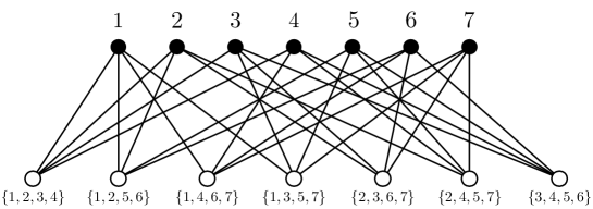
Figure 1. The incidence graph of $(7,4,2)$-design.

In view of Theorem 1.2, this graph satisfies the MNHD. Note that the graph above corresponds to the case (ii) in Proposition 2.1. We also exhibit below all regular bipartite graphs $X=(V,E)$ with $|V|\leq 30$ having four distinct Laplacian eigenvalues, according to van Dam–Spence [3, Appendix A].

$|V|$	$\sigma(L)$	$(v,k,\lambda)$
10	$\{0,3,5,8\}$	$(5,4,3)$
12	$\{0,4,6,10\}$	$(6,5,4)$
14	$\{0,5,7,12\}$	$(7,6,5)$
14	$\{0,3\pm\sqrt{2},6\}$	$(7,3,1)$
14	$\{0,4\pm\sqrt{2},8\}$	$(7,4,2)$
16	$\{0,6,8,14\}$	$(8,7,6)$
18	$\{0,7,9,16\}$	$(9,8,7)$
20	$\{0,8,10,18\}$	$(10,9,8)$
22	$\{0,9,11,20\}$	$(11,10,9)$
22	$\{0,5\pm\sqrt{3},10\}$	$(11,5,2)$

$|V|$	$\sigma(L)$	$(v,k,\lambda)$
22	$\{0,6\pm\sqrt{3},12\}$	$(11,6,3)$
24	$\{0,10,12,22\}$	$(12,11,10)$
26	$\{0,11,13,24\}$	$(13,12,11)$
26	$\{0,4\pm\sqrt{3},8\}$	$(13,4,1)$
26	$\{0,9\pm\sqrt{3},18\}$	$(13,9,6)$
28	$\{0,12,14,26\}$	$(14,13,12)$
30	$\{0,5,9,14\}$	$(15,7,3)$
30	$\{0,6,10,16\}$	$(15,8,4)$
30	$\{0,13,15,28\}$	$(15,14,13)$

On the other hand, we also find some examples of finite (not always regular) graphs with four Laplacian eigenvalues which are not bipartite but satisfy the MNHD.

Example 4.2 (regular, non-bipartite case).

Let $X$ be a finite 3-regular graph given by (a) in Fig. 2. The graph Laplacian of $X$ has four integral eigenvalues $0,2,3,5$. This means that the graph $X$ corresponds to the case (i) in Proposition 2.1. We can show that the graph $X$ actually satisfies the MNHD.

Proof.

The graph Laplacian $L$ of $X$ and its square $L^{2}$ are given by

$$L=\begin{pmatrix}3&-1&-1&0&0&-1\\ -1&3&0&-1&-1&0\\ -1&0&3&-1&0&-1\\ 0&-1&-1&3&-1&0\\ 0&-1&0&-1&3&-1\\ -1&0&-1&0&-1&3\\ \end{pmatrix},\qquad L^{2}=\begin{pmatrix}12&-6&-5&2&2&-5\\ -6&12&2&-5&-5&2\\ -5&2&12&-6&2&-5\\ 2&-5&-6&12&-5&2\\ 2&-5&2&-5&12&-6\\ -5&2&-5&2&-6&12\\ \end{pmatrix},$$

respectively. We decompose the set $(V\times V)\setminus\{(v_{i},v_{i})\,|\,i=1,2,\dots,6\}$ into $W_{1}\sqcup W_{2}\sqcup W_{3}$, where

$$W_{1} :=\{(v_{i},v_{j})\,|\,\text{$v_{i}$, $v_{j}$ are not adjacent}\},$$

$$W_{2} :=\{(v_{i},v_{j})\,|\,\text{$v_{i}$, $v_{j}$ are adjacent and $v_{i},v_{j},v_{k}$ form a triangle for some $k$}\},$$

$$W_{3} :=\{(v_{i},v_{j})\,|\,(v_{i},v_{j})\notin W_{1}\sqcup W_{2}\}.$$

Then the values of $\Delta_{k}=\Delta_{k}(v_{i},v_{j}),\,k=1,2,3$, and $\Delta_{k\ell}=\Delta_{k\ell}(v_{i},v_{j})$, $(k,\ell)=(1,2),(1,3),(2,3)$, are exhibited as follows:

	$\Delta_{1}$	$\Delta_{2}$	$\Delta_{3}$	$\Delta_{12}$	$\Delta_{13}$	$\Delta_{23}$
$(v_{i},v_{j})\in W_{1}$	$\frac{1}{3}$	$\frac{1}{2}$	$\frac{1}{6}$	$-\frac{1}{36}$	$-\frac{1}{12}$	$-\frac{1}{9}$
$(v_{i},v_{j})\in W_{2}$	$0$	$\frac{1}{2}$	$\frac{1}{2}$	$\frac{1}{12}$	$\frac{1}{12}$	$0$
$(v_{i},v_{j})\in W_{3}$	$\frac{1}{3}$	$0$	$\frac{2}{3}$	$-\frac{1}{9}$	$0$	$\frac{2}{9}$

As is seen, $\Delta_{k}(v_{i},v_{j})\geq 0,\,k=1,2,3$, holds in each case and we can follow the same argument as the proof of Theorem 1.2 to conclude that each function $h_{v_{i},v_{j}}(t)$ is monotonically non-decreasing in $[0,\infty)$. Therefore, we have shown that the graph $X$ satisfies the MNHD. ∎

Remark 4.3.

We should emphasize that the graph $X$ can be regarded as a Cayley graph of the symmetric group

$$\mathfrak{S}_{3}=\{v_{1}=e,\,v_{2}=\sigma,\,v_{3}=\tau,\,v_{4}=\sigma\tau,\,v_{5}=\tau\sigma,\,v_{6}=\sigma\tau\sigma\}$$

over the finite set $\{1,2,3\}$ with a generating set $\{\sigma,\tau,\tau^{2}\}$, where $e$ denotes the identity permutation and $\sigma=(1,2)$, $\tau=(1,2,3)$.

Example 4.4 (non-regular case).

Let $X$ be a 6-wheel graph, that is, a finite graph given by connecting a certain vertex to all vertices of a 5-cycle (see (b) in Fig. 2). The graph Laplacian of $X$ has four eigenvalues

$$\lambda_{0}=0,\qquad\lambda_{1}=\frac{7-\sqrt{5}}{2},\qquad\lambda_{2}=\frac{7+\sqrt{5}}{2},\qquad\lambda_{3}=6.$$

Although it is not regular, the graph $X$ also satisfies the MNHD.

Proof.

The graph Laplacian $L$ together with its square $L^{2}$ have on-diagonal components given by $L(v_{i},v_{i})=3,\,L^{2}(v_{i},v_{i})=12$ if $i=1,2,3,4,5$ and $L(v_{i},v_{i})=5,\,L^{2}(v_{i},v_{i})=30$ if $i=6$, and have off-diagonal ones given by

$$L(v_{i},v_{j}) =0, L^{2}(v_{i},v_{j}) =2, \text{if $v_{i}$ and $v_{j}$ are not adjacent},$$

$$L(v_{i},v_{j}) =-1, L^{2}(v_{i},v_{i}) =-5, \text{if $v_{i}$ and $v_{j}$ are adjacent with $i,j\neq 6$},$$

$$L(v_{i},v_{j}) =-1, L^{2}(v_{i},v_{j}) =-6, \text{otherwise}.$$

Then there are following four possibilities for the pair $(i,j)$:

1. $i,j=1,2,3,4,5$ and $v_{i},v_{j}$ are not adjacent,

2. $i,j=1,2,3,4,5$ and $v_{i},v_{j}$ are adjacent,

3. $i=1,2,3,4,5$ and $j=6$,

4. $i=6$ and $j=1,2,3,4,5$.

The values of $\Delta_{k}=\Delta_{k}(v_{i},v_{j}),\,k=1,2,3$, and $\Delta_{k\ell}=\Delta_{k\ell}(v_{i},v_{j})$, $(k,\ell)=(1,2),(1,3),(2,3)$, are listed as follows:

	$\Delta_{1}$	$\Delta_{2}$	$\Delta_{3}$	$\Delta_{12}$	$\Delta_{13}$	$\Delta_{23}$
(i)	$\frac{\sqrt{5}+5}{10}$	$\frac{5-\sqrt{5}}{10}$	0	$-\frac{2\sqrt{5}}{25}$	$-\frac{\sqrt{5}+5}{300}$	$-\frac{5-\sqrt{5}}{300}$
(ii)	$\frac{5-\sqrt{5}}{10}$	$\frac{\sqrt{5}+5}{10}$	0	$\frac{2\sqrt{5}}{25}$	$-\frac{5-\sqrt{5}}{300}$	$-\frac{\sqrt{5}+5}{10}$
(iii)	$\frac{2}{5}$	$\frac{2}{5}$	$\frac{1}{5}$	0	$\frac{1}{15}$	$\frac{1}{15}$
(iv)	0	0	1	0	0	0

We observe that $\Delta_{k}(v_{i},v_{j})\geq 0,\,k=1,2,3$, holds in each case. Therefore, by following the same argument as the proof of Theorem 1.2, we conclude that the function $h_{v_{i},v_{j}}(t)$ is monotonically non-decreasing in $[0,\infty)$, which implies that the graph $X$ does satisfies the MNHD. ∎

Figure 2. Finite graphs with four Laplacian eigenvalues.

In the present paper, we have proved that every finite, regular and bipartite graph with four distinct Laplacian eigenvalues satisfies the MNHD. However, in view of Examples 4.2 and 4.4, our results may be extended to more general cases such as at least non-bipartite cases. Indeed, we expect that the MNHD truly holds for all finite regular graphs with four Laplacian eigenvalues, which is left as an interesting open problem. Simultaneously, it is also interesting to investigate the cases of non-regular graphs.

Recall that every finite abelian Cayley graph satisfies the MNHD, which was shown in Price [8]. It is known that the symmetric group $\mathfrak{S}_{3}$ is a typical example of finite groups which are not abelian but solvable. As we mentioned in Example 4.2 and Remark 4.3, the Cayley graph of $\mathfrak{S}_{3}$ enjoys the MNHD. On the other hand, the finite lamplighter group, which is also known as an example of finite solvable groups, does not satisfy the MNHD (see Regev–Shinkar [9]). By taking these circumstances into account, one may ask what kinds of finite non-commutative groups satisfy the MNHD. In particular, we left the following as an open problem. Does every finite nilpotent Cayley graph satisfy the MNHD?

Acknowledgements: The second-named author would like to thank Professor Ryokichi Tanaka for informing him of the results in Regev–Shinkar [9] and Price [8] when he visited Tohoku University in June 2017, and for giving him valuable comments. This work is supported by JSPS KAKENHI Grant Number 19K23410.

References

• [1] A. E. Brouwer and W. H. Haemers: Spectra of Graphs, Universitext, Springer, New York, 2012.
• [2] E. R. van Dam: Regular graphs with four eigenvalues, Linear Algebra Appl. 226, 228 (1995), 139–162.
• [3] E. R. van Dam and E. Spence: Small regular graphs with four eigenvalues, Discrete Math. 189 (1998), 233–257.
• [4] X. Huang and Q. Huang: On regular graphs with four distinct eigenvalues, Linear Algebra Appl. 512 (2017), 219–233.
• [5] X. Huang and Q. Huang: On graphs with three or four distinct normalized Laplacian eigenvalues, Algebra Colloq. 26 (2019), 65–82.
• [6] A. Mohammadian and B.  Tayfeh-Rezaie: Graphs with four distinct Laplacian eigenvalues, J. Algebraic Combin. 34 (2011), 671–682.
• [7] B. Nica: A note on normalised heat diffusion for graphs, Bull. Aust. Math. Soc. 102 (2020), 1–6.
• [8] T. M. Price: An inequality for the heat kernel on an Abelian Cayley graph, Electron. Commun. Probab. 22 (2017), 8 pages.
• [9] O. Regev and I. Shinkar: A counterexample to monotonicity of relative mass in random walks, Electron. Commun. Probab. 21 (2016), 8 pages.