Geometric Manipulation of a Decoherence-Free Subspace in Atomic Ensembles

Abstract

We consider an ensemble of atoms with $\Lambda$-type level structure trapped in a single-mode cavity, and propose a geometric scheme of coherent manipulation of quantum states on the subspace of zero-energy states within the quantum Zeno subspace of the system. We find that the particular subspace inherits the decoherence-free nature of the quantum Zeno subspace and features a symmetry-protected degeneracy, fulfilling all the conditions for a universal scheme of arbitrary unitary operations on it.

Coherent manipulation of quantum states is an essential part of various quantum technologies ranging from quantum-enhanced precision measurement to more ambitious goals, like quantum simulation and quantum information processing. While there remain considerable challenges to achieve reliable quantum-state engineering on large scales [1], a number of schemes to suppress and/or control decoherence and improve operational imperfections have been proposed and are currently under investigation. Notable examples include approaches based on decoherence-free subspaces [2, 3, 4], dynamical decoupling [5, 6, 7], quantum error correction [8, 9, 10], and holonomic manipulation [11, 12, 13, 14, 15, 16, 17, 18, 19, 20]. In addition, topological approaches [21, 22, 23] have recently attracted remarkable interest, due to the highly appealing prospect of topologically protected operations. However, physical systems with robust and easily addressable topological entities are yet to be discovered or developed [24, 25, 26, 27, 28].

In this work, we combine the self-correcting features of geometric methods and the concept of decoherence-free subspaces. More specifically, we develop a holonomic manipulation scheme based on ensembles of atoms with $\Lambda$-type level structure, trapped in a single-mode cavity [29]. To implement universal holonomies, a crucial requirement is the degeneracy of the operational subspace (or, the equally-demanding cyclic-evolution condition [30, 14]). Here we identify a generally degenerate subspace, whose decoherence-free feature is inherited from the quantum Zeno subspace [31]. The atomic systems considered here have been popular for studies of dissipation-based quantum computation [3], quantum gates based on adiabatic passages (or shortcuts to them) [32, 33], non-Adiabatic holonomic quantum computation [34], and generation of highly entangled states [35, 36, 37, 38]. However, the degeneracy allowing for holonomic manipulation, not to speak of the combination with the decoherence-free character of the quantum Zeno subspace, has not been exploited in those works. By focusing on the simplest realization of our scheme, we prove the universality of the holonomic gates. Combining the self-correcting character of unitary operations implemented through geometric methods with the decoherence-free feature of this particular subspace might effectively provide a high level of fault tolerance, practically comparable to topological methods.

Degenerate Decoherence-Free Subspace.

We consider $n$ identical atoms with $\Lambda$-type level structure [29] inside a single-mode cavity (see Fig. 1). The two ground states of each atom are denoted by $\mathinner{\lvert{\textstyle 0}\rangle}$ and $\mathinner{\lvert{\textstyle 1}\rangle}$, respectively, and the excited state by $\mathinner{\lvert{\textstyle 2}\rangle}$. The transition $\mathinner{\lvert{\textstyle 0}\rangle}\leftrightarrow\mathinner{\lvert{\textstyle 2}\rangle}$ is induced by the cavity photon while the transition $\mathinner{\lvert{\textstyle 1}\rangle}\leftrightarrow\mathinner{\lvert{\textstyle 2}\rangle}$ is driven resonantly by an external classical field. All atoms are assumed to be coupled to the cavity photon with a uniform strength $g$. We divide the atoms into two subensembles, $A$ containing $p$ atoms and $B$ with the rest, and separately tune their characteristic Rabi transition amplitudes, $\Omega_{a}$ and $\Omega_{b}$, respectively (atoms in each subensemble have a uniform Rabi transition amplitude). In the interaction picture, the dynamics of the system is governed by the Hamiltonian $\hat{H}=\hat{H}_{g}+\hat{H}_{\Omega}$ with

$$\hat{H}_{g}= g\sum_{j=1}^{n}\hat{c}|2\rangle_{j}\langle 0|+\mathrm{H.c.}\,,$$ (1a)

$$\hat{H}_{\Omega}= \Omega_{a}\sum_{j=1}^{p}|2\rangle_{j}\langle 1|+\Omega_{b}\sum_{j=p+1}^{n}|2\rangle_{j}\langle 1|+\mathrm{H.c.}\,,$$ (1b)

where $\hat{c}$ is the annihilation operator of the cavity photon and $\mathinner{\lvert{\textstyle s}\rangle}_{j}$ denotes the $j$th atom in state $\mathinner{\lvert{\textstyle s}\rangle}$ ($s=0,1,2$).

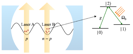
Figure 1: Schematics of the atomic ensembles in a single-mode cavity (left), and the level structure of each atom (right).

To identify the relevant decoherence-free subspace, we exploit the symmetries in the Hamiltonian (1): First, the total excitation number $\hat{N}=\hat{c}^{\dagger}\hat{c}+\sum_{j}(|1\rangle_{j}\langle 1|+|2\rangle_{j}\langle 2|)$ is conserved, $[\hat{N},\hat{H}]=0$. It allows us to focus on an invariant subspace $\mathcal{H}_{N}$ with a particular excitation number $N$. Throughout this work, the excitation number is assumed equal to the number $p$ of atoms in subensemble $A$, which simplifies the initial preparation of the system. Second, the Hamiltonian is invariant under exchange of any pair of atoms within each subensemble. Among various invariant subspaces, we are mainly interested in the subspace $\mathcal{S}^{A}\otimes\mathcal{S}^{B}\subset\mathcal{H}_{p}$ of states which are totally symmetric in each subensemble. Within $\mathcal{S}_{A}$ or $\mathcal{S}_{B}$, the atoms behave like bosons. We describe the atoms in subensemble $A$ by the bosonic operators $\hat{a}_{s}$ associated with the atomic levels $\mathinner{\lvert{\textstyle s}\rangle}$. The atoms in $B$ are described by similar operators $\hat{b}_{s}$. Expressed in terms of these bosonic operators, the Hamiltonian terms in Eq. (1) read as

$$\hat{H}_{g} =g\left(\hat{a}_{2}^{\dagger}\hat{a}_{0}+\hat{b}_{2}^{\dagger}\hat{b}_{0}\right)\hat{c}+\mathrm{H.c.}$$ (2a)

$$\hat{H}_{\Omega} =\Omega_{a}\hat{a}_{2}^{\dagger}\hat{a}_{1}+\Omega_{b}\hat{b}_{2}^{\dagger}\hat{b}_{1}+\mathrm{H.c.}$$ (2b)

Likewise, we rewrite the conservation of the total excitation number as $\sum_{s=1}^{2}\hat{a}_{s}^{\dagger}\hat{a}_{s}+\sum_{s=1}^{2}\hat{b}_{s}^{\dagger}\hat{b}_{s}+\hat{c}^{\dagger}\hat{c}=p$, and the constraints of having a fixed number of atoms in each subensemble as $\sum_{s=0}^{2}\hat{a}_{s}^{\dagger}\hat{a}_{s}=p$ and $\sum_{s=0}^{2}\hat{b}_{s}^{\dagger}\hat{b}_{s}=n-p$.

Third, and most importantly, we bring into play the total occupation number in the excited level $\hat{N}_{2}=\hat{a}_{2}^{\dagger}\hat{a}_{2}+\hat{b}_{2}^{\dagger}\hat{b}_{2}$, with its associated even-odd parity operator:

$$\hat{\Pi}_{2}:=\exp(i\pi\hat{N}_{2}),$$ (3)

which carries an interesting “anti-symmetry” [39]:

$$\{\hat{\Pi}_{2},\hat{H}\}=0.$$ (4)

This property follows from the fact that any atomic transition occurs through the excited level $\mathinner{\lvert{\textstyle 2}\rangle}$. The anti-symmetry implies that, in the parity basis, the Hamiltonian is block-off-diagonal, and leads to one of our main findings: the zero-energy subspace of $\mathcal{S}_{A}\otimes\mathcal{S}_{B}$ is always degenerate as long as $p>1$. We refer to the Supplemental Material [40] for the details of the general proof.

Within $\mathcal{S}_{A}\otimes\mathcal{S}_{B}$, we identify a zero-energy subspace which is decoherence-free by considering the limit of quantum Zeno dynamics ($g\to\infty$). Under this condition, photon lekeage out of the cavity is completely suppressed within the subspace $\mathcal{Z}\subset\mathcal{S}_{A}\otimes\mathcal{S}_{B}$ of zero-photon states, a so-called quantum Zeno subspace [31]. Since the coupling of atoms with the electromagnetic field is mainly to the discrete mode of the cavity, spontaneous decay from state $|2\rangle$ is also strongly suppressed [41, 3, 31], and $\cal Z$ can be considered as a decoherence-free subspace. Within $\cal Z$, $H_{g}=0$, and the Hamiltonian $\hat{H}$ $(=\hat{H}_{\Omega})$ still bears the anti-symmetry Eq. (4), hence the zero-energy subspace $\cal D$ embedded in the Zeno subspace, $\cal D\subset\cal Z$, is always degenerate for $p>1$. Besides being robust against photon decay, the states in $\mathcal{D}$ are dynamically irresponsive to the external driving fields, as $\hat{H}_{\Omega}=0$ within $\mathcal{D}$. We call them “dark states” to distinguish them from other zero-energy states outside $\mathcal{Z}$.

In short, the subspace $\mathcal{D}$ of dark states is our desired decoherence-free subspace. Since the dark states are dynamically irresponsive, below we propose to manipulate them by geometric means, that is, using non-Abelian geometric phases (holonomies). $\mathcal{D}$ is separated by a finite energy gap $(\sim\Omega_{a/b})$ from the rest of the spectrum within $\mathcal{Z}$, hence is stable in quasi-adiabatic processes.

To be specific, from now on we will focus on the case of four atoms ($n=4$) and two excitations ($p=2$). Then, the quantum Zeno subspace $\mathcal{Z}$ consists of the following 6 basis states (excluding a state which is completely decoupled from the rest):

$$\mathinner{\lvert{\textstyle\zeta_{1}}\rangle} =\mathinner{\lvert{\textstyle 0020,0}\rangle},\;\;\mathinner{\lvert{\textstyle\zeta_{2}}\rangle}=\mathinner{\lvert{\textstyle 1010,0}\rangle},\;\;\mathinner{\lvert{\textstyle\zeta_{3}}\rangle}=\mathinner{\lvert{\textstyle 2000,0}\rangle},$$

$$\mathinner{\lvert{\textstyle\zeta_{4}}\rangle} =\frac{\mathinner{\lvert{\textstyle 0002,0}\rangle}-\mathinner{\lvert{\textstyle 0101,0}\rangle}+\mathinner{\lvert{\textstyle 0200,0}\rangle}}{\sqrt{3}},$$

$$\mathinner{\lvert{\textstyle\zeta_{5}}\rangle} =\frac{\mathinner{\lvert{\textstyle 0110,0}\rangle}-\sqrt{2}\mathinner{\lvert{\textstyle 0011,0}\rangle}}{\sqrt{3}},$$

$$\mathinner{\lvert{\textstyle\zeta_{6}}\rangle} =\frac{\mathinner{\lvert{\textstyle 1001,0}\rangle}-\sqrt{2}\mathinner{\lvert{\textstyle 1100,0}\rangle}}{\sqrt{3}},$$ (5)

where $\mathinner{\lvert{\textstyle n_{a_{1}}n_{a_{2}}n_{b_{1}}n_{b_{2}},n_{c}}\rangle}$ indicate the boson numbers. Note that we have not specified the bosonic occupations of state $|0\rangle$, as they are fixed by the constraints $n_{a_{0}}=p-n_{a_{1}}-n_{a_{2}}$ and $n_{b_{0}}=n-p-n_{b_{1}}-n_{b_{2}}$. Within $\mathcal{Z}$, the matrix representation of the Hamiltonian in the specified basis is given by

$$\hat{H}\doteq\begin{pmatrix}0&D^{\dagger}\\ D&0\end{pmatrix}$$ (6)

with the off-diagonal subblock

$$D=\begin{pmatrix}-\frac{2\Omega_{b}}{\sqrt{3}}&\frac{\Omega_{a}}{\sqrt{3}}&0&-\Omega_{b}^{*}\\ 0&\frac{\Omega_{b}}{\sqrt{3}}&-\frac{2\Omega_{a}}{\sqrt{3}}&-\Omega_{a}^{*}\end{pmatrix}.$$ (7)

It is clear that the dark-states subspace $\mathcal{D}$ is nothing but the null space of $D$, hence is two-fold degenerate, in agreement with our general findings. Indeed, we find the following (unnormalized) basis states spanning $\mathcal{D}$

$$\mathinner{\lvert{\textstyle D_{1}}\rangle}=\mathinner{\lvert{\textstyle\zeta_{1}}\rangle}\Omega_{a}^{2}+\mathinner{\lvert{\textstyle\zeta_{2}}\rangle}2\Omega_{a}\Omega_{b}+\mathinner{\lvert{\textstyle\zeta_{3}}\rangle}\Omega_{b}^{2}$$ (8)

and

$$\mathinner{\lvert{\textstyle D_{2}}\rangle}= \mathinner{\lvert{\textstyle\zeta_{1}}\rangle}\sqrt{3}(\Omega_{b}^{*})^{2}\left(3|\Omega_{a}|^{2}+|\Omega_{b}|^{2}\right)$$

$${}-\mathinner{\lvert{\textstyle\zeta_{2}}\rangle}2\sqrt{3}\Omega_{a}^{*}\Omega_{b}^{*}\left(|\Omega_{a}|^{2}+|\Omega_{b}|^{2}\right)$$

$${}+\mathinner{\lvert{\textstyle\zeta_{3}}\rangle}\sqrt{3}(\Omega_{a}^{*})^{2}\left(|\Omega_{a}|^{2}+3|\Omega_{b}|^{2}\right)$$

$${}-\mathinner{\lvert{\textstyle\zeta_{4}}\rangle}2\left(|\Omega_{a}|^{4}+4|\Omega_{a}\Omega_{b}|^{2}+|\Omega_{b}|^{4}\right)\,.$$ (9)

Holonomic Manipulation.

With a time-dependent Hamiltonian, the quantum state acquires not only dynamical phases but also purely geometric phases, either Abelian [42] or non-Abelian [43]. Suppose that the Hamiltonian $\hat{H}(t)=\hat{H}(R_{\mu}(t))$ depending on slowly varying control parameters $R_{\mu}(t)\in\mathbb{C}$ ($\mu=1,2,\dots$) maintains a degenerate subspace of eigenstates $\mathinner{\lvert{\textstyle\eta_{j}(R_{\mu}(t))}\rangle}$ ($j=1,2,\dots$) at any instant $t$ of time. The adiabatic evolution of the states in the subspace is governed by the unitary operator (up to a global phase factor)

$$\hat{U}(t,t^{\prime})=\sum_{ij}|\eta_{i}(R_{\mu}(t))\rangle U_{ij}(t,t^{\prime})\mathinner{\langle{\textstyle\eta_{j}(R_{\mu}(t^{\prime}))}\rvert}.$$ (10)

The adiabatic-evolution operator $\hat{U}$ depends only on the path $\mathcal{C}$ in parameter space [43], and the corresponding unitary matrix $U$ is given by

$$U(\mathcal{C})=\mathcal{P}\exp\left(-\int_{\mathcal{C}}A^{\mu}dR_{\mu}\right)\,,$$ (11)

where $\mathcal{P}$ denotes the path ordering and the matrix

$$A_{ij}^{\mu}=\langle\eta_{i}(R_{\mu})|\frac{\partial}{\partial R_{\mu}}|\eta_{j}(R_{\mu})\rangle$$ (12)

is the non-Abelian gauge potential describing the connection between the instantaneous bases at different points in parameter space. We will denote the non-Abelian holonomy interchangeably either by the operator $\hat{U}(\mathcal{C})$ or the matrix $U(\mathcal{C})$.

In our case, control parameters are the complex Rabi transition amplitudes, $\Omega_{a}=\Omega\sin\theta\,e^{i\phi_{a}}$ and $\Omega_{b}=\Omega\cos\theta\,e^{i\phi_{b}}$, and we modulate $\theta$ and $\phi_{\mu}$ ($\mu=a,b$) in time. For most physical applications, $\theta=\pi/4$ ($|\Omega_{a}|=|\Omega_{b}|$) is the most interesting configuration, and many adiabatic paths either (or both) start from or end up with $\theta=\pi/4$. We find it convenient to split the path $\mathcal{C}$ into segments $\mathcal{C}=\mathcal{C}_{\theta}+\mathcal{C}_{\phi}+\mathcal{C}_{\theta}^{\prime}+\mathcal{C}_{\phi}^{\prime}+\dots\,.$ In the amplitude-modulation segments $\mathcal{C}_{\theta}(\theta_{2},\theta_{1})$, only $\theta$ is varied from $\theta_{1}$ to $\theta_{2}$ keeping $\phi_{\mu}=0$. In the phase-modulation segments $\mathcal{C}_{\phi}(m_{a},m_{b};\theta)$, only $\phi_{\mu}$ are modulated from 0 to $2\pi{m_{\mu}}$ ($m_{\mu}\in\mathbb{Z}$) with $\theta$ fixed.

The effects of amplitude and phase modulation are complementary: For $\mathcal{C}_{\theta}(\theta_{1},\theta_{0})$, the non-Abelian holonomy is given by [40]

$$U(\mathcal{C}_{\theta}(\theta_{1},\theta_{0}))=\exp\left\{-i\left[c_{y}(\theta_{1})-c_{y}(\theta_{0})\right]\sigma_{y}\right\},$$ (13)

with $c_{y}(\theta)=-\arctan\sqrt{(19-5\cos 4\theta)/6}\,,$ where $\sigma^{\mu}$ are the Pauli matrices in the basis of (8) and (Degenerate Decoherence-Free Subspace.). $U(\mathcal{C}_{\theta})$ thus describes a rotation around the fixed $y$-axis, with only the angle depending on $\mathcal{C}_{\theta}$. On the other hand, $\mathcal{C}_{\phi}(m_{a},m_{b};\theta)$ gives rise to [40]

$$U(\mathcal{C}_{\phi})=\exp[ic_{x}\sigma_{x}+ic_{z}\sigma_{z}]$$ (14)

with the coefficients

$$c_{x}= \frac{2\sqrt{6}(m_{a}-m_{b})\pi\sin 2\theta\sin 4\theta}{(5-\cos 4\theta)\sqrt{19-5\cos 4\theta)}},$$

$$c_{z}= \frac{(m_{a}+m_{b})\pi(\cos 8\theta-20\cos 4\theta+51)}{(5-\cos 4\theta)(5\cos 4\theta-19)}$$

$$-\frac{(m_{a}-m_{b})\pi(16\cos 6\theta-96\cos 2\theta)}{(5-\cos 4\theta)(5\cos 4\theta-19)}\,.$$ (15)

$U(\mathcal{C}_{\phi})$ corresponds to a rotation around an axis in the $xz$-plane with both axis and angle depending on $\mathcal{C}_{\phi}$.

Universality.

Now we address the following question: Is it possible to implement an arbitrary unitary transformation by combining $\hat{U}(\mathcal{C}_{\phi})$ and $\hat{U}(\mathcal{C}_{\theta})$? This is a non-trivial question, as the rotation axes and angles of $\hat{U}(\mathcal{C}_{\phi})$ and $\hat{U}(\mathcal{C}_{\theta})$ of our concern are not continuous. However, we should recall that any two-dimensional unitary transformation can be realized to arbitrary accuracy by combining two rotations around different axes, if their angles are irrational multiples of $2\pi$. Therefore, given a desired accuracy, we can implement any unitary transformation within $\mathcal{D}$ by combining $\hat{U}(\mathcal{C}_{\phi})$ and $\hat{U}(\mathcal{C}_{\theta})$. Alternatively, Fig. 2 demonstrates that two different choices of $\hat{U}(\mathcal{C}_{\phi})$ are already sufficient. We have constructed random sequences of $\hat{U}_{1}$ and $\hat{U}_{2}$ of varying lengths, with $\hat{U}_{1}=\hat{U}(\mathcal{C}_{\phi}(1,0;\pi/6))$ and $\hat{U}_{2}=\hat{U}(\mathcal{C}_{\phi}(0,-1;\pi/6))$, and applied them on $\mathinner{\lvert{\textstyle D_{1}}\rangle}$. Each point in Fig. 2 represents the resulting quantum state. As seen, the states densely fill up the Bloch sphere.

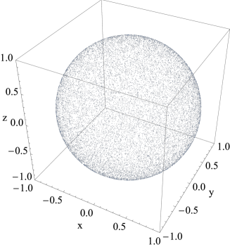
Figure 2: Bloch sphere densely filled with states resulting from random sequences of two holonomies $\hat{U}_{1}$ and $\hat{U}_{2}$, applied to $\mathinner{\lvert{\textstyle D_{1}}\rangle}$. We have chosen $\hat{U}_{1}=\hat{U}(\mathcal{C}_{\phi}(1,0;\pi/6))$ and $\hat{U}_{2}=\hat{U}(\mathcal{C}_{\phi}(0,-1;\pi/6))$.

For the purpose of demonstration, we further provide explicit adiabatic paths that generate the elementary Pauli $X$ and $Z$. We consider the sequence:

$$\hat{W}(m_{a},m_{b};\theta_{1}):=\\ {}\hat{U}(\mathcal{C}_{\theta}(\pi/4,\theta_{1}))\hat{U}(\mathcal{C}_{\phi}(m_{a},m_{b};\theta_{1}))\hat{U}(\mathcal{C}_{\theta}(\theta_{1},\pi/4)).$$ (16)

Pauli $Z$ is extremely simple to implement, as it is identical to $\hat{W}(1,0;\pi/4)$.

While Pauli $X$ cannot be implemented exactly, the following procedure enables an approximate implementation to arbitrary accuracy: First recall from Eq. (13) that $\hat{U}(\mathcal{C}_{\theta}(\pi/4,\theta_{1}))=\hat{U}^{\dagger}(\mathcal{C}_{\theta}(\theta_{1},\pi/4))$ is a rotation around the $y$-axis. Therefore, just like $U(\mathcal{C}_{\phi})$, $\hat{W}$ is a rotation around an axis that is still in the $xz$-plane [see Eq. (14)]. One can numerically find a value $\theta_{1}^{*}$ such that $\hat{W}(m_{a},m_{b};\theta_{1}^{*})$ is a rotation along the $x$-axis. The rotation angle is an irrational multiple of $2\pi$, thus $\hat{W}(m_{a},m_{b};\theta_{1}^{*})$ does not yet realize the Pauli $X$. However, repeated applications of $\hat{W}(m_{a},m_{b};\theta_{1}^{*})$ can reach any desired angle, say $\pi$, with arbitrary accuracy. This is illustrated with $m_{a}=0$ and $m_{b}=1$ in Fig. S1 of the Supplemental Material [40].

Application.

As an example of application of our scheme, we consider the generation of symmetric Dicke states (unnormalized)

$$\mathinner{\lvert{\textstyle\Phi_{n}^{p}}\rangle}=\sum_{i}\mathcal{P}_{i}\mathinner{\lvert{\textstyle 1}\rangle}^{\otimes p}\otimes\mathinner{\lvert{\textstyle 0}\rangle}^{\otimes(n-p)}$$ (17)

with directional “angular momentum” $(n/2-p)$, where $\sum_{i}\mathcal{P}_{i}\cdots$ denotes the sum over distinct permutations of all $n$ atoms. Due to their rich entanglement [44, 45], Dicke states have attracted considerable interest as valuable resources, e.g., for precision measurement [46, 47, 48].

We first note that, regardless of parameters, there always exists a special dark state which is immune to spontaneous decay from level $|2\rangle$ (unnormalized):

$$\mathinner{\lvert{\textstyle E_{n}^{p}}\rangle}=\left[\Omega_{a}\hat{a}_{0}^{\dagger}-g\hat{c}\hat{a}_{1}^{\dagger}\right]^{p}\left[\Omega_{b}\hat{b}_{0}^{\dagger}-g\hat{c}\hat{b}_{1}^{\dagger}\right]^{n-p}(\hat{c}^{\dagger})^{p}\mathinner{\lvert{\textstyle\phantom{.}}\rangle},$$ (18)

where $\mathinner{\lvert{\textstyle\phantom{.}}\rangle}$ denotes the vacuum state (no particle at all). A key observation is that, when $\Omega_{a}=\Omega_{b}$, $\mathinner{\lvert{\textstyle E_{n}^{p}}\rangle}$ is identical to the symmetric Dicke state $\mathinner{\lvert{\textstyle\Phi_{n}^{p}}\rangle}$ in the quantum Zeno limit. More specifically, considering the example of $n=4$ and $p=2$, $\mathinner{\lvert{\textstyle E_{n}^{p}}\rangle}$ reads as (unnormalized)

$$\mathinner{\lvert{\textstyle E_{4}^{2}}\rangle}=|2000,0\rangle+2|1010,0\rangle+|0020,0\rangle$$ (19)

in the bosonic notations or, equivalently:

$$\mathinner{\lvert{\textstyle E_{4}^{2}}\rangle} =|1\rangle_{1}|1\rangle_{2}|0\rangle_{3}|0\rangle_{4}+|1\rangle_{1}|0\rangle_{2}|1\rangle_{3}|0\rangle_{4}$$

$$+|1\rangle_{1}|0\rangle_{2}|0\rangle_{3}|1\rangle_{4}+|0\rangle_{1}|1\rangle_{2}|1\rangle_{3}|0\rangle_{4}$$

$$+|0\rangle_{1}|1\rangle_{2}|0\rangle_{3}|1\rangle_{4}+|0\rangle_{1}|0\rangle_{2}|1\rangle_{3}|1\rangle_{4}$$ (20)

in the traditional representation.

We want to generate the dark state in (Application.) [or equivalently (19)] starting from a product state $|1\rangle_{1}|1\rangle_{2}|0\rangle_{3}|0\rangle_{4}$. Note that both the initial product state and the desired dark state in (Application.) belong to $\mathcal{D}$. The former for $\Omega_{a}=0$ and $\Omega_{b}=\Omega$ and the latter for $\Omega_{a}=\Omega_{b}=\Omega/\sqrt{2}$. That is, the two states are adiabatically connected and can be transformed into each other by the non-Abelian holonomy discussed above. To this end, we slightly modify the sequence in (16) to

$$\hat{W}^{\prime}(m_{a},m_{b};\theta_{1}):=\\ \hat{U}(\mathcal{C}_{\theta}(\pi/4,\theta_{1}))\hat{U}(\mathcal{C}_{\phi}(m_{a},m_{b};\theta_{1}))\hat{U}(\mathcal{C}_{\theta}(\theta_{1},0))\,.$$ (21)

In this sequence, $\theta$ starts from 0 and moves to $\theta_{1}$, then $\phi_{\mu}$ make round trips from $0$ to integer multiples of $2\pi$, keeping $\theta=\theta_{1}$, and finally $\theta$ moves from $\theta_{1}$ to $\pi/4$, where the Hamiltonian becomes symmetric between subensembles $A$ and $B$. We find that the adiabatic paths specified by the parameters $\{m_{a},m_{b}\}=\{-24,1\}$, and $\theta_{1}=0.669$ in the sequence (21) brings the initial product state to the symmetric Dicke state in (Application.) with fidelity close to 1.

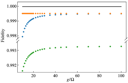
Figure 3: Fidelity as a function of $g$ between the desired Dicke state and the state from the adiabatic evolution $\hat{W}^{\prime}(-24,1;0.669)$ (black solid line). We also compute the fidelity by numerically solving the Schrödinger equation along the path $\mathcal{C}_{\theta}(\pi/4,\theta_{1})+\mathcal{C}_{\phi}(-24,1;\theta_{1})+\mathcal{C}_{\theta}(\theta_{1},0)$ within $\mathcal{Z}$ (orange dots) and in the whole $\mathcal{S}_{A}\otimes\mathcal{S}_{B}$ (blue dots), where $\theta_{1}=0.669$. For comparison, the fidelity of the state from the simulation along the path $\mathcal{C}_{\theta}(\pi/4,0)$ is also shown with green dots. The discrepancy between the orange dots and the black line is due to the finite simulation time, $T=8000/g$. black

We also performed a time-dependent simulation with finite ramping time of the parameters, by numerically solving the Schrödinger equation in the whole space $\mathcal{S}_{A}\otimes\mathcal{S}_{B}$ (not restricted to $\mathcal{D}$ or $\mathcal{Z}$). As shown in Fig. 3, the simulation results agree very well with the holonomic treatment, as long as $g/\Omega>10$. This implies that, protected by a finite energy gap in the spectrum, our holonomic method in the adiabatic limit can be performed at realistic speeds.

We remark that it was previously proposed to achieve the same goal solely based on the quantum Zeno dynamics [36], which effectively corresponds to skipping the phase modulation sequence $\mathcal{C}_{\phi}$ in Eq. (21). This approach also assumes a finite detuning in the classical driving fields, which lifts the degeneracy in $\mathcal{D}$ and suppresses unwanted transitions to other states. In the absence of detuning, however, transitions within $\mathcal{D}$ degrade the fidelity of the final state with the desired target state. The comparison in Fig. 3 shows that the phase modulation path $\mathcal{C}_{\phi}$ plays a significant role to readjust the state to the desired target state.

In conclusion, we have considered a system of atoms with $\Lambda$-type level structure trapped in a single-mode cavity, and proposed a geometric scheme of coherent manipulation on the subspace of zero-energy states within the quantum Zeno subspace. These states inherit the decoherence-free nature of the quantum Zeno subspace and feature a symmetry-protected generic degeneracy, fulfilling all the conditions for a universal scheme of arbitrary unitary operations on it. Here we have taken a specific example with $n=4$ and $p=2$ for the purpose of demonstration of the main idea. In principle, this method can be extended to an arbitrary number of atoms and excitations.