Enhanced dissipation, hypoellipticity for passive scalar equations with fractional dissipation
Siming He
Abstract.
We consider the passive scalar equations subject to shear flow advection and fractional dissipation. The enhanced dissipation estimates are derived. For the classical passive scalar equation (), our result agrees with the sharp one obtained in [46].
simhe@math.duke.edu, Department of Mathematics, Duke University
Acknowledgment. This work was supported in part by NSF grants DMS 2006660, DMS grant 2006372. The author would like to thank Alexander Kiselev for many discussions. The author would also like to thank the referees for pointing out important generalizations of the main result.
1. Introduction
We consider the passive scalar equations subject to shear advection and fractional dissipation:
(1.1)
(1.2)
Their hypoelliptic counterparts read as follows
(1.3)
(1.4)
Here denote the densities transported by the flow. The fractional dissipation order takes value in . The viscosity is small, i.e., . Since the dynamics (1.1), (1.3) preserve the average of solutions, one can subtract the average and assume without loss of generality that ([18])
(1.5)
Assume the shear flow profiles have finitely many critical points . The vanishing order associated with each critical point is defined as the smallest integer such that
(1.6)
The maximal vanishing order of the shear flow profile is . Since any smooth shear flow profiles on the torus have at least one critical point, the maximal vanishing orders are greater than . If the maximal vanishing order is , the shear flow is nondegenerate.
The enhanced dissipation effect of the classical passive scalar equations () subject to shear flow has attracted much attentions from the mathematical fluid mechanics community in the recent years. In the paper [6], J. Bedrossian and M. Coti-Zelati applied hypocoercivity functional ([44, 3]) to show that if is smaller than a universal threshold , the following enhanced dissipation estimate holds for some universal constants ,
(1.7)
Their result was later improved by D. Wei [46]. Combining the resolvent estimates and a Gearhart-Prüss type theorem, D. Wei removed the logarithmic correction in the dissipation rate. Later, M. Coti Zelati and T. Drivas showed that the enhanced dissipation rate appeared in (1.7) is sharp ([20]).
The underlying mechanism of the enhanced dissipation effect is that the shear flow advection triggers the phase mixing phenomenon ([39, 49, 12]), which amplifies the damping effect of the dissipation operators (see, e.g., [14, 18]). Similar phase mixing phenomena play a fundamental role in Landau damping, see, e.g., [39, 13, 5]. Enhanced dissipation effect of the rough shear flows, and its relation to mixing are explored in [46, 16].
The shear flows’ enhanced dissipation effect has found applications in various problems in fluid mechanics, plasma physics, and biology. First of all, the shear flows’ enhanced dissipation is one of the stabilizing mechanisms in hydrodynamic stability. We refer the interested readers to the study of stability of the Couette flows ([41, 14, 9, 7, 8, 15, 10]), the Poiseuille flows ([21, 22]), and the Kolmogorov flows ([47, 30, 37]). In plasma physics, the enhanced collision effect, equivalent to the enhanced dissipation effect, stabilizes the plasma and prevents the echo-chain instability ([4]). In biology, the enhanced dissipation effect of the ambient shear flows suppresses the chemotactic blow-ups ([11, 27]).
The enhanced dissipation effect of the shear flow is heterogeneous. If the initial data of the passive scalar equation depends only on -variables, solves the heat equation, and no enhanced dissipation is possible. Hence the zero-average constraint (1.5) is enforced. However, there exist fluid flows inducing the enhanced dissipation effect in all directions. These are the relaxation-enhancing flows. The concept is first introduced by P. Constantin et al., [17]. In the papers [18, 25], the authors prove that flows with mixing properties are relaxation enhancing. Explicit constructions of mixing flows have attracted much attention in the dynamical system and fluid mechanics community, see, e.g., [45, 35, 42, 31, 1, 2, 48, 23], and the references therein. The relaxation enhancing flows find applications in various problems, see, e.g., [33, 28, 32, 24].
Much less is known for the systems (1.1) and (1.3). The enhanced dissipation result for the passive scalar equation (1.1) is obtained in [18]. However, the enhanced dissipation rate obtained is not sharp in general. Recently, an enhanced dissipation estimate for the case is derived in [19].
By taking the Fourier transform in the -variable, one obtains the equations for each Fourier mode:
(1.8)
(1.9)
The first main theorem of the paper is the following
Theorem 1.
Consider the equation (1.3) subject to initial condition . Assume that the shear flow profile has finitely many critical points and the maximal vanishing order is finite. Further assume that there exist such that in the neighborhood , the following estimate holds for some universal constant ,
(1.10)
Then there exists a viscosity threshold such that if , the following enhanced dissipation estimate holds,
(1.11)
Here the constants depend only on the shear profile . The parameter depends on the fractional dissipation order and vanishes for . The explicit form of is .
For the -by- system (1.9), the following enhanced dissipation estimate holds
(1.12)
Remark 1.1.
The -by- estimate (1.12) implies that the solution to the hypoelliptic equation (1.3) gain Gevrey regularity in -direction instantly. This gain in regularity is related to Hormander’s hypoellipticity theorem, see, e.g., [34, 29, 40, 38].
Remark 1.2.
If the shear flow is analytic near the critical points , then the condition (1.10) holds.
Remark 1.3.
Our argument does not provide the enhanced dissipation estimate in the regime . The main reason is that our proof requires an apriori -bound of the solutions to the resolvent equation. If , Sobolev embedding does not guarantee such -estimate. However, a recent manuscript [36] seems to suggest that the enhanced dissipation estimate with rate might still hold in the range . We will leave that as a conjecture to pursuit in the future.
Remark 1.4.
If the shear flow profile is non-degenerate, i.e., , then the enhanced dissipation rate (modulo logarithmic correction) is . When , we recover the classical rate .
Remark 1.5.
The logarithmic loss here for comes from the estimation of the -semi-norm of specific functions. New ideas are needed to drop the logarithmic factor or extend the result to . If ranges from , the -norm will be applied instead and no loss of will appear in the dissipation rate (1.12).
The second main theorem provides the enhanced dissipation for the equations (1.1) and (1.8).
Theorem 2.
Consider the equation (1.1) subject to initial condition . Assume the conditions in Theorem 1. Then there exists a viscosity threshold such that if , the following enhanced dissipation estimate holds
(1.13)
Here the constants depend only on the shear profile . The parameter vanishes for .
For the -by- system (1.8) (), the following estimate holds for constant which only depend on ,
(1.14)
Remark 1.6.
It is worth noting that our method can be adapted to provide the same enhanced dissipation estimate for passive scalar solutions subject to the classical fraction dissipation operator . Details of the adjustments are highlighted in Remark 2.1.
Remark 1.7.
Similar argument yields enhanced dissipation for shear flows whose profile are Lipschitz. Consider profile with finitely many critical points. Furthermore, assume that the absolute value of the derivatives of the profile are strictly positive whenever they exist, i.e.,
. Then the enhanced dissipation estimate holds with rate (modulo logarithmic factors). The argument is similar to the proof of Theorem 4 in [26].
Our analysis combines a spectral gap estimate in the spirit of the work [6] and the Gearhart-Prüss type theorem proven in [46]. Furthermore, detailed resolvent estimates are carried out to prove the result. The resolvent estimate has found applications in various works in the hydrodynamics stability, see, e.g., [15, 37, 22].
The paper is organized as follows: in section 2, we present the proof of the main theorems; in section 3, we prove the main resolvent estimates (Proposition 2.1).
Notation: Throughout the paper, the constant are constants independent of and are changing from line to line. In the section 3, the constant can depend on a small constant and we will specify when it happens. The constants will be explicitly defined. The notations denote terms in long expressions and will be recycled after the proof of each lemma. Hence the meanings of change from lemma to lemma. We use to denote the area of the set .
We consider the Fourier transform only in the variable, and denote it and its inverse as
If the function only depends on the -variable, we use similar formulas to calculate the Fourier transform/inverse transform in .
The symbol represents average on the torus , i.e., . The symbol denotes the complex conjugate. For any measurable function , we define the Fourier multiplier .
The -norms are defined as
(1.15)
with natural extension to . The -seminorm and the -norm are defined as follows:
In this section, we prove Theorem 1 and Theorem 2. The main goal is to derive the -by- estimate (1.12), where is horizontal wave number.
We make two preparations for the proof of the main theorem 1. First, we reduce the problem for general wave number to the case . Secondly, we present a semigroup estimate from [46].
If the estimate (1.12) is proven for , then by changing the sign of the shear , we obtain the estimate for . Now we consider the general case and rewrite the equation (1.9) as follows
(2.1)
By rescaling in time and setting , we obtain that
Application of the enhanced dissipation estimate (1.12) for yields the following estimate
(2.2)
Now recalling the definition of (1.11) yields the estimate (1.12) for general . Hence in the remaining part of the paper, we focus on the case and drop the subscript .
The second preparation involved in the proof is the Gearhart-Prüss type theorem proven by D. Wei, [46]. The theorem translates spectral estimate into quantitative semigroup estimate under suitable conditions. We recall the key concepts in the paper [46]. Let be a complex Hilbert space. Let be a linear operator in with domain . Denote as the space of bounded linear operators on equipped with operator norm and as the identity operator. A closed operator is -accretive if the set is contained in the resolvent set of , and
(2.3)
An -accretive operator is accretive and densely defined. The is a generator of a semigroup . The decay rate of the semigroup is determined by the following quantity
(2.4)
This is the content of the main theorem of the paper [46].
Theorem 3.
Assume that is an -accretive operator in a Hilbert space . Then the following estimate holds:
(2.5)
We define the function space to be and the differential operator to be
(2.6)
The domain of the operator is . By testing the equation by and taking the real part, we obtain that
(2.7)
Hence if the real part of the spectral parameter , we have that , which in turn yields that . Therefore, the operator is -accretive.
Now we are ready to prove the key estimate (1.12).
To apply Theorem 3, we consider the following resolvent equation associated with the hypoelliptic passive scalar equation (1.9)
(2.8)
Recall that the shear flow profile has critical values , which locate at critical points with vanishing order (1.6). We present the following proposition, whose proof is postponed to Section 3.
Proposition 2.1.
Consider the resolvent equation (2.8). Assume conditions in Theorem 1. Further assume that the spectral parameter in (2.8) ranges on the real line . Then the following resolvent estimate holds if is smaller than a threshold ,
(2.9)
(2.10)
Here is the maximal vanishing order of all the critical points (1.6), i.e., . The constant depends only on the shear profile .
Combining Theorem 3 and Proposition 2.1 yields the -by- estimate (1.12). Summing up all -modes yields the estimate (1.11). This concludes the proof of Theorem 1. The proof of the estimates in Theorem 2 follows from the observation that solves the equation (1.9). Therefore the -norm is bounded as in (1.12), i.e.,
(2.11)
By multiplying both side by , we obtain the estimate (1.14). Summing up all -modes yields (1.13). Hence the proof of Theorem 2 is completed.
Remark 2.1.
The above arguments can be adapted to treat the passive scalar solutions subject to classical fractional dissipation operator . One of the adjustments is that one will not re-scale the time variable to get rid of . As a result, we consider the operator and its resolvent. The constructions of augmented functions in the next section are similar. We refer the interested readers to the appendix of [19] for the treatment in the bi-Laplacian case.
Following the paper [6], we first introduce a partition of unity on the torus and localize the solution to (2.8) around each critical point . To this end, we consider -neighborhood around each critical point for . Further assume that the dilated balls are pair-wise disjoint. Next we define to be a partition of unity on the torus such that for and for . Moreover, for the index ranges from to , in the neighborhood and decays to zero as approaches .
The function has support away from all the critical points and hence for some positive constant which is independent of .
At each critical point with vanishing order , by Taylor’s theorem, the shear flow profile has the following expansion
(3.1)
We choose the radius small enough such that on the neighborhood , the first term on the right hand side dominates, i.e.,
(3.2)
Here the constant only depends on the shear profile. Moreover, we can choose in (1.10), such that on the support of , the following relation holds
(3.3)
Since the above choice of depends only on the shear profile , there exists a constant , which is independent of the viscosity , such that the following estimate holds
(3.4)
Next we present some energy relations associated to the equation (2.8) and specify the interesting range of the spectral parameter . By testing the equation (2.8) against the conjugate and taking the real and imaginary part, we obtain that
(3.5)
(3.6)
Testing the equation (2.8) with , where is any smooth real-valued function on , yields the following equation
(3.7)
Direct application of these energy equalities ensures the estimate (2.10) given that the spectral parameter is away from the range of . This is the content of the next lemma.
Lemma 3.1.
Assume that the spectral parameter is away from the range of shear profile in the sense that
(3.8)
Here the small parameter is independent of the viscosity and is the maximal vanishing order of the shear . Then following estimate holds
(3.9)
Remark 3.1.
The parameter will be chosen in (3.27). Hence the estimate we obtain is consistent with (2.10).
Proof.
The -estimate is the key.
Applying the relation (3.6), the fact that has fixed sign under the constraint (3.8), and the Hölder inequality yields the following estimate
(3.10)
Combining the relation (3.5) and the -estimate (3.10), we have the higher regularity norm estimate
(3.11)
Combining the inequalities (3.10) and (3.11) yields the result.
∎
Hence we focus on the case where the spectral parameter is close to the range of the shear profile , i.e.,
(3.12)
Here is chosen in (3.27).
We decompose the -norm into pieces with the partition of unity ,
(3.13)
Our primary goal is to derive -estimate on each component ,
(3.14)
(3.15)
Here the universal constant is arbitrary and will to be determined at the end of the proof (3.140). The is the vanishing order of the critical points (1.6). If , . The is the maximal vanishing order.
The parameter is
(3.16)
In the latter part of the proof, if the constant depends on or , we will explicitly spell out.
To prove the estimate (3.15), we first consider the components with . We distinguish between three cases based on the relative position of and the value at each critical point :
(3.17)
(3.18)
(3.19)
Here is the radius of the support of . We will prove the primary estimate (3.15) in case , , and in Lemma 3.3, Lemma 3.4 and Lemma 3.5, respectively.
Finally, we estimate the component in Lemma 3.6. Once the estimate (3.15) is established, by summing all the contributions from different components, and taking and then small enough, we will obtain the estimate (2.10).
Before proving the estimate (3.15) for , we introduce a crucial spectral gap estimate, which also plays a central role in [6].
Lemma 3.2.
Assume condition (1.10) and let . Consider a critical point of the shear flow profile with vanishing order (1.6). The function is supported in the -neighborhood of the critical point . Then the following estimate holds for some constant ,
(3.20)
Remark 3.2.
As being discussed in the paper [6] (pages -), the estimate (3.20) is related to the spectral gap of the differential operator on .
Proof.
First, we show that the following estimate on the torus implies (3.20),
(3.21)
Here the parameter is any small enough number. Since is localized near the -th critical point , the last term makes sense. Combining the estimate (3.21) and the condition (1.10), we obtain
(3.22)
By setting in the above inequality, we have (3.20).
To prove the estimate (3.21), we first consider the variable. On , the following estimate holds
(3.23)
where is a universal small constant.
Here, is a smooth cut-off function which is on and has support in . Now we make the change of variables for . In the -coordinate, the estimate above can be rewritten as follows :
(3.24)
(3.25)
Now since is localized, we have that the estimate also holds with the integral domain replaced by the torus . Since , the -norm can be controlled through -norm. Now applying the Hölder inequality, Young inequality and Gagliardo-Nirenberg interpolation inequality yields that
Recalling that , choosing small enough and reorganizing the terms yield that
(3.26)
Now we set , then .
As a result, we have derived the spectral gap estimate (3.21). This concludes the proof.
∎
Next we consider critical points in case a) (3.17).
Lemma 3.3.
Assume the conditions in Theorem 1. Assume that both of the following conditions hold:
a) the parameter is small, i.e.,
(3.27)
where is defined in (1.10) and is defined in (3.20);
b) the threshold is smaller than a constant depending only on and .
We focus on one critical point and drop the subscript in the vanishing order . There are three main steps. In the first step, we introduce suitable cut-off functions and estimate their Sobolev norms. In the second and third step, we carry out the main estimates of the -norm. Throughout the proof, we will choose the viscosity threshold small in several occasions, and the final viscosity threshold will be chosen as the minimum of all.
Step #1: Cut-off functions and their Sobolev norms.
We define a smooth partition of unity on the domain , i.e., . First we choose the viscosity threshold small so that , where and are defined in (3.2) and (3.3). The function has the following properties:
(3.28)
(3.29)
(3.30)
Here is defined in (3.2).
We check the last property as follows. By the condition (3.2), the assumption (3.17), and , we observe that for ,
(3.31)
(3.32)
The supports of the functions and are adjacent to the support of . Since the support of the functions are included in , previous argument yields that
(3.33)
Next we estimate the Sobolev norms. Since all three functions transition on interval of size , their -seminorms are bounded as follows
(3.34)
To estimate the -seminorm for , the -norm of the partition functions are required:
(3.35)
The explicit estimate is as follows. Denote . Recall the Fourier characterization of the -seminorm: , where . Now we have the following two relations which are consequences of the integration by parts and the relation :
(3.36)
(3.37)
Now we estimate the -seminorm as follows
As a result, we have that .
Finally, we apply Gagliardo-Nirenberg interpolation inequality to derive the semi-norm,
(3.38)
(3.39)
We combine these two estimates with the parameter (3.16):
(3.40)
We apply the Minkowski inequality to decompose the -norm as follows
(3.41)
This concludes step #1.
Step #2: Estimation of the -norm .
We apply the following product rule for :
(3.42)
The proof of the product rule on can be found in various textbooks (see, e.g., appendix of [43].) and a small modification yields (3.42). Application of the spectral gap (3.20) and the product rule yields that
(3.43)
(3.44)
(3.45)
(3.46)
Combining the fact that are bounded by , and the estimate (3.5), we obtain that the first term is bounded, i.e.,
(3.47)
To estimate the term, we first estimate the quantity with the product rule (3.42), the -estimate (3.4), the -bounds , and the -estimate of (3.40) as follows
(3.48)
Now we combine (3.48) with the -bounds , and apply Hölder inequality, Young inequality and Gagliardo-Nirenberg interpolation inequality to derive the following
(3.49)
(3.50)
Now we apply the relation (3.5) to obtain the following
(3.51)
To estimate the last term in (3.46), we apply the condition (3.3) that on the support of and choice of (3.27) to obtain
(3.52)
(3.53)
Here the crucial point is that the coefficients in the bound of only depends on the shear profile. By taking to be small compared to , we have that the term can be absorbed by the left hand side of (3.46). Therefore, by combining the estimates (3.46), (3.47), (3.51), and (3.53), we obtain
(3.54)
(3.55)
This concludes the step #2.
Step #3: Estimation of the terms in (3.41). Since has quantitative positive lower bound (3.33) on the domain of integration, we apply the relation (3.7), Hölder inequality and the product rule (3.42) to obtain the following estimate,
(3.56)
(3.57)
(3.58)
(3.59)
The can be estimated using the relation (3.5), the fact that , and the Young inequality as follows
(3.60)
Next we estimate term in (3.59). Application of the relation (3.5), Hölder inequality and Young inequality yields that
(3.61)
To estimate term in (3.59),
we recall the quantitative estimates of (3.34) and estimate (3.4), and apply a similar argument to (3.48) to obtain that
(3.62)
Now we apply the relation (3.5), Young inequality, Gagliardo-Nirenberg interpolation inequality to obtain
(3.63)
(3.64)
(3.65)
Combining the estimates (3.59), (3.60), (3.61) and (3.65) , we obtain that
(3.66)
(3.67)
for any . Now combining the decomposition (3.41), the estimates (3.55) and (3.67), we obtain the estimate (3.15) for (3.17).∎
Assume the condition in Theorem 1. For (3.18) and for small enough, the estimate (3.15) holds.
Proof.
Here we drop the subscript in the vanishing order . We organize the proof into three steps.
Step #1: Before estimating the -norm , several definitions are introduced. First, we consider the set and its compliment associated with each critical point:
(3.68)
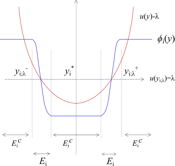
Next, we define functions which change sign near the spectral parameter , and have transition layer adapted to the set .
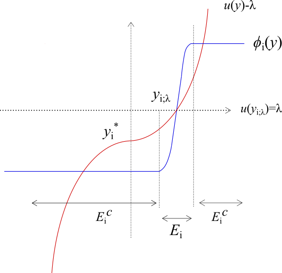
Given the shear profile we first define the such that . If the vanishing order of the critical point is odd, then there are two points such that . In this case, we use and to represent them and use to denote the set .
Since the balls are mutually disjoint, the associated with different critical points are distinct. We define the function :
(3.72)
(3.73)
(3.74)
(3.75)
(3.76)
(3.77)
Since the function is very similar to the function in the proof of Lemma 3.3, the regularity estimates are similar to those of . Here the universal constant is chosen such that if , then . By the estimate of on the support of (3.2), the existence of this universal constant , which is independent of , is guaranteed.
Figure 1. Function for odd(left). Function for even (right).
Now we estimate the area of the set . Based on the relative position between and , we distinguish between two cases:
(3.78)
In case (3.78), we first consider the case where the vanishing order is even. As a result, the shear profile is strictly monotone near the critical point and there is a unique such that . We consider arbitrary (3.68). Note that in this case, the product . Application of the mean value theorem, the -estimates (3.2), (3.3) on the support of and definition of (3.68) yields that
(3.79)
(3.80)
Since the estimate holds for all , we have that
(3.81)
If the vanishing order is odd, then . Now we define .
Now carrying out similar argument yields (3.81).
In the case (3.78), by picking small enough in the definition of the set (3.68), we have that for , the following the derivative lower bound of holds,
(3.82)
Combining this derivative lower bound and a similar argument to (3.80) yields that .
To conclude step #1, we estimate a specific function which will be applied later. We first consider the case where is even. We apply the properties of the functions and the mean value theorem to estimate the following function for ,
(3.83)
(3.84)
Now by the behavior of the shear profile on the support of (3.2), (3.3), the constraint (3.18), the definition of (3.68), we observe that
(3.85)
(3.86)
(3.87)
Combining the lower bound, the estimate (3.84) and the property b) of the function , we have obtained the following
(3.88)
Here if is odd, then we can replace the above by either or . Moreover, we will decompose the domain into the three subdomains , , where denotes the connect component of which contains . Application of similar estimate above yields the estimate (3.88). This concludes step #1.
Step #2: Estimation of . Direct application of the constraint (3.68) and property a) of the function yields that
Now we apply the bound (3.88), property a) and c) of the functions and the product estimate (3.42), Hölder inequality, Young’s inequality and Gagliardo-Nirenberg interpolation inequality to get the following
(3.91)
(3.92)
(3.93)
(3.94)
(3.95)
(3.96)
(3.97)
Note that the second term on the right hand side gets absorbed by the left hand side, which implies the following estimate
(3.98)
(3.99)
Combining this relation with (3.89) and the properties of the function yields the following
(3.100)
(3.101)
(3.102)
Now we estimate each term in (3.102). Combining the estimate (3.88) and the relation (3.5), we obtain
(3.103)
Now we estimate term with the relation (3.5) as follows
(3.104)
Next we estimate . The estimate of is similar to the estimate of (3.65) in the proof of Lemma 3.3. Combining the property b) of the function , the relation (3.5), Gagliardo-Nirenberg inequality, and Young inequality, we obtain
(3.105)
Combining the estimates (3.103), (3.104), (3.105) and the relation (3.102), we obtain the estimate
(3.106)
This concludes step #2.
Step #3: Estimation of (3.68).
Applying the area estimate (3.81), the relation (3.5), Gagliardo-Nirenberg interpolation inequality and Young inequality, we estimate the contribution as follows:
(3.107)
(3.108)
(3.109)
(3.110)
(3.111)
Combining (3.111) and estimate (3.106) implies (3.15) for .
∎
Assume the conditions in Theorem 1. For (3.19), the estimate (3.15) holds for small enough.
Proof.
Combining the assumption and the fact that the derivative is away from zero in the region , we have that for . Now we apply the relation (3.7) with , the product estimate (3.42), the Gagliardo-Nirenberg interpolation inequality and Young inequality to obtain that
(3.112)
(3.113)
(3.114)
(3.115)
for any positive constant . This implies the estimate (3.15).
∎
Finally, we estimate
Lemma 3.6.
Assume the condition in Theorem 1. Then the following estimate holds for any positive constant and small enough,
(3.116)
Proof.
Note that on the support of , the function intersects the value at different points , and near each intersection, the derivative of is away from zero, i.e., . We use the transition function trick again. To this end, we consider the following transition function :
(3.117)
(3.118)
(3.119)
(3.120)
Now we focus on one intersection and comment that other intersections are similar. We test the equation (2.8) with and obtain the following relation
(3.121)
We further decompose the domain into the following two component:
a) ; b) .
To estimate the solution on , we apply the Gagliardo-Nirenberg interpolation inequality inequality and to obtain:
(3.122)
(3.123)
(3.124)
(3.125)
Now we estimate the component of the solution. To this end, we collect the relation (3.121), the fact that is bounded below on the set , and the fact that on . Then we apply the product estimate (3.42), the Gagliardo-Nirenberg interpolation inequality to estimate the part as follows,
(3.126)
(3.127)
(3.128)
(3.129)
(3.130)
We estimate each term in the expression (3.130). Before estimating the term, we apply property c) of the function , the fact that the derivative of does not vanish in the set to derive the following relation
(3.131)
(3.132)
The estimate yields that
(3.133)
Now we estimate in the decomposition using Hölder inequality, Young’s inequality and the estimate (3.5), as follows
(3.134)
Finally, we estimate in (3.130). We estimate the -norm of . By the Gagliardo-Nirenberg interpolation inequality and the regularity of (3.118), we have the following estimate
(3.135)
Combining these two estimate together with Hölder inequality, Young’s inequality and the estimate (3.5), we obtain that for ,
We combine Lemma 3.3, Lemma 3.4, Lemma 3.5, and Lemma 3.6, to obtain that if for chosen in (3.27), the following estimate holds
(3.138)
(3.139)
If we choose , and then small enough, then for , the following estimate holds
(3.140)
Combining the -estimate with the relation (3.5)
yields the conclusion (2.10). Recalling Lemma 3.1, this completes the proof of Proposition 2.1.
∎
References
[1]
G. Alberti, G. Crippa, and A. L. Mazzucato.
Exponential self-similar mixing and loss of regularity for continuity
equations.
C. R. Math. Acad. Sci. Paris, 352(11):901–906, 2014.
[2]
G. Alberti, G. Crippa, and A. L. Mazzucato.
Exponential self-similar mixing by incompressible flows.
J. Amer. Math. Soc., 32(2):445–490, 2019.
[3]
M. Beck and C. Wayne.
Metastability and rapid convergence to quasi-stationary bar states
for the two-dimensional Navier–Stokes equations.
Proc. Royal Soc. of Edinburgh: Sec. A Mathematics,
143(05):905–927, 2013.
[4]
J. Bedrossian.
Suppression of plasma echoes and Landau damping in Sobolev spaces
by weak collisions in a Vlasov-Fokker-Planck equation.
Ann. PDE, 3(2):Paper No. 19, 66, 2017.
[5]
J. Bedrossian.
Nonlinear echoes and Landau damping with insufficient regularity.
Tunis. J. Math., 3(1):121–205, 2021.
[6]
J. Bedrossian and M. Coti Zelati.
Enhanced dissipation, hypoellipticity, and anomalous small noise
inviscid limits in shear flows.
Arch. Ration. Mech. Anal., 224(3):1161–1204, 2017.
[7]
J. Bedrossian, P. Germain, and N. Masmoudi.
Dynamics near the subcritical transition of the 3D Couette flow II:
Above threshold.
arXiv:1506.03721, 2015.
[8]
J. Bedrossian, P. Germain, and N. Masmoudi.
On the stability threshold for the 3D Couette flow in Sobolev
regularity.
Ann. of Math. (2), 185(2):541–608, 2017.
[9]
J. Bedrossian, P. Germain, and N. Masmoudi.
Dynamics near the subcritical transition of the 3D Couette flow I:
Below threshold.
Mem. Amer. Math. Soc., 266(1294):v+158, 2020.
[10]
J. Bedrossian and S. He.
Inviscid damping and enhanced dissipation of the boundary layer for
2d Navier-Stokes linearized around couette flow in a channel.
arXiv:1909.07230.
[11]
J. Bedrossian and S. He.
Suppression of blow-up in Patlak-Keller-Segel via shear flows.
SIAM Journal on Mathematical Analysis, 50(6):6365–6372, 2018.
[12]
J. Bedrossian and N. Masmoudi.
Inviscid damping and the asymptotic stability of planar shear flows
in the 2D Euler equations.
Publications mathématiques de l’IHÉS, pages 1–106,
2013.
[13]
J. Bedrossian, N. Masmoudi, and C. Mouhot.
Landau damping: paraproducts and Gevrey regularity.
Ann. PDE, 2(1):Art. 4, 71, 2016.
[14]
J. Bedrossian, N. Masmoudi, and V. Vicol.
Enhanced dissipation and inviscid damping in the inviscid limit of
the Navier-Stokes equations near the 2D Couette flow.
Arch. Rat. Mech. Anal., 216(3):1087–1159, 2016.
[15]
Q. Chen, T. Li, D. Wei, and Z. Zhang.
Transition threshold for the 2-D Couette flow in a finite
channel.
Arch. Ration. Mech. Anal., 238(1):125–183, 2020.
[16]
M. Colombo, M. C. Zelati, and K. Widmayer.
Mixing and diffusion for rough shear flows.
[17]
P. Constantin, A. Kiselev, L. Ryzhik, and A. Zlatoš.
Diffusion and mixing in fluid flow.
Ann. of Math. (2), 168(2):643–674, 2008.
[18]
M. Coti Zelati, M. G. Delgadino, and T. M. Elgindi.
On the relation between enhanced dissipation timescales and mixing
rates.
Comm. Pure Appl. Math., 73(6):1205–1244, 2020.
[19]
M. Coti-Zelati, M. Dolce, Y. Feng, and A. L. Mazzucato.
Global existence for the two-dimensional Kuramoto-Sivashinsky
equation with a shear flow.
arXiv:2103.02971, 2021.
[20]
M. Coti-Zelati and T. D. Drivas.
A stochastic approach to enhanced diffusion.
arXiv:1911.09995v1, 2019.
[21]
M. Coti Zelati, T. M. Elgindi, and K. Widmayer.
Enhanced dissipation in the Navier-Stokes equations near the
Poiseuille flow.
Comm. Math. Phys., 378(2):987–1010, 2020.
[22]
S. Ding and Z. Lin.
Enhanced dissipation and transition threshold for the 2-D plane
Poiseuille flow via resolvent estimate.
arXiv:2008.10057, 2020.
[23]
T. M. Elgindi and A. Zlatos.
Universal mixers in all dimensions.
Adv. Math., 356:106807, 33, 2019.
[24]
Y. Feng, Y. Feng, G. Iyer, and J.-L. Thiffeault.
Phase separation in the advective Cahn-Hilliard equation.
J. Nonlinear Sci., 30(6):2821–2845, 2020.
[25]
Y. Feng and G. Iyer.
Dissipation enhancement by mixing.
Nonlinearity, 32(5):1810–1851, 2019.
[26]
Y. Gong, S. He, and A. Kiselev.
Random search in fluid flow aided by chemotaxis.
arXiv:2107.02913, 2021.
[27]
S. He.
Suppression of blow-up in parabolic-parabolic Patlak-Keller-Segel
via strictly monotone shear flows.
Nonlinearity, 31(8):3651–3688, 2018.
[28]
K. Hopf and J. L. Rodrigo.
Aggregation equations with fractional diffusion: preventing
concentration by mixing, 2018.
[29]
L. Hörmander.
Hypoelliptic second order differential equations.
Acta Math., 119:147–171, 1967.
[30]
S. Ibrahim, Y. Maekawa, and N. Masmoudi.
On pseudospectral bound for non-selfadjoint operators and its
application to stability of Kolmogorov flows.
Ann. PDE, 5(2):Paper No. 14, 84, 2019.
[31]
G. Iyer, A. Kiselev, and X. Xu.
Lower bounds on the mix norm of passive scalars advected by
incompressible enstrophy-constrained flows.
Nonlinearity, 27(5):973–985, 2014.
[32]
G. Iyer, X. Xu, and A. Zlatos.
Convection-induced singularity suppression in the keller-segel and
other non-linear pdes.
arXiv:1908.01941.
[33]
A. Kiselev and X. Xu.
Suppression of chemotactic explosion by mixing.
Arch. Ration. Mech. Anal., 222(2):1077–1112, 2016.
[34]
A. Kolmogoroff.
Zufällige Bewegungen (zur Theorie der Brownschen
Bewegung).
Ann. of Math. (2), 35(1):116–117, 1934.
[35]
A. N. Kolmogorov.
On dynamical systems with an integral invariant on the torus.
Doklady Akad. Nauk SSSR (N.S.), 93:763–766, 1953.
[36]
H. Li and W. Zhao.
Metastability for the dissipative quasi-geostrophic equation and the
non-local enhancement.
arXiv:2107.10594, 2021.
[37]
T. Li, D. Wei, and Z. Zhang.
Pseudospectral bound and transition threshold for the 3D
Kolmogorov flow.
Comm. Pure Appl. Math., 73(3):465–557, 2020.
[38]
P. Malliavin.
Stochastic analysis, volume 313 of Grundlehren der
Mathematischen Wissenschaften [Fundamental Principles of Mathematical
Sciences].
Springer-Verlag, Berlin, 1997.
[39]
C. Mouhot and C. Villani.
On Landau damping.
Acta Math., 207:29–201, 2011.
[40]
D. Nualart.
The Malliavin calculus and related topics.
Probability and its Applications (New York). Springer-Verlag, Berlin,
second edition, 2006.
[41]
V. Romanov.
Stability of plane-parallel couette flow.
Funct. anal. and appl., 7(2):137–146, 1973.
[42]
C. Seis.
Maximal mixing by incompressible fluid flows.
Nonlinearity, 26(12):3279–3289, 2013.
[43]
T. Tao.
Nonlinear dispersive equations, volume 106 of CBMS
Regional Conference Series in Mathematics.
Published for the Conference Board of the Mathematical Sciences,
Washington, DC; by the American Mathematical Society, Providence, RI, 2006.
Local and global analysis.
[44]
C. Villani.
Hypocoercivity.
American Mathematical Soc., 2009.
[45]
J. von Neumann.
Zur Operatorenmethode in der klassischen Mechanik.
Ann. of Math. (2), 33(3):587–642, 1932.
[46]
D. Wei.
Diffusion and mixing in fluid flow via the resolvent estimate.
Science China Mathematics, pages 1–12, 2019.
[47]
D. Wei, Z. Zhang, and W. Zhao.
Linear inviscid damping for a class of monotone shear flow in
Sobolev spaces.
Preprint, arxiv:1509.08228, 2015.
[48]
Y. Yao and A. Zlatos.
Mixing and un-mixing by incompressible flows.
J. Eur. Math. Soc. (JEMS), 19(7):1911–1948, 2017.
[49]
C. Zillinger.
Linear inviscid damping for monotone shear flows.
arXiv preprint arXiv:1410.7341, 2014.