Improvement of phase sensitivity in SU(1,1) interferometer via a Kerr nonlinear

Abstract

We propose a theoretical scheme to enhance the phase sensitivity by introducing a Kerr nonlinear phase shift into the traditional SU(1,1) interferometer with a coherent state input and homodyne detection. We investigate the realistic effects of photon losses on phase sensitivity and quantum Fisher information. The results show that compared with the linear phase shift in SU(1,1) interferometer, the Kerr nonlinear case can not only enhance the phase sensitivity and quantum Fisher information, but also significantly suppress the photon losses. We also observe that at the same accessible parameters, internal losses have a greater influence on the phase sensitivity than the external ones. It is interesting that, our scheme shows an obvious advantage of low-cost input resources to obtain higher phase sensitivity and larger quantum Fisher information due to the introduction of nonlinear phase element.

PACS: 03.67.-a, 05.30.-d, 42.50,Dv, 03.65.Wj

I Introduction

Quantum metrology has a close relation to various-important information areas, such as Bose-Einstein condensate 1 ; 2 ; 3 , gravitational wave detection 4 ; 5 , and quantum imaging 6 ; 7 ; 8 . It has been widely concerned and highly developed in recent years. To meet the high precision demand, all kinds of optical interferometers have been proposed. For instance, as a general model, the Mach–Zehnder interferometer (MZI) has been used to be an essential tool to provide insight into tiny variations on phase shift 9 ; 10 ; 11 .

In order to improve the precise measurement, generally speaking, we can focus on the following three stages 12 : probe generation 13 ; 14 ; 15 ; 16 , probe modification 17 ; 18 ; 19 ; 20 ; 21 and probe readout 22 ; 23 , as illustrated in Fig. 1(a). In particular, for the probe generation, the phase sensitivity is always confined to the standard quantum limit (SQL) when the classical resources are injected into the input ports of the MZI. To surpass the SQL, non-classical quantum states have widely used as the input of the MZI, such as entangled states 13 , twin Fock states 24 , and NOON states 25 , by which the Heisenberg limit (HL) even can be reached 26 ; 27 . Although the usage of nonclassical states can greatly improve the phase sensitivity of optical interferometers, these states with large average photon numbers are not only more difficult to prepare, but also very fragile especially in the presence of environmental interferences 28 ; 29 ; 30 . Thus, from the viewpoint of resource theory, it will be a challenging task with simple input state (such as coherent state (CS)) to further improve the precision of measurement, especially in the realistic case.

On the other hand, many efforts have been paid to the stage of probe modification, especially when Yurke et al. first proposed an SU(1,1) interferometer with a linear phase shift 20 . In this system, the active nonlinear optical devices, such as four-wave mixers (FWMs) and optical parametric amplifiers (OPAs), are used instead of the passive linear beam splitters (BSs) used in the conventional MZI 31 ; 32 ; 33 ; 34 ; 35 ; 36 ; 37 . To beat the SQL, Plick et al. applied strong CS as the inputs into the SU(1,1) interferometer 33 . Subsequently, Li et al. proposed a scheme of reaching HL sensitivity via a squeezed vacuum state (SVS) plus a CS with the homodyne detection 31 . It is interesting that, Hudelist et al. pointed out that the signal-to-noise ratio (SNR) of the SU(1,1) interferometer is about 4.1 dB higher than that of the MZI under the same phase-sensing intensity 38 . This point may be one of reasons focusing on this interferometer. Actually, this implies the role of nonlinear process for improving the precision.

Expect the SU(1,1) nonlinear process, the nonlinear phase shifts have also been proposed for enhancing the phase estimation, which can be viewed as another way of the probe modification 9 ; 39 ; 40 ; 41 ; 42 . For instance, in the traditional MZI, Zhang et al. investigated the phase estimation by replacing linear phase shift by nonlinear one 9 using a CS and parity measurement. Jiao et al. proposed an improved protocol of nonlinear phase estimation by inserting a nonlinear phase shift into the traditional MZI, with active correlation output readout and homodyne detection 39 . More recently, Chang et al. suggested a scheme for enhancing phase sensitivity by introducing nonlinear phase shifter to the modified interferometer consisting of a balanced BS and an optical parameter amplifier (OPA) 41 . It is shown that the OPA potential can be stimulated by nonlinear phase shifter, which is absent for the case of linear phase shifter. In addition, the estimation of nonlinear phase has also lots of applications, such as the third-order susceptibility of the Kerr medium 39 , phase-sensitive amplifiers 43 ; 44 and nonclassical quantum state preparations 45 ; 46 . These results show that the nonlinear optical devices can be considered as powerful tools to effectively achieve both high accuracy and sensitivity. However, on one hand, the researches on nonlinear phase estimation are not as systematic as those on linear one. On the other, most works on the phase precision are based on either specific measurement, especially in the presence of photon loss, or direct calculation of quantum Fisher information for ideal case.

In this paper, we mainly focus on the nonlinear phase estimation of a Kerr SU(1,1) (KSU(1,1)) interferometer by replacing the linear phase shift with the Kerr nonlinear one, together with CS plus vacuum state (VS) (denoted as $\left|\alpha\right\rangle_{a}\otimes\left|0\right\rangle_{b}$) as inputs and homodyne detection. Both the phase sensitivity and the quantum Fisher information (QFI) are analytically investigated with and without photon losses. The phase sensitivity can beat the SQL and approach the HL. Compared to the traditional SU(1,1) interferometer with a linear phase and other inputs resources including CS+CS and SVS+CS, our scheme presents much QFI and higher phase sensitivity closer to the quantum Cramér-Rao (QCRB) 34 ; 47 ; 48 ; 49 ; 50 . From the viewpoint of resource theory, CS+VS can be seen as the most simple and easily available input, thus our scheme has an obvious advantage of low-cost input by inserting nonlinear phase shift into the SU(1,1) interferometer.

The remainder of this paper is arranged as follows. Section II introduces the KSU(1,1) interferometer in our scheme. In Section III, we investigate the phase sensitivity of the output signal with homodyne detection, and compare them with the conventional SU(1,1) interferometer. In Section IV, we get the QFI of Kerr nonlinear phase shift for the KSU(1,1) interferometer by invoking the characteristic function (CF) approach. In Section V, we discuss the effects of photon losses on both phase sensitivity and QFI of Kerr nonlinear phase shift, respectively. Conclusions are made in the last section.

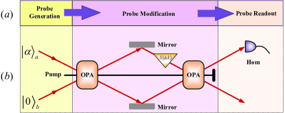
Figure 1: (Color online) (a) The general process of estimating an unknown parameter $\phi$. (b) Schematic diagram of SU(1,1) interferometer with a nonlinear phase shifter $S\left(\phi,k\right).$ The two input ports of this interferometer are a coherent state $\left|\alpha\right\rangle_{a}$ and a vacuum state $\left|0\right\rangle_{b},$ respectively. OPA is an optical parametric amplifier and Hom is a homodyne detection.

II Nonlinear phase estimation model

Let us begin with the description of nonlinear phase estimation model, as shown in Fig. 1(b). The nonlinear interferometer consists of two OPAs (or FWMs) and a Kerr-type medium. Here we consider a CS $\left|\alpha\right\rangle_{a}$ with $\alpha=\left|\alpha\right|e^{i\theta_{\alpha}}$ and a VS $\left|0\right\rangle_{b}$ as the inputs in mode $a$ and mode $b$, respectively. Thus the probing state can be shown as $\left|\psi_{in}\right\rangle=$ $\left|\alpha\right\rangle_{a}\otimes\left|0\right\rangle_{b}.$ After going through the first OPA, the resulting state is given by $\hat{S}\left(\xi_{1}\right)\left|\psi_{in}\right\rangle$ i.e., a two-mode squeezed CS, where the operator $\hat{S}\left(\xi_{1}\right)=\exp(\xi_{1}^{\ast}\hat{a}\hat{b}-\xi_{1}\hat{a}^{\dagger}\hat{b}^{\dagger})$ represents the OPA process, $\xi_{1}=g_{1}e^{i\theta_{1}}$, with a gain factor $g_{1}$ and a phase shift $\theta_{1}$ and $\hat{a}(\hat{a}^{\dagger}),\hat{b}(\hat{b}^{\dagger})$ are the annihilation (creation) operators, for modes $a$ and $b$, respectively. For simplicity, we assume that the Kerr-type medium is inset into the path $b$ between the first and second OPAs to generate a nonlinear phase shift $\phi$ to be estimated.

After the interaction between the state $\hat{S}\left(\xi_{1}\right)\left|\psi_{in}\right\rangle$ with the Kerr-type medium, the corresponding modified state becomes

$$\left|\psi_{\phi}\right\rangle=\hat{S}\left(\phi,k\right)\hat{S}\left(\xi_{1}\right)\left|\psi_{in}\right\rangle,$$ (1)

depending on the phase parameter $\phi$, where

$$\hat{S}\left(\phi,k\right)=e^{i\phi(\hat{b}^{\dagger}\hat{b})^{k}},$$ (2)

is the nonlinear phase shift operator and the exponent $k$ is the order of the nonlinearity. In particular, for the case of $k=1$, $\hat{S}\left(\phi,1\right)=e^{i\phi\hat{b}^{\dagger}\hat{b}}$ just reduces to the linear phase shift, while for the case of $k=2$, $\hat{S}\left(\phi,2\right)=e^{i\phi(\hat{b}^{\dagger}\hat{b})^{2}}$ corresponds to Kerr nonlinear case. Throughout this paper, we only consider both Kerr-type nonlinear medium and linear one by taking $k=1,2$, respectively.

After the second OPA, the final output state is given by

$$\left|\psi_{out}\right\rangle=\hat{S}\left(\xi_{2}\right)\hat{S}\left(\phi,k\right)\hat{S}\left(\xi_{1}\right)\left|\psi_{in}\right\rangle,$$ (3)

where $\hat{S}\left(\xi_{2}\right)=\exp(\xi_{2}^{\ast}\hat{a}\hat{b}-\xi_{2}\hat{a}^{\dagger}\hat{b}^{\dagger}),$ with $\xi_{2}=g_{2}e^{i\theta_{2}},$ is a two-mode squeezing operator, corresponding to the second OPA process. The Kerr nonlinear phase shifter $\hat{S}\left(\phi,2\right)$ satisfying the transformation relation:

$$\hat{S}^{\dagger}\left(\phi,2\right)\hat{b}^{\dagger}\hat{S}\left(\phi,2\right)=e^{-i\phi}\hat{b}^{\dagger}e^{-i2\phi\hat{b}^{\dagger}\hat{b}},$$ (4)

which is useful for the calculation of phase sensitivity. One can refer to Appendix A about more details of derivation for this relation. Finally, the homdyne detection is performed on mode $a$, so that one can read information about the value of $\phi$.

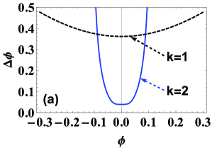
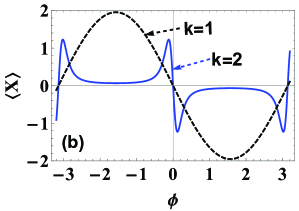
Figure 2: (Color online) (a) Phase sensitivity based on homodyne detection and (b) the output signal as a function of $\phi$ with $g=1$, $\left|\alpha\right|=1$, and $\theta_{\alpha}=\frac{\pi}{2}$. The black-dashed line and the blue-solid line correspond to the linear phase shift ($k=1$) and the Kerr nonlinear phase shift ($k=2$), respectively.

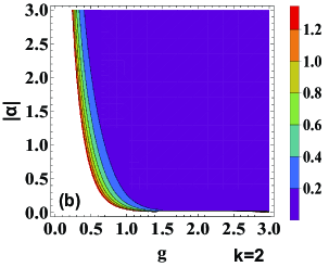
Figure 3: (Color online) Phase sensitivity based on homodyne detection as a function of the gain factor $g$ and the coherent amplitude $\left|\alpha\right|$ with $\theta_{\alpha}=\pi/2$ and $\phi=0$ for (a) the linear phase shift ($k=1$), and (b) the Kerr nonlinear phase shift ($k=2$), respectively.

III Phase sensitivity via homodyne detection

Next, we investigate the phase sensitivity of nonlinear phase. For this purpose, we need to choose a special detection method for the readout of phase information at the final output port. Actually, there are many different detection methods, such as homodyne detection 11 ; 31 ; 32 , intensity detection 33 ; 34 ; 47 , and parity detection 27 ; 35 ; 36 . Each way of measurement has its own advantages. For example, the parity detection has been proved to be an optimal detection for linear phase estimation in lots of schemes 27 ; 51 . Compared with both intensity and parity detections, however, homodyne detection can be easily realized with current technologies, thereby playing a key role in the field of continuous-variable quantum key distribution (CV-QKD) 52 ; 53 ; 54 ; 55 ; 56 . Therefore, in our scheme the homodyne detection is employed on mode $a$ at one of output port to estimate the phase parameter $\phi,$ where the detected variable is the amplitude quadrature $\hat{X}$, i.e.,

$$\hat{X}=(\hat{a}+\hat{a}^{\dagger})/\sqrt{2}.$$ (5)

Based on the error propagation formula, the phase sensitivity can be calculated by

$$\Delta\phi=\frac{\sqrt{\Delta^{2}\hat{X}}}{\left|\partial\left\langle\hat{X}\right\rangle/\partial\phi\right|},$$ (6)

with $\Delta^{2}\hat{X}=\left\langle\hat{X}^{2}\right\rangle-\left\langle\hat{X}\right\rangle^{2}.$ According to Eq. (6), for an arbitrary value of $\phi$, the corresponding phase sensitivity can be analytically derived. For simplicity, the corresponding expression is not shown here. One can refer to Appendix B for more details. In the following discussions, we assume that the KSU(1,1) interferometer is in a balanced situation, i.e., $\theta_{2}-\theta_{1}=\pi$ and $g_{1}=g_{2}=g.$

In Fig. 2(a), we show the phase sensitivity changing with $\phi$ for the linear ($k=1$) and nonlinear ($k=2$) phase shifts when given parameters $g=1,|\alpha|=1,$and $\theta_{\alpha}=\pi/2.$ It is clearly seen that, for both cases above, the minimum value of the phase sensitivity can be achieved at the optimal point $\phi=0.$ In addition, the phase sensitivity for $k=2$ is always significantly superior to that for $k=1$ around the optimal point. This implies that the nonlinear phase shift can be further used to improve the phase sensitivity, compared to the linear one. The reason lies in that the introduction of nonlinear phase shift increases the slope $\partial\left\langle\hat{X}\right\rangle/\partial\phi$ of the output signal $\left\langle\hat{X}\right\rangle$ at $\phi=0,$ which leads to the increase of the denominator in Eq. (6), as shown in Fig. 2(b). In fact, this point will be clear by deriving the phase sensitivity $\Delta\phi_{k}$ for $k=1,2$ at $\phi=0$, which are given by

$$\Delta\phi_{1} =\frac{1}{\sqrt{N_{\alpha}}N_{OPA}},$$ (7)

$$\Delta\phi_{2} =\frac{\Delta\phi_{1}}{1+N_{OPA}\left(N_{\alpha}+2\right)},$$ (8)

where $\Delta\phi_{1}$ represents the phase sensitivity of the traditional SU(1,1) interferometer with a linear phase shift $k=1,$ $N_{\alpha}=\left|\alpha\right|^{2}$ is the mean photon number of the input coherent state, and $N_{OPA}=2\sinh^{2}g$ is the total photon number after the first OPA with vacuum inputs. Obviously, $\Delta\phi_{2}>\Delta\phi_{1}.$

Moreover, from Fig. 2(b) it is shown that the peak width for the case of $k=2$ is narrower than that for the case of $k=1.$ In this sense, the nonlinear phase shift can also improve supperresolution compared to the linear one. On the other hand, to display the effects of both the coherence amplitude $\left|\alpha\right|$ and the gain factor $g$ on the phase sensitivity, at the optimal point $\phi=0,$ we also plot the phase sensitivity as a function of $\left|\alpha\right|$ and $g$ with different values of $k=1,2$, in Figs. 3(a) and 3(b), respectively. It is found that, the values of $\Delta\phi$ rapidly decrease with the increase of $\left|\alpha\right|$ and $g$, especially for the case of $k=2.$

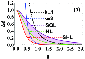
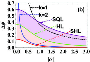
Figure 4: (Color online) Phase sensitivity based on homodyne detection as a function of (a) the gain factor $g$ with $\left|\alpha\right|=1$. (b) the coherent amplitude $\left|\alpha\right|$ with $g=1$ ($\theta_{\alpha}=\pi/2$ ). The black-dashed and blue-solid lines are respectively the linear phase shift ($k=1$), and the Kerr nonlinear phase shift ($k=2$), while the purple-, green- and red-solid lines respectively correspond to the SQL, HL and SHL.

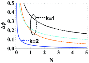
Figure 5: (Color online) Phase sensitivity based on homodyne detection as a function of the total average photon number N of input state with $g=1.$ The orange- and cyan-dot-dashed lines respectively correspond to a squeezed vacuum state combined with a coherent states input and two coherent states with the linear phase shift ($k=1$), as shown in Ref. 31 ; 32 ; while the black-dashed and blue-solid lines are respectively the linear phase shift ($k=1$), and the Kerr nonlinear phase shift ($k=2$).

To further show the advantage of our scheme, we also make a comparison about phase sensitivities, involving the SQL ($\Delta\phi\thicksim 1/\sqrt{N_{Total}}$), the HL ($\Delta\phi\thicksim 1/N_{Total}$) and the Super HL (SHL) ($\Delta\phi\thicksim 1/N_{Total}^{2}$), as shown in Fig. 4. Note that $N_{Total}=\left\langle\psi_{in}\right|\hat{S}^{\dagger}\left(\xi_{1}\right)(\hat{a}^{\dagger}\hat{a}+\hat{b}^{\dagger}\hat{b})\hat{S}\left(\xi_{1}\right)\left|\psi_{in}\right\rangle$ is the total mean photon number inside the KSU(1,1) interferometer. From Fig. 4, the black dashed line is the sensitivity performance of the linear phase shift, which can only break through SQL and is always surpassed by that of the Kerr nonlinear phase shift. In particular, the latter can break both the SQL and the HL, but cannot beat the SHL. The reason may be that adopting the Kerr nonlinear phase shift to effectively improve the maximum amount of information about the unknown phase shift $\phi$ can result in a transition from HL ($\Delta\phi\thicksim 1/N_{Total}$) to SHL ($\Delta\phi\thicksim 1/N_{Total}^{2}$), as described in Refs. 9 ; 57 ; 58 ; 59 ; 60 ; 61 ; 62 . Nevertheless, the common feature of these two is that the phase sensitivity increases with the increase of $\left|\alpha\right|$ and $g$.

Next, we make a comparison about the performance of phase sensitivity. In Fig. 5, the phase sensitivity is plotted as a function of the total average input photon number $N$ with several different input resources, including $\left|\alpha\right\rangle_{a}\otimes\left|\beta\right\rangle_{b}$, $\left|\alpha\right\rangle_{a}\otimes\left|\varsigma,0\right\rangle_{b}$ and $\left|\alpha\right\rangle_{a}\otimes\left|0\right\rangle_{b}$ used in the traditional SU(1,1) interferometer ($k=1$) and $\left|\alpha\right\rangle_{a}\otimes\left|0\right\rangle_{b}$ used in the KSU(1,1) interferometer ($k=2$). It is shown that, for the traditional case, the phase sensitivity with the input $\left|\alpha\right\rangle_{a}\otimes\left|0\right\rangle_{b}$ performs the worst among these three inputs 31 ; 32 . This implies that the introduction of coherence amplitude $\left|\alpha\right|$ or squeezing parameter $\varsigma$ is beneficial for the phase sensitivity improvement. However, for the KSU(1,1) interferometer, it is interesting that the best phase sensitivity can be achieved only using the simplest input $\left|\alpha\right\rangle_{a}\otimes\left|0\right\rangle_{b}$, which is significantly superior to those inputs in the traditional SU(1,1) interferometer. That is to say, for a simple input with less energy and less resources, the phase sensitivity can be further improved by introducing Kerr nonlinear phase.

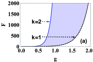
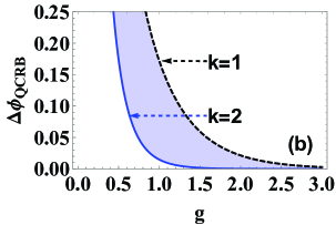
Figure 6: (Color online) (a) The quantum Fisher information $F$ and (b) the QCRB as a function of gain factor g for $\left|\alpha\right|=1$ ( $\theta_{\alpha}=\pi/2$), respectively. The black-dashed and blue-solid lines correspond to linear phase shift ($k=1$) and Kerr nonlinear phase shift ($k=2$), respectively.

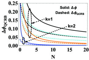
Figure 7: (Color online) The $\Delta\phi_{QCRB}$ as a function of the total average photon number N of input state with $g=1.$ The orange and cyan lines correspond to a coherent state plus a squeezed vacuum state input and two coherent states, respectively, with the linear phase shift ($k=1$); while the black and blue lines correspond to $k=1$, and the Kerr nonlinear phase shift ($k=2$), respectively. The dashed and solid lines correspond to the $\Delta\phi_{QCRB}$ and the $\Delta\phi,$ respectively.

IV The QFI in the KSU(1,1) interferometer

As an elegant approach, the QFI can be used to visually describe the maximum amount of information about the unknown phase shift $\phi$, which is connected with the QCRB. In fact, the QFI is the intrinsic information in quantum state and is independent of any specific detection scheme. In the absence of losses, for a pure state, the corresponding QFI can be calculated as 34 ; 48 ; 49

$$F=4\left[\left\langle\psi_{\phi}^{\prime}|\psi_{\phi}^{\prime}\right\rangle-\left|\left\langle\psi_{\phi}^{\prime}|\psi_{\phi}\right\rangle\right|^{2}\right],$$ (9)

where $\left|\psi_{\phi}\right\rangle=\hat{S}\left(\phi,k\right)\hat{S}\left(\xi_{1}\right)\left|\psi_{in}\right\rangle$ is the state vector prior to the second OPA and $\left|\psi_{\phi}^{\prime}\right\rangle=\partial\left|\psi_{\phi}\right\rangle/\partial\phi.$ Then, for the linear phase shift $\left(k=1\right)$ and the Kerr nonlinear phase shift $\left(k=2\right),$ the QFI can be, respectively, reformed as 45

$$F_{1}=4\left\langle\Delta^{2}\hat{n}\right\rangle,F_{2}=4\left\langle\Delta^{2}\hat{n}^{2}\right\rangle,$$ (10)

where $\hat{n}=\hat{b}^{\dagger}\hat{b}$ is the photon number operator on mode $b$ and $\left\langle\Delta^{2}\hat{n}^{j}\right\rangle=$ $\left\langle\bar{\psi}_{out}\right|\left(\hat{n}^{j}\right)^{2}\left|\bar{\psi}_{out}\right\rangle-\left\langle\bar{\psi}_{out}\right|\hat{n}^{j}\left|\bar{\psi}_{out}\right\rangle^{2},\left(j=1,2\right)$ with the state vector after the first OPA, i.e., $\left|\bar{\psi}_{out}\right\rangle=\hat{S}\left(\xi_{1}\right)\left|\psi_{in}\right\rangle.$ Using the normal ordering forms of the operators,

$$(\hat{b}^{\dagger}\hat{b})^{4} =\hat{b}^{\dagger 4}\hat{b}^{4}+6\hat{b}^{\dagger 3}\hat{b}^{3}+7\hat{b}^{\dagger 2}\hat{b}^{2}+\hat{b}^{\dagger}\hat{b},$$

$$(\hat{b}^{\dagger}\hat{b})^{2} =\hat{b}^{\dagger 2}\hat{b}^{2}+\hat{b}^{\dagger}\hat{b},$$ (11)

and the characteristic function method for calculating average, it is ready to have

$$F_{1}=4\left(\bar{A}_{2}+\bar{A}_{1}-\bar{A}_{1}^{2}\right),F_{2}=F_{1}+f,$$ (12)

with

$$f =4\left[\bar{A}_{4}+6\left(\bar{A}_{3}+\bar{A}_{2}\right)-\bar{A}_{2}\left(\bar{A}_{2}+2\bar{A}_{1}\right)\right],$$ (13)

$$\bar{A}_{m} =m!(\sinh^{2m}g)L_{m}(-\left|\alpha\right|^{2}),m\in\{1,2,3,4\},$$ (14)

and $L_{m}(\bullet)$ is the Laguerre polynomials. One can refer to Appendix C for more details about derivations of $\bar{A}_{m}$. Based on Eq. (12), we can give the QCRB $\Delta\phi_{QCRB},$ which represents the lower bound of the phase sensitivity, i.e.,

$$\Delta\phi_{QCRB}=\frac{1}{\sqrt{\upsilon F_{k}}},\text{ }\left(k=1,2\right),$$ (15)

where $\upsilon$ is the number of trials. For simplicity, here we set $\upsilon=1.$ In general, the smaller the values of $\Delta\phi_{QCRB}$, the higher the phase sensitivity.

To clearly see this point, according to Eqs. (12) and (15), at a fixed $\left|\alpha\right|=1,$ Fig. 6 shows the QFI and the QCRB changing with $g$ for different $k=1,2.$ It is clear that, for the cases of $k=1,2,$ the values of the QFI increase significantly with the increase of $g,$ thereby leading to the more precise phase sensitivity. Moreover, when given the same gain factor $g$, both the QFI and the QCRB of $k=2$ always outperform those of $k=1$, which distinctly shows the superiority of the nonlinear phase shift compared to the linear case. This result originates from the additional item $f$ in Eq. (12), giving rise to the increase of QFI.

As a comparison, we also consider the $\Delta\phi_{QCRB}$ as a function of $N$ for several different input resources in Fig. 7, similar to the phase sensitivity (in Fig. 5). Some similar results are obtained. For instance, although the QCRB with $\left|\alpha\right\rangle_{a}\otimes\left|0\right\rangle_{b}$ is the worst than that with other resources in the traditional SU(1,1) interferometer 63 , the smallest $\Delta\phi_{QCRB}$ can be realized by the simplest input $\left|\alpha\right\rangle_{a}\otimes\left|0\right\rangle_{b}$ in the KSU(1,1) interferometer. In addition, comparing Fig. 5 with Fig. 7, it is found that compared with several different input resources in the traditional SU(1,1) interferometer, the input $\left|\alpha\right\rangle_{a}\otimes\left|0\right\rangle_{b}$ in the KSU(1,1) interferometer is closer to the ultimate phase precision $\Delta\phi_{QCRB}.$

V The effects of photon losses

In the realistic scenario, the decoherence process is unavoidable because there always exist interaction between the interferometer system and its surrounding environment, thereby leading to the information leakage from the system to the environment. For this season, the system performance would drop severely. In general, there are many types of decoherence process 64 ; 65 , such as photon loss, imperfect detector, phase diffusion, and so on. Here, for simplicity, we only study the effects of photon losses on both the phase sensitivity and the QFI in our scheme.

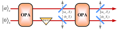
Figure 8: (Color online) Schematic diagram of the photon losses that occur before and after the second OPA. $T_{j}\left(j=1,2\right)$ is the transmissivity of the fictitious beam splitters; $a_{v_{j}}$ and $b_{v_{j}}$ are the vacuum noise operators.

V.1 The effects of photon losses on the phase sensitivity

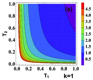
Figure 9: (Color online) Phase sensitivity based on homodyne detection as a function of the photon losses inside the interferometer $T_{1}$ and the photon losses outside the interferometer $T_{2}$ with $g=1$ and $\left|\alpha\right|=1$ ($\theta_{\alpha}=\pi/2$). (a) and (b) correspond to the cases with$k=1,2$, respectively.

Figure 10: (Color online) The output signal as a function of $\phi$ with $g=1$, $\left|\alpha\right|=1$, $\theta_{\alpha}=\frac{\pi}{2},$and $T_{1}=T_{2}=0.6$. The black and blue lines correspond to $k=1,2$, respectively. The dashed and solid lines correspond to the effects of photon losses and no photon losses, respectively.

First, let us consider the effects of photon losses before and after the second OPA on the phase sensitivity. Actually, the losses after the second OPA can also be seen as the detection imperfect at out ports. To describe the photon losses, the channel is usually simulated by inserting the fictitious beam splitter (BS_j) with transmissivity $T_{j}\left(j=1,2\right),$ as shown in Fig. 8. Generally speaking, the smaller the values of $T_{j}$, the more serious the photon loss. Here, we denote the photon loss inside and outside the interferometer as internal loss ($T_{1}$) and external one ($T_{2}$), respectively. In the following discussion, we assume that the losses of different modes are the same inside or outside the interferometer.

For any single-mode pure state $\left|\varphi\right\rangle_{in}$, after through the photon loss, the output state $\left|\varphi\right\rangle_{out}$ in an enlarged space can be expressed as a pure state, i.e., $\left|\varphi\right\rangle_{out}=\hat{U}_{BS_{j}}\left|\varphi\right\rangle_{in}\left|0\right\rangle$. Thus, the average value of operator $\hat{O}$ can be calculated as $\left\langle\hat{O}\right\rangle=\left.\left\langle 0\right|_{in}\left\langle\varphi\right|\right.\hat{U}_{BS_{j}}^{\dagger}\hat{O}\hat{U}_{BS_{j}}\left.\left|\varphi\right\rangle_{in}\left|0\right\rangle\right.$, which is equivalent to the average value in the reduced density operator $\rho_{out}=$Tr$[\hat{U}_{BS_{j}}\left|\varphi\right\rangle_{in}\left|0\right\rangle\left\langle 0\right|_{in}\left\langle\varphi\right|\hat{U}_{BS_{j}}^{\dagger}]$. In our scheme in Fig. 8, the final output state $\left|\varphi\right\rangle_{f}$ in the enlarged space is given by

$$\left|\varphi\right\rangle_{f}=\hat{U}_{BS_{2}}^{b}\hat{U}_{BS_{2}}^{a}\hat{S}\left(\xi_{2}\right)\hat{U}_{BS_{1}}^{b}\hat{U}_{BS_{1}}^{a}\left|\psi_{\phi}\right\rangle\left|\vec{0}\right\rangle,$$ (16)

where $\left|\vec{0}\right\rangle=\left|0000\right\rangle$ is the noise vacua, and $\hat{U}_{BS_{j}}^{a}=\exp[\arccos\sqrt{T_{j}}(\hat{a}^{\dagger}\hat{a}_{\upsilon_{j}}-\hat{a}\hat{a}_{\upsilon_{j}}^{\dagger})]$ and $\hat{U}_{BS_{l}}^{b}=\exp[\arccos\sqrt{T_{l}}(\hat{b}^{\dagger}\hat{b}_{\upsilon_{l}}-\hat{b}\hat{b}_{\upsilon_{l}}^{\dagger})]$ are the BS operators acting on mode $\hat{a}$ and $\hat{b}$, respectively. Here $\hat{a}_{\upsilon_{j}}$ and $\hat{b}_{\upsilon_{l}}$ are the vacuum noise operators.

Using the transformations of the fictitious BS_j on the annihilation operators, i.e.,

$$(\hat{U}_{BS_{j}}^{a})^{\dagger}\hat{a}\hat{U}_{BS_{j}}^{a} =\sqrt{T_{j}}\hat{a}+\sqrt{1-T_{j}}\hat{a}_{\upsilon_{j}},$$ (17)

$$(\hat{U}_{BS_{l}}^{b})^{\dagger}\hat{b}\hat{U}_{BS_{l}} =\sqrt{T_{l}}\hat{b}+\sqrt{1-T_{l}}\hat{b}_{\upsilon_{l}},$$ (18)

it is not difficult to obtain the phase sensitivity $\Delta\phi_{L_{k}}$ ($k=1,2$) after losses, not shown here for simplicity. In particular, at the optimal point $\phi=0,$ for the traditional and KSU(1,1) interferometers in the presence of photon loss, the phase sensitivities $\Delta\phi_{L_{k}}$ $(k=1,2)$ are derived, respectively, as

$$\Delta\phi_{L_{1}}=\sqrt{\left(\Delta\phi_{1}\right)^{2}+\frac{\left(1-T_{1}\right)T_{2}\cosh 2g+1-T_{2}}{4T_{1}T_{2}\left|\alpha\right|^{2}\sinh^{4}g}},$$ (19)

and

$$\Delta\phi_{L_{2}}=\frac{\Delta\phi_{L_{1}}}{1+N_{OPA}\left(N_{\alpha}+2\right)},$$ (20)

where the phase sensitivity $\Delta\phi_{L_{1}}$ corresponds to that of the traditional SU(1,1) interferometer in the presence of photon loss. In Eq. (19), the first term $\left(\Delta\phi_{1}\right)^{2}$ can be given by Eq. (8), while the second term is resulted from the internal and external losses. From Eqs. (19) and (20), it is obvious that $\Delta\phi_{L_{2}}>\Delta\phi_{L_{1}}\$in the presence of losses.

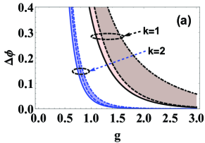
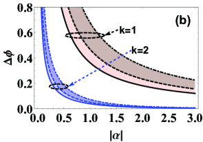
Figure 11: (Color online) Phase sensitivity based on homodyne detection as a function of (a) the gain factor $g$ with $\left|\alpha\right|=1$, (b) the coherent amplitude $\left|\alpha\right|$ with $g=1$ $(\theta_{\alpha}=\pi/2).$ The black and blue lines correspond to $k=1,2$, respectively. The dot-dashed line, dashed line, and solid line correspond to the photon losses inside the interferometer ($T_{1}=0.6$ and $T_{2}=1$), outside the interferometer ($T_{1}=1$ and $T_{2}=0.6$), and no photon losses ($T_{1}=$ $T_{2}=1$), respectively.

In order to visually see the influence of losses, at fixed values of $g=1$ and $\left|\alpha\right|=1,$ we plot the phase sensitivity $\Delta\phi_{L_{k}}$ $\left(k=1,2\right)$ as a function of $T_{j}\left(j=1,2\right)$ for different values of $k=1,2,$ as shown in Fig. 9. It is seen that for $k=1,2,$ the values of $\Delta\phi_{L_{k}}$ increase with the decrease of $T_{j},$ which shows that the phase sensitivity can be deeply influenced by the photon losses. Compared to the case of $k=1$ (Fig. 9(a)), the phase sensitivity of $k=2$ (Fig. 9(b)) is more robust against photon losses under the same conditions. The reason lies in that the Kerr nonlinear phase shift $\left(k=2\right)$ is beneficial to the increase of the denominator in the error propagation formula (see Fig. 10), thereby resulting in the improvement of the phase sensitivity even in the presence of the photon losses. In addition, from Fig. 10, it is also found that the full width of the main peaks for $k=2$ would broaden at fixed photon-loss factors $T_{j}=0.6$, which implies that the signal’s super-resolution characteristic is going to be worse. Even so, the usage of the Kerr nonlinear phase shift performs better than that of the linear one with respect to increasing the signal’s super-resolution.

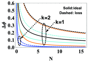
Figure 12: (Color online) Phase sensitivity based on homodyne detection as a function of the total average photon number N of input state with $g=1,$ $T_{1}=T_{2}=0.6.$ The orange- and cyan-dot-dashed lines respectively correspond to a squeezed vacuum state plus a coherent states input and two coherent states with $k=1$, as shown in Ref. 31 ; 32 ; The black and blue lines correspond to $k=1,2$, respectively. The dashed and solid lines correspond to the effects of photon losses and no photon losses, respectively.

Next, we consider their own effects of internal and external losses. From Eqs. (20) and (19), for the internal and external losses, the phase sensitivity $\Delta\phi_{L_{1}}$ and $\Delta\phi_{L_{2}}$ can be reduced, respectively, to

$$\left.\Delta\phi_{L_{1}}\right|_{T_{2}=1} =\sqrt{\left(\Delta\phi_{1}\right)^{2}+\frac{\left(1-T_{1}\right)\cosh 2g}{4T_{1}\left|\alpha\right|^{2}\sinh^{4}g}},$$ (21)

$$\left.\Delta\phi_{L_{2}}\right|_{T_{2}=1} =\frac{\left.\Delta\phi_{L_{1}}\right|_{T_{2}=1}}{1+N_{OPA}\left(N_{\alpha}+2\right)},$$ (22)

and

$$\left.\Delta\phi_{L_{1}}\right|_{T_{1}=1} =\sqrt{\left(\Delta\phi_{1}\right)^{2}+\frac{1-T_{2}}{4T_{2}\left|\alpha\right|^{2}\sinh^{4}g}},$$ (23)

$$\left.\Delta\phi_{L_{2}}\right|_{T_{1}=1} =\frac{\left.\Delta\phi_{L_{1}}\right|_{T_{1}=1}}{1+N_{OPA}\left(N_{\alpha}+2\right)}.$$ (24)

From Eqs. (21)-(24), it is clear that the effects of the internal losses are greater than those of the external ones on the phase sensitivity due to $\cosh\left(2g\right)>1$ for the same losses. To clearly see this point, Fig. 11 shows the phase sensitivity $\Delta\phi$ as a function of $\left|\alpha\right|$ or $g$ for the internal and external losses. It is shown that, for a fixed $k$, the gap between the ideal scenario and the internal-losses one is larger than that between the ideal scenario and the external-losses one. The gap increases first and then decreases, while the phase sensitivity still increases as the $\left|\alpha\right|$ or $g$ increases. It is interesting that, the gap for $k=2$ becomes significantly smaller than that for $k=1$, which implies that the Kerr nonlinear phase shift can effectively resist the influences of photon losses.

Before the end of this part, for some different input states, we make a comparison about the phase sensitivity in the presence of losses. In Fig. 12, we plot the $\Delta\phi$ as a function of total average input photon number $N$ for those resources above, at fixed values $g=1$ and $T_{1}=T_{2}=0.6.$ It is shown that, for the case of $k=1,$ the gap with $\left|\alpha\right\rangle_{a}\otimes\left|\varsigma,0\right\rangle_{b}$ (orange lines) between the ideal and loss cases is the largest, which means that the CS plus the SVS as inputs are more sensitive to the photon losses than other input resources 31 . To some extent, the problem sensitive to noise can be solved by applying two CSs into the input ports of SU(1,1) interferometer, see cyan lines in Fig. 12 32 . The worst performance is still kept by CS+VS input in lossy channel as in ideal case. However, for the case of $k=2$, the CS+VS input presents the best performance of phase sensitivity (blue lines). Even in the presence of photon losses, the phase sensitivity with the CS+VS is also significantly superior to that with other resources in ideal case for $k=1$. This indicates that the Kerr nonlinear phase shift can dramatically suppress the decoherence.

V.2 The effects of photon losses on the QFI

For a realistic case, the output state after lossy channel is usually a mixed state not a pure one. Thus the QFI can not be directly discussed according to Eq. (9). In this case, one may appeal to the spectral decompositions of density operator 66 ; 67 . Generally speaking, this method is not only difficult to obtain the spectral decompositions, but also to derive the analytical expression of the QFI. Fortunately, Escher et al. proposed a way to obtain an upper bound to the QFI in the presence of photon losses 68 . The basic idea is to purify the whole system involving an initial pure state and an environment by introducing additional degrees of freedom, so that the present problem is converted to the parameter estimation under a unitary evolution $\hat{U}_{S+E}\left(\phi\right)$. We shall use this way to obtain the analytical QFI in a realistic case. For this purpose, we first make a brief review in the following.

Given an initial pure state $\left|\psi_{S}\right\rangle$ in the probe system $S$ and an initial state $\left|0_{E}\right\rangle$ in the environment, the purified state $\left|\psi_{S+E}\right\rangle$ in the enlarged space can be given by

$$\left|\psi_{S+E}\right\rangle =\hat{U}_{S+E}\left(\phi\right)\left|\psi_{S}\right\rangle\left|0_{E}\right\rangle,$$

$$=\sum_{l=0}^{\infty}\hat{\Pi}_{l}\left(\phi\right)\left|\psi_{S}\right\rangle\left|l_{E}\right\rangle$$ (25)

where $\hat{\Pi}_{l}\left(\phi\right)$ is the Kraus operator describing the photon losses (also including the effect of phase shift), and $\left|l_{E}\right\rangle$ is an orthogonal basis of the state $\left|0_{E}\right\rangle.$ In this situation, for the whole purified system, the QFI $C_{Q}\left[\left|\psi_{S}\right\rangle,\hat{\Pi}_{l}\left(\phi\right)\right]$ turns out to be

$$C_{Q}\left[\left|\psi_{S}\right\rangle,\hat{\Pi}_{l}\left(\phi\right)\right]$$

$$=4\left[\left\langle\psi_{S+E}^{\prime}|\psi_{S+E}^{\prime}\right\rangle-\left|\left\langle\psi_{S+E}^{\prime}|\psi_{S+E}\right\rangle\right|^{2}\right].$$ (26)

According to Eqs. (25) and (26), the upper bound $C_{Q}\left[\left|\psi_{S}\right\rangle,\hat{\Pi}_{l}\left(\phi\right)\right]$ can be given in terms of Kraus operators

$$C_{Q}\left[\left|\psi_{S}\right\rangle,\hat{\Pi}_{l}\left(\phi\right)\right]=4\left[\left\langle\hat{H}_{1}\left(\phi\right)\right\rangle_{S}-\left\langle\hat{H}_{2}\left(\phi\right)\right\rangle_{S}^{2}\right],$$ (27)

with the averages $\left\langle\cdot\right\rangle_{S}$ being derived in $\left|\psi_{S}\right\rangle$ and

$$\hat{H}_{1} =\sum_{l=0}^{\infty}\frac{d\hat{\Pi}_{l}^{\dagger}\left(\phi\right)}{d\phi}\frac{d\hat{\Pi}_{l}\left(\phi\right)}{d\phi},$$ (28)

$$\hat{H}_{2} =i\sum_{l=0}^{\infty}\frac{d\hat{\Pi}_{l}^{\dagger}\left(\phi\right)}{d\phi}\hat{\Pi}_{l}\left(\phi\right).$$ (29)

Actually, Eq. (27) provides an upper bound to the QFI $F_{L}\leqslant C_{Q}\left[\left|\psi_{S}\right\rangle,\hat{\Pi}_{l}\left(\phi\right)\right]$ for the reduced system 62 , thus one need to find the minimal value over all Kraus operators $\left\{\Pi_{l}\left(\phi\right)\right\}$, i.e.,

$$F_{L}=\underset{\left\{\Pi_{l}\left(\phi\right)\right\}}{\min}C_{Q}\left[\left|\psi_{S}\right\rangle,\hat{\Pi}_{l}\left(\phi\right)\right].$$ (30)

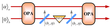
Figure 13: (Color online) Schematic diagram of the photon losses that occur before and after the nonlinear phase. $\eta$ is the transmissivity of the fictitious BS; $b_{v}$ is the vacuum operator.

In our scheme, we consider the QFI of the KSU(1,1) interferometer with the photon losses placed before or after the Kerr nonlinear phase shift in $b$ arm, as shown in Fig. 13. The corresponding Kraus operator $\hat{\Pi}_{l}\left(\phi\right)$ including the nonlinear phase can be written as the general form

$$\hat{\Pi}_{l}\left(\phi\right)=\sqrt{\frac{\left(1-\eta\right)^{l}}{l!}}e^{i\phi[(\hat{b}^{\dagger}\hat{b})^{2}-2\mu_{1}\hat{b}^{\dagger}\hat{b}l-\mu_{2}l^{2}]}\eta^{\frac{\hat{n}}{2}}\hat{b}^{l},$$ (31)

where $\eta$ denotes the strength of the photon loss. $\eta=0$ and $\eta=1$ describe the complete absorption and lossless cases, respectively. $\mu_{1}$ and $\mu_{2}$ are two variational parameters with $\mu_{1}=\mu_{2}=0$ and $\mu_{1}=\mu_{2}=-1$ corresponding to the photon losses occurring before and after the Kerr nonlinear phase shift, respectively.

To derive Eq. (27) using Eq. (31), we shall appeal to the technique of integration within an ordered product of operators (IWOP) 69 to derive the operator identity [see Appendix D], i.e.,

$$\eta^{\hat{n}}\hat{n}^{q}=\colon\left.\frac{\partial^{q}}{\partial x^{q}}e^{\left(\eta e^{x}-1\right)\hat{b}^{\dagger}\hat{b}}\right|_{x=0}\colon,$$ (32)

where $:\cdot:$ indicates the symbol of the normal ordering form, which further leads to the formula [see Appendix D]

$$\sum_{l=0}^{\infty}\frac{\left(1-\eta\right)^{l}}{l!}l^{p}\hat{b}^{\dagger l}\eta^{\hat{n}}\hat{n}^{q}\hat{b}^{l}$$

$$=D_{q,p}\left[\eta e^{x}+\left(1-\eta\right)e^{y}\right]^{\hat{b}^{\dagger}\hat{b}},$$ (33)

with $D_{q,p}=\frac{\partial^{q+p}}{\partial x^{q}\partial y^{p}}\left[\cdot\right]_{|x=y=0}$ being a partial differential operator.

Using Eq. (33) and the following transformation relations

$$e^{\lambda\hat{b}^{\dagger}\hat{b}}\hat{b}^{l}e^{-\lambda\hat{b}^{\dagger}\hat{b}} =e^{-\lambda l}\hat{b}^{l},$$

$$e^{\lambda(\hat{b}^{\dagger}\hat{b})^{2}}\hat{b}^{l}e^{-\lambda(\hat{b}^{\dagger}\hat{b})^{2}} =e^{\lambda l^{2}}\hat{b}^{l}e^{-2\lambda l\hat{b}^{\dagger}\hat{b}},$$ (34)

the upper bound of the QFI $C_{Q}\left[\left|\psi_{S}\right\rangle,\hat{\Pi}_{l}\left(\phi\right)\right]$ can be calculated as [see Appendix E]

$$C_{Q}\left[\left|\psi_{S}\right\rangle,\hat{\Pi}_{l}\left(\phi\right)\right]$$

$$=4(W_{1}^{2}\left\langle\Delta^{2}\hat{n}^{2}\right\rangle-W_{2}\left\langle\hat{n}^{3}\right\rangle+W_{3}\left\langle\hat{n}^{2}\right\rangle$$

$$-W_{4}\left\langle\hat{n}\right\rangle-W_{5}\left\langle\hat{n}^{2}\right\rangle\left\langle\hat{n}\right\rangle-W_{6}\left\langle\hat{n}\right\rangle^{2}),$$ (35)

where $\left\langle\cdot\right\rangle$ and $\left\langle\Delta^{2}\cdot\right\rangle$ are, respectively, the average and variance under the state $\left|\psi_{S}\right\rangle,$ where $\left|\psi_{S}\right\rangle=S\left(\xi_{1}\right)\left|\psi_{in}\right\rangle$ is the state vector after the first OPA. $W_{j}\left(j=1,2,3,4,5,6\right)$ are given in Appendix E, not shown here for simplicity. In particular, when $C_{Q}\left[\left|\psi_{S}\right\rangle,\hat{\Pi}_{l}\left(\phi\right)\right]$ reaches the minimum value corresponding to the QFI $F_{L}$, the variational parameters $\mu_{1}$ and $\mu_{2}$ are, respectively, given by

$$\mu_{1opt} =\frac{BE-CD}{AD-2\eta B^{2}},$$ (36)

$$\mu_{2opt} =\frac{AE-2\eta BC}{AD-2\eta B^{2}},$$ (37)

where $A,B,C,D$ and $E$ are shown in Appendix E. Upon substituting those optimal results $\mu_{1opt}$ and $\mu_{2opt}$ into $C_{Q},$ the minimum value of $C_{Q}$, i.e., the QFI $F_{L}$ of Kerr nonlinear phase shift in the presence of photon losses, can be derived theoretically.

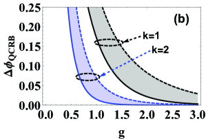
Figure 14: (Color online) The $\Delta\phi_{QCRB}$ as a function of (a) the transmissivity $\eta$ with $g=1$ and $\left|\alpha\right|=1$, (b) the gain factor $g$ with $\left|\alpha\right|=1.$ The black and blue lines correspond to $k=1$,$2$, and the dashed and solid lines to the effects of photon losses and no photon losses, respectively.

Considering a CS and a VS input, here we numerically analyze the QCRB $\Delta\phi_{QCRB}$ which actually is equivalent to the QFI due to the relation in Eq. (15). For fixed parameters with $|\alpha|=1$ and $\theta_{\alpha}=\pi/2,$ the QCRB $\Delta\phi_{QCRB}$ as a function of transmissivity $\eta$ and gain factor $g$ are shown in Fig. 14. For comparison, the linear case with $k=1$ is also plotted here. It is clear that the bound performance of phase sensitivity becomes better and better as the increase of both transmissivity $\eta$ and gain factor $g$ for $k=1,2$ (see dashed lines in Fig. 14 (a) and (b)). The QCRB for $k=2$ always outperforms that for $k=1,$ and the gap between them first increase and then decrease as the increase of $\eta$ and $g$. Compared to the ideal cases (solid lines in Fig. 14(b)), it is clear that photon losses present an obvious effect on the QCRB (dashed lines in Fig. 14(b)). However, it is interesting that the gap of QCRB for $k=2$ between ideal and nonideal cases is significantly smaller than that for $k=1$, which are also going to be smaller as the increase of $g$ especially for $k=2$. Again, this implies that the combination of Kerr nonlinear and OPA can further compress the decoherence effect from the environments.

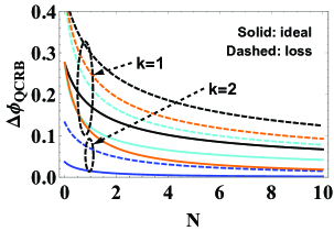
Figure 15: (Color online) The $\Delta\phi_{QCRB}$ as a function of the total average photon number N of input state with $g=1,$ $\eta=0.6.$ The orange- and cyan-dot-dashed lines respectively correspond to a squeezed vacuum state plus a coherent states input and two coherent states with $k=1$, as shown in Ref. 63 . The black and blue lines correspond respectively to $k=1$,2. The dashed and solid lines correspond to the effects of photon losses and no photon losses, respectively.

In addition, under the photon-loss processes (e.g., $\eta=0.6$), we further consider the $\Delta\phi_{QCRB}$ as a function of total average input photon number $N$ for those different input resources above, when given parameter $g=1,$ as shown in Fig. 15. Here the solid lines correspond to the ideal cases for a comparison. It is clearly seen that, compared to other input resources, the $\left|\alpha\right\rangle_{a}\otimes\left|0\right\rangle_{b}$ input presents the worst QCRB in the linear phase shift, with and without photon losses. However, thanks to the introduction of Kerr nonlinear phase, the QCRB for $\left|\alpha\right\rangle_{a}\otimes\left|0\right\rangle_{b}$ input is the best, which is superior to, even in nonideal case, the QCRB in ideal case with other inputs. This means that our scheme with and without photon losses shows an obvious advantage of low-cost input resources to obtain a better QCRB by introducing nonlinear phase instruments in the SU(1,1) interferometer system.

VI Conclusions

In summary, we propose a protocol of second-order nonlinear phase estimation by introducing the Kerr medium into the traditional SU(1,1) interferometer. A kind of simplest inputs, coherent state plus vacuum state, and homodyne detection for one mode are used. Both the phase sensitivity and the QFI or QCRB are analytically derived in both ideal and nonideal scenario by using the CF method and the IWOP technique. It is shown that the increase of both gain factor $g$ and coherent amplitude $\left|\alpha\right|$ is beneficial for improving both the phase sensitivity and the QCRB. Compared to the linear phase estimation, our scheme presents a significantly better performance about both of them, especially around the optimal point $\phi$ $=0$. In particular, for the ideal case, our scheme breaks through both the SQL and the HL, even approaching the SHL, at the large $g$ and $\left|\alpha\right|$ levels. In addition, we consider the effects of the decoherence on the phase sensitivity, from the internal or external photon losses. It is found that the former has a more obvious decoherence than the latter. Even so, our scheme still provides a significant improvement for the performance of phase estimation by homodyne detection, compared to the linear case.

To further show the advantages of our scheme, with and without photon losses, we also consider both the phase sensitivity and the QCRB changing with total average input photon number $N$ for several different input resources, including $\left|\alpha\right\rangle_{a}\otimes\left|0\right\rangle_{b},$ $\left|\alpha\right\rangle_{a}\otimes\left|\beta\right\rangle_{b}$ and $\left|\alpha\right\rangle_{a}\otimes\left|\varsigma,0\right\rangle_{b}$, when given parameters $g=1.$ It is found that the best phase sensitivity can be achieved only using the simplest input $\left|\alpha\right\rangle_{a}\otimes\left|0\right\rangle_{b}$ in the proposed KSU(1,1) interferometer, which is significantly superior to those inputs in the traditional SU(1,1) interferometer. This means that, for a simple input with less energy and less resources, both the phase sensitivity and the QCRB can be further improved by introducing Kerr nonlinear phase. These results may have important applications in other quantum information processing.

Appendix A: Proof of the transformation relation

For a completeness, here, we give the proof about the transformation relation, i.e., $\hat{S}^{\dagger}\left(\phi,2\right)\hat{b}^{\dagger}\hat{S}\left(\phi,2\right)=e^{-i\phi}\hat{b}^{\dagger}e^{-i2\phi\hat{b}^{\dagger}\hat{b}}$. It is well known that any operator $\hat{\zeta}$ can be expanded in Fock state space,

$$\hat{\zeta}=\underset{m,n=0}{\overset{\infty}{\sum}}\zeta_{m,n}\left|m\right\rangle\left\langle n\right|,$$ (A1)

where $\zeta_{m,n}=\left\langle m\right|\hat{\zeta}\left|n\right\rangle$ is the matrix element $\hat{\zeta}$ in Fock space.

Thus, if we take

$$\hat{\zeta} =\hat{S}^{\dagger}\left(\phi,2\right)\hat{b}^{\dagger}\hat{S}\left(\phi,2\right)$$

$$=e^{-i\phi\left(\hat{b}^{\dagger}\hat{b}\right)^{2}}\hat{b}^{\dagger}e^{i\phi\left(\hat{b}^{\dagger}\hat{b}\right)^{2}},$$ (A2)

then the matrix element $\zeta_{m,n}$ can be calculated as

$$\zeta_{m,n}=\sqrt{n+1}e^{-i\phi\left(2n+1\right)}\delta_{m,n+1},$$ (A3)

where we have used the $\hat{b}^{\dagger}\hat{b}\left|n\right\rangle=n\left|n\right\rangle$ and $\hat{b}^{\dagger}\left|n\right\rangle=\sqrt{n+1}\left|n+1\right\rangle.$ Substituting Eq. (A3) into Eq.(A1), we can get

$$\hat{\zeta} =\hat{S}^{\dagger}\left(\phi,2\right)\hat{b}^{\dagger}\hat{S}\left(\phi,2\right)$$

$$=\underset{m,n=0}{\overset{\infty}{\sum}}\sqrt{n+1}e^{-i\phi\left(2n+1\right)}\delta_{m,n+1}\left|m\right\rangle\left\langle n\right|$$

$$=\underset{n=0}{\overset{\infty}{\sum}}\sqrt{n+1}e^{-i\phi\left(2n+1\right)}\left|n+1\right\rangle\left\langle n\right|$$

$$=e^{-i\phi}\underset{n=0}{\overset{\infty}{\sum}}e^{-i2n\phi}\sqrt{n+1}\left|n+1\right\rangle\left\langle n\right|$$

$$=e^{-i\phi}\hat{b}^{\dagger}e^{-i2\phi(\hat{b}^{\dagger}\hat{b})}.$$ (A4)

Appendix B: Phase estimation based on homodyne measurement

Combining Eqs. (3) and (5), we can derive the standard deviation $\Delta\hat{X}$ as

$$\Delta\hat{X}=\sqrt{\left|\overline{U}\right|^{2}+\left|\overline{V}\right|^{2}+\overline{O}},$$ (B1)

where we have set

$$\left|\overline{U}\right|^{2}+\left|\overline{V}\right|^{2}=\cosh^{2}2g-\text{Re}\left(e^{i\phi}\overline{I}\right)\sinh^{2}2g,$$ (B2)

and

$$\overline{O}=2\left|\alpha\right|^{2}\left|u\right|^{2}(1-\left|\overline{I}\left(g,\phi\right)\right|^{2})+2\text{Re}\left(Z_{1}+Z_{2}\right),$$ (B3)

with

$$u =-e^{-i\phi}\sinh^{2}g,$$

$$\chi\left(g,\phi\right) =\frac{1}{\cosh^{2}g-e^{i2\phi}\sinh^{2}g},$$

$$\overline{I}\left(g,\phi\right) =\chi^{2}\left(g,\phi\right)\exp\{\left|\alpha\right|^{2}\left[\chi\left(g,\phi\right)-1\right]\},$$

$$Z_{1} =2(\left|\alpha\right|^{2}+\alpha^{\ast 2})u^{\ast}\overline{I}\left(g,\phi\right)$$

$$\times\left[\chi\left(g,\phi\right)-1\right]\cosh^{2}g,$$

$$Z_{2} =\alpha^{2}u^{2}\overline{I}^{\ast}\left(g,2\phi\right)$$

$$\times[e^{-i2\phi}\chi^{\ast}\left(g,2\phi\right)-\overline{I}^{\ast}\left(g,2\phi\right)],$$ (B4)

and the derivative of $\left\langle\hat{X}\right\rangle$

$$\partial\left\langle\hat{X}\right\rangle/\partial\phi=2\text{Re}\left(Z_{3}Z_{4}\right),$$ (B5)

where Re denotes the real part, and

$$Z_{3} =i\alpha^{\ast}u^{\ast}\overline{I}\left(g,\phi\right),$$

$$Z_{4} =1+4e^{i2\phi}\left|u\right|\chi\left(g,\phi\right)$$

$$+2\left|\alpha\right|^{2}e^{i2\phi}\left|u\right|\chi^{2}\left(g,\phi\right).$$ (B6)

Substituting Eqs. (B1) and (B5) into the error propagation formula in Eq. (6), the explicit expression of the phase sensitivity can be derived theoretically. In particular, when $\phi=0,$ we can get $\left|\overline{U}\right|^{2}+\left|\overline{V}\right|^{2}=1$ and $\overline{O}=0.$ Therefore, the standard deviation $\Delta\hat{X}=1.$ Moreover, utilizing the results from Eq. (B5) at the optimal phase point $\phi=0,$ one can find the absolute value of the derivative

$$\text{ \ \ }\left|\partial\left\langle\hat{X}\right\rangle/\partial\phi\right|$$

$$=\sqrt{N_{\alpha}}N_{OPA}\left[1+N_{OPA}\left(N_{\alpha}+2\right)\right]\sin\theta_{\alpha}.$$ (B7)

Then, after taking $\theta_{\alpha}=\frac{\pi}{2}$ leading to $\sin\theta_{\alpha}=1$, we can obtain Eq. (8).

Appendix C: The QFI in ideal case

For pure quantum system, the QFI can be calculated by Eq. (10), where the average value of operator $A_{m}=\hat{b}^{\dagger m}\hat{b}^{m}$ are needed (see Eq. (11)). In order to obtain the QFI, here we use the method of characteristic function (CF). For any two-mode system, the CF is defined as

$$C_{W}\left(z_{1},z_{2}\right)=\mathtt{Tr}\left[\rho_{out}D\left(z_{1}\right)D\left(z_{2}\right)\right],$$ (C1)

where $D\left(z\right)=\exp\left(z\hat{a}^{\dagger}-z^{\ast}\hat{a}\right)$ is the displacement operator and $\rho_{out}=\left|\varphi_{out}\right\rangle\left\langle\varphi_{out}\right|$ is the density operator after the first OPA. Then the expectation value $\bar{A}_{m}=\left\langle\hat{b}^{\dagger m}\hat{b}^{m}\right\rangle$ can be calculated as

$$\bar{A}_{m}=D_{m}C_{N}\left(0,z_{2}\right),$$ (C2)

where $C_{N}\left(0,z_{2}\right)=e^{\frac{1}{2}\left|z_{2}\right|^{2}}C_{W}\left(0,z_{2}\right)$ is the CF corresponding to normal ordering and $D_{m}=\frac{\partial^{2m}}{\partial z_{2}^{m}\partial\left(-z_{2}^{\ast}\right)^{m}}...|_{z_{2}=z_{2}^{\ast}=0}$ is a partial differential operator. Thus one can use Eq. (C2) to calculate the expectation value $\bar{A}_{m}.$ For our scheme, the input state $\left|\psi_{in}\right\rangle=\left|\alpha\right\rangle_{a}\otimes\left|0\right\rangle_{b}.$ After going through the first OPA and the phase shift, the output state is given by $\left|\psi_{\phi}\right\rangle=\hat{S}\left(\phi,k\right)\hat{S}\left(\xi_{1}\right)\left|\psi_{in}\right\rangle$. Here we should note that these average values of $\bar{A}_{m}$ are under the state $\hat{S}\left(\xi_{1}\right)\left|\psi_{in}\right\rangle$. Then one can obtain

$$\bar{A}_{m}=m!(\sinh^{2m}g)L_{m}(-\left|\alpha\right|^{2}),$$ (C3)

where we have utilized the relation between Laguerre polynomials and two-variable Hermit polynomials,

$$L_{m}\left(xy\right)=\frac{\left(-1\right)^{m}}{m!}H_{m,m}\left(x,y\right),$$ (C4)

and the generating function of $H_{m,m}\left(x,y\right)$ is

$$\text{ \ \ }H_{m,m}\left(x,y\right)$$

$$=\frac{\partial^{2m}}{\partial s^{m}\partial t^{m}}\left.\exp\left(-st+sx+ty\right)\right|_{s=t=0}.$$ (C5)

Thus, substituting Eq. (11) and Eq. (C3) into Eq. (10), one can get the explicit expression of the QFI, for the linear phase shift $\left(k=1\right)$ and Kerr nonlinear phase shift $\left(k=2\right),$ respectively,

$$F_{1} =4\left(\bar{A}_{2}+\bar{A}_{1}-\bar{A}_{1}^{2}\right),$$

$$F_{2} =F_{1}+f,$$

$$f=4\left[\bar{A}_{4}+6\left(\bar{A}_{3}+\bar{A}_{2}\right)-\bar{A}_{2}\left(\bar{A}_{2}+2\bar{A}_{1}\right)\right].$$ (C6)

Appendix D: The Proof of Eqs. (32) and (33)

Using the completeness relation of Fock state, one can get

$$\text{ \ \ }\eta^{\hat{n}}\hat{n}^{q}\underset{\lambda=0}{\overset{\infty}{\sum}}\left|\lambda\right\rangle\left\langle\lambda\right|$$

$$=\sum_{\lambda=0}^{\infty}\eta^{\lambda}\lambda^{q}\frac{\hat{b}^{\dagger\lambda}}{\lambda!}\left|0\right\rangle\left\langle 0\right|\hat{b}^{\lambda}$$

$$=:\underset{\lambda=0}{\overset{\infty}{\sum}}\eta^{\lambda}\lambda^{q}\frac{1}{\lambda!}\hat{b}^{\dagger\lambda}e^{-\hat{b}^{\dagger}\hat{b}}\hat{b}^{\lambda}\colon$$

$$=\colon\left.e^{-\hat{b}^{\dagger}\hat{b}}\underset{\lambda=0}{\overset{\infty}{\sum}}\frac{(\eta\hat{b}^{\dagger}\hat{b})^{\lambda}}{\lambda!}\frac{\partial^{q}}{\partial x^{q}}e^{x\lambda}\right|_{x=0}\colon$$

$$=\colon\left.\frac{\partial^{q}}{\partial x^{q}}e^{\left(\eta e^{x}-1\right)\hat{b}^{\dagger}\hat{b}}\right|_{x=0}\colon,$$ (D1)

where we have used the normal ordering form of the vacuum projection operator

$$\left|0\right\rangle\left\langle 0\right|=\colon e^{-\hat{b}^{\dagger}\hat{b}}\colon.$$ (D2)

Then, using Eq. (D1), one can calculate the following sum operator, i.e.,

$$\underset{l=0}{\overset{\infty}{\sum}}\frac{\left(1-\eta\right)^{l}}{l!}l^{p}\hat{b}^{\dagger l}\eta^{\hat{n}}\hat{n}^{q}\hat{b}^{l}$$

$$=\underset{l=0}{\overset{\infty}{\sum}}\frac{\left(1-\eta\right)^{l}}{l!}l^{p}\colon\left.(\hat{b}^{\dagger}\hat{b})^{l}\frac{\partial^{q}}{\partial x^{q}}e^{\left(\eta e^{x}-1\right)\hat{b}^{\dagger}\hat{b}}\right|_{x=0}\colon$$

$$=\colon\left.\underset{l=0}{\overset{\infty}{\sum}}\frac{\left[\left(1-\eta\right)\hat{b}^{\dagger}\hat{b}\right]^{l}}{l!}\frac{\partial^{q+p}}{\partial x^{q}\partial y^{p}}e^{\left(\eta e^{x}-1\right)\hat{b}^{\dagger}\hat{b}+yl}\right|_{x=y=0}\colon$$

$$=\colon\left.\frac{\partial^{q+p}}{\partial x^{q}\partial y^{p}}e^{\left[\eta e^{x}+\left(1-\eta\right)e^{y}-1\right]\hat{b}^{\dagger}\hat{b}}\right|_{x=y=0}\colon$$

$$=\left.\frac{\partial^{q+p}}{\partial x^{q}\partial y^{p}}[\eta e^{x}+\left(1-\eta\right)e^{y}]^{\hat{b}^{\dagger}\hat{b}}\right|_{x=y=0}.$$ (D3)

In the last step, we have used the following operator identity about $e^{\lambda\hat{b}^{\dagger}\hat{b}}$ i.e.,

$$e^{\lambda\hat{b}^{\dagger}\hat{b}}=\colon e^{\left(e^{\lambda}-1\right)\hat{b}^{\dagger}\hat{b}}\colon,$$ (D4)

to remove the symbol of normal ordering.

Appendix E: The specific expression of $C_{Q}$

Using Eqs. (27), (33) and Eqs. (29) and (31), one can get

$$C_{Q} =4(W_{1}^{2}\left\langle\Delta^{2}\hat{n}^{2}\right\rangle-W_{2}\left\langle\hat{n}^{3}\right\rangle+W_{3}\left\langle\hat{n}^{2}\right\rangle$$

$$\text{ \ \ \ }-W_{4}\left\langle\hat{n}\right\rangle-W_{5}\left\langle\hat{n}^{2}\right\rangle\left\langle\hat{n}\right\rangle-W_{6}\left\langle\hat{n}\right\rangle^{2}),$$ (E1)

where we have set

$$W_{1} =w_{1}\eta^{2}-2w_{2}\eta-\mu_{2},$$

$$W_{2} =2\eta\left(3w_{1}^{2}\eta^{3}-3w_{3}\eta^{2}-w_{4}\eta+w_{5}\right),$$

$$W_{3} =\eta\left(11w_{1}^{2}\eta^{3}-2w_{6}\eta^{2}+w_{7}\eta-4w_{1}w_{2}\right),$$

$$W_{4} =\eta\left(6\eta^{3}-12\eta^{2}+7\eta-1\right)w_{1}^{2},$$

$$W_{5} =2\eta\left(1-\eta\right)w_{1}W_{1},$$

$$W_{6} =\eta^{2}\left(1-\eta\right)^{2}w_{1}^{2},$$ (E2)

as well as

$$w_{1} =1+2\mu_{1}-\mu_{2},$$

$$w_{2} =\mu_{1}-\mu_{2},$$

$$w_{3} =1+2\left(3\mu_{1}-2\mu_{2}\right)$$

$$\text{ \ \ \ \ }+\left(2\mu_{1}-\mu_{2}\right)\left(4\mu_{1}-3\mu_{2}\right),$$

$$w_{4} =7\mu_{2}-6\mu_{1}+24\mu_{1}\mu_{2}-14\mu_{1}^{2}-9\mu_{2}^{2},$$

$$w_{5} =\mu_{2}w_{1}-2w_{2}^{2},$$

$$w_{6} =9+40\mu_{1}-22\mu_{2}+44\mu_{1}^{2}-48\mu_{1}\mu_{2}+13\mu_{2}^{2},$$

$$w_{7} =7+40\mu_{1}-26\mu_{2}+52\mu_{1}^{2}-64\mu_{1}\mu_{2}+19\mu_{2}^{2}.$$ (E3)

In particular, when $\mu_{1}=\mu_{2}=-1$, one can obtain the expected result, i.e.,

$$F_{L_{2}}\leqslant C_{Q}=4\left\langle\Delta^{2}\hat{n}^{2}\right\rangle.$$ (E4)

While for $\mu_{1}=\mu_{2}=0,$ corresponding to the photon losses before the Kerr nonlinear phase shift, one can get the upper bound, i.e.,

$$F_{L_{2}} \leqslant C_{Q}=4[\eta^{4}\left\langle\Delta^{2}\hat{n}^{2}\right\rangle+6\eta^{3}\left(1-\eta\right)\left\langle\hat{n}^{3}\right\rangle$$

$$\text{ \ \ \ }+\eta^{2}\left(11\eta^{2}-18\eta+7\right)\left\langle\hat{n}^{2}\right\rangle$$

$$\text{ \ \ \ }-\eta\left(6\eta^{3}-12\eta^{2}+7\eta-1\right)\left\langle\hat{n}\right\rangle$$

$$\text{ \ \ \ }-2\eta^{3}\left(1-\eta\right)\left\langle\hat{n}^{2}\right\rangle\left\langle\hat{n}\right\rangle$$

$$\text{ \ \ \ }-\eta^{2}\left(1-\eta\right)^{2}\left\langle\hat{n}\right\rangle^{2}],$$ (E5)

as expected.

In order to minimize $C_{Q},$ one can take $\partial C_{Q}/\partial\mu_{1}=\partial C_{Q}/\partial\mu_{2}=0$ for this purpose. Using Eqs. (E1)-(E3), it is not difficult to obtain two optimization parameters $\mu_{1opt}$ and $\mu_{2opt}$, which are, respectively, given by

$$\mu_{1opt}=\frac{BE-CD}{AD-2\eta B^{2}},\mu_{2opt}=\frac{AE-2\eta BC}{AD-2\eta B^{2}},$$ (E6)

where we have set $A=2B_{1}H,$ $B=B_{2}H,$ $C=B_{3}H,$ $D=B_{4}H,$ and $E=\eta B_{5}H.$ Here the column matrix $H$ and row matrix $B_{j}\left(j=1,2,3,4,5\right)$ are defined as the following

$$H =(\left\langle\Delta^{2}\hat{n}^{2}\right\rangle,\left\langle\hat{n}^{3}\right\rangle,\left\langle\hat{n}^{2}\right\rangle,$$

$$\text{ \ \ \ }\left\langle\hat{n}\right\rangle,\left\langle\hat{n}^{2}\right\rangle\left\langle\hat{n}\right\rangle,\left\langle\hat{n}\right\rangle^{2})^{T},$$

$$A_{1} =\eta-1,$$

$$A_{2} =6\eta^{2}-6\eta+1,$$

$$A_{3} =11\eta^{2}-11\eta+2,$$

$$A_{4} =2\eta-1,$$

$$B_{1} =\left(\eta A_{1},-A_{2},A_{3},-A_{2},2\eta A_{1},-\eta A_{1}\right),$$

$$B_{2} =(A_{1}^{2},-3A_{1}A_{4},A_{3}-A_{4},$$

$$\text{ \ \ \ }-A_{2},A_{1}A_{4},-\eta A_{1}),$$

$$B_{3} =\left(\eta^{2},-3\eta A_{4},A_{3}+A_{4},-A_{2},\eta A_{4},-\eta A_{1}\right),$$

$$B_{4} =\eta(\eta^{-1}A_{1}^{3},-6A_{1}^{2},A_{3}-2A_{4},$$

$$\text{ \ \ \ }-A_{2},2A_{1}^{2},-\eta A_{1}),$$

$$B_{5} =\left(\eta A_{1},-A_{2},A_{3},-A_{2},\eta^{2}+A_{1}^{2},-\eta A_{1}\right),$$ (E7)

where the average value $\left\langle\cdot\right\rangle$ is in the state after the first OPA. Here we should note that, only $H$ are dependent on the input state, and the other quantities (such as $A_{j},B_{j}$) are independent of the input state. If $C_{Q}$ can take the minimum value, then it is also the QFI $F_{L_{2}}$ of Kerr nonlinear phase shift in the presence of photon losses. In our scheme, if we choose the states $\left|\psi_{in}\right\rangle=\left|\alpha\right\rangle_{a}\otimes\left|0\right\rangle_{b}$ as the inputs of the KSU(1,1) interferometer, then the states after the first OPA is $\hat{S}\left(\xi_{1}\right)\left|\psi_{in}\right\rangle$. Thus the column matrix $H$ can be calculated as

$$H =[\frac{F_{2}}{4},\left(\bar{A}_{3}+3\bar{A}_{2}+\bar{A}_{1}\right),$$

$$\text{ \ \ \ }\left(\bar{A}_{2}+\bar{A}_{1}\right),\bar{A}_{1},\bar{A}_{1}\left(\bar{A}_{2}+\bar{A}_{1}\right),\bar{A}_{1}^{2}]^{T},$$ (E8)

where $F_{2}$ is lossless result in Eq. (12) and $\bar{A}_{j}\left(j=1,2,3\right)$ and $W_{l}(l=1\sim 6)$ can be obtained from Eqs. (C3) and (E2), respectively.

Further substituting Eq. (E8) and Eq. (E6) into Eq. (E1), the upper bound to the QFI $C_{Q}\left(\left|\alpha\right\rangle_{a}\otimes\left|0\right\rangle_{b}\right)$ in our scheme can be obtained as

$$\text{ \ \ \ }C_{Q}\left(\left|\alpha\right\rangle_{a}\otimes\left|0\right\rangle_{b}\right)$$

$$=W_{1}^{2}F_{2}-4[W_{2}\left(\bar{A}_{3}+3\bar{A}_{2}+\bar{A}_{1}\right)$$

$$\text{ \ \ \ }-W_{3}\left(\bar{A}_{2}+\bar{A}_{1}\right)+W_{4}\bar{A}_{1}$$

$$\text{ \ \ \ }+W_{5}\bar{A}_{1}\left(\bar{A}_{2}+\bar{A}_{1}\right)+W_{6}\bar{A}_{1}^{2}],$$ (E9)

which is just the analytical expression of the QFI. In $W_{l}(l=1\sim 6)$, the variational parameters $\mu_{1}$ and $\mu_{2}$ should be replaced, respectively, by

$$\mu_{1opt}\left(\left|\alpha\right\rangle_{a}\otimes\left|0\right\rangle_{b}\right) =\frac{BE-CD}{AD-2\eta B^{2}},$$

$$\mu_{2opt}\left(\left|\alpha\right\rangle_{a}\otimes\left|0\right\rangle_{b}\right) =\frac{AE-2\eta BC}{AD-2\eta B^{2}},$$ (E10)

where $A=2B_{1}H,$ $B=B_{2}H,$ $C=B_{3}H,$ $D=B_{4}H,$ and $E=\eta B_{5}H$ with the column matrix $H$ is shown in Eq. (E8).

In addition, for a comparison between the linear phase shift and the nonlinear one (our scheme), here we give the QFI with the linear phase shift in the presence of photon losses, for several different input states, including $\left|\alpha\right\rangle_{a}\otimes\left|0\right\rangle_{b}$ (CS&VS), $\left|\alpha\right\rangle_{a}\otimes\left|\beta\right\rangle_{b}$ (CS&CS) and $\left|\alpha\right\rangle_{a}\otimes\left|\varsigma,0\right\rangle_{b}$ (CS&SVS). In a similar way to derive Eq. (E9), for these states above together with the linear phase shift, the QFI $F_{L_{1}}$ can be calculated as 68

$$\text{ \ \ }F_{L_{1}\left(CS\&VS\right)}$$

$$=\frac{4\eta F_{1}\bar{A}_{1}}{\left(1-\eta\right)F_{1}+4\eta\bar{A}_{1}},$$

$$\text{ \ \ }F_{L_{1}\left(CS\&CS\right)}$$

$$=\frac{4\eta F_{\left(CS\&CS\right)}\left\langle\hat{n}\right\rangle_{\left(CS\&CS\right)}}{\left(1-\eta\right)F_{\left(CS\&CS\right)}+4\eta\left\langle\hat{n}\right\rangle_{\left(CS\&CS\right)}},$$

$$\text{ \ \ }F_{L_{1}\left(CS\&SVS\right)}$$

$$=\frac{4\eta F_{\left(CS\&SVS\right)}\left\langle\hat{n}\right\rangle_{\left(CS\&SVS\right)}}{\left(1-\eta\right)F_{\left(CS\&SVS\right)}+4\eta\left\langle\hat{n}\right\rangle_{\left(CS\&SVS\right)}},$$ (E11)

where $\left\langle\hat{n}\right\rangle_{\left(CS\&CS\right)}$ and $\left\langle\hat{n}\right\rangle_{\left(CS\&SVS\right)}$ are given by

$$\text{ \ \ }\left\langle\hat{n}\right\rangle_{\left(CS\&CS\right)}$$

$$=\left(\left|\alpha\right|\sinh g+\left|\beta\right|\cosh g\right)^{2}+\sinh^{2}g,$$

$$\text{ \ \ }\left\langle\hat{n}\right\rangle_{\left(CS\&SVS\right)}$$

$$=\left(\left|\alpha\right|^{2}+1\right)\sinh^{2}g+\cosh^{2}g\left(\sinh^{2}r\right),$$ (E12)

and $F_{\left(CS\&CS\right)}$ and $F_{\left(CS\&SVS\right)}$ are the lossless results which can be seen from Ref. 63 , i.e.,

$$\text{ \ \ }F_{\left(CS\&CS\right)}$$

$$=(\left|\alpha\right|^{2}+\left|\beta\right|^{2})\cosh 4g+\sinh^{2}(2g)$$

$$\text{ \ \ }+2\left|\alpha\right|\left|\beta\right|\sinh 4g+\left|\alpha\right|^{2}+\left|\beta\right|^{2}$$

$$\text{ \ \ }-2\left(\left|\alpha\right|^{2}-\left|\beta\right|^{2}\right)\cosh 2g,$$ (E13)

$$\text{ \ \ }F_{\left(CS\&SVS\right)}$$

$$=\cosh^{2}\left(2g\right)[\frac{1}{2}\sinh^{2}\left(2r\right)+\left|\alpha\right|^{2}]$$

$$\text{ \ \ }+\sinh^{2}(2g)(\left|\alpha\right|^{2}e^{2r}+\cosh^{2}r)$$

$$\text{ \ \ }+\left|\alpha\right|^{2}\left(1-2\cosh 2g\right)$$

$$\text{ \ \ }+\frac{1}{4}(\cosh 4r-1)(2\cosh 2g+1).$$ (E14)

References

• (1) C. Lee, J. Huang, H. Deng, H. Dai, and J. Xu, Nonlinear quantum interferometry with Bose condensed atoms, Front. Phys. 7, 109 (2012)
• (2) J. Estève, C. Gross, A. Weller, S. Giovanazzi, and M. K. Oberthaler, Squeezing and entanglement in a Bose–Einstein condensate, Nature (London) 455, 1216 (2008).
• (3) A. C. J. Wade, J. F. Sherson, and K. Molmer, Squeezing and Entanglement of Density Oscillations in a Bose-Einstein Condensate, Phys. Rev. Lett. 115, 060401 (2015).
• (4) E. Oelker, L. Barsotti, S. Dwyer, D. Sigg, and N. Mavalvala, Squeezed light for advanced gravitational wave detectors and beyond, Opt. Express 22, 21106 (2014).
• (5) H. Vahlbruch, D. Wilken, M. Mehmet, and B. Willke, Laser Power Stabilization beyond the Shot Noise Limit Using Squeezed Light, Phys. Rev. Lett. 121, 173601 (2018).
• (6) M. Tsang, Quantum Imaging beyond the Diffraction Limit by Optical Centroid Measurements, Phys. Rev. Lett. 102, 253601 (2009).
• (7) N. Bornman, S. Prabhakar, A. Vallés, J. Leach, and A. Forbes, Ghost imaging with engineered quantum states by Hong–Ou–Mandel interference, New J. Phys. 21, 073044 (2019).
• (8) S. D. Huver, C. F. Wildfeuer, J. P. Dowling, Entangled Fock states for robust quantum optical metrology, imaging, and sensing, Phys. Rev. A 78, 063828 (2008).
• (9) J. D. Zhang, Z. J. Zhang, L. Z. Cen, J. Y. Hu, and Y. Zhao, Nonlinear phase estimation: Parity measurement approaches the quantum Cramér-Rao bound for coherent states, Phys. Rev. A 99, 022106 (2019).
• (10) H. Liang, Y. Su, X. Xiao, Y. Che, B. C. Sanders, and X. G. Wang, Criticality in two-mode interferometers, Phys. Rev. A 102, 013722 (2020).
• (11) S. Ataman, Optimal Mach-Zehnder phase sensitivity with Gaussian states, Phys. Rev. A 100, 063821 (2019).
• (12) C. P. Wei, Z. M. Wu, C. Z. Deng, and L. Y. Hu, Phase sensitivity of a three-mode nonlinear interferometer, Opt. Commun. 452, 189-194 (2019).
• (13) J. Joo, W. J. Munro, T. P. Spiller, Quantum metrology with entangled coherent states, Phys. Rev. Lett. 107, 083601 (2011).
• (14) R. Birrittella, C. C. Gerry, Quantum optical interferometry via the mixing of coherent and photon-subtracted squeezed vacuum states of light, J. Opt. Soc. Am. B 31, 586–593 (2014).
• (15) J. P. Dowling, Quantum optical metrology–the lowdown on high-N00N states, Contemp. Phys. 49, 125–143 (2008).
• (16) L. Y. Hu, C. P. Wei, J. H. Huang, and C. J. Liu, Quantum metrology with Fock and even coherent states: Parity detection approaches to the Heisenberg limit, Opt. Commun. 323, 68–76 (2014).
• (17) J. Kong, Z. Y. Ou, and W. P. Zhang, Phase-measurement sensitivity beyond the standard quantum limit in an interferometer consisting of a parametric amplifier and a beam splitter, Phys. Rev. A 87, 023825 (2013).
• (18) Z. Y. Ou, Enhancement of the phase-measurement sensitivity beyond the standard quantum limit by a nonlinear interferometer, Phys. Rev. A 85, 023815 (2012).
• (19) S. H. Tan, Y. Y. Gao, H. de Guise, and B. C. Sanders, SU(3) Quantum Interferometry with Single-Photon Input Pulses, Phys. Rev. Lett. 110, 113603 (2013).
• (20) B. Yurke, S. L. McCall, and J. R. Klauder, SU(2) and SU(1,1) interferometers, Phys. Rev. A 33, 4033 (1986)
• (21) H. M. Ma, D. Li, C. H. Yuan, L. Q. Chen, Z. Y. Ou, and W. P. Zhang, SU(1,1)-type light-atom-correlated interferometer, Phys. Rev. A 92, 023847 (2015).
• (22) E. Distante, M. Ježek, and U. L. Andersen, Deterministic Superresolution with Coherent States at the Shot Noise Limit, Phys. Rev. Lett. 111, 033603 (2013).
• (23) X. M. Feng, G. R. Jin, and W. Yang, Quantum interferometry with binary-outcome measurements in the presence of phase diffusion, Phys. Rev. A 90, 013807 (2014).
• (24) R. A. Campos, C. C. Gerry, and A. Benmoussa, Optical interferometry at the Heisenberg limit with twin Fock states and parity measurements, Phys. Rev. A 68, 023810 (2003).
• (25) Y. Israel, S. Rosen, and Y. Silberberg, Supersensitive Polarization Microscopy Using NOON States of Light, Phys. Rev. Lett. 112, 103604 (2014).
• (26) C. M. Caves, Quantum-mechanical noise in an interferometer, Phys. Rev. D 23, 1693 (1981).
• (27) P. M. Anisimov, G. M. Raterman, A. Chiruvelli, W. N. Plick, S. D. Huver, H. Lee, and J. P. Dowling, Quantum Metrology with Two-Mode Squeezed Vacuum: Parity Detection Beats the Heisenberg Limit, Phys. Rev. Lett. 104, 103602 (2010).
• (28) J. Fiurášek, Conditional generation of N-photon entangled states of light, Phys. Rev. A 65, 053818 (2002).
• (29) A. Ourjoumtsev, H. Jeong, R. Tualle-Brouri, and P. Grangier, Generation of optical ‘Schröinger cats’ from photon number states, Nature (London) 448, 784 (2007).
• (30) T. Ono and H. F. Hofmann, Effects of photon losses on phase estimation near the Heisenberg limit using coherent light and squeezed vacuum, Phys. Rev. A 81, 033819 (2010).
• (31) D. Li, C. H. Yuan, Z. Y. Ou, W. P. Zhang, The phase sensitivity of an SU(1,1) interferometer with coherent and squeezed-vacuum light, New J. Phys. 16, 073020 (2014).
• (32) X. Y. Hu, C. P. Wei, Y. F. Yu, Z. M. Zhang, Enhanced phase sensitivity of an SU(1,1) interferometer with displaced squeezed vacuum light, Front. Phys. 11, 114203 (2016).
• (33) W. N. Plick, J. P. Dowling, G. S. Agarwal, Coherent-light-boosted, sub-shot noise, quantum interferometry, New J. Phys. 12, 083014 (2010).
• (34) L. L. Guo, Y. F. Yu, Z. M. Zhang, Improving the phase sensitivity of an SU(1,1) interferometer with photon-added squeezed vacuum light, Opt. Express 26, 29099 (2018).
• (35) D. Li, B. T. Gard, Y. Gao, C. H. Yuan, W. P. Zhang, H. Lee, J. P. Dowling, Phase sensitivity at the Heisenberg limit in an SU(1,1) interferometer via parity detection, Phys. Rev. A 94, 063840 (2016).
• (36) S. Adhikari, N. Bhusal, C. You, H. Lee, and J. P. Dowling, Phase estimation in an SU(1,1) interferometer with displaced squeezed states, Opt. Express 1, 438 (2018).
• (37) C. Sparaciari, S. Olivares, M. G. A. Paris, Gaussian-state interferometry with passive and active elements, Phys. Rev. A 93, 023810 (2016).
• (38) F. Hudelist, J. Kong, C. J. Liu, J. T. Jing, Z. Y. Ou, and W. P. Zhang, Quantum metrology with parametric amplifier-based photon correlation interferometers, Nat. Commun. 5, 3049 (2014).
• (39) G. F. Jiao, K. Y. Zhang, L. Q. Chen, W. P. Zhang, and C. H. Yuan, Nonlinear phase estimation enhanced by an actively correlated Mach-Zehnder interferometer, Phys. Rev. A 102, 033520 (2020).
• (40) O. Seth, X. F. Li, H. N. Xiong, J. Y. Luo and Y. X. Huang, Improving the phase sensitivity of an SU(1,1) interferometer via a nonlinear phase encoding, J. Phys. B: At. Mol. Opt. Phys. 53, 205503 (2020).
• (41) S. K. Chang, C. P. Wei, H. Zhang, Y. Xia, W. Ye, and L. Y. Hu, Enhanced phase sensitivity with a nonconventional interferometer and nonlinear phase shifter, Phys. Lett. A 384, 126755 (2020).
• (42) C. P. Wei, Z. M. Zhang, Improving the phase sensitivity of a Mach–Zehnder interferometer via a nonlinear phase shifter, J. Mod. Opt. 64, 743–749 (2017).
• (43) Z. Tong, C. Lundström, P. A. Andrekson, C. J. Mckinstrie, M. Karlsson, D. J. Blessing, E. Tipsuwannakul, B. J. Puttnam, H. Toda, and L. Grüernielsen, Towards ultrasensitive optical links enabled by low-noise phase-sensitive amplifiers, Nat. Photonics 5, 430 (2011).
• (44) N. V. Corzo, A. M. Marino, K. M. Jones, and P. D. Lett, Noiseless Optical Amplifier Operating on Hundreds of Spatial Modes, Phys. Rev. Lett. 109, 043602 (2012).
• (45) J. Joo, K. Park, H. Jeong, W. J. Munro, K. Nemoto, T. P. Spiller, Quantum metrology for nonlinear phase shifts with entangled coherent states, Phys. Rev. A 86 043828 (2012).
• (46) L. Dong, J. X. Wang, Q. Y. Li, H. Z. Shen, H. K. Dong, X. M. Xiu, Y. J. Gao, and C. H. Oh, Nearly deterministic preparation of the perfect W state with weak cross-Kerr nonlinearities, Phys. Rev. A 93, 012308 (2016).
• (47) S. Ataman, Phase sensitivity of a Mach-Zehnder interferometer with single-intensity and difference-intensity detection, Phys. Rev. A 98, 043856 (2018).
• (48) X. Xiao, H. B. Liang, G. L. Li, and X. G. Wang, Enhancement of Sensitivity by Initial Phase Matching in SU(1,1) Interferometers, Commun. Theor. Phys. 71, 37 (2019).
• (49) X. X. Jing, J. Liu, W. Zhong, and X. G. Wang, Quantum Fisher Information of Entangled Coherent States in a Lossy Mach-Zehnder Interferometer, Commun. Theor. Phys. 61, 115 (2014).
• (50) H. Zhang, W. Ye, C. P. Wei, Y. Xia, S. K. Chang, Z. Y. Liao, and L. Y. Hu, Improved phase sensitivity in a quantum optical interferometer based on multiphoton catalytic two-mode squeezed vacuum states, Phys. Rev. A 103, 013705 (2021).
• (51) K. P. Seshadreesan, S. Kim, J. P. Dowling, and H. Lee, Phase estimation at the quantum Cramér-Rao bound via parity detection, Phys. Rev. A 87, 043833 (2013).
• (52) W. Ye, H. Zhong, Q. Liao, D. Huang, L. Y. Hu, Y. Guo, Improvement of self-referenced continuous-variable quantum key distribution with quantum photon catalysis, Opt. Express 27, 17186 (2019).
• (53) L. Y. Hu, M. Al-amri, Z. Y. Liao, and M. S. Zubairy, Continuous-variable quantum key distribution with non-Gaussian operations, 102, 012608 (2020).
• (54) Y. Guo, W. Ye, H. Zhong, Q. Liao, Continuous-variable quantum key distribution with non-Gaussian quantum catalysis, Phys. Rev. A 99, 032327 (2019).
• (55) S. L. Braunstein, P. V. Loock, Quantum information with continuous variables, Rev. Mod. Phys. 77, 513 (2005).
• (56) W. Ye, Y. Guo, Y. Xia, H. Zhong, H. Zhang, J. Z. Ding, L. Y. Hu, Discrete modulation continuous-variable quantum key distribution based on quantum catalysis, Acta Phys. Sin. 69, 060301 (2020).
• (57) J. Cheng, Quantum metrology for simultaneously estimating the linear and nonlinear phase shifts, Phys. Rev. A 90, 063838 (2014).
• (58) A. Luis, Quantum limits, nonseparable transformations, and nonlinear optics, Phys. Rev. A 76, 035801 (2007).
• (59) S. Boixo, A. Datta, S. T. Flammia, A. Shaji, E. Bagan, and C. M. Caves, Quantum-limited metrology with product states, Phys. Rev. A 77, 012317 (2008).
• (60) S. Boixo, A. Datta, M. J. Davis, S. T. Flammia, A. Shaji, and C. M. Caves, Quantum Metrology: Dynamics versus Entanglement, Phys. Rev. Lett. 101, 040403 (2008).
• (61) M. Napolitano and M. W. Mitchell, Nonlinear metrology with a quantum interface, New J. Phys. 12, 093016 (2010).
• (62) M. Zwierz, C. A. Pérez-Delgado, and P. Kok, General Optimality of the Heisenberg Limit for Quantum Metrology, Phys. Rev. Lett. 105, 180402 (2010).
• (63) Q. K. Gong, D. Li, C. H. Yuan, Z. Y. Qu, and W. P. Zhang, Phase estimation of phase shifts in two arms for an SU(1,1) interferometer with coherent and squeezed vacuum states, Chin. Phys. B 26, 094205 (2017).
• (64) D. Li, C. H. Yuan, Y. Yao, W. Jiang, M. Li, W. P. Zhang, Effects of loss on the phase sensitivity with parity detection in an SU(1,1) interferometer, J. Opt. Soc. Am. B 35, 5 (2018).
• (65) R. Demkowicz-Dobrzański, M. Jarzyna, and J. Kołodyński, Quantum limits in optical interferometry, Prog. Opt. 60, 345 (2015).
• (66) S. Knysh, V. N. Smelyanskiy, and G. A. Durkin, Scaling laws for precision in quantum interferometry and the bifurcation landscape of the optimal state, Phys. Rev. A 83, 021804(R) (2011).
• (67) J. Liu, X. X. J, and X. G. Wang, Phase-matching condition for enhancement of phase sensitivity in quantum metrology, Phys. Rev. A 88, 042316 (2013).
• (68) B. M. Escher, R. L. de Matos Filho, and L. Davidovich, General framework for estimating the ultimate precision limit in noisy quantum-enhanced metrology, Nat. Phys. 7, 406 (2011).
• (69) H. Y. Fan, H. L. Lu, and Y. Fan, Newton–Leibniz integration for ket–bra operators in quantum mechanics and derivation of entangled state representations, Ann. Phys. 321, 480 (2006).