Multi-particle quantum walks and Fisher information in one-dimensional lattices

Abstract

Recent experiments on quantum walks (QWs) demonstrated a full control over the statistics-dependent walks of single and two particles in one-dimensional (1D) lattices. However little is known about the general characterization of QWs at the many-body level. Here we rigorously study QWs, Bloch oscillations and quantum Fisher informations (FIs) for three indistinguishable bosons and fermions in 1D lattices using time-evolving block decimation algorithm and many-body perturbation theory. We show that such strongly correlated QWs not only give rise to statistics-and-interaction-dependent ballistic transports of scattering states and of two- and three-body bound states, but also allow a quantum enhanced precision measurement of the gravitational force. In contrast to the QWs of the fermions, the QWs of three bosons exhibit strongly correlated Bloch oscillations, which present a surprising time scaling $t^{3}$ of FI below a characteristic time $t_{0}$ and saturate to the fundamental limit of $t^{2}$ for $t>t_{0}$.

Quantum walks (QW) Aharonov1 ; Kempe1 , the quantum counterpart of the classical random walks, are characterized by a fast ballistic spreading with wave fronts expanding linearly in time. Owing to their non-classical features, they have potential applications in quantum algorithms Ambainis1 , quantum computing Childs1 , quantum information Andraca1 ; Zatelli:2020 , quantum simulation Asboth1 and quantum biology Lloyd1 . QWs have been experimentally implemented in a variety of quantum systems Wang1 , and recently found in detecting topological states Kitagawa1 ; Kraus1 ; Ramasesh1 , discrete-time QWs Cedzich1 ; Arnault1 ; Destri1 ; Bisio1 , and bound states of magnons Ahlbrecht1 ; Fukuhara1 .

Up to now, most previous works focused on the one and two-particle QWs in 1D lattices. Preliminary experiments studied the QWs of single and two particles by using either neutral atoms Karski1 , ions Schmitz1 , photons Schreiber1 , spin impurities Fukuhara1 ; Fukuhara2 , or nuclear-magnetic-resonance systems Du1 . Walkers of two non-interacting particles can develop non-trivial correlations due to the Hanbury-Brown-Twiss interference Peruzzo1 ; Mayer1 ; Hillery1 ; Sansoni1 ; Solntsev1 ; Lahini1 ; Brown1 . Bosonic (fermionic) walkers result in an emergence of bunching (anti-bunching) in density-density correlations Omar1 ; Benedetti1 ; Qin1 ; Preiss1 , and anyons are in between Wang2 ; Lau:2020 . Moreover, the interplay between quantum statistics and interaction of two particles Iyer:2013 ; Preiss1 ; Ganahl1 ; Krapivsky1 ; Wiater1 ; Qin1 ; Siloi:2017 ; Beggi:2018 ; Sarkar:2020 , and of two and three flipped spins in a Heisenberg Chain Liu1 , leads to a richer dynamics of quantum co-walking.

On the other hand, a quantum particle in a tilted periodic potential may undergo Bloch oscillation (BO), which has been demonstrated via ultracold atoms Preiss1 ; Geiger1 . The BO frequency is proportional to the tilting force. This can be employed to measure the gravitational force Ferrari1 ; Tarallo1 , the magnetic field gradient LiuWJ , the Zak phase in topological Bloch bands Atala1 and the Casimir-Polder force Carusotto1 . Quantum Fisher Information (FI), which provides a lower limit to the Cramér-Rao bound, plays a central role in quantum precision measurements Helstrom:1976 ; Pezze1 ; Liu2 . However, the question how to create many-body entanglement to improve measurements precision via BOs and how to use the FIs to quantify the precision limit for the gravitational force still remains open and challenging.

In this Letter, we study nonequilibrium dynamics of three fermions and bosons in 1D lattices and explore its metrological application in precision measurement of gravitational force. Continuous-time QWs, strongly correlated BOs, the band structure, time-evolutions of density distributions and density-density correlations for the systems are thoroughly studied through both numerical and analytical methods. The FIs of such QWs show a promising capability of quantum-enhanced precision measurement of weak forces in the walks of three-boson bound states.

The Model.– We consider three indistinguishable particles moving on 1D lattices governed by the Hamiltonian:

$$\hat{H}=-J\sum_{j=-M}^{M-1}(a^{\dagger}_{j}a_{j+1}+\mathrm{H.c})+V\sum_{j=-M}^{M-1}\hat{n}_{j}\hat{n}_{j+1}.$$ (1)

Here $a^{\dagger}_{j}$ ($a_{j}$) creates (annihilates) a particle at the $j$-th site, and $\hat{n}_{j}=a^{\dagger}_{j}a_{j}$ is the particle number operator. The total number of lattice sites $L=2M$. $J$ is the nearest-neighbour hopping and set the unit of energy ($J=1$). $V$ is the nearest-neighbour interaction. Hamiltonians of this kind (1) can be realized with ultracold atoms Preiss1 ; Sun:2020e ; Yang:2020e . Here we study two types of particles: bosons and fermions. The fermonic model is equivalent to the exactly solvable XXZ Heisenberg chain YY:1966 ; Takahashi1 which is also equivalent to the hard-core bosonic model Jordan1 . The QW of two and three particles of the XXZ model was found in Liu1 and an experimental realization via ultracold two-level atoms in deep optical lattices was given in Lee2004 ; Qin1 ; LiuWJ .

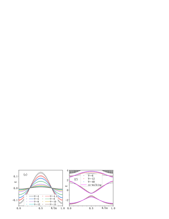
Figure 1: (Color online) The spectra of three fermions (a, b) and bosons (d, e) for $L=61$ and different values of interaction strength. Each point represents an eigenenergy $E$ for a given total momentum $K$, and the red and blue ones correspond to bound states. (c) and (f) show the spectra of 3BSs of fermions and bosons, respectively. The solid lines denote the perturbation results of (2) and (3) which agree well with the ED calculation (symbols). All spectra in either (c) or (f) are shifted by a constant.

Spectra and quantum walks.–

Within the three-particle Hilbert space, we first perform exact diagonalization (ED) of the systems in momentum space. Fig.1 shows spectra of three fermions and bosons, respectively. We observe that the three-particle systems of bosons and fermions host scattering states (SSs), two-body bound states (2BSs) and three-body bound states (3BSs). In the weak interaction region, the spectra only contain one continuum band corresponding to SSs for both three bosons and fermions. However, as the attraction increases the spectrum behave rather statistics-dependently, see Fig.1(a,b,d,e). For the bosonic system, the BSs split from the continuum band when the interaction $V$ becomes stronger. The whole spectra contain three isolated spectra with gaps in between. Three mini-bands of the 3BSs, which are energetically lower than that of the 2BSs (blue part in Fig.1(b,e)), remarkably form competitive QWs in time evolution. The SSs band is continuous with highest energies. In contrast, for the fermionic system there is only one continuum SSs band as long as the interaction $|V|<1$. Bands of the SSs, 2BSs and 3BSs are energetically separated for large attractions. The 3BSs only constitute one mini-band with the lowest energy, and it becomes more and more flat when the attraction increases.

Now we employ time evolving block decimation (TEBD) algorithm Vidal1 ; Iyer:2013 to numerically simulate the three-particle continuous-time QWs. They are governed by the unitary time-evolution $|\psi(t)\rangle=e^{-iHt}|\psi(t=0)\rangle$, in contrast to the discrete-time QWs which obey a successive single-time evolution governed by ‘shift’ and ‘coin’ operators Cedzich1 ; Arnault1 ; Destri1 ; Bisio1 . Here we set the initial state $|\psi(t=0)\rangle=a^{\dagger}_{-1}a^{\dagger}_{0}a^{\dagger}_{1}|0\rangle$ with three particles at the three central neighbouring sites. Open boundary conditions are used under the cumulative truncation errors in the order of $10^{-8}$. We study time evolutions of density distribution $n_{j}(t)=\langle\psi(t)|a^{\dagger}_{j}a_{j}|\psi(t)\rangle$ and density-density correlation function $C_{i,j}(t)=\langle\psi(t)|\hat{n}_{i}\hat{n}_{j}|\psi(t)\rangle$, which preserve the symmetries $n_{j}(t)|_{V}=n_{j}(t)|_{-V}$ and $C_{i,j}(t)|_{V}=C_{i,j}(t)|_{-V}$ Yu1 ; Supplemental . We thus only consider the attractive interaction in our study.

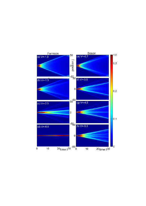
Figure 2: (Color online) Time-evolutions of density distribution for three-fermion (a-d) and boson (e-h) systems with $L=101$ and different values of attractions, see text. Results (a)-(d) match analytic results for the XXZ Heisenberg model Liu1 .

In Fig.2 we show time-evolutions of density distribution for three-particle QWs. Both the weakly interacting bosons and fermionic systems with $|V|<1$ have the same form of evolution, i.e. a single ballistic expansion light-cone is established because of the single continuum band of the SSs. For the fermionic system with the interaction $|V|>1$, an inner cone emerges with a slower and linearly moving wave front, indicating the formation of BSs. Continuing to increase the interaction, the third innermost cone forms. From outer to inner, three cones correspond to ballistic expansions of the SSs, 2BSs and 3BSs, respectively, see Fig.2(c). As $|V|$ is further increased, the cones of SSs and 2BSs gradually fade away and only the light-cone of the 3BSs remains. The speed of wave front (SWF) of the SSs is independent of interaction, i.e., it is always $2$, showing a maximal group velocity (MGV) of non-interacting particles. But SWFs for 2BSs and 3BSs decrease when the interaction $|V|$ increases. Note that the results of Fig. 2 (a)-(d) for fermions match nicely the corresponding analytic results for the equivalent XXZ Heisenberg model Liu1 .

For the bosonic system, besides the outer cone for SSs, an inner cone for the BSs emerges as long as $V$ is nonzero. When the interaction increases, the SWF of this inner cone first decreases and then stops decreasing at a fixed value due to the band structure of the 3BSs. Then the third innermost cone shows up, its SWF first decreases and then increases to a finite value, see Fig.2 (f), (g), (h) and Fig.S9 in Supplemental . This unique behaviour of innermost cone is caused by the interplay of the 2BS and the 3BS. For a large enough attraction, the evolution contains only two cones which are both related to the three mini-bands of 3BSs.

Moreover, the density-density correlation function $C_{i,j}(t)$ also provides an important statistical nature of the three-particle QWs Supplemental . It significantly marks the difference between co-walking and individual walking. The co-walking particles bound together and move as a single composite particle, revealing the togetherness of quasiparticles. The density-density correlations for co-walking show few lines (5 lines) at ($i=j\pm d$) with $d=1,\,2$ in the ($i,j$) plane, a signature of the co-walking. In Fig.3, we show $C_{i,j}(t)$ for both fermionic and bosonic systems at time $t=22$ (they are free from the boundary effects). For a small $|V|$, the correlation function shows (anti-)bunching behaviour with (off-)diagonal correlations at the wave front in the (fermionic) bosonic system. As $|V|$ increases, bunching and anti-bunching correlations fade away, and correlations on four minor diagonal lines ($i=j\pm 1,\,2$) are gradually enhanced with respect to a statistics-dependent pace, see the subsets in Fig.3. In contrast to the co-walking of two bosons Qin1 , the co-walking of three bosons remarkably shows expansive wave fronts due to the existence of the mini-bands of the 3BSs.

Many-body perturbation and Bloch oscillations.– Under a strong attraction, one can treat the hopping as a perturbation to the interaction term in the Hamiltonian (1), see Takahashi1 . After projecting onto the subspace of the 3BSs, an effective single-particle model can be derived explicitly. For the fermionic case, by using the third order perturbation, an effective single-particle Hamiltonian for the co-walking of three fermions is given by Supplemental

$$\hat{H}^{\mathrm{F}}_{\mathrm{eff}}=-\frac{J^{3}}{V^{2}}\sum_{j}(c^{\dagger}_{j}c_{j+1}+\mathrm{H.c.}),$$ (2)

where $c^{\dagger}_{j}=a^{\dagger}_{j-1}a^{\dagger}_{j}a^{\dagger}_{j+1}$. The spectrum of this single-particle Hamiltonian (2) reads $E^{\mathrm{F}}_{\mathrm{eff}}(K)=-\frac{2J^{3}}{V^{2}}\mathrm{cos}(K)$ with a MGV $v^{\mathrm{F}}=2J^{3}/V^{2}$, see footnote2 . In Fig.1(c), we show the spectrum of the 3BSs for the fermionic system, where the dots denote numerical result obtained from ED and lines are obtained from the effective single-particle Hamiltonian (2). Both results agree well as $|V|$ increases. The MGV $v^{\mathrm{F}}$ is also in a good agreement with the SWF of the 3BSs Supplemental . We observe from Eq.(2) that the ballistic expansion of three-fermion co-walking becomes very slow as $|V|$ increases.

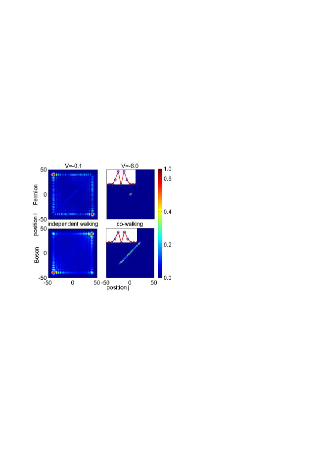
Figure 3: (Color online) Density-density correlation functions $C_{i,j}$ for both fermionic (upper panel) and bosonic (lower panel) systems with a size $L=101$ at the time $t=22$. Corresponding profiles $C_{i=0,j}$ around $j=0$ are shown in subsets.

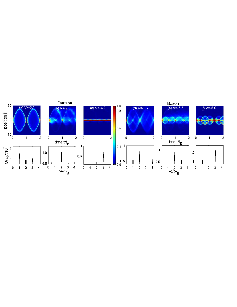
Figure 4: (Color online) Left (a-c) and right (d-f) panels show the time evolutions of density distributions for three and fermions with $L=101$ and $F=0.1$, respectively. Multiple fractional Bloch oscillations are observed. The corresponding frequencies are shown in the bottom row.

The subspace of three-boson co-walking has $3L$-fold degeneracies. The first order perturbation gives an effective single-particle Hamiltonian Supplemental

$$\hat{H}^{\mathrm{B}}_{\mathrm{eff}}=-\sqrt{2}J\sum_{j}(d^{\dagger}_{j}b_{j}+c^{\dagger}_{j}b_{j}+\sqrt{2}d^{\dagger}_{j+1}c_{j}+\mathrm{H.c.})$$ (3)

with three species $b^{\dagger}_{j}=a^{\dagger}_{j-1}a^{\dagger}_{j}a^{\dagger}_{j+1}$, $c^{\dagger}_{j}=\frac{1}{\sqrt{2}}(a^{\dagger}_{j})^{2}a^{\dagger}_{j+1}$, and $d^{\dagger}_{j}=\frac{1}{\sqrt{2}}a^{\dagger}_{j-1}(a^{\dagger}_{j})^{2}$. Obviously, it is independent of $V$. In the momentum space we can get the spectra of the effective Hamiltonian (3), which are shown in Fig. 1 (f) (solid lines), agree well with the ED numerical results (doted lines). The 3BSs have three mini-bands which show two different MGVs, $v^{\mathrm{B}}_{1}\simeq 1$ for the middle mini-band and $v^{\mathrm{B}}_{2}\simeq 0.64$ for other two mini-bands in Fig. 1 (f) (solid lines). $v^{\mathrm{B}}_{1(2)}$ agrees well with the SWF of the outer (inner) cone when $|V|\gg 1$, see Supplemental .

In order to achieve a metrological application of QWs, we add a static force to the Hamiltonian (1)

$$\hat{H}_{\mathrm{Force}}=F\sum_{j}ja^{\dagger}_{j}a_{j}$$ (4)

with $F$ the strength of the applied force and consider the BOs from the same initial state $|\psi(t=0)\rangle=a^{\dagger}_{-1}a^{\dagger}_{0}a^{\dagger}_{1}|0\rangle$.

We illustrate the BOs for fermionic systems in the left panel of Fig.4. For a weak interaction, i.e. $|V|<1$, particles independently undergo a single-particle BO with the amplitude $4J/F$ and the temporal period $t_{B}=2\pi/F$ (frequency $\omega_{B}=F$) Kosevich1 ; Zhang1 . When $|V|>1$, two inner BOs appear successively with smaller amplitudes and shorter periods. From outer to inner there are BOs of the SSs, 2BSs and 3BSs, respectively. Upon further increasing the attraction, the two outer BOs gradually fade away and only the BO of the 3BSs remains, see Supplemental . In order to analyze the periodicity, we introduce a density difference $O(t)=\sum_{j}|n_{j}(t)-n_{j}(t=0)|/L$. From the Fourier transformation $O(\omega)$, we observe the characteristics periodicities of $t_{\mathrm{B}}/2$ and $t_{\mathrm{B}}/3$ (or frequencies $2\omega_{B}$ and $3\omega_{B}$) BOs for 2BSs and 3BSs, respectively, which are called fractional BOs in interacting systems Dias1 ; Khomeriki1 ; Corrielli1 . $O(\omega)$ presents the relative weights of BO modes with different frequencies. In the strong coupling limit, i.e. $|V|\gg 1$, the co-BO of 3BSs of fermions can be described by the effective single-particle Hamiltonian $\hat{H}^{F}_{\mathrm{BO}}=\hat{H}^{\mathrm{F}}_{\mathrm{eff}}+3F\sum_{j}jc^{\dagger}_{j}c_{j}$ with the BO amplitude $4J^{3}/(3V^{2}F)$, which is inversely proportional to $V^{2}$. Here the effective force is $3F$, which leads to the periodicity of co-BO $t_{\mathrm{B}}/3$, as well as the frequency of $3\omega_{\mathrm{B}}$.

Due to the quantum statistical difference, the ground-state degeneracies are different for bosons and fermions, leading to different many-body perturbation processes as well as different dynamics of the BOs, see Fig. 4. The corresponding effective single-particle Hamiltonian, describing the BOs among three mini-bands under an effective force $3F$, is given by

$$\hat{H}^{B}_{\mathrm{BO}}=\hat{H}^{\mathrm{B}}_{\mathrm{eff}}+3F\sum_{j}[jb^{\dagger}_{j}b_{j}+(j+\frac{1}{3})c^{\dagger}_{j}c_{j}+(j-\frac{1}{3})d^{\dagger}_{j}d_{j}],$$ (5)

see Supplemental . We observe that the Landau-Zener tunellings display between two nearby mini-bands Breid1 ; Longhi1 . The amplitude of co-BO $\propto J/3F$ is independent of $V$, showing a larger FI than that of the co-walking of three fermions in next section. Consequently, the periodicity of co-BO of three bosons is $t_{B}/3$ and the frequency is $3\omega_{B}$ that provides an ideal metrological state for a precision measurement of a weak force.

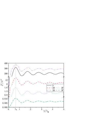
Figure 5: (Color online) The time-dependent quantum FIs $\mathcal{F}/4t^{2}$ vs time $t$ for single- and multi-particle (co)-BOs. Parameters: L=101, V=-10, and $F=0.1$. The FIs are proportional to $t^{3}$ for $t<t_{0}$, while $\mathcal{F}\sim t^{2}$ for $t>t_{0}$.

Fisher information and precision measurement.– The three-boson QWs have a very rich dynamical structure of the co-BOs that leads to an almost interaction-independent co-BO amplitude and high value of FI in the probe of the weak force, see Supplemental . Here the FIs for (co-)BOs presents the precision limit for single parameter $F$. By definition of FI for an unitary process from a pure initial state Braunstein1 ; Braunstein2 ; Liu2 , we can calculate the FIs of single- and multi-particle (co-)BOs Supplemental

$$\mathcal{F} = 4[(\frac{\partial}{\partial F}\langle\psi(t)|)\frac{\partial}{\partial F}|\psi(t)\rangle-|\langle\psi(t)|\frac{\partial}{\partial F}|\psi(t)\rangle|^{2}],$$ (6)

$$= 4t^{2}\Delta H^{Q}(t),$$

where $\Delta H^{Q}(t)$ is the fluctuation of a time-dependent effective Hamiltonian $H^{Q}(t)$ over the initial state $|\psi_{0}\rangle$.

$$\Delta H^{Q}(t) = \langle\psi_{0}|[H^{Q}(t)]^{2}|\psi_{0}\rangle-\langle\psi_{0}|H^{Q}(t)|\psi_{0}\rangle^{2},$$

$$H^{Q}(t) = h[it\cdot\mathrm{ad}_{H_{\mathrm{BO}}}](\partial_{F}H_{\mathrm{BO}}),$$ (7)

with operator function $h[x]=(e^{x}-1)/x$ and adjoint operator $\mathrm{ad}_{G}(C)=[G,C]$. In Fig.5 we show FIs as functions of time for (co)-BOs. Here we denoted single-particle (S), two-boson (2B), two-fermion (2F), three-fermion (3F), and three-boson (3B) (co-)BOs, respectively. We demonstrate that below a characteristic time $t_{0}\approx 0.5t_{B}$, the time scalings of FIs show a surprising power law form $\mathcal{F}\simeq\alpha t^{3}$, where $\alpha$ is a state-dependent constant footnote , also see Supplemental . In contrast to the smallest FI of the three-fermion co-BO with $\alpha\approx 0.024$, the three-boson co-BO has the largest FI with the largest value of $\alpha\approx 1185.485$, then the smallest uncertainty in the measurement of force. The single-particle BO has the second largest FI. For $t>t_{0}$, the FIs for these walk states saturate to the standard quantum limit $\mathcal{F}\simeq 4At^{2}$ with case-dependent constant coefficients $A$.

Conclusions and Discussions.– We have studied continuous-time QWs, BOs and FIs of three bosons and fermions in 1D lattices, which reveal intrinsic and extrinsic roles of quantum statistics, interaction and the gravitational force in the quantum random walks. We have demonstrated that the metrological useful entanglement for high precision measurements of weak forces can be generated under the time evolutions of suitable quantum states. Our method also holds a promise for a quantum-enhanced precision test of the EP through the QWs of three bosons.

The superiority of three-boson co-BO in precision measurement of weak force would provide a potential approach to test the Einstein equivalence principle (EP). Instead of making comparison with the BOs of non-interacting isotopes Tarallo1 , one may test the EP through the BOs of same species of three interacting bosons, see a discussion in Supplemental .

This work is supported by the National Key R&D Program of China No. 2017YFA0304500 and the NKRDP under Grant No. 2016YFA0301503, the NSFC grant No. 11874393, No. 1167420 and No. 12025509. XMC, HTY and HLS equally contribute the numerical and analytical studies for this research. The authors thank Jing Liu and Wei-Dong Li for helpful discussions.

Supplementary material: Multi-particle quantum walks and Fisher information in one-dimensional lattices

I S1. Symmetries in dynamic evolution

For the system with only nearest-neighbour interactions, we can decompose it into odd and even lattices, and define a symmetry operator $W$ which acts on the bipartite lattice via Yu1

$$W^{-1}a_{j}W=(-1)^{j}a_{j}.$$ (S1)

Then we obtain

$$W^{-1}H_{\mathrm{H}}W =-H_{\mathrm{H}},$$

$$W^{-1}H_{\mathrm{F}}W =H_{\mathrm{F}},$$

$$W^{-1}H_{0}W =H_{0},$$ (S2)

with the hopping $H_{\mathrm{H}}=-J\sum_{j}(a^{\dagger}_{j}a_{j+1}+\mathrm{H.c})$, the force $H_{\mathrm{F}}=F\sum_{j}ja^{\dagger}_{j}a_{j}$, and the nearest-neighbour interaction $H_{0}=V\sum_{j}\hat{n}_{j}\hat{n}_{j+1}$. Let the Hamiltonian and initial state be invariant under the time-reversal operator $R$, which only changes the imaginary part, $R^{-1}iR=-i$. With the help of these operators $W$ and $R$, we have

$$n_{j}(t) |_{(V,F)}$$ (S3)

$$=\langle\psi(t)|a^{\dagger}_{j}a_{j}|\psi(t)\rangle$$

$$=\langle\psi(0)|e^{i(H_{H}+H_{0}+H_{\mathrm{F}})t}a^{\dagger}_{j}a_{j}e^{-i(H_{H}+H_{0}+H_{\mathrm{F}})t}|\psi(0)\rangle$$

$$=\langle\psi(0)|(WR)^{-1}e^{i(H_{H}+H_{0}+H_{\mathrm{F}})t}RWa^{\dagger}_{j}a_{j}(WR)^{-1}$$

$$\quad\times e^{-i(H_{H}+H_{0}+H_{\mathrm{F}})t}RW|\psi(0)\rangle$$

$$=\langle\psi(0)|e^{i(H_{H}-H_{0}-H_{\mathrm{F}})t}a^{\dagger}_{j}a_{j}e^{-i(H_{H}-H_{0}-H_{\mathrm{F}})t}|\psi(0)\rangle$$

$$=n_{j}(t)|_{(-V,-F)}.$$

When $F=0$, it reduces to $n_{j}(t)|_{V}=n_{j}(t)|_{-V}$.

Similarly, defining the lattice-reversal operator

$$Q^{-1}a_{j}Q=a_{-j},$$ (S4)

we have

$$Q^{-1}H_{\mathrm{H}}Q =H_{\mathrm{H}},$$

$$Q^{-1}H_{\mathrm{F}}Q =-H_{\mathrm{F}},$$

$$Q^{-1}H_{0}Q =H_{0}.$$ (S5)

And the initial state is invariant under the operator $Q$. Then following Eq.(S3), we obtain

$$n_{j}(t) |_{(V,F)}$$ (S6)

$$=\langle\psi(0)|e^{i(H_{H}-H_{0}-H_{\mathrm{F}})t}a^{\dagger}_{j}a_{j}e^{-i(H_{H}-H_{0}-H_{\mathrm{F}})t}|\psi(0)\rangle$$

$$=\langle\psi(0)|Q^{-1}e^{i(H_{H}-H_{0}-H_{\mathrm{F}})t}QQ^{-1}a^{\dagger}_{j}a_{j}Q$$

$$\quad\times Q^{-1}e^{-i(H_{H}-H_{0}-H_{\mathrm{F}})t}Q|\psi(0)\rangle$$

$$=\langle\psi(0)|e^{i(H_{H}-H_{0}+H_{\mathrm{F}})t}a^{\dagger}_{-j}a_{-j}$$

$$\quad\times e^{-i(H_{H}-H_{0}+H_{\mathrm{F}})t}|\psi(0)\rangle$$

$$=n_{-j}(t)|_{(-V,F)}.$$

Because of these symmetries, we only need to study the dynamics for systems with attractive interactions.

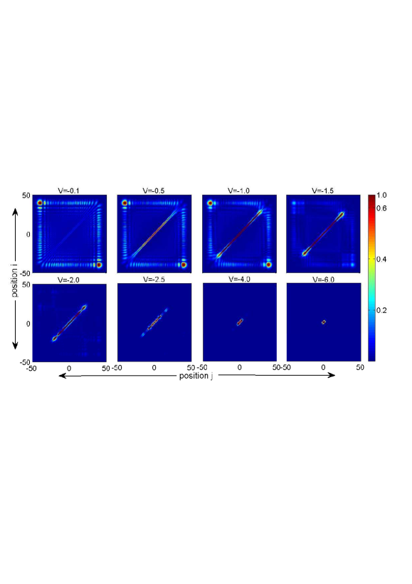
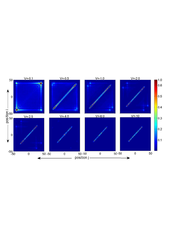
Figure S1: (Color online) Density-density correlation functions $C_{i,j}=\langle\psi(t)|\hat{n}_{i}\hat{n}_{j}|\psi(t)\rangle$ for three-fermion (upper panel) and three-boson (lower panel) QWs, at the time $t=22$ when particles in scattering states are about to collide with boundaries.

II S2. Correlations in three-particle quantum walks

The time-dependent density-density correlation function in real space is defined by

$$C_{i,j}(t)=\langle\psi(t)|\hat{n}_{i}\hat{n}_{j}|\psi(t)\rangle,$$ (S7)

which can be used to study the three-particle quantum walks (QWs). It is very important to distinguish co-walking from independent walking. In a co-walking, particles bound together and move as a single composite particle. Significant correlations show few specific lines ($i=j\pm d$) in the ($i,j$) plane, which give a signature of the co-walking of particles, where $d$ can be integers which depend on the form of interaction and the particle number. For three-particle systems with nearest-neighbour attractions, $d=1,2$.

In Fig.S1 we show density-density correlation functions at the time $t=22$ for both fermionic and bosonic systems. A hard-core bosonic system has the same density-density correlation function as the one for the corresponding fermionic system. The correlation function also has the symmetry $C_{i,j}|_{V}=C_{i,j}|_{-V}$, which can be proved by using the same symmetries as being used above. Therefore, we demonstrate correlations between particles in the attractive systems in Fig.S1. At the time $t=22$, particles in scattering states (fastest) are about to reach the boundaries so that here the boundary effects are negligible.

Like the Hanbury-Brown-Twiss (HBT) interference, for a small attraction $|V|$, the density-density correlation function shows anti-bunching behavior with a major off-diagonal correlation at the wave front for the fermionic system, while it shows bunching behavior with a major diagonal correlation for the bosonic system. A similar behaviour was found in the two-particle QWs Qin1 . When $|V|$ increases, bunching and anti-bunching gradually fade out, and minor diagonal correlation lines ($i=j\pm 1,2$) are enhanced in statistics-dependent QWs. The correlations on these diagonal lines are the robust signature of the three-particle quantum co-walking, showing the existence of three-particle bound states. Whereas, in two-particle QWs, the co-walking is characterized by the correlations on the minor diagonal lines ($i=j\pm 1$) Qin1 . For a system with a very large $|V|$ only the co-walking remains. However, the three-particle co-walking is different from the two-particle case and essentially depends on the statistics of the particles. Detailed discussions about the co-walking are presented in the main text and next section.

III S3. Many-body perturbation and effective single-particle models

Under a strong attraction, three-body bound states of bosons and fermions dominate significantly different QWs and Bloch oscillations (BOs). Three particles behave like a single composite particle and perform quantum co-walking or co-BO. In these cases, we can treat the hopping $H_{\mathrm{H}}$ and additional force $H_{\mathrm{F}}$ as perturbations to the interaction $H_{0}$. To implement the perturbation, we first give the projection operator onto the subspace involved in the three-particle co-walking (co-BO). Then projecting the total Hamiltonian onto the subspace we can obtain effective single-particle models for QWs and BOs of three bosons and fermions.

Following the procedure shown in Ref. Takahashi1 , we first rewrite the Hamiltonian as

$$H = H_{0}+H_{1},$$

$$H_{1} = H_{\mathrm{H}}+H_{\mathrm{F}},$$ (S8)

and treat $H_{1}$ as a perturbation to $H_{0}$. We assume that $H_{0}$ has a discrete degenerate level $E_{0}$, the subspace spanned by corresponding degenerate states is denoted by $U_{0}$, and the projection operator onto $U_{0}$ is denoted by $P_{0}$. We designate the subspace of perturbed eigenstates as $U$ and its corresponding projection operator as $P$. Here $P$ is given by the following integral of resolvent

$$P =\frac{1}{2\pi i}\oint_{C}dz(z-H_{0}-H_{1})^{-1}$$ (S9)

$$=\frac{1}{2\pi i}\oint_{C}dz(z-H_{0})^{-1}\sum_{n=0}^{\infty}[H_{1}(z-H_{0})^{-1}]^{n}.$$

Contour $C$ contains no eigenvalues of $H_{0}$ except $E_{0}$ in the complex plane. Using $(z-H_{0})^{-1}=(z-E_{0})^{-1}P_{0}+(1-P_{0})(z-H_{0})^{-1}$, we obtain

$$P=P_{0}-\sum_{n=1}^{\infty}\sum_{k_{1}+k_{2}+...+k_{n+1}=n,k_{i}\geq 0}S^{k_{1}}H_{1}S^{k_{2}}H_{1}...H_{1}S^{k_{n+1}},$$ (S10)

with

$$S^{0} = -P_{0},$$

$$S^{k} = [(1-P_{0})/(E_{0}-H_{0})]^{k}\quad\mathrm{for}\quad k\geq 1.$$ (S11)

Considering a transformation from a state $|\phi\rangle$ in $U_{0}$ to a state $|\psi\rangle$ in $U$:

$$|\psi\rangle=\Gamma|\phi\rangle,\quad\Gamma\equiv PP_{0}(P_{0}PP_{0})^{-1/2},$$ (S12)

$$(P_{0}PP_{0})^{-1/2}\equiv P_{0}+\sum_{n=1}^{\infty}\frac{(2n-1)!!}{(2n)!!}[P_{0}(P_{0}-P)P_{0}]^{n}.$$

We can obtain

$$\Gamma^{\dagger}\Gamma=P_{0},$$

$$\langle\Gamma\phi|\Gamma\phi^{\prime}\rangle=\langle\phi|\phi^{\prime}\rangle,$$ (S13)

for any $|\phi\rangle,|\phi^{\prime}\rangle\in U_{0}$. Then the eigenvalue problem $H|\psi\rangle=E|\psi\rangle$ is replaced by

$$h|\phi\rangle=E|\phi\rangle,\quad h\equiv\Gamma^{\dagger}H\Gamma.$$ (S14)

$h$ is the effective Hamiltonian in $U_{0}$ subspace. Next we will use this perturbation theory to treat QWs and BOs in the three-particle systems.

III.1 A. Fermions

The unperturbed Hamiltonian $H_{0}$ has three eigenvalues for the three-fermion system:
(i) $E_{0}=2V$ for the $L$-fold degenerate ground states $\{|G_{j}\rangle=|j-1,j,j+1\rangle\}$, which are three-body bound states,
(ii) $E_{j_{1}j_{2}}=V$ for two-body bound states $\{|E_{j_{1}j_{2}}\rangle=|j_{1},j_{1}+1,j_{2}\rangle:j_{2}\neq j_{1}-1,...,j_{1}+2\}$,
(iii)$E_{j_{1}j_{2}j_{3}}=0$ for scattering states $\{|E_{j_{1}j_{2}j_{3}}\rangle=|j_{1},j_{2},j_{3}\rangle:j_{1}+1<j_{2}<j_{3}-1\}$.
$|j_{i}\rangle$ denotes a fermion located at the site $j_{i}$, and $L$ is the total number of lattice sites. The three-fermion co-walking (co-BO) only involves the subspace spanned by $L$ independent ground states $|G_{j}\rangle$. The projection operator onto the subspace is

$$P_{0}=\sum_{j}|G_{j}\rangle\langle G_{j}|,$$ (S15)

and corresponding orthogonal projection operator reads

$$S= \sum_{j_{1},j_{2}}\frac{1}{E_{0}-E_{j_{1}j_{2}}}|E_{j_{1}j_{2}}\rangle\langle E_{j_{1}j_{2}}|$$ (S16)

$$+\sum_{j_{1},j_{2},j_{3}}\frac{1}{E_{0}-E_{j_{1}j_{2}j_{3}}}|E_{j_{1}j_{2}j_{3}}\rangle\langle E_{j_{1}j_{2}j_{3}}|.$$

Expanding Eq.(S10) and Eq.(S12), up to third order perturbations, the effective Hamiltonian reads

$$H_{\mathrm{eff}}^{(3)} = E_{0}P_{0}+P_{0}H_{1}P_{0}+P_{0}H_{1}SH_{1}P_{0}$$

$$+P_{0}H_{1}SH_{1}SH_{1}P_{0}$$

$$-\frac{1}{2}(P_{0}H_{1}P_{0}H_{1}S^{2}H_{1}P_{0}+P_{0}H_{1}S^{2}H_{1}P_{0}H_{1}P_{0}).$$

Substituting $P_{0}$ (S15), $S$ (S16) and $H_{1}$ into the above equation, we obtain the non trivial effective Hamiltonian

$$H_{\mathrm{eff}}^{(3)} = h_{1}^{(3)}+h_{2}^{(3)},$$

$$h_{1}^{(3)} = -\frac{J^{3}}{V^{2}}\sum_{j}(|G_{j}\rangle\langle G_{j+1}|+|G_{j+1}\rangle\langle G_{j}|),$$

$$h_{2}^{(3)} = 3F\sum_{j}j|G_{j}\rangle\langle G_{j}|.$$ (S18)

$h_{1}^{(3)}$ and $h_{2}^{(3)}$ correspond to the hopping and force terms, respectively. In order to capture the single-particle nature, we introduce creation operators $c^{\dagger}_{j}$ for states $|G_{j}\rangle$ ($c^{\dagger}_{j}|0\rangle=a^{\dagger}_{j-1}a^{\dagger}_{j}a^{\dagger}_{j+1}|0\rangle$). Then the three-fermion co-walking (co-BO) obeys the following effective single-particle Hamiltonian

$$\hat{H}^{\mathrm{F}}_{\mathrm{eff}}=-\frac{J^{3}}{V^{2}}\sum_{j}(c^{\dagger}_{j}c_{j+1}+\mathrm{H.c.})+3F\sum_{j}jc^{\dagger}_{j}c_{j}.$$ (S19)

For fermions, the first and second orders are trivial, because the translation of a three-fermion bound state can not be realized by hopping of one or two fermions. The third order is nontrivial and is the only process for the three-body bound state moving right. In Fig.S2 (a) we show long-time evolution of density distribution for a fermionic system with $F=0$ and a very large attraction. The straight line has a slope $v^{\mathrm{F}}=2J^{3}/V^{2}$ which shows a maximal group velocity of the effective single-particle Hamiltonian at the absence of the external force ($F=0$). This analytical straight line indicates the wave front of three-fermion co-walking and is consistent with the numerical calculation. We observe that such consistence holds quite well as long as $V/J\geq 3$, although the perturbation theory requires only for $J\ll V$.

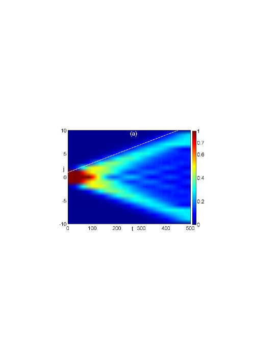
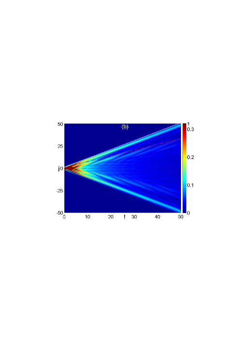
Figure S2: (Color online) (a) Long-time evolution of density distribution for the fermionic system with $L=21$, $F=0$ and $V=-10$. The straight line corresponds to the position of wave front, with a slope equaling the maximal group velocity $v^{F}=2/V^{2}$. (b) Time evolution of density distribution for the bosonic system with $L=101$, $F=0$ and $V=-40$. Straight lines have slopes $v^{B}_{1,2}\simeq 1,0.64$.

III.2 B. Bosons

For the three-boson system, the unperturbed Hamiltonian $H_{0}$ also has three eigenvalues:
(i) $E_{0}=2V$ for the $3L$-fold degenerate ground states (three-body bound states) $\{|G^{(1)}_{j}\rangle=|j-1,j,j+1\rangle\}\cup\{|G^{(2)}_{j}\rangle=|j^{2},j+1\rangle\}\cup\{|G^{(3)}_{j}\rangle=|j-1,j^{2}\rangle\}$,
(ii) $E_{1}=V$ for two-body bound states $\{|E_{j_{1}j_{2}}\rangle=|j_{1},j_{1}+1,j_{2}\rangle:j_{2}\neq j_{1}-1,...,j_{1}+2\}$,
(iii)$E_{2}=0$ for scattering states $\{|D_{j_{1}j_{2}j_{3}}\rangle=|j_{1},j_{2},j_{3}\rangle:j_{1}+1<j_{2}<j_{3}-1\}\cup\{|D_{j_{1}j_{2}}\rangle=|j^{2}_{1},j_{2}\rangle:j_{2}\neq j_{1}\pm 1\}\cup\{|D_{j_{1}}\rangle=|j^{3}_{1}\rangle\}$. Here $|j^{n}_{1}\rangle$ means that there are $n$ bosons at lattice site $j_{1}$. The three-boson co-walking (co-BO) involves the subspace spanned by $3L$-fold degenerate ground states $|G^{(i=1,2,3)}_{j}\rangle$. States with different $i$ or $j$ are orthogonal to each other. The projection operator onto the subspace

$$P_{0}=\sum_{j}(|G^{(1)}_{j}\rangle\langle G^{(1)}_{j}|+|G^{(2)}_{j}\rangle\langle G^{(2)}_{j}|+|G^{(3)}_{j}\rangle\langle G^{(3)}_{j}|).$$ (S20)

Unlike the fermionic system, the bosonic one can have more than one particle per site. States with different $i$ in the subspace can be transformed into each other by the perturbation Hamiltonian $H_{1}$. Then the first order effective Hamiltonian is non trivial, while the zeroth order is proportional to the identity operator. This is quite different from the three-fermion and two-particle cases Qin1 . After a lengthy calculation the first order effective Hamiltonian reads

$$H^{(1)}_{\mathrm{eff}}= P_{0}H_{1}P_{0}=h^{(1)}_{1}+h^{(1)}_{2},$$

$$h^{(1)}_{1}= -\sqrt{2}J\sum_{j}(|G^{(3)}_{j}\rangle\langle G^{(1)}_{j}|+|G^{(2)}_{j}\rangle\langle G^{(1)}_{j}|$$

$$+\sqrt{2}|G^{(3)}_{j+1}\rangle\langle G^{(2)}_{j}|+\mathrm{H.c.})$$

$$h^{(1)}_{2}= F\sum_{j}3j|G^{(1)}_{j}\rangle\langle G^{(1)}_{j}|+F\sum_{j}(3j+1)|G^{(2)}_{j}\rangle\langle G^{(2)}_{j}|$$ (S21)

$$+F\sum_{j}(3j-1)|G^{(3)}_{j}\rangle\langle G^{(3)}_{j}|.$$

Then we introduce effective single-particle creation operators. Explicitly, $b^{\dagger}_{j}|0\rangle=a^{\dagger}_{j-1}a^{\dagger}_{j}a^{\dagger}_{j+1}|0\rangle$, $c^{\dagger}_{j}|0\rangle=\frac{1}{\sqrt{2}}(a^{\dagger}_{j})^{2}a^{\dagger}_{j+1}|0\rangle$, and $d^{\dagger}_{j}|0\rangle=\frac{1}{\sqrt{2}}a^{\dagger}_{j-1}(a^{\dagger}_{j})^{2}|0\rangle$. The effective single-particle Hamiltonian for three-boson co-walking (co-BO) is given by

$$H^{\mathrm{B}}_{\mathrm{eff}}= -\sqrt{2}J\sum_{j}(d^{\dagger}_{j}b_{j}+c^{\dagger}_{j}b_{j}+\sqrt{2}d^{\dagger}_{j+1}c_{j}+\mathrm{H.c.})$$ (S22)

$$+F\sum_{j}3jb^{\dagger}_{j}b_{j}+F\sum_{j}(3j+1)c^{\dagger}_{j}c_{j}$$

$$+F\sum_{j}(3j-1)d^{\dagger}_{j}d_{j}.$$

It is independent of $V$. The amplitudes are proportional to $J$, while amplitudes of nontrivial higher orders are much smaller than the leading order term when $J/V\ll 1$. On the other hand, the first order perturbation of the force term is also nontrivial. The force can not transfer states in the three-body bound state subspace. It thus is diagonal and only causes energy shifts of different states.

After transforming it into the momentum space, the hopping part of the effective single-particle Hamiltonian reads

$$H^{\mathrm{B}}_{\mathrm{eff}}=-J\sum_{k}\Psi^{\dagger}_{k}\left(\begin{matrix}0&\sqrt{2}&\sqrt{2}&\\ \sqrt{2}&0&2e^{-ik}&\\ \sqrt{2}&2e^{ik}&0&\end{matrix}\right)\Psi_{k}.$$ (S23)

with $(\Psi_{k})^{\mathrm{T}}=(b_{k},c_{k},d_{k})$. We see that analytical eigenvalues are quite complicated. Therefore we just presented numerical results in the main text.

The Hamiltonian Eq.(S23) consists with the three mini-band spectra. The maximal group velocity for the middle mini-band is about $v^{\mathrm{B}}_{1}\simeq 1$, and the other two mini-bands have the same maximal group velocity $v^{\mathrm{B}}_{2}\simeq 0.64$. In Fig.S2 (b) we show the time evolution of density distribution for a three-boson system with $F=0$ and a very large attraction. The white straight and red dot lines show slopes of $v^{\mathrm{B}}_{1}$ and $v^{\mathrm{B}}_{2}$, respectively. They truly indicate the movements of the wave fronts for two inner light cones when $V/J\geq 6$, revealing an important signature of the three-boson co-walking.

IV S4. Two-body bound states in three-particle quantum walks

In this section, we demonstrate that two-body physics can emerge in three-particle QWs and BOs. The quantum walks of two particles is quite contrast to the situation in the quantum walks of three particles. The co-BO states are also quite different in the two-body bound state sector. To this end, we employ the initial state $|\psi_{1}(t=0)\rangle=a^{\dagger}_{-1}a^{\dagger}_{0}a^{\dagger}_{2}|0\rangle$, with one particle being away from the other neighbouring two. The initial state is an eigenstate in 2BS subspace of the interaction term $H_{0}$. Similar symmetries in dynamics still hold, and we only study systems with attractive interactions.

IV.1 A. Quantum walks

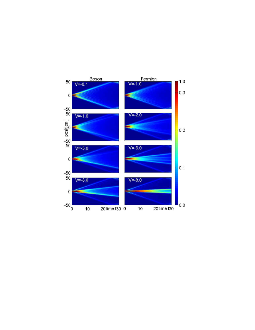
Figure S3: (Color online) Time evolutions of density distribution for three-boson (left collum) and fermion (right collum) QWs, from the initial state $|\psi_{1}\rangle=a^{\dagger}_{-1}a^{\dagger}_{0}a^{\dagger}_{2}|0\rangle$. The inner-cones show the QWs of the two-body bound states.

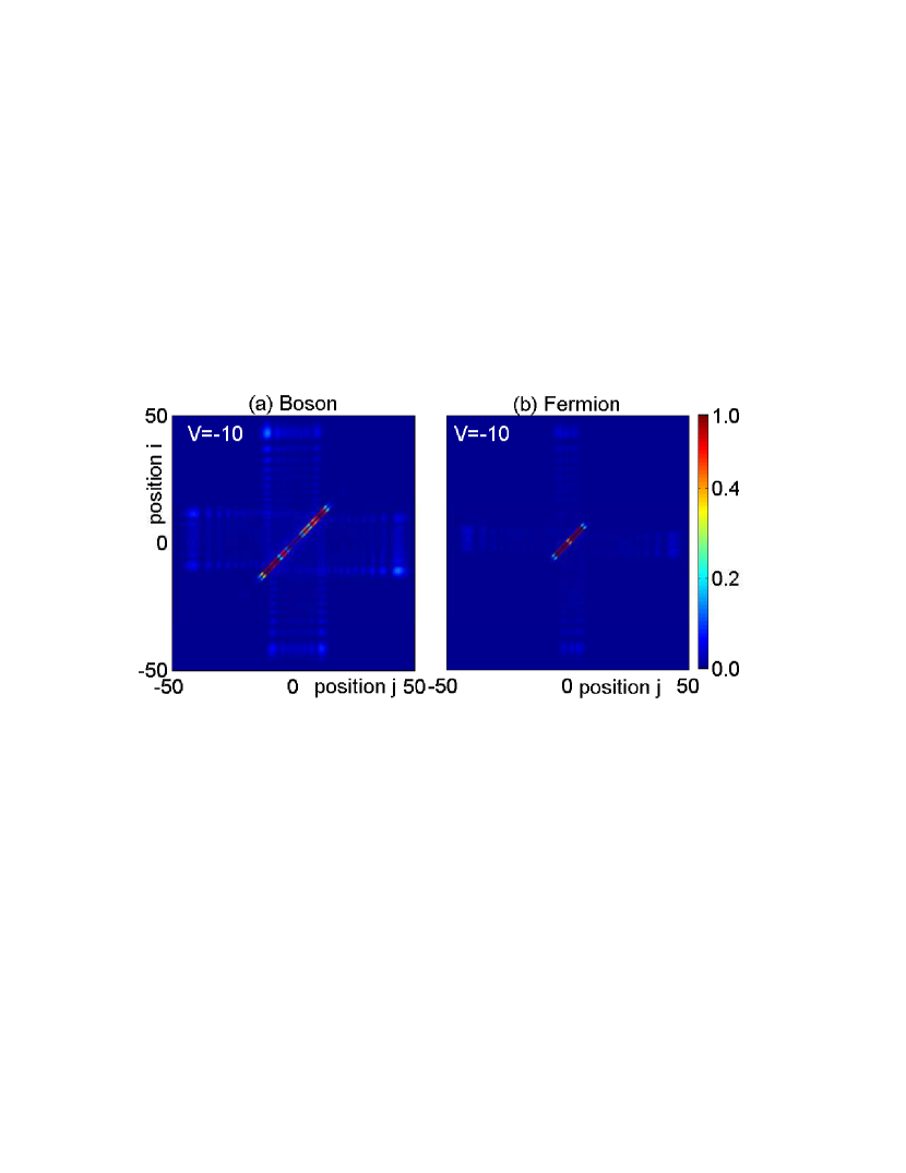
Figure S4: (Color online) Density-density correlation functions $C_{i,j}$ at the time $t=22$, for three-boson (a) and fermion (b) QWs from the initial state $|\psi_{1}\rangle=a^{\dagger}_{-1}a^{\dagger}_{0}a^{\dagger}_{2}|0\rangle$. For a strong interaction, i.e., $V=-10$, the correlation functions mainly contain two diagonal lines at $i=j\pm 1$ in the ($i,j$) plane, showing the presence of two-particle bound states. The big “Cross” in the correlation for bosons clearly shows the interference between the pair and single particle.

In Fig.S3 we show time evolutions of density distribution for three-particle QWs from the initial state $|\psi_{1}\rangle$. In the non-interacting limit, both bosonic and fermionic systems show single-particle nature and experience a ballistic expansion with speed of wave front (SWF) $2$. For a bosonic system with non-zero attraction, there is an inner light-cone and corresponding SWF decreases as the attraction increases. While for the fermionic system, the inner light-cone exists only when $|V|>1$, and corresponding SWF has a different decay pace from the bosonic one. Compared with QWs from the initial state $|\psi\rangle=a^{\dagger}_{-1}a^{\dagger}_{0}a^{\dagger}_{1}|0\rangle$ shown in the main paper (see also in Fig.S8 and Fig.S9 in last section), here the outer light-cone does not fade out as $|V|$ increases, and a third innermost light-cone shows up for systems with intermediate attractions but disappears at large attractions. The expansion contains two light-cones for systems with very large attractions, and the SWF of inner light-cone for bosons is larger than that for fermions.

The density-density correlation function for QWs from the initial state $|\psi_{1}\rangle$ shows similar behaviours as for the initial state $|\psi\rangle$, when the attraction is not very large. (Anti)bunching behavior for bosonic (fermionic) systems with weak attractions fades out as the attraction increases, along with the gradually enhanced diagonal correlations. In Fig.S4 we show correlation functions for systems with a large attraction. Both bosonic and fermionic systems have similar behaviours. Correlation functions mainly contain two diagonal lines at $i=j\pm 1$ in the ($i,j$) plane, which indicates the presence of two-particle bound states. It also presents a characteristic of two-particle quantum co-walking, see Qin1 . We observe the two-particle pair in inner light-cone and the ’free’ particle in outer light-cone in time evolutions. While the interference between the single particle and the pair is visible in Fig.S4. The big “Cross” in the correlation for bosons clearly shows the interference between the pair and single particle. But such an interference is much weaker in the QWs of the three fermions. In the following, we will derive an effective Hamiltonian from which we can conceive such subtle dynamics of two-body bound states in the QWs of three particles.

Under a strong attraction, an effective single-particle model also can be derived for QWs from the initial state $|\psi_{1}\rangle$. After projecting onto the subspace of 2BSs, the second order perturbation gives

$$H^{F(B)}_{\mathrm{eff}}=H_{p}^{F(B)}+H_{s}+H_{t}$$ (S24)

with

$$H_{p}^{F(B)}= \frac{(3)J^{2}}{V}\sum_{j_{1},j_{2}}(a^{\dagger}_{j_{1}-1,j_{2}}a_{j_{1}j_{2}}+\mathrm{h.c.}),$$ (S25)

$$H_{s}= -J\sum_{j_{1},j_{2}}(a^{\dagger}_{j_{1},j_{2}+1}a_{j_{1}j_{2}}+\mathrm{h.c.}),$$ (S26)

$$H_{t}=- J\sum_{j}(a^{\dagger}_{j-2,j+1}a_{j,j-2}+a^{\dagger}_{j+2,j}a_{j,j+3})$$

$$- \frac{J^{2}}{V}\sum_{j}(a^{\dagger}_{j+2,j-1}a_{j,j+3}+a^{\dagger}_{j-2,j+2}a_{j,j-2})$$

$$+ \frac{J^{2}}{V}\sum_{j}(a^{\dagger}_{j-3,j+1}a_{j,j-3}+a^{\dagger}_{j+1,j-1}a_{j,j+3})$$

$$+ \frac{J^{2}}{V}\sum_{j}(a^{\dagger}_{j-2,j+1}a_{j,j-3}+a^{\dagger}_{j+2,j-1}a_{j,j+3})$$

$$+ \frac{J^{2}}{V}\sum_{j}(a^{\dagger}_{j+2,j}a_{j,j+4}+a^{\dagger}_{j-2,j+2}a_{j,j-2})$$

$$+ \frac{J^{2}}{V}\sum_{j}(a^{\dagger}_{j+3,j}a_{j,j+4}+a^{\dagger}_{j-1,j+2}a_{j,j-2}).$$ (S27)

In the above equations, we defined effective single-particle operators $a^{\dagger}_{j_{1},j_{2}}|0\rangle=|E_{j_{1},j_{2}}\rangle$ for 2BSs, where $j_{1}$ and $j_{2}$ denote positions of the two-particle pair and the ’free’ particle away from the pair, respectively. The summation on $j_{2}$ is restricted in the set $\{j_{2}\neq j_{1}-2,..,j_{1}+2\}$. “F(B)” stands for the fermionic (bosonic) system. The first term $H_{p}^{F(B)}$ indicates the hoping occurs in the paired particle and the second term $H_{s}$ shows the hopping occurs in the single particle. While the last term $H_{t}$ shows the interchange process between the pair and single particle. Moreover, the effective Hamiltonians $H_{p}^{F(B)}$ govern the dynamics of two-particle pair, which are the same as the Hamiltonians for two-particle quantum co-walkings Qin1 , where the spectra of $H_{p}^{F(B)}$ read $E_{p}^{F(B)}(K)=\frac{(3)2J^{2}}{V}\mathrm{cos}(K)$. The maximal group velocities $\upsilon_{p}^{F(B)}=(3)2J^{2}/V$, which determine the SWFs of the inner light-cone. The bosonic pair expanses three times faster than the fermionic one. Unlike for the three-particle quantum co-walkings, maximal group velocities for both systems decrease quickly as $|V|$ increases. Hamiltonian $H_{s}$ governs the dynamics of the ’free’ particle in 2BSs, which is the same as the single-particle Hamiltonian with a maximal group velocity $2J$. Finally, the effective Hamiltonian $H_{t}$ describes interference between the two-particle pair and the ’free’ particle, see the Fig.S4.

IV.2 B. Bloch oscillations

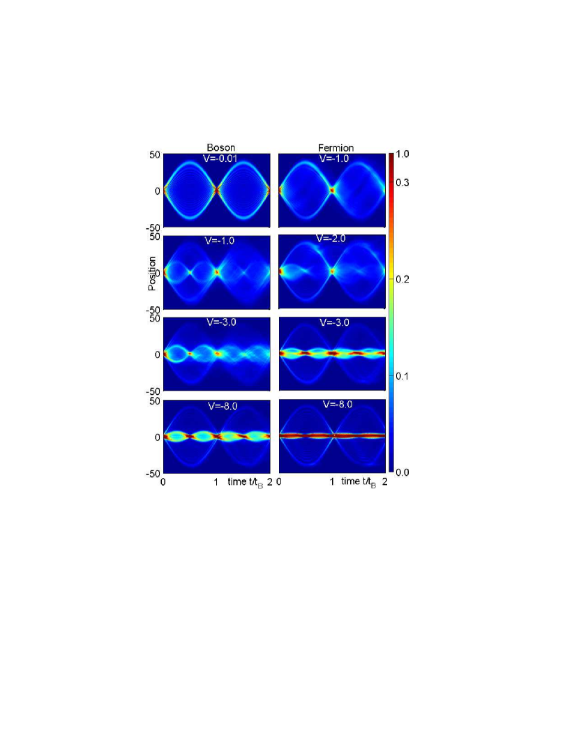
Figure S5: (Color online) Time evolutions of density distribution for three-boson (left column) and fermion (right column) BOs from the initial state $|\psi_{1}\rangle$. $L=101$ and $F=0.1$. Inner cycles show the two-body bound state BOs in the QWs of three particles.

In this subsection, we study BOs from the initial state $|\psi_{1}\rangle$. The Hamiltonian of an additional force is the same ($H_{\mathrm{F}}=F\sum_{j}ja^{\dagger}_{j}a_{j}$) for both bosonic and fermionic systems. In Fig.S5 we show BOs for both bosonic and fermionic systems with different attractions. For fermionic systems with $|V|<1$ and non-interacting bosons, the particles show the single-particle BO independently, with an oscillation amplitude $4J/F$ and a period $t_{B}=2\pi/F$. As the attraction increases, the single-particle BO does not fade out. A gradually enhanced inner BO appears with a temporal period $t_{B}/2$. Its amplitude decreases as the attraction increases and has different decay paces for bosons and fermions. For a large attraction, the amplitude of inner BO for bosons is much larger than that for fermions.

Under large attractions, effective single-particle models for BOs from the initial state $|\psi_{1}\rangle$ are

$$H_{\mathrm{BO}}^{F(B)}=H^{F(B)}_{\mathrm{eff}}+H_{1F}+H_{2F},$$ (S28)

with

$$H_{1F} = F\sum_{j_{1},j_{2}}j_{2}a^{\dagger}_{j_{1},j_{2}}a_{j_{1},j_{2}},$$

$$H_{2F} = F\sum_{j_{1},j_{2}}(2j_{1}+1)a^{\dagger}_{j_{1},j_{2}}a_{j_{1},j_{2}}.$$ (S29)

They are derived by up to second order perturbations. $H^{F(B)}_{\mathrm{eff}}$ were presented in Eq.(S24). $H_{s}+H_{F}$ governs the BO of ’free’ particle in 2BSs, which are the same as the Hamiltonian for single-particle BO. $H_{p}^{F(B)}+H_{2F}$ describes the effective single-particle behavior of the two-particle pair in 2BSs. The two-particle pair undergoes a co-BO with the amplitude $(3)4J^{2}/(VF)$ and the period $t_{B}/2$. Except the three times relation in amplitudes of the co-BOs, bosons and fermions have the same behavior and no Landau-Zener tunnelling exists.

V S5. Quantum Fisher information

According to Ref.Liu1 , quantum Fisher information for an unitary process $U=e^{-itH}$ from a pure initial state $|\psi_{0}\rangle$ is given by

$$\mathcal{F}=4\left\{\left[\frac{\partial}{\partial F}\langle\psi(t)|\right]\frac{\partial}{\partial F}|\psi(t)\rangle-|\langle\psi(t)|\frac{\partial}{\partial F}|\psi(t)\rangle|^{2}\right\},$$ (S30)

where $|\psi(t)\rangle=e^{-itH}|\psi_{0}\rangle$. The force $F$ in Hamiltonian $H$ is to be the measured parameter in the precision measurement of the gravitational force. The limit on the precision of measuring the parameter $F$ is described by the quantum Cramér-Rao bound Liu1

$$\Delta F\geq\frac{1}{\sqrt{\mathcal{F}}}.$$ (S31)

The larger quantum Fisher information indicates a higher measurement precision. Therefore, we can use quantum Fisher information to quantify the performance of different processes in the precision measurement of gravity.

We consider the effective single-particle Hamiltonian

$$H=J^{\prime}\sum_{j}[c^{\dagger}_{j}c_{j+1}+\mathrm{h.c.}]+F^{\prime}\sum_{j}c^{\dagger}_{j}c_{j},$$ (S32)

with

$$J^{\prime} = -J,F^{\prime}=F,\mathrm{for\thinspace single-particle\thinspace BO};$$ (S33)

$$J^{\prime} = 3J^{2}/V,F^{\prime}=2F,\mathrm{for\thinspace two-boson\thinspace co-BO};$$

$$J^{\prime} = J^{2}/V,F^{\prime}=2F,\mathrm{for\thinspace two-fermion\thinspace co-BO};$$

$$J^{\prime} = -J^{3}/V^{2},F^{\prime}=3F,\mathrm{for\thinspace three-fermion\thinspace co-BO},$$

and the one for three-boson co-BO

$$H= -\sqrt{2}J\sum_{j}[d^{\dagger}_{j}c_{j}+b^{\dagger}_{j}c_{j}+\sqrt{2}d^{\dagger}_{j+1}b_{j}+h.c.]$$

$$+3F\sum_{j}[jc^{\dagger}_{j}c_{j}+(j+\frac{1}{3})b^{\dagger}_{j}b_{j}+(j-\frac{1}{3})d^{\dagger}_{j}d_{j}].$$

Pure initial states for (co-)BOs are in the same form $|\psi_{0}\rangle=c^{\dagger}_{0}|0\rangle$.

In order to calculate Eq.(S30), we first introduce some useful formulaes. Given $\rho=e^{G}$ which is a function of $F$, we have

$$\frac{\partial\rho}{\partial F}=\int^{1}_{0}e^{sG}(\partial_{F}G)e^{(1-s)G}ds,$$

$$e^{G}Ae^{-G}=e^{\mathrm{ad}_{G}}(A),$$ (S35)

where $\mathrm{ad}_{G}$ is the adjoint superoperator, i.e., $\mathrm{ad}_{G}(A)=[G,A]$. Then we have

$$(\partial_{F}\rho)\rho^{-1} = h[\mathrm{ad}_{G}](\partial_{F}G),$$ (S36)

$$\rho^{-1}(\partial_{F}\rho) = g[\mathrm{ad}_{G}](\partial_{F}G)$$ (S37)

with operator functions $h[x]=(e^{x}-1)/x$ and $g[x]=(1-e^{-x})/x$. Given above introduced formulaes, the expression of quantum Fisher information reduces to

$$\mathcal{F}=4t^{2}\{\langle\psi_{0}|[H^{Q}(t)]^{2}|\psi_{0}\rangle-\langle\psi_{0}|H^{Q}(t)|\psi_{0}\rangle^{2}\},$$ (S38)

where we have introduced a time-dependent effective Hamiltonian

$$H^{Q}(t)=h[it\cdot\mathrm{ad}_{H}](\partial_{F}H).$$ (S39)

In numerical calculations, we treat the Hamiltonian as a vector in the space spanned by the basis $\mathfrak{C}=\{|j,j^{\prime}\rangle\equiv c^{\dagger}_{j}c_{j^{\prime}},j,j^{\prime}=-M,...,M\}$. Then the adjoint superoperator acts as an operator in the space $\mathfrak{C}$. Diagonalizing the adjoint operator, we can numerically get the effective Hamiltonian and quantum Fisher informations which are shown in Fig. 5 in the main paper. $\mathcal{F}/4t^{2}$ (or the fluctuation of time-dependent effective Hamiltonian $\Delta H^{Q}$) increases monotonously and is approximately linear dependence of the time $t$ for the time $t<t_{0}$. Whereas it approaches to a constant with damping oscillations for $t>t_{0}$. Regarding to the lowest order approximation, it can be approximated by the piece-wise function, which shows a linear dependence of the time $t$ when $t<t_{0}$ and approaches to a constant when $t>t_{0}$. Thus we have the Fisher information $\mathcal{F}=\alpha t^{3}$ when $t<t_{0}$, while $\mathcal{F}=At^{2}$ when $t>t_{0}$. The coefficients $\alpha$ are extracted by numerical fitting.

The BOs of ideal Bose gas can be harnessed for the precision measurement of gravity Ferrari1 ; Tarallo1 . For our model in the weakly interacting region, SSs dominate the BO with the frequency $\omega_{B}=F/h$ and particles experience force $F$ which is proportional to the gravitational force. For the strongly interacting region 3BSs dominate the BO with the frequency $\omega_{B}=3F/h$ and the three-particle formed composite quasiparticle experiences an effective force $3F$. Such exact three times relation between themeasurement of gravity frequencies of the BOs of single and three bosons enables a high precision testing EP. Here the precision is free from the mass ratio uncertainty of the two isotopes in addition to the precision limit $1/t^{3/2}$, beyond the fundamental limit $1/t$.

VI S6. Additional figures

In this subsection, we show additional figures in order to further understand the spectra, QWs and BOs of three interacting particles. In Fig.S6 and Fig.S7, we show spectra of three fermions (Fig. S6) and bosons (Fig.S7) at different interaction strengths. The figures are obtained from the numerical exact diagonalization in three-particle Hilbert space. Periodic boundary conditions and the conservation of total momentum $K$ are used in the calculations. For three bosons, the Hilbert space is spanned by the basis

$$\mathfrak{B}=\{|k_{1}k_{2}k_{3}\rangle=N_{k_{1}k_{2}k_{3}}a^{\dagger}_{k_{1}}a^{\dagger}_{k_{2}}a^{\dagger}_{k_{3}}|0\rangle\},$$

with $0\leq k_{1}\leq k_{2}\leq k_{3}<L$. Here $N_{k_{1}k_{2}k_{3}}$ is the normalization factor and $a^{\dagger}_{k}$ is the creation operator of a particle with momentum $k\frac{2\pi}{L}$. For three fermions, the Hilbert space is spanned by the basis

$$\mathfrak{F}=\{|k_{1}k_{2}k_{3}\rangle=a^{\dagger}_{k_{1}}a^{\dagger}_{k_{2}}a^{\dagger}_{k_{3}}|0\rangle\},$$

with $0\leq k_{1}<k_{2}<k_{3}<L$. Each base vector has a total momentum $K=\mathrm{mod}(\sum_{l=1}^{3}k_{l},L)*\frac{2\pi}{L}$. We classify the three-particle Hilbert space into a series of subspaces, each with a given total momentum $K$. After transforming the Hamiltonian into the momentum space, it is very easy to numerically generate the matrix representation in each subspace. Then we can diagonalize the Hamiltonian for a pretty large size $L$. Fig.S6 and Fig.S7 show important statistics-and-interaction-dependent nature in many-particle spectra.

In Fig.S8 and Fig.S9, we show time evolutions of density distribution for three-fermion (Fig.S8) and three-boson (Fig.S9) systems with $L=101$, $F=0$ at different interaction strengths, where the initial state is set up $|\psi(t=0)\rangle=a^{\dagger}_{-1}a^{\dagger}_{0}a^{\dagger}_{1}|0\rangle$. Time evolving block decimation (TEBD) algorithm is used. The maximal bond dimension of matrix product state $\chi=120$. Fifth-order Suzuki-Trotter expansion under open boundary condition is used for the unitary time evolution, and the time step $\delta t=10^{-3}$. Total cumulative truncation errors are controlled on or less than the order of $10^{-8}$. For systems with same parameters but different $L$, the numerical results show finite-size and boundary effects. Such effects are negligible before particles collide with boundaries.

In Fig.S10 and Fig.S11, we show time evolutions of density distribution and corresponding $O(t)$ and $O(\omega)$ for three-fermion (Fig.S10) and three-boson (Fig.S11) systems with $L=101$, $F=0.1$ and different attractions. The maximal bond dimension of matrix product state $\chi=150$. The time step for unitary time evolution is set up with $\delta t=10^{-3}t_{B}$, where $t_{B}=2\pi/F$ is the period of single-particle BO. Total cumulative truncation errors are controlled on or less than the order of $10^{-7}$. The statistics-dependent BOs are demonstrated in the dynamics of three-particle systems.

Figure S6: Three-fermion spectra for systems with $L=61$, $F=0$ and different interaction strengths of $V$.

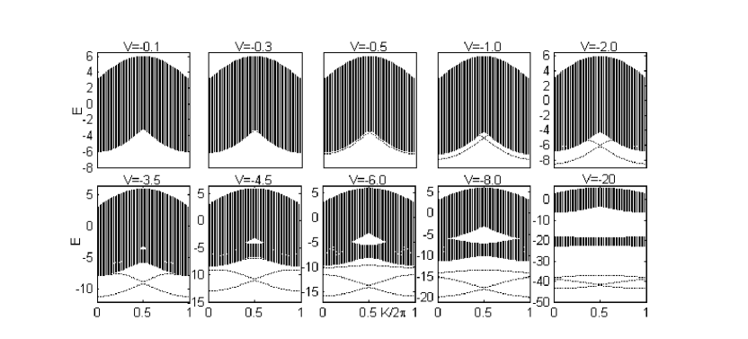
Figure S7: Three-boson spectra for systems with $L=61$, $F=0$ and different interaction strengths.

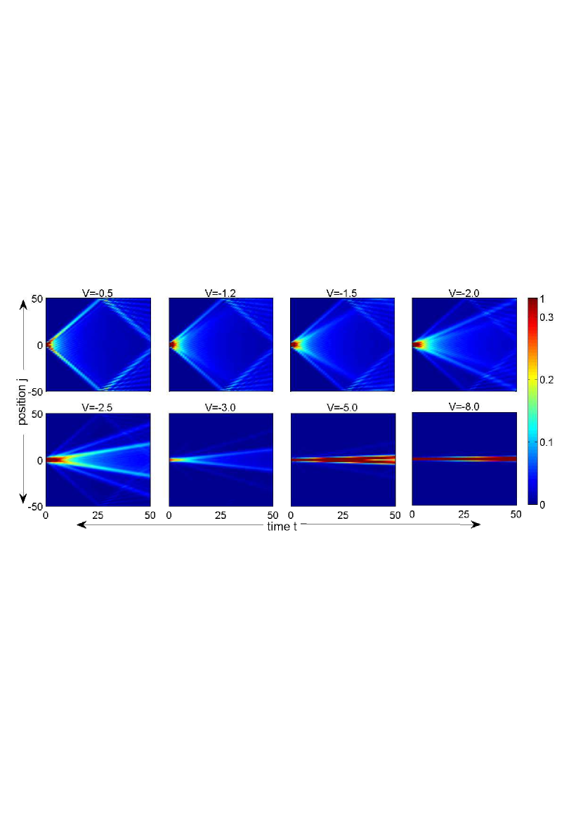
Figure S8: (Color online) Time evolutions of density distribution for three-fermion systems with $L=101$, $F=0$ and different attraction strengths.

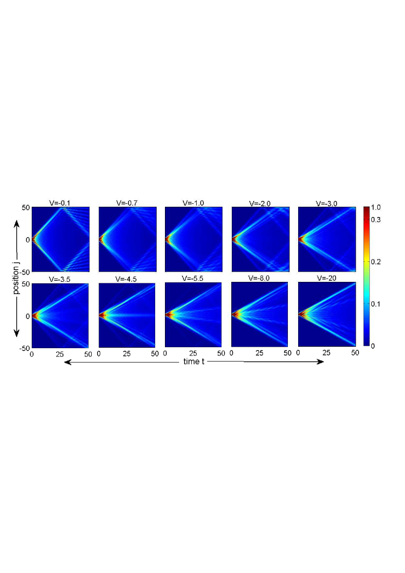
Figure S9: (Color online) Time evolutions of density distribution for three-boson systems with $L=101$, $F=0$ and different attraction strengths.

Figure S10: (Color online) Time evolutions of density distribution (left column), and corresponding $O(t)$ (middle column) and $O(\omega)$ (right column) for three-fermion systems with $L=101$, $F=0.1$ and different attraction strengths.

Figure S11: (Color online) Time evolutions of density distribution (left column), and corresponding $O(t)$ (middle column) and $O(\omega)$ (right column) for three-boson systems with $L=101$, $F=0.1$ and different attraction strengths.

References

- (1) Y. Aharonov, L. Davidovich, and N. Zagury, Phys. Rev. A 48, 1687 (1993).
- (2) J. Kempe, Contemporary Phys. 44, 307 (2003).
- (3) A. Ambainis, Int. J. Quantum. Inform. 1, 507 (2003).
- (4) A. M. Childs, D. Gosset, and Z. Webb, Science 339, 791 (2013).
- (5) F. Zatelli, C. Benedetti, and M. G. A. Paris, arXiv:2010.12448.
- (6) S. E. Venegas-Andraca, Quant. Info. Proc. 11, 1015 (2012).
- (7) J. K. Asbóth, Phys. Rev. B 86, 195414 (2012).
- (8) S. Lloyd, J. Phys. Conf. Ser. 302, 012037 (2011).
- (9) J. Wang and K. Manouchehri, Physical Implementation of Quantum Walks (Springer, Berlin, Heidelberg, 2013).
- (10) T. Kitagawa, M. A. Broome, A. Fedrizzi, M. S. Rudner, E. Berg, I. Kassal, A. Aspuru-Guzik, E. Demler, and A. G. White, Nat. Commun. 3, 882 (2012).
- (11) Y. E. Kraus, Y. Lahini, Z. Ringel, M. Verbin, and O. Zilberberg, Phys. Rev. Lett. 109, 106402 (2012); M. Verbin, O. Zilberberg, Y. E. Kraus, Y. Lahini, and Y. Silberberg, Phys. Rev. Lett. 110, 076403 (2013).
- (12) V. V. Ramasesh, E. Flurin, M. Rudner, I. Siddiqi, and N. Y. Yao, Phys. Rev. Lett. 118, 130501 (2017).
- (13) C. Destri, and H. J. De Vega, Nucl. Phys. B 290, 363 (1987).
- (14) C. Cedzich, T. Rybár, A. H. Werner, A. Alberti, M. Genske, and R. F. Werner, Phys. Rev. Lett. 111, 160601 (2013).
- (15) A. Bisio, G. M. D’Ariano, P. Perinotti, and A. Tosini, Phys. Rev. A 97, 032132 (2018).
- (16) P. Arnault, B. Pepper, and A. Pérez, Phys. Rev. A 101, 062324 (2020).
- (17) A. Ahlbrecht, A. Alberti, D. Meschede, V. B. Scholz, A. H. Werner, and R. F. Werner, New J. Phys. 14, 073050 (2012).
- (18) T. Fukuhara, P. Schauß, M. Endres, S. Hild, M. Cheneau, I. Bloch, and C. Gross, (London) 502, 76 (2013).
- (19) M. Karski, L. Förster, J.-M. Choi, A. Steffen, W. Alt, D. Meschede, and A. Widera, Science 325, 174 (2009).
- (20) H. Schmitz, R. Matjeschk, C. Schneider, J. Glueckert, M. Enderlein, T. Huber, and T. Schaetz, Phys. Rev. Lett. 103, 090504 (2009); F. Zähringer, G. Kirchmair, R. Gerritsma, E. Solano, R. Blatt, and C. F. Roos, Phys. Rev. Lett. 104, 100503 (2010).
- (21) A. Schreiber, K. N. Cassemiro, V. Potoček, A. Gábris, P. J. Mosley, E. Andersson, I. Jex, and C. Silberhorn, Phys. Rev. Lett. 104, 050502 (2010); M. A. Broome, A. Fedrizzi, B. P. Lanyon, I. Kassal, A. Aspuru-Guzik, and A. G. White, Phys. Rev. Lett. 104, 153602 (2010); A. Schreiber, K. N. Cassemiro, V. Potoček, A. Gábris, I. Jex, and C. Silberhorn, Phys. Rev. Lett. 106, 180403 (2011).
- (22) T. Fukuhara, A. Kantian, M. Endres, M. Cheneau, P. Schauß, S. Hild, D. Bellem, U. Schollwöck, T. Giamarchi, C. Gross, I. Bloch, and S. Kuhr, Nat. Phys. 9, 235 (2013).
- (23) J. Du, H. Li, X. Xu, M. Shi, J. Wu, X. Zhou, and R. Han, Phys. Rev. A 67, 042316 (2003).
- (24) A. Peruzzo , M. Lobino, J. C. F. Matthews, N. Matsuda, A. Politi, K. Poulios, X. Zhou, Y. Lahini, Nur Ismail, K. Wörhoff, Y. Bromberg, Y. Silberberg, M. G. Thompson, J. L. OBrien, Science 329, 1500 (2010).
- (25) K. Mayer, M. C. Tichy, F. Mintert, T. Konrad, and A. Buchleitner Phys. Rev. A 83, 062307 (2011).x
- (26) R. H. Brown and R. Q. Twiss, Nature (London) 177, 27 (1956).
- (27) M. Hillery, Science 329, 1477 (2010).
- (28) L. Sansoni, F. Sciarrino, G. Vallone, P. Mataloni, A. Crespi, R. Ramponi, and R. Osellame, Phys. Rev. Lett. 108, 010502 (2012).
- (29) A. S. Solntsev, A. A. Sukhorukov, D. N. Neshev, and Y. S. Kivshar, Phys. Rev. Lett. 108, 023601 (2012).
- (30) Y. Lahini, M. Verbin, S. D. Huber, Y. Bromberg, R. Pugatch, and Y. Silberberg, Phys. Rev. A 86, 011603(R) (2012).
- (31) Y. Omar, N. Paunkovič, L. Sheridan, and S. Bose, Phys. Rev. A 74, 042304 (2006).
- (32) C. Benedetti, F. Buscemi, and P. Bordone, Phys. Rev. A 85, 042314 (2012).
- (33) X. Qin, Y. Ke, X. Guan, Z. Li, N. Andrei, and C. Lee, Phys. Rev. A 90, 062301 (2014).
- (34) P. M. Preiss, R. Ma, M. E. Tai, A. Lukin, M. Rispoli, P. Zupancic, Y. Lahini, R. Islam, and M. Greiner, Science 347, 1229 (2015).
- (35) L. Wang, L. Wang, and Y. Zhang, Phys. Rev. A 90, 063618 (2014).
- (36) L. L. H. Lau, and S. Dutta, Quantum walk of two anyons across a statistical boundary, arXiv:2012.03977.
- (37) M. Ganahl, E. Rabel, F. H. Essler, and H. G. Evertz, Phys. Rev. Lett. 108, 077206 (2012).
- (38) P. L. Krapivsky, J. M. Luck, and K. Mallick, J. Phys. A 48, 475301 (2015).
- (39) D. Wiater, T. Sowiński, and J. Zakrzewski, Phys. Rev. A 96,043629 (2017).
- (40) D. Iyer, H. Guan, and N. Andrei, Phys. Rev. A 87, 053628 (2013).
- (41) I. Siloi, C. Benedetti, E. Piccinini, J. Piilo, S. Maniscalco, M. G. A. Paris, and P. Bordone, Phys. Rev. A 95, 022106 (2017).
- (42) A. Beggi, I. Siloi, C. Benedetti, E. Piccinini, L. Razzoli, P. Bordone and M. G. A. Paris, Eur. J. Phys. 39, 065401 (2018)
- (43) S. Sarkar and T. Sowiński, Phys. Rev. A 102, 043326 (2020).
- (44) W. Liu and N. Andrei, Phys. Rev. Lett. 112, 257204 (2014).
- (45) Z. A. Geiger, K. M. Fujiwara, K. Singh, R. Senaratne, S. V. Rajagopal, M. Lipatov, T. Shimasaki, R. Driben, V. V. Konotop, T. Meier and D. M. Weld, Phys. Rev. Lett. 120, 213201 (2018).
- (46) G. Ferrari, N. Poli, F. Sorrentino, and G. M. Tino, Phys. Rev. Lett. 97, 060402 (2006).
- (47) M. G. Tarallo, T. Mazzoni, N. Poli, D. V. Sutyrin, X. Zhang, and G. M. Tino, Phys. Rev. Lett. 113, 023005 (2014).
- (48) W. Liu, Y. Ke, L. Zhang, and C. Lee, Phys. Rev. A 99, 063614 (2019).
- (49) M. Atala, M. Aidelsburger, J. T. Barreiro, D. Abanin, T. Kitagawa, E. Demler and I. Bloch, Nat. Phys. 9, 795(2013).
- (50) I. Carusotto, L. Pitaevskii, S. Stringari, G. Modugno, and M. Inguscio, Phys. Rev. Lett. 95, 093202(2005).
- (51) C. W. Helstrom, Quantum Detection and Estimation Theory, Academic Press, New York, 1976.
- (52) L. Pezzè, A. Smerzi, M. K. Oberthaler, R. Schmied, and P. Treutlein, Rev. Mod. Phys. 90, 035005 (2018).
- (53) J. Liu, H. Yuan, X. M. Lu and X. Wang, J. Phys. A, 53, 023001 (2020).
- (54) H. Sun, B. Yang, H. Y. Wang, Z. Y. Zhou, G. X. Su, H. N. Dai, Z. S. Yuan, J. W. Pan, arXiv: 2009.01426.
- (55) B. Yang, H. Sun, R. Ott, H. Y. Wang, T. V. Zache, J. C. Halimeh, Z. S. Yuan, P. Hauke, J. W. Pan, arXiv:2003.08945.
- (56) P. Jordan and E.Wigner, Z. Phys. 47, 631 (1928).
- (57) C. N. Yang, and C. P. Yang, Phys. Rev. 150, 321 (1966); 150, 327 (1966); 151, 258 (1966).
- (58) M. Takahashi, Thermodynamics of One-Dimensional Solvable Models (Cambridge University Press, Cambridge, 1999).
- (59) C. Lee, Phys. Rev. Lett. 93, 120406 (2004).
- (60) G. Vidal, Phys. Rev. Lett. 91, 147902 (2003); Phys. Rev. Lett. 93, 040502 (2004).
- (61) J. Yu, N. Sun, and H. Zhai, Phys. Rev. Lett. 119, 225302 (2017).
- (62) In the Supplemental Material, we give more details for the symmetries in dynamic evolution, correlation functions in three-particle QWs, the derivation of effective single-particle models for co-walkings and co-BOs, the two-body physics in three-particle QWs, the calculation of Fisher information and additional figures for spectra, QWs and BOs.
- (63) M. Takahashi, J. Phys. C, 10, 1289 (1977).
- (64) Y. A. Kosevich, and V. V. Gann, J. Phys. Condens. Matter 25, 246002(2013).
- (65) H. Zhang, Y. Zhai, and X. Chen, J. Phys. B 47, 025301(2014).
- (66) W. S. Dias, E. M. Nascimento, M. L. Lyra, and F. A. B. F. de Moura, Phys. Rev. B 76, 155124 (2007).
- (67) R. Khomeriki, O. Krimer, M. Haque, and S. Flach, Phys. Rev. A 81, 065601 (2010).
- (68) G. Corrielli, A. Crespi, G. Della Valle, S. Longhi, and R. Osellame. Nat. Commun. 4, 1555 (2013).
- (69) B. M. Breid, D. Witthaut, and H. J. Korsch, New J. Phys. 8, 110 (2006).
- (70) S. Longhi, Phys. Rev. B 86, 075144 (2012).
- (71) S. L. Braunstein and C. M. Caves, Phys. Rev. Lett. 72, 3439 (1994).
- (72) S. L. Braunstein, C. M. Caves and G. J. Milburn, Ann. Phys. 247, 135 (1996).
- (73) The numerical values for the states 3B, S, 2B, 2F, 3F, respectively. The errors of such power-law simulation are less than 3%.
- (74) The third-order amplitude is proportional to . The fourth and higher orders are also nontrivial but their amplitudes are much smaller than the third order when .

References

- (1) J. Yu, N. Sun, and H. Zhai, Phys. Rev. Lett. 119, 225302 (2017).
- (2) X. Qin, Y. Ke, X. Guan, Z. Li, N. Andrei, and C. Lee, Phys. Rev. A 90, 062301 (2014).
- (3) M. Takahashi, J. Phys. C, 10, 1289 (1977).
- (4) J. Liu, H. Yuan, X. M. Lu and X. Wang, J. Phys. A, 53, 023001 (2020).
- (5) G. Ferrari, N. Poli, F. Sorrentino, and G. M. Tino, Phys. Rev. Lett. 97, 060402 (2006).
- (6) M. G. Tarallo, T. Mazzoni, N. Poli, D. V. Sutyrin, X. Zhang, and G. M. Tino, Phys. Rev. Lett. 113, 023005 (2014).