Multipole vortex patch equilibria for active scalar equations
Abstract.
We study how a general steady configuration of finitely-many point vortices, with Newtonian interaction or generalized surface quasi-geostrophic interactions, can be desingularized into a steady configuration of vortex patches. The configurations can be uniformly rotating, uniformly translating, or completely stationary. Using a technique first introduced by Hmidi and Mateu [36] for vortex pairs, we reformulate the problem for the patch boundaries so that it no longer appears singular in the point-vortex limit. Provided the point vortex equilibrium is non-degenerate in a natural sense, solutions can then be constructed directly using the implicit function theorem, yielding asymptotics for the shape of the patch boundaries. As an application, we construct new families of asymmetric translating and rotating pairs, as well as stationary tripoles. We also show how the techniques can be adapted for highly symmetric configurations such as regular polygons, body-centered polygons and nested regular polygons by integrating the appropriate symmetries into the formulation of the problem.
1. Introduction
1.1. Historical discussion
In this note we consider the generalized surface quasi-geostrophic (gSQG) equations, which describe the evolution of the potential temperature through the transport equation
| (1.1) |
Here while is a real parameter. The vector field is the flow velocity and the fractional Laplacian operator is of convolution type, defined by
with
| (1.2) |
where is the gamma function. This model was proposed by Córdoba et al. [12] as an interpolation between Euler equations and the surface quasi-geostrophic model, which correspond to and , respectively.
The main purpose of this note is to show the existence of new families of periodic global solutions of (1.1) in the vortex patch setting, namely when is the characteristic function of finite collection of bounded domains. Such patterns are a special class of Yudovich solutions where is merely bounded and integrable. Yudovich solutions are known to be unique and to exist globally in time in the case of Euler equations [54], but for the situation is more delicate because the velocity field is in general not Lipschitz. Nonetheless, when the initial datum has a patch structure, one can locally construct a unique solution which remains a patch. The motion of the boundary of the patch is governed by so-called contour dynamics equations; see [20, 47]. It is worth mentioning that, while the boundary’s regularity is globally preserved for [11, 3], for numerical evidence [12] suggests singularity formation in finite time.
There are very few explicit solutions to the gSQG and Euler equations. The only known explicit simply-connected vortex patch solutions are the Rankine vortex, which is stationary, and the Kirchhoff ellipses [29] for the Euler equation, which are rotating. Nevertheless, a family of uniformly rotating patches with -fold symmetry, called V-states, was numerically computed by Deem and Zabusky [17]. Later, Burbea [4] gave an analytical proof of their existence, based on a conformal mapping parametrization and local bifurcation theory. Recently, Burbea’s branches of solutions were extended to global ones [32]. The regularity and the convexity of the V-states have been investigated in [37, 32, 8]. Similar research has been carried out for the gSQG equations: The construction of simply connected V-states was established in [30, 7], and their boundary regularity was discussed in [8].
We point out that there is a large literature dealing with rotating vortex patches and related problems. For instance, we mention the existence results of rotating patches close to Kirchhoff’s ellipses [34, 8], multiply-connected patches [38, 16, 35, 14, 46, 26], patches in bounded domains [15], non-trivial rotating smooth solutions [9] and rotating vortices with non-uniform densities [24]. The radial symmetry properties of stationary and uniformly-rotating solutions was studied in a series of works [19, 33, 28].
All of the above analytical results treat connected patches. The first numerical works revealing the existence of translating symmetric pairs of simply connected patches for Euler equation are due to Deem and Zabusky [17] and Pierrehumbert [45]. Similar studies were performed by Saffman and Szeto in [50] for the symmetric co-rotating vortex pairs and by Dritschel [18] for asymmetric pairs. Later, Turkington gave in [51] an analytical proof using variational arguments, where he considered an unbounded fluid domain with symmetrically arranged vortex patches rotating about the origin. Implementing the same approach, Keady [39] proved the existence of translating pairs of symmetric patches and Wan [52] studied the existence and stability of desingularizations of a general system of rotating point vortices. Very recently, Godard-Cadillac, Gravejat and Smets [25] extended Turkington’s result to the gSQG equations, while Ao, Dávila, Del Pino, Musso and Wei [1] have obtained related families of smooth solutions via gluing techniques. See [41, 42, 44, 49, 53] for additional references on multiply connected patches.
The variational arguments [51, 39, 25] do not give much information about the shape of the vortex patches, or about the uniqueness of solutions. In [36], however, Hmidi and Mateu gave a direct proof showing the existence of co-rotating and counter-rotating vortex pairs, using an elegant desingularization of the contour dynamics equations and an application of the implicit function theorem. The same technique was implemented for the desingularization of the asymmetric pairs [31], Kármán street [21] and the vortex polygon [22]. See [6] for related results where point vortices are instead desingularized into doubly-connected patches. We mention that, using more sophisticated Nash–Moser techniques, Gómez-Serrano, Park and Shi [27] have very recently constructed stationary configurations of multi-layered patches with finite kinetic energy. Also, García and Haziot [23] have combined ideas from [36] and [32] to prove a global bifurcation result for co-rotating and counter-rotating pairs.
In this note we show how the technique in [36] can be extended to arbitrary configurations of finitely-many point vortices. For a general configuration, the problem reduces via Lyapunov–Schmidt to a finite-dimensional nonlinear equation. Under an natural non-degeneracy assumption on the point vortex configuration alone, one can instead simply apply a modified version of the implicit function theorem. For highly symmetric configurations, we may also simplify the problem by reformulating it in spaces which take these symmetries into account.
1.2. Statement of the general result
Recall that the gSQG point vortex model for interacting vortices in the complex plane is given by the Hamiltonian system
| (1.3) |
where are the point vortex locations, are the circulations and
| (1.4) |
The case corresponds to the classical point vortex Eulerian interaction. A general review about the -vortex problem and vortex statics can be found in [2] for the Newtonian interaction and [48] for gSQG interactions. We are concerned with periodic solutions for which the configuration of vortices is instantaneously moving as a rigid body, so that
| (1.5) |
where here is the constant linear velocity and is the constant angular velocity. Such solutions are known as relative equilibria or vortex crystals. Explicitly solving (1.5), we see that whenever we can shift coordinates so that . Thus there is no loss of generality in restricting our attention to equilibria which are either rotating with and , translating with and , or stationary with .
Setting , (1.3) reduces to the algebraic system
| (1.6) |
where here . Taking real and imaginary parts, this defines a mapping with values in .
Definition 1.1.
Informally stated, our first result is the following; see Theorems 2.7 and 2.8 for a precise version.
Theorem 1.2.
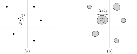
Let . Then any non-degenerate solution of (1.6) can be desingularized into a family of vortex patch equilibria depending smoothly on a small parameter measuring the size of the patches.
See Figure 1 for an illustration.
Remark 1.3.
As we shall see later in Theorems 2.7 and 2.8, the vortex patches in Theorem 1.2 are small perturbations of the unit disk, whose boundaries are given by conformal parametrizations which can be explicitly expanded to any order in the small parameter . In particular, the conformal parametrizations of the boundaries have the explicit Fourier asymptotic expansions
Furthermore, with slight modifications in the proof we can show that the boundary of each vortex patches belongs to for any fixed . The range of would be not uniform with respect to but would shrink to zero as goes to infinity. However, using the approach developed in [8], we expect that the conformal mappings possess holomorphic extensions outside of a small disc and thus that the boundaries are analytic. In the Euler case, the analyticity of sufficiently smooth patch boundaries could alternatively be proved using the same technique as in [32].
Remark 1.4.
The leading-order ratios between the sizes of the patches can be specified a priori. Moreover, the range of is uniform as some of these ratios are sent to zero, allowing us to recover solutions involving a combination of point vortices and vortex patches. See Remark 2.9 for more details.
1.3. Applications
There are many point vortex equilibria satisfying the non-degeneracy assumption in Theorem 1.2. We shall give several examples where this assumption can be easily checked and the resulting vortex patch solutions are, to the best of our knowledge, new.
The most elementary solutions to (1.6) are co-rotating and counter-rotating vortex pairs. A family of asymmetric co-rotating pairs is given by
| (1.9) |
where , and ; see Figure 2(a). In the time-dependent problem, the two vortices steadily rotate about the origin with angular velocity . Counter-rotating pairs given by
| (1.10) |
instead steadily translate along the -axis; see Figure 2(b). We also consider asymmetric stationary tripoles of the form
| (1.11) | ||||
where ; see Figure 2(c). Note that all of these above configurations are invariant under reflections about the -axis. Furthermore, horizontal translations of (1.10) and rotations of (1.9) are also solutions.

As we shall see in Section 3, these configurations are non-degenerate in the sense of Definition 1.1. Using Theorem 1.2, they can therefore be desingularized into steady vortex patch equilibria. As no two vortices in (1.9) or (1.11) can be identified with one another, the same is true of the corresponding vortex patches. While the two vortices in (1.10) can be identified, this symmetry is broken if we require the leading-order ratio between the sizes of the patches to be different from . For the pairs, this extends the desingularization result of [31], obtained in the Eulerian case , to gSQG equations (1.1) with . To the best of our knowledge, the asymmetric tripole patch solutions are new both for the Euler and gSQG equations. Furthermore, this appears to be the first existence proof for stationary solutions to the gSQG equations involving multiple patches; see [27] for stationary solutions to the Euler equations with multiple multi-layered patches and [26] for stationary doubly connected solutions to the gSQG equations.
Theorem 1.6.
Let and , and let be as above. Then, the following results hold true.
-
(i)
For any sufficiently small, there are two strictly convex domains , -fold symmetric, perturbations of the unit disc, and real numbers , such that
generates a co-rotating vortex pair for (1.1) with angular velocity .
-
(ii)
For any sufficiently small, there are two strictly convex domains , -fold symmetric, perturbations of the unit disc, and real numbers , such that
generates a counter-rotating vortex pair for (1.1) with speed .
-
(iii)
For any sufficiently small, there are three strictly convex domains , -fold symmetric, perturbations of the unit disc, and two real numbers , such that
generates a stationary vortex tripole for (1.1).
Remark 1.7.
By sending some of to zero, we can recover configurations involving a mixture of vortex patches and point vortices; see Remark 2.9.
Remark 1.8.
The reflection symmetry property can be checked using the boundary equations, the uniqueness of the constructed curve of solutions and invariance under reflections about the -axis of the point vortex configuration; see Section 3.
While the above examples are asymmetric and have only two or three vortices, there are other well-known point vortex equilibria which are highly symmetric and have many vortices. When seeking similarly symmetric desingularizations of such equilibria, it convenient to integrate these additional symmetries into the statement of the problem. In particular, the relevant non-degeneracy conditions on the point vortex equilibria can be much simpler to verify than Definition 1.1.
As a concrete example, we consider two concentric regular -gons with a vortex at each vertex, and assume that the vortices of a same polygon have the same vorticity or . We place, in addition, a point vortex at the center of the regular -gons with intensity . More specifically, we are concerned with the system of point vortices
| (1.12) |
The value corresponds to the configuration where the vertices of the polygons are radially aligned with each other and refers to the case where the vertices are out-of-phase by an angle . If we assume that (1.12) performs a perpetual uniform rotation, then we may easily check that the system of equations in (1.6) can be reduced to a system of two real equations:
| (1.13) |
Observe that the last system is linear in and , and, thus, under a simple non-degeneracy condition we can explicitly solve the system (1.13) for and .
For the sake of clarity we shall give an elementary statement about the desingularization of these configurations; for a complete statement see Theorem 4.3.
Theorem 1.9.
Let , , , , and let be a solution of (1.13) satisfying the non-degeneracy conditions (4.7) and (4.9). Then, for any sufficiently small, there are three strictly convex domains , perturbations of the unit disc, and a real number such that
| (1.14) |
generates a rotating solution for (1.1) with some constant angular velocity . Moreover is -fold symmetric and , are -fold symmetric.
See Figure 3 for an illustration.
Remark 1.10.
Remark 1.11.
Remark 1.12.
The proof can be easily adapted to the rotating vortex polygon (with in (1.14)) and which has been studied in [1, 25, 51, 22]. This remains equally true for the body-centered polygonal configurations (), treated in [52], as well as for the nested polygons without a central patch (). The latter solutions were first observed numerically in [53].
1.4. Idea of the proof
We shall briefly explain the basic ideas behind Theorem 1.2 for the Euler equations in the rotating case; a similar strategy is followed for the gSQG equations and for traveling or stationary patches. We seek simply connected bounded domains such that the initial datum
performs a uniform rotation around the center of mass of the system, taken to be the origin, with an angular velocity . Here the parameters will allow us to specify the relative sizes of the patches; see Remark 1.4. After moving to the rotating frame, the boundaries of the system are subject to the following stationary system, see for instance [16, Page 1896],
| (1.15) |
where is the exterior unit normal vector to the boundary at the point . In virtue of the Biot–Savart law and Green’s theorem, we may write
for all .
Following Hmidi and Mateu [36], we reformulate (1.15) in terms of the conformal parametrizations of the boundaries , which we assume have the form
In other words, we shall look for domains which are small perturbations of the unit disc with an amplitude of order . While the resulting problem initially appears to have terms which are singular in , as in [36] there is a cancellation — essentially due to the symmetry of the disk — which eliminates these terms. This leads to a nonlinear system
for the perturbations of the patch boundaries, where the nonlinear operator is well-defined and of class . Here in a small neighborhood of , which is the solution to the point vortex system (1.6) with , is the unit ball in and
for some fixed Hölder exponent . Moreover, for we find
| (1.16) |
so that is equivalent to (1.6).
Intending to apply the implicit function theorem, we next linearize about the point vortex solution . The linearized operator with respect to the patch boundaries is
which has a trivial kernel and a range with finite codimension . To deal with this deficiency, we also linearize with respect to the point vortex parameters using (1.16). Assuming that is non-degenerate in the sense of Definition 1.1, we deduce that the linearized operator has trivial kernel and a range with codimension 1. As this final deficiency is caused by a nonlinear identity
satisfied by the functional , we can conclude by applying a modified version of the implicit function theorem (Lemma 2.6).
1.5. Notation
Let us end this part by summarizing some notation to be used in the paper. We will denote the unit disc by and its boundary by . For continuous functions we introduce the notation
where stands for complex integration. For any and , we use the notation to denote the Pochhammer symbol defined by
Finally, we use the notation to denote the Kronecker delta defined by
1.6. Outline of the paper
In Section 2 we consider completely general vortex equilibria, without any symmetry assumptions, show how the problem is desingularized and prove Theorem 1.2. Section 3 is devoted to the proof of Theorem 1.6. Finally, in Section 4, we prove Theorem 1.9 by imposing suitable rotation and reflection symmetries.
2. Desingularization of general vortex equilibria
In this section we consider a general configuration of finitely many point vortices in uniform rotation or translation, and show how these vortices can be desingularized into small vortex patches. Using the approach developed in [36], we first write down the contour dynamics equations governing the steady vortex patches, and then find the suitable function spaces where the problem is well-posed. Finally, we prove Theorem 1.2 using a simple extension of the implicit function theorem.
Consider bounded simply connected domains , containing the origin and contained in the ball . Given , and , we define the domains
| (2.1) |
where is chosen small enough that the sets are pairwise disjoint,
| (2.2) |
Consider the initial vorticity
| (2.3) |
Note that, if and in (2.3), we find the point vortex distribution
whose evolution is described by (1.3).
2.1. Integral identities for the stream function
We shall give in this subsection some identities related to the (non-relative) stream function,
| (2.4) |
associated to the vortex patch (2.3), where is defined in (1.2). As we shall see in the following subsections, these identities will be useful to explain the degeneracy of the functional defining the V-states. While they can be derived using the symmetries and variational structure of the problem, we shall give here a simple proof using the structure of the kernel .
Lemma 2.1.
For all , the stream function (2.4) satisfies the following identities:
-
(i)
,
-
(ii)
.
Proof.
Applying the complex version of Green’s theorem,
| (2.5) |
to (2.4) we find
It follows that
The integrand changes sign when the roles of and are reversed, and so (i) follows.
Next we apply formula (2.5) to , which yields
Since is real, the last identity implies
| (2.6) |
Differentiating (2.4) with respect to we get
Inserting this into (2.6) and interchanging the roles of and we obtain
The desired identity (ii) now follows from the fact that the integrand
is purely real, and the proof is complete. ∎
2.2. Boundary equations
First suppose that gives rise to rotating patches for the model (1.1) about the centroid of the system, assumed to be the origin, with an angular velocity . More precisely, we are looking for a solution of (1.1) of the form
Inserting this expression into (1.1) we obtain
with is the velocity field associated to . Using the patch structure, we conclude that [16, Page 1896]
| (2.7) |
where is the exterior unit normal vector to the boundary at the point .
If instead translates vertically with uniform velocity , that is
the analogue of (2.7) is
| (2.8) |
For the sake of abbreviation and simplicity we shall unify (2.7) and (2.8) as follows
| (2.9) |
and assume that either or vanishes.
2.2.1. Euler equation
In view of the Biot–Savart law one has
| (2.10) |
for all . By the complex form of Green’s theorem (2.5), we may replace the integral over in (2.10) with an integral along :
Inserting the last identity into (2.9) leads to
| (2.11) |
where denotes a tangent vector to the boundary at the point and
In view of (2.1), a suitable change of variables gives
Observe, from (2.2), that for any and one has
Thus, by the residue theorem, for every , we may write
Replacing by in (2.11) and using the last identity we get
| (2.12) |
We shall look for domains , which are perturbations of the unit disc with an amplitude of order . More precisely, we shall consider the unique conformal map with the expansion
| (2.13) |
By the Kellogg–Warschawski theorem [45, Theorem 3.6], since the boundary is assumed to be a smooth Jordan Curve, extends to a smooth mapping , and its trace, that we shall also denote by , is a smooth parametrization of . Thus, making the change of variable , in (2.12), we obtain
| (2.14) |
for any and .
To desingularize this system in , we follow the ideas of [36] and write, by virtue of (2.13),
From the obvious identity
the expression of in (2.13), and the symmetry of the disc we can get rid of the singular term from the full nonlinearity,
Inserting the last equation into (2.2.1), we conclude that
| (2.15) |
for all and , where ,
| (2.16) |
are the point vortex parameters and
| (2.17) | ||||
| (2.18) |
Here we have used the notation and with a complex conjugate in order to unify the notation with the functions , and that we shall introduce in next subsection for the gSQG equations. Furthermore, both sides of (2.15) are multiplied by to ensure that the system is valid even if we set some of the equal to zero.
2.2.2. gSQG equations
The velocity can be recovered from the boundary as follows
| (2.19) |
for all , see for instance [30]. In view of (2.1), suitable change of variables gives
Inserting the last identity into (2.9) and taking a complex conjugate inside the real part leads to
where denotes a tangent vector to the boundary at the point . Replacing by in the last system gives
| (2.20) |
We shall look for conformal parametrizations having the expansions
| (2.21) |
Here, the coefficient in the definition of the conformal mapping comes from the singularity of the gSQG kernel. For every , the tangent vector is given by and therefore (2.20) becomes
| (2.22) |
In order to desingularize the system (2.22) we shall use the following Taylor formula,
| (2.23) |
which is true for any complex numbers such that . Taking and , one may write
It follows that
| (2.24) |
On the other hand, from (2.21), one has
Using the identity [30, Page 337],
| (2.25) |
and applying the formula (2.23) with and , we find
As in the Euler case, by (2.21) and the symmetry of the disc the singular term disappears from the nonlinearity,
| (2.26) |
Inserting (2.24) and (2.26) into (2.22) we get
| (2.27) |
for all and , where , denotes the point vortex parameters (2.16) and
| (2.28) | ||||
| (2.29) |
2.3. Regularity and linearization of the functional
For any , we denote by the space of continuous functions such that
For any integer , the space stands for the set of functions of class whose -th order derivatives are Hölder continuous with exponent . It is equipped with the usual norm,
We henceforth fix some , and for define
Consider the Banach spaces
| (2.30) |
Here the subscript refers to the fact that no a priori symmetry assumption is made on the patch boundaries. The restriction on the Fourier coefficients of functions in guarantees that these functions can be extended to holomorphic functions on . The restriction on the Fourier coefficients of functions in , on the other hand, simply says that these functions are real-valued.
We denote by the unit ball in ,
and by the unit ball in ,
We shall unify the expression of the function in (2.27) and the function in (2.15) as follows: For every and ,
| (2.31) |
where is defined in (2.25), and and are given by (2.2.2)–(2.29) if and by (2.2.1)–(2.18) if . We then define the nonlinear operator
Proposition 2.2.
Let and let solve (1.6).
-
(i)
There exists and a small neighborhood of such that can be extended to a mapping .
- (ii)
-
(iii)
The Frechét derivative of with respect to at is given by
where here with and
(2.32) -
(iv)
For any , the linear operator is an isomorphism.
Proof.
Note that the term
appears identically in the study of the vortex pairs in [36], where it was shown that it is in and . The spaces used in [36] are with the reflection symmetry and with the symmetry , but the study of the regularity can be easily generalized to our case without further difficulties. The terms
describe the interaction between the boundaries of the patches, which are disjoint provided is sufficiently small. Therefore the kernel involved is sufficiently smooth and can be treated in a very classical way.
Next, we shall prove (ii) and (iii) in the case . Substituting in (2.2.1) and (2.18) gives
where we have used the residue theorem in the last identity. Then, from (2.15), we get
| (2.33) |
and hence
which shows (ii). Differentiating (2.33) with respect to gives
implying (iii) in the case .
To prove (ii) and (iii) in the case , we substitute in (2.2.2) and (2.29) and obtain
Thus, by (2.27), one has
| (2.34) |
It follows that
Comparing the last expression with (1.6) concludes (ii). Next, differentiating (2.34) with respect to gives
| (2.35) |
The last expression was explicitly computed in [36, Pages 726–728] and takes the form
getting the announced result.
The proof of (iv) is elementary in the case , since
For the case , we reproduce similar arguments to [36]. In particular, we observe from (2.35) that is a compact perturbation of a Fredholm operator of index zero, since is smoothing. Therefore is Fredholm with index zero. To check that is has a trivial kernel we can argue as in [36, page 728]. This concludes the proof of the proposition. ∎
Remark 2.3.
Since has codimension , Proposition 2.2(iv) implies that is Fredholm with finite index . As we will see, even for non-generate equilibria the full linearized operator will have a range with nonzero codimension. While this rules out an immediate application of the implicit function theorem, one can still, in a small neighborhood of , the nonlinear problem will always admit a Lyapunov–Schmidt reduction to an equation in finite dimensions; see for instance [40]. Of course, studying this reduced equation may still be quite challenging, and may in particular involve evaluating further Fréchet derivatives of .
2.4. Integral identities for the functional
In this short section we prove several integral identities for the functional which follow from Lemma 2.1.
First, we show how that functional defined in (2.27) can be written in terms of the relative stream function
| (2.36) |
restricted to points on the boundary . Writing as , we claim that
| (2.37) |
To see this, we use and to rewrite
We can now prove the following lemma.
Lemma 2.4.
Let . Then, the following identities hold:
-
(i)
If then
(2.38) -
(ii)
If then
(2.39)
Proof.
By continuity, it is enough to consider , and thanks to the symmetry in (2.68), we can further restrict to .
We shall first prove (i). Averaging (2.36) over the boundaries, with , then summing and using Lemma 2.1 yields
In view of (2.1) and (2.13), by making simple changes of variables we get
| (2.40) |
Writing as then integrating by parts and using (2.37), the left hand side of (2.40) becomes
| (2.41) |
Combining (2.40)–(2.41) and using the simple identity
we conclude that
Then (i) follows from the identity
As for (ii), integrating (2.36) with over the boundaries then summing and taking the real part we obtain, by virtue of Lemma 2.1,
According to (2.5), the quantity
is purely imaginary. It follows that
Then, in view of (2.1) and (2.13), by making simple changes of variables we get
| (2.42) |
Writing as then integrating by parts and using (2.37) we find
| (2.43) |
Remark 2.5.
Substituting in the identities of Lemma 2.4 and using Proposition 2.2(ii) we obtain well known identities for point vortices: If we have
and if we get
See, for instance, [43]. These identities can be seen as coming from the symmetries of the Hamiltonian system (1.3) under translations and rotations.
2.5. An abstract lemma
From Proposition 2.2, we know that the operator is not onto. As discussed in Remark 2.3, the linearized operator is also not onto. Thankfully, we will be able to “explain” this latter degeneracy using the nonlinear identities in Lemma 2.4. More precisely, for non-degenerate equilibria, we will be able to apply the following mild generalization of the usual implicit function theorem.
Lemma 2.6.
Let and be mappings satisfying
| (2.44) | ||||
| (2.45) | ||||
| (2.46) |
for all , where are Banach spaces and and are open sets containing the origin. If the linearizations of these mappings at the origin satisfy
| (2.47) | ||||
| (2.48) | ||||
| (2.49) |
then there exists a neighborhood of the origin in and a mapping such that
| (2.50) |
Moreover, every solution of in is of the form , and the operator is uniquely determined by the equation
obtained by implicitly differentiating (2.50).
Proof.
We first claim that the linearizations of and at the origins in and satisfy
| (2.51) |
To see this, we differentiate (2.45) and (2.46) with respect to and to find
This in particular implies that , and hence . As (2.49) and (2.48) force , the only possibility is that the two spaces are equal and (2.51) holds.
Again using (2.49), we know that there is an -dimensional subspace such that restricts to an invertible map . Moreover, by (2.51) we have
| (2.52) |
Consider the augmented mapping
The linearized operator , given by
| (2.53) |
is invertible. Indeed, it is onto by (2.52). If lies in its kernel, applying to (2.53) and using the definition of (2.51) yields , at which point follows from (2.47). Thus, by the implicit function theorem there is a neighborhood of the origin in and mappings satisfying
| (2.54) |
Moreover, all solutions of in are of the form , and the linearizations of at the origin are uniquely determined by
The proof will therefore be complete if we can show that , for which will need the full force of the nonlinear conditions (2.45) and (2.46) and not just their linearizations at the origin. Consider the restriction
By our choice of , the linearized operator is invertible. Applying the implicit function theorem and using (2.45) we conclude that, possibly after shrinking , all solutions of in are of the form . By (2.46) and (2.54) we have
for all , and so this forces as desired. ∎
2.6. Existence of vortex patch equilibria
We shall give in this subsection a detailed statement of Theorem 1.2, as well as a proof based on Lemma 2.6. The stationary case is more degenerate than the rigid motion case due to the additional symmetries in the problem, and so we will treat it separately.
For rigidly rotating or translating vortex patch solutions, our main result is the following.
Theorem 2.7.
Let and let be a non-degenerate solution, in the sense of Definition 1.1(i), to the -vortex problem (1.6), with one of nonzero. Then the following hold true.
-
(i)
There exists and a unique function satisfying
(2.55) with and
-
(ii)
These solutions enjoy the symmetries
-
(iii)
For all the domains , whose boundaries are given by the conformal parametrizations , are strictly convex.
Proof.
In view of Proposition 2.2, for any and , we have
| (2.56) |
where is an isomorphism from to . From the hypothesis on the matrix , the second linear operator on the right hand side has a trivial kernel and
is codimension . Moreover, it is easy to see that
| (2.57) |
Thus, one has
| (2.58) |
In the case of pure translation ( and ) we set
| (2.59) |
while in the case of pure rotation ( and ) we instead set
| (2.60) |
with . It is clear that the mapping is and that for all one has
| (2.61) |
Moreover, by (2.59)–(2.60) and Lemma 2.4(i), we have
| (2.62) |
By differentiating (2.59)–(2.60) with respect to in the direction ,
| (2.63) |
we get, for and ,
and, for and ,
In either case, we easily check that
| (2.64) |
Consequently, the existence and uniqueness in (i) follow from (2.58)–(2.64) and Lemma 2.6.
Next, differentiating (2.55) with respect to at the point we get
| (2.65) |
In view of (2.27), for all we have
| (2.66) |
and, by (2.15), for we get
Thus, for all we have
Since the linear operator is an isomorphism and, by hypothesis, the kernel of the operator is trivial, combining (2.56), (2.65), (2.66) and Proposition 2.2(iii) we conclude that
Finally, straightforward computations yield
| (2.67) |
completing the proof of (i).
By the uniqueness in (i), in order to prove (ii) it suffices to show that
| (2.68) |
where . From (2.31) one has
| (2.69) |
Since , by (2.2.2) we have
Making the change of variable we get
In a similar way we can check that
Inserting the two last identities into (2.69) and using the fact that yields (2.68) as desired.
As mentioned in Remark 1.3, with only minor modifications the above proof still holds when and in (2.30) are replaced by spaces with higher Hölder regularity and for any fixed , at the cost of possibly shrinking . In particular, by uniqueness we may assume that and hence are , which allows us to prove the convexity of the domains by following the same argument as in [36].
Recall that the curvature can be expressed, in terms of the conformal mapping, by the formula
As , we easily verify that
uniformly in . Thus the curvature is strictly positive and therefore the domain is strictly convex. ∎
Now, we treat the stationary case, where . We have the following result.
Theorem 2.8.
Proof.
We shall only give the proof of the existence and uniqueness of (i). The proof of the asymptotic expansion and (ii)–(iii) follow the same lines of Theorem 2.7.
From Proposition 2.2, the hypothesis on the matrix , (2.56) and (2.57) we conclude that
| (2.70) |
For all , we set
The mapping is and satisfies
| (2.71) |
Moreover, by Lemma 2.4, we have
| (2.72) |
Differentiating with respect to in the direction in (2.63) gives
We can easily check that
| (2.73) |
Thus, from (2.70)–(2.73) and using Lemma 2.6 we conclude the desired result. ∎
Remark 2.9.
In this section we have suppressed the dependence of on the parameters . Just as with , one can check that is in fact in . This is true even for , corresponding to the case where -th point vortex is not desingularized into a vortex patch but instead remains a point vortex. Applying Lemma 2.6 as in the proof of Theorem 2.7, one obtains families of solutions made up of a combination of point vortices and small vortex patches. The same can be done in the examples of Sections 3 and 4 below.
3. Examples of asymmetric vortex equilibria
In this section we shall give some explicit examples of point vortex solutions to the -vortex problem (1.6) satisfying the non-degeneracy condition in Definition 1.1. In particular, we prove Theorem 1.6 by simply applying Theorems 2.7 and 2.8.
Asymmetric co-rotating pairs.
Set and consider the rotating solution given by (1.9) to the -vortex problem (1.6). The differential of the mapping
with respect to at the point is
Eliminating the second row we get a matrix with Jacobian determinant , which is nonzero if . Thus, this matrix has rank 3, which implies that the kernel is trivial and the image has codimension . Therefore, Theorem 2.7 applies yielding the existence of and a unique function satisfying
| (3.1) |
It remains only to check the reflection symmetry property. From (2.31), one has
Set
| (3.2) |
Since then we can easily check, from (2.2.1)–(2.18) and (2.2.2)–(2.29), that
It follows that
| (3.3) |
Since , by uniqueness of the solution of (3.1) we conclude that
which implies that the Fourier coefficients of are real and the domain associated to the conformal mapping is symmetric with respect to the real axis.
Asymmetric counter-rotating pairs.
Set and consider the translating solution given by (1.10) to the -vortex problem (1.6). The differential of the mapping
with respect to is
By eliminating the last line we get a matrix with Jacobian determinant , which is nonzero. Therefore, this matrix has rank 3, which implies that the kernel is trivial and the image has codimension one. Hence, the existence of counter-rotating vortex patch pair follows from Theorem 2.7. The reflection symmetry property can be checked similarly to the co-rotating case.
Stationary tripole
Set in (1.6) and consider the stationary tripole given by (1.11). The differential of the mapping
with respect to at the point is
which has rank 3. Thus, Theorem 2.8 guarantees the existence of stationary vortex patch tripole. The reflection symmetry property with respect to the real axis can be checked similarly to the co-rotating pairs.
4. Nested polygonal vortex patch equilibria
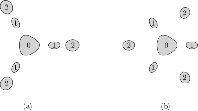
In this section we shall construct multipolar vortex equilibria in which a central patch is surrounded by satellite patches centered at the vertices of two nested regular -gons. The vertices of the polygons are either radially aligned with each other or out of phase by an angle , and the patches on each polygon are identical with the same strength; see Figure 3.
More precisely, we shall desingularize the following system of point vortices
| (4.1) |
with
| (4.2) |
where , and corresponds to the aligned configuration while refers to the staggered configuration. Assuming that and , one may easily check that the system of equations in (1.6) can be reduced to
| (4.3) |
where and
| (4.4) |
with . By symmetry arguments, one may easily check that
Thus, the identities in (4.4) become
| (4.5) |
Moreover, the differential of the mapping with respect to is given by
| (4.6) |
If the Jacobian determinant is non-trivial,
| (4.7) |
then the system (4.5) has a unique solution given by
| (4.8) |
In order to ensure that is non-vanishing, one has to assume that and verify the condition
| (4.9) |
Remark 4.1.
Remark 4.2.
While for general non-degenerate equilibria the differential was never onto, in this more symmetric setting the differential is onto whenever (4.7) holds. This will enable us to directly apply the implicit function theorem to the vortex patch equations, avoiding Lemma 2.6 and the use of integral identities.
4.1. Boundary equations
Let be a positive integer and , be three bounded simply connected domains containing the origin and contained in the ball . Assume in addition that is -fold symmetric, that is
| (4.10) |
and and are symmetric about the real axis. Given and and , with , we define the domains
| (4.11) | ||||
| (4.12) | ||||
| (4.13) |
where we recall that corresponds to the aligned configuration and refers to the staggered configuration. Let and consider the initial vorticity
| (4.14) |
Now assume that the evolution of is prescribed by the (2.9) with . While this initially gives equations, one for each patch, using the fact that
we shall show that this system can be reduced to a system of three equations, on the boundaries of and .
4.1.1. Euler equation
From (2.11) one has
| (4.15) |
where denotes a tangent vector to the boundary at the point and
In view of (4.12) and (4.13), the change of variables leads to
| (4.16) |
For any one has
In view of (4.10), making the change of variables in the first integral gives
| (4.17) |
From (4.12), (4.13) and (4.17) we conclude that if (4.15) is satisfied for , then it also satisfied for all . Thus, the system (4.15) is reduced to
| (4.18) |
We assume that the boundaries of the domains , in (4.12), (4.13) are parametrized by conformal mappings satisfying
Following the steps established in Section 2.2.1, more precisely (2.15), we may conclude that the dynamics the three boundaries is governed by the system
| (4.19) | ||||
| (4.20) |
for all and , where
| (4.21) | ||||
| (4.22) |
with the convention and
4.1.2. gSQG equations
| (4.23) |
where denotes a tangent vector to the boundary at the point and
for all . In view of (4.12) and (4.13), a suitable change of variables gives
Observe that for any one has
From (4.10), the change of variable in the first integral leads to
From the last identity and by (4.12) and (4.13), we conclude that the system (4.23) of equations can be reduced to a system of three equations,
Assume that the boundaries of the domains , in (4.12), (4.13) are parametrized by the conformal mappings satisfying
Then, from (2.27) one may conclude that the dynamics of three boundaries is described by
| (4.24) | ||||
| (4.25) |
for all and , where is defined in (2.25) and
| (4.26) | ||||
| (4.27) |
with the convention and
4.2. Existence of the nested polygonal vortex patch equilibria
For any we define the Banach spaces
| (4.28) |
where and are defined by
| (4.29) |
and and are given by (4.29). Note that if , the expansion of the associated conformal mapping is given by
which provides the -fold symmetry of the associated patch. We denote by the open unit ball in . Define the mapping
where , , is given by (4.1.2)–(4.25) for and by (4.19)–(4.20) for .
The proof of the existence of the co-rotating nested polygons follows from the next theorem, which gives the full statement of Theorem 1.9.
Theorem 4.3.
Let , such that satisfies (4.7), and let such that (4.9) holds. Then
-
(i)
There exists and a neighborhood of in such that can be extended to a mapping .
-
(ii)
where is given by (4.8).
-
(iii)
The linear operator is an isomorphism.
-
(iv)
There exists and a unique function such that
with and
(4.30) -
(v)
For all the domains , whose boundaries are given by the conformal parametrizations , are strictly convex.
Proof.
The regularity of the nonlinear operator follows from Proposition 2.2. In order to prove the reflection symmetry property we shall assume that the Fourier coefficients of are real, that is
| (4.31) |
and prove that
| (4.32) |
It is obvious that if satisfy (4.31), then
satisfies (4.32). Moreover, using (4.26) and (4.27), we check that the Fourier coefficients of and are also real for every satisfying (3.2), namely,
Then using (4.1.2) we conclude (4.32). Thus, it remains to check the -fold symmetry property of , namely, that if
| (4.33) |
then
| (4.34) |
We shall give the details of the proof in the case ; the case can be checked in a similar way. From (4.1.1) one has
Using the change of variables , we find
Then, by (4.33), we deduce that
In view of (4.22) and (4.33) we have
Summing over then gives
concluding the proof of (i). The proof of (ii) follows immediately from Proposition 2.2(ii), (4.5) and (4.8). In order to show (iii) we use Proposition 2.2(ii) and (4.6) to get, for all and ,
where is given by (2.32). Proposition 2.2(iv) and the assumption (4.7) then imply (iii).
The existence and uniqueness in (iv) follow form the implicit function theorem. In order to compute the asymptotic of the solution, we shall use the formula
| (4.35) |
For any with the expansion
with if is not a multiple of , we have
| (4.36) | ||||
where was calculated in (4.7). On the other hand, from (4.1.2)–(4.25) and (4.19)–(4.20) we have
| (4.37) |
with .
Case .
Case .
From (4.27) we have
with defined as for . Applying formula (2.23) gives
Inserting the last identity into (4.37) and then differentiating with respect , we obtain
Combining the two last identities with (4.35), (4.36) and (2.67), we get
where and are given by (4.30).
The convexity in (v) is established in exactly the same was as in the proof of Theorem 2.7. This ends the proof of the theorem. ∎
Acknowledgments
Miles H. Wheeler was partially supported by NSF-DMS grant 1400926. The work of Z. Hassainia is supported by Tamkeen under the NYU Abu Dhabi Research Institute grant of the center SITE.
References
- [1] Weiwei Ao, Juan Davila, Manuel del Pino, Monica Musso, and Juncheng Wei. Travelling and rotating solutions to the generalized inviscid surface quasi-geostrophic equation. Transactions of the American Mathematical Society, 374(374):6665–6689, 2021.
- [2] Hassan Aref. Vortex crystals. Advances in applied Mechanics, 39:2–81, 2003.
- [3] A. L. Bertozzi and P. Constantin. Global regularity for vortex patches. Comm. Math. Phys., 152(1):19–28, 1993.
- [4] Jacob Burbea. Motions of vortex patches. Lett. Math. Phys., 6(1):1–16, 1982.
- [5] Daomin Cao, Guolin Qin, Weicheng Zhan, and Changjun Zou. Existence and regularity of co-rotating and travelling global solutions for the generalized sqg equation. arXiv preprint arXiv:2103.03992, Mar 2021.
- [6] Daomin Cao, Guolin Qin, Weicheng Zhan, and Changjun Zou. Existence of co-rotating and travelling vortex patches with doubly connected components for active scalar equations. arXiv preprint arXiv:2103.04328, Mar 2021.
- [7] Angel Castro, Diego Córdoba, and Javier Gómez-Serrano. Existence and regularity of rotating global solutions for the generalized surface quasi-geostrophic equations. Duke Math. J., 165(5):935–984, 2016.
- [8] Angel Castro, Diego Córdoba, and Javier Gómez-Serrano. Uniformly rotating analytic global patch solutions for active scalars. Ann. PDE, 2(1):Art. 1, 34, 2016.
- [9] Angel Castro, Diego Córdoba, and Javier Gómez-Serrano. Uniformly rotating smooth solutions for the incompressible 2D Euler equations. Arch. Ration. Mech. Anal., 231(2):719–785, 2019.
- [10] M. Celli, E. A. Lacomba, and E. Pérez-Chavela. On polygonal relative equilibria in the -vortex problem. J. Math. Phys., 52(10):103101, 8, 2011.
- [11] Jean-Yves Chemin. Perfect incompressible fluids, volume 14 of Oxford Lecture Series in Mathematics and its Applications. The Clarendon Press, Oxford University Press, New York, 1998. Translated from the 1995 French original by Isabelle Gallagher and Dragos Iftimie.
- [12] Diego Córdoba, Marco A. Fontelos, Ana M. Mancho, and Jose L. Rodrigo. Evidence of singularities for a family of contour dynamics equations. Proc. Natl. Acad. Sci. USA, 102(17):5949–5952, 2005.
- [13] Darren G. Crowdy. Exact solutions for rotating vortex arrays with finite-area cores. J. Fluid Mech., 469:209–235, 2002.
- [14] Francisco de la Hoz, Zineb Hassainia, and Taoufik Hmidi. Doubly connected V-states for the generalized surface quasi-geostrophic equations. Arch. Ration. Mech. Anal., 220(3):1209–1281, 2016.
- [15] Francisco de la Hoz, Zineb Hassainia, Taoufik Hmidi, and Joan Mateu. An analytical and numerical study of steady patches in the disc. Anal. PDE, 9(7):1609–1670, 2016.
- [16] Francisco de la Hoz, Taoufik Hmidi, Joan Mateu, and Joan Verdera. Doubly connected -states for the planar Euler equations. SIAM J. Math. Anal., 48(3):1892–1928, 2016.
- [17] Gary S. Deem and Norman J. Zabusky. Vortex waves: Stationary ”-states,” interactions, recurrence, and breaking. Phys. Rev. Lett., 40:859–862, Mar 1978.
- [18] David G. Dritschel. A general theory for two-dimensional vortex interactions. J. Fluid Mech., 293:269–303, 1995.
- [19] L. E. Fraenkel. An introduction to maximum principles and symmetry in elliptic problems. Number 128. Cambridge University Press, 2000.
- [20] Francisco Gancedo. Existence for the -patch model and the QG sharp front in Sobolev spaces. Adv. Math., 217(6):2569–2598, 2008.
- [21] Claudia García. Kármán vortex street in incompressible fluid models. Nonlinearity, 33(4):1625–1676, 2020.
- [22] Claudia García. Vortex patches choreography for active scalar equations. Journal of Nonlinear Science, 31(5):1–31, 2021.
- [23] Claudia García and Susanna V. Haziot. Global bifurcation for corotating and counter-rotating vortex pairs, 2022.
- [24] Claudia García, Taoufik Hmidi, and Juan Soler. Non uniform rotating vortices and periodic orbits for the two-dimensional Euler equations. Arch. Ration. Mech. Anal., 238(2):929–1085, 2020.
- [25] Ludovic Godard-Cadillac, Philippe Gravejat, and Didier Smets. Co-rotating vortices with n fold symmetry for the inviscid surface quasi-geostrophic equation. arXiv preprint arXiv:2010.08194, 2020.
- [26] Javier Gómez-Serrano. On the existence of stationary patches. Adv. Math., 343:110–140, 2019.
- [27] Javier Gómez-Serrano, Jaemin Park, and Jia Shi. Existence of non-trivial non-concentrated compactly supported stationary solutions of the 2d euler equation with finite energy. arXiv preprint arXiv:2112.03821, 2021.
- [28] Javier Gómez-Serrano, Jaemin Park, Jia Shi, and Yao Yao. Symmetry in stationary and uniformly-rotating solutions of active scalar equations. Duke Mathematical Journal, 170(13):2957–3038, 2021.
- [29] Gustav Krichhoff. Vorlesungen über mathematische physik. Monatsh. Math. Phys., 8(1):A29–A29, 1897.
- [30] Zineb Hassainia and Taoufik Hmidi. On the V-states for the generalized quasi-geostrophic equations. Comm. Math. Phys., 337(1):321–377, 2015.
- [31] Zineb Hassainia and Taoufik Hmidi. Steady asymmetric vortex pairs for euler equations. Discrete Contin. Dyn. Syst., 41(4):1939–1969, 2021.
- [32] Zineb Hassainia, Nader Masmoudi, and Miles H. Wheeler. Global bifurcation of rotating vortex patches. Comm. Pure Appl. Math., 73(9):1933–1980, 2020.
- [33] Taoufik Hmidi. On the trivial solutions for the rotating patch model. J. Evol. Equ., 15(4):801–816, 2015.
- [34] Taoufik Hmidi and Joan Mateu. Bifurcation of rotating patches from Kirchhoff vortices. Discrete Contin. Dyn. Syst., 36(10):5401–5422, 2016.
- [35] Taoufik Hmidi and Joan Mateu. Degenerate bifurcation of the rotating patches. Adv. Math., 302:799–850, 2016.
- [36] Taoufik Hmidi and Joan Mateu. Existence of corotating and counter-rotating vortex pairs for active scalar equations. Comm. Math. Phys., 350(2):699–747, 2017.
- [37] Taoufik Hmidi, Joan Mateu, and Joan Verdera. Boundary regularity of rotating vortex patches. Arch. Ration. Mech. Anal., 209(1):171–208, 2013.
- [38] Taoufik Hmidi, Joan Mateu, and Joan Verdera. On rotating doubly connected vortices. J. Differential Equations, 258(4):1395–1429, 2015.
- [39] G. Keady. Asymptotic estimates for symmetric vortex streets. J. Austral. Math. Soc. Ser. B, 26(4):487–502, 1985.
- [40] Hansjörg Kielhöfer. Bifurcation theory, volume 156 of Applied Mathematical Sciences. Springer-Verlag, New York, 2004. An introduction with applications to PDEs.
- [41] Paul K. Newton. The -vortex problem, volume 145 of Applied Mathematical Sciences. Springer-Verlag, New York, 2001. Analytical techniques.
- [42] J. Norbury. Steady planar vortex pairs in an ideal fluid. Comm. Pure Appl. Math., 28(6):679–700, 1975.
- [43] Kevin Anthony O’Neil. Stationary configurations of point vortices. Trans. Amer. Math. Soc., 302(2):383–425, 1987.
- [44] Edward A. Overman, II. Steady-state solutions of the Euler equations in two dimensions. II. Local analysis of limiting -states. SIAM J. Appl. Math., 46(5):765–800, 1986.
- [45] R. T. Pierrehumbert. A family of steady, translating vortex pairs with distributed vorticity. Journal of Fluid Mechanics, 99(1):129–144, 1980.
- [46] Coralie Renault. Relative equilibria with holes for the surface quasi-geostrophic equations. J. Differential Equations, 263(1):567–614, 2017.
- [47] José Luis Rodrigo. On the evolution of sharp fronts for the quasi-geostrophic equation. Comm. Pure Appl. Math., 58(6):821–866, 2005.
- [48] Matthew Rosenzweig. Justification of the point vortex approximation for modified surface quasi-geostrophic equations. SIAM J. Math. Anal., 52(2):1690–1728, 2020.
- [49] P. G. Saffman. Vortex dynamics. Cambridge Monographs on Mechanics and Applied Mathematics. Cambridge University Press, New York, 1992.
- [50] P. G. Saffman and R. Szeto. Equilibrium shapes of a pair of equal uniform vortices. Phys. Fluids, 23(12):2339–2342, 1980.
- [51] Bruce Turkington. Corotating steady vortex flows with -fold symmetry. Nonlinear Anal., 9(4):351–369, 1985.
- [52] Yieh Hei Wan. Desingularizations of systems of point vortices. Phys. D, 32(2):277–295, 1988.
- [53] B. B. Xue, E. R. Johnson, and N. R. McDonald. New families of vortex patch equilibria for the two-dimensional euler equations. Physics of Fluids, 29(12):123602, 2017.
- [54] Victor Iosifovich Yudovich. Non-stationary flows of an ideal incompressible fluid. Zhurnal Vychislitel’noi Matematiki i Matematicheskoi Fiziki, 3(6):1032–1066, 1963.
Department of Mathematics,
New York University in Abu Dhabi,
Saadiyat Island,
P.O. Box 129188,
Abu Dhabi,
United Arab Emirates
,
E-mail address: zh14@nyu.edu
Department of Mathematical Sciences,
University of Bath,
Bath BA2 7AY, UK,
E-mail address: mw2319@bath.ac.uk