Modelling the Multiwavelength Variability of Mrk 335  using Gaussian Processes

Abstract

The optical and UV variability of the majority of AGN may be related to the reprocessing of rapidly-changing X-ray emission from a more compact region near the central black hole. Such a reprocessing model would be characterised by lags between X-ray and optical/UV emission due to differences in light travel time. Observationally however, such lag features have been difficult to detect due to gaps in the lightcurves introduced through factors such as source visibility or limited telescope time. In this work, Gaussian process regression is employed to interpolate the gaps in the Swift X-ray and UV lightcurves of the narrow-line Seyfert 1 galaxy Mrk 335. In a simulation study of five commonly-employed analytic Gaussian process kernels, we conclude that the Matern $\frac{1}{2}$ and rational quadratic kernels yield the most well-specified models for the X-ray and UVW2 bands of Mrk 335. In analysing the structure functions of the Gaussian process lightcurves, we obtain a broken power law with a break point at 125 days in the UVW2 band. In the X-ray band, the structure function of the Gaussian process lightcurve is consistent with a power law in the case of the rational quadratic kernel whilst a broken power law with a break point at 66 days is obtained from the Matern $\frac{1}{2}$ kernel. The subsequent cross-correlation analysis is consistent with previous studies and furthermore, shows tentative evidence for a broad X-ray-UV lag feature of up to 30 days in the lag-frequency spectrum where the significance of the lag depends on the choice of Gaussian process kernel.

1 Introduction

Active galactic nuclei (AGN) show strong and variable emission across multiple wavelengths. The UV emission from an AGN is believed to be dominated by thermal emission from an accretion disc close to the central super-massive black hole (SMBH, e.g. Pringle, 1981). The variability of optical and UV AGN emission is stochastic and described by random Gaussian fluctuations (e.g. Welsh et al., 2011; Gezari et al., 2013; Zhu et al., 2016; Sánchez-Sáez et al., 2018; Smith et al., 2018; Xin et al., 2020) with the autocorrelation functions of such fluctuations adhering to the ‘damped random walk’ model. The X-ray emission from an AGN is often found to show faster variability relative to emission at longer wavelengths (e.g. Mushotzky et al., 1993; Gaskell and Klimek, 2003) and originates from a more compact region (e.g. Morgan et al., 2008; Chartas et al., 2017).

The relationship between the UV and X-ray emission has been well studied. For instance, correlations between the variability in two energy bands has been seen in some individual sources (e.g. Shemmer et al., 2001; Buisson et al., 2017) while others do not show significant evidence for similar correlation (e.g. Smith and Vaughan, 2007; Buisson et al., 2018). In sources where correlation is found, lags that are related to the light travel time between two emission regions are frequently observed. These lags are often found to be on timescales of days and are longer than those predicted by classical disc theories (Shakura and Sunyaev, 1973). Such lag amplitudes indicate a disc of size a few times larger than expected (e.g. Edelson et al., 2000; Shappee et al., 2014; Troyer et al., 2016; Buisson et al., 2017). Alternatively, some modified models have been proposed for the underestimation of lags by the classical thin disc model, e.g. disc turbulence (e.g. Cai et al., 2020), additional varying FUV illumination (e.g. Gardner and Done, 2017), a tilted or inhomogeneous inner disc (e.g. Dexter and Fragile, 2011; Starkey et al., 2017) or an extended coronal region (e.g. Kammoun et al., 2021). Much shorter lags, e.g. hundreds of seconds, in agreement with the Shakura and Sunyaev (1973) model have been rarely observed by comparison (e.g. in NGC 4395, McHardy et al., 2016).

The Neil Gehrels Swift Observatory has been monitoring the X-ray sky in the past decade in tandem with simultaneous pointings in the optical and UV band. In this work, we focus on the X-ray and UVW2 ($\lambda=$212 nm) lightcurves of the narrow-line Seyfert 1 galaxy (NLS1, e.g. Gallo, 2018) Mrk 335 obtained by XRT and UVOT, the soft X-ray and UV/optical telescopes on Swift. Mrk 335 was one of the brightest X-ray sources prior to 2007, before its flux diminished by $10-50\times$ its original brightness (Grupe et al., 2007). The X-ray brightness has not recovered since. During this low X-ray flux period, the UV brightness remains relatively unchanged rendering Mrk 335 X-ray weak (Tripathi et al., 2020). The behavior has been explained as a possible collapse of the X-ray corona e.g. (Gallo et al., 2013, 2015; Parker et al., 2014) and/or increased absorption in the X-ray emitting region e.g. (Grupe et al., 2012; Longinotti et al., 2013, 2019; Parker et al., 2019).

Mrk 335 has been continuously monitored since 2007 making it one of the best-studied AGN with Swift. Previous studies from the Swift monitoring program can be found in Grupe et al. (2007, 2012); Gallo et al. (2018); Tripathi et al. (2020); Komossa et al. (2020). The X-rays are constantly fluctuating and regularly display large amplitude flaring e.g. Wilkins et al. (2015). The UV are significantly variable, but at a much smaller amplitude than the X-rays. Gallo et al. (2018) found tentative evidence for lags of $\approx 20$ days based on cross-correlation analyses, suggesting a potential reprocessing mechanism of the more variable X-ray emission in the UV emitter of this source. One challenge faced by the Swift monitoring program is that the lightcurves are not continuously sampled and hence standard Fourier techniques cannot be applied. This uneven sampling of the lightcurves is imposed by limited telescope time.

In the context of cross-correlation analysis, methods have been developed to address the problem of unevenly-sampled lightcurves. In Reynolds (2000), the method of Press et al. (1992) is extended to interpolate the lightcurve gaps using a model of the covariance function, or equivalently the power spectrum, of the lightcurve. In Bond et al. (1998); Miller et al. (2010); Zoghbi et al. (2013) a maximum likelihood approach is taken to fit models of the lightcurve power spectra which accounts for the correlation between the lightcurves. In this paper we focus on a relatively new approach to tackle unevenly-sampled lightcurves.

Gaussian processes confer a Bayesian nonparametric framework to model general time series data (Roberts et al., 2013; Tobar et al., 2015) and have proven effective in tasks such as periodicity detection (Durrande et al., 2016) and spectral density estimation (Tobar, 2018). More broadly Gaussian processes have recently demonstrated modelling success across a wide range of spatial and temporal application domains including robotics (Deisenroth and Rasmussen, 2011; Greeff and Schoellig, 2020), Bayesian optimisation (Shahriari et al., 2015; Grosnit et al., 2020; Cowen-Rivers et al., 2021; Grosnit et al., 2021) as well as areas of the natural sciences such as molecular machine learning (Nigam et al., 2021; Griffiths and Hernández-Lobato, 2020; Moss and Griffiths, 2020; Thawani et al., 2020; Griffiths et al., 2019; Hase et al., 2020; Bartók et al., 2010), genetics (Moss et al., 2020) and materials science (Cheng et al., 2020; Zhang et al., 2020). In the context of astrophysics there is a recent trend favouring nonparametric models such as Gaussian processes due to the flexiblity afforded when specifying the underlying data modelling assumptions. Applications have arisen in lightcurve modelling (Luger, Foreman-Mackey, Hedges and Hogg, 2021; Luger, Foreman-Mackey and Hedges, 2021a, b), continuous-time autoregressive moving average (CARMA) processes Yu and Richards (2021), modelling stellar activity signals in radial velocity data (Rajpaul et al., 2015), lightcurve detrending (Aigrain et al., 2016), learning imbalances for variable star classification (Lyon et al., 2020), inferring stellar rotation periods (Angus et al., 2018), estimating the dayside temperatures of hot Jupiters (Pass et al., 2019), exoplanet detection (Jones et al., 2017; Czekala et al., 2017; Gordon et al., 2020; Langellier et al., 2021), spectral modelling (Gibson et al., 2012; Nikolov et al., 2018; Diamond-Lowe et al., 2020) as well as blazar variability studies (Karamanavis, 2015, 2017; Covino et al., 2020; Yang et al., 2021).

It has recently been demonstrated in lightcurve simulations by Wilkins (2019) that a Gaussian process framework can compute time lags associated with X-ray reverberation from the accretion disc that are longer and observed at lower frequencies than can be measured by applying standard Fourier transform techniques to the longest available continuous segments. It is for this principal reason that we choose to employ Gaussian processes for our timing analysis. Further desirable facets of Gaussian processes include the fact that, unlike parametric models, they do not make strong assumptions about the shape of the underlying light curve (Wang et al., 2012). Additionally, we may perform Bayesian model selection at the level of the covariance function or kernel allowing us to quantitatively compare different models of the lightcurve power spectrum. Finally in the cross-correlation analysis, we may make a weaker modelling assumption than (Zoghbi et al., 2013) in treating the X-ray and UV lightcurves as being independent (Wilkins, 2019).

The paper is outlined as follows: In section 2, we provide background on Gaussian processes including discussion of different kernels as well as Bayesian model selection, the criterion used to choose between kernels. In section 3 we describe the procedures used to fit Gaussian processes to the X-ray and UVW2 bands including aspects such as identification of the flux distribution, consideration of measurement noise as well as a simulation study to determine the appropriate kernels. In section 4 we compare the structure functions of the gp-interpolated lightcurves with the observational structure functions from Gallo et al. (2018). In section 5 we present a cross-correlation analysis of the X-ray and UVW2 bands using the gp-interpolated lightcurves. Finally, in section 6 we provide concluding remarks about the discrepancy between the observational and gp-derived structure functions as well as the implications of the cross-correlation analysis, namely that the broad lag features suggest an extended emission region of the disc in Mrk 335 during the reverberation process. All code for reproducing the analysis is available at https://github.com/Ryan-Rhys/Mrk_335.

2 Gaussian Processes

We may define a Gaussian process (gp) as a collection of random variables, any finite number of which have a joint Gaussian distribution. When the gp is used as a prior over functions, the aforementioned random variables consist of function values $f(t)$ at different points in time $t$. In our setting $f$ represents flux or count rate. The gp is characterised by a mean function

$$m(t)=\mathbb{E}[f(t)]$$ (1)

and a covariance function

$$k(t,t^{\prime})=\mathbb{E}[(f(t)-m(t))(f(t^{\prime})-m(t))].$$ (2)

The process is written as follows

$$f(t)\sim\mathcal{GP}\big{(}m(t),k(t,t^{\prime})\big{)}.$$ (3)

The mean function is set to the empirical mean of the standardised observational data in the cases we consider. Standardisation, in this case refers to the common practice of subtracting the mean and dividing by the standard deviation of the data when fitting the gp in order to facilitate the identification of appropriate hyperparameters (Murray, 2008). The standardisation is reversed once the fitting procedure is complete in order to obtain predictions on the original scale of the data. $m(t)=0$ will be assumed henceforth for the sake of the current presentation. The covariance function computes the pairwise covariance between two random variables (function values). In the gp literature, the covariance function is commonly referred to as the kernel and is denoted as

$$k(t,t^{\prime})=\text{cov}\big{(}f(t),f(t^{\prime})\big{)}.$$ (4)

Informally, the kernel is responsible for determining the smoothness of the functions which the gp is capable of fitting. The inductive bias created by the choice of kernel is an important consideration in Gaussian process modelling.

2.1 Kernels

The most widely-known kernel is the squared exponential (SE) or radial basis function (RBF) kernel

$$k_{\text{SQE}}(t,t^{\prime})=\sigma_{f}^{2}\exp\bigg{(}\frac{-|t-t^{\prime}|^{2}}{2\ell^{2}}\bigg{)},$$ (5)

where $\sigma_{f}^{2}$ is the signal amplitude hyperparameter (vertical lengthscale) and $\ell$ is the (horizontal) lengthscale hyperparameter. For such hyperparameters, we will adopt the notation of $\theta$ to represent the set of kernel hyperparameters. It has been argued by Stein (2012) that the smoothness assumptions of the squared exponential kernel are unrealistic for many physical processes. As such, kernels such as the Matern

$$k_{\text{Matern}}(t,t^{\prime})=\frac{2^{1-\nu}}{\Gamma(\nu)}\bigg{(}\frac{\sqrt{2\nu}-|t-t^{\prime}|}{\ell}\bigg{)}^{\nu}K_{\nu}\bigg{(}\frac{\sqrt{2\nu}-|t-t^{\prime}|}{\ell}\bigg{)},$$ (6)

are more commonly seen in the machine learning literature. Here $K_{\nu}$ is a modified Bessel function of the second kind, $\Gamma$ is the gamma function and $\nu$ is a non-negative parameter of the kernel which is typically taken to be either $\frac{3}{2}$ or $\frac{5}{2}$ (Rasmussen and Williams, 2006). The lengthscale hyperparameter $\ell$ can be thought of loosely as a decay coefficient for the covariance between inputs as they become increasingly far apart in the input space; the further apart the inputs are, the less correlated they will be. The final kernel used in this work is the rational quadratic (RQ) kernel

$$k_{RQ}(t,t^{\prime})=\bigg{(}1+\frac{|t-t^{\prime}|^{2}}{2\alpha\ell^{2}}\bigg{)}^{-\alpha}.$$ (7)

where $\alpha,\ell>0$. The rational quadratic kernel can be viewed as a scale mixture of squared exponential kernels with different characteristic lengthscales. All kernels used in this work are stationary kernels and as such it should be stated that this reflects a modelling assumption that the underlying time series is stationary. The extension of the current work to include non-stationary kernels will be discussed in section 6.

2.2 Prediction with Gaussian Processes

To illustrate the homoscedastic (constant noise) gp predictive model we use X-ray timing as an example. We wish to model the count rate $f(t)$. We place a Gaussian process prior over $f$,

$$p(\mathbf{f}(\mathbf{t})|\theta)=\mathcal{GP}\big{(}0,K(\mathbf{t},\mathbf{t})\big{)}$$ (8)

where $\mathbf{f}$ denotes the vector of function values evaluated at the set of times $\{t_{i}\}_{i=1}^{N},N\in\mathbb{N}$. $K(\mathbf{t},\mathbf{t})$ is a kernel matrix where entries are computed by the kernel function as $[K]_{ij}=k(t_{i},t_{j})$. $\theta$ represents the set of kernel hyperparameters. The Gaussian process prior is written as

$$p(\mathbf{y}(\mathbf{t})|\theta)=\mathcal{GP}\big{(}0,K(\mathbf{t},\mathbf{t})+I\sigma_{y}^{2}\big{)},$$ (9)

where $I\sigma_{y}^{2}$ represents the variance of iid Gaussian noise on the observations $\mathbf{y}$. The applicability of such a noise model, also known as a Gaussian likelihood, will be discussed further in subsection 3.2. Once we have observed some data $\mathbf{y}$, the joint distribution over the observed data $\mathbf{y}$ and the predicted function values $\mathbf{f}*$ at test locations $\textbf{t}*$ may be written as

$$\begin{bmatrix}\mathbf{y}\\ \mathbf{f_{*}}\\ \end{bmatrix}\sim\mathcal{N}\bigg{(}0,\begin{bmatrix}K(\mathbf{t},\mathbf{t})+\sigma_{y}^{2}I&K(\mathbf{t},\mathbf{t_{*}})\>\\ K(\mathbf{t_{*}},\mathbf{t})\phantom{+\>\>\sigma{y}^{2}}&K(\mathbf{t_{*}},\mathbf{t_{*}})\end{bmatrix}\bigg{)},$$ (10)

where $\mathcal{N}$ is the multivariate Gaussian probability density function. The joint prior may be conditioned on the observations through

$$p(\mathbf{f_{*}}|\mathbf{y})=\frac{p(\mathbf{f_{*}},\mathbf{y})}{p(\mathbf{y})}$$ (11)

which enforces that the joint prior agrees with the observed target values $\mathbf{y}$. The predictive distribution is thus given as

$$p(\mathbf{f_{*}}|\mathbf{t},\mathbf{y},\mathbf{t_{*}})=\mathcal{N}\big{(}\mathbf{\bar{f}_{*}},\text{cov}(\mathbf{f_{*}})\big{)}$$ (12)

with the predictive mean at test locations $\mathbf{t_{*}}$ being

$$\mathbf{\bar{f_{*}}}=K(\mathbf{t_{*}},\mathbf{t})[K(\mathbf{t},\mathbf{t})+\sigma_{y}^{2}I]^{-1}\mathbf{y}$$ (13)

and the predictive uncertainty being

$$\text{cov}(\mathbf{f_{*}})=K(\mathbf{t_{*}},\mathbf{t_{*}})-K(\mathbf{t_{*}},\mathbf{t})[K(\mathbf{t},\mathbf{t})+\sigma_{y}^{2}I]^{-1}K(\mathbf{t},\mathbf{t_{*}}).$$ (14)

Analysing the form of this expression one may notice that the first term $K(\mathbf{t_{*}},\mathbf{t_{*}})$ in the expression for the predictive uncertainty $\text{cov}(\mathbf{f}*)$ may be viewed as the prior uncertainty and the second term $K(\mathbf{t_{*}},\mathbf{t})[K(\mathbf{t},\mathbf{t})+\sigma_{y}^{2}I]^{-1}K(\mathbf{t},\mathbf{t_{*}})$ can be thought of as a subtractive factor that accounts for the reduction in uncertainty when observing the data points $\mathbf{y}$.

2.3 Bayesian Model Selection

One desirable property of Gaussian processes and Bayesian models in general is the ability to carry out hierarchical modelling (MacKay, 1992; van der Wilk, 2019). The three tiers of the modelling hierarchy are:

1. Model Parameters

2. Model Hyperparameters

3. Model Structures

In the case of the nonparametric Gaussian process framework, parameters do not have the same meaning as in parametric Bayesian models and are instead obtained from the posterior distribution over functions. Hyperparameters are typically parameters of the kernel function such as signal amplitudes and lengthscales. An important entity for hyperparameter optimisation in Gaussian processes is the log marginal likelihood or evidence (MacKay, 1991)

$$\log p(\mathbf{y}|\mathbf{t},\theta)= \underbrace{-\frac{1}{2}\mathbf{y}^{\top}(K_{\theta}(\mathbf{t},\mathbf{t})+\sigma_{y}^{2}I)^{-1}\mathbf{y}}_{\text{encourages fit with data}}$$ (15)

$$\underbrace{-\frac{1}{2}\log|K_{\theta}(\mathbf{t},\mathbf{t})+\sigma_{y}^{2}I|}_{\text{controls model capacity}}-\frac{N}{2}\log(2\pi).$$

Where $N$ is the number of observations and the subscript notation on the kernel matrix $K_{\theta}(\mathbf{t},\mathbf{t})$ is chosen to indicate the dependence on the set of hyperparameters $\theta$. The two terms in the expression for the marginal likelihood embody Occam’s Razor (Rasmussen and Ghahramani, 2001) in their preference for selecting models of intermediate capacity. The first term in Equation 15 acts as a term that penalises functions that do not fit the data well whereas the second term acts like a regulariser, disfavouring overly complex models. In this work kernel hyperparameters are chosen to optimise the marginal likelihood. At the level of model structures, the fit achieved by different kernels can be quantitatively assessed by comparing the values of the optimised log marginal likelihood objective.

3 Gaussian Process Modelling of Mrk 335

In this paper we consider the Swift X-ray and UVW2 lightcurves in time bins of one day. We refer the reader to Gallo et al. (2018) for details of the data reduction processes. The observational measurements used in this work run from $54327-58626$ modified Julian days and comprise $509$ data points for the X-ray band and $498$ data points for the UVW2 band. We consider the latest UVOT sensitivity calibration file (‘swusenscorr20041120v006.fits’) to account for the sensitivity loss with time in the UVW2 band.

3.1 Identifying the Flux Distribution

In order to assess the applicability of Gaussian processes in modelling the flux distribution of the X-ray and UVW2 bands of Mrk 335, we perform a series of graphical distribution tests to determine the sample distribution. The histograms of the log count rates for the X-ray, and flux for the UV bands, of Mrk 335 are shown in Figure 1. The histograms show that the distribution of the UVW2 flux is approximately Gaussian-distributed whereas the X-ray count rate distribution appears to be log-Gaussian distributed in line with the general observation of Uttley and McHardy (2005) that fluxes from accreting black holes tend to follow log-Gaussian distributions. We provide further graphical distribution tests based on probability-probability (PP) plots and empirical cumulative distribution functions (ECDFs) in Appendix A.

Furthermore, following Wilkins (2019) we perform a Kolmogorov-Smirnov test for goodness-of-fit where the null hypothesis is that the sample was drawn from a Gaussian distribution. For the UVW2 flux values we obtain a p-value of $0.164$. We obtain a p-value of $1.017e^{-20}$ for the raw X-ray count rates and a p-value of $0.028$ for the log-transformed X-ray count rates. As such, we cannot reject the null hypothesis that either UVW2 flux or log-transformed X-ray count rates are drawn from a Gaussian distribution at the $1\%$ level of significance. We may however reject the null hypothesis in the case of the raw X-ray count rates, providing evidence that the raw X-ray count rates should be log-transformed in order to be well-modelled by a Gaussian distribution. As such, we log transform the raw X-ray count rates and leave the UVW2 flux values unchanged.

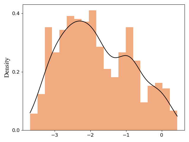
(a) X-Ray Log Count Rates

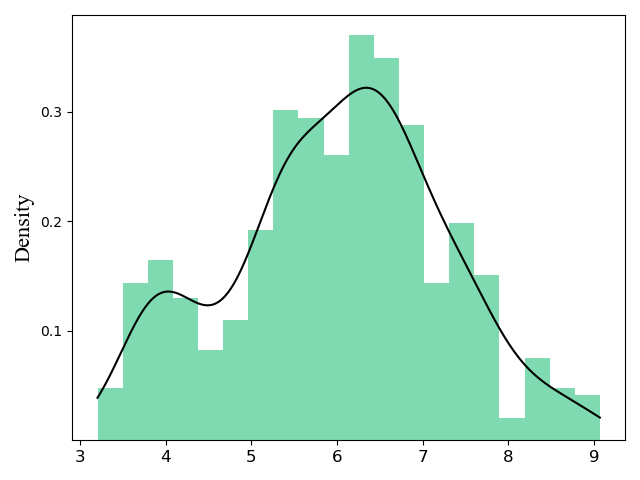
(b) UVW2 Flux

Figure 1: Histograms of the observed Swift X-ray log count rate and UVW2 flux overlaid with Gaussian kernel density estimates. The raw UVW2 flux values have been scaled by $1e^{14}$.

3.2 Noise

As noted by Wilkins (2019) fitting a Gaussian process to the logarithm of the count rate is appropriate only in the limit of a large signal-to-noise ratio. In the case of Mrk 335, the Poisson (shot) noise intrinsic to the photon detectors used to obtain the flux measurements is over an order of magnitude smaller than the flux measurement itself. As such the choice of the log-Gaussian process would appear to be justified.

3.3 Simulations

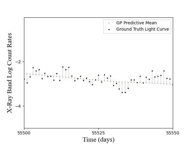
Figure 2: Residual plot. The normalised RSS metric is the sum of squared residuals divided by the total number of discretised points (4390) comprising the simulated lightcurve. A residual in this case represents the difference between the Gaussian process predictive mean and the ground truth value of the simulated lightcurve.

We undertake a simulation study in order to quantitatively assess the abilities of different kernels to interpolate gapped simulated lightcurves. Observational power spectral densities (PSDs) of AGN are well-described by (broken) power laws (Mchardy et al., 2004). As such, our simulations employ a power law PSD with index fit to the observational data. Our goals with the study are twofold: Firstly, although we cannot be sure of the true PSD for the observational data, we hope that the simulations may afford a good proxy for identifying performant kernels based on the fact that AGN typically exhibit power law-like PSDs and secondly, we wish to test whether a kernel’s ability to reconstruct the full simulated lightcurve correlates with its marginal likelihood value for the gapped data on which it is trained. If there is a correlation, we may use the marginal likelihood as a metric for identifying the appropriate kernel on the observational data.

One thousand simulated light curves with gaps are generated for the Mrk 335  X-ray and UV bands using the method of Davies and Harte (1987), first applied in astrophysics by Timmer and König (1995). For each lightcurve we have access to the ground truth functional form of the lightcurve before the introduction of gaps. Computationally, the ground truth lightcurve is evaluated on a fine, discrete grid of $4390$ time points whereas the gapped lightcurves are evaluated on a coarser, unevenly-spaced grid of $498$ time points for the UV simulations and $509$ time points for the X-ray simulations in line with the number of observational data points. We then quantify how well each gp kernel performs in recovering the ground truth lightcurve by measuring the normalised residual sum of squared errors,

$$\text{RSS}=\frac{1}{N}\sum_{i=1}^{N}(f(t_{i})-y_{i})^{2}$$ (16)

where $f(t_{i})$ is the Gaussian process prediction at grid point $t_{i}$ and $y_{i}$ is the true simulated count rate value. The RSS values are averaged over the one thousand simulated lightcurves. We provide an illustration of the RSS metric in Figure 2. In addition, we compute the averaged negative log marginal likelihood (NLML) for each kernel:

$$\text{NLML}=\frac{1}{2}\mathbf{y}^{\top}(K_{\theta}(\mathbf{t},\mathbf{t})+\sigma_{y}^{2}I)^{-1}+\mathbf{y}\frac{1}{2}\log|K_{\theta}(\mathbf{t},\mathbf{t})+\sigma_{y}^{2}I|+\frac{N}{2}\log(2\pi).$$ (17)

The NLML in this case is the negative of the quantity given in Equation 15. Kernel hyperparameters were selected via optimisation of the NLML using the scipy optimiser of GPflow (Matthews et al., 2017). The jitter level was fixed at 0.001, a small positive number to ensure numerical stability. The output values (flux or the logarithm of the count rate) were standardised according to their empirical mean and standard deviation. We use a constant mean function set to the empirical mean of the data following standardisation as discussed in section 2.

We report the results of this simulation study in Table 1. The NLML values show correlation with RSS, thus providing evidence that NLML is an appropriate metric for determining the Gaussian process kernel for the real observational data (for which the ground truth lightcurve is of course not available). A paired t-test was conducted to determine whether the RSS results were significant in terms of identifying the best kernel. For the X-ray simulations, a t-statistic of $9$ was obtained corresponding to a two-sided p-value of $5^{-20}$. For the UVW2 simulations, a t-statistic of $-22$ was obtained corresponding to a two-sided p-value of $9^{-85}$. As such, the null hypothesis that the performance discrepancy between kernels on the RSS metric is due to chance variation across $1000$ simulations, may be rejected at the $1\%$ level of significance. We offer further rationalisation in Appendix B for why the top two performing kernels in the simulation study are the Matern $\frac{1}{2}$ and rational quadratic kernels.

Table 1: Performance comparison of kernels based on the NLML on the simulated gapped X-ray and UV lightcurves and normalised residual sum of squared errors (RSS) on the ground truth simulated lightcurves. The mean NLML and RSS across 1000 simulations are reported with the standard error. UVW2 RSS values have an exponent of $-30$. Bold values indicate best performance.

Kernel	NLML	RSS
X-Ray
Matern$\frac{1}{2}$	$\textbf{180.2}\pm\>\textbf{3.8}$	$0.121\pm\>0.002$
Matern$\frac{3}{2}$	$420.7\pm\>3.3$	$0.309\pm\>0.003$
Matern$\frac{5}{2}$	$523.5\pm\>2.9$	$0.374\pm\>0.003$
Rational Quadratic	$\textbf{184.2}\pm\>\textbf{3.6}$	$\textbf{0.117}\pm\>\textbf{0.002}$
Squared Exponential	$632.1\pm\>1.5$	$0.554\pm\>0.004$
UVW2
Matern$\frac{1}{2}$	$\textbf{-399.0}\pm\>\textbf{5.2}$	$\textbf{2.9}\pm\>\textbf{0.08}$
Matern$\frac{3}{2}$	$-298.3\pm\>6.0$	$7.9\pm\>0.25$
Matern$\frac{5}{2}$	$-219.6\pm\>6.5$	$17.0\pm\>0.41$
Rational Quadratic	$-349.2\pm\>5.4$	$3.4\pm\>0.09$
Squared Exponential	$-65.0\pm\>7.4$	$32.8\pm\>0.55$

3.4 Gaussian Process Fits

The fits to the observational data for the UVW2 and X-ray bands are shown in 3(d) and 4(d) respectively. In an analogous fashion to the simulation experiments we evaluate five stationary kernels: Matern $\frac{1}{2}$, Matern $\frac{3}{2}$, Matern $\frac{5}{2}$, rational quadratic and squared exponential. We choose to display the two kernels, rational quadratic and Matern $\frac{1}{2}$ which performed best in the simulation study in their abilities to model power law-like PSDs. These kernels also have the most favourable values under the NLML metric for the observational data. We again use a constant mean function set to the empirical mean of the data following standardisation. We optimise all kernel hyperparameters under the marginal likelihood save for the noise level which we fix to a constant value in the standardised space. This constant noise value is computed by dividing the mean output value in the standardised space by the mean signal-to-noise ratio in the original space.

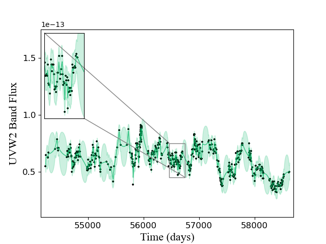
(a) UV Band — Matern $\frac{1}{2}$ — Mean.

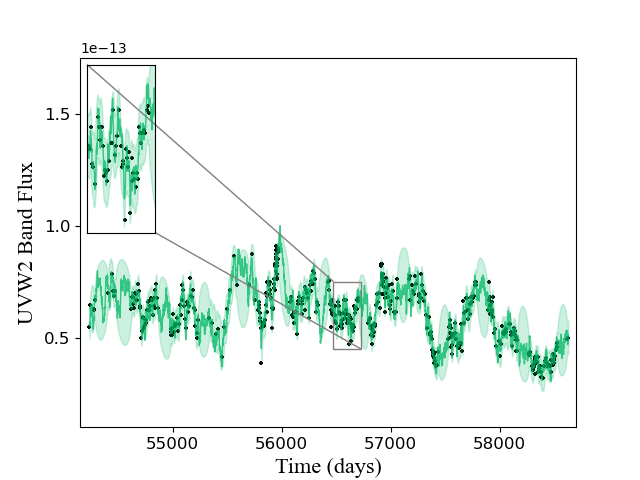
(b) UV Band — Matern $\frac{1}{2}$ — Sample.

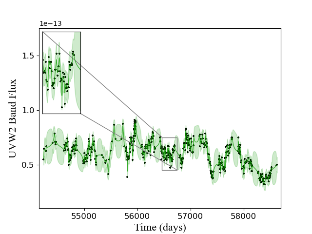
(c) UV Band — Rational Quadratic — Mean.

(d) UV Band — Rational Quadratic — Sample

Figure 3: gp lightcurves for the UVW2 band. The shaded regions denote the gp 95% confidence interval.

We show both the gp mean and a sample from the gp posterior in separate plots. The insets are included to highlight the variability of the fit.

(a) X-ray Band — Matern $\frac{1}{2}$ — Mean.

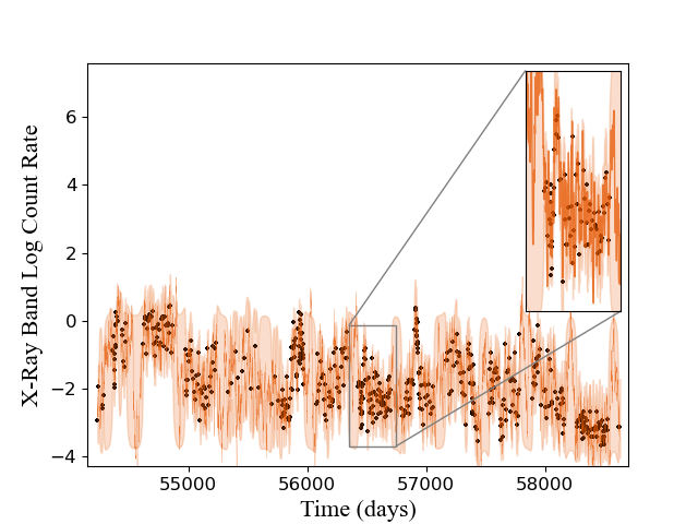
(b) X-ray Band — Matern $\frac{1}{2}$ — Sample.

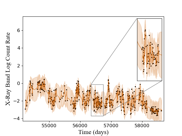
(c) X-ray Band — Rational Quadratic — Mean.

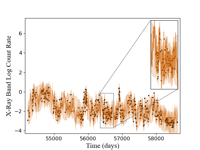
(d) X-ray Band — Rational Quadratic — Sample

Figure 4: gp lightcurves for the X-ray band. The shaded regions denote the gp 95% confidence interval.

We show both the gp mean and a sample from the gp posterior in separate plots. The insets are included to highlight the variability of the fit.

4 Structure Function Analysis

Ideally we would like to examine the PSD of the Gaussian process fits to the observational data. The PSD characterises the distribution of power over frequencies of a given emission band and properties of the PSD can be linked to underlying physical processes in the accretion disk. Computation of the PSD, while possible, can be complicated by the uneven sampling of the observational data, leading previous studies to instead perform a structure function analysis on the Mrk 335  data (Gallo et al., 2018). While it is possible to extract the PSD from the learned kernel (Wilkins, 2019), in this work we choose to perform a structure function analysis of the gp lightcurves in order to compare directly against the results of Gallo et al. (2018). We follow the method described in Simonetti et al. (1985); Hughes et al. (1992); di Clemente et al. (1996); Collier and Peterson (2001); Gallo et al. (2018). The binned structure function is defined as:

$$\text{SF}(\tau)=\frac{1}{N(\tau)}\sum_{i}\>[f(t_{i})-f(t_{i}+\tau)]^{2}$$ (18)

where $\tau=t_{j}-t_{i}$ is the distance between pairs of points $i$ and $j$ such that $t_{j}>t_{i}$. The structure function is binned according to $\tau$ where the centres of each bin are given by $\tau_{i}=(i-\frac{1}{2})\delta$. $\delta$ in this instance is the structure function resolution. We use the same $\delta$ as in Gallo et al. (2018), namely 5.3 days for the structure function computation over both the X-ray and UVW2 bands. $f(t_{i})$ gives the count rate value at time point $t_{i}$ and $N(\tau)$ is the number of structure function pairs in each bin $i$ with centre $\tau_{i}$. Accounting for measurement noise by subtracting twice the mean noise variance from each structure function bin, as performed in Gallo et al. (2018) was found to have negligible effect on the gp structure functions and so we ignore it. As in Gallo et al. (2018), we normalise the structure function values by the global lightcurve variance.

The gp structure functions for the interpolated lightcurves are shown in Figure 5. The $1\sigma$ gp error bars are obtained by computing the structure function over 50 samples from the Gaussian process posterior. Each sample gives rise to highly similar structure functions and so the errors are not visible on the plot. The structure functions computed from the observational data, 509 and 498 data points for the X-ray and UV bands of Mrk 335  respectively, are included for reference. In contrast to the gp structure function errorbars, in the case of the observational data the error bars are computed as $\frac{\sigma_{i}}{\sqrt{(}\frac{N_{i}}{2})}$ where $\sigma_{i}$ is the noise standard deviation in bin $i$ and $N_{i}$ is the number of pairs in bin $i$.

The Gaussian process structure functions are compared against the observational structure functions in Figure 5. In addition, we plot broken power law fits to the gp structure functions, the parameters of which are given in Table 2. In the UVW2 band, both Gaussian process kernels yield structure functions possessing a consistent break point at ca. 125 days. In the X-ray band the Matern $\frac{1}{2}$ kernel yields a break point at 66 days whereas the rational quadratic kernel fit yields an unbroken power law. Given the discrepancy between gp kernels, we do not find definite evidence for a break in the X-ray power law.

Of particular interest is whether the dip in the X-ray structure function is an expected feature of the latent lightcurve or a measurement artefact arising from uneven sampling. In order to assess the potential for the dip to be a sampling artefact, we perform simulations using the Timmer and Konig algorithm from subsection 3.3. In this case we compute structure functions of gapped lightcurves and compare against structure functions derived from the ground truth lightcurves with no gaps. One representative simulation is depicted in Figure 6. In this instance a similar dip to that found in the observational data is observed in the X-ray band simulation. This highlights the possiblity that the dip seen in the observational X-ray structure function is a sampling artefact arising from gaps in the lightcurve.

(a) Matern $\frac{1}{2}$ UVW2

(b) Rational Quadratic UVW2

(c) Matern $\frac{1}{2}$ X-ray

(d) Rational Quadratic X-ray

Figure 5: Comparison of observational and gp structure functions. The gp structure functions are consistent with those calculated from the observational data in the non-noise dominated regions. The dip at ca. $200$ days in the observational X-ray structure function is potentially a sampling artefact as demonstrated by simulation in Figure 6.

Table 2: Parameters for the broken power law fits to the gp structure functions. $\alpha_{1}$ and $\alpha_{2}$ are the indices for the power law before and after the break point $\tau_{char}$. The break point $\tau_{char}$ is reported in days. Errors are computed using 200 bootstrap samples of the data points corresponding to the GP structure functions. The X-ray rational quadratic structure function is fit using a power law and as such only has a single index as a parameter. The astropy library (Astropy Collaboration et al., 2013, 2018) is used to compute the (broken) power law fits using the simplex algorithm and least squares statistic for optimisation with the gp structure function uncertainties used as weights in the fitting.

Waveband	Kernel	$\alpha_{1}$	$\alpha_{2}$	$\tau_{char}$
UVW2	Matern $\frac{1}{2}$	$-0.72\pm\>0.03$	$-0.26\pm\>0.01$	$127\pm\>8$
UVW2	Rational Quadratic	$-0.62\pm\>0.01$	$-0.28\pm\>0.01$	$125\pm\>5$
X-ray	Matern $\frac{1}{2}$	$-0.29\pm\>0.03$	$-0.07\pm\>0.004$	$66\pm\>8$
X-ray	Rational Quadratic	$-0.21\pm\>0.002$	N/A	N/A

(a) Observational

(b) gp — Matern $\frac{1}{2}$

Figure 6: Structure function simulations. Pseudo-observational lightcurves are produced by introducing gaps into the simulated lightcurves. The structure function for the gapped lightcurve is shown in red in (a) whereas the structure function of the gp interpolation is shown in red in (b). Both structure functions are compared against the ground truth structure function obtained from the full simulated ground truth lightcurve (no gaps). The dips at $\tau=200\>\text{days}$ and $\tau=400\>\text{days}$ in the structure function derived from the gapped observational simulation in 6(a) are artefacts of the uneven sampling.

5 Lag and Coherence

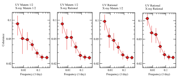
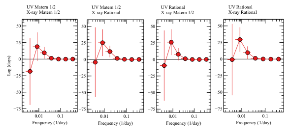
Figure 7: The coherence and lag spectra for Mrk 335. They are calculated by using 1000 pairs of gp lightcurve samples fit to the observed lightcurves. The error bars are the standard errors of the corresponding measurements for the 1000 samples. Different panels are for different kernels. Positive lags imply that the X-ray band leads the UVW2 band.

In this section, we calculate the coherence between the UVW2 and X-ray emission from Mrk 335  in search of evidence of lag features in the Fourier frequency domain. The coherence and lag spectra are estimated from one thousand pairs of UVW2 and X-ray gp lightcurve samples drawn from the Gaussian process posterior for each kernel. The lags are defined as the phase lags divided by the corresponding Fourier frequency. A similar approach has been used in other disciplines (e.g. Fabian et al., 2009; Kara et al., 2013). We consider both Matern $\frac{1}{2}$ and Rational Quadratic kernels. The results are shown in Figure 7. Positive lags imply that the X-ray variability leads the UVW2 variability. The error bars in the figure are the standard errors of the corresponding measurements for the one thousand samples.

The coherence between the UVW2 and X-ray emission decreases with frequency, suggesting more coherent variability at lower frequency. Positive lag features are shown at the low frequencies in the range $f=$ 0.005–0.025 d^-1. The absolute value of the lag at $f=0.0039\pm 0.0014$ d^-1 is estimated to be $19\pm 22$ days for the Matern $\frac{1}{2}$ kernel applied to both lightcurves and $29\pm 19$ days for the rational quadratic kernel, however both measurements are consistent with zero lag in the $2\sigma$ uncertainty range.

Tentative evidence of a shorter time lag at a higher frequency of $f=0.018\pm 0.006$ d^-1 is also found. The longer lag feature at a lower frequency would correspond to a more extended emission region while the shorter lag feature at a higher frequency would correspond to a more compact region. This could be explained by the presence of an extended UV emission region on the disc where reverberation happens.

Given that the lags are consistent with zero lag within $2\sigma$ uncertainty ranges, we conclude that only tentative evidence for a broad lag feature is found by applying Gaussian processes to the UVW2 and X-ray lightcurves of Mrk 335. Previous attempts to identify lags between two wavelengths of Mrk 335 based on cross-correlation analysis in the time domain suggests similar results (e.g. Gallo et al., 2018).

6 Conclusions

Following the interpolation of the unevenly-sampled lightcurves of Mrk 335 using Gaussian processes, tentative evidence for broad lag features is found in the Fourier frequency domain. The magnitude of the lags is consistent with previous cross-correlation analyses. In addition, the broad lag features might suggest an extended emission region e.g. of the disc in Mrk 335  during the reverberation processes. If the corona is compact within 5 $R_{\rm g}$ in Mrk 335 (Wilkins et al., 2015), our data suggest a possibly wide range of UVW2 emission radii.

The structure functions computed from the gp-interpolated lightcurves are consistent with those derived from the observational data and furthermore, illicit potential insights into the properties of the latent lightcurves. In particular, we show through a simulation study that it is possible that dips in the X-ray structure function may be produced by sampling artefacts arising from gaps in the lightcurve. In contrast, the gp structure functions show no dips. While this is not proof that the dip in the observational X-ray structure function is due to a sampling artefact, it does allude to the possibility. The UVW2 gp structure functions do not exhibit strong dependence on the choice of kernel with both Matern $\frac{1}{2}$ and rational quadratic showing up a broken power law with breaks at 139 and 155 days respectively. The X-ray structure functions however do show up differences between kernels with the rational quadratic kernel predicting a power law and the Matern 1/2 kernel predicting a broken power law.

From the Gaussian process modelling perspective, the ability to carry out Bayesian model selection affords a quantitative means of comparing analytic kernels under the marginal likelihood. It may be possible to incorporate further flexibility into the fitting procedure by making use of more sophisticated methods of kernel design (Duvenaud, 2014) in order to allow the assessment of fits of sums and products of analytic kernels or by leveraging advances in transforming Gaussian process priors via Deep Gaussian processes (Damianou and Lawrence, 2013) or normalising flows (Maroñas et al., 2021). Such approaches could be validated using simulations studies. Additionally, modelling the cross-correlation using multioutput Gaussian processes (de Wolff et al., 2021) may be an interesting avenue for comparison against the approach taken here. Lastly, Bayesian spectral density estimation (Tobar, 2018) may afford further flexibility through nonparametric modelling of the power spectral density in addition to nonparametric modelling of the lightcurve in the time domain. These improvements in Bayesian modelling machinery may help to minimise model misspecification and as such, enable more robust inferences to be made about the functional forms of the latent lightcurves.

7 Acknowledgements

Jiachen Jiang acknowledges support from the Tsinghua Shui’Mu Scholar Program and the Tsinghua Astrophysics Outstanding Fellowship.

Appendix A Additional Graphical Tests for Identifying the Flux Distribution

In Figure 8 we show probability-probability (P-P) plots and empirical cumulative distributions functions (ECDFs) as graphical distribution tests for Gaussianity. It may be observed qualitatively that both X-ray band log count rates and UVW2 flux are well-modelled by a Gaussian distribution.

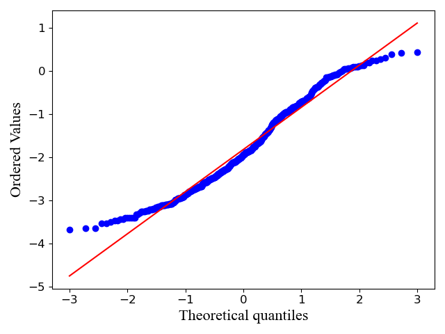
(a) PP plot for X-ray log count rates

(b) PP plot for UVW2 flux

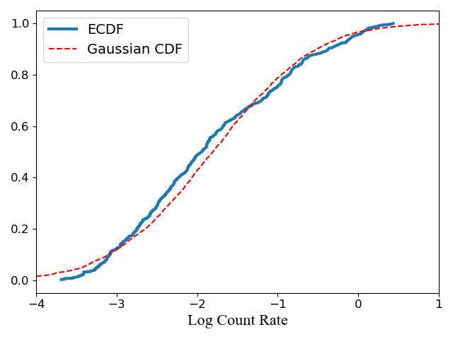
(c) ECDF for X-ray log count rates

(d) ECDF for UVW2 flux

Figure 8: P-P plots and ECDFs for X-ray log count rates and UVW2 flux. Graphical tests of Gaussianity. In the case of the P-P plots, proximity to the line is an indicator of Gaussianity. In the case of the ECDF plots, resemblance to the cumulative distribution function of a Gaussian is indicative of Gaussianity.

Appendix B Kernels

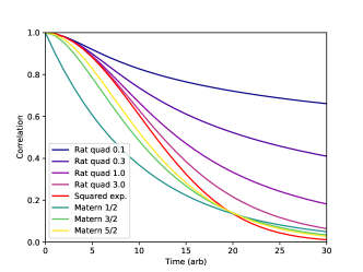
(a) Kernel autocorrelation functions

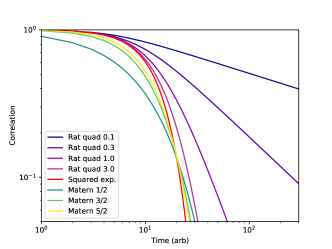
(b) Kernel log autocorrelation functions

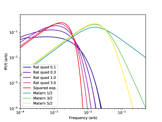
(c) Kernel PSDs

Figure 9: Kernel autocorrelation functions and PSDs. The rational quadratic kernel is plotted for different values of the $\alpha$ parameter. The Matern kernel plots in the PSD figure are offset by a factor of 10 for clarity. A PSD of $f^{-2}$ will match the high frequency part of the Matern $\frac{1}{2}$ kernel and the rational quadratic is endowed with additional flexibility to model PSDs by virtue of its $\alpha$ parameter. Such characteristics may explain why these kernels are preferred in the simulation study.

References

- (1)
- Aigrain et al. (2016) Aigrain, S., Parviainen, H. and Pope, B. (2016), ‘K2sc: flexible systematics correction and detrending of k2 light curves using gaussian process regression’, Monthly Notices of the Royal Astronomical Society 459(3), 2408–2419.
- Angus et al. (2018) Angus, R., Morton, T., Aigrain, S., Foreman-Mackey, D. and Rajpaul, V. (2018), ‘Inferring probabilistic stellar rotation periods using gaussian processes’, Monthly Notices of the Royal Astronomical Society 474(2), 2094–2108.
- Astropy Collaboration et al. (2018) Astropy Collaboration, Price-Whelan, A. M., Sipőcz, B. M., Günther, H. M., Lim, P. L., Crawford, S. M., Conseil, S., Shupe, D. L., Craig, M. W., Dencheva, N., Ginsburg, A., Vand erPlas, J. T., Bradley, L. D., Pérez-Suárez, D., de Val-Borro, M., Aldcroft, T. L., Cruz, K. L., Robitaille, T. P., Tollerud, E. J., Ardelean, C., Babej, T., Bach, Y. P., Bachetti, M., Bakanov, A. V., Bamford, S. P., Barentsen, G., Barmby, P., Baumbach, A., Berry, K. L., Biscani, F., Boquien, M., Bostroem, K. A., Bouma, L. G., Brammer, G. B., Bray, E. M., Breytenbach, H., Buddelmeijer, H., Burke, D. J., Calderone, G., Cano Rodríguez, J. L., Cara, M., Cardoso, J. V. M., Cheedella, S., Copin, Y., Corrales, L., Crichton, D., D’Avella, D., Deil, C., Depagne, É., Dietrich, J. P., Donath, A., Droettboom, M., Earl, N., Erben, T., Fabbro, S., Ferreira, L. A., Finethy, T., Fox, R. T., Garrison, L. H., Gibbons, S. L. J., Goldstein, D. A., Gommers, R., Greco, J. P., Greenfield, P., Groener, A. M., Grollier, F., Hagen, A., Hirst, P., Homeier, D., Horton, A. J., Hosseinzadeh, G., Hu, L., Hunkeler, J. S., Ivezić, Ž., Jain, A., Jenness, T., Kanarek, G., Kendrew, S., Kern, N. S., Kerzendorf, W. E., Khvalko, A., King, J., Kirkby, D., Kulkarni, A. M., Kumar, A., Lee, A., Lenz, D., Littlefair, S. P., Ma, Z., Macleod, D. M., Mastropietro, M., McCully, C., Montagnac, S., Morris, B. M., Mueller, M., Mumford, S. J., Muna, D., Murphy, N. A., Nelson, S., Nguyen, G. H., Ninan, J. P., Nöthe, M., Ogaz, S., Oh, S., Parejko, J. K., Parley, N., Pascual, S., Patil, R., Patil, A. A., Plunkett, A. L., Prochaska, J. X., Rastogi, T., Reddy Janga, V., Sabater, J., Sakurikar, P., Seifert, M., Sherbert, L. E., Sherwood-Taylor, H., Shih, A. Y., Sick, J., Silbiger, M. T., Singanamalla, S., Singer, L. P., Sladen, P. H., Sooley, K. A., Sornarajah, S., Streicher, O., Teuben, P., Thomas, S. W., Tremblay, G. R., Turner, J. E. H., Terrón, V., van Kerkwijk, M. H., de la Vega, A., Watkins, L. L., Weaver, B. A., Whitmore, J. B., Woillez, J., Zabalza, V. and Astropy Contributors (2018), ‘The Astropy Project: Building an Open-science Project and Status of the v2.0 Core Package’, AJ 156(3), 123.
- Astropy Collaboration et al. (2013) Astropy Collaboration, Robitaille, T. P., Tollerud, E. J., Greenfield, P., Droettboom, M., Bray, E., Aldcroft, T., Davis, M., Ginsburg, A., Price-Whelan, A. M., Kerzendorf, W. E., Conley, A., Crighton, N., Barbary, K., Muna, D., Ferguson, H., Grollier, F., Parikh, M. M., Nair, P. H., Unther, H. M., Deil, C., Woillez, J., Conseil, S., Kramer, R., Turner, J. E. H., Singer, L., Fox, R., Weaver, B. A., Zabalza, V., Edwards, Z. I., Azalee Bostroem, K., Burke, D. J., Casey, A. R., Crawford, S. M., Dencheva, N., Ely, J., Jenness, T., Labrie, K., Lim, P. L., Pierfederici, F., Pontzen, A., Ptak, A., Refsdal, B., Servillat, M. and Streicher, O. (2013), ‘Astropy: A community Python package for astronomy’, A&A 558, A33.
- Bartók et al. (2010) Bartók, A. P., Payne, M. C., Kondor, R. and Csányi, G. (2010), ‘Gaussian approximation potentials: The accuracy of quantum mechanics, without the electrons’, Physical review letters 104(13), 136403.
- Bond et al. (1998) Bond, J., Jaffe, A. H. and Knox, L. (1998), ‘Estimating the power spectrum of the cosmic microwave background’, Physical Review D 57(4), 2117.
- Buisson et al. (2017) Buisson, D. J. K., Lohfink, A. M., Alston, W. N. and Fabian, A. C. (2017), ‘Ultraviolet and X-ray variability of active galactic nuclei with Swift’, Monthly Notices of the Royal Astronomical Society 464(3), 3194–3218.
- Buisson et al. (2018) Buisson, D., Lohfink, A., Alston, W., Cackett, E., Chiang, C., Dauser, T., De Marco, B., Fabian, A., Gallo, L., Garcia, J. et al. (2018), ‘Is there a uv/x-ray connection in iras 13224- 3809?’, Monthly Notices of the Royal Astronomical Society 475(2), 2306–2313.
- Cai et al. (2020) Cai, Z.-Y., Wang, J.-X. and Sun, M. (2020), ‘EUCLIA. II. On the Puzzling Large UV to X-Ray Lags in Seyfert Galaxies’, The Astrophysical Journal 892(1), 63.
- Chartas et al. (2017) Chartas, G., Krawczynski, H., Zalesky, L., Kochanek, C. S., Dai, X., Morgan, C. W. and Mosquera, A. (2017), ‘Measuring the Innermost Stable Circular Orbits of Supermassive Black Holes’, The Astrophysical Journal 837(1), 26.
-
Cheng et al. (2020)
Cheng, B., Griffiths, R.-R., Wengert, S., Kunkel, C., Stenczel, T., Zhu, B.,
Deringer, V. L., Bernstein, N., Margraf, J. T., Reuter, K. and Csanyi, G. (2020), ‘Mapping materials and
molecules’, Accounts of Chemical Research 53(9), 1981–1991.
PMID: 32794697.
https://doi.org/10.1021/acs.accounts.0c00403 - Collier and Peterson (2001) Collier, S. and Peterson, B. M. (2001), ‘Characteristic ultraviolet/optical timescales in active galactic nuclei’, The Astrophysical Journal 555(2), 775.
- Covino et al. (2020) Covino, S., Landoni, M., Sandrinelli, A. and Treves, A. (2020), ‘Looking at blazar light-curve periodicities with gaussian processes’, The Astrophysical Journal 895(2), 122.
- Cowen-Rivers et al. (2021) Cowen-Rivers, A. I., Lyu, W., Tutunov, R., Wang, Z., Grosnit, A., Griffiths, R.-R., Jianye, H., Wang, J., Peters, J. and Bou-Ammar, H. (2021), ‘An Empirical Study of Assumptions in Bayesian Optimisation’, arXiv e-prints p. arXiv:2012.03826.
- Czekala et al. (2017) Czekala, I., Mandel, K. S., Andrews, S. M., Dittmann, J. A., Ghosh, S. K., Montet, B. T. and Newton, E. R. (2017), ‘Disentangling time-series spectra with gaussian processes: Applications to radial velocity analysis’, The Astrophysical Journal 840(1), 49.
- Damianou and Lawrence (2013) Damianou, A. and Lawrence, N. D. (2013), Deep Gaussian processes, in ‘Artificial Intelligence and Statistics’, PMLR, pp. 207–215.
- Davies and Harte (1987) Davies, R. B. and Harte, D. (1987), ‘Tests for hurst effect’, Biometrika 74(1), 95–101.
- de Wolff et al. (2021) de Wolff, T., Cuevas, A. and Tobar, F. (2021), ‘Mogptk: The multi-output Gaussian process toolkit’, Neurocomputing 424, 49–53.
- Deisenroth and Rasmussen (2011) Deisenroth, M. and Rasmussen, C. E. (2011), Pilco: A model-based and data-efficient approach to policy search, in ‘Proceedings of the 28th International Conference on machine learning (ICML-11)’, Citeseer, pp. 465–472.
- Dexter and Fragile (2011) Dexter, J. and Fragile, P. C. (2011), ‘Observational Signatures of Tilted Black Hole Accretion Disks from Simulations’, The Astrophysical Journal 730(1), 36.
- di Clemente et al. (1996) di Clemente, A., Giallongo, E., Natali, G., Trevese, D. and Vagnetti, F. (1996), ‘The variability of quasars. ii. frequency dependence’, The Astrophysical Journal 463, 466.
- Diamond-Lowe et al. (2020) Diamond-Lowe, H., Berta-Thompson, Z., Charbonneau, D., Dittmann, J. and Kempton, E. M.-R. (2020), ‘Simultaneous optical transmission spectroscopy of a terrestrial, habitable-zone exoplanet with two ground-based multiobject spectrographs’, The Astronomical Journal 160(1), 27.
- Durrande et al. (2016) Durrande, N., Hensman, J., Rattray, M. and Lawrence, N. D. (2016), ‘Detecting periodicities with gaussian processes’, PeerJ Computer Science 2, e50.
- Duvenaud (2014) Duvenaud, D. (2014), Automatic Model Construction with Gaussian Processes, PhD thesis, Computational and Biological Learning Laboratory, University of Cambridge.
- Edelson et al. (2000) Edelson, R., Koratkar, A., Nandra, K., Goad, M., Peterson, B. M., Collier, S., Krolik, J., Malkan, M., Maoz, D., O’Brien, P., Shull, J. M., Vaughan, S. and Warwick, R. (2000), ‘Intensive HST, RXTE, and ASCA Monitoring of NGC 3516: Evidence against Thermal Reprocessing’, The Astrophysical Journal 534(1), 180–188.
- Fabian et al. (2009) Fabian, A. C., Zoghbi, A., Ross, R. R., Uttley, P., Gallo, L. C., Brandt, W. N., Blustin, A. J., Boller, T., Caballero-Garcia, M. D., Larsson, J., Miller, J. M., Miniutti, G., Ponti, G., Reis, R. C., Reynolds, C. S., Tanaka, Y. and Young, A. J. (2009), ‘Broad line emission from iron K- and L-shell transitions in the active galaxy 1H0707-495’, Nature 459, 540–542.
- Gallo (2018) Gallo, L. (2018), X-ray perspective of Narrow-line Seyfert 1 galaxies, in ‘Revisiting Narrow-Line Seyfert 1 Galaxies and their Place in the Universe’, p. 34.
- Gallo et al. (2018) Gallo, L. C., Blue, D. M., Grupe, D., Komossa, S. and Wilkins, D. R. (2018), ‘Eleven years of monitoring the Seyfert 1 Mrk 335 with Swift: Characterizing the X-ray and UV/optical variability’, Monthly Notices of the Royal Astronomical Society 478(2), 2557–2568.
- Gallo et al. (2013) Gallo, L. C., Fabian, A. C., Grupe, D., Bonson, K., Komossa, S., Longinotti, A. L., Miniutti, G., Walton, D. J., Zoghbi, A. and Mathur, S. (2013), ‘A blurred reflection interpretation for the intermediate flux state in Mrk 335’, Monthly Notices of the Royal Astronomical Society 428(2), 1191–1200.
- Gallo et al. (2015) Gallo, L. C., Wilkins, D. R., Bonson, K., Chiang, C. Y., Grupe, D., Parker, M. L., Zoghbi, A., Fabian, A. C., Komossa, S. and Longinotti, A. L. (2015), ‘Suzaku observations of Mrk 335: confronting partial covering and relativistic reflection’, Monthly Notices of the Royal Astronomical Society 446(1), 633–650.
- Gardner and Done (2017) Gardner, E. and Done, C. (2017), ‘The origin of the UV/optical lags in NGC 5548’, Monthly Notices of the Royal Astronomical Society 470(3), 3591–3605.
- Gaskell and Klimek (2003) Gaskell, C. M. and Klimek, E. S. (2003), ‘Variability of Active Galactic Nuclei from Optical to X-ray Regions’, Astronomical and Astrophysical Transactions 22(4-5), 661–680.
- Gezari et al. (2013) Gezari, S., Martin, D. C., Forster, K., Neill, J. D., Huber, M., Heckman, T., Bianchi, L., Morrissey, P., Neff, S. G., Seibert, M., Schiminovich, D., Wyder, T. K., Burgett, W. S., Chambers, K. C., Kaiser, N., Magnier, E. A., Price, P. A. and Tonry, J. L. (2013), ‘The GALEX Time Domain Survey. I. Selection and Classification of Over a Thousand Ultraviolet Variable Sources’, The Astrophysical Journal 766(1), 60.
- Gibson et al. (2012) Gibson, N., Aigrain, S., Roberts, S., Evans, T., Osborne, M. and Pont, F. (2012), ‘A gaussian process framework for modelling instrumental systematics: application to transmission spectroscopy’, Monthly Notices of the Royal Astronomical Society 419(3), 2683–2694.
- Gordon et al. (2020) Gordon, T. A., Agol, E. and Foreman-Mackey, D. (2020), ‘A fast, two-dimensional gaussian process method based on celerite: Applications to transiting exoplanet discovery and characterization’, The Astronomical Journal 160(5), 240.
- Greeff and Schoellig (2020) Greeff, M. and Schoellig, A. P. (2020), ‘Exploiting differential flatness for robust learning-based tracking control using Gaussian processes’, IEEE Control Systems Letters 5(4), 1121–1126.
- Griffiths et al. (2019) Griffiths, R.-R., Aldrick, A. A., Garcia-Ortegon, M., Lalchand, V. R. and Lee, A. A. (2019), ‘Achieving Robustness to Aleatoric Uncertainty with Heteroscedastic Bayesian Optimisation’, arXiv e-prints p. arXiv:1910.07779.
- Griffiths and Hernández-Lobato (2020) Griffiths, R.-R. and Hernández-Lobato, J. M. (2020), ‘Constrained Bayesian optimization for automatic chemical design using variational autoencoders’, Chemical Science 11(2), 577–586.
- Grosnit et al. (2020) Grosnit, A., Cowen-Rivers, A. I., Tutunov, R., Griffiths, R.-R., Wang, J. and Bou-Ammar, H. (2020), ‘Are we Forgetting about Compositional Optimisers in Bayesian Optimisation?’, arXiv e-prints p. arXiv:2012.08240.
- Grosnit et al. (2021) Grosnit, A., Tutunov, R., Maraval, A. M., Griffiths, R.-R., Cowen-Rivers, A. I., Yang, L., Zhu, L., Lyu, W., Chen, Z., Wang, J., Peters, J. and Bou-Ammar, H. (2021), ‘High-Dimensional Bayesian Optimisation with Variational Autoencoders and Deep Metric Learning’, arXiv e-prints p. arXiv:2106.03609.
- Grupe et al. (2007) Grupe, D., Komossa, S. and Gallo, L. C. (2007), ‘Discovery of the Narrow-Line Seyfert 1 Galaxy Markarian 335 in a Historical Low X-Ray Flux State’, The Astrophysical Journal Letters 668(2), L111–L114.
- Grupe et al. (2012) Grupe, D., Komossa, S., Gallo, L. C., Longinotti, A. L., Fabian, A. C., Pradhan, A. K., Gruberbauer, M. and Xu, D. (2012), ‘A Remarkable Long-term Light Curve and Deep, Low-state Spectroscopy: Swift and XMM-Newton Monitoring of the NLS1 Galaxy Mkn 335’, The Astrophysical Journal Supplement Series 199(2), 28.
- Hase et al. (2020) Hase, F., Aldeghi, M., Hickman, R. J., Roch, L. M. and Aspuru-Guzik, A. (2020), ‘Gryffin: An algorithm for Bayesian optimization of categorical variables informed by expert knowledge’, arXiv e-prints p. arXiv:2003.12127.
- Hughes et al. (1992) Hughes, P., Aller, H. and Aller, M. (1992), ‘The university of michigan radio astronomy data base. i-structure function analysis and the relation between bl lacertae objects and quasi-stellar objects’, The Astrophysical Journal 396, 469–486.
- Jiang et al. (2021) Jiang, J., Cheng, H., Gallo, L. C., Ho, L. C., Buisson, D. J. K., Fabian, A. C., Harrison, F. A., Parker, M. L., Reynolds, C. S., Steiner, J. F., Tomsick, J. A., Walton, D. J. and Yuan, W. (2021), ‘The awakening beast in the Seyfert 1 Galaxy KUG 1141+371 - I’, Monthly Notices of the Royal Astronomical Society 501(1), 916–932.
- Jones et al. (2017) Jones, D. E., Stenning, D. C., Ford, E. B., Wolpert, R. L., Loredo, T. J., Gilbertson, C. and Dumusque, X. (2017), ‘Improving exoplanet detection power: Multivariate gaussian process models for stellar activity’, arXiv preprint arXiv:1711.01318 .
- Kammoun et al. (2021) Kammoun, E. S., Dovčiak, M., Papadakis, I. E., Caballero-García, M. D. and Karas, V. (2021), ‘UV/Optical Disk Thermal Reverberation in Active Galactic Nuclei: An In-depth Study with an Analytic Prescription for Time-lag Spectra’, The Astrophysical Journal 907(1), 20.
- Kara et al. (2013) Kara, E., Fabian, A. C., Cackett, E. M., Uttley, P., Wilkins, D. R. and Zoghbi, A. (2013), ‘Discovery of high-frequency iron K lags in Ark 564 and Mrk 335’, Monthly Notices of the Royal Astronomical Society 434, 1129–1137.
- Karamanavis (2017) Karamanavis, V. (2017), ‘Gaussian processes for blazar variability studies’, Galaxies 5(1), 19.
- Karamanavis (2015) Karamanavis, V. V. (2015), Zooming into -ray loud galactic nuclei: broadband emission and structure dynamics of the blazar PKS 1502+ 106 and the narrow-line Seyfert 1 1H 0323+ 342, PhD thesis, Universität zu Köln.
- Komossa et al. (2020) Komossa, S., Grupe, D., Gallo, L., Poulos, P., Blue, D., Kara, E., Kriss, G., Longinotti, A., Parker, M. and Wilkins, D. (2020), ‘Lifting the curtain: The seyfert galaxy mrk 335 emerges from deep low-state in a sequence of rapid flare events’, Astronomy & Astrophysics 643, L7.
-
Langellier et al. (2021)
Langellier, N., Milbourne, T. W., Phillips, D. F., Haywood, R. D., Saar, S. H.,
Mortier, A., Malavolta, L., Thompson, S., Cameron, A. C., Dumusque, X.
and et al. (2021), ‘Detection
limits of low-mass, long-period exoplanets using gaussian processes applied
to harps-n solar radial velocities’, The Astronomical Journal 161(6), 287.
http://dx.doi.org/10.3847/1538-3881/abf1e0 - Longinotti et al. (2019) Longinotti, A. L., Kriss, G., Krongold, Y., Arellano-Cordova, K. Z., Komossa, S., Gallo, L., Grupe, D., Mathur, S., Parker, M. L., Pradhan, A. and Wilkins, D. (2019), ‘The XMM-Newton/HST View of the Obscuring Outflow in the Seyfert Galaxy Mrk 335 Observed at Extremely Low X-Ray Flux’, The Astrophysical Journal 875(2), 150.
- Longinotti et al. (2013) Longinotti, A. L., Krongold, Y., Kriss, G. A., Ely, J., Gallo, L., Grupe, D., Komossa, S., Mathur, S. and Pradhan, A. (2013), ‘The Rise of an Ionized Wind in the Narrow-line Seyfert 1 Galaxy Mrk 335 Observed by XMM-Newton and HST’, The Astrophysical Journal 766(2), 104.
- Luger, Foreman-Mackey and Hedges (2021a) Luger, R., Foreman-Mackey, D. and Hedges, C. (2021a), ‘Mapping stellar surfaces II: An interpretable Gaussian process model for light curves’, arXiv e-prints p. arXiv:2102.01697.
- Luger, Foreman-Mackey and Hedges (2021b) Luger, R., Foreman-Mackey, D. and Hedges, C. (2021b), ‘starry_process: Interpretable Gaussian processes for stellar light curves’, arXiv e-prints p. arXiv:2102.01774.
- Luger, Foreman-Mackey, Hedges and Hogg (2021) Luger, R., Foreman-Mackey, D., Hedges, C. and Hogg, D. W. (2021), ‘Mapping stellar surfaces I: Degeneracies in the rotational light curve problem’, arXiv e-prints p. arXiv:2102.00007.
- Lyon et al. (2020) Lyon, R., Hosenie, Z., Mootoovaloo, A., Stappers, B. and McBride, V. (2020), ‘Imbalance learning for variable star classification’, Monthly Notices of the Royal Astronomical Society 493(4), 6050–6059.
- MacKay (1992) MacKay, D. J. (1992), ‘Bayesian interpolation’, Neural Computation 4(3), 415–447.
- MacKay (1991) MacKay, D. J. C. (1991), Bayesian Methods for Adaptive Models, PhD thesis, California Institute of Technology.
- Maroñas et al. (2021) Maroñas, J., Hamelijnck, O., Knoblauch, J. and Damoulas, T. (2021), Transforming Gaussian processes with normalizing flows, in ‘International Conference on Artificial Intelligence and Statistics’, PMLR, pp. 1081–1089.
-
Matthews et al. (2017)
Matthews, A. G. d. G., van der Wilk, M., Nickson, T., Fujii, K.,
Boukouvalas, A., León-Villagrá, P., Ghahramani, Z. and Hensman, J. (2017), ‘GPflow: A
Gaussian process library using TensorFlow’, Journal of Machine
Learning Research 18(40), 1–6.
http://jmlr.org/papers/v18/16-537.html - McHardy et al. (2016) McHardy, I. M., Connolly, S. D., Peterson, B. M., Bieryla, A., Chand, H., Elvis, M. S., Emmanoulopoulos, D., Falco, E., Gandhi, P., Kaspi, S., Latham, D., Lira, P., McCully, C., Netzer, H. and Uemura, M. (2016), ‘The origin of UV-optical variability in AGN and test of disc models: XMM-Newton and ground-based observations of NGC 4395’, Astronomische Nachrichten 337(4-5), 500.
- Mchardy et al. (2004) Mchardy, I., Papadakis, I., Uttley, P., Page, M. J. and Mason, K. (2004), ‘Combined long and short time-scale x-ray variability of ngc 4051 with rxte and xmm-newton’, Monthly Notices of the Royal Astronomical Society 348, 783–801.
- Miller et al. (2010) Miller, L., Turner, T., Reeves, J., Lobban, A., Kraemer, S. and Crenshaw, D. (2010), ‘Spectral variability and reverberation time delays in the suzaku x-ray spectrum of ngc 4051’, Monthly Notices of the Royal Astronomical Society 403(1), 196–210.
- Morgan et al. (2008) Morgan, C. W., Kochanek, C. S., Dai, X., Morgan, N. D. and Falco, E. E. (2008), ‘X-Ray and Optical Microlensing in the Lensed Quasar PG 1115+080’, The Astrophysical Journal 689(2), 755–761.
- Moss and Griffiths (2020) Moss, H. B. and Griffiths, R.-R. (2020), ‘Gaussian Process Molecule Property Prediction with FlowMO’, arXiv e-prints p. arXiv:2010.01118.
- Moss et al. (2020) Moss, H., Leslie, D., Beck, D., Gonzalez, J. and Rayson, P. (2020), ‘Boss: Bayesian optimization over string spaces’, Advances in Neural Information Processing Systems 33.
- Murray (2008) Murray, I. (2008), ‘Introduction to Gaussian processes’.
- Mushotzky et al. (1993) Mushotzky, R. F., Done, C. and Pounds, K. A. (1993), ‘X-ray spectra and time variability of active galactic nuclei.’, Annual Review of Astronomy and Astrophysics 31, 717–717.
- Nigam et al. (2021) Nigam, A., Pollice, R., Hurley, M. F. D., Hickman, R. J., Aldeghi, M., Yoshikawa, N., Chithrananda, S., Voelz, V. A. and Aspuru-Guzik, A. (2021), ‘Assigning Confidence to Molecular Property Prediction’, arXiv e-prints p. arXiv:2102.11439.
- Nikolov et al. (2018) Nikolov, N., Sing, D. K., Fortney, J. J., Goyal, J. M., Drummond, B., Evans, T. M., Gibson, N. P., De Mooij, E. J., Rustamkulov, Z., Wakeford, H. R. et al. (2018), ‘An absolute sodium abundance for a cloud-free ‘hot saturn’exoplanet’, Nature 557(7706), 526–529.
-
Parker et al. (2019)
Parker, M. L., Longinotti, A. L., Schartel, N., Grupe, D., Komossa, S., Kriss,
G., Fabian, A. C., Gallo, L., Harrison, F. A., Jiang, J. and et al.
(2019), ‘The nuclear environment of the nls1
mrk 335: Obscuration of the x-ray line emission by a variable outflow’, Monthly Notices of the Royal Astronomical Society 490(1), 683–697.
http://dx.doi.org/10.1093/mnras/stz2566 - Parker et al. (2014) Parker, M. L., Wilkins, D. R., Fabian, A. C., Grupe, D., Dauser, T., Matt, G., Harrison, F. A., Brenneman, L., Boggs, S. E., Christensen, F. E., Craig, W. W., Gallo, L. C., Hailey, C. J., Kara, E., Komossa, S., Marinucci, A., Miller, J. M., Risaliti, G., Stern, D., Walton, D. J. and Zhang, W. W. (2014), ‘The NuSTAR spectrum of Mrk 335: extreme relativistic effects within two gravitational radii of the event horizon?’, Monthly Notices of the Royal Astronomical Society 443(2), 1723–1732.
- Pass et al. (2019) Pass, E. K., Cowan, N. B., Cubillos, P. E. and Sklar, J. G. (2019), ‘Estimating dayside effective temperatures of hot jupiters and associated uncertainties through gaussian process regression’, Monthly Notices of the Royal Astronomical Society 489(1), 941–950.
- Press et al. (1992) Press, W. H., Rybicki, G. B. and Hewitt, J. N. (1992), ‘The time delay of gravitational lens 0957+ 561. i-methodology and analysis of optical photometric data. ii-analysis of radio data and combined optical-radio analysis’, The Astrophysical Journal 385, 404–420.
- Pringle (1981) Pringle, J. E. (1981), ‘Accretion discs in astrophysics’, Annual Review of Astronomy and Astrophysics 19, 137–162.
- Rajpaul et al. (2015) Rajpaul, V., Aigrain, S., Osborne, M. A., Reece, S. and Roberts, S. (2015), ‘A Gaussian process framework for modelling stellar activity signals in radial velocity data’, Monthly Notices of the Royal Astronomical Society 452(3), 2269–2291.
- Rasmussen and Ghahramani (2001) Rasmussen, C. E. and Ghahramani, Z. (2001), Occam’s razor, in ‘Advances in Neural Information Processing Systems’, pp. 294–300.
- Rasmussen and Williams (2006) Rasmussen, C. E. and Williams, C. K. I. (2006), Gaussian Processes for Machine Learning, MIT Press.
- Reynolds (2000) Reynolds, C. S. (2000), ‘On the lack of x-ray iron line reverberation in mcg–6-30-15: Implications for the black hole mass and accretion disk structure’, The Astrophysical Journal 533(2), 811.
- Roberts et al. (2013) Roberts, S., Osborne, M., Ebden, M., Reece, S., Gibson, N. and Aigrain, S. (2013), ‘Gaussian processes for time-series modelling’, Philosophical Transactions of the Royal Society A: Mathematical, Physical and Engineering Sciences 371(1984), 20110550.
- Sánchez-Sáez et al. (2018) Sánchez-Sáez, P., Lira, P., Mejía-Restrepo, J., Ho, L. C., Arévalo, P., Kim, M., Cartier, R. and Coppi, P. (2018), ‘The QUEST-La Silla AGN Variability Survey: Connection between AGN Variability and Black Hole Physical Properties’, The Astrophysical Journal 864(1), 87.
- Shahriari et al. (2015) Shahriari, B., Swersky, K., Wang, Z., Adams, R. P. and De Freitas, N. (2015), ‘Taking the human out of the loop: A review of Bayesian optimization’, Proceedings of the IEEE 104(1), 148–175.
- Shakura and Sunyaev (1973) Shakura, N. I. and Sunyaev, R. A. (1973), ‘Reprint of 1973A&A….24..337S. Black holes in binary systems. Observational appearance.’, Astronomy and Astrophysics 500, 33–51.
- Shappee et al. (2014) Shappee, B. J., Prieto, J. L., Grupe, D., Kochanek, C. S., Stanek, K. Z., De Rosa, G., Mathur, S., Zu, Y., Peterson, B. M., Pogge, R. W., Komossa, S., Im, M., Jencson, J., Holoien, T. W. S., Basu, U., Beacom, J. F., Szczygieł, D. M., Brimacombe, J., Adams, S., Campillay, A., Choi, C., Contreras, C., Dietrich, M., Dubberley, M., Elphick, M., Foale, S., Giustini, M., Gonzalez, C., Hawkins, E., Howell, D. A., Hsiao, E. Y., Koss, M., Leighly, K. M., Morrell, N., Mudd, D., Mullins, D., Nugent, J. M., Parrent, J., Phillips, M. M., Pojmanski, G., Rosing, W., Ross, R., Sand, D., Terndrup, D. M., Valenti, S., Walker, Z. and Yoon, Y. (2014), ‘The Man behind the Curtain: X-Rays Drive the UV through NIR Variability in the 2013 Active Galactic Nucleus Outburst in NGC 2617’, The Astrophysical Journal 788(1), 48.
- Shemmer et al. (2001) Shemmer, O., Romano, P., Bertram, R., Brinkmann, W., Collier, S., Crowley, K. A., Detsis, E., Filippenko, A. V., Gaskell, C. M., George, T. A., Gliozzi, M., Hiller, M. E., Jewell, T. L., Kaspi, S., Klimek, E. S., Lannon, M. H., Li, W., Martini, P., Mathur, S., Negoro, H., Netzer, H., Papadakis, I., Papamastorakis, I., Peterson, B. M., Peterson, B. W., Pogge, R. W., Pronik, V. I., Rumstay, K. S., Sergeev, S. G., Sergeeva, E. A., Stirpe, G. M., Taylor, C. J., Treffers, R. R., Turner, T. J., Uttley, P., Vestergaard, M., von Braun, K., Wagner, R. M. and Zheng, Z. (2001), ‘Multiwavelength Monitoring of the Narrow-Line Seyfert 1 Galaxy Arakelian 564. III. Optical Observations and the Optical-UV-X-Ray Connection’, The Astrophysical Journal 561(1), 162–170.
- Simonetti et al. (1985) Simonetti, J., Cordes, J. and Heeschen, D. (1985), ‘Flicker of extragalactic radio sources at two frequencies’, The Astrophysical Journal 296, 46–59.
- Smith et al. (2018) Smith, K. L., Mushotzky, R. F., Boyd, P. T., Malkan, M., Howell, S. B. and Gelino, D. M. (2018), ‘The Kepler Light Curves of AGN: A Detailed Analysis’, The Astrophysical Journal 857(2), 141.
- Smith and Vaughan (2007) Smith, R. and Vaughan, S. (2007), ‘X-ray and optical variability of Seyfert 1 galaxies as observed with XMM-Newton’, Monthly Notices of the Royal Astronomical Society 375(4), 1479–1487.
- Starkey et al. (2017) Starkey, D., Horne, K., Fausnaugh, M. M., Peterson, B. M., Bentz, M. C., Kochanek, C. S., Denney, K. D., Edelson, R., Goad, M. R., De Rosa, G., Anderson, M. D., Arévalo, P., Barth, A. J., Bazhaw, C., Borman, G. A., Boroson, T. A., Bottorff, M. C., Brandt, W. N., Breeveld, A. A., Cackett, E. M., Carini, M. T., Croxall, K. V., Crenshaw, D. M., Dalla Bontà, E., De Lorenzo-Cáceres, A., Dietrich, M., Efimova, N. V., Ely, J., Evans, P. A., Filippenko, A. V., Flatland, K., Gehrels, N., Geier, S., Gelbord, J. M., Gonzalez, L., Gorjian, V., Grier, C. J., Grupe, D., Hall, P. B., Hicks, S., Horenstein, D., Hutchison, T., Im, M., Jensen, J. J., Joner, M. D., Jones, J., Kaastra, J., Kaspi, S., Kelly, B. C., Kennea, J. A., Kim, S. C., Kim, M., Klimanov, S. A., Korista, K. T., Kriss, G. A., Lee, J. C., Leonard, D. C., Lira, P., MacInnis, F., Manne-Nicholas, E. R., Mathur, S., McHardy, I. M., Montouri, C., Musso, R., Nazarov, S. V., Norris, R. P., Nousek, J. A., Okhmat, D. N., Pancoast, A., Parks, J. R., Pei, L., Pogge, R. W., Pott, J. U., Rafter, S. E., Rix, H. W., Saylor, D. A., Schimoia, J. S., Schnülle, K., Sergeev, S. G., Siegel, M. H., Spencer, M., Sung, H. I., Teems, K. G., Turner, C. S., Uttley, P., Vestergaard, M., Villforth, C., Weiss, Y., Woo, J. H., Yan, H., Young, S., Zheng, W. and Zu, Y. (2017), ‘Space Telescope and Optical Reverberation Mapping Project.VI. Reverberating Disk Models for NGC 5548’, The Astrophysical Journal 835(1), 65.
- Stein (2012) Stein, M. L. (2012), Interpolation of spatial data: some theory for kriging, Springer Science & Business Media.
- Thawani et al. (2020) Thawani, A. R., Griffiths, R.-R., Jamasb, A., Bourached, A., Jones, P., McCorkindale, W., Aldrick, A. A. and Lee, A. A. (2020), ‘The Photoswitch Dataset: A Molecular Machine Learning Benchmark for the Advancement of Synthetic Chemistry’, arXiv e-prints p. arXiv:2008.03226.
- Timmer and König (1995) Timmer, J. and König, M. (1995), ‘On generating power law noise.’, Astronomy and Astrophysics 300, 707.
- Tobar (2018) Tobar, F. (2018), Bayesian nonparametric spectral estimation, in ‘Advances in Neural Information Processing Systems’, pp. 10127–10137.
- Tobar et al. (2015) Tobar, F., Bui, T. D. and Turner, R. E. (2015), Learning stationary time series using gaussian processes with nonparametric kernels, in ‘Advances in Neural Information Processing Systems’, pp. 3501–3509.
-
Tripathi et al. (2020)
Tripathi, S., McGrath, K. M., Gallo, L. C., Grupe, D., Komossa, S., Berton, M.,
Kriss, G. and Longinotti, A. L. (2020), ‘Tracking the year-to-year variation in the spectral
energy distribution of the narrow-line seyfert 1 galaxy mrk 335’, Monthly Notices of the Royal Astronomical Society 499(1), 1266–1286.
http://dx.doi.org/10.1093/mnras/staa2817 - Troyer et al. (2016) Troyer, J., Starkey, D., Cackett, E. M., Bentz, M. C., Goad, M. R., Horne, K. and Seals, J. E. (2016), ‘Correlated X-ray/ultraviolet/optical variability in NGC 6814’, Monthly Notices of the Royal Astronomical Society 456(4), 4040–4050.
- Uttley and McHardy (2005) Uttley, P. and McHardy, I. M. (2005), ‘X-ray variability of ngc 3227 and 5506 and the nature of active galactic nucleus ‘states”, Monthly Notices of the Royal Astronomical Society 363(2), 586–596.
- van der Wilk (2019) van der Wilk, M. (2019), Sparse Gaussian process approximations and applications, PhD thesis, University of Cambridge.
- Wang et al. (2012) Wang, Y., Khardon, R. and Protopapas, P. (2012), ‘Nonparametric bayesian estimation of periodic light curves’, The Astrophysical Journal 756(1), 67.
- Welsh et al. (2011) Welsh, B. Y., Wheatley, J. M. and Neil, J. D. (2011), ‘GALEX observations of quasar variability in the ultraviolet’, Astronomy and Astrophysics 527, A15.
-
Wilkins (2019)
Wilkins, D. R. (2019), ‘Low-frequency x-ray
timing with gaussian processes and reverberation in the radio-loud agn 3c
120’, Monthly Notices of the Royal Astronomical Society 489(2), 1957–1972.
http://dx.doi.org/10.1093/mnras/stz2269 - Wilkins et al. (2015) Wilkins, D. R., Gallo, L. C., Grupe, D., Bonson, K., Komossa, S. and Fabian, A. C. (2015), ‘Flaring from the supermassive black hole in Mrk 335 studied with Swift and NuSTAR’, Monthly Notices of the Royal Astronomical Society 454(4), 4440–4451.
- Xin et al. (2020) Xin, C., Charisi, M., Haiman, Z. and Schiminovich, D. (2020), ‘Correlation between optical and UV variability of a large sample of quasars’, Monthly Notices of the Royal Astronomical Society 495(1), 1403–1413.
-
Yang et al. (2021)
Yang, S., Yan, D., Zhang, P., Dai, B. and Zhang, L. (2021), ‘Gaussian process modeling fermi-lat -ray
blazar variability: A sample of blazars with -ray
quasi-periodicities’, The Astrophysical Journal 907(2), 105.
http://dx.doi.org/10.3847/1538-4357/abcbff - Yu and Richards (2021) Yu, W. and Richards, G. T. (2021), Accelerating CARMA modeling with Gaussian Processes, in ‘American Astronomical Society Meeting Abstracts’, Vol. 53 of American Astronomical Society Meeting Abstracts, p. 541.08.
- Zhang et al. (2020) Zhang, Y., Tang, Q., Zhang, Y., Wang, J., Stimming, U. and Lee, A. A. (2020), ‘Identifying degradation patterns of lithium ion batteries from impedance spectroscopy using machine learning’, Nature communications 11(1), 1–6.
- Zhu et al. (2016) Zhu, F.-F., Wang, J.-X., Cai, Z.-Y. and Sun, Y.-H. (2016), ‘The Timescale-dependent Color Variability of Quasars Viewed with /GALEX’, The Astrophysical Journal 832(1), 75.
- Zoghbi et al. (2013) Zoghbi, A., Reynolds, C. and Cackett, E. (2013), ‘Calculating time lags from unevenly sampled light curves’, The Astrophysical Journal 777(1), 24.