Accelerated differential inclusion for convex optimization

Abstract

This paper introduces a second-order differential inclusion for unconstrained convex optimization. In continuous level, solution existence in proper sense is obtained and exponential decay of a novel Lyapunov function along with the solution trajectory is derived as well. Then in discrete level, based on numerical discretizations of the continuous model, two inexact proximal point algorithms are proposed, and some new convergence rates are established via a discrete Lyapunov function.

Keywords: convex optimization; inexact proximal point algorithm; differential inclusion; existence; Lyapunov function; exponential decay; discretization; acceleration

1 Introduction

In this work, we investigate the accelerated differential inclusion

$$\gamma x^{\prime\prime}+(\mu+\gamma)x^{\prime}+\partial f(x)\ni\xi,$$ (1)

where $f:\mathcal{H}\to\,{\mathbb{R}}\cup\{+\infty\}$ is a proper and closed convex function on the finite-dimensional Hilbert space $\mathcal{H}$ and $\xi\in C([0,\infty);\mathcal{H})$ stands for small perturbation. The time scaling factor $\gamma$ in 1 is governed by $\gamma^{\prime}=\mu-\gamma$, and $\mu\geqslant 0$ stands for the strongly convex constant (cf. 7) of $f$. Throughout, $\mathcal{H}$ is equipped with the inner product $\left\langle{\cdot,\cdot}\right\rangle$ and the norm $\left\lVert{\cdot}\right\rVert=\sqrt{\left\langle{\cdot,\cdot}\right\rangle}$. Besides, assume ${\mathop{{\rm argmin}}\,}f\neq\emptyset$ and let $x^{*}\in{\mathop{{\rm argmin}}\,}f$ be a global minimizer of $f$.

Recently, many authors investigate first-order optimization methods from the ordinary differential equation point of view. The gradient flow [1] models the gradient descent method and the proximal point algorithm (PPA) [2]. The heavy ball system [3, 4] is associated with Polyak’s heavy ball method [5]. The asymptotic vanishing damping (AVD) model, which is derived in [6] and further studied and generalized in [7, 9], recoveries Nesterov accelerated gradient (NAG) method [10] and FISTA [11]. The dynamical systems considered in [12, 13, 14, 15, 16] are closely related to Nesterov’s optimal method [17, Chapter 2] based on estimate sequence technique. When $\xi=0$, the differential inclusion 1 reduces to the NAG flow proposed in our previous work [14].

Investigations of these dynamical systems with perturbation have also been studied by many authors. In [4, 18], the authors considered the following heavy ball system with perturbation

$$x^{\prime\prime}(t)+\alpha(t)x^{\prime}(t)+\nabla f(x(t))=\xi(t),\quad t>0,$$ (2)

where $\alpha(\cdot)$ is some continuous positive function on $\,{\mathbb{R}}_{+}$. However, only weak convergence result of the trajectory to 2 was established. The perturbed generalization of the AVD model [6] reads as follows

$$x^{\prime\prime}(t)+\frac{\alpha}{t^{\beta}}x^{\prime}(t)+\nabla f(x(t))=\xi(t),\quad t\geqslant t_{0}>0,$$ (3)

where $\alpha>0$ and $0\leqslant\beta\leqslant 1$. For $\beta=1$, under the assumption $\xi\in L^{1}_{\nu}(0,\infty;\mathcal{H})$ with $\nu(t)=(t+1)^{\min\{1,\alpha/3\}}$, the decay rate $O(t^{-\min\{3,2\alpha/3\}})$ can be found in [19, 7, 20]. Here and in the sequel, $L^{1}_{\nu}(0,\infty;\mathcal{H})$ denotes the standard $\mathcal{H}$-valued weighted $L^{1}$ space, with $\nu$ being some nonnegative measurable function on $(0,\infty)$. Balti and May [3] studied the case $0\leqslant\beta<1$ and established the rate $O(t^{-2\beta})$, provided that $\xi\in L^{1}_{\nu}(0,\infty;\mathcal{H})$ with $\nu(t)=(t+1)^{\beta}$. Those decay estimates yield the minimizing property of the solution trajectory $x(t)$, which converges weakly (or strongly under further assumption) to a limit in ${\mathop{{\rm argmin}}\,}f$. Based on this observation, Sebbouh et al. [21] analysed the convergence behaviour of 3 when $f$ satisfies some further local geometrical assumptions such as the flatness condition and the Łojasiewicz property, which are beyond the convexity of $f$. They proved that there exists $T\geqslant 0$ such that

$$f(x(t))-f(x^{*})+\left\lVert{x(t)-x^{*}}\right\rVert^{2}+\left\lVert{x^{\prime}(t)}\right\rVert^{2}\leqslant Ce^{-mt^{1-\beta}},\quad t\geqslant T,$$ (4)

with the condition $\xi\in L^{1}_{\nu}(0,\infty;\mathcal{H})$, where $\nu(t)=e^{mt^{1-\beta}}$, $m\in(0,2\theta/(2+\theta))$ with some $\theta\in[1,2]$ related to the local geometrical property of $f$. Particularly, if $f$ is strongly convex, then $\theta=1$ and $T=0$. Thus, 4 implies global exponential decay rate $O(e^{-2t/3})$, requiring that $\xi\in L^{1}_{\nu}(0,\infty;\mathcal{H})$ with $\nu(t)=e^{2t/3}$. However, for this case, our accelerated differential inclusion 1 can achieve the same decay rate under weaker assumption on $\xi$; see Theorem 2.3.

For the nonsmooth setting, it is worth noticing some works related to the corresponding differential inclusions. In this case, the gradient flow becomes a first-order differential inclusion [22]

$$x^{\prime}(t)+\partial f(x(t))\ni\xi(t),\quad t>0.$$ (5)

Since $\partial f$ is a set-valued maximal monotone operator, discontinuity can occur in $x^{\prime}$ and classical $C^{1}$ solution to 5 may not exist. For the second-order differential inclusion

$$x^{\prime\prime}(t)+\partial f(x(t))\ni\xi\big{(}t,x(t),x^{\prime}(t)\big{)},\quad t>0,$$ (6)

the concept of energy-conserving solution has been introduced by [23, 24]. Recently, Vassilis et al. [8] extended the AVD model [6] to the nonsmooth setting:

$$x^{\prime\prime}(t)+\frac{\alpha}{t}x^{\prime}(t)+\partial f(x(t))\ni 0,\quad\quad t\geqslant t_{0}>0,$$

which is a special case of 6. They obtained the existence of energy-conserving solution and established the minimizing property. Note that our model 1 can also be viewed as a particular case of 6, and therefore the existence of energy-conserving solution can be established. Moreover, we shall derive new exponential decay estimate

$$f(x(t))-f(x^{*})\leqslant e^{-t}\left(2\mathcal{L}_{0}+\left\lVert{\xi}\right\rVert^{2}_{L^{1}_{\nu}(0,t;\mathcal{H})}\right)\quad\text{ for all }t>0,$$

provided that $\xi\in L^{1}_{\nu}(0,\infty;\mathcal{H})$ with $\nu(t)=\sqrt{e^{t}/\gamma(t)}$. With weaker condition on $\xi$, e.g. $\left\lVert{\xi(t)}\right\rVert=O(t^{-p})$ with $p>0$, the rate $O(t^{-2p})$ can be obtained if $f$ is strongly convex assumption; see 2.2.

We now turn to algorithm aspect. Numerical discretizations for perturbed dynamical systems naturally lead to inexact optimization solvers such as inexact proximal gradient method (PGM), inexact PPA and the corresponding accelerated variants. On the other hand, convergence analyses of inexact convex optimization methods have already been widely studied. In summary, almost all the algorithms consider three types of approximations for the proximal mapping (see their definitions in Section 3.1).

In the pioneering work [2], Rockafellar has considered an inexact PPA using $type$-3 approximation, and the convergence result was derived with summable error. Then Güler [25] proposed an inexact accelerated PPA involving $type$-3 approximation as well and derived the rate $O(1/k^{2})$ with computation error $\varepsilon_{k}=O(1/k^{3/2})$. In [26], Salzo and Villa studied the convergence of an inexact PPA with $type$-1 approximation and proved the rate $O(1/k)$ with error $\varepsilon_{k}=O(1/k^{2})$. However, in Section 3, based on an implicit discretization of 1, we shall propose an inexact accelerated PPA using $type$-1 approximation and prove the improved rate $O(1/k^{2})$ with $\varepsilon_{k}=O(1/k^{2})$.

Villa et al. [27] extended the convergence result in [26] to an inexact accelerated PGM. Aujol and Dossal [28] investigated the inertial forward-backward algorithm with $type$-1 and $type$-2 approximations, and carefully studied the convergence rates under decay assumption on the error. Schmidt et al. [29] considered an accelerated PGM involving $type$-1 approximation and inexact gradient data. But no detailed convergence rate is given with specific error, saying $\varepsilon_{k}=O(1/k^{p})$. In Section 4, from a semi-implicit discretization of 1, we obtain an accelerated PGM which adopts $type$-1 approximation and inexact gradient data as well. We shall analyse both convex and strongly convex cases and present some new estimates. Particularly, for strongly convex case, we establish the rate $O(1/k^{2p})$ when the computation error decays like $O(1/k^{p})$.

To the end, we introduce some conventional functional spaces and list the arrangement of the rest part. Recall that $\left\lVert{\cdot}\right\rVert$ is the underlying norm of the Hilbert space $\mathcal{H}$; we also use $\left\lVert{\cdot}\right\rVert_{X}$ to denote the norm for any normed space $X$. Given $-\infty<a<b\leqslant\infty$, let $M(a,b;\mathcal{H})$ be the space of $\mathcal{H}$-valued Radon measures; for $k\in\mathbb{N}$, $C^{k}(a,b;\mathcal{H})$ stands for the space of $\mathcal{H}$-valued functions that are $k$-times continuous differentiable and set $C(a,b;\mathcal{H})=C^{0}(a,b;\mathcal{H})$; for $1\leqslant p\leqslant\infty$, $L^{p}(a,b;\mathcal{H})$ is the conventional $\mathcal{H}$-valued $L^{p}$ space and for $1\leqslant p<\infty$, denote by $L^{p}_{\nu}(a,b;\mathcal{H})$ the standard $\mathcal{H}$-valued weighted $L^{p}$ space, where $\nu$ is some nonnegative measurable function on $(a,b)$; for $k\in\mathbb{N}$, let $W^{k,\infty}(a,b;\mathcal{H})$ be an $\mathcal{H}$-valued Sobolev space [22]; the space of all $\mathcal{H}$-valued functions with bounded variation is defined by $BV(a,b;\mathcal{H})$ [22]. For $\mu\geqslant 0$, let $\mathcal{S}_{\mu}^{0}$ be the set of all properly closed convex functions on $\mathcal{H}$ such that

$$f(y)\geqslant f(x)+\left\langle{p,y-x}\right\rangle+\frac{\mu}{2}\left\lVert{x-y}\right\rVert^{2},$$ (7)

for all $x,y\in{\bf dom\,}f$ and $p\in\partial f(x)$. For $0\leqslant\mu\leqslant L<\infty$, we say $f\in\mathcal{S}_{\mu,L}^{1,1}$ if it belongs to $\mathcal{S}_{\mu}^{0}$ and has $L$-Lipschitz continuous gradient, i.e.,

$$\left\lVert{\nabla f(x)-\nabla f(y)}\right\rVert\leqslant L\left\lVert{x-y}\right\rVert\quad\text{ for all }x,y\in\mathcal{H}.$$

The rest of this paper is organized as follows. In Section 2, existence of the energy-conserving solution is established, and minimizing property of the solution trajectory is proved as well. Then in Sections 3 and 4, an inexact accelerated PPA and an inexact accelerated PGM are obtained, respectively, from the implicit and semi-implicit discretizations, and convergence rate estimates are derived by using the tool of discrete Lyapunov function. Finally, in Section 5, to investigate the performance of the proposed methods, two numerical experiments are presented.

2 Existence and Minimizing Property

In this section, assume $f\in\mathcal{S}_{\mu}^{0}$ with $\mu\geqslant 0$ and the interior of the domain of $f$, denoted by ${\rm int}\,{\bf dom\,}f$, is nonempty. We shall focus on the existence of energy-conserving solution (cf. 2.1) to the accelerated differential inclusion

$$\gamma x^{\prime\prime}+(\mu+\gamma)x^{\prime}+\partial f(x)\ni\xi,$$ (8)

with initial data

$$x(0)=x_{0}\in{\bf dom\,}f\quad\text{and}\quad x^{\prime}(0)=x_{1}\in\overline{\mathop{\cup}\limits_{\tau>0}\tau(x_{0}-\overline{{\bf dom\,}f})}.$$ (9)

The scaling factor $\gamma$ satisfies

$$\gamma^{\prime}=\mu-\gamma,\quad\gamma(0)=\gamma_{0}>0,$$ (10)

from which it is easy to obtain the exact solution $\gamma(t)=\mu+(\gamma_{0}-\mu)e^{-t}$. Hence $\gamma$ is positive and bounded, i.e., $\gamma_{\min}:=\min\{\gamma_{0},\mu\}\leqslant\gamma(t)\leqslant\max\{\gamma_{0},\mu\}=:\gamma_{\max}$ for all $t\geqslant 0$, and $\gamma(t)\to\mu$ as $t\to\infty$.

2.1 The Moreau–Yosida regularization

Given any $\lambda>0$, introduce the Moreau–Yosida regularization of $f$ by that [30]

$$f_{\lambda}(x):=\inf_{y\in\mathcal{H}}\left(f(y)+\frac{1}{2\lambda}\left\lVert{y-x}\right\rVert^{2}\right)\qquad\forall\,x\in\mathcal{H},$$ (11)

where the infimum is attained at the unique minimizer

$${\bf prox}_{\lambda f}(x):=\mathop{{\mathop{{\rm argmin}}\,}}\limits_{y\in\mathcal{H}}\left(f(y)+\frac{1}{2\lambda}\left\lVert{y-x}\right\rVert^{2}\right)\qquad\forall\,x\in\mathcal{H}.$$ (12)

Therefore, one must have

$$\frac{1}{\lambda}\left(x-{\bf prox}_{\lambda f}(x)\right)\in\partial f({\bf prox}_{\lambda f}(x)),$$ (13)

and it follows that any fixed-point of ${\bf prox}_{\lambda f}$ belongs to ${\mathop{{\rm argmin}}\,}f$. On the other hand, by definition, it is not hard to see (cf. [31, Remark 12.24])

$$f_{\lambda}(x)=f({\bf prox}_{\lambda f}(x))+\frac{1}{2\lambda}\left\lVert{x-{\bf prox}_{\lambda f}(x)}\right\rVert^{2},$$ (14)

and it holds $f({\bf prox}_{\lambda f}(x))\leqslant f_{\lambda}(x)\leqslant f(x)$ for all $x\in\mathcal{H}$. Hence, any $x^{*}\in{\mathop{{\rm argmin}}\,}f$ satisfies $x^{*}={\bf prox}_{\lambda f}(x^{*})$, and we conclude that $f_{\lambda}$ has the same minimizer and minimum as that of $f$. Besides, by [22, Proposition 17.2.2], we have the convergence property $\lim\limits_{\lambda\to 0}f_{\lambda}(x)=f(x)$ for all $x\in\mathcal{H}$.

By [22, Proposition 17.2.1], we have the identity $\nabla f_{\lambda}(x)=\frac{1}{\lambda}\left(x-{\bf prox}_{\lambda f}(x)\right)$, which, together with the firmly non-expansive property (see [31, Proposition 12.27])

$$(1+\lambda\mu)\left\lVert{{\bf prox}_{\lambda f}(x)-{\bf prox}_{\lambda f}(y)}\right\rVert^{2}\leqslant\left\langle{{\bf prox}_{\lambda f}(x)-{\bf prox}_{\lambda f}(y),x-y}\right\rangle,$$

implies that $(1+\lambda\mu)f_{\lambda}$ is $\mu$-strongly convex and $\nabla f_{\lambda}$ is $1/\lambda$-Lipschitz continuous for any fixed $\lambda>0$.

2.2 Energy-conserving solution

Following [23, 24], let us introduce the concept of energy-conserving solution.

Definition 2.1.

We call $x:[0,\infty)\to\mathcal{H}$ an energy-conserving solution to 8 with initial condition 9 if it satisfies the following.

• $x\in W^{1,\infty}_{loc}(0,\infty;\mathcal{H}),\,x(0)=x_{0}$ and $x(t)\in{\bf dom\,}f$ for all $t>0$.

• $x^{\prime}\in BV_{loc}([0,\infty);\mathcal{H}),\,x^{\prime}(0+)=x_{1}$.

• For almost all $t>0$, there holds the energy equality:

  $$f(x(t))+\frac{\gamma(t)}{2}\left\lVert{x^{\prime}(t)}\right\rVert^{2}+\int_{0}^{t}\frac{\mu+3\gamma(s)}{2}\left\lVert{x^{\prime}(s)}\right\rVert^{2}{\mathrm{d}}s$$

  $$={} f(x_{0})+\frac{\gamma_{0}}{2}\left\lVert{x_{1}}\right\rVert^{2}+\int_{0}^{t}\left\langle{\xi(s),x^{\prime}(s)}\right\rangle{\mathrm{d}}s.$$

• There exists some $\omega\in M(0,\infty;\mathcal{H})$ such that $\gamma x^{\prime\prime}+(\mu+\gamma)x^{\prime}+\omega=\xi$ holds in the sense of distributions, and for any $T>0$, we have

  $$\int_{0}^{T}\big{(}f(y(t))-f(x(t))\big{)}{\mathrm{d}}t\geqslant\left\langle{\omega,y-x}\right\rangle_{C([0,T];\mathcal{H})}\quad\text{for all }y\in C([0,T];\mathcal{H}).$$

Let $\lambda>0$ be given and set $F_{\lambda}=(1+\lambda\mu)f_{\lambda}$. According to Section 2.1, we know that $F_{\lambda}\in\mathcal{S}_{\mu,\mu+1/\lambda}^{1,1}$. Instead of 8, let us start from a family of regularized problem

$$\gamma x_{\lambda}^{\prime\prime}+(\mu+\gamma)x_{\lambda}^{\prime}+\nabla F_{\lambda}(x_{\lambda})=\xi,$$ (15)

with initial data $x_{\lambda}(0)=x_{0}$ and $x_{\lambda}^{\prime}(0)=x_{1}$. Since for any fixed $\lambda>0$, $\nabla F_{\lambda}$ is Lipschitz continuous, applying the standard Picard approximation argument (see the proof of [32, Theorem 7.3]) implies that 15 admits a unique solution $x_{\lambda}\in C^{2}([0,\infty);\mathcal{H})$.

In the following, we shall establish some priori estimates of $x_{\lambda}$, then take the limit $\lambda\to 0$ to obtain an energy-conserving solution to the original differential inclusion 8.

Lemma 2.1.

Let $\lambda>0$ be given such that $\lambda\mu\leqslant 1$. For any $T>0$, we have the estimate

$$\left\lVert{x^{\prime}_{\lambda}}\right\rVert_{C([0,T];\mathcal{H})}+\left\lVert{F_{\lambda}(x_{\lambda})}\right\rVert_{C([0,T])}+\left\lVert{x^{\prime\prime}_{\lambda}}\right\rVert_{L^{1}(0,T;\mathcal{H})}+\left\lVert{\nabla F_{\lambda}(x_{\lambda})}\right\rVert_{L^{1}(0,T;\mathcal{H})}\leqslant C_{1},$$ (16)

and moreover, if ${\bf dom\,}f=\mathcal{H}$, then

$$\left\lVert{x^{\prime\prime}_{\lambda}}\right\rVert_{C([0,T];\mathcal{H})}+\left\lVert{\nabla F_{\lambda}(x_{\lambda})}\right\rVert_{C([0,T];\mathcal{H})}\leqslant C_{2},$$ (17)

where both $C_{1}$ and $C_{2}$ are bounded and independent of $\lambda$.

Proof.

Following [23, Lemma 4.1], we can prove

$$\left\lVert{x^{\prime}_{\lambda}}\right\rVert_{C([0,T];\mathcal{H})}+\left\lVert{F_{\lambda}(x_{\lambda})}\right\rVert_{C([0,T])}\leqslant B_{1}<\infty,$$

and mimicking the proof of [23, Lemma 4.2], it is possible to establish

$$\left\lVert{x^{\prime\prime}_{\lambda}}\right\rVert_{L^{1}(0,T;\mathcal{H})}+\left\lVert{\nabla F_{\lambda}(x_{\lambda})}\right\rVert_{L^{1}(0,T;\mathcal{H})}\leqslant B_{2}<\infty.$$

Above, both $B_{1}$ and $B_{2}$ are independent of $\lambda$. Collecting them proves 16.

If ${\bf dom\,}f=\mathcal{H}$, then $f$ is continuous on $\mathcal{H}$ since it is convex. From 16, we conclude that $\left\lVert{x_{\lambda}}\right\rVert_{C([0,T];\mathcal{H})}\leqslant C_{3}$, where $C_{3}$ is independent of $\lambda$. Therefore, by [22, Proposition 9.5.2], $\partial f(x_{\lambda}(t))\neq\emptyset$ is a closed convex bounded set for all $t\in[0,T]$, and there exists some $C_{4}>0$, which is independent of $\lambda$ as well, such that

$$\sup_{0\leqslant t\leqslant T}\left\{\left\lVert{p}\right\rVert:\,p\in\partial f(x_{\lambda}(t))\right\}\leqslant C_{4}.$$

Hence, by [22, Proposition 17.2.2 (iii)], it follows that

$$\max_{0\leqslant t\leqslant T}\left\lVert{\nabla F_{\lambda}(x_{\lambda}(t))}\right\rVert=(1+\lambda\mu)\max_{0\leqslant t\leqslant T}\left\lVert{\nabla f_{\lambda}(x_{\lambda}(t))}\right\rVert\leqslant 2C_{4},$$

which together with 15 and 16 implies 17 and finishes the proof. ∎

Theorem 2.1.

The accelerated differential inclusion 8 admits an energy-conserving solution $x:[0,\infty)\to\mathcal{H}$ in the sense of 2.1, and if additionally ${\bf dom\,}f=\mathcal{H}$, then $x\in W^{2,\infty}_{loc}(0,\infty;\mathcal{H})\cap C^{1}([0,\infty);\mathcal{H})$ and 8 holds for almost all $t>0$.

Proof.

Given any $T>0$, according to the estimate 16, it is clear that $\{x_{\lambda}\}$ is equicontinuous and bounded in $C([0,T];\mathcal{H})$. Invoking the well-known Ascoli–Arzelà theorem (see [33, Theorem 6.4 on page 267]), there exists some $x\in C([0,T];\mathcal{H})$ and a subsequence which is also denoted by $\{x_{\lambda}\}$, such that $x_{\lambda}\overset{\lambda\to 0}{\longrightarrow}x$ in $C([0,T];\mathcal{H})$. As Lemma 2.1 also implies that $\{x^{\prime}_{\lambda}\}$ is bounded in $L^{\infty}(0,T;\mathcal{H})$, by [32, Corollary 3.30], there exists $z\in L^{\infty}(0,T;\mathcal{H})$ and a subsequence, such that

$$x^{\prime}_{\lambda}\overset{\lambda\to 0}{\longrightarrow}z \quad{\rm weak^{*}~{}in~{}}L^{\infty}(0,T;\mathcal{H}).$$ (18)

We conclude immediately that $z=x^{\prime}$ in the sense of distributions. This means $x\in W^{1,\infty}(0,T;\mathcal{H})$. Following [23, Lemmas 4.3, 4.4 and 4.5], one can verify that $x$ satisfies with all the rest conditions in 2.1, and moreover, for almost all $t\in(0,T)$,

$$F_{\lambda}(x_{\lambda}(t))\overset{\lambda\to 0}{\longrightarrow}f(x(t))\quad\text{and}\quad x^{\prime}_{\lambda}(t)\overset{\lambda\to 0}{\longrightarrow}x^{\prime}(t).$$ (19)

If ${\bf dom\,}f=\mathcal{H}$, then by Lemma 2.1, $\{x^{\prime}_{\lambda}\}$ is bounded and equicontinuous in $C([0,T];\mathcal{H})$. Invoking again the Ascoli–Arzelà theorem, there exits a subsequence (still denoted by $\{x^{\prime}_{\lambda}\}$), such that $x_{\lambda}^{\prime}$ converges to $x^{\prime}$ in $C([0,T];\mathcal{H})$. Moreover, we have $x^{\prime\prime}_{\lambda}\overset{\lambda\to 0}{\longrightarrow}v$ weak^∗ in $L^{\infty}(0,T;\mathcal{H})$, which indicates that $v$ is the generalized derivative of $x^{\prime}$. Therefore, $x\in W^{2,\infty}(0,T;\mathcal{H})\cap C^{1}([0,T];\mathcal{H})$ for any $T>0$. Analogously to 19, we have $F_{\lambda}(x_{\lambda})\overset{\lambda\to 0}{\longrightarrow}f(x)$ in $C([0,T])$. Now, invoking the proof technique proposed in [22, Theorem 17.2.2], one can establish

$$f(x)+f^{*}(\xi-\gamma x^{\prime\prime}-(\mu+\gamma)x^{\prime})=\left\langle{\xi-\gamma x^{\prime\prime}-(\mu+\gamma)x^{\prime},x}\right\rangle,$$

for almost all $t>0$, where $f^{*}$ denotes the conjugate function of $f$. By [22, Proposition 9.5.1], the above identity is equivalent to 8. This finishes the proof. ∎

2.3 Minimizing property

In this section, we shall prove the minimizing property of the energy-conserving solution to 8 and establish the decay rate by using Lyapunov functions.

Given any $\lambda>0$, let $x_{\lambda}$ be the unique solution to 15 and set $v_{\lambda}=x_{\lambda}+x_{\lambda}^{\prime}$, then we define $\mathcal{E}_{\lambda}(t):={}\mathcal{L}_{\lambda}(t)-\Xi_{\lambda}(t)$, where

$$\Xi_{\lambda}(t):={}\int_{0}^{t}e^{s-t}\left\langle{\xi(s),v_{\lambda}(s)-x^{*}}\right\rangle{\mathrm{d}}s,$$ (20)

$$\mathcal{L}_{\lambda}(t):={}F_{\lambda}(x_{\lambda}(t))-F_{\lambda}(x^{*})+\frac{\gamma(t)}{2}\left\lVert{v_{\lambda}(t)-x^{*}}\right\rVert^{2}.$$ (21)

We first establish the minimizing property of $x_{\lambda}$, then take the limit $\lambda\to 0$ to obtain the desired results.

Lemma 2.2.

Given any $\lambda>0$, it holds that

$$\mathcal{E}^{\prime}_{\lambda}(t)\leqslant-\mathcal{E}_{\lambda}(t)-\frac{\mu}{2}\left\lVert{x_{\lambda}^{\prime}(t)}\right\rVert^{2}\quad\text{ for all }0\leqslant t<\infty,$$ (22)

which implies

$$\mathcal{L}_{\lambda}(t)+\frac{\mu}{2}\int_{0}^{t}e^{s-t}\left\lVert{x_{\lambda}^{\prime}(s)}\right\rVert^{2}{\mathrm{d}}s\leqslant e^{-t}\left(2\mathcal{L}_{\lambda}(0)+R^{2}(t)\right),$$ (23)

where $R(t):=\int_{0}^{t}\left\lVert{\xi(s)}\right\rVert e^{s/2}/\sqrt{\gamma(s)}\,{\mathrm{d}}s$.

Proof.

According to [14, Lemma 3.2], it not hard to establish

$$\frac{\,{\rm d}}{\,{\rm d}t}\mathcal{L}_{\lambda}\leqslant-\mathcal{L}_{\lambda}-\frac{\mu}{2}\left\lVert{x_{\lambda}^{\prime}}\right\rVert^{2}+\left\langle{\xi,v_{\lambda}-x^{*}}\right\rangle,$$

and 22 follows immediately from this and the trivial identity $\Xi_{\lambda}^{\prime}=\left\langle{\xi,v_{\lambda}-x^{*}}\right\rangle-\Xi_{\lambda}$.

It remains to prove 23. By 22 we have

$$e^{t}\mathcal{E}_{\lambda}(t)+\frac{\mu}{2}\int_{0}^{t}e^{s}\left\lVert{x_{\lambda}^{\prime}(s)}\right\rVert^{2}{\mathrm{d}}s\leqslant\mathcal{E}_{\lambda}(0)=\mathcal{L}_{\lambda}(0),$$ (24)

which yields that

$$\frac{\gamma}{2}\left\lVert{v_{\lambda}-x^{*}}\right\rVert^{2}\leqslant\mathcal{L}_{\lambda}=\mathcal{E}_{\lambda}+\Xi_{\lambda}\leqslant{}\mathcal{L}_{\lambda}(0)e^{-t}+\int_{0}^{t}e^{s-t}\left\langle{\xi(s),v_{\lambda}(s)-x^{*}}\right\rangle{\mathrm{d}}s.$$

Thanks to Lemma A.1, we obtain

$$\sqrt{\gamma(t)}\left\lVert{v_{\lambda}(t)-x^{*}}\right\rVert\leqslant e^{-t/2}\left(\sqrt{2\mathcal{L}_{\lambda}(0)}+R(t)\right),$$

Based on this, $\Xi_{\lambda}$ can be estimated as follows

$$\Xi_{\lambda}(t)={} e^{-t}\int_{0}^{t}e^{s}\left\langle{\xi(s),v_{\lambda}(s)-x^{*}}\right\rangle{\mathrm{d}}s$$

$$\leqslant{} e^{-t}\int_{0}^{t}\frac{e^{s/2}}{\sqrt{\gamma(s)}}\left\lVert{\xi(s)}\right\rVert\cdot e^{s/2}\sqrt{\gamma(s)}\left\lVert{v_{\lambda}(s)-x^{*}}\right\rVert{\mathrm{d}}s$$

$$\leqslant{} e^{-t}\int_{0}^{t}\frac{e^{s/2}}{\sqrt{\gamma(s)}}\left\lVert{\xi(s)}\right\rVert\left(\sqrt{2\mathcal{L}_{\lambda}(0)}+R(s)\right){\mathrm{d}}s$$

$$={} e^{-t}\left(\sqrt{2\mathcal{L}_{\lambda}(0)}R(t)+\frac{1}{2}R^{2}(t)\right),$$

which together with 24 gives

$$\begin{split}\mathcal{L}_{\lambda}(t)+\frac{\mu}{2}\int_{0}^{t}e^{s-t}\left\lVert{x_{\lambda}^{\prime}(s)}\right\rVert^{2}{\mathrm{d}}s\leqslant{}&e^{-t}\left(\mathcal{L}_{\lambda}(0)+\sqrt{2\mathcal{L}_{\lambda}(0)}R(t)+\frac{1}{2}R^{2}(t)\right)\\ \leqslant{}&e^{-t}\left(2\mathcal{L}_{\lambda}(0)+R^{2}(t)\right).\end{split}$$

This proves 23 and completes the proof of this lemma. ∎

Theorem 2.2.

If $f\in\mathcal{S}_{0}^{0}$ and $\xi$ satisfies

$$e^{-t/2}\int_{0}^{t}e^{s}\left\lVert{\xi(s)}\right\rVert{\rm d}s\overset{t\to\infty}{\longrightarrow}0,$$ (25)

then the accelerated differential inclusion 8 admits an energy-conserving solution $x:[0,\infty)\to\mathcal{H}$ satisfying

$$f(x(t))-f(x^{*})\leqslant 2\mathcal{L}_{0}e^{-t}+\frac{e^{-t}}{\gamma_{0}}\left(\int_{0}^{t}e^{s}\left\lVert{\xi(s)}\right\rVert{\rm d}s\right)^{2},$$ (26)

for almost all $t>0$, where $\mathcal{L}_{0}:=f(x_{0})-f(x^{*})+\frac{\gamma_{0}}{2}\left\lVert{x_{0}+x_{1}-x^{*}}\right\rVert^{2}$.

Proof.

By Section 2.1, we have

$$F_{\lambda}(x_{0})-F_{\lambda}(x^{*})=(1+\lambda\mu)(f_{\lambda}(x_{0})-f_{\lambda}(x^{*}))\leqslant(1+\lambda\mu)(f(x_{0})-f(x^{*})),$$

and thus $\mathcal{L}_{\lambda}(0)\leqslant(1+\lambda\mu)\mathcal{L}_{0}$, which together with 23 implies

$$\mathcal{L}_{\lambda}(t)\leqslant e^{-t}\left(2(1+\lambda\mu)\mathcal{L}_{0}+\left(\int_{0}^{t}\frac{e^{s/2}}{\sqrt{\gamma(s)}}\left\lVert{\xi(s)}\right\rVert\,{\mathrm{d}}s\right)^{2}\right).$$ (27)

Since $\mu=0$, by 10, we have $\gamma(t)=\gamma_{0}e^{-t}$. By the fact 19, taking the limit $\lambda\to 0$ yields that

$$f(x(t))-f(x^{*})+\frac{\gamma(t)}{2}\left\lVert{x(t)+x^{\prime}(t)-x^{*}}\right\rVert^{2}\leqslant 2e^{-t}\mathcal{L}_{0}+\frac{e^{-t}}{\gamma_{0}}\left(\int_{0}^{t}e^{s}\left\lVert{\xi(s)}\right\rVert{\mathrm{d}}s\right)^{2},$$

for almost all $t>0$. This implies 26 and completes the proof of Theorem 2.2. ∎

Remark 2.1.

If $\xi\in L^{1}_{e^{t}}(0,\infty;\mathcal{H})$, then 25 is satisfied and from 26 we obtain the exponential decay

$$f(x(t))-f(x^{*})\leqslant e^{-t}\left(2\mathcal{L}_{0}+\frac{1}{\gamma_{0}}\left\lVert{\xi}\right\rVert^{2}_{L^{1}_{e^{t}}(0,\infty;\mathcal{H})}\right),\quad\text{ for almost all }t>0.$$

On the other hand, if $\xi(t)\leqslant e^{-t/2}(t+1)^{-p}$ with $p>0$, then by Lemma A.3,

$$\int_{0}^{t}e^{s}\left\lVert{\xi(s)}\right\rVert{\rm d}s\leqslant\int_{0}^{t}\frac{e^{s/2}}{(t+1)^{p}}{\rm d}s\leqslant\frac{C_{p}e^{t/2}}{(t+1)^{p}}.$$

Hence 25 is fulfilled and taking the above estimate into 26 yields

$$f(x(t))-f(x^{*})\leqslant 2\mathcal{L}_{0}e^{-t}+\frac{C_{p}/\gamma_{0}}{(t+1)^{2p}}.$$

Theorem 2.3.

If $f\in\mathcal{S}_{\mu}^{0}$ with $\mu>0$ and $\xi$ satisfies

$$e^{-t/2}\int_{0}^{t}e^{s/2}\left\lVert{\xi(s)}\right\rVert{\rm d}s\overset{t\to\infty}{\longrightarrow}0,$$ (28)

then the accelerated differential inclusion 8 admits an energy-conserving solution $x:[0,\infty)\to\mathcal{H}$ satisfying

$$f(x(t))-f(x^{*})+\frac{\gamma(t)}{2}\left\lVert{x(t)+x^{\prime}(t)-x^{*}}\right\rVert^{2}\leqslant 2\mathcal{L}_{0}e^{-t}+\frac{e^{-t}}{\gamma_{\min}}\left(\int_{0}^{t}e^{s/2}\left\lVert{\xi(s)}\right\rVert{\rm d}s\right)^{2},$$ (29)

for almost all $t>0$, where $\mathcal{L}_{0}=f(x_{0})-f(x^{*})+\frac{\gamma_{0}}{2}\left\lVert{x_{0}+x_{1}-x^{*}}\right\rVert^{2}$ and $\gamma_{\min}=\min\{\mu,\gamma_{0}\}>0$.

Proof.

As $\mu>0$, by the fact $\gamma(t)\geqslant\gamma_{\min}$ and Lemma A.3, we have

$$\int_{0}^{t}\frac{e^{s/2}}{\sqrt{\gamma(s)}}\left\lVert{\xi(s)}\right\rVert{\mathrm{d}}s\leqslant\frac{1}{\sqrt{\gamma_{\min}}}\int_{0}^{t}\frac{e^{s/2}}{(s+1)^{p}}\,{\mathrm{d}}s\leqslant{}\frac{C_{p}}{\sqrt{\gamma_{\min}}}\cdot\frac{e^{t/2}}{(t+1)^{p}},$$

and thus, by 19 and 27, taking the limit $\lambda\to 0$ gives

$$f(x(t))-f(x^{*})+\frac{\gamma(t)}{2}\left\lVert{x(t)+x^{\prime}(t)-x^{*}}\right\rVert^{2}\leqslant 2\mathcal{L}_{0}e^{-t}+\frac{C_{p}/\gamma_{\min}}{(t+1)^{2p}},$$

for almost all $t>0$, which proves 29 and concludes the proof of Theorem 2.3. ∎

Remark 2.2.

If $\xi\in L^{1}_{e^{t/2}}(0,\infty;\mathcal{H})$, then 28 holds true and by 29 we have the exponential decay

$$f(x(t))-f(x^{*})+\frac{\gamma(t)}{2}\left\lVert{x(t)+x^{\prime}(t)-x^{*}}\right\rVert^{2}\leqslant e^{-t}\left(2\mathcal{L}_{0}+\frac{1}{\gamma_{\min}}\left\lVert{\xi}\right\rVert^{2}_{L^{1}_{e^{t/2}}(0,\infty;\mathcal{H})}\right),$$

for almost all $t>0$. Besides, if $\xi(t)\leqslant(t+1)^{-p}$ with $p>0$, then invoking Lemma A.3 gives

$$\int_{0}^{t}e^{s/2}\left\lVert{\xi(s)}\right\rVert{\rm d}s\leqslant\int_{0}^{t}\frac{e^{s/2}}{(t+1)^{p}}{\rm d}s\leqslant\frac{C_{p}e^{t/2}}{(t+1)^{p}}.$$

This promises 28 and by 29 we find that

$$f(x(t))-f(x^{*})+\frac{\gamma(t)}{2}\left\lVert{x(t)+x^{\prime}(t)-x^{*}}\right\rVert^{2}\leqslant 2\mathcal{L}_{0}e^{-t}+\frac{C_{p}/\gamma_{\min}}{(t+1)^{2p}}.$$ (30)

3 An Inexact Accelerated PPA

In this section, we are mainly interested in the case $f\in\mathcal{S}_{\mu}^{0}$ with $\mu\geqslant 0$. Rewrite 8 as a first-order differential inclusion system

$${~{}\,}x^{\prime}=v-x,$$ (31a)

$$\gamma v^{\prime}\in\mu(x-v)-\partial f(x)+\xi,$$ (31b)

and consider the implicit Euler scheme

$$\frac{x_{k+1}-x_{k}}{\alpha_{k}}=v_{k+1}-x_{k+1},$$ (32a)

$$\gamma_{k}\frac{v_{k+1}-v_{k}}{\alpha_{k}}\in\mu(x_{k+1}-v_{k+1})-\partial f(x_{k+1})+\xi_{k},$$ (32b)

where the equation 10 of the scaling factor $\gamma$ is also discretized implicitly

$$\frac{\gamma_{k+1}-\gamma_{k}}{\alpha_{k}}=\mu-\gamma_{k+1},\quad\gamma_{0}>0.$$ (33)

After some manipulations, we rewrite 32a as follows

$$x_{k+1}={\bf prox}_{\lambda_{k}f}(w_{k}+\lambda_{k}\xi_{k}),\,\,\lambda_{k}={}\alpha_{k}^{2}/\eta_{k},$$ (34a)

$$v_{k+1}=x_{k+1}+\frac{x_{k+1}-x_{k}}{\alpha_{k}},$$ (34b)

where

$$w_{k}={}\frac{1}{\eta_{k}}(\gamma_{k}\alpha_{k}v_{k}+(\gamma_{k}+\mu\alpha_{k})x_{k}),\quad\eta_{k}=\gamma_{k}\alpha_{k}+\gamma_{k}+\mu\alpha_{k}.$$ (35)

Note that 34a gives a PPA with extrapolation. The additional term $\lambda_{k}\xi_{k}$ makes the proximal step (34a) inexact and it is more general to consider

$$x_{k+1}\approx{\bf prox}_{\lambda_{k}f}(w_{k}),$$ (36a)

$$v_{k+1}=x_{k+1}+\frac{x_{k+1}-x_{k}}{\alpha_{k}}.$$ (36b)

In the state of the art, we have many choices for (36a); see the inexact accelerated proximal point algorithms proposed in [25, 26]. In the forthcoming section, we shall list some typical approximations to the proximal mapping ${\bf prox}_{\lambda f}$.

3.1 Inexact proximal mapping

In [26], Salzo and Villa summarized three types of approximations from [34, 35, 2]. The first two of them involve the concept of $\varepsilon$-$subdi\!f\!\!f\!erential$:

$$\partial f(x,\varepsilon):=\left\{p\in\mathcal{H}:f(y)\geqslant f(x)+\left\langle{p,x-y}\right\rangle-\varepsilon\quad\forall\,y\in\mathcal{H}\right\}.$$

By definition, it is clear that $0\in\partial f(x,\varepsilon)$ iff $f(x)\leqslant\varepsilon+\inf_{y\in\mathcal{H}}f(y)$.

Definition 3.1 ([34]).

Given $\varepsilon,\,\lambda>0$ and $x\in\mathcal{H}$, we call $w\in\mathcal{H}$ a $type$-1 approximation of ${\bf prox}_{\lambda f}(x)$ with $\varepsilon$-precision and write $w=_{1,\varepsilon}\!{\bf prox}_{\lambda f}(x)$, if and only if $0\in\partial\phi_{\lambda}(w,\varepsilon^{2}/(2\lambda))$, where $\phi_{\lambda}(\cdot)=f(\cdot)+\frac{1}{2\lambda}\left\lVert{\cdot-x}\right\rVert^{2}$. Equivalently, $w=_{1,\varepsilon}\!{\bf prox}_{\lambda f}(x)$ if and only if

$$f(w)+\frac{1}{2\lambda}\left\lVert{w-x}\right\rVert^{2}\leqslant\frac{\varepsilon^{2}}{2\lambda}+f_{\lambda}(x).$$

Definition 3.2 ([35]).

Given $\varepsilon,\,\lambda>0$ and $x\in\mathcal{H}$, we call $w\in\mathcal{H}$ a $type$-2 approximation of ${\bf prox}_{\lambda f}(x)$ with $\varepsilon$-precision and write $w=_{2,\varepsilon}\!{\bf prox}_{\lambda f}(x)$, if and only if

$$\frac{x-w}{\lambda}\in\partial f(w,\varepsilon^{2}/(2\lambda)).$$

Definition 3.3 ([2]).

Given $\varepsilon,\,\lambda>0$ and $x\in\mathcal{H}$, we call $w\in\mathcal{H}$ a $type$-3 approximation of ${\bf prox}_{\lambda f}(x)$ with $\varepsilon$-precision and write $w=_{3,\varepsilon}\!{\bf prox}_{\lambda f}(x)$, iff ${\rm dist}\left(0,\partial\phi_{\lambda}(w)\right)\leqslant\frac{\varepsilon}{\lambda}$, where ${\rm dist}\left(0,\partial\phi_{\lambda}(w)\right):=\inf\left\{\left\lVert{p}\right\rVert:p\in\partial\phi_{\lambda}(w)\right\}$.

For practical approximations, we refer to [36]. Some variant of $type$-2 approximation can be found in [37]. The following result, coming from [26, Proposition 1], compares those three kinds of approximations. For more implications under further assumption, e.g., boundness of ${\bf dom\,}f$, see [27, Proposition 2.4].

Proposition 3.1 ([26]).

The following implications are true:

1. $w=_{2,\varepsilon}\!{\bf prox}_{\lambda f}(x)\,\Longrightarrow\,w=_{1,\varepsilon}\!{\bf prox}_{\lambda f}(x)$;

2. $w=_{3,\varepsilon}\!{\bf prox}_{\lambda f}(x)\,\Longrightarrow\,w=_{1,\varepsilon}\!{\bf prox}_{\lambda f}(x)$;

3. $w=_{3,\varepsilon}\!{\bf prox}_{\lambda f}(x)\,\Longleftrightarrow\,\!w={\bf prox}_{\lambda f}(x+e)$ with some $e\in\mathcal{H}$ such that $\left\lVert{e}\right\rVert\leqslant\varepsilon$.

Therefore, both $type$-2 and $type$-3 approximations can be reduced to $type$-1 approximation and the scheme 34a, as well as the implicit Euler discretization 32a, considers $type$-3 approximation. However, with same magnitude error $\varepsilon$, the corresponding PPA using $type$-2 and $type$-3 approximations has faster convergence rate. In other words, the decay assumption on $\varepsilon$ of $type$-2 and $type$-3 approximations is weaker than that of $type$-1 approximation.

Indeed, for convex $f$, Güler [25] proposed an inexact accelerated PPA involving $type$-3 approximation: $x_{k+1}=_{3,\varepsilon_{k}}\!{\bf prox}_{\lambda_{k}f}(w_{k})$; see [25, Section 2]. The rate $O(1/k^{2}+k^{1-2p})$ has been established (cf. [25, Theorem 3.3]) with

$$\lambda_{k}=\lambda>0\quad\text{and}\quad\varepsilon_{k}=C(k+1)^{-p}.$$ (37)

Salzo and Villa [26] presented an inexact accelerated PPA using $type$-2 approximation: $x_{k+1}=_{2,\varepsilon_{k}}\!\!{\bf prox}_{\lambda_{k}f}(w_{k})$ and they obtained the rate $O(1/k^{2}+k^{1-2p})$ as well, under assumption 37. Besides, they considered an inexact PPA that adopts $type$-1 approximation: $x_{k+1}=_{1,\varepsilon_{k}}\!{\bf prox}_{\lambda_{k}f}(w_{k})$. However, with the same condition 37, they only proved the rate $O(1/k+k^{3-2p})$ (see [26, Theorem 4]).

In the next section, we shall apply $type$-1 approximation to our inexact accelerated PPA 36a. Under assumption 37, for convex case ($\mu=0$), we derive the convergence rate $O(1/k^{2}+k^{2-2p})$ (cf. Theorem 3.1) which improves the result in [26, Theorem 4], and for strongly convex case ($\mu>0$), we take constant step size $\alpha_{k}=\alpha>0$ and obtain new convergence rate estimate (cf. Theorem 3.2).

To the end, we list a key lemma, which is important for our convergence rate analysis; see [38, Lemma 2.7] for a detailed proof.

Lemma 3.1 ([38]).

Assume $f\in\mathcal{S}_{\mu}^{0}$ with $\mu\geqslant 0$ and let $\varepsilon,\,\lambda>0$ and $x\in\mathcal{H}$ be given. Then for $w=_{1,\varepsilon}\!{\bf prox}_{\lambda f}(x)$, it holds that

$$\begin{split}\frac{\varepsilon^{2}}{2\lambda}+f(y)\geqslant{}&f(w)+\frac{1}{\lambda}\left\langle{\sigma+w-x,w-y}\right\rangle+\frac{\mu}{2}\left\lVert{w-y}\right\rVert^{2}+\frac{1+\lambda\mu}{2\lambda}\left\lVert{w-{\bf prox}_{\lambda f}(x)}\right\rVert^{2},\end{split}$$

for all $y\in\mathcal{H}$, where $\sigma=(1+\lambda\mu)({\bf prox}_{\lambda f}(x)-w)$. Particularly, taking $y=w$ gives

$$\left\lVert{w-{\bf prox}_{\lambda f}(x)}\right\rVert\leqslant\frac{\varepsilon}{\sqrt{1+\lambda\mu}}.$$

3.2 Main results and proofs

Given a nonnegative sequence $\{\varepsilon_{k}\}_{k=0}^{\infty}$, let us consider the scheme 36a with $type$-1 approximation:

$$x_{k+1}=_{1,\varepsilon_{k}}\!{\bf prox}_{\lambda_{k}f}(w_{k}),\,\,\lambda_{k}={}\alpha_{k}^{2}/\eta_{k},$$ (38a)

$$v_{k+1}=x_{k+1}+\frac{x_{k+1}-x_{k}}{\alpha_{k}},$$ (38b)

with $\eta_{k}$ and $w_{k}$ being defined by 35. Recall that the equation 10 of the scaling factor $\gamma$ is discretized implicitly by 33. It is worth noticing that 38a implies the identity

$$\frac{v_{k+1}-v_{k}}{\alpha_{k}}={}\frac{\mu}{\gamma_{k}}(x_{k+1}-v_{k+1})-\frac{1}{\gamma_{k}}\frac{w_{k}-x_{k+1}}{\lambda_{k}}.$$ (39)

To verify this, let $(\widehat{x}_{k+1},\widehat{v}_{k+1})$ satisfy

$$\left\{\begin{aligned} \frac{\widehat{x}_{k+1}-x_{k}}{\alpha_{k}}={}&\widehat{v}_{k+1}-\widehat{x}_{k+1},\\ \gamma_{k}\frac{\widehat{v}_{k+1}-v_{k}}{\alpha_{k}}\in{}&\mu(\widehat{x}_{k+1}-\widehat{v}_{k+1})-\partial f(\widehat{x}_{k+1}),\end{aligned}\right.$$

then it is evident that $\widehat{x}_{k+1}={}{\bf prox}_{\lambda_{k}f}(w_{k})$, where $\lambda_{k}$ and $w_{k}$ are the same as that in 38b. Based on this and 13, a direct manipulation verifies 39.

Assume that

$$\varepsilon_{k}\leqslant\frac{1}{(k+1)^{p}},\quad p>0.$$ (40)

Our main estimates are listed below.

Theorem 3.1.

Suppose $f\in\mathcal{S}_{0}^{0}$, i.e., $\mu=0$. If (i) $\gamma_{0}=4$, (ii) $\varepsilon_{k}$ obeys 40 with $p>1$ and (iii) $\alpha_{k}^{2}=\gamma_{k}(1+\alpha_{k})$, then for the scheme 38a, we have $\lambda_{k}=1$ and

$$f(x_{k})-f(x^{*})\leqslant\frac{2\mathcal{L}_{0}}{(k+1)^{2}}+C_{p}\left\{\begin{aligned} &\frac{1+\ln^{2}(k+1)}{(k+1)^{2}},&&p=2,\\ &(k+1)^{-2}+(k+1)^{2-2p},&&p>1\text{ and }p\neq 2,\end{aligned}\right.$$ (41)

where $\mathcal{L}_{0}:=f(x_{0})-f(x^{*})+\frac{\gamma_{0}}{2}\left\lVert{v_{0}-x^{*}}\right\rVert^{2}$.

Remark 3.1.

In the setting of Theorem 3.1 (except 40), if $\{k\varepsilon_{k}\}_{k=1}^{\infty}$ is summable, then we have the rate $O(1/k^{2})$ without log factor $\ln k$, which is promised by 48.

Theorem 3.2.

Suppose $f\in\mathcal{S}_{\mu}^{0}$ with $\mu>0$. If (i) $\gamma_{0}=\mu$, (ii) $\varepsilon_{k}$ satisfies 40 and we choose $\alpha_{k}=\alpha>0$, then for the scheme 38a, we have $\lambda_{k}={}\alpha^{2}/(\mu+2\mu\alpha)$ and

$$f(x_{k})-f(x^{*})+\frac{\mu}{2}\left\lVert{v_{k}-x^{*}}\right\rVert^{2}\leqslant\frac{2\mathcal{L}_{0}}{(1+\alpha)^{k}}+\frac{C_{\alpha,p,\mu}}{(k+1)^{2p}},$$ (42)

where $\mathcal{L}_{0}:=f(x_{0})-f(x^{*})+\frac{\gamma_{0}}{2}\left\lVert{v_{0}-x^{*}}\right\rVert^{2}$.

Remark 3.2.

Note that the estimate 42 matches the continuous decay rate 30. In addition, under the assumption of Theorem 3.2 (except 40), if we impose stronger condition that $\{(1+\alpha)^{k/2}\varepsilon_{k}\}_{k=0}^{\infty}$ is summable, then by 51 and 3.2, we have linear convergence rate $O((1+\alpha)^{-k})$.

To prove the above two theorems, we need several preparations. Let $\{(\gamma_{k},x_{k},v_{k})\}_{k=0}^{\infty}$ be generated by 33 and 38a. Define a discrete Lyapunov function

$$\mathcal{L}_{k}:=f(x_{k})-f(x^{*})+\frac{\gamma_{k}}{2}\left\lVert{v_{k}-x^{*}}\right\rVert^{2}\quad\text{ for all }k\in\mathbb{N},$$ (43)

and we also need two error accumulation functions

$$\left\{\begin{split}{}&\Upsilon_{0}={}0,\quad\Upsilon_{k}=\frac{1}{2}\sum_{i=0}^{k-1}\frac{\varepsilon_{i}^{2}}{\lambda_{i}\beta_{i+1}},\quad k\geqslant 1,\\ {}&\Omega_{0}={}0,\quad\Omega_{k}=\sum_{i=0}^{k-1}\frac{\alpha_{i}}{\lambda_{i}\beta_{i}}\cdot\sqrt{\frac{\beta_{i+1}}{\gamma_{i+1}}}\left\lVert{\xi_{i+1}}\right\rVert,\quad k\geqslant 1,\end{split}\right.$$

where $\xi_{k+1}=(1+\lambda_{k}\mu)({\bf prox}_{\lambda_{k}f}(w_{k})-x_{k+1})$ and

$$\beta_{0}={}1,\quad\beta_{k}=\prod_{i=0}^{k-1}\frac{1}{1+\alpha_{i}},\quad k\geqslant 1.$$ (44)

Lemma 3.2.

For the scheme 38a, we have

$$\mathcal{L}_{k}\leqslant 2\beta_{k}(\mathcal{L}_{0}+\Upsilon_{k}+\Omega^{2}_{k})\quad\text{ for all }k\in\mathbb{N}.$$ (45)

Proof.

Collecting 38b and 39, we see

$$\left\{\begin{split}\frac{x_{k+1}-x_{k}}{\alpha_{k}}={}&v_{k+1}-x_{k+1},\\ \frac{v_{k+1}-v_{k}}{\alpha_{k}}={}&\frac{\mu}{\gamma_{k}}(x_{k+1}-v_{k+1})-\frac{1}{\gamma_{k}}\frac{w_{k}-x_{k+1}}{\lambda_{k}}.\end{split}\right.$$

Thanks to this discretization formulation, we can follow the deduction from [14, Theorem 3.1] to obtain the difference

$$\begin{split}\mathcal{L}_{k+1}-\mathcal{L}_{k}={}&f(x_{k+1})-f(x_{k})-\frac{\alpha_{k}\gamma_{k+1}}{2}\left\lVert{v_{k+1}-x^{*}}\right\rVert^{2}-\frac{\gamma_{k}}{2}\left\lVert{v_{k+1}-v_{k}}\right\rVert^{2}\\ {}&\quad-\frac{1}{\lambda_{k}}\left\langle{w_{k}-x_{k+1},x_{k+1}-x_{k}}\right\rangle-\frac{\alpha_{k}}{\lambda_{k}}\left\langle{w_{k}-x_{k+1},x_{k+1}-x^{*}}\right\rangle\\ {}&\quad\qquad+\frac{\mu\alpha_{k}}{2}\left(\left\|x_{k+1}-x^{*}\right\|^{2}-\|x_{k+1}-v_{k+1}\|^{2}\right).\end{split}$$

Invoking Lemma 3.1, we have

$$\begin{split}-\frac{1}{\lambda_{k}}\left\langle{w_{k}-x_{k+1},x_{k+1}-x_{k}}\right\rangle\leqslant{}&\frac{\varepsilon_{k}^{2}}{2\lambda_{k}}+f(x_{k})-f(x_{k+1})-\frac{1}{\lambda_{k}}\left\langle{\xi_{k+1},x_{k+1}-x_{k}}\right\rangle,\end{split}$$

and

$$\begin{split}{}&-\frac{1}{\lambda_{k}}\left\langle{w_{k}-x_{k+1},x_{k+1}-x^{*}}\right\rangle\\ \leqslant{}&\frac{\varepsilon_{k}^{2}}{2\lambda_{k}}+f(x^{*})-f(x_{k+1})-\frac{1}{\lambda_{k}}\left\langle{\xi_{k+1},x_{k+1}-x^{*}}\right\rangle-\frac{\mu}{2}\left\lVert{x_{k+1}-x^{*}}\right\rVert^{2}.\end{split}$$

Consequently, it follows that

$$\begin{split}\mathcal{L}_{k+1}-\mathcal{L}_{k}\leqslant{}&-\alpha_{k}\mathcal{L}_{k+1}+\frac{1+\alpha_{k}}{2\lambda_{k}}\varepsilon_{k}^{2}-\frac{1}{\lambda_{k}}\left\langle{\xi_{k+1},x_{k+1}-x_{k}+\alpha_{k}(x_{k+1}-x^{*})}\right\rangle\\ {}&\quad-\frac{\mu\alpha_{k}}{2}\|x_{k+1}-v_{k+1}\|^{2}-\frac{\gamma_{k}}{2}\left\lVert{v_{k+1}-v_{k}}\right\rVert^{2}.\end{split}$$

Dropping surplus nonpositive terms and using 38b, we arrive at

$$\begin{split}\mathcal{L}_{k+1}-\mathcal{L}_{k}\leqslant{}&-\alpha_{k}\mathcal{L}_{k+1}+\frac{1+\alpha_{k}}{2\lambda_{k}}\varepsilon_{k}^{2}-\frac{\alpha_{k}}{\lambda_{k}}\left\langle{\xi_{k+1},v_{k+1}-x^{*}}\right\rangle\\ \leqslant{}&-\alpha_{k}\mathcal{L}_{k+1}+\frac{1+\alpha_{k}}{2\lambda_{k}}\varepsilon_{k}^{2}+\frac{\alpha_{k}}{\lambda_{k}}\left\lVert{\xi_{k+1}}\right\rVert\left\lVert{v_{k+1}-x^{*}}\right\rVert.\end{split}$$

Recursively, it holds that

$$\begin{split}\mathcal{L}_{k}\leqslant{}&\beta_{k}\mathcal{L}_{0}+\beta_{k}\sum_{i=0}^{k-1}\frac{1}{\beta_{i}}\left(\frac{1+\alpha_{i}}{2\lambda_{i}}\varepsilon_{i}^{2}+\frac{\alpha_{i}}{\lambda_{i}}\left\lVert{\xi_{i+1}}\right\rVert\left\lVert{v_{i+1}-x^{*}}\right\rVert\right)\\ ={}&\beta_{k}(\mathcal{L}_{0}+\Upsilon_{k})+\beta_{k}\sum_{i=0}^{k-1}\frac{\alpha_{i}}{\lambda_{i}\beta_{i}}\left\lVert{\xi_{i+1}}\right\rVert\left\lVert{v_{i+1}-x^{*}}\right\rVert.\end{split}$$ (46)

Note that above inequality implies

$$\frac{\gamma_{k}}{2}\left\lVert{v_{k}-x^{*}}\right\rVert^{2}\leqslant\beta_{k}\left(\mathcal{L}_{0}+\Upsilon_{k}\right)+\beta_{k}\sum_{i=0}^{k-1}\frac{\alpha_{i}}{\lambda_{i}\beta_{i}}\left\lVert{\xi_{i+1}}\right\rVert\left\lVert{v_{i+1}-x^{*}}\right\rVert.$$

Therefore, utilizing Lemma A.2 gives

$$\sqrt{\frac{\gamma_{k}}{\beta_{k}}}\left\lVert{v_{k}-x^{*}}\right\rVert\leqslant\sqrt{2(\mathcal{L}_{0}+\Upsilon_{k})}+2\sum_{i=0}^{k-1}\frac{\alpha_{i}\left\lVert{\xi_{i+1}}\right\rVert}{\lambda_{i}\beta_{i}}\sqrt{\frac{\beta_{i+1}}{\gamma_{i+1}}}=\sqrt{2(\mathcal{L}_{0}+\Upsilon_{k})}+2\Omega_{k}.$$

This can be reused for the estimate

$$\sum_{i=0}^{k-1}\frac{\alpha_{i}}{\lambda_{i}\beta_{i}}\left\lVert{\xi_{i+1}}\right\rVert\left\lVert{v_{i+1}-x^{*}}\right\rVert\leqslant{}\sum_{i=0}^{k-1}\frac{\alpha_{i}\left\lVert{\xi_{i+1}}\right\rVert}{\lambda_{i}\beta_{i}}\cdot\sqrt{\frac{\beta_{i+1}}{\gamma_{i+1}}}\cdot\left(\sqrt{2(\mathcal{L}_{0}+\Upsilon_{i})}+2\Omega_{i}\right)$$ (47)

$$={} \Omega_{k}^{2}+\sum_{i=0}^{k-1}\frac{\alpha_{i}\left\lVert{\xi_{i+1}}\right\rVert}{\lambda_{i}\beta_{i}}\cdot\sqrt{\frac{\beta_{i+1}}{\gamma_{i+1}}}\cdot\sqrt{2(\mathcal{L}_{0}+\Upsilon_{i})}\leqslant 2\Omega_{k}^{2}+\mathcal{L}_{0}+\Upsilon_{k}.$$

This together with 46 gives 45 and concludes the proof. ∎

We now arrive at a position for proving Theorems 3.1 and 3.2.

Proof of Theorem 3.1. By Lemma 3.1, we have $\left\lVert{\xi_{k+1}}\right\rVert\leqslant\varepsilon_{k}$. In view of 35 and our choice $\alpha_{k}^{2}=\gamma_{k}(1+\alpha_{k})$, it is easy to get $\lambda_{k}=1$. Observing 33, we conclude that $\beta_{k}=\gamma_{k}/\gamma_{0}$, and thus, it follows

$$\begin{split}\Upsilon_{k}={}&\frac{\gamma_{0}}{2}\sum_{i=0}^{k-1}\frac{\varepsilon_{i}^{2}}{\gamma_{i+1}},\quad\Omega_{k}={}\sqrt{\gamma_{0}}\sum_{i=0}^{k-1}\frac{\left\lVert{\xi_{i+1}}\right\rVert}{\sqrt{\gamma_{i+1}}}\leqslant\sqrt{\gamma_{0}}\sum_{i=0}^{k-1}\frac{\varepsilon_{i}}{\sqrt{\gamma_{i+1}}}.\end{split}$$

As Lemma A.4 implies

$$\frac{\gamma_{0}}{(\sqrt{\gamma_{0}}\,k+1)^{2}}\leqslant\gamma_{k}\leqslant\frac{4\gamma_{0}}{(\sqrt{\gamma_{0}}\,k+2)^{2}},$$

we obtain from Lemma 3.2 and the choice $\gamma_{0}=4$ that

$$\mathcal{L}_{k}\leqslant\frac{2\mathcal{L}_{0}}{(k+1)^{2}}+\frac{9}{(k+1)^{2}}\sum_{i=0}^{k-1}(i+1)^{2}\varepsilon_{i}^{2}+\frac{18}{(k+1)^{2}}\left(\sum_{i=0}^{k-1}(i+1)\varepsilon_{i}\right)^{2}.$$ (48)

Since $\varepsilon_{k}$ satisfies 40, invoking the following two elementary estimates:

$$\begin{split}{}&\sum_{i=0}^{k-1}(i+1)^{1-p}\leqslant 1+\int_{0}^{k}(s+1)^{1-p}\,{\rm d}s\leqslant{}\left\{\begin{aligned} &1+\ln(k+1),&&\text{ if }p=2,\\ &C_{p}\left(1+(k+1)^{2-p}\right),&&\text{ else},\end{aligned}\right.\end{split}$$ (49)

and

$$\begin{split}{}&\sum_{i=0}^{k-1}(i+1)^{2-2p}\leqslant 1+\int_{0}^{k}(s+1)^{2-2p}\,{\rm d}s\leqslant{}\left\{\begin{aligned} &1+\ln(k+1),&&\text{ if }p=3/2,\\ &C_{p}\left(1+(k+1)^{3-2p}\right),&&\text{ else},\end{aligned}\right.\end{split}$$ (50)

we finally establish 41 and finish the proof of Theorem 3.1. ∎

Proof of Theorem 3.2. Since $\gamma_{0}=\mu$, according to Lemma A.4, $\gamma_{k}=\mu$ and thus by 35, $\lambda_{k}=\lambda$. Moreover, by Lemma 3.1, $\left\lVert{\xi_{k+1}}\right\rVert\leqslant\varepsilon_{k}\sqrt{1+\lambda\mu}\leqslant\varepsilon_{k}\sqrt{1+\alpha}$. It follows immediately that

$$\Upsilon_{k}={}\frac{1}{2\lambda}\sum_{i=0}^{k-1}(1+\alpha)^{i+1}\varepsilon_{i}^{2},\quad\Omega_{k}\leqslant{}\frac{\sqrt{\alpha/\mu}}{\lambda}\sum_{i=0}^{k-1}(1+\alpha)^{(i+1)/2}\varepsilon_{i},$$ (51)

and we use 40 and 3.2 to get

$$\mathcal{L}_{k}\leqslant\frac{2\mathcal{L}_{0}}{(1+\alpha)^{k}}+\frac{C_{\alpha,p,\mu}}{(1+\alpha)^{k}}\left[\sum_{i=1}^{k}\frac{(1+\alpha)^{i}}{(i+1)^{2p}}+\left(\sum_{i=1}^{k}\frac{(1+\alpha)^{i/2}}{(i+1)^{p}}\right)^{2}\right].$$

Thus, applying A.1 proves 42 and concludes the proof of Theorem 3.2. ∎

4 An Inexact Accelerated PGM

We now move to the composite case $f=h+g$ where the smooth part $h\in\mathcal{S}_{\mu,L}^{1,1}$ with $0\leqslant\mu\leqslant L<\infty$ and the nonsmooth part $g\in\mathcal{S}_{0}^{0}$. In this case, the first-order system 31a becomes

$${~{}\,}x^{\prime}=v-x,$$ (52a)

$$\gamma v^{\prime}\in\mu(x-v)-\nabla h(x)-\partial g(x)+\xi.$$ (52b)

In the last section, we investigated an implicit scheme that involves the (approximated) gradient mapping ${\bf prox}_{\lambda_{k}f}$. However, for the current separable case $f=h+g$, it would be more efficient to use semi-implicit scheme, which means we use explicit scheme for smooth part $h$ and implicit scheme for nonsmooth part $g$. In other words, consider the splitting method

$$\frac{x_{k+1}-x_{k}}{\alpha_{k}}=v_{k+1}-x_{k+1},$$ (53a)

$$\gamma_{k}\frac{v_{k+1}-v_{k}}{\alpha_{k}}\in\mu(x_{k+1}-v_{k+1})-\nabla h(x_{k})-\partial g(x_{k+1})+\xi_{k},$$ (53b)

where the equation 10 of the scaling factor $\gamma$ is still discretized implicitly by 33.

4.1 Perturbed gradient mapping

Unlike the case (36a), the step (53b) involves inexact calculations of both $\nabla h(x_{k})$ and ${\bf prox}_{\lambda g}$. We can simply replace $\nabla h(x_{k})$ with inexact data $\widehat{\nabla}h(x_{k})$ [19, 39]. This really occurs if one applies Tikhonov regularization [40]. Approximations to ${\bf prox}_{\lambda g}$ mainly consider three types of inexact proximal mappings introduced in Section 3.1; see those methods in [37, 27].

Following [28, 29], we consider $type$-1 approximation to ${\bf prox}_{\lambda g}$ together with inexact data $\widehat{\nabla}h(x_{k})$. Note that in [28] only convex case is considered and that in [29, Propsitions 2 and 4], the convergence rates are established with accumulated errors (also see our Lemma 4.2) and no further decay rate is given with specific error, saying $\varepsilon_{k}=O(1/k^{p})$. We shall analyse both convex and strongly convex cases and present some new convergence rate estimates.

Motivated by [14, 41], for ease of analysis, we introduce the concept of perturbed gradient mapping. Given $\lambda>0,\,\tau\geqslant 0$ and $\varepsilon\geqslant 0$, define

$$\mathcal{G}_{\lambda f}(x,\tau,\varepsilon):={}\frac{1}{\lambda}(x-{S}_{\lambda f}(x,\tau,\varepsilon))\quad\text{ for all }x\in\mathcal{H},$$ (54)

where ${S}_{\lambda f}(x,\tau,\varepsilon)\approx_{1,\varepsilon}\!{\bf prox}_{\lambda g}(x-\lambda\widehat{\nabla}h(x))$ and $\widehat{\nabla}h(x)$ provides some approximation to $\nabla h(x)$ such that $\|\widehat{\nabla}h(x)-\nabla h(x)\|\leqslant\tau/\lambda$. For the case $\varepsilon=0$, we have ${S}_{\lambda f}(x,\tau,0)={\bf prox}_{\lambda g}(x-\lambda\widehat{\nabla}h(x))$ and by 13 we see that

$$\mathcal{G}_{\lambda f}(x,\tau,0)\in\widehat{\nabla}h(x)+\partial g\big{(}{S}_{\lambda f}(x,\tau,0)\big{)}.$$

Moreover, the following lemma is also crucial for our convergence analysis. Thanks to Lemma 3.1, the proof is the same as that of [14, Lemma 3] and we omit it here.

Lemma 4.1.

Let $\lambda>0,\,\tau\geqslant 0$ and $\varepsilon\geqslant 0$ be given. Assume $f=h+g$ where $h\in\mathcal{S}_{\mu,L}^{1,1}$ with $0\leqslant\mu\leqslant L<\infty$ and $g\in\mathcal{S}_{0}^{0}$. For any $x,y\in\mathcal{H}$, we have

$$\begin{split}\frac{\varepsilon^{2}}{2\lambda}+f(y)\geqslant{}&f\big{(}{S}_{\lambda f}(x,\tau,\varepsilon)\big{)}+\left\langle{\mathcal{G}_{\lambda f}(x,\tau,\varepsilon),y-x}\right\rangle+\frac{1}{\lambda}\left\langle{\sigma+e,y-S_{\lambda f}(x,\tau,\varepsilon)}\right\rangle\\ {}&\qquad+\frac{\mu}{2}\left\lVert{y-x}\right\rVert^{2}+\frac{\lambda}{2}(2-\lambda L)\left\lVert{\mathcal{G}_{\lambda f}(x,\tau,\varepsilon)}\right\rVert^{2},\end{split}$$

where $\sigma={S}_{\lambda f}(x,\tau,\varepsilon)-{S}_{\lambda f}(x,\tau,0)$ and $e=\lambda\big{(}\nabla h(x)-\widehat{\nabla}h(x)\big{)}$.

4.2 The proposed algorithm

Let $\{\varepsilon_{k}\}_{k=0}^{\infty}$ and $\{\tau_{k}\}_{k=0}^{\infty}$ be two nonnegative sequences. We make the step (53a) semi-implicit and plug the gradient mapping 54 into 53b to obtain

$$\frac{x_{k+1}-x_{k}}{\alpha_{k}}=v_{k}-x_{k+1},$$ (55a)

$$\frac{v_{k+1}-v_{k}}{\alpha_{k}}={}\frac{\mu}{\gamma_{k}}(x_{k+1}-v_{k+1})-\frac{1}{\gamma_{k}}\mathcal{G}_{\lambda_{k}f}(x_{k+1},\tau_{k},\varepsilon_{k}),$$ (55b)

where $\lambda_{k}>0$ and $\widehat{\nabla}h(x_{k})\approx\nabla h(x_{k})$ is some approximation such that $\|\widehat{\nabla}h(x_{k})-\nabla h(x_{k})\|\leqslant\tau_{k}/\lambda_{k}$.

Under the exact case $\tau_{k}=\varepsilon_{k}=0$, the scheme 55a has been considered in [14, Section 7.2], where, to promise the decay property of a Lyapunov function, an additional gradient descent step is supplemented. Hence, we also add an extra gradient step to 55a and obtain the following scheme:

$$\frac{y_{k}-x_{k}}{\alpha_{k}}={}v_{k}-y_{k},$$ (56a)

$$\frac{v_{k+1}-v_{k}}{\alpha_{k}}={}\frac{\mu}{\gamma_{k}}(y_{k}-v_{k+1})-\frac{1}{\gamma_{k}}\mathcal{G}_{\lambda_{k}f}(y_{k},\tau_{k},\varepsilon_{k}),$$ (56b)

$$x_{k+1}={}y_{k}-\lambda_{k}\mathcal{G}_{\lambda_{k}f}(y_{k},\tau_{k},\varepsilon_{k}).$$ (56c)

As mentioned before, equation 10 for $\gamma$ is discretized implicitly by 33. Besides, we impose the condition

$$\lambda_{k}=1/L,\quad 2L\alpha_{k}^{2}=\gamma_{k}(\alpha_{k}+1).$$ (57)

Note that both $\{\alpha_{k}\}_{k=0}^{\infty}$ and $\{\gamma_{k}\}_{k=0}^{\infty}$ are well defined by 33 and 57 and

$$\begin{split}&\min\{\gamma_{0},\mu\}\leqslant\gamma_{k}\leqslant\max\{\gamma_{0},\mu\},\quad\min\{\alpha_{0},\alpha_{\mu}\}\leqslant\alpha_{k}\leqslant\max\{\alpha_{0},\alpha_{\mu}\},\end{split}$$

for all $k\in\mathbb{N}$, where $\alpha_{\mu}$ solves $2L\alpha_{\mu}^{2}=\mu(1+\alpha_{\mu})$, i.e.,

$$\alpha_{\mu}=\frac{1}{4L}\left(\mu+\sqrt{\mu^{2}+8\mu L}\right)\in\left[\sqrt{\frac{\mu}{2L}},\sqrt{\frac{\mu}{L}}\,\right].$$ (58)

Moreover, as $k\to\infty$, we have $\alpha_{k}\to\alpha_{\mu}$ and $\gamma_{k}\to\mu$ and particularly, if $\gamma_{0}=\mu$, then $\gamma_{k}=\mu$ and $\alpha_{k}=\alpha_{\mu}$; see Lemma A.4 for more detailed asymptotic estimates.

We now summarize the scheme 56a together with 33 and 57 as an algorithm below.

Algorithm 1 Inexact Accelerated Proximal Gradient Method

0:  $x_{0},v_{0}\in\mathcal{H},\gamma_{0}>0$ and $\lambda=1/L$.

1:  for $k=0,1,\ldots$ do

2:     Set $\Delta_{k}=\gamma_{k}^{2}+4L\gamma_{k}$ and compute $\alpha_{k}=\lambda(\gamma_{k}+\sqrt{\Delta_{k}})/2$.

3:     Update $\gamma_{k+1}=(\gamma_{k}+\mu\alpha_{k})/(1+\alpha_{k})$.

4:     Set $y_{k}=(x_{k}+\alpha_{k}v_{k})/(1+\alpha_{k})$.

5:     Given $\tau_{k}\geqslant 0$, compute $\widehat{\nabla}h(y_{k})$ such that $\|\nabla h(y_{k})-\widehat{\nabla}h(y_{k})\|\leqslant L\tau_{k}$.

6:     Given $\varepsilon_{k}\geqslant 0$, compute $x_{k+1}=_{1,\varepsilon_{k}}\!{\bf prox}_{\lambda g}(y_{k}-\lambda\widehat{\nabla}h(x_{k}))$.

7:     Update $\displaystyle v_{k+1}=\frac{1}{\gamma_{k}+\mu\alpha_{k}}\left(\gamma_{k}v_{k}+\mu\alpha_{k}y_{k}-L\alpha_{k}(y_{k}-x_{k+1})\right)$.

8:  end for

4.3 Rate of convergence

Next, let us carefully investigate the convergence behaviour of Algorithm 1 under the error decay assumption:

$$\varepsilon_{k}\leqslant\frac{1}{(k+1)^{p}}\quad\text{ and }\quad\tau_{k}\leqslant\frac{1}{(k+1)^{q}},\quad p,\,q>0.$$ (59)

The following two theorems give convergence rates for convex case ($\mu=0$) and strongly convex case ($\mu>0$), respectively. Our Theorem 4.1 recovers the results in [28, Corrolaries 3.6 and 3.7], and Theorem 4.2 yields new convergence rate estimate.

Theorem 4.1.

Assume $f=h+g$ where $h\in\mathcal{S}_{0,L}^{1,1}$ and $g\in\mathcal{S}_{0}^{0}$. If $\gamma_{0}=L$ and 59 is true with $p,\,q>1$, then for Algorithm 1, we have

$$f(x_{k})-f(x^{*})\leqslant\frac{2\mathcal{L}_{0}}{(k+1)^{2}}+L\big{(}C_{p}T_{k}(p)+C_{q}T_{k}(q)\big{)},$$ (60)

where $\mathcal{L}_{0}:=f(x_{0})-f(x^{*})+\frac{\gamma_{0}}{2}\left\lVert{v_{0}-x^{*}}\right\rVert^{2}$, and for any $r>1$, $T_{k}(r)$ is defined by that

$$T_{k}(r):=\left\{\begin{aligned} &\frac{1+\ln^{2}(k+1)}{(k+1)^{2}},&&r=2,\\ &(k+1)^{-2}+(k+1)^{2-2r},&&r>1\text{ and }r\neq 2.\end{aligned}\right.$$

Remark 4.1.

In the setting of Theorem 4.1 (except 59), if $\{k(\varepsilon_{k}+\tau_{k})\}_{k=0}^{\infty}$ is summable, then we can obtain the rate $O(1/k^{2})$ without log factor, which is promised by the estimate 66. This also agrees with the result in [19], where the case $\varepsilon_{k}=0$ has been considered.

Theorem 4.2.

Assume $f=h+g$ where $h\in\mathcal{S}_{\mu,L}^{1,1}$ with $\mu>0$ and $g\in\mathcal{S}_{0}^{0}$. If $\gamma_{0}=\mu$ and 59 holds true, then for Algorithm 1, we have

$$\small f(x_{k})-f(x^{*})+\frac{\mu}{2}\left\lVert{v_{k}-x^{*}}\right\rVert^{2}\leqslant\frac{2\mathcal{L}_{0}}{(1+\sqrt{0.5\mu/L})^{k}}+L\left(\frac{L}{\mu}\right)^{2}\left(\frac{C_{p}}{(k+1)^{2p}}+\frac{C_{q}}{(k+1)^{2q}}\right),$$ (61)

where $\mathcal{L}_{0}:=f(x_{0})-f(x^{*})+\frac{\gamma_{0}}{2}\left\lVert{v_{0}-x^{*}}\right\rVert^{2}$.

Remark 4.2.

Under the assumption of Theorem 4.2 (except 59), if $\sum_{k=0}^{\infty}(1+\alpha_{\mu})^{k/2}(\varepsilon_{k}+\tau_{k})<\infty$, then by 67, we can recover the accelerated linear rate $O((1+\sqrt{0.5\mu/L})^{-k})$.

In the sequel, we shall use the sequence $\{\beta_{k}\}_{k=0}^{\infty}$ define by 44. With the choice 57, the asymptotic behaviour of $\beta_{k}$ has been given in Lemma A.4. Let

$$\xi_{k}=\sigma_{k}+e_{k},$$ (62)

where $e_{k}=\lambda_{k}\big{(}\nabla h(y_{k})-\widehat{\nabla}h(y_{k})\big{)}$ satisfies $\left\lVert{e_{k}}\right\rVert\leqslant\tau_{k}$ and

$$\sigma_{k}=x_{k+1}-{\bf prox}_{\lambda_{k}g}(x_{k}-\lambda_{k}\widehat{\nabla}h(x_{k})),$$

which, by Lemma 3.1, admits the estimate $\left\lVert{\sigma_{k}}\right\rVert\leqslant\varepsilon_{k}$. Hence, we get

$$\left\lVert{\xi_{k}}\right\rVert\leqslant\varepsilon_{k}+\tau_{k}.$$ (63)

In addition, except for the Lyapunov function 43, we define

$$\left\{\begin{split}{}&\Upsilon_{0}:=0,\,\Upsilon_{k}:={}L\sum_{i=0}^{k-1}\frac{2}{\beta_{i+1}}(\varepsilon_{i}^{2}+\tau_{i}^{2}),\quad k\geqslant 1,\\ {}&\Omega_{0}={}0,\quad\Omega_{k}=L\sum_{i=0}^{k-1}\frac{\alpha_{i}}{\sqrt{\beta_{i}\gamma_{i}}}(\varepsilon_{i}+\tau_{i}),\quad k\geqslant 1.\end{split}\right.$$

Lemma 4.2.

For Algorithm 1, we have

$$\mathcal{L}_{k}\leqslant 2\beta_{k}\left(\mathcal{L}_{0}+\Upsilon_{k}+\Omega_{k}^{2}\right).$$ (64)

Proof.

Let us first establish

$$\mathcal{L}_{k+1}-\mathcal{L}_{k}\leqslant{}-\alpha_{k}\mathcal{L}_{k+1}+\frac{\alpha_{k}}{\lambda_{k}}\left\lVert{\xi_{k}}\right\rVert\left\lVert{v_{k}-x^{*}}\right\rVert+\frac{2}{\lambda_{k}}(1+\alpha_{k})(\varepsilon_{k}^{2}+\tau_{k}^{2}).$$ (65)

Thanks to the formulation 56c, the estimate of $\mathcal{L}_{k+1}-\mathcal{L}_{k}$ is more or less parallel to that of [14, Lemma 3]. Following the proof, we can bound the difference by that

$$\begin{split}\mathcal{L}_{k+1}-\mathcal{L}_{k}\leqslant{}&f(x_{k+1})-f(x_{k})-\frac{\alpha_{k}\gamma_{k+1}}{2}\left\lVert{v_{k+1}-x^{*}}\right\rVert^{2}\\ {}&\quad+\frac{\alpha_{k}^{2}}{2\gamma_{k}}\left\lVert{\mathcal{G}_{\lambda_{k}f}(y_{k},\tau_{k},\varepsilon_{k})}\right\rVert^{2}-\left\langle{\mathcal{G}_{\lambda_{k}f}(y_{k},\tau_{k},\varepsilon_{k}),y_{k}-x_{k}}\right\rangle\\ {}&\qquad+\frac{\mu\alpha_{k}}{2}\left\lVert{y_{k}-x^{*}}\right\rVert^{2}-\alpha_{k}\left\langle{\mathcal{G}_{\lambda_{k}f}(y_{k},\tau_{k},\varepsilon_{k}),y_{k}-x^{*}}\right\rangle.\end{split}$$

Invoking Lemma 4.1, we have

$$\begin{split}f(x_{k+1})-f(x_{k})\leqslant{}&\frac{\varepsilon_{k}^{2}}{2\lambda_{k}}+\left\langle{\mathcal{G}_{\lambda_{k}f}(y_{k},\tau_{k},\varepsilon_{k}),y_{k}-x_{k}}\right\rangle+\frac{1}{\lambda_{k}}\left\langle{\xi_{k},x_{k+1}-x_{k}}\right\rangle\\ {}&\qquad-\frac{\mu}{2}\left\lVert{y_{k}-x_{k}}\right\rVert^{2}-\frac{\lambda_{k}}{2}\left\lVert{\mathcal{G}_{\lambda_{k}f}(y_{k},\tau_{k},\varepsilon_{k})}\right\rVert^{2},\\ f(x_{k+1})-f(x^{*})\leqslant{}&\frac{\varepsilon_{k}^{2}}{2\lambda_{k}}+\left\langle{\mathcal{G}_{\lambda_{k}f}(y_{k},\tau_{k},\varepsilon_{k}),y_{k}-x^{*}}\right\rangle+\frac{1}{\lambda_{k}}\left\langle{\xi_{k},x_{k+1}-x^{*}}\right\rangle\\ {}&\quad-\frac{\mu}{2}\left\lVert{y_{k}-x^{*}}\right\rVert^{2}-\frac{\lambda_{k}}{2}\left\lVert{\mathcal{G}_{\lambda_{k}f}(y_{k},\tau_{k},\varepsilon_{k})}\right\rVert^{2},\end{split}$$

where $\xi_{k}$ is defined by 62. Hence, dropping surplus negative square terms yields that

$$\begin{split}\mathcal{L}_{k+1}-\mathcal{L}_{k}\leqslant{}&-\alpha_{k}\mathcal{L}_{k+1}+\frac{1+\alpha_{k}}{2\lambda_{k}}\varepsilon_{k}^{2}+\frac{1}{\lambda_{k}}\left\langle{\xi_{k},x_{k+1}-x_{k}}\right\rangle+\frac{\alpha_{k}}{\lambda_{k}}\left\langle{\xi_{k},x_{k+1}-x^{*}}\right\rangle\\ {}&\quad+\frac{\alpha_{k}^{2}}{2\gamma_{k}}\left\lVert{\mathcal{G}_{\lambda_{k}f}(y_{k},\tau_{k},\varepsilon_{k})}\right\rVert^{2}-\frac{(1+\alpha_{k})\lambda_{k}}{2}\left\lVert{\mathcal{G}_{\lambda_{k}f}(y_{k},\tau_{k},\varepsilon_{k})}\right\rVert^{2}.\end{split}$$

Recalling the relation $x_{k+1}-y_{k}=\lambda_{k}\mathcal{G}_{\lambda_{k}f}(y_{k},\tau_{k},\varepsilon_{k})$, the cross terms are bounded as follows

$$\begin{split}{}&\frac{1}{\lambda_{k}}\left\langle{\xi_{k},x_{k+1}-x_{k}}\right\rangle+\frac{\alpha_{k}}{\lambda_{k}}\left\langle{\xi_{k},x_{k+1}-x^{*}}\right\rangle\\ ={}&\frac{1}{\lambda_{k}}\left\langle{\xi_{k},y_{k}-x_{k}}\right\rangle+\frac{\alpha_{k}}{\lambda_{k}}\left\langle{\xi_{k},y_{k}-x^{*}}\right\rangle+(1+\alpha_{k})\left\langle{\xi_{k},\mathcal{G}_{\lambda_{k}f}(y_{k},\tau_{k},\varepsilon_{k})}\right\rangle\\ \leqslant{}&\frac{1}{\lambda_{k}}\left\langle{\xi_{k},y_{k}-x_{k}}\right\rangle+\frac{\alpha_{k}}{\lambda_{k}}\left\langle{\xi_{k},y_{k}-x^{*}}\right\rangle+(1+\alpha_{k})\left(\frac{\lambda_{k}}{4}\left\lVert{\mathcal{G}_{\lambda_{k}f}(y_{k},\tau_{k},\varepsilon_{k})}\right\rVert^{2}+\frac{\left\lVert{\xi_{k}}\right\rVert^{2}}{\lambda_{k}}\right)\\ ={}&\frac{\alpha_{k}}{\lambda_{k}}\left\langle{\xi_{k},v_{k}-x^{*}}\right\rangle+\frac{\lambda_{k}}{4}(1+\alpha_{k})\left\lVert{\mathcal{G}_{\lambda_{k}f}(y_{k},\tau_{k},\varepsilon_{k})}\right\rVert^{2}+(1+\alpha_{k})\frac{\left\lVert{\xi_{k}}\right\rVert^{2}}{\lambda_{k}},\end{split}$$

where in the last step, we used 56a. Consequently, by 57 and 63, we get

$$\begin{split}\mathcal{L}_{k+1}-\mathcal{L}_{k}\leqslant{}&-\alpha_{k}\mathcal{L}_{k+1}+\frac{\alpha_{k}}{\lambda_{k}}\left\langle{\xi_{k},v_{k}-x^{*}}\right\rangle+\frac{1+\alpha_{k}}{\lambda_{k}}(\varepsilon_{k}^{2}+\left\lVert{\xi_{k}}\right\rVert^{2})\\ {}&\quad+\frac{1}{4\gamma_{k}}\left(2\alpha_{k}^{2}-\lambda_{k}\gamma_{k}(\alpha_{k}+1)\right)\left\lVert{\mathcal{G}_{\lambda_{k}f}(y_{k},\tau_{k},\varepsilon_{k})}\right\rVert^{2}\\ \leqslant{}&-\alpha_{k}\mathcal{L}_{k+1}+\frac{\alpha_{k}}{\lambda_{k}}\left\lVert{\xi_{k}}\right\rVert\left\lVert{v_{k}-x^{*}}\right\rVert+\frac{2}{\lambda_{k}}(1+\alpha_{k})(\varepsilon_{k}^{2}+\tau_{k}^{2}),\end{split}$$

which proves 65.

Now, using Lemma A.2 and adopting the proof of 47, we can obtain 64 and thus conclude the proof of this lemma. ∎

Proof of Theorem 4.1. Since $\mu=0$ and $\gamma_{0}=L$, by Lemma A.4, we have

$$\frac{2}{(k+\sqrt{2})^{2}}\leqslant\beta_{k}\leqslant\frac{8}{(k+2\sqrt{2})^{2}}\quad\text{and}\quad\frac{L\alpha_{k}}{\sqrt{\beta_{k}\gamma_{k}}}\leqslant\sqrt{2L}(k+\sqrt{2}).$$

Therefore, it follows that

$$\Upsilon_{k}\leqslant{}4L\sum_{i=0}^{k-1}\big{(}i+1\big{)}^{2}\left(\varepsilon_{i}^{2}+\tau_{i}^{2}\right)\quad\text{and}\quad\Omega_{k}\leqslant{}2\sqrt{L}\sum_{i=0}^{k-1}\big{(}i+1\big{)}\left(\varepsilon_{i}+\tau_{i}\right),$$

and by Lemma 4.2 we see the bound

$$\small\mathcal{L}_{k}\leqslant\frac{16}{(k+2\sqrt{2})^{2}}\left[\mathcal{L}_{0}+4L\sum_{i=0}^{k-1}\big{(}i+1\big{)}^{2}\left(\varepsilon_{i}^{2}+\tau_{i}^{2}\right)+4L\left(\sum_{i=0}^{k-1}\big{(}i+1\big{)}\left(\varepsilon_{i}+\tau_{i}\right)\right)^{2}\right].$$ (66)

According to the decay assumption 59 and the previous two estimates 49 and 50, we obtain the desired result 60 from 66 and thus finish the proof of Theorem 4.1. ∎Proof of Theorem 4.2. As $\gamma_{0}=\mu>0$, we have

$$\Upsilon_{k}\leqslant{}2L\sum_{i=1}^{k}\big{(}1+\alpha_{\mu}\big{)}^{i}\left(\varepsilon_{i+1}^{2}+\tau_{i+1}^{2}\right)\quad\text{and}\quad\Omega_{k}\leqslant{}\sqrt{L}\sum_{i=0}^{k-1}\big{(}1+\alpha_{\mu}\big{)}^{i/2}\left(\varepsilon_{i}+\tau_{i}\right),$$ (67)

By A.1, it holds that

$$\begin{split}\sum_{i=1}^{k}(1+\alpha_{\mu})^{i}\varepsilon_{i+1}^{2}\leqslant{}&\sum_{i=1}^{k}\frac{(1+\alpha_{\mu})^{i}}{(i+1)^{2p}}\leqslant\frac{C_{p}(1+\ln(1+\alpha_{\mu}))}{\left\lvert{\ln(1+\alpha_{\mu})}\right\rvert^{2}}\cdot\frac{(1+\alpha_{\mu})^{k+1}}{(k+1)^{2p}},\end{split}$$

and then we use the fact 58 and the trivial estimate $0.5\alpha_{\mu}\leqslant\ln(1+\alpha_{\mu})\leqslant\alpha_{\mu}\leqslant 1$ to get that

$$\begin{split}\sum_{i=1}^{k}(1+\alpha_{\mu})^{i}\varepsilon_{i+1}^{2}\leqslant{}&C_{p}(1+\alpha_{\mu})^{k}\cdot\frac{L/\mu}{(k+1)^{2p}}.\end{split}$$

An anlaougous argument implies

$$\sum_{i=0}^{k-1}(1+\alpha_{\mu})^{i/2}\varepsilon_{i}\leqslant{}C_{p}(1+\alpha_{\mu})^{k/2}\cdot\frac{L/\mu}{(k+1)^{p}},$$

and similar bounds related to $\tau_{i}$ can be obtained. Combining these estimates with Lemma 4.2 proves 61 and concludes the proof of Theorem 4.2. ∎

5 Numerical Results

In this part, we conduct two numerical experiments to illustrate the performance of our Algorithm 1 with perturbed gradients. Namely, we take

$$\varepsilon_{k}=0,\quad\tau_{k}=\frac{\tau}{(k+1)^{p}},\quad\tau>0,\,0<p\leqslant\infty,$$ (68)

where $p=\infty$ means $\tau_{k}=0$. To verify the claim in 4.2 for strongly convex case, we also consider

$$\varepsilon_{k}=0,\quad\tau_{k}=\frac{(k+1)^{-p}}{(1+\alpha_{\mu})^{k/2}},\quad 1<p\leqslant\infty,$$ (69)

where $\alpha_{\mu}$ is defined by 58. We will report the results of a quadratic programming and the Lasso problem. For both two cases, we run Algorithm 1 with enough iterations to obtain a convincible minimum $f^{*}$. $\bullet$ Quadratic programming. Consider

$$\min_{x\in\,{\mathbb{R}}^{n}}\,\frac{1}{2}x^{\top}Ax-b^{\top}x\quad{\rm s.t.~{}}l\leqslant x\leqslant u,$$ (70)

where $b,\,l,\,u\in\,{\mathbb{R}}^{n}$ and $A\in\,{\mathbb{R}}^{n\times n}$ is symmetric positive semidefinite. We first choose $A=Q^{\top}Q$, where $Q\in\,{\mathbb{R}}^{n\times n}$ is generated from the uniformly distribution on $(0,1)$. In Algorithm 1, we take $\mu=0$ and estimate $L$ by the sum of the diagonal components of $A$. Numerical outputs with $n=400$ and $n=800$ are plotted in Fig. 1, from which we observed the local fast decay rate $O(k^{-\min\{2,2p\}})$, even for $p<1$. But small $p$ ($\leqslant 0.5$) does not promise convergence (one may expect convergence for sufficient large steps). However, our Theorem 4.1 only gives the global rate $O(k^{-\min\{2,2p-2\}})$ for $p>1$, which is pessimistic compared with the numerical results.

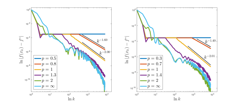
Figure 1: Convergence rate of Algorithm 1 for problem 70 with perturbation 68 ($\tau=1$).

We then consider a sparse and symmetric positive definite matrix $A$ with size $n=1089$. It is obtained from the finite element discretization of the Poisson equation on $[0,1]^{2}$ using piecewise continuous linear polynomials. For Algorithm 1, we set $\mu=\lambda_{\min}(A)$ and $L=\lambda_{\max}(A)$. We consider two kinds of perturbations 68 ($\tau=1$) and 69 and report the results in Fig. 2. For those two cases, the algebraic rate $O(k^{-2p})$ and the linear rate are observed respectively, which agree with Theorems 4.2 and 4.2.

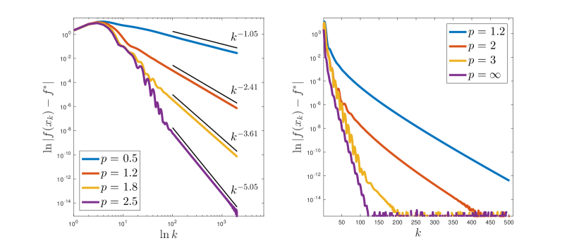
Figure 2: Convergence behaviour of Algorithm 1 for 70 with perturbations 68 (left) and 69 (right).

$\bullet$ Lasso. We then focus on the well-known least absolute shrinkage and selection operator (Lasso) problem

$$\min_{x\in\,{\mathbb{R}}^{n}}\,\frac{1}{2}\left\lVert{Ax-b}\right\rVert^{2}+\rho\left\lVert{x}\right\rVert_{l^{1}},$$ (71)

where $\rho>0,\,b\in\,{\mathbb{R}}^{m},\,A\in\,{\mathbb{R}}^{m\times n}$ and $m\ll n$. We generate $A$ from standard normal distribution and take $b=Ay+e$, where $e$ denotes the noise and $y$ is sparse with $s$ nonzero components. The parameter is chosen as $\rho=0.5$. For Algorithm 1, we set $\mu=0$ and take $L$ as the sum of the diagonal components of $A^{\top}A$. Even though the perturbation 68 is decreasing, the errors in the few initial steps are large. Therefore, to observe the local convergence rate, we set $\tau=1e$-2.

From numerical results in Fig. 3, we find that (i) similar with the previous example (cf. Fig. 1), small $p$ ($<0.5$) cannot promise convergence, and (ii) after a large number of iterations, the perturbations become small and the local decay rate $O(k^{-2})$ arises. This together with the previous test for quadratic programming 70 shows the fast local convergence rate which is better than the global one $O(k^{-\min\{2,2p-2\}})$ given by Theorem 4.1.

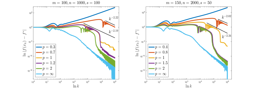
Figure 3: Convergence behaviour of Algorithm 1 for the Lasso problem 71 with perturbation 68 ($\tau=1e$-2).

Appendix A Some Auxiliary Estimates

In this section, we shall present some basic estimates. We first cite an important Gronwall-type inequality; see [42, Proposition 1.2].

Lemma A.1 ([42]).

Let $T>0$ and assume that $y\in C[0,T]$ and $w\in L^{1}(0,T)$. If

$$\frac{1}{2}y^{2}(t)\leqslant\frac{1}{2}c^{2}+\int_{0}^{t}w(s)y(s)\,{\rm d}s,\quad 0<t\leqslant T,$$

where $c\in\mathbb{R}$, then

$$\left\lvert{y(t)}\right\rvert\leqslant\left\lvert{c}\right\rvert+\int_{0}^{t}\left\lvert{w(s)}\right\rvert\mathrm{d}s,\quad 0<t\leqslant T.$$

We also need a discrete version of Lemma A.1, which can be found in [19, Lemma 5.1] or [28, Lemma A.4].

Lemma A.2 ([19]).

Let $\{a_{k}\}_{k=0}^{\infty},\,\{b_{k}\}_{k=0}^{\infty}$ and $\{c_{k}\}_{k=0}^{\infty}$ be three real sequences. If $\{c_{k}\}_{k=0}^{\infty}$ is nondecreasing and for all $k\in\mathbb{N}$,

$$a^{2}_{k}\leqslant c_{k}^{2}+\sum_{i=0}^{j_{k}}a_{i}b_{i},\quad\text{ for some }0\leqslant j_{k}\leqslant k,$$

then it holds that

$$\left\lvert{a_{k}}\right\rvert\leqslant\left\lvert{c_{k}}\right\rvert+\sum_{i=0}^{j_{k}}\left\lvert{b_{i}}\right\rvert,\quad k\in\mathbb{N}.$$

Next,we present an estimate.

Lemma A.3.

Assume that $p\geqslant 0$ and $A>1$, then for all $t>0$,

$$\int_{0}^{t}\frac{A^{s}}{(s+1)^{p}}\,{\rm d}s\leqslant\frac{C_{p}(1+\ln A)}{\left\lvert{\ln A}\right\rvert^{2}}\cdot\frac{A^{t}}{(t+1)^{p}},$$ (72)

where $C_{p}>0$ depends only on $p$.

Proof.

It is trivial to verify 72 with $p=0$, so we consider $p>0$. Define

$$I(t):=\int_{0}^{t}\frac{A^{s+1}}{(s+1)^{p}}\,{\rm d}s,\quad t\geqslant 0.$$

Observing the infinite series expansion

$$A^{s+1}=e^{(s+1)\ln A}=\sum_{n=0}^{\infty}\frac{((s+1)\ln A)^{n}}{n!},$$

which is uniformly convergent over $[0,t]$, we can exchange the order of integral and summation to obtain that

$$I(t)={}\int_{0}^{t}(s+1)^{-p}\sum_{n=0}^{\infty}\frac{((s+1)\ln A)^{n}}{n!}\,{\rm d}s=\sum_{n=0}^{\infty}\frac{(\ln A)^{n}}{n!}\int_{0}^{t}(s+1)^{n-p}\,{\rm d}s.$$ (73)

Consider first that $p\notin\mathbb{N}$, then $n+1-p\neq 0$ for all $n\in\mathbb{N}$. By 73, we have $I(t)=I_{1}+I_{2}$, where

$$\left\{\begin{aligned} I_{1}:={}&\sum_{n=0}^{[p]-1}\frac{(\ln A)^{n}}{n!}\cdot\frac{(t+1)^{n+1-p}-1}{n+1-p},\\ I_{2}:={}&\sum_{n=[p]}^{\infty}\frac{(\ln A)^{n}}{n!}\cdot\frac{(t+1)^{n+1-p}-1}{n+1-p},\end{aligned}\right.$$

where as usual $[p]$ denotes the integer part of $p$. Clearly, $I_{1}$ is nonpositive for $p>1$ and vanishes for $0<p<1$, and the second term $I_{2}$ is bounded by that

$$\small I_{2}={}\frac{1}{(t+1)^{p}\ln A}\sum_{n=[p]}^{\infty}\frac{((t+1)\ln A)^{n+1}}{(n+1)!}\cdot\frac{n+1}{n+1-p}\leqslant{}\frac{1+[p]}{(1+[p]-p)\ln A}\cdot\frac{A^{t+1}}{(t+1)^{p}}.$$ (74)

Hence, we obtain

$$I(t)\leqslant{}\frac{1+[p]}{(1+[p]-p)\ln A}\cdot\frac{A^{t+1}}{(t+1)^{p}}$$ (75)

Then, we consider $p\in\mathbb{N}$. From 73 we obtain that

$$I(t)=I_{2}+I_{3}+\frac{(\ln A)^{p-1}}{(p-1)!}\ln(t+1),$$ (76)

where

$$I_{3}:={}\sum_{n=0}^{p-2}\frac{(\ln A)^{n}}{n!}\cdot\frac{(t+1)^{n+1-p}-1}{n+1-p}.$$

As $I_{3}$ is zero for $p=1$ and nonpositive for $p>1$, we conclude from 74 and 76 that

$$I(t)\leqslant\frac{1+p}{\ln A}\cdot\frac{A^{t+1}}{(t+1)^{p}}+\frac{(\ln A)^{p-1}}{(p-1)!}\ln(t+1).$$

Therefore, applying the elementary inequality

$$\ln(t+1)\leqslant\frac{t+1}{e}\leqslant\frac{(p+1)^{p+1}}{e(e\ln A)^{p+1}}\cdot\frac{A^{t+1}}{(t+1)^{p}}\quad\forall\,t\geqslant 0,$$

and thanks to Stirling’s formula

$$\sqrt{2\pi}(p-1)^{p-\frac{1}{2}}e^{1-p}\leqslant(p-1)!,$$

for all $p\geqslant 2$, we obtain that

$$I(t)\leqslant\frac{C_{p}(1+\ln A)}{\left\lvert{\ln A}\right\rvert^{2}}\cdot\frac{A^{t+1}}{(t+1)^{p}}.$$

This together with 75 proves 72 and completes the proof of this lemma. ∎

A discrete version of Lemma A.3 is given below.

Corollary A.1.

Assume $p\geqslant 0$ and $A>1$, then for all $k\geqslant 1$,

$$\sum_{i=1}^{k}\frac{A^{i}}{(i+1)^{p}}\leqslant\frac{C_{p}(1+\ln A)}{\left\lvert{\ln A}\right\rvert^{2}}\cdot\frac{A^{k+1}}{(k+1)^{p}},$$

where $C_{p}>0$ depends only on $p$.

Proof.

Note that

$$\sum_{i=1}^{k}\frac{A^{i}}{(i+1)^{p}}\leqslant\sum_{i=1}^{k}\int_{i-1}^{i}\frac{A^{s+1}}{(s+1)^{p}}\,{\rm d}s=\int_{0}^{k}\frac{A^{s+1}}{(s+1)^{p}}\,{\rm d}s,$$

and by Lemma A.3 we obtain the desired result. ∎

To the end, we list a lemma that depicts the asymptotic behaviour of some key sequences, and for detailed proof we refer to [14, Lemma B2].

Lemma A.4.

Given $\gamma_{0}>0,\,Q>0$ and $q\geqslant 0$, define $\{\alpha_{k}\}_{k=0}^{\infty}$ and $\{\gamma_{k}\}_{k=0}^{\infty}$ by that

$$\left\{\begin{split}Q\alpha_{k}^{2}={}&\gamma_{k}(1+\alpha_{k}),\,\alpha_{k}>0,\\ \gamma_{k+1}={}&\gamma_{k}+\alpha_{k}(q-\gamma_{k+1}).\end{split}\right.$$

Then we have the following.

• $\gamma_{k}>0,\,\min\{\gamma_{0},q\}\leqslant\gamma_{k}\leqslant\max\{\gamma_{0},q\}$ and $\gamma_{k}\to q$ as $k\to\infty$.

• $\min\{\alpha_{0},\alpha_{q}\}\leqslant\alpha_{k}\leqslant\max\{\alpha_{0},\alpha_{q}\}$ and $\alpha_{k}\to\alpha_{q}$ as $k\to\infty$, where $\alpha_{q}\geqslant 0$ satisfies $Q\alpha_{q}^{2}=q(1+\alpha_{q})$. In addition, if $q=0$, then

  $$\frac{\sqrt{\gamma_{0}}}{\sqrt{\gamma_{0}}\,k+\sqrt{Q}}\leqslant\alpha_{k}\leqslant\frac{2\sqrt{Q}\alpha_{0}}{\sqrt{\gamma_{0}}\,k+2\sqrt{Q}}.$$

• If $q=0$, then for all $k\geqslant 1$,

  $$\frac{Q}{(\sqrt{\gamma_{0}}\,k+\sqrt{Q})^{2}}\leqslant\prod_{i=0}^{k-1}\frac{1}{1+\alpha_{i}}\leqslant\frac{4Q}{(\sqrt{\gamma_{0}}\,k+2\sqrt{Q})^{2}}.$$

References

- [1] Lemaire B. An asymptotical variational principle associated with the steepest descent method for a convex function. J Convex Anal. 1996;3(1):63–70.
- [2] Rockafellar R. Monotone operators and the proximal point algorithm. SIAM J Control Optim. 1976;14(5):877–898.
- [3] Balti M, May R. Asymptotic for the perturbed heavy ball system with vanishing damping term. Evol Equ Control The. 2017;6(2):177–186.
- [4] Haraux A, Jendoubi M. On a second order dissipative ODE in Hilbert space with an integrable source term. Acta Mathematica Scientia. 2012;32(1):155–163.
- [5] Polyak B. Some methods of speeding up the convergence of iteration methods. USSR Computational Mathematics and Mathematical Physics. 1964;4(5):1–17.
- [6] Su W, Boyd S, Candès E. A differential equation for modeling Nesterov’s accelerated gradient method: Theory and insights. Journal of Machine Learning Research. 2016;17:1–43.
- [7] Attouch H, Chbani Z, Riahi H. Rate of convergence of the Nesterov accelerated gradient method in the subcritical case . ESAIM: COCV. 2019;25(2):https://doi.org/10.1051/cocv/2017083.
- [8] Apidopoulos V, Aujol J, Dossal C. The differential inclusion modeling FISTA algorithm and optimality of convergence rate in the case . SIAM J Optim. 2018;28(1):551–574.
- [9] Wibisono A, Wilson A, Jordan M. A variational perspective on accelerated methods in optimization. Proc Nati Acad Sci. 2016;113(47):E7351–E7358.
- [10] Nesterov Y. A method of solving a convex programming problem with convergence rate . Soviet Mathematics Doklady. 1983;27(2):372–376.
- [11] Beck A, Teboulle M. A fast iterative shrinkage-thresholding algorithm for linear inverse problems. SIAM J Imaging Sci. 2009;2(1):183–202.
- [12] Attouch H, Chbani Z, Fadili J, Riahi H. First-order optimization algorithms via inertial systems with Hessian driven damping. Math. Program., hal-02193846. 2020;https://doi.org/10.1007/s10107-020-01591-1.
- [13] Chen L, Luo H. First order optimization methods based on Hessian-driven Nesterov accelerated gradient flow. arXiv: 191209276. 2019;.
- [14] Luo H, Chen L. From differential equation solvers to accelerated first-order methods for convex optimization. Math. Program. 2021;https://doi.org/10.1007/s10107–021–01713–3.
- [15] Siegel J. Accelerated first-order methods: Differential equations and Lyapunov functions. arXiv: 190305671. 2019;.
- [16] Wilson A, Recht B, Jordan M. A Lyapunov analysis of momentum methods in optimization. arXiv: 161102635. 2016;.
- [17] Nesterov Y. Introductory Lectures on Convex Optimization: A Basic Course. Springer Science & Business Media; 2013. (Applied Optimization; 87).
- [18] Jendoubi M, May R. Asymptotics for a second-order differential equation with nonautonomous damping and an integrable source term. Applicable Analysis. 2015;94(2):435–443.
- [19] Attouch H, Chbani Z, Peypouquet J, et al. Fast convergence of inertial dynamics and algorithms with asymptotic vanishing viscosity. Math Program Series B. 2018;168(1-2):123–175.
- [20] Aujol J, Dossal C. Optimal rate of convergence of an ODE associated to the fast gradient descent schemes for . Hal-01547251v2. 2017;.
- [21] Sebbouh O, Dossal C, Rondepierre A. Nesterov’s acceleration and Polyak’s heavy ball method in continuous time: Convergence rate analysis under geometric conditions and perturbations. arXiv:190702710. 2019;.
- [22] Attouch H, Buttazzo G, Michaille G. Variational Analysis in Sobolev and BV Spaces. Society for Industrial and Applied Mathematics; 2014. MOS–SIAM Series on Optimization.
- [23] Paoli L. An existence result for vibrations with unilateral constraints: case of a nonsmooth set of constraints. Math Models Methods Appl Sci. 2000;10(06):815–831.
- [24] Schatzman M. A class of nonlinear differential equations of second order in time. Nonlinear Anal. 1978;2(3):355–373.
- [25] Güler O. New proximal point algorithms for convex minimization. SIAM J Optim. 1992;2(4):649–664.
- [26] Salzo S, Villa S. Inexact and accelerated proximal point algorithms. J Convex Anal. 2012;19(4):1167–1192.
- [27] Villa S, Salzo S, Baldassarre L, et al. Accelerated and inexact forward-backward algorithms. SIAM J Optim. 2013;23(3):1607–1633.
- [28] Aujol J, Dossal C. Stability of over-relaxations for the forward-backward algorithm, application to FISTA. SIAM J Optim. 2015;25(4):2408–2433.
- [29] Schmidt M, Roux N, Bach F. Convergence rates of inexact proximal-gradient methods for convex optimization. Advances in Neural Information Processing Systems. 2011;24:1458–1466.
- [30] Rockafellar R. Convex Analysis. Princeton University Press; 1970.
- [31] Bauschke H, Combettes P. Convex Analysis and Monotone Operator Theory in Hilbert Spaces. New York: Springer Science+Business Media; 2011. CMS Books in Mathematics.
- [32] Brézis H. Functional Analysis, Sobolev Spaces and Partial Differential Equations. New York: Springer; 2011. Universitext.
- [33] Dugundji J. Topology. Boston: Allyn and Bacon, Inc.; 1966. Allyn and Bacon Series in Advanced Mathematics.
- [34] Alber Y, Burachik R, Iusem A. A proximal point method for nonsmooth convex optimization problems in Banach spaces. Abstract and Applied Analysis. 1997;2(1-2):97–120.
- [35] Auslender A. Numerical methods for nondifferentiable convex optimization. In: Cornet B, Nguyen V, Vial J, editors. Nonlinear Analysis and Optimization. Berlin: Springer Berlin Heidelberg; 1987. Mathematical Programming Studies; p. 102–126.
- [36] He B, Yuan X. An accelerated inexact proximal point algorithm for convex minimization. J Optim Theory Appl. 2012;154(2):536–548.
- [37] Monteiro R, Svaiter B. Convergence rate of inexact proximal point methods with relative error criteria for convex optimization. Working paper. 2010;.
- [38] Lin Z, Li H, Fang C. Accelerated Optimization for Machine Learning. Nature Singapore: Springer; 2020.
- [39] d’Aspremont A. Smooth optimization with approximate gradient. SIAM J Optim. 2008;19(3):1171–1183.
- [40] Attouch H, Cabot A, Chbani Z, et al. Inertial forward–backward algorithms with perturbations: Application to Tikhonov regularization. Journal of Optimization Theory and Applications. 2018;179(1):1–36.
- [41] Nesterov Y. Gradient methods for minimizing composite functions. Math Program Series B. 2013;140(1):125–161.
- [42] Barbu V. Differential Equations. Cham: Springer; 2016. Springer Undergraduate Mathematics Series.