MagFace: A Universal Representation for
Face Recognition and Quality Assessment

Abstract

The performance of face recognition system degrades when the variability of the acquired faces increases. Prior work alleviates this issue by either monitoring the face quality in pre-processing or predicting the data uncertainty along with the face feature. This paper proposes MagFace, a category of losses that learn a universal feature embedding whose magnitude can measure the quality of the given face. Under the new loss, it can be proven that the magnitude of the feature embedding monotonically increases if the subject is more likely to be recognized. In addition, MagFace introduces an adaptive mechanism to learn a well-structured within-class feature distributions by pulling easy samples to class centers while pushing hard samples away. This prevents models from overfitting on noisy low-quality samples and improves face recognition in the wild. Extensive experiments conducted on face recognition, quality assessments as well as clustering demonstrate its superiority over state-of-the-arts. The code is available at https://github.com/IrvingMeng/MagFace.

1 Introduction

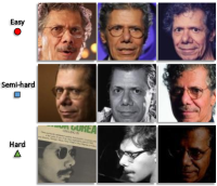
(a)

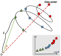
(b)

Figure 1: MagFace learns for (a) in-the-wild faces (b) a universal embedding by pulling the easier samples closer to the class center and pushing them away from the origin $o$. As shown in our experiments and supported by mathematical proof, the magnitude $l$ before normalization increases along with feature’s cosine distance to its class center, and therefore reveals the quality for each face. The larger the $l$, the more likely the sample can be recognized.

Recognizing face in the wild is difficult mainly due to the large variability exhibited by face images acquired in unconstrained settings. This variability is associated to the image acquisition conditions (such as illumination, background, blurriness, and low resolution), factors of the face (such as pose, occlusion and expression) or biases of the deployed face recognition system [36]. To cope with these challenges, most relevant face analysis system under unconstrained environment (, surveillance video) consists of three stages: 1) face acquisition to select from a set of raw images or capture from video stream the most suitable face image for recognition purpose; 2) feature extraction to extract discriminative representation from each face image; 3) facial application to match the reference image towards a given gallery or cluster faces into groups of same person.

To acquire the optimal reference image in the first stage, a technique called face quality assessment [4, 26] is often employed on each detected face. Although the ideal quality score should be indicative of the face recognition performance, most of early work [1, 2] estimates qualities based on human-understandable factors such as luminances, distortions and pose angles, which may not directly favor the face feature learning in the second stage. Alternatively, learning-based methods [4, 15] train quality assessment models with artificially or human labelled quality values. Theses methods are error-prone as there lacks of a clear definition of quality and human may not know the best characteristics for the whole systems.

To achieve high end-to-end application performances in the second stage, various metric-learning [27, 30] or classification losses [48, 25, 20, 13, 40, 9, 5] emerged in the past few years. These works learn to represent each face image as a deterministic point embedding in the latent space regardless of the variance inherent in faces. In reality, however, low-quality or large-pose images like Fig. 1a widely exist and their facial features are ambiguous or absent. Given these challenges, a large shift in the embedded points is inevitable, leading to false recognition. For instance, performance reported by prior state-of-the-art [29] on IJB-C is much lower than LFW. Recently, confidence-aware methods [29, 7] propose to represent each face image as a Gaussian distribution in the latent space, where the mean of the distribution estimates the most likely feature values while the variance shows the uncertainty in the feature values. Despite the performance improvement, these methods seek to separate the face feature learning from data noise modeling. Therefore, additional network blocks are introduced in the architecture to compute the uncertainty level for each image. This complicates the training procedure and adds computational burden in inference. In addition, the uncertainty measure cannot be directed used in conventional metrics for comparing face features.

This paper proposes MagFace to learn a universal and quality-aware face representation. The design of MagFace follows two principles: 1) Given the face images of the same subject but in different levels of quality (, Fig. 1a), it seeks to learn a within-class distribution, where the high-quality ones stay close to the class center while the low-quality ones are distributed around the boundary. 2) It should pose the minimum cost for changing existing inference architecture to measure the face quality along with the computation of face feature. To achieve the above goals, we choose magnitude, the independent property to the direction of the feature vector, as the indicator for quality assessment. The core objective of MagFace is to not only enlarge inter-class distance, but also maintain a cone-like within-class structure like Fig. 1b, where ambiguous samples are pushed away from the class centers and pulled to the origin. This is realized by adaptively down-weighting ambiguous samples during training and rewarding the learned feature vector with large magnitude in the MagFace loss. To sum up, MagFace improves previous work in two aspects:

1. For the first time, MagFace explores the complete set of two properties associated with feature vector, direction and magnitude, in the problem of face recognition while previous works often neglect the importance of the magnitude by normalizing the feature. With extensive experimental study and solid mathematical proof, we show that the magnitude can reveal the quality of faces and can be bundled with the characteristics of recognition without any quality labels involved.

2. MagFace explicitly distributes features structurally in the angular direction (as shown in Fig. 1b). By dynamically assigning angular margins based on samples’ hardness for recognition, MagFace prevents model from overfitting on noisy and low-quality samples and learns a well-structured distributions that are more suitable for recognition and clustering purpose.

2 Related Works

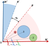
(a)

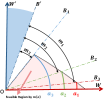
(b)

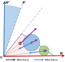
(c)

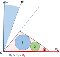
(d)

Figure 2: Geometrical interpretation of the feature space (without normalization) optimized by ArcFace and MagFace. (a) Two-class distributions optimized by ArcFace, where $w$ and $w^{\prime}$ are the class centers and their decision boundaries $B$ and $B^{\prime}$ are separated by the additive margin $m$. Circle 1, 2, 3 represent three types samples of class $w$ with descending qualities. (b) MagFace introduces $m(a_{i})$ which dynamically adjust boundaries based on feature magnitudes, and ends to a new feasible region. (c) Effects of $g(a_{i})$ and $m(a_{i})$. (d) Final feature distributions of our MagFace. Best viewed in color.

2.1 Face Recognition

Recent years have witnessed the breakthrough of deep convolutional face recognition techniques. A number of successful systems, such as DeepFace [35], DeepID [33], FaceNet [27] have shown impressive performance on face identification and verification. Apart from the large-scale training data and deep network architectures, the major advance comes from the evolution of training losses for CNN. Most of early works rely on metric-learning based loss, including contrastive loss [8], triplet loss [27], n-pair loss [30], angular loss [41], . Suffering from the combinatorial explosion in the number of face triplets, embedding-based method is usually inefficient in training on large-scale dataset. Therefore, the main body of research in deep face recognition has focused on devising more efficient and effective classification-based loss. Wen et al. [44] develop a center loss to learn centers for each identity to enhance the intra-class compactness. $L_{2}$-softmax [25] and NormFace [39] study the necessity of the normalization operation and applied $L_{2}$ normalization constraint on both features and weights. From then on, several angular margin-based losses, such as SphereFace [20], AM-softmax [38], SV-AM-Softmax [42], CosFace [40], ArcFace [9], progressively improve the performance on various benchmarks to the newer level. More recently, AdaptiveFace [19], AdaCos [49] and FairLoss [18] introduce adaptive margin strategy to automatically tune hyperparameters and generate more effective supervisions during training. Compared to our method, all these work tend to suppress the effect of magnitude in the loss by normalizing the feature vector.

2.2 Face Quality Assessment

Face image quality is an important factor to enable high-performance face recognition systems [4]. Traditional methods, such as ISO/IEC 19794-5 standard [1], ICAO 9303 standard [2], Brisque [31], Niqe [23] and Piqe [37], describe qualities from image-based aspects (, distortion, illumination and occlusion) or subject-based measures (, accessories). Learning-based approaches such as FaceQNet [15] and Best-Rowden [4] regress qualities by networks trained on human-assessed and similarity-based labels. However, these quality labels are error-prone as human may not know the best characteristics for the recognition system and therefore cannot consider all proper factors. Recently, several uncertainty-based methods are proposed to express face qualities by the uncertainties of features. SER-FIQ [36] forwards an image to a network with dropout several times and measures face quality by the variation of extracted features. Confidence-aware face recognition methods [29, 7] propose to represent each face image as a Gaussian distribution in the latent space and learn the uncertainty in the feature values. Although these methods work in an unsupervised manner like ours, they require additional computational costs or network blocks, which complicate their usage in conventional face systems.

2.3 Face Clustering

Face clustering exploits unlabeled data to cluster them into pseudo classes. Traditional clustering methods usually work in an unsupervised manner, such as K-means [21]. DBSCAN [11] and hierarchical clustering. Several supervised clustering methods based on graph convolutional network (GCN) are proposed recently. For example, L-GCN [43] performs reasoning and infers the likelihood of linkage between pairs in the sub-graphs. Yang et al. [46] designs two graph convolutional networks, named GCN-V and GCN-E, to estimate the confidence of vertices and the connectivity of edges, respectively. Instead of developing clustering methods, we aim at improving feature distribution structure for clustering.

3 Methodology

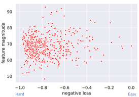
(a) Softmax

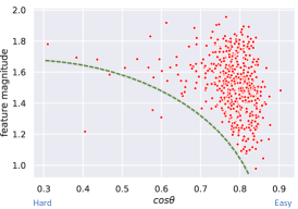
(b) ArcFace

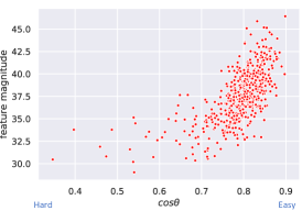
(c) MagFace

Figure 3: Visualization of feature magnitudes and difficulties for recognition. Models are trained on MS1M-V2 [14, 9] and 512 samples of the last iteration are used for visualization. Negative losses are used to reveal the hardness for Softmax while we use cosine value of $\theta$ (angle between a feature and its class center) for ArcFace and MagFace.

In this section, we first review the definition of ArcFace [9], one of the most popular losses used in face recognition. Based on the analysis of ArcFace, we then derive the objective and prove the key properties for MagFace. In the end, we compare softmax and ArcFace with MagFace from the perspective of feature magnitude.

3.1 ArcFace Revisited

Training loss plays an important role in face representation learning. Among the various choices (see [10] for a recent survey), ArcFace [9] is perhaps the most widely adopted one in both academy and industry application due to its easiness in implementation and state-of-the-art performance on a number of benchmarks. Suppose that we are given a training batch of $N$ face samples $\{f_{i},y_{i}\}_{i=1}^{N}$ of $n$ identities, where $f_{i}\in\mathbb{R}^{d}$ denotes the $d$-dimensional embedding computed from the last fully connected layer of the neural networks and $y_{i}=1,\cdots,n$ is its associated class label. ArcFace and other variants improve the conventional softmax loss by optimizing the feature embedding on a hypersphere manifold where the learned face representation is more discriminative. By defining the angle $\theta_{j}$ between $f_{i}$ and $j$-th class center $w_{j}\in\mathbb{R}^{d}$ as $w_{j}^{T}f_{i}=\|w_{j}\|\|f_{i}\|\cos\theta_{j}$, the objective of ArcFace [9] can be formulated as

$$L=-\frac{1}{N}\sum_{i=1}^{N}\log\frac{e^{s\cos{(\theta_{y_{i}}+m)}}}{e^{s\cos{(\theta_{y_{i}}+m)}}+\sum_{j\neq y_{i}}e^{s\cos{\theta_{j}}}},$$ (1)

where $m>0$ denotes the additive angular margin and $s$ is the scaling parameter.

Despite its superior performances on enforcing intra-class compactness and inter-class discrepancy, the angular margin penalty $m$ used by ArcFace is quality-agnostic and the resulting structure of the within-class distribution could be arbitrary in unconstrained scenarios. For example, let us consider the scenario illustrated in Fig. 2a, where we have face images of the same class in three levels of qualities indicated by the circle sizes: the larger the radius, the more uncertain the feature representation and the more difficulty the face can be recognized. Because ArcFace employs a uniform margin $m$, each image in one class shares the same decision boundary, , $B:\cos(\theta+m)=\cos(\theta^{\prime})$ with respect to the neighbor class. The three types of samples can stay at arbitrary location in the feasible region (shading area in Fig. 2a) without any penalization by the angular margin. This leads to unstable within-class distribution, , the high-quality face (type 1) stay along the boundary $B$ while the low-quality ones (type 2 and 3) are closer to the center $w$. This unstableness can hurt the performances on in-the-wild recognition as well as other facial application such as face clustering. Moreover, hard and noisy samples are over-weighted as they are hard to stay in the feasible area and the models may overfit to them.

3.2 MagFace

Based on the above analysis, previous cosine-similarity-based face recognition loss lacks more fine-grained constraint beyond a fixed margin $m$. This leads to unstable within-class structure especially in the unconstrained case (, Fig. 2a) where the variability of each subject’s faces is large. To address the aforementioned problem, this section proposes MagFace, a novel framework to encode quality measure into the face representation. Unlike previous work [29, 7] that call for additional uncertainty term, we pursue a minimalism design by optimizing over the magnitude $a_{i}=\|f_{i}\|$ without normalization of each feature $f_{i}$. Our design has two major advantages: 1) We can keep using the cosine-based metric that has been widely adopted by most existing inference systems; 2) By simultaneously enforcing its direction and magnitude, the learned face representation is more robust to the variability of faces in the wild. To our best understanding, this is the first work to unify the feature magnitude as quality indicator in face recognition.

Before defining the loss, let us first introduce two auxiliary functions related to $a_{i}$, the magnitude-aware angular margin $m(a_{i})$ and the regularizer $g(a_{i})$. The design of $m(a_{i})$ follows a natural intuition: for high-quality samples $x_{i}$, they should concentrate in a small region around the cluster center $w$ with high certainty. By assuming a positive correlation between the magnitude and quality, we thereby penalize more on $x_{i}$ in terms of $m(a_{i})$ if its magnitude $a_{i}$ is large. To have a better understanding, Fig. 2b visualizes the margins $m(a_{i})$ corresponding to different magnitude values. In contrast to ArcFace (Fig. 2a), the feasible region defined by $m(a_{i})$ has a shrinking boundary with respect to feature magnitude towards the class center $w$. Consequently, this boundary pulls the low-quality samples (circle 2 and 3 in Fig. 2c) to the origin where they have lower risk to be penalized. However, the structure formed solely by $m(a_{i})$ is unstable for high-quality samples like circle 1 in Fig. 2c as they have large freedom moving inside the feasible region. We therefore introduce the regularizer $g(a_{i})$ that rewards sample with large magnitude. By designing $g(a_{i})$ as a monotonically decreasing convex function with respect to $a_{i}$, each sample would be pushed towards the boundary of the feasible region and the high-quality ones (circle 1) would be dragged closer to the class center $w$ as shown in Fig. 2d. In a nutshell, MagFace extends ArcFace (Eq. 1) with magnitude-aware margin and regularizer to enforce higher diversity for inter-class samples and similarity for intra-class samples by optimizing:

$$L_{Mag} =\frac{1}{N}\sum_{i=1}^{N}L_{i},\quad\text{where}$$ (2)

$$L_{i} =-\log\frac{e^{s\cos{(\theta_{y_{i}}+m(a_{i}))}}}{e^{s\cos{(\theta_{y_{i}}+m(a_{i}))}}+\sum_{j\neq y_{i}}e^{s\cos{\theta_{j}}}}+\lambda_{g}g(a_{i}).$$

The hyper-parameter $\lambda_{g}$ is used to trade-off between the classification and regularization losses.

The design of MagFace not only follows intuitive motivations, but also yields result with theoretical guarantees. Assuming the magnitude $a_{i}$ is bounded in $[l_{a},u_{a}]$, where $m(a_{i})$ is a strictly increasing convex function, $g(a_{i})$ is a strictly decreasing convex function and $\lambda_{g}$ is large enough, we can prove (see detailed requirements and proofs in the supplementary) that the following two properties of MagFace loss always hold when optimizing $L_{i}$ over $a_{i}$:

Property of Convergence.

For $a_{i}\in[l_{a},u_{a}]$, $L_{i}$ is a strictly convex function which has a unique optimal solution $a_{i}^{*}$.

Property of Monotonicity.

The optimal $a_{i}^{*}$ is monotonically increasing as the cosine-distance to its class center decreases and the cos-distances to other classes increase.

The property of convergence guarantees the unique optimal solution for $a_{i}$ as well as the fast convergence. The property of monotonicity states that the feature magnitudes reveal the difficulties for recognition, therefore can be treated as a metric for face qualities.

3.3 Analysis on Feature Magnitude

To better understand the effect of the MagFace loss, we conduct experiments on the widely used MS1M-V2 [9] dataset and investigate for the training examples at convergence the relation between the feature magnitude and their similarity with class center as shown in Fig. 3.

Softmax. The classical softmax-based loss underlies the objective of the pioneer work [35, 34] on deep face recognition. Without explicit constraint on magnitude, the value of the negative loss for each sample is almost independent to its magnitude as observed from Fig. 3a. As pointed in [25, 39], softmax tends to create a radial feature distribution because softmax loss acts as the soft version of max operator and scaling the feature magnitude does not affect the assignment of its class. To eliminate this effect, [25, 39] suggest that using normalized feature would benefit the task.

ArcFace. ArcFace can be considered as a special case of MagFace when $m(a_{i})=m$ and $g(a_{i})=0$. As shown in Fig. 3b, high-quality samples with large similarity $\cos(\theta)$ to class center yield large variation in magnitude. This evidence echos our motivation on the unstable structure defined by a fixed angular margin in ArcFace for easy samples. On the other hand, for low-quality samples that are difficult to be recognized ($\cos(\theta)$ is small), the fixed angular margin determines the magnitude needs to be large enough in order to fit inside the feasible region (Fig. 2a). Therefore, there is a decreasing low bound for feature magnitudes the quality of face as indicated by the dash line in Fig. 3b.

MagFace. In contrast to ArcFace, our MagFace optimizes the feature with adaptive margin and regularization based on its magnitude. Under this loss, it is clear to observe from Fig. 3c that there is a strong correlation between the feature magnitudes and their cosine similarities with class center. Those examples at the upper-right corner are the most high-quality ones. As the magnitude becomes smaller, the examples are more deviated from the class center. This distribution strongly supports the fact that the feature magnitude learned by MagFace is a good metric for face quality.

4 Experiments

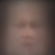
(a)

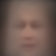
(b)

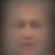
(c)

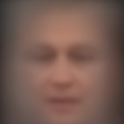
(d)

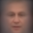
(e)

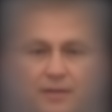
(f)

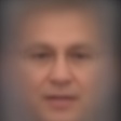
(g)

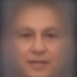
(h)

Figure 4: Visualization of the mean faces of 100k images sampled from the IJB-C dataset. Each mean face corresponds to a group of faces based on the magnitude level of the features learned by MagFace.

In this section, we examine the proposed MagFace on three important face tasks: face recognition, quality assessment and face clustering. Sec. C in the supplementary presents the ablation study on relationships between margin distributions and recognition performances.

4.1 Face Recognition

Datasets. The original MS-Celeb-1M dataset [14] contains about 10 million images of 100k identities. However, it consists of a great many noisy face images. Instead, we employ MS1M-V2 [9] (5.8M images, 85k identities) as our training dataset. For evaluation, we adopt LFW [16], CFP-FP [28], AgeDB-30 [24], CALFW [51], CPLFW [50], IJB-B [45] and IJB-C [22] as the benchmarks. All the images are aligned to $112\times 112$ by following the setting in ArcFace.

Baselines. We re-implement state-of-the-art baselines including Softmax, SV-AM-Softmax [42], SphereFace [20], CosFace [40], ArcFace [9]. ResNet100 is equipped as the backbone. We use the recommended hyperparameters for each model, , $s=64$, $m=0.5$ for ArcFace.

Training. We train models on 8 1080Tis by stochastic gradient descent. The learning rate is initialized from 0.1 and divided by 10 at 10, 18, 22 epochs, and we stop the training at the 25th epoch. The weight decay is set to 5e-4 and the momentum is 0.9. We only augment training samples by random horizontal flip. For MagFace, we fix the upper bound and lower bound of the magnitude as $l_{a}=10,u_{a}=110$. $m(a_{i})$ is chosen to be a linear function and $g(a_{i})$ as a hyperbola. For detailed definition of $m(a_{i})$, $g(a_{i})$ and $\lambda_{g}$, please refer to Sec. B2 in the supplementary. In the end, our mean margin as well as other hyperparameters are all consistent with ArcFace.

Test. During testing, cosine distance is used as metric on comparing 512-D features. For evaluations on IJB-B/C, one identity can have multiple images. The common way to represent for an identity is to sum up the normalized feature $f_{i}^{norm}=\frac{f_{i}}{\|f_{i}\|}$ of each image and then normalize the embedding for comparisons, , $f=\frac{\sum_{i}f_{i}^{norm}}{\|\sum_{i}f_{i}^{norm}\|}$. One benefit of MagFace is that we can assign quality-aware weight $\|f_{i}\|$ to each normalized feature $f_{i}^{norm}$. Therefore, we further evaluate “MagFace+” in Tab. 2 by computing the identity embedding as $f_{+}=\frac{\sum_{i}f_{i}}{\|\sum_{i}f_{i}\|}$.

Method	LFW	CFP-FP	AgeDB-30	CALFW	CPLFW
Softmax	99.70	98.20	97.72	95.65	92.02
SV-AM-Softmax [42]	99.50	95.10	95.68	94.38	89.48
SphereFace [20]	99.67	96.84	97.05	95.58	91.27
CosFace [40]	99.78	98.26	98.17	96.18	92.18
ArcFace [9]	99.81	98.40	98.05	95.96	92.72
MagFace	99.83	98.46	98.17	96.15	92.87

Table 1: Verification accuracy (%) on easy benchmarks.

Results on LFW, CFP-FP, AgeDB-30, CALFW and CPLFW. We directly use the aligned images and protocols adopted by ArcFace [9] and present our results in Tab. 1. We note that performances are almost saturated. Compared to CosFace which is the second best baseline, ArcFace achieves $0.03\%,0.14\%,0.54\%$ improvement on LFW, CFP-FP and CPLFW, while drops $0.12\%,0.22\%$ on AgeDB-30 and CALFW. MagFace obtains the overall best results and surpasses ArcFace by $0.02\%$, $0.06\%$, $0.12\%$, $0.19\%$ and $0.15\%$ on five benchmarks respectively.

Method	IJB-B (TAR@FAR)			IJB-C (TAR@FAR)
	1e-6	1e-5	1e-4	1e-6	1e-5	1e-4
VGGFace2* [6]	-	67.10	80.00	-	74.70	84.00
CenterFace* [44]	-	-	-	-	78.10	85.30
CircleLoss* [32]	-	-	-	-	89.60	93.95
ArcFace* [9]	-	-	94.20	-	-	95.60
Softmax	46.73	75.17	90.06	64.07	83.68	92.40
SV-AM-Softmax [42]	29.81	69.25	84.79	63.45	80.30	88.34
SphereFace [20]	39.40	73.58	89.19	68.86	83.33	91.77
CosFace [40]	40.41	89.25	94.01	87.96	92.68	95.56
ArcFace [9]	38.68	88.50	94.09	85.65	92.69	95.74
MagFace	40.91	89.88	94.33	89.26	93.67	95.81
MagFace+	42.32	90.36	94.51	90.24	94.08	95.97

Table 2: Verification accuracy (%) on difficult benchmarks. “*” indicates the result quoted from the original paper.

Results on IJB-B/IJB-C. The IJB-B dataset contains 1,845 subjects with 21.8K still images and 55K frames from 7,011 videos. As the extension of IJB-B, the IJB-C dataset covers about 3,500 identities with a total of 31,334 images and 117,542 unconstrained video frames. In the 1:1 verification, the number of positive/negative matches are 10k/8M in IJB-B and 19k/15M in IJB-C. We report the TARs at FAR=1e-6, 1e-5 and 1e-4 as shown in Tab. 2.

Our implemented ArcFace is on par with the original paper, , our TARs at FAR=1e-4 differ from the authors by $-0.11\%$ and $+0.14\%$ on IJB-B and IJB-C respectively. Compared to baselines, our MagFace remains the top at all FAR criteria except for FAR=1e-6 on IJB-B as the TAR is very sensitive to the noise when the number of FP is tiny. Compared to CosFace, MagFace gains $0.50\%,0.63\%,0.32\%$ on IJB-B at TAR@FAR=1e-6, 1e-5, 1e-4 and $1.30\%,0.99\%,0.25\%$ on IJB-C. Compared to ArcFace, improvements are of $2.23\%,1.38\%,0.24\%$ on IJB-B and $3.61\%,0.98\%,0.07\%$ on IJB-C respectively. This result demonstrates the superiority of MagFace on more challenging benchmarks. It is worth to mention that when multiple images existed for one identity, the average embedding can be further improved by aggregating features weighted by magnitudes. For instance, MagFace+ outperforms MagFace by $1.41\%/0.98\%$ at FAR=1e-6, $0.48\%/0.41\%$ at FAR=1e-5 and $0.18\%/0.16\%$ at FAR=1e-4.

4.2 Face Quality Assessment

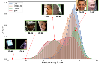
Figure 5: Distributions of magnitudes on different datasets.

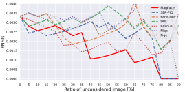
(a) LFW - ArcFace

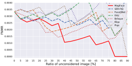
(b) LFW - MagFace

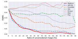
(c) CFP-FP - ArcFace

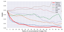
(d) CFP-FP - MagFace

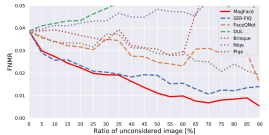
(e) AgeDB-30 - ArcFace

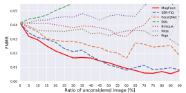
(f) AgeDB-30 - MagFace

Figure 6: Face verification performance for the predicted face quality values with two evaluation models (ArcFace and MagFace). The curves show the effectiveness of rejecting low-quality face images in terms of false non-match rate (FNMR). Best viewed in color.

In this part, we investigate the qualitative and quantitative performance of the pre-trained MagFace model mentioned in Tab. 2 for quality assessment.

Visualization of the mean face. We first sample 100k images form IJB-C database and divide them into 8 groups based on feature magnitudes. We visualize the mean faces of each group in Fig. 4. It can be seen that when magnitude increases, the corresponding mean face reveals more details. This is because high-quality faces are inclined to be more frontal and distinctive. This implies the magnitude of MagFace feature is a good quality indicator.

Sample distribution of datasets. Fig. 5 plots the sample histograms of different benchmarks with respect to MagFace magnitudes. We observe that LFW is the least noisy one where most samples are of large magnitudes. Due to the larger age variation, the distribution of AGEDB-30 slightly shifts left compared to LFW. For CFP-FP, there are two peaks at the magnitude around 28 and 34, corresponding to the frontal and profile faces respectively. Given the large variations in face qualities, we can conclude IJB-C is much more challenging than other benchmarks. For images (more examples can be found in the supplementary) with magnitudes $a\simeq 15$, there are no faces or very noisy faces to observe. When feature magnitudes increase from 20 to 40, there is a clear trend that the face changes from profile, blurred and occluded, to more frontal and distinctive. Overall, this figure convinces us that MagFace is an effective tool to rank face images according to their qualities.

Baselines. We choose six baselines of three types for quantitative quality evaluation. Brisque [31], Niqe [23] and Piqe [37] are image-based quality metrics. FaceQNet [15] and SER-FIQ [36] are face-based ones. For FaceQNet, we adopt the released models by the authors. For SER-FIQ, we use the “same model” version which yields the best performance in the paper. Following the authors’ setting, we set $m=100$ to forward each image 100 times with drop-out active in inference. As a related work, we re-implement the recent DUL [7] method that can estimate uncertainty along with the face feature.

Evaluation metric. Following previous work [12, 36, 4], we evaluate the quality assessment on LFW/CFP-FP/AgeDB via the error-versus-reject curves, where images with the lowest predicted qualities are unconsidered and error rates are calculated on the remaining images. Error-versus-reject curve indicates good quality estimation when the verification error decreases consistently while increasing the ratio of unconsidered images. To compute the feature for verification, we adopt the ArcFace* as well as our MagFace models in Tab. 2.

Results on face verification. Fig. 6 shows the error-versus-reject curves of different quality methods in terms of false non-match rate (FNMR) reported at false match rate (FMR) threshold of 0.001. Overall, we have two high-level observations. 1) The curves on CFP-FP and AgeDB-30 are much more smooth than the ones obtained on LFW. This is because CFP-FP and AgeDB-30 consist of faces with larger variations in pose and age. Effectively dropping low-quality faces can benefit the verification performance more on these two benchmarks. 2) No matter computing the feature from ArcFace (left column) or MagFace (right column), the curves corresponding to MagFace magnitude are consistently the lowest ones across different benchmarks. This indicates that the performance of MagFace magnitude as quality generalizes well across datasets as well as face features. We then analyze the quality performance of each type of methods. 1) The image-based quality metrics (Brisque [31], Niqe [23], Piqe [37]) lead to relatively higher errors in most cases as the image quality alone is not suitable for generalized face quality estimation. Factors of the face (such as pose, occlusions, and expressions) and model biases are not covered by these algorithms and might play an important role for face quality assessment. 2) The face-based methods (FaceQNet [15] and SER-FIQ [36]) outperforms other baselines in most cases. In particular, SER-FIQ is more effective than FaceQNet in terms of the verification error rates. This is due to the fact that SER-FIQ is built on top of the deployed recognition model so that its prediction is more suitable for the verification task. However, SEQ-FIQ takes a quadratic computational cost the number of sub-networks $m$ randomly sampled using dropout. In contrary, the neglectable overhead of computing magnitude makes the proposed MagFace more practical in many real-time scenarios. Moreover, the training of MagFace does not require explicit labeling of face quality, which is not only time consuming but also error-prone to obtain. 3) At last, the uncertainty method (DUL) performs well on CFP-FP but yields more verification errors on AgeDB-30 when the proportion of unconsidered images is increased. This may indicate that the Gaussian assumption of data variance in DUL is over-simplified such that the model cannot generalize well to different kinds of quality factors.

4.3 Face Clustering

In this section, we conduct experiments on face clustering to further investigate the structure of feature representations learned by MagFace.

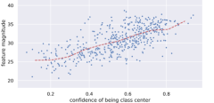
Figure 7: Visualization of MagFace magnitudes of 500 samples from IJB-B-1845 their confidences of being class centers.

Baselines. We compare the performances of MagFace and ArcFace by integrating their features with various clustering methods. For fair comparisons, we constrain hyperparameters of the two models to be consistent (, s=64, mean margin 0.5) during training. Four clustering methods are used in the evaluation: K-means [21], AHC [17], DBSCAN [11] and L-GCN [43]. For non-deterministic algorithms (K-means and AHC), we report the average results from 10 runs. For L-GCN, we train the model on CASIA-WebFace [47] (0.5M images from 10k individuals) and follow the recommended settings in the paper [43].

Benchmarks. We adopt the IJB-B [45] dataset as the benchmark as it contains a clustering protocol of seven sub-tasks varying in the number of ground truth identities. Following [43], we evaluate on three largest sub-tasks where the numbers of identities are 512, 1,024 and 1,845, and the numbers of samples are 18,171, 36,575 and 68,195, respectively. Normalized mutual information (NMI) and BCubed F-measure [3] are employed as the evaluation metrics.

Method	Net	IJB-B-512		IJB-B-1024		IJB-B-1845
		F	NMI	F	NMI	F	NMI
K-means [21]	ArcFace	66.70	88.83	66.82	89.48	66.93	89.88
	MagFace	66.75	88.86	67.33	89.62	67.06	89.96
AHC [17]	ArcFace	69.72	89.61	70.47	90.54	70.66	90.90
	MagFace	70.24	89.99	70.68	90.67	70.98	91.06
DBSCAN [11]	ArcFace	72.72	90.42	72.50	91.15	73.89	91.96
	MagFace	73.13	90.61	72.68	91.30	74.26	92.13
L-GCN [43]	ArcFace	84.92	93.72	83.50	93.78	80.35	92.30
	MagFace	85.27	93.83	83.79	94.10	81.58	92.79

Table 3: F-score (%) and NMI (%) on clustering benchmarks.

Results. Tab. 3 summarizes the clustering results. We can observe that with stronger clustering methods from K-means to L-GCN, the overall clustering performance can be improved. For any combination of clustering and protocol, MagFace always achieves better performance than ArcFace in terms of both F-score and NMI metrics. This consistent superiority demonstrates the MagFace feature is more suitable for clustering. Notice that we keep the same hyperparameters for clustering. The improvement of using MagFace must come from its better within-class feature distribution, where the high-quality samples around the class center are more likely to be separated across different classes.

We further explore the relationship between feature magnitudes and the confidences of being class centers. Following the idea mentioned in [46], the confidence of being a class center for each sample is estimated based on its neighbor structure defined by face features. The samples with dense and pure local connection have high confidence, while those with sparse connections or residing in the boundary among several clusters have low confidence. From Fig. 7, it is easy to observe that the MagFace magnitude is positively correlated with confidence of class center on the IJB-B-1845 benchmark. This result reflects that the MagFace feature exhibits the expected within-class structure, where high quality samples distribute around class center while low quality ones are far away from the center.

5 Conclusion

In this paper, we propose MagFace to learn unified features for face recognition and quality assessment. By pushing ambiguous samples away from class centers, MagFace improves the within-class feature distribution from previous margin-based work for face recognition. The adequate theoretical and experimental results convince that MagFace can simultaneously access quality for the input face image. As a general framework, MagFace can be potentially extended to benefit other classification tasks such as fine-grained object recognition, person re-identification. Moreover, the proposed principle of exploring feature magnitude paves the way to estimate quality for other objects, , person body in reid or action snippet in activity classification.

Method	Hyperparameters					Margin			CFP-FP	IJB-C (TAR@FAR)
	$l_{m}$	$u_{m}$	$\lambda_{g}$	$l_{a}$	$u_{a}$	mean	max	min		1e-6	1e-5	1e-4	1e-3
ArcFace	-	-	-	-	-	0.50	-	-	97.32	83.88	91.59	95.00	96.86
MagFace	0.45	0.65	35	10	110	0.50	0.49	0.52	97.23	81.12	91.44	94.95	96.96
	0.40	0.80	35	10	110	0.50	0.46	0.53	97.47	85.82	92.06	95.12	96.92
	0.35	1.00	35	10	110	0.50	0.42	0.54	97.40	84.35	91.65	95.05	97.02
	0.25	1.60	35	10	110	0.50	0.35	0.61	97.30	81.64	91.09	94.91	96.87

Table 4: Verification accuracy (%) on CFP-FP and IJB-C with different distributions of margins. Backbone network: ResNet50.

Appendix A Proofs for MagFace

Recall the MagFace loss for a sample $i$ is

Let $A(a_{i})=s\cos(\theta_{y_{i}}+m(a_{i}))$ and $B=\sum_{j=1,j\neq y_{i}}^{n}e^{s\cos{\theta_{j}}}$ and rewrite the loss as

We first introduce and prove Lemma 1.

Lemma 1.

Assume that $f_{i}$ is top-k correctly classified and $m(a_{i})\in[0,\pi/2]$. If the number of identities $n$ is much larger than $k$ (i.e., $n\gg k$), the probability of $\theta_{y_{i}}+m(a_{i})\in[0,\pi/2]$ approaches 1.

Proof.

Denote the angle between feature $f_{i}$ and center class $W_{j},j\in\{1,\cdots,n\}$ as $\theta_{j}$. Assuming the distribution of $\theta_{j}$ is uniform, it’s easy to prove $P\left(\theta_{j}+m(a_{i})\in[0,\pi/2]\right)=\frac{\pi/2-m(a_{i})}{\pi}$. Let $p=\frac{\pi/2-m(a_{i})}{\pi}$. If $f_{i}$ is top-k correctly classified, the probability of $\theta_{y_{i}}+m(a_{i})\in[0,\pi/2]$ is the same as the probability of there are at least k $\theta$ to satisfy $\theta+m(a_{i})\in[0,\pi/2]$. Then the probability is

When $n$ is a large integer and $n\gg k$, each $\binom{n}{i}p^{i}(1-p)^{(n-i)},i=1,2,\cdots k-1$ converges to 0. Therefore, probability of $\theta_{y_{i}}+m(a_{i})\in[0,\pi/2]$ approaches 1. ∎

Lemma 1 is fundamental for the following proofs. The number of identities is large in real-world applications (e.g., 3.8M for MS1Mv2 [14, 9]). Therefore, the probability of $\theta_{y_{i}}+m(a_{i})\in[0,\pi/2]$ approaches 1 in most cases.

A.1 Requirements for MagFace

In MagFace, $m(a_{i}),g(a_{i}),\lambda_{g}$ are required to have the following properties:

1. $m(a_{i})$ is an increasing convex function in $[l_{a},u_{a}]$ and $m^{\prime}(a_{i})\in(0,K]$, where $K$ is a upper bound;

2. $g(a_{i})$ is a strictly convex function with $g^{\prime}(u_{a})=0$;

3. $\lambda_{g}\geq\frac{sK}{-g^{\prime}(l_{a})}$.

A.2 Proof for Property of Convergence

We prove the property of convergence by showing the strict convexity of the function $L_{i}$ (Property 5) and the existence of the optimum (Property 6).

Property 1.

For $a_{i}\in[l_{a},u_{a}]$, $L_{i}$ is a strictly convex function of $a_{i}$.

Proof.

The first and second deriviates of $A(a_{i})$ are

According to Lemma 1, we have $\cos(\theta_{y_{i}}+m(a_{i}))\geq 0$ and $\sin(\theta_{y_{i}}+m(a_{i}))\geq 0$. Because we define $m(a_{i})$ to be convex and $g(a_{i})$ to be strictly convex for $a_{i}\in[l_{a},u_{a}]$, $m^{\prime\prime}(a_{i})\geq 0$ and $g^{\prime\prime}(a_{i})>0$ always hold. Therefore, $A^{\prime\prime}(a_{i})\leq 0$.

The first and second order derivatives of the loss $L_{i}$ are

As $B>0,e^{A(a_{i})}+B>0$, it’s easy to prove that first two parts of $\frac{\partial^{2}L_{i}}{(\partial a_{i})^{2}}$ are non-negative while the third part is always positive. Therefore, $\frac{\partial^{2}L_{i}}{(\partial a_{i})^{2}}>0$ and $L_{i}$ is a strictly convex function with respect to $a_{i}$. ∎

Property 2.

A unique optimal solution $a_{i}^{*}$ exists in $[l_{a},u_{a}]$.

Proof.

Because the loss function $L_{i}$ is a strictly convex function, we have $\frac{\partial L_{i}}{\partial a^{1}_{i}}>\frac{\partial L_{i}}{\partial a^{2}_{i}}$ if $u_{a}\geq a^{1}_{i}>a^{2}_{i}\geq l_{a}$. Next we prove that there exist a optimal solution $a^{*}_{i}\in[l_{a},u_{a}]$. If it exists, then it is unique because of the strict convexity.

As $\frac{\partial L_{i}}{\partial a_{i}}(a_{i})=\frac{Bs}{e^{A(a_{i})}+B}\sin(\theta_{y_{i}}+m(a_{i}))m^{\prime}(a_{i})+\lambda_{g}g^{\prime}(a_{i})$ and considering the constraints $m^{\prime}(a_{i})\in(0,K]$, $g^{\prime}(u_{a})=0$, $\lambda_{g}\geq\frac{sK}{-g^{\prime}(l_{a})}$, the values of derivatives of $l_{a},u_{a}$ are

As $\frac{\partial L_{i}}{\partial a_{i}}$ is monotonically and strictly increasing, there must exist a unique value in $[l_{a},u_{a}]$ which have a 0 derivative. Therefore, an optimal solution exists and is unique. ∎

A.3 Proof for Property of Monotonicity

To prove the property of monotonicity, we first show that optimal $a_{i}^{*}$ increases with a smaller cosine-distance to its class center (Property 3). As $B$ can reveal the overall cos-distances to other class centers, we further prove that decreasing $B$ (distances to other class centers increases) can increase optimal feature magnitude (Property 4). In the end, we can conclude that $a_{i}^{*}$ is monotonically increasing as the cosine-distance to its class center decreases and the cosine-distances to other classes increase.

Property 3.

With fixed $f_{i}$ and $W_{j},j\in\{1,\cdots,n\},j\neq y_{i}$, the optimal feature magnitude $a^{*}_{i}$ is monotonically increasing if the cosine-distance to its class center $W_{y_{i}}$ decreases.

Proof.

Assuming there are two class center $W^{1}_{y_{i}},W^{2}_{y_{i}}$ and their cosine distances to feature $f_{i}$ are $\theta_{y_{i}}^{1},\theta_{y_{i}}^{2}$. Assuming $\theta_{y_{i}}^{1}<\theta_{y_{i}}^{2}$ (i.e., class center $W^{1}_{y_{i}}$ has a smaller distance with feature $f_{i}$) and the corresponding optimal feature magnitudes are $a_{i,1}^{*},a_{i,2}^{*}$.

The first derivate of $L_{i}$ is

For $\theta_{y_{i}}+m(a_{i})\in(0,\pi/2]$, we have $\cos(\theta_{y_{i}}^{1}+m(a_{i}))>\cos(\theta_{y_{i}}^{2}+m(a_{i}))$ and $\sin(\theta_{y_{i}}^{1}+m(a_{i}))<\sin(\theta_{y_{i}}^{2}+m(a_{i}))$. With $m^{\prime}(a_{i})>0$, it’s obvious that

Therefore, we have $\frac{\partial L_{i}(\theta^{1}_{y_{i}})}{\partial a_{i}}<\frac{\partial L_{i}(\theta^{2}_{y_{i}})}{\partial a_{i}}$. Based on the property of optimal solution for strictly convex function, we have $0=\frac{\partial L_{i}(\theta^{1}_{y_{i}})}{\partial a_{i,1}^{*}}=\frac{\partial L_{i}(\theta^{2}_{y_{i}})}{\partial a_{i,2}^{*}}>\frac{\partial L_{i}(\theta^{1}_{y_{i}})}{\partial a_{i,2}^{*}}$, which leads to $a_{i,1}^{*}>a_{i,2}^{*}$. ∎

Property 4.

With other things fixed, the optimal feature magnitude $a^{*}_{i}$ is monotonically increasing with a decreasing $B$ (, increasing inter-class distance).

Proof.

Assume $0<B_{1}<B_{2}$ with optimum $a_{i,1}^{*},a_{i,2}^{*}$. Similar to the proof before, it’s easy to show

Therefore, we have $\frac{\partial L_{i}(B_{1})}{\partial a_{i}}<\frac{\partial L_{i}(B_{2})}{\partial a_{i}}$. Based on the property of optimal solution for strictly convex function, we have $0=\frac{\partial L_{i}(B_{1})}{\partial a_{i,1}^{*}}=\frac{\partial L_{i}(B_{2})}{\partial a_{i,2}^{*}}>\frac{\partial L_{i}(B_{1})}{\partial a_{i,2}^{*}}$, which leads to $a_{i,1}^{*}>a_{i,2}^{*}$. ∎

Appendix B Experimental Settings

B.1 Training settings for Figure 3

We adopt ResNet50 as the backbone network. Models are trained on MS1Mv2 [14, 9] for 20 epochs with batch size 512 and initial learning rate 0.1, dropped by 0.1 every 5 epochs. 512 samples of the last iteration are used for visualization.

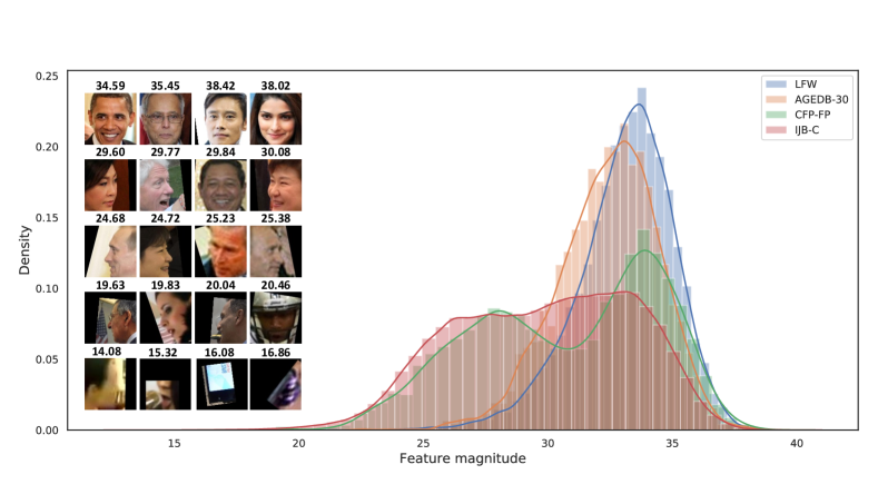
Figure 8: Extended Visualization of Figure 6.

B.2 Settings of $m(a_{i})$, $g(a_{i})$ and $\lambda_{g}$

In our experiments, we define function $m(a_{i})$ as a linear function defined on $[l_{a},u_{a}]$ with $m(l_{a})=l_{m},m(u_{a})=u_{m}$ and $g(a_{i})=\frac{1}{a_{i}}+\frac{1}{u_{a}^{2}}a_{i}$. Therefore, we have

Appendix C Ablation Study on Margin Distributions

In this section, effects of the feature distributions during training are studied. With $(\lambda_{g},l_{a},u_{a})$ fixed to $(35,10,110)$, we carefully select various combinations of $l_{m},u_{m}$ to align the mean margin on the training dataset to ArcFace (0.5) in our implementation. Features are distributed more separated if with a larger maximum margin and a smaller minimum margin.

Table 4 shows the recognition results with various hyper-parameters. With $(l_{m},u_{m})=(0.45,0.65)$, the penalty of magnitude loss degrades the performance of the recognition. With $(l_{m},u_{m})=(0.25,1.60)$, the performance is also worse than then baseline as hard samples are assigned to small margins (a.k.a., hard/noisy samples are down-weighted). Parameter $(0.40,0.80)$ balances the feature distribution and margins for hard/noisy samples, and therefore achieves a significant improvement on benchmarks.

Appendix D Extended Visualization of Figure 6

We present a extended visualization of figure 6 in figure 8 which has more examples of faces with feature magnitudes. All the faces are sample from the IJB-C benchmark. It can be seen that faces with magnitudes around 28 are mostly profile faces while around 35 are high-quality and frontal faces. That is consistent with the profile/frontal peaks in the CFP-FP benchmark and indicates that faces with similar magnitudes show similar quality patterns across benchmarks. In real applications, we can set a proper threshold for the magnitude and should be able to filter similar low-quality faces, even under various scenarios.

Besides directly served as qualities, our feature magnitudes can also be used as quality labels for faces, which avoids human labelling costs. These labels are more suitable for recognition, and therefore can be used to boost other quality models.

Appendix E Mag-CosFace

In the main text, MagFace is modified from the ArcFace loss. In this section, we show that MagFace based on CosFace loss (denote as Mag-CosFace) can theoretically achieve the same effects. Mag-CosFace loss for a sample $i$ is

Let $A(a_{i})=s(\cos\theta_{y_{i}}-m(a_{i}))$ and $B=\sum_{j=1,j\neq y_{i}}^{n}e^{s\cos{\theta_{j}}}$ and rewrite the loss as

E.1 Property of Convergence for Mag-CosFace

Property 5.

For $a_{i}\in[l_{a},u_{a}]$, $L_{i}$ is a strictly convex function of $a_{i}$.

Proof.

The first and second deriviates of $A(a_{i})$ are

$$A^{\prime}(a_{i}) =-sm^{\prime}(a_{i})$$ (12)

$$A^{\prime\prime}(a_{i}) =-sm^{\prime\prime}(a_{i})$$

As $A^{\prime\prime}(a_{i})\leq 0$, the property can be proved following that presented before.

∎

Property 6.

A unique optimal solution $a_{i}^{*}$ exists in $[l_{a},u_{a}]$.

Proof.

We only need to prove

Then it’s easy to have there is a unique optimu. ∎

E.2 Property of Monotonicity for Mag-CosFace

Property 7.

With fixed $f_{i}$ and $W_{j},j\in\{1,\cdots,n\},j\neq y_{i}$, the optimal feature magnitude $a^{*}_{i}$ is monotonically increasing if the cosine-distance to its class center $W_{y_{i}}$ decreases.

Proof.

The first derivate of $L_{i}$ is

For $\theta_{y_{i}}^{1}<\theta_{y_{i}}^{2}$, the core here is to prove $\frac{\partial L_{i}(\theta^{1}_{y_{i}})}{\partial a_{i}}<\frac{\partial L_{i}(\theta^{2}_{y_{i}})}{\partial a_{i}}$, which is obvious as $\cos\theta_{y_{i}}^{1}>\cos\theta_{y_{i}}^{2}$. The rest of the proofs is the same as those for the original MagFace. ∎

Property 8.

With other things fixed, the optimal feature magnitude $a^{*}_{i}$ is monotonically increasing with a decreasing $B$ (, increasing inter-class distance).

Proof.

It’s easy to have $\frac{\partial L_{i}(B_{1})}{\partial a_{i}}<\frac{\partial L_{i}(B_{2})}{\partial a_{i}}$ if $B_{1}<B_{2}$. The rest of the proofs is the same as those for the original MagFace. ∎

Appendix F Authors’ Contributions

Shichao Zhao and Zhida Huang contribute similarly to this work. Besides involved in discussions, Shichao Zhao mainly conducted experiments on face clustering and Zhida Huang implemented baselines as well as evaluation metrics for quality experiments.

References

- [1] Information technology – Biometric data interchange formats – Part 5: Face image data. Standard, International Or- ganization for Standardization, Nov. 2011.
- [2] Machine Readable Travel Documents. Standard, International Civil Aviation Organization, 2015.
- [3] Enrique Amigó, Julio Gonzalo, Javier Artiles, and Felisa Verdejo. A comparison of extrinsic clustering evaluation metrics based on formal constraints. Information retrieval, 12(4):461–486, 2009.
- [4] Lacey Best-Rowden and Anil K Jain. Learning face image quality from human assessments. IEEE Trans. Information Forensics and Security, 13(12):3064–3077, 2018.
- [5] Dong Cao, Xiangyu Zhu, Xingyu Huang, Jianzhu Guo, and Zhen Lei. Domain balancing: Face recognition on long-tailed domains. In IEEE Conference on Computer Vision and Pattern Recognition, pages 5671–5679, 2020.
- [6] Qiong Cao, Li Shen, Weidi Xie, Omkar M Parkhi, and Andrew Zisserman. VggFace2: A dataset for recognising faces across pose and age. In IEEE Int’l Conf. Automatic Face & Gesture Recognition (FG), pages 67–74. IEEE, 2018.
- [7] Jie Chang, Zhonghao Lan, Changmao Cheng, and Yichen Wei. Data uncertainty learning in face recognition. In IEEE Conference on Computer Vision and Pattern Recognition, pages 5710–5719, 2020.
- [8] Sumit Chopra, Raia Hadsell, and Yann LeCun. Learning a similarity metric discriminatively, with application to face verification. In IEEE Conference on Computer Vision and Pattern Recognition, volume 1, pages 539–546. IEEE, 2005.
- [9] Jiankang Deng, Jia Guo, Niannan Xue, and Stefanos Zafeiriou. ArcFace: Additive angular margin loss for deep face recognition. In IEEE Conference on Computer Vision and Pattern Recognition, pages 4690–4699, 2019.
- [10] Hang Du, Hailin Shi, Dan Zeng, and Tao Mei. The elements of end-to-end deep face recognition: A survey of recent advances. arXiv preprint arXiv:2009.13290, 2020.
- [11] Martin Ester, Hans-Peter Kriegel, Jörg Sander, Xiaowei Xu, et al. A density-based algorithm for discovering clusters in large spatial databases with noise. In KDD, volume 96, pages 226–231, 1996.
- [12] Patrick Grother and Elham Tabassi. Performance of biometric quality measures. IEEE Trans on Pattern Analysis and Machine Intelligence, 29(4):531–543, 2007.
- [13] Jianzhu Guo, Xiangyu Zhu, Chenxu Zhao, Dong Cao, Zhen Lei, and Stan Z Li. Learning meta face recognition in unseen domains. In IEEE Conference on Computer Vision and Pattern Recognition, pages 6163–6172, 2020.
- [14] Yandong Guo, Lei Zhang, Yuxiao Hu, Xiaodong He, and Jianfeng Gao. MS-Celeb-1M: A dataset and benchmark for large-scale face recognition. In European Conference on Computer Vision, pages 87–102. Springer, 2016.
- [15] Javier Hernandez-Ortega, Javier Galbally, Julian Fierrez, Rudolf Haraksim, and Laurent Beslay. FaceQnet: quality assessment for face recognition based on deep learning. In International Conference on Biometrics, 2019.
- [16] Gary B Huang, Marwan Mattar, Tamara Berg, and Eric Learned-Miller. Labeled faces in the wild: A database for studying face recognition in unconstrained environments. Technical Report 07-49, University of Massachusetts, Amherst, 2007.
- [17] Anil k. Jai, Richard C. Dubes, and Englewood Cliffs. Algorithms for clustering data. NJ:Prentice-Hall, 1988.
- [18] Bingyu Liu, Weihong Deng, Yaoyao Zhong, Mei Wang, Jiani Hu, Xunqiang Tao, and Yaohai Huang. Fair loss: margin-aware reinforcement learning for deep face recognition. In International Conference on Computer Vision, pages 10052–10061, 2019.
- [19] Hao Liu, Xiangyu Zhu, Zhen Lei, and Stan Z Li. AdaptiveFace: Adaptive margin and sampling for face recognition. In IEEE Conference on Computer Vision and Pattern Recognition, pages 11947–11956, 2019.
- [20] Weiyang Liu, Yandong Wen, Zhiding Yu, Ming Li, Bhiksha Raj, and Le Song. Sphereface: Deep hypersphere embedding for face recognition. In IEEE Conference on Computer Vision and Pattern Recognition, pages 212–220, 2017.
- [21] Stuart Lloyd. Least squares quantization in PCM. IEEE Trans. Information Theory, 28(2):129–137, 1982.
- [22] Brianna Maze, Jocelyn Adams, James A Duncan, Nathan Kalka, Tim Miller, Charles Otto, Anil K Jain, W Tyler Niggel, Janet Anderson, Jordan Cheney, et al. IARPA Janus benchmark-C: Face dataset and protocol. In International Conference on Biometrics, pages 158–165. IEEE, 2018.
- [23] Anish Mittal, Rajiv Soundararajan, and Alan C Bovik. Making a “completely blind” image quality analyzer. IEEE Signal processing letters, 20(3):209–212, 2012.
- [24] Stylianos Moschoglou, Athanasios Papaioannou, Christos Sagonas, Jiankang Deng, Irene Kotsia, and Stefanos Zafeiriou. AgeDB: the first manually collected, in-the-wild age database. In IEEE Conference on Computer Vision and Pattern Recognition Workshop, pages 51–59, 2017.
- [25] Rajeev Ranjan, Carlos D Castillo, and Rama Chellappa. L2-constrained softmax loss for discriminative face verification. arXiv preprint arXiv:1703.09507, 2017.
- [26] Torsten Schlett, Christian Rathgeb, Olaf Henniger, Javier Galbally, Julian Fierrez, and Christoph Busch. Face image quality assessment: A literature survey. arXiv preprint arXiv:2009.01103, 2020.
- [27] Florian Schroff, Dmitry Kalenichenko, and James Philbin. FaceNet: A unified embedding for face recognition and clustering. In IEEE Conference on Computer Vision and Pattern Recognition, pages 815–823, 2015.
- [28] Soumyadip Sengupta, Jun-Cheng Chen, Carlos Castillo, Vishal M Patel, Rama Chellappa, and David W Jacobs. Frontal to profile face verification in the wild. In IEEE Winter Conference on Applications of Computer Vision (WACV), pages 1–9. IEEE, 2016.
- [29] Yichun Shi and Anil K Jain. Probabilistic face embeddings. In International Conference on Computer Vision, pages 6902–6911, 2019.
- [30] Kihyuk Sohn. Improved deep metric learning with multi-class n-pair loss objective. In Annual Conference on Neural Information Processing Systems, pages 1857–1865, 2016.
- [31] Tao Sun, Xingjie Zhu, Jeng-Shyang Pan, Jiajun Wen, and Fanqiang Meng. No-reference image quality assessment in spatial domain. In Genetic and Evolutionary Computing, pages 381–388. Springer, 2015.
- [32] Yifan Sun, Changmao Cheng, Yuhan Zhang, Chi Zhang, Liang Zheng, Zhongdao Wang, and Yichen Wei. Circle loss: A unified perspective of pair similarity optimization. In IEEE Conference on Computer Vision and Pattern Recognition, pages 6398–6407, 2020.
- [33] Yi Sun, Ding Liang, Xiaogang Wang, and Xiaoou Tang. DeepID3: Face recognition with very deep neural networks. arXiv preprint arXiv:1502.00873, 2015.
- [34] Yi Sun, Xiaogang Wang, and Xiaoou Tang. Deep learning face representation from predicting 10,000 classes. In IEEE Conference on Computer Vision and Pattern Recognition, pages 1891–1898, 2014.
- [35] Yaniv Taigman, Ming Yang, Marc’Aurelio Ranzato, and Lior Wolf. DeepFace: Closing the gap to human-level performance in face verification. In IEEE Conference on Computer Vision and Pattern Recognition, pages 1701–1708, 2014.
- [36] Philipp Terhorst, Jan Niklas Kolf, Naser Damer, Florian Kirchbuchner, and Arjan Kuijper. SER-FIQ: Unsupervised estimation of face image quality based on stochastic embedding robustness. In IEEE Conference on Computer Vision and Pattern Recognition, 2020.
- [37] N Venkatanath, D Praneeth, Maruthi Chandrasekhar Bh, Sumohana S Channappayya, and Swarup S Medasani. Blind image quality evaluation using perception based features. In National Conference on Communications (NCC), pages 1–6. IEEE, 2015.
- [38] Feng Wang, Jian Cheng, Weiyang Liu, and Haijun Liu. Additive margin softmax for face verification. IEEE Signal Processing Letters, 25(7):926–930, 2018.
- [39] Feng Wang, Xiang Xiang, Jian Cheng, and Alan Loddon Yuille. NormFace: L2 hypersphere embedding for face verification. In ACM International Conference on Multimedia, pages 1041–1049, 2017.
- [40] Hao Wang, Yitong Wang, Zheng Zhou, Xing Ji, Dihong Gong, Jingchao Zhou, Zhifeng Li, and Wei Liu. CosFace: Large margin cosine loss for deep face recognition. In IEEE Conference on Computer Vision and Pattern Recognition, pages 5265–5274, 2018.
- [41] Jian Wang, Feng Zhou, Shilei Wen, Xiao Liu, and Yuanqing Lin. Deep metric learning with angular loss. In International Conference on Computer Vision, pages 2593–2601, 2017.
- [42] Xiaobo Wang, Shuo Wang, Shifeng Zhang, Tianyu Fu, Hailin Shi, and Tao Mei. Support vector guided softmax loss for face recognition. arXiv preprint arXiv:1812.11317, 2018.
- [43] Zhongdao Wang, Liang Zheng, Yali Li, and Shengjin Wang. Linkage based face clustering via graph convolution network. In IEEE Conference on Computer Vision and Pattern Recognition, 2019.
- [44] Yandong Wen, Kaipeng Zhang, Zhifeng Li, and Yu Qiao. A discriminative feature learning approach for deep face recognition. In European Conference on Computer Vision, pages 499–515. Springer, 2016.
- [45] Cameron Whitelam, Emma Taborsky, Austin Blanton, Brianna Maze, Jocelyn Adams, Tim Miller, Nathan Kalka, Anil K Jain, James A Duncan, Kristen Allen, et al. IARPA Janus benchmark-B face dataset. In IEEE Conference on Computer Vision and Pattern Recognition Workshop, pages 90–98, 2017.
- [46] Lei Yang, Dapeng Chen, Xiaohang Zhan, Rui Zhao, Chen Change Loy, and Dahua Lin. Learning to cluster faces via confidence and connectivity estimation. In IEEE Conference on Computer Vision and Pattern Recognition, 2020.
- [47] Dong Yi, Zhen Lei, Shengcai Liao, and Stan Z Li. Learning face representation from scratch. arXiv preprint arXiv:1411.7923, 2014.
- [48] Yuhui Yuan, Kuiyuan Yang, and Chao Zhang. Feature incay for representation regularization. arXiv preprint arXiv:1705.10284, 2017.
- [49] Xiao Zhang, Rui Zhao, Yu Qiao, Xiaogang Wang, and Hongsheng Li. AdaCos: Adaptively scaling cosine logits for effectively learning deep face representations. In IEEE Conference on Computer Vision and Pattern Recognition, pages 10823–10832, 2019.
- [50] Tianyue Zheng and Weihong Deng. Cross-pose LFW: A database for studying cross-pose face recognition in unconstrained environments. Beijing University of Posts and Telecommunications, Tech. Rep, 5, 2018.
- [51] Tianyue Zheng, Weihong Deng, and Jiani Hu. Cross-age LFW: A database for studying cross-age face recognition in unconstrained environments. arXiv preprint arXiv:1708.08197, 2017.