Towards Learning an Unbiased Classifier from Biased Data via Coditional Adversarial Debiasing

Abstract

Bias in classifiers is a severe issue of modern deep learning methods, especially for their application in safety- and security-critical areas. Often, the bias of a classifier is a direct consequence of a bias in the training dataset, frequently caused by the co-occurrence of relevant features and irrelevant ones. To mitigate this issue, we require learning algorithms that prevent the propagation of bias from the dataset into the classifier. We present a novel adversarial debiasing method, which addresses a feature that is spuriously connected to the labels of training images but statistically independent of the labels for test images. Thus, the automatic identification of relevant features during training is perturbed by irrelevant features. This is the case in a wide range of bias-related problems for many computer vision tasks, such as automatic skin cancer detection or driver assistance. We argue by a mathematical proof that our approach is superior to existing techniques for the abovementioned bias. Our experiments show that our approach performs better than state-of-the-art techniques on a well-known benchmark dataset with real-world images of cats and dogs.

1 Introduction

Deep neural networks have demonstrated impressive performances in many areas. These areas encompass not only classical computer vision tasks, like object detection or semantic segmentation, but also safety- and security-critical tasks, such as skin cancer detection [20] or predicting recidivism [4]. However, many people, including domain experts, advise against employing deep learning in those applications, even if these classifiers outperform human experts, for example, in skin lesion classification [28]. One reason for their concerns is bias in the classifiers. Indeed, almost all image datasets contain some kind of bias [30] and, consequently, the performance of classifiers varies significantly across subgroups. For example, the skin lesion classification performance varies across age groups [17], and recidivism prediction is biased against ethnic groups [4].

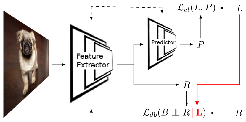
Figure 1: In adversarial debiasing, a debiasing loss $\mathcal{L}_{db}$ is often used to enforce independence between the bias variable $B$ and a representation $R$. In this work, we show that it is beneficial to condition this independence on the label $L$.

One major reason for bias in classifiers is dataset bias. Every dataset is a unique slice through the visual world [27]. Therefore, an image dataset often does not represent the real world perfectly but contains spurious dependencies between meaningless features and the labels of its samples. This spurious connection can be caused by incautious data collection or by justified concerns. If, for example, the acquirement of particular examples is dangerous, these examples might be left out of a dataset due to justified safety concerns. A classifier trained on such a dataset might pick the spuriously dependent feature to predict the label and is, thus, biased. In order to mitigate such a bias, it is important to understand the nature of the spurious dependence. Therefore, we start our investigation at the data generation process. We provide a formal description of the data generation model for a common computer vision bias in Section 3.1. In contrast to other approaches that do not provide a model for the data generation process and, hence, rely solely on empirical evaluations, this allows us to investigate our proposed method theoretically. We discuss the resulting differences to related work in Section 2. Additionally, our model provides a simple way for practitioners to determine whether our solution applies to a specific problem.

The main contribution of our work is a novel adversarial debiasing strategy. The basic concept of adversarial debiasing and the idea of our improvement can be observed in Figure 1. For adversarial debiasing, a second loss $\mathcal{L}_{db}$ is used in addition to the regular training loss $\mathcal{L}_{cl}$ of a neural network classifier. This second loss penalizes the dependence between the bias variable $B$ and an intermediate representation $R$ from the neural network. The main difference we propose in this paper is replacing this dependence $B\not\mathchoice{\mathrel{\hbox to0.0pt{$\displaystyle\perp$\hss}\mkern 2.0mu{\displaystyle\perp}}}{\mathrel{\hbox to0.0pt{$\textstyle\perp$\hss}\mkern 2.0mu{\textstyle\perp}}}{\mathrel{\hbox to0.0pt{$\scriptstyle\perp$\hss}\mkern 2.0mu{\scriptstyle\perp}}}{\mathrel{\hbox to0.0pt{$\scriptscriptstyle\perp$\hss}\mkern 2.0mu{\scriptscriptstyle\perp}}}R$ by the conditional dependence $B\not\mathchoice{\mathrel{\hbox to0.0pt{$\displaystyle\perp$\hss}\mkern 2.0mu{\displaystyle\perp}}}{\mathrel{\hbox to0.0pt{$\textstyle\perp$\hss}\mkern 2.0mu{\textstyle\perp}}}{\mathrel{\hbox to0.0pt{$\scriptstyle\perp$\hss}\mkern 2.0mu{\scriptstyle\perp}}}{\mathrel{\hbox to0.0pt{$\scriptscriptstyle\perp$\hss}\mkern 2.0mu{\scriptscriptstyle\perp}}}R\,|\,L$ with $L$ being the label. In fact, it turns out that this conditional dependence is better suited than the unconditional dependence for the considered kind of bias. The motivation for this replacement can be found in Section 3.2. Even more important, the formal description of the data generation model allows us to provide a rigorous mathematical proof for the linear case in Section 3.2, which can also be extended to the non-linear case. This proof demonstrates that our new approach fits the specific bias well.

To use our new conditional independence criterion for adversarial debiasing, we have to implement it as a differentiable loss. We provide three possible implementations in Section 3.3. To this end, we extend existing ideas from [21, 12, 15, 1] for implementing the unconditional independence criterion and provide realizations for their conditional counterparts. We demonstrate that these new loss functions lead to larger accuracies on unbiased test sets. In Section 4.1, we provide results of experiments on a synthetic dataset that maximizes the difference between the conditional and the unconditional dependence. Further, in Section 4.3, we present results on a dataset with real-world images of cats and dogs that is used by previous work to evaluate adversarial debiasing. These experiments show that our new approach outperforms existing methods on both synthetic and real-world data. Further experiments shown in Section 4.2 indicate that the proposed change of the criterion causes the increasing accuracies.

2 Related work

The goal of debiasing is to prevent a classifier from using biased features. To reach this goal, we first have to choose a criterion to determine whether the classifier uses a feature. Second, we have to turn this criterion into a differentiable loss. In this section, we compare our choices to related work from the literature.

First, we compare our criterion for determining whether the classifier uses a feature. Traditionally, adversarial debiasing aims to learn a feature representation that is informative for a task but independent of the bias. Hence, a second neural network that should predict the bias from the feature representation is introduced to enforce this independence. The original network for classification and this second network are then trained in an adversarial fashion. To this end, different loss functions for the original network are suggested to decrease the performance of the second network for predicting the bias. In [3], the authors minimize the cross-entropy between bias prediction and a uniform distribution. The mean squared error between the reconstruction and the bias is used in [32]. The authors of [12] maximize the cross-entropy between the predicted distribution of the bias and the bias variable. Additionally, they maximize the entropy of the distribution of the predicted bias. In [1], the authors minimize the correlation between the ground-truth bias and the prediction of the bias. However, as demonstrated in [23], independence is too restrictive as a criterion for determining whether a deep neural network uses a certain feature. This fact is also reflected in the experimental results of the abovementioned papers. The resulting classifiers are less biased, but this often leads to decreasing performance on unbiased test sets. For example, [3] report significantly less bias in an age classifier trained on a dataset biased by gender but the performance on the unbiased test set drops from $0.789$ to $0.781$. Our work is fundamentally different. Instead of a different loss, we suggest a different criterion to determine whether a neural network uses a feature. We use the conditional independence criterion proposed by [23] rather than independence between the representation and the bias.

To turn the chosen criterion, in our case, conditional independence, into a differentiable loss, we extend three ideas from the literature. We build on work of [21] and [15], which use the Hilbert-Schmidt independence criterion (HSIC) [8] as well as on the ideas of using mutual information presented in [12] or the predictability criterion presented by [1]. All three criteria are unconditional. Our work extends them to conditional independence criteria.

For understanding deep neural networks, [23] demonstrate that conditional dependence is a sharper criterion than unconditional dependence. For adversarial domain adaptation, [31] show significant improvements of conditional adversarial losses compared to unconditional adversarial losses. However, our work is the first one that makes use of these advantages in adversarial debiasing.

The authors of [24] use contextual decomposition [18] to force a neural network to focus on useful areas of an image. In contrast, we use the approach of [23], which can not only be applied to image areas but arbitrary features.

While the vast majority of adversarial debiasing methods acknowledge that bias has many forms, they rarely link the suggested solutions to the processes that generate the biased data. Instead, they rely exclusively on empirical evaluations. In contrast, we provide a specific model for a specific kind of bias as well as a theoretical proof that our approach is better suited for this case.

3 Proposed debiasing approach

In this section, we introduce and motivate our novel approach to adversarial debiasing. First, in Section 3.1, we define a model for the bias we consider in this work. Even though the bias model is quite specific, it covers many relevant cases in computer vision. We corroborate this claim with two examples at the end of Section 3.1. Afterward, we introduce our novel adversarial debiasing criterion. Section 3.2 provides a theoretical motivation and a mathematical proof that the new criterion fits our specific bias model better than existing solutions from the literature. Finally, we provide three possible implementations for loss functions that realize this criterion in Section 3.3.

3.1 Bias model

Figure 2: A graphical representation of the specific bias. Circles represent variables, dotted circles represent unobserved variables. The label $L$ is only dependent on a signal $S$, while the input $I$ is also dependent on some variable $B$. In the training set, the signal $S$ influences the variable $B$ due to bias. This is indicated by the red dashed arrow.

Many different kinds of bias exist and influence visual datasets in various ways [30]. In this work, we consider a specific kind of bias. We will later argue that this specific model covers many relevant tasks in computer vision.

To describe the bias model, we start with a graphical model of the underlying data generation process displayed in Figure 2. For classification tasks, like separating cats from dogs, we assume that a process following this graphical model generates the label $L$ (cat or dog) from a signal $S$. This signal $S$ is contained in and can be extracted from the input $I$. However, the input $I$ is a mixture of multiple signals: Besides $S$, another signal $B$ influences $I$. In the cat/dog example, $B$ might relate to the fur’s color. Since the fur’s color is not meaningful in distinguishing cats and dogs, $B$ is independent of $S$ and $L$ during the application of the machine learning method in practice, i.e., on an unbiased test set,

$$\textup{Test:}\quad B\mathchoice{\mathrel{\hbox to0.0pt{$\displaystyle\perp$\hss}\mkern 2.0mu{\displaystyle\perp}}}{\mathrel{\hbox to0.0pt{$\textstyle\perp$\hss}\mkern 2.0mu{\textstyle\perp}}}{\mathrel{\hbox to0.0pt{$\scriptstyle\perp$\hss}\mkern 2.0mu{\scriptstyle\perp}}}{\mathrel{\hbox to0.0pt{$\scriptscriptstyle\perp$\hss}\mkern 2.0mu{\scriptscriptstyle\perp}}}L.$$ (1)

In contrast, in a biased training set, we find an unwanted dependence between the signal $S$ and the signal $B$. Hence, we call $B$ the bias variable in this case. The training dataset in the cat/dog example might contain only images of dogs with bright fur and images of cats with dark fur, leading to

$$\textup{Training:}\quad B\not\mathchoice{\mathrel{\hbox to0.0pt{$\displaystyle\perp$\hss}\mkern 2.0mu{\displaystyle\perp}}}{\mathrel{\hbox to0.0pt{$\textstyle\perp$\hss}\mkern 2.0mu{\textstyle\perp}}}{\mathrel{\hbox to0.0pt{$\scriptstyle\perp$\hss}\mkern 2.0mu{\scriptstyle\perp}}}{\mathrel{\hbox to0.0pt{$\scriptscriptstyle\perp$\hss}\mkern 2.0mu{\scriptscriptstyle\perp}}}L.$$ (2)

This dependence can be utilized by a machine-learning algorithm to predict $L$ using $B$, resulting in a biased classifier.

To better understand the direction of the arrow from $S$ to $B$, we want to emphasize, that data for a task is selected with a purpose. Images are included in the dataset because they show cats or dogs and one will, if necessary, deliberately accept imbalances in variables like fur-color. In contrast, if one find that our dataset misrepresents fur-color one would never accept a major misrepresentation of the ratio of cats and dogs to compensate for this problem. This demonstrates, that $S$ influences $B$ through the dataset creation while $B$ does not influence $S$.

This bias model covers many relevant situations in computer vision. In the following, we give two examples where the bias model fits the data and one where it does not.

The first example is a driver assistance system that uses a camera to estimate aquaplaning risk [10]. To train such a system, a dataset is needed that contains images of safe conditions and aquaplaning conditions. While the images of safe conditions can be easily collected in the wild, it is dangerous to drive a car under aquaplaning conditions. Therefore, the images of aquaplaning conditions must be collected in a specific facility. In this example, the signal $S$ is the standing water, and the bias variable $B$ is the location that determines the background of the image. Because of this safety risk, they are dependent in the training set, but not at the time of application.

The second example is automatic classification of skin lesions from images [29]. The classification systems are trained on images taken by dermatologists. Since the growth of the skin lesion is informative for skin lesion classification, dermatologists sometimes draw a scale next to the skin lesion if they suspect it is malignant. In this example, the characteristics of the skin lesion form the signal $S$, while the drawn scale is the bias variable $B$. These are dependent in the training set, but this bias is not present in the application.

The third example is the one, where the bias model does not fit the data. The example is a system that predicts absenteeism in the workplace, for example [2]. If an automated system predicts absenteeism, it might be unfair to women because of pregnancy. And we might want a system that does not take this effect into account. Here, the bias variable $B$ is the sex and the signal $S$ is the time an employee will be absent from work. Here, our bias model does not fit because the data contain a $B$ to $L$ link.

3.2 Conditional independence for debiasing

Deep neural networks unite a feature extractor and a predictor [22]. For adversarial debiasing, we separate the two at some intermediate layer. We denote the output of the feature extractor $R$. Note that it is a valid approach to use the whole network for feature extraction. In this case, $R$ is the prediction of the neural network. Both networks are trained using a classification loss $\mathcal{L}_{cl}$, e.g., cross-entropy loss. Additionally, a debiasing loss $\mathcal{L}_{db}$ is used to prevent the extraction of the bias variable $B$. For a visualization, see Figure 1. Most approaches for adversarial debiasing [3, 32, 1, 12] aim to find a representation $R$ of $I$ that is independent of the bias variable $B$ while still being informative for the label $L$, i.e.,

$$R\mathchoice{\mathrel{\hbox to0.0pt{$\displaystyle\perp$\hss}\mkern 2.0mu{\displaystyle\perp}}}{\mathrel{\hbox to0.0pt{$\textstyle\perp$\hss}\mkern 2.0mu{\textstyle\perp}}}{\mathrel{\hbox to0.0pt{$\scriptstyle\perp$\hss}\mkern 2.0mu{\scriptstyle\perp}}}{\mathrel{\hbox to0.0pt{$\scriptscriptstyle\perp$\hss}\mkern 2.0mu{\scriptscriptstyle\perp}}}B\quad\land\quad R\not\mathchoice{\mathrel{\hbox to0.0pt{$\displaystyle\perp$\hss}\mkern 2.0mu{\displaystyle\perp}}}{\mathrel{\hbox to0.0pt{$\textstyle\perp$\hss}\mkern 2.0mu{\textstyle\perp}}}{\mathrel{\hbox to0.0pt{$\scriptstyle\perp$\hss}\mkern 2.0mu{\scriptstyle\perp}}}{\mathrel{\hbox to0.0pt{$\scriptscriptstyle\perp$\hss}\mkern 2.0mu{\scriptscriptstyle\perp}}}L.$$ (3)

In this work, we propose a novel strategy: Instead of independence, we aim for conditional independence of $R$ and $B$, given the label $L$, i.e.,

$$R\mathchoice{\mathrel{\hbox to0.0pt{$\displaystyle\perp$\hss}\mkern 2.0mu{\displaystyle\perp}}}{\mathrel{\hbox to0.0pt{$\textstyle\perp$\hss}\mkern 2.0mu{\textstyle\perp}}}{\mathrel{\hbox to0.0pt{$\scriptstyle\perp$\hss}\mkern 2.0mu{\scriptstyle\perp}}}{\mathrel{\hbox to0.0pt{$\scriptscriptstyle\perp$\hss}\mkern 2.0mu{\scriptscriptstyle\perp}}}B\,|\,L\quad\land\quad R\not\mathchoice{\mathrel{\hbox to0.0pt{$\displaystyle\perp$\hss}\mkern 2.0mu{\displaystyle\perp}}}{\mathrel{\hbox to0.0pt{$\textstyle\perp$\hss}\mkern 2.0mu{\textstyle\perp}}}{\mathrel{\hbox to0.0pt{$\scriptstyle\perp$\hss}\mkern 2.0mu{\scriptstyle\perp}}}{\mathrel{\hbox to0.0pt{$\scriptscriptstyle\perp$\hss}\mkern 2.0mu{\scriptscriptstyle\perp}}}L.$$ (4)

Our strategy is better suited for the specific bias model presented in Section 3.1. In this section, we show that our strategy agrees with state-of-the-art results in explaining deep neural networks [23]. An optimal classifier fulfills the conditional independence (4) but not the independence (3). We prove this statement for the case that all data generation processes are linear. Consequently, loss functions that enforce the independence (3) will decrease the classifier’s performance, while loss functions that ensure the conditional independence (4) will not.

The goal of debiasing is to prevent a deep neural network from using a biased feature. To reach this goal, we first need to determine whether a classifier uses a feature. So far, most approaches for adversarial debiasing use the dependence between a feature and the classifier’s prediction to measure whether a classifier is using a feature. In contrast, we build on previous work for understanding deep neural networks [23]. While the independence criterion (3) obviously ensures that a bias variable $B$ is not used for classification, the authors of [23] reveal that independence is too restrictive to determine whether a deep neural network uses a certain feature. They employ the framework of causal inference [19] to show that the ground-truth labels are a confounding variable for features of the input and the predictions of a deep neural network. In theoretical considerations and empirical experiments, they further demonstrate that the prediction of a neural network and a feature of the input can be dependent even though the feature is not used by the deep neural network. The authors, therefore, suggest using the conditional independence (4), which we employ in our method for adversarial debiasing.

Thus, the independence criterion (3) is too strict. Even if the deep neural network ignores the bias, it might not satisfy (3) and, hence, not minimize a corresponding loss. Furthermore, minimizing such a loss based on the independence criterion will likely result in a less accurate classifier. To corroborate this claim, we present a mathematical proof for the following statement. If the bias can be modeled as explained in Section 3.1, the optimal classifier, which recovers the signal and calculates the correct label for every input image, fulfills the conditional independence (4) but not the independence (3). In this work, we only include the proof for the linear case, i.e., all data generating processes are linear. However, this proof can further be extended to the non-linear case by using a kernel space in which the data generation processes are linear and replacing covariances with the inner product of that space.

Theorem 1.

If the bias can be modeled as described in Section 3.1, the optimal classifier fulfills the conditional independence in (4) but not the independence in (3).

Proof.

Throughout this proof, we denote all variables with capital Latin letters. Capital Greek letters denote processes. For these processes, we denote the linear coefficients with lower-case Greek letters. The only exception to this is the optimal classifier that is denoted by $F^{\ast}$.

We start the proof by defining all functions involved in the model. Afterward, since dependence results in correlation in the linear case, a simple calculation proves the claim. Let $S$ denote the signal according to the bias model, as explained in Section 3.1. Since we are in the linear case, the bias variable $B$ can be split into a part that is fully determined by $S$ and a part that is independent of $S$.

Let $B^{\ast}$ be the part of the bias variable that is independent of $S$. The bias variable $B$ is given by

$$B=\alpha_{1}S+\alpha_{2}B^{\ast}=:\Phi\left(S,B^{\ast}\right).$$ (5)

Further, the label $L$ can be calculated from the signal $S$

$$L=\zeta_{1}S=:\Xi\left(S\right)$$ (6)

and the image $I$ is given by

$$I=:\Psi\left(S,B\right)=\Psi\left(S,\Phi\left(S,B^{\ast}\right)\right).$$ (7)

The optimal solution $F^{\ast}$ of the machine learning problem will recover the signal and calculate the label. By the assumptions of the bias model, the signal can be recovered from the input. Thus, there exists a function $\Psi^{\dagger}$ such that

$$\Psi^{\dagger}\left(\Psi\left(S,B\right)\right)=S$$ (8)

holds. Therefore, $F^{\ast}$ is given by

$$F^{\ast}:=\Xi\Psi^{\dagger}.$$ (9)

Now, we have defined all functions appearing in the model. The rest of the proof are two straightforward calculations. In the linear case, the independence of variables is equivalent to variables being uncorrelated. We denote the covariance of two variables $A,B$ with $\langle A,B\rangle$. To prove that (3) does not hold, we calculate

$$\begin{split}\left\langle F^{\ast}(I),B\right\rangle&=\left\langle\Xi\Psi^{\dagger}\Psi\left(S,\Phi\left(S,B^{\ast}\right)\right),\Phi\left(S,B^{\ast}\right)\right\rangle\\ &=\left\langle\zeta_{1}S,\alpha_{1}S+\alpha_{2}B^{\ast}\right\rangle=\zeta_{1}\alpha_{1}\left\langle S,S\right\rangle.\end{split}$$ (10)

This is equal to zero if and only if either all inputs contain an identical signal ($\left\langle S,S\right\rangle=0$), the dataset is unbiased ($\alpha_{1}=0$), or the label does not depend on the signal ($\zeta_{1}=0$).

For conditional independence, we can use partial correlation and obtain that $\left\langle F^{\ast}(I),B\right\rangle|L$ equals

$$\left\langle F^{\ast}(I)-\frac{\left\langle F^{\ast}(I),L\right\rangle}{\left\langle L,L\right\rangle}L,B-\frac{\left\langle B,L\right\rangle}{\left\langle L,L\right\rangle}L\right\rangle.$$ (11)

We substitute $L$ by (6) and use the properties of the inner product to arrive at

$$\begin{split}&\left\langle F^{\ast}(I),B\right\rangle-\frac{\left\langle\zeta_{1}S,\zeta_{1}S\right\rangle\left\langle\zeta_{1}S,B\right\rangle}{\left\langle\zeta_{1}S,\zeta_{1}S\right\rangle}\\ &=\zeta_{1}\alpha_{1}\left\langle S,S\right\rangle-\frac{\alpha_{1}\zeta_{1}^{3}\left\langle S,S\right\rangle^{2}}{\zeta_{1}^{2}\left\langle S,S\right\rangle}=0.\end{split}$$ (12)

This completes the proof for the linear case. For more detailed calculations see Section A in the Appendix. ∎

The optimal classifier does not minimize loss criteria based on the independence (3). Further, from (10), we see that the dependence contains $\zeta_{1}$, which is the correlation between the signal $S$ and the neural network’s prediction. Loss functions based on that criterion aim to reduce this parameter and, hence, will negatively affect the classifier’s performance. We demonstrate this effect using a synthetic dataset in Section 4. In contrast, loss terms based on our new criterion (4) are minimized by the optimal classifier. Thus, corresponding loss functions do not reduce the accuracy to minimize bias.

3.3 Implementation details

In Section 3.2, we presented two reasons that indicate why our new criterion (4) is better suited than the old criterion (3) for the bias described in Section 3.1. In practice, we are faced with the problem of integrating our criterion into the end-to-end learning framework of deep neural networks. As a consequence, we provide three possibilities to realize (4) as a loss function.

Turning an independence criterion into a loss function is not straightforward. First, the result of an independence test is binary and, hence, non-differentiable. Second, we need to consider distributions of variables to perform an independence test. However, we only see one mini-batch at a time during the training of a deep neural network. Nevertheless, multiple solutions exist in the unconditional case. In this section, we describe three possible solutions, namely: mutual information (MI), the Hilbert-Schmidt independence criterion (HSIC) and the maximum correlation criterion (MCC). We adapt the corresponding solutions from the unconditional case and extend them to conditional independence criteria.

The first solution makes use of the mutual information of $R$ and $B$ as suggested in [12],

$$\textup{MI}(R;B)=\sum_{r\in\mathcal{R},b\in\mathcal{B}}p_{R,B}(r,b)\log\frac{p_{R,B}(r,b)}{p_{R}(r)p_{B}(b)}.$$ (13)

Here, the criterion for independence is $\textup{MI}(R;B)=0$, and the mutual information is the differentiable loss function. However, to evaluate this loss, we must estimate the densities $p_{R,B},p_{R}$ and $p_{B}$ in every step, which is difficult. To mitigate this issue, the authors of [12] make simplifications to find a bound that is tractable for single examples. In contrast, we use conditional independence. Our criterion is $\textup{MI}(R;B|L)=0$, and the loss is given by the conditional mutual information $\textup{MI}(R;B|L)$

$$\sum_{\begin{subarray}{c}l\in\mathcal{L},b\in\mathcal{B}\\ r\in\mathcal{R}\end{subarray}}p_{R,B,L}\left(r,b,l\right)\log\frac{p_{L}(l)p_{R,B,L}\left(r,b,l\right)}{p_{R,L}(r,l)p_{B,L)}}.$$ (14)

We use kernel density estimation on the mini-batches to determine the densities and employ a Gaussian kernel with a variance of one-fourth of the average pairwise distance within a mini-batch. This setting proved best in preliminary experiments on reconstructing densities.

As a second solution, we extend the Hilbert Schmidt independence criterion [8]

$$\textup{HSIC}(R,B)=\frac{1}{(m-1)^{2}}\textup{tr}\,K_{R}HK_{B}H.$$ (15)

Here, $K_{R}$ and $K_{B}$ denote the kernel matrices for $R$ and $B$, respectively. For the Kronecker-Delta $\delta_{ij}$ and $m$ the number of examples, $H$ is given by $H_{ij}=\delta_{ij}-m^{-2}$. The variables are independent if and only if $\textup{HSIC}(R,B)=0$ holds for a sufficiently large kernel space. The HSIC was suggested for classical machine learning methods by [21] and [15]. Since we aim for conditional independence rather than independence, we use the conditional independence criterion [7]

$$\textup{tr}\,G_{R}S_{L}G_{B}S_{L}=0.$$ (16)

Here, for $X\in\{B,R,L\}$, we use $G_{X}=HK_{X}H$ and $S_{L}=\left(\mathbb{I}+1/mG_{L}\right)^{-1}$ with the identity matrix $\mathbb{I}$. For the relation to HSIC and further explanations, we refer to [7]. We use the same kernel as above and estimate the loss on every mini-batch independently.

The third idea we extend is the predictability criterion from [1]

$$\max_{f}\quad\textup{Corr}(f(R),B)=0.$$ (17)

To use this criterion within a loss function, they parametrize $f$ by a neural network. However, this is not an independence criterion as it can be equal to zero, even if $R$ and $B$ are dependent. Therefore, it is unclear how to incorporate the conditioning on $L$. As a consequence, we decided to extend the proposed criterion in two ways. First, we use the maximum correlation coefficient (MCC)

$$\textup{MCC}(R,B)=\max_{f,g}\quad\textup{Corr}(f(R),g(B))=0\quad,$$ (18)

which is equal to zero if and only if the two variables are independent [25]. Second, we use the partial correlation conditioned on the label $L$, which leads to

$$\max_{f,g}\quad\textup{PC}(f(R),g(B)\,|\,L)=0.$$ (19)

To parameterize both functions $f$ and $g$, we use neural networks. The individual effects of the two extensions can be observed through our ablation study in Section 4.2.

Note that all three of these implementations can be used for vector-valued variables. Therefore, they can also be used for multiple bias variables in parallel.

4 Experiments and results

This section contains empirical results that confirm our theoretical claims and form the third reason for the suitability of our proposed method. To this end, we first present experiments on a synthetic dataset that is designed to maximize the difference between the independence criterion (3) and the conditional independence criterion (4). Afterward, we report the results of an ablation study demonstrating that the gain in performance can be credited to the change of the independence criterion. Finally, we show that our findings also apply to a real-world dataset. For this purpose, we present experiments on different biased subsets of the cats and dogs dataset presented in [14].

To evaluate our experiments, we measure the accuracy on an unbiased testset. We do this for multiple reasons. First, we designed this method for situations in which a dataset is biased, but we expect the system to be used in an unbiased, real-world situation. Hence, the accuracy on an unbiased testset is our goal and evaluating it directly is the most precise measure for our method. Nevertheless, our method is also applicable to some situations of algorithmic fairness where we do not have access to an unbiased testset. In these situations it is common to use other evaluation methods like the “equalized odds” [9]

$$R\mathchoice{\mathrel{\hbox to0.0pt{$\displaystyle\perp$\hss}\mkern 2.0mu{\displaystyle\perp}}}{\mathrel{\hbox to0.0pt{$\textstyle\perp$\hss}\mkern 2.0mu{\textstyle\perp}}}{\mathrel{\hbox to0.0pt{$\scriptstyle\perp$\hss}\mkern 2.0mu{\scriptstyle\perp}}}{\mathrel{\hbox to0.0pt{$\scriptscriptstyle\perp$\hss}\mkern 2.0mu{\scriptscriptstyle\perp}}}B\,|\,L$$ (20)

or “demographic parity” [6]

$$R\mathchoice{\mathrel{\hbox to0.0pt{$\displaystyle\perp$\hss}\mkern 2.0mu{\displaystyle\perp}}}{\mathrel{\hbox to0.0pt{$\textstyle\perp$\hss}\mkern 2.0mu{\textstyle\perp}}}{\mathrel{\hbox to0.0pt{$\scriptstyle\perp$\hss}\mkern 2.0mu{\scriptstyle\perp}}}{\mathrel{\hbox to0.0pt{$\scriptscriptstyle\perp$\hss}\mkern 2.0mu{\scriptscriptstyle\perp}}}B$$ (21)

both of which are the same in this situation, since the testset is unbiased. The main drawback of these measures is that they are binary and, therefore, rather coarse-grained. Hence, we focus on the accuracy on unbiased testsets in this paper, but include the evaluations of these fairness criteria in Section B of the appendix.

4.1 Synthetic data

If a feature is independent of the label for a given classification task, the independence criterion (3) and the conditional independence criterion (4) agree. Since we aim to maximize the difference between the two criteria, we use a dataset with a strong dependence between the label $L$ and the variable $B$. We create a dataset of eight-by-eight pixels images that combine two signals. The first signal $S$, determines the shape of high-intensity pixels in the image. This shape is either a cross or a square, both consisting of the same number of pixels. The second signal $B$ is the color of the image. The hue of all pixels is either set to 0.3 (green) or to 0.9 (violet). Afterward, we add noise to the hue and the intensity value of every pixel. The noise is sampled from a uniform distribution on the interval $[-0.1,0.1]$. Finally, the images are converted to the RGB colorspace. To maximize the dependence between the label $L$ and the bias variable $B$, every training image of a cross is green and every training image of a square is violet. In the test set, these two signals are independent. Example images from the training and test set can be seen in Figure 3. We decided to limit the training set to 600 images for two reasons. First, small datasets are the expected use-case for adversarial debiasing. Second, this limitation increases the difficulty of debiasing.

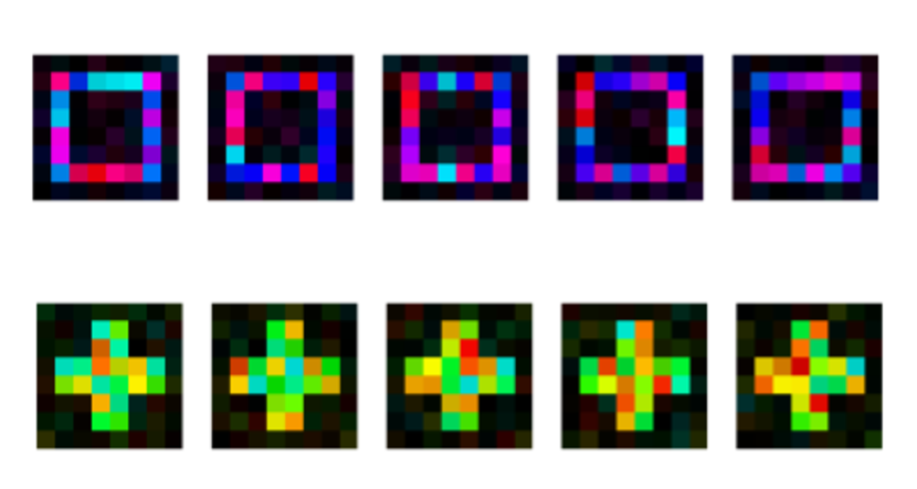
(a) Images from the training set

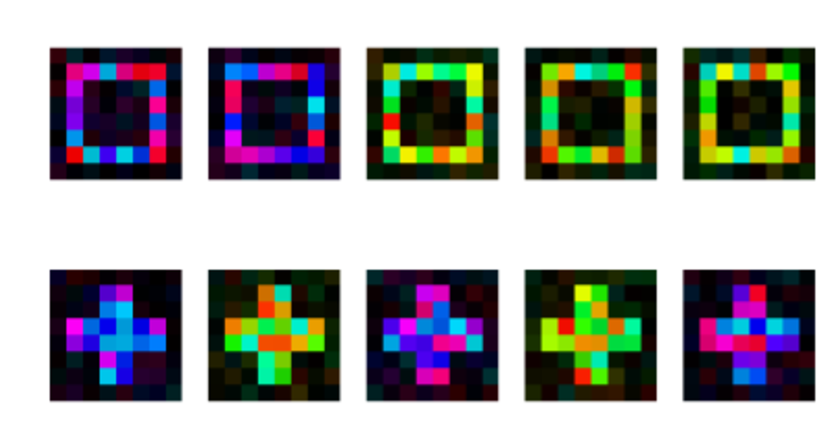
(b) Images from the test set

Figure 3: Example images from the synthetic dataset. In the training set, the color and the shape are dependent. In the test set, the two signals are independent.

For our first experiment, we use the shape as a categorical label $L$ and the color as the bias variable $B$. For this purpose, we calculate the mean color of the image after the noise is applied and use this value as the variable $B$. We report the results of this experiment in Table 1 in the column titled Setup I. To avoid any influence of shape- or color-preference, we also report results for the inverse setting in a second experiment, denoted as Setup II. For this experiment, we use the color as a categorical label $L$. The bias variable $B$ is then calculated as the difference between the values of pixels in the square shape and those in the cross.

As the backbone, we use a neural network that first contains two convolutional layers, each having 16 filter kernels of size $3{\times}3$. Then, a dense layer follows with 128 hidden neurons. These layers use ReLU activations. Finally, we use a dense layer with two neurons and softmax activation for classification. If a method from the literature uses an intermediate representation, we use the representation after the last convolutional layer. Otherwise, we use the prediction of the whole network as the representation $R$. Whenever an additional neural network is required by a method, i.e., all literature methods and ours based on MCC, we use a neural network with one hidden layer of 1024 neurons. For optimization, we use Adam [13].

As a baseline, we use the backbone neural network without any debiasing method. We have reimplemented four methods from the literature using the descriptions in the respective papers. The corresponding references can be found in Table 1. Two methods are proposed in [32]. We call the first, which penalizes the predictability of $B$ from $R$, Zhang et al. I. The second one, which penalizes predictability of $B$ from $R$ and $L$, is called Zhang et al. II. In addition, we report the averaged accuracies for these and all three implementations of our proposed criterion in Table 1.

We have set the hyperparameters for the competing methods to the values found in the corresponding papers. For all unpublished or problem-specific hyperparameters such as learning rates, as well as for all hyperparameters for our implementation, we used a grid search. To this end, we trained ten neural networks for each combination of different hyperparameters and evaluated them on an unbiased validation set. We included the list of the hyperparameters for every method in Section C in the appendix. For the second setup, we applied the same hyperparameter search. This resulted in different hyperparameters compared to the first setup for all methods, which are also described in Section C in the appendix.

Table 1: The results from 100 runs of our method and all baseline methods. For both experiments, we report the mean accuracy $\pm$ standard error. Best results are marked in bold

Method	Setup I	Setup II
Baseline	$0.819$ $\pm 0.016$	$0.791$ $\pm 0.016$
Adeli et al. [1]	$0.747$ $\pm 0.015$	$0.776$ $\pm 0.014$
Zhang et al. I [32]	$0.736$ $\pm 0.018$	$0.837$ $\pm 0.017$
Zhang et al. II [32]	$0.747$ $\pm 0.016$	$0.750$ $\pm 0.013$
Kim et al. [12]	$0.771$ $\pm 0.012$	$0.767$ $\pm 0.016$
Ours(MI)	$0.840$ $\pm 0.014$	0.871 $\pm 0.012$
Ours(HSIC)	$0.846$ $\pm 0.021$	$0.868$ $\pm 0.013$
Ours(MCC)	0.854 $\pm 0.013$	$0.867$ $\pm 0.013$

We observe that the baseline reaches a test accuracy of more than 75% in both experiments. Hence, hyperparameter selection influences which feature (color or shape) the neural network uses for classifications. Since there is no analytical way to determine the best hyperparameters, this strong impact might obscure the effect of debiasing methods. We tried to prevent this by rigorous hyperparameter optimization and a large number of runs.

We see that the difference between the methods from the literature using the independence criterion (3) and the methods using our new conditional independence criterion (4) is much larger than the differences between methods within these groups. For the first experiment, the worst method using (4) performs $5.9$ percentage points better than the best method using (3). The difference between the best and worst methods within these groups is $1.4$ percentage points and $3.5$ percentage points, respectively. In the second setup, the results are similar. Only the method suggested in [32] performs surprisingly good in this experiment.

We draw two conclusions from these experiments. First, as intended, the synthetic dataset is challenging for all existing methods found in the literature. In the first setup, none of them were able to improve the results of the baseline. In the second experiment, only one method outperformed the baseline. This coincides with observations from the literature that adversarial debiasing methods are challenged in situations with strong bias and lose accuracy to reduce bias. It also agrees with (10), which we discussed at the end of Section 3.2. It is important to note that we were able to reach the baseline performance for every method by allowing hyperparameters that deactivate the debiasing, e.g., by setting the weight of the debiasing loss to zero. To avoid this deactivation, we have limited the hyperparameters to the range that is used in the respective publications. Second, we observe that all methods that use our new debiasing criterion (4) reach a higher test accuracy than the baseline and, consequently, also a higher accuracy than existing methods.

4.2 Ablation study

In the previous experiment, we observed that our new methods reached a higher accuracy than the methods from the literature. To show that this increase in accuracy can be attributed to the conditional independence criterion (4), we conduct an ablation study for the three methods described in Section 3.3. More specifically, we first report results for a method using unconditional mutual information, calculated in the same way we calculate the conditional mutual information. Second, we present results for a method using the unconditional HSIC as a loss. Third, we present two methods that investigate the gap between the method presented by Adeli et al. [1] and our method using the conditional maximal correlation coefficient. The first one uses the unconditional maximum correlation coefficient, and the second one incorporates the partial correlation (PC) instead of the correlation in (17). We use the settings and evaluation protocol of Setup I and Setup II from the previous section. The results are presented in Table 2.

Table 2: The results of the ablation study. Every method is trained on a biased training set and evaluated on an unbiased test set. We report the accuracy averaged over 100 runs and the standard error. Best results are marked in bold

Method	Setup I	Setup II
Unconditional MI	$0.583$ $\pm 0.010$	$0.833$$\pm 0.011$
Conditional MI	0.840 $\pm 0.014$	0.871$\pm 0.012$
Unconditional HSIC	$0.744$ $\pm 0.011$	$0.590$$\pm 0.011$
Conditional HSIC	0.846 $\pm 0.021$	0.868$\pm 0.013$
Adeli et al. [1]	$0.747$ $\pm 0.015$	$0.776$$\pm 0.014$
Ours(MCC) – only MCC	$0.757$ $\pm 0.016$	$0.807$$\pm 0.015$
Ours(MCC) – only PC	$0.836$ $\pm 0.014$	$0.830$$\pm 0.015$
Ours(MCC) – complete	0.854 $\pm 0.013$	0.867$\pm 0.013$

We find that the unconditional versions of our methods, especially for mutual information (“Unconditional MI”) and HSIC (“Unconditional HSIC”), perform worse than almost all methods from the literature (see Setup I in Table 1). For the third method, we observe that the change from the predictability criterion to the maximum correlation coefficient increases the accuracy by 1.0 and 1.8 percentage points for the correlation and partial correlation case, respectively. In contrast, the change from correlation to partial correlation increases the accuracy by 8.9 percentage points with the predictability criterion and by 9.7 percentage points with the maximum correlation coefficient. These observations indicate that the improvements that we found in Section 4.1 can be attributed to the difference between (3) and (4) and not to implementation details.

4.3 Real-world data

Table 3: Experimental results on the cats and dogs dataset. All methods were trained on a dataset in which p% of all dogs are dark-furred dogs and $p$% of all cats are light-furred. The first column of the table indicates the fraction $p$. The following columns contain the accuracies on an unbiased test set averaged over three runs. We also report the standard error

Fraction	Baseline	Adeli et al. [1]	Zhang et al. I [32]	Zhang et al. II [32]	Ours(HSIC)
0%	0.627 $\pm 0.004$	0.597 $\pm 0.004$	0.590 $\pm 0.002$	0.617 $\pm 0.001$	0.615 $\pm 0.005$
10%	0.800 $\pm 0.001$	0.774 $\pm 0.002$	0.779 $\pm 0.005$	0.785 $\pm 0.007$	0.801 $\pm 0.001$
20%	0.845 $\pm 0.003$	0.829 $\pm 0.000$	0.812 $\pm 0.002$	0.809 $\pm 0.005$	0.855 $\pm 0.004$
30%	0.852 $\pm 0.007$	0.842 $\pm 0.003$	0.837 $\pm 0.004$	0.834 $\pm 0.003$	0.863 $\pm 0.002$
40%	0.859 $\pm 0.007$	0.855 $\pm 0.004$	0.870 $\pm 0.002$	0.850 $\pm 0.001$	0.875 $\pm 0.003$
50%	0.859 $\pm 0.006$	0.866 $\pm 0.003$	0.856 $\pm 0.001$	0.853 $\pm 0.001$	0.860 $\pm 0.002$
60%	0.866 $\pm 0.006$	0.837 $\pm 0.001$	0.850 $\pm 0.003$	0.860 $\pm 0.004$	0.856 $\pm 0.005$
70%	0.844 $\pm 0.003$	0.854 $\pm 0.003$	0.835 $\pm 0.005$	0.841 $\pm 0.005$	0.859 $\pm 0.000$
80%	0.829 $\pm 0.002$	0.822 $\pm 0.005$	0.820 $\pm 0.005$	0.826 $\pm 0.003$	0.836 $\pm 0.002$
90%	0.773 $\pm 0.010$	0.743 $\pm 0.001$	0.758 $\pm 0.001$	0.731 $\pm 0.002$	0.791 $\pm 0.004$
100%	0.612 $\pm 0.001$	0.612 $\pm 0.004$	0.604 $\pm 0.001$	0.609 $\pm 0.001$	0.616 $\pm 0.002$

Table 4: The results of the ablation study on the real data. Our conditional HSIC and an unconditional HSIC methods were trained on a dataset in which p% of all dogs are dark-furred dogs and $p$% of all cats are light-furred. The first column of the table indicates the fraction $p$. The following columns contain the accuracies on an unbiased test set averaged over three runs. We also report the standard error

	Unconditional
Fraction	HSIC	HSIC (Ours)	Diff
0%	$0.611$$\pm 0.003$	0.615$\pm 0.005$	0.004
10%	$0.759$$\pm 0.012$	0.801$\pm 0.001$	0.042
20%	$0.816$$\pm 0.002$	0.855$\pm 0.004$	0.039
30%	$0.834$$\pm 0.002$	0.863$\pm 0.002$	0.029
40%	$0.861$$\pm 0.003$	0.875$\pm 0.003$	0.014
50%	$0.863$$\pm 0.004$	0.860$\pm 0.002$	-0.003
60%	$0.844$$\pm 0.001$	0.856$\pm 0.005$	0.012
70%	$0.835$$\pm 0.003$	0.859$\pm 0.000$	0.024
80%	$0.820$$\pm 0.007$	0.836$\pm 0.002$	0.016
90%	$0.757$$\pm 0.003$	0.791$\pm 0.004$	0.034
100%	$0.606$$\pm 0.002$	0.616$\pm 0.002$	0.010

After we have demonstrated the effectiveness of our approach on a synthetic dataset, we conduct a third experiment to investigate whether the increase in accuracy can be observed in real-world image data as well. Even though the described bias is present in many computer vision tasks, most datasets are inadequate for our investigations. To evaluate the performance of our debiasing method, we require an unbiased test set. However, most datasets contain the same bias in their training and test sets since both sets are collected in the same way. To mitigate this problem, we consider a dataset, which has labels for multiple signals per image. This allows us to introduce a bias in the training set but not in the test set. To this end, we use the cats and dogs dataset that was used for the same purpose in [14].

This dataset contains images of cats and dogs that are additionally labeled as dark-furred or light-furred. We first remove 20% of each class/fur combination as an unbiased test set. Then, we create eleven training sets with different levels of bias. We start with a training set that contains only light-furred dogs and only dark-furred cats. For each of the other sets, we increase the fraction of dark-furred dogs and light-furred cats by ten percent. Therefore, the last dataset contains only dark-furred dogs and light-furred cats. We equalize the size of all these training sets to perform a fair evaluation. Unfortunately, this limits the training set size to 80% of the rarest class/fur combination. Therefore, the training sets contain only $2{,}469$ images, which is $14.7\%$ of the original training set.

As a backbone network, we use a ResNet-18 [11]. We train the network for 150 epochs using the Adam optimizer [13]. The learning rate follows a cosine decay with warm restarts [16]. Additionally, we use random cropping during training and center cropping during inference [26] as well as a progressive resizing scheme. Whenever a method requires an additional neural network, we use a network with one hidden layer of 1024 neurons. We apply a grid search to optimize hyperparameters for the baseline and adapt the hyperparameters of Setup I from Section 4.1 for method-specific settings. We use the same implementations as in Section 4.1 for the competing approaches and our implementation based on HSIC because it was most robust against different hyperparameters among our methods.

The results reported in Table 3 are averaged across three runs. Since the labels $L$ and the bias variable $B$ are binary, the two signals are indistinguishable for 0% and 100% dark-furred dogs, respectively. Furthermore, we obtain an unbiased training set for 50% dark-furred dogs. Our method reaches the highest accuracy in seven out of the remaining eight biased scenarios and the highest overall accuracy of 0.875 for 40% dark-furred dogs in the training set. For six out of these seven scenarios, the baseline was outside of our method’s 95% confidence interval. We observe that the methods from the literature only outperform the baseline in situations with little bias. This result supports our finding that these methods are not suited for the bias model described in Section 3.1.

To further investigate the effectiveness of our method we compare the conditional and unconditional HSIC in this setting as well. The results are reported in Table 4. They are averaged over three runs. We find that the conditional HSIC outperforms the unconditional HSIC in all biased scenarios. The stronger the bias, the bigger is the difference between the two methods. The correlation between the bias, measured as the absolute value between the difference of fractions of dark- and light-furred dogs, and the difference in accuracy between the conditional and unconditional HSIC method is $0.858$.

The test set accuracies reported here are lower than, for example, reported in [12]. This difference has two reasons. First, to guarantee a fair evaluation, we fixed the size of the training set to be the same for every bias level. This constraint reduces the number of images in the training set. Second, to solely focus on the bias in our training sets, we refrain from pretraining on ImageNet [5] because this dataset already contains several thousand images of dogs. Instead, we train our networks from scratch, which leads to a more objective evaluation for the debiasing methods.

5 Conclusion

In this work, we investigated a specific kind of bias described in Section 3.1. The exact model formulation allowed us to provide theoretical evidence, including a mathematical proof to confirm our proposed solution. With these findings, our work clearly differs from most related work on adversarial debiasing, which solely relies on empirical evaluations.

Our experimental results also support our theoretical claims made in this work. If a bias can be modeled as explained in Section 3.1, a conditional independence criterion is a better choice compared to an unconditional independence criterion. This is the result of the theoretical considerations in Section 3 and confirmed by the experiments in Section 4, where the difference between the two criteria has been maximized. We further demonstrated that this difference is the reason for the increase in accuracy and that this increase is also observable for real-world data.

To estimate the effect in unbiased data or in situations where the bias model does not apply, we used the unbiased situation (50% in Table 3) and the situations with only light- or dark-furred dogs (0% and 100% in Table 3). In these experiment, our method performs slightly worse but similar to the baseline.

Appendix A Detailed Steps to arrive at (11) and (12)

In this section we provide very detailed calculations on how to arrive at equations (11) and (12).

By definition of the partial correlation, we find

$$\langle F^{\ast}(I),B\rangle|L=\langle F^{\ast}(I)-\widehat{F^{\ast}_{I}}(L),B-\widehat{B}(L)\rangle.$$ (22)

Here, $\widehat{F^{\ast}_{I}}(L)$ is the best linear regression of $F^{\ast}$ given $L$ and $\widehat{B}(L)$ is the best linear regression of $B$ given $L$.

Now we use the formula to calculate the linear regression coefficient and write the best linear regression as the multiplication of the coefficient and the value $L$ to get

$$\widehat{F^{\ast}_{I}}(L)=\frac{\langle F^{\ast}(I),L\rangle}{\langle L,L\rangle}L$$ (23)

and

$$\hat{B}(L)=\frac{\langle B,L\rangle}{\langle L,L\rangle}L.$$ (24)

We plug these results into (22) to get

$$\begin{split}\langle F^{\ast}(I)&,B\rangle|L=\\ &\langle F^{\ast}(I)-\frac{\langle F^{\ast}(I),L\rangle}{\langle L,L\rangle}L,B-\frac{\langle B,L\rangle}{\langle L,L\rangle}L\rangle.\end{split}$$ (25)

We expand the scalar product to find

$$\begin{split}\langle&F^{\ast}(I),B\rangle|L=\\ &\langle F^{\ast}(I),B\rangle-\langle F^{\ast}(I),\frac{\langle B,L\rangle}{\langle L,L\rangle}L\rangle\\ &-\langle\frac{\langle F^{\ast}(I),L\rangle}{\langle L,L\rangle}L,B\rangle+\langle\frac{\langle F^{\ast}(I),L\rangle}{\langle L,L\rangle}L,\frac{\langle B,L\rangle}{\langle L,L\rangle}L\rangle\\ &=S_{1}-S_{2}-S_{3}+S_{4}.\end{split}$$ (26)

Simplifying $S_{2}$ and $S_{3}$ these terms individually by pulling the fraction out of the scalar product. We get

$$S_{2}=\frac{\langle F^{\ast}(I),L\rangle\langle B,L\rangle}{\langle L,L\rangle}$$ (27)

and

$$S_{3}=\frac{\langle B,L\rangle\langle F^{\ast}(I),L\rangle}{\langle L,L\rangle}.$$ (28)

For $S_{4}$ we pull both fractions out of the scalar product and reduce the resulting fraction by $\langle L,L\rangle$ to get

$$S_{4}=\frac{\langle F^{\ast}(I),L\rangle\langle B,L\rangle}{\langle L,L\rangle^{2}}\langle L,L\rangle=\frac{\langle B,L\rangle\langle F^{\ast}(I),L\rangle}{\langle L,L\rangle}.$$ (29)

As we find that

$$S_{2}=S_{3}=S_{4}$$ (30)

we conclude that

$$\begin{split}\langle F^{\ast}(I),B\rangle|L&=S_{1}-S_{2}\\ &=\langle F^{\ast}(I),B\rangle-\frac{\langle F^{\ast}(I),L\rangle\langle B,L\rangle}{\langle L,L\rangle}.\end{split}$$ (31)

Now we substitute $L$ by $\zeta_{1}S$ (definition in (6) of the paper), $F^{\ast}(I)$ by $\zeta_{1}S$ (definition in (9) of the paper) and $B$ by $\alpha_{1}S+\alpha_{2}B^{\ast}$ (definition in (5) of the paper) to get:

$$\begin{split}\langle F^{\ast}(I),B\rangle&=\langle\zeta_{1}S,\alpha_{1}S+\alpha_{2}B^{\ast}\rangle\\ &=\zeta_{1}\alpha_{1}\langle S,S\rangle+\zeta_{1}\alpha_{2}\langle S,B^{\ast}\rangle.\end{split}$$ (32)

Since $B^{\ast}$ and $S$ are independent by definition of $B^{\ast}$, we can evaluate $\langle S,B^{\ast}\rangle=0$ and find

$$\langle F^{\ast}(I),B\rangle=\zeta_{1}\alpha_{1}\langle S,S\rangle.$$ (33)

Similar we find

$$\begin{split}&\frac{\langle F^{\ast}(I),L\rangle\langle B,L\rangle}{\langle L,L\rangle}\\ &\quad\quad=\frac{\langle\zeta_{1}S,\zeta_{1}S\rangle\langle\alpha_{1}S+\alpha_{2}B^{\ast},\zeta_{1}S\rangle}{\langle`\zeta_{1}S,\zeta_{1}S\rangle}\\ &\quad\quad=\frac{\zeta_{1}^{2}\langle S,S\rangle(\alpha_{1}\zeta_{1}\langle S,S\rangle+\alpha_{2}\zeta_{1}\langle B^{\ast},S\rangle)}{\zeta_{1}^{2}\langle S,S\rangle}.\end{split}$$ (34)

We use the fact that $\langle S,B^{\ast}\rangle=0$ by definition of $B^{\ast}$ to find

$$\frac{\langle F^{\ast}(I),L\rangle\langle B,L\rangle}{\langle L,L\rangle}=\frac{\zeta_{1}^{2}\langle S,S\rangle\alpha_{1}\zeta_{1}\langle S,S\rangle}{\zeta_{1}^{2}\langle S,S\rangle}.$$ (35)

Reducing this fraction by $\zeta_{1}^{2}\langle S,S\rangle$ leads to

$$\frac{\langle F^{\ast}(I),L\rangle\langle B,L\rangle}{\langle L,L\rangle}=\alpha_{1}\zeta_{1}\langle S,S\rangle.$$ (36)

Finally, we include the results of (33) and (36) into (31) to arrive at

$$\langle F^{\ast}(I),B\rangle|L=\alpha_{1}\zeta_{1}\langle S,S\rangle-\alpha_{1}\zeta_{1}\langle S,S\rangle=0.$$ (37)

For the convenience of the reader we want to point out that (25) corresponds to (11) in the paper, (34) corresponds to the first line of (12).

Appendix B Evaluation with Methods of Algorithmic Fairness

During all runs of all methods we measured whether the classifier reached “equalized odds” [9] and “demographic parity” [6]. Since this requires an independence test, we report results tested with HSIC, RCOT and partial correlation (PC). The level of significance is 0.01. The results of these tests for the experiment on synthetic data can be seen in Table 5. The results for the experiments on real data can be found Table 6.

Table 5: In this table we report how many out of the 100 runs resulted in a classifier that fulfills “equalized odds”

	Setup I			Setup II
Method	HSIC	RCOT	PC	HSIC	RCOT	PC
Baseline	0/100	0/100	0/100	100/100	99/100	100/100
Adeli et al. [1]	2/100	4/100	0/100	100/100	99/100	100/100
Zhang et al. I [32]	0/100	1/100	0/100	99/100	92/100	100/100
Zhang et al. II [32]	1/100	1/100	0/100	100/100	97/100	100/100
Kim et al. [12]	2/100	0/100	0/100	0/100	0/100	100/100
Ours(MI)	0/100	0/100	0/100	100/100	100/100	100/100
Ours(HSIC)	0/100	0/100	0/100	100/100	99/100	100/100
Ours(MCC)	0/100	0/100	0/100	99/100	100/100	100/100

Table 6: Experimental results on the cats and dogs dataset. All methods were trained on a dataset in which p% of all dogs are dark-furred dogs and $p$% of all cats are light-furred. The first column of the table indicates the fraction $p$. The following columns contain the accuracies on an unbiased test set averaged over three runs. We also report the standard error

Fraction	Baseline	Adeli et al. [1]	Zhang et al. I [32]	Zhang et al. II [32]	Ours(HSIC)	HSIC – uncon
HSIC
0%	0/3	0/3	0/3	0/3	0/3	0/3
10%	0/3	0/3	0/3	0/3	0/3	0/3
20%	0/3	0/3	0/3	0/3	0/3	0/3
30%	0/3	0/3	0/3	0/3	1/3	0/3
40%	3/3	3/3	3/3	3/3	3/3	3/3
50%	3/3	1/3	3/3	3/3	2/3	2/3
60%	1/3	0/3	1/3	0/3	0/3	0/3
70%	0/3	0/3	0/3	0/3	0/3	0/3
80%	0/3	0/3	0/3	0/3	0/3	0/3
90%	0/3	0/3	0/3	0/3	0/3	0/3
100%	0/3	0/3	0/3	0/3	0/3	0/3
RCOT
0%	0/3	0/3	0/3	0/3	0/3	0/3
10%	0/3	0/3	0/3	0/3	0/3	0/3
20%	0/3	0/3	0/3	0/3	0/3	0/3
30%	0/3	0/3	0/3	0/3	0/3	0/3
40%	0/3	1/3	0/3	0/3	0/3	1/3
50%	3/3	3/3	3/3	3/3	3/3	3/3
60%	3/3	3/3	3/3	3/3	3/3	3/3
70%	0/3	2/3	2/3	3/3	2/3	2/3
80%	0/3	0/3	0/3	0/3	0/3	0/3
90%	0/3	0/3	0/3	0/3	0/3	0/3
100%	0/3	0/3	0/3	0/3	0/3	0/3

Appendix C List of Hyperparameters for different Methods

In this section, we report the hyperparameters of the methods used. The parameters were optimized via grid-search. For all methods, we report the learning rate for the classifier ($lr_{c}$) and the number of epochs (Nr. Ep.). For all methods other than the baseline, we report $\beta$, the weight of the adversarial debiasing loss. If a second neural network is trained to calculate this loss, we report the learning rate for this network by $lr_{b}$. We further report whether we forced the mini batches to be balanced (Bal.).

Table 7: The hyperparameters for all methods and all experiments

Method	$lr_{c}$	Nr. Ep.	$\beta$	$lr_{b}$	Bal.
	Setup I
Baseline	$3$e$-5$	30	–	–	False
Adeli et al. [1]	$3$e$-4$	1000	1	$3$e$-4$	False
Zhang et al. I [32]	$3$e$-3$	30	2	$3$e$-3$	False
Zhang et al. II [32]	$3$e$-3$	30	0.5	$3$e$-3$	False
Kim et al. [12]	$3$e$-4$	1000	1	$3$e$-4$	False
Ours(MI)	$1$e$-5$	100	0.0625	$1$e$-5$	False
Ours(MCC)	$3$e$-5$	30	0.0625	$3$e$-5$	False
Ours(HSIC)	$3$e$-5$	30	0.0625	$3$e$-5$	True
Unconditional HSIC	$3$e$-5$	30	0.003	$3$e$-5$	True
Unconditional MI	$1$e$-5$	100	0.0625	$1$e$-5$	False
Ours(MCC) – only MCC	$3$e$-4$	1000	1	$3$e$-4$	False
Ours(MCC) – only PC	$3$e$-5$	30	0.0625	$3$e$-5$	False
	Setup II
Baseline	$3$e$-5$	100	–	–	False
Adeli et al. [1]	$3$e$-5$	100	1	$3$e$-5$	False
Zhang et al. I [32]	$3$e$-3$	30	0.5	$3$e$-3$	False
Zhang et al. II [32]	$3$e$-3$	30	0.5	$3$e$-3$	False
Kim et al. [12]	$3$e$-5$	100	1	$3$e$-5$	False
Ours(MI)	$1$e$-5$	100	0.05	$1$e$-5$	False
Ours(MCC)	$3$e$-5$	30	0.0625	$3$e$-5$	False
Ours(HSIC)	$3$e$-5$	30	0.0625	$3$e$-5$	True
Unconditional HSIC	$3$e$-5$	30	0.0625	$3$e$-5$	True
Unconditional MI	$1$e$-5$	100	0.05	$1$e$-5$	False
Ours(MCC) – only MCC	$3$e$-5$	30	0.0625	$3$e$-5$	False
Ours(MCC) – only PC	$3$e$-5$	30	0.0625	$3$e$-5$	False
	Real-World Data
Baseline	$1$e$-2$	150	–	–	False
Adeli et al. [1]	$1$e$-2$	150	1	$3$e$-4$	False
Zhang et al. I [32]	$1$e$-2$	150	1	$3$e$-5$	False
Zhang et al. II [32]	$1$e$-2$	150	1	$3$e$-5$	False
Ours(HSIC)	$1$e$-2$	150	1	$1$e$-5$	False
Unconditional HSIC	$1$e$-2$	150	1	$1$e$-5$	False

References

- [1] Adeli, E., Zhao, Q., Pfefferbaum, A., Sullivan, E. V., Fei-Fei, L., Niebles, J. C., and Pohl, K. M. Representation learning with statistical independence to mitigate bias. In Proceedings of the IEEE/CVF Winter Conference on Applications of Computer Vision (2021), pp. 2513–2523.
- [2] Ali Shah, S. A., Uddin, I., Aziz, F., Ahmad, S., Al-Khasawneh, M. A., and Sharaf, M. An enhanced deep neural network for predicting workplace absenteeism. Complexity 2020 (2020).
- [3] Alvi, M., Zisserman, A., and Nellåker, C. Turning a blind eye: Explicit removal of biases and variation from deep neural network embeddings. In Proceedings of the European Conference on Computer Vision (ECCV) (2018), pp. 0–0.
- [4] Angwin, J., Larson, J., Mattu, S., and Kirchner, L. Machine bias. propublica. See https://www.propublica.org/article/machine-bias-risk -assessments-in-criminal-sentencing (2016).
- [5] Deng, J., Dong, W., Socher, R., Li, L.-J., Li, K., and Fei-Fei, L. Imagenet: A large-scale hierarchical image database. In 2009 IEEE conference on computer vision and pattern recognition (2009), Ieee, pp. 248–255.
- [6] Dwork, C., Hardt, M., Pitassi, T., Reingold, O., and Zemel, R. Fairness through awareness. In Proceedings of the 3rd innovations in theoretical computer science conference (2012), pp. 214–226.
- [7] Fukumizu, K., Gretton, A., Sun, X., and Schölkopf, B. Kernel measures of conditional dependence. In Advances in neural information processing systems (2008), pp. 489–496.
- [8] Gretton, A., Fukumizu, K., Teo, C. H., Song, L., Schölkopf, B., and Smola, A. J. A kernel statistical test of independence. In Advances in neural information processing systems (2008), pp. 585–592.
- [9] Hardt, M., Price, E., and Srebro, N. Equality of opportunity in supervised learning. arXiv preprint arXiv:1610.02413 (2016).
- [10] Hartmann, B., Raste, T., Kretschmann, M., Amthor, M., Schneider, F., and Denzler, J. Aquaplaning - a potential hazard also for automated driving. In ITS automotive nord e.V. (Hrsg.), Braunschweig (2018).
- [11] He, K., Zhang, X., Ren, S., and Sun, J. Deep residual learning for image recognition. In Proceedings of the IEEE conference on computer vision and pattern recognition (2016), pp. 770–778.
- [12] Kim, B., Kim, H., Kim, K., Kim, S., and Kim, J. Learning not to learn: Training deep neural networks with biased data. In Proceedings of the IEEE conference on computer vision and pattern recognition (2019), pp. 9012–9020.
- [13] Kingma, D. P., and Ba, J. Adam: A method for stochastic optimization. arXiv preprint arXiv:1412.6980 (2014).
- [14] Lakkaraju, H., Kamar, E., Caruana, R., and Horvitz, E. Discovering blind spots of predictive models: Representations and policies for guided exploration. arXiv preprint arXiv 1610 (2016).
- [15] Li, Z., Perez-Suay, A., Camps-Valls, G., and Sejdinovic, D. Kernel dependence regularizers and gaussian processes with applications to algorithmic fairness. arXiv preprint arXiv:1911.04322 (2019).
- [16] Loshchilov, I., and Hutter, F. Sgdr: Stochastic gradient descent with warm restarts. arXiv preprint arXiv:1608.03983 (2016).
- [17] Muckatira, S. Properties of winning tickets on skin lesion classification. arXiv preprint arXiv:2008.12141 (2020).
- [18] Murdoch, W. J., Liu, P. J., and Yu, B. Beyond word importance: Contextual decomposition to extract interactions from lstms. arXiv preprint arXiv:1801.05453 (2018).
- [19] Pearl, J. Causality. Cambridge university press, 2009.
- [20] Perez, F., Vasconcelos, C., Avila, S., and Valle, E. Data augmentation for skin lesion analysis. In OR 2.0 Context-Aware Operating Theaters, Computer Assisted Robotic Endoscopy, Clinical Image-Based Procedures, and Skin Image Analysis. Springer, 2018, pp. 303–311.
- [21] Pérez-Suay, A., Laparra, V., Mateo-García, G., Muñoz-Marí, J., Gómez-Chova, L., and Camps-Valls, G. Fair kernel learning. In Joint European Conference on Machine Learning and Knowledge Discovery in Databases (2017), Springer, pp. 339–355.
- [22] Reimers, C., and Requena-Mesa, C. Deep learning–an opportunity and a challenge for geo-and astrophysics. In Knowledge Discovery in Big Data from Astronomy and Earth Observation. Elsevier, 2020, pp. 251–265.
- [23] Reimers, C., Runge, J., and Denzler, J. Determining the relevance of features for deep neural networks. In European Conference on Computer Vision (ECCV) (2020).
- [24] Rieger, L., Singh, C., Murdoch, W., and Yu, B. Interpretations are useful: Penalizing explanations to align neural networks with prior knowledge. In The 37th International Conference on Machine Learning (ICML 2020) (2020).
- [25] Sarmanov, O. V. The maximum correlation coefficient (symmetrical case). In Doklady Akademii Nauk (1958), vol. 120, Russian Academy of Sciences, pp. 715–718.
- [26] Simonyan, K., and Zisserman, A. Very deep convolutional networks for large-scale image recognition. arXiv preprint arXiv:1409.1556 (2014).
- [27] Torralba, A., and Efros, A. A. Unbiased look at dataset bias. In CVPR 2011 (2011), IEEE, pp. 1521–1528.
- [28] Tschandl, P., Codella, N., Akay, B. N., Argenziano, G., Braun, R. P., Cabo, H., Gutman, D., Halpern, A., Helba, B., Hofmann-Wellenhof, R., et al. Comparison of the accuracy of human readers versus machine-learning algorithms for pigmented skin lesion classification: an open, web-based, international, diagnostic study. The lancet oncology 20, 7 (2019), 938–947.
- [29] Tschandl, P., Rosendahl, C., and Kittler, H. The ham10000 dataset, a large collection of multi-source dermatoscopic images of common pigmented skin lesions. Scientific data 5 (2018), 180161.
- [30] Wang, A., Narayanan, A., and Russakovsky, O. Revise: A tool for measuring and mitigating bias in visual datasets. In Proceedings of the European Conference on Computer Vision (ECCV) (2020).
- [31] Wang, H., Shen, T., Zhang, W., Duan, L.-Y., and Mei, T. Classes matter: A fine-grained adversarial approach to cross-domain semantic segmentation. In Proceedings of the European Conference on Computer Vision (ECCV) (2020).
- [32] Zhang, B. H., Lemoine, B., and Mitchell, M. Mitigating unwanted biases with adversarial learning. In Proceedings of the 2018 AAAI/ACM Conference on AI, Ethics, and Society (2018), pp. 335–340.