Equilibria in Auctions with Ad Types

Abstract

This paper studies equilibrium quality of semi-separable position auctions (known as the Ad Types setting [10]) with greedy or optimal allocation combined with generalized second-price (GSP) or Vickrey-Clarke-Groves (VCG) pricing. We make three contributions: first, we give upper and lower bounds on the Price of Anarchy (PoA) for auctions which use greedy allocation with GSP pricing, greedy allocations with VCG pricing, and optimal allocation with GSP pricing. Second, we give Bayes-Nash equilibrium characterizations for two-player, two-slot instances (for all auction formats) and show that there exists both a revenue hierarchy and revenue equivalence across some formats. Finally, we use no-regret learning algorithms and bidding data from a large online advertising platform and no-regret learning algorithms to evaluate the performance of the mechanisms under semi-realistic conditions. For welfare, we find that the optimal-to-realized welfare ratio (an empirical PoA analogue) is broadly better than our upper bounds on PoA; For revenue, we find that the hierarchy in practice may sometimes agree with simple theory, but generally appears sensitive to the underlying distribution of bidder valuations.

1 Introduction

This paper characterizes equilibrium welfare and revenue properties of various auction formats in the Ad Types setting. The Ad Types setting [10] is a generalization of the standard position auction [11, 27], which has been a workhorse in online advertising for years. In the standard position auction setting, there are multiple positions where the auctioneer can place ads. Advertisers care about receiving clicks on their ads, and the classical model posits a separable click-through-rate (CTR) model, where ad slots have an associated discount $1\geq\delta^{1}\geq\delta^{2}\geq..\geq 0$ that represents the advertiser-agnostic CTR of the slot.

The Ad Types setting [10] is a semi-separable generalization of position auctions where each ad has a publicly known type—such as ‘video ad’, ‘link-click ad’ or ‘impression ad’—and each ad type $\tau$ has its own associated position discount curve $1\geq\delta^{1}_{\tau}\geq\delta^{2}_{\tau}\geq..\geq 0$. All ads from the same type share the same discount curve; as such, the model generalizes the position auction while maintaining more structure than a general max-weight bipartite matching problem.

Colini-Baldeschi et al. [10] show that in the Ad Types setting, one can compute the optimal allocation (with respect to reported bids) and associated Vickrey-Clarke-Groves (VCG) prices using an adapted version of the Kuhn-Munkres algorithm in $O(n^{2}(k+\log n))$ (where $n$ is the number of slots, and $k$ the number of ad types). However, there are two practical considerations that need to be taken into account: First, despite the auction-theoretical benefits of VCG, in practice online advertising platforms often use a Generalized Second-Price (GSP) payment rule [2], so it is desirable to understand the impact of using GSP pricing instead of VCG. Second, in content feeds there is often a large number of ads that are allocated, making the $O(n^{2}(k+\log n))$ running time prohibitive, necessitating simpler non-optimal allocation algorithms.

In this paper we investigate what happens in the Ad Types setting when we perform the allocation using either the greedy or optimal algorithm, and run pricing using either GSP or VCG semantics. In three of the four possible combinations the resulting auction is not incentive compatible, so we investigate the revenue and welfare in equilibrium.

1.1 Contributions

This paper makes three main contributions:

• Price of Anarchy Bounds. In Section 3, we provide Price of Anarchy upper and lower bounds in the Ad Types setting for all combinations of greedy or optimal allocation paired with GSP and VCG pricing. In particular, greedy allocation has an upper bound for Price of Anarchy of 4, regardless of the choice of pricing; for optimal allocation and GSP pricing, we give an upper bound that depends on the bidder types and number of bidders, but not valuations. We give lower bounds on the Price of Anarchy of 2 for greedy allocation with GSP pricing, 3/2 for greedy allocation with VCG pricing, and 4/3 for optimal allocation with GSP pricing.

• Small Equilibrium Characterization. In Section 4, we analytically characterize the existence of Bayes-Nash equilibrium in the simple case of two bidders, two slots, and valuations distributed uniformly over the unit interval. In equilibrium, the greedy allocation with GSP pricing produces and equivalent amount of revenue to the optimal allocation with VCG pricing, and that this revenue is larger than the revenue produced by either of the other possible mechanism (which are also equivalent to each other).

• Evaluation on Realistic Data. The small-equilibrium characterizations are interesting, but in order to understand if the results are representative of larger instances, we learn equilibria for bidding data from a large online advertiser in Section 5. We draw (normalized and anonymized) advertiser bids in various settings and equip advertisers with no-regret learning algorithms; when players use such algorithms, the empirical average of play is known to converge to coarse correlated equilibria. We find that for the most part equilibria on real data do not behave identically to the two bidder two slot uniform valuations case, but rather show a steeper hierarchy of revenue and welfare that conforms with intuition.

1.2 Related Literature

Position Auctions.

Position auctions have long been the workhorse in online advertising. The seminal works of Edelman et al. [11] and Varian [27] first proposed the separable model of the position auction—and described the generalized second-price (GSP) auction in this model—and showed that for GSP there exists an ex-post Nash equilibrium that is equivalent to the VCG outcome. Gomes and Sweeney [14] showed that GSP does not always admit a Bayes-Nash equilibrium. There is also a history of exploring alternative pricing rules for position auctions; for example Chawla and Hartline [6] study generalized first-price (GFP) semantics for position auction and show that for independent and identically distributed (IID) valuations the equilibrium is unique and symmetric.

Price of Anarchy and Smoothness.

Since explicit equilibrium computation in auction is challenging, people have focused on Price of Anarchy bounds, i.e. using the equilibrium conditions to give bounds on the welfare in any equilibrium. Paes Leme and Tardos [20] were the first to give Price of Anarchy bounds for GSP. A common approach to proving Price of Anarchy bounds is to use the smoothness framework proposed by Roughgarden [23, 25], though GSP is not smooth in this sense. Lucier and Paes Leme [21] and Caragiannis et al. [3] instead show that one can use a semi-smoothness condition and they give almost tight Price of Anarchy bounds for GSP. Smoothness has also been applied to other payment rules, such as GFP by Syrgkanis and Tardos [26].

Complex Ad Auctions.

There is a body of work that explores relaxing the separability assumption in position auctions. Our work is based on the Ad Types setting formalized by Colini-Baldeschi et al. [10]. When each ad is its own type, this model is identical to the one with arbitrary action rates that are still independent between ads, which has been studied before by Abrams et al. [1], Carvallo and Wilkens [5] and Wilkens et al. [4]. To our knowledge, no equilibrium characterizations or Price of Anarchy bounds are known in these settings. The closest is a paper by Colini-Baldeschi et al. [9] that studies the relationship between envy, regret and social welfare loss in the Ad Types setting for an alternative version of GSP called “extended GSP” using the same semi-smoothness framework as proposed by Caragiannis et al. [3].

2 Model and Preliminaries

Advertisers.

There are $n$ advertisers (each associated with a single ad) competing for $m$ (ordered) slots. Each ad has a publicly known type $\tau_{i}$, such as ‘video ad’, ‘link-click ad’ or ‘impression ad’. Ad $i$ of type $\tau_{i}$ has value-per-conversion $v_{i}$. Ads of different types have different conversion events, e.g. for a link-click ad the conversion event is a link click and for a video ad the conversion event is the user watching a video ad.

Slots.

Slots are indexed by integers which increase moving down the feed. (So “lower” slots have higher indices.) Ads in lower slots see fewer conversions, and we consider a semi-separable model to capture this effect: for ads of type $\tau_{i}$, we can write $\Pr[\text{conversion on ad }i\text{ (of type }\tau_{i}\text{) in slot }s]=\delta^{s}_{\tau_{i}}\cdot\beta_{i}$ where $\delta^{s}_{\tau_{i}}$ is the slot effect for a particular ad type $\tau_{i}$ (e.g., the probability that a user will watch a video ad if it is shown in the $s$th slot) and $\beta_{i}$ is the advertiser effect. We assume without loss of generality that the advertiser effect has been included in the advertiser’s value, i.e., if the value-per-conversion of the advertiser is $v_{i}^{\prime}$, then $v_{i}=\beta_{i}\cdot v^{\prime}_{i}$. Since the advertisers effectively discount their value for the slot by $\delta_{\tau_{i}}^{s}$, we call $\left(\delta_{\tau_{i}}^{s}\right)$ for all slots $s$ the discount curve.

Bidding and Payoffs.

Advertisers submit a single bid $b_{i}$ for a conversion, which may or may not be their true valuation $v_{i}$. They are charged price $p_{i}$ (calculated by the auction) if a conversion happens, so in expectation they are charged $\delta_{\tau(i)}^{s}p_{i}$. Thus, the expected payoff of an advertiser for a given slot at a given price is $u_{i}\left(s,p_{i}\right)=\delta_{\tau(i)}^{s}\left(v_{i}-p_{i}\right).$

Discount Curves.

We assume that discount curves monotonically decrease with the slot index: that is, $1\geq\delta^{1}_{\tau_{i}}\geq\delta^{2}_{\tau_{i}}\geq...\geq 0$. We will say that $s\succeq_{i}s^{\prime}$ (read as $i$ prefers $s$ to $s^{\prime}$) if $\delta_{\tau_{i}}^{s}\geq\delta_{\tau_{i}}^{s^{\prime}}$. Since the conversion probability decreases moving down the feed for all types, advertisers agree on their preference between any pair of slots, so we can drop the subscript and simply use $\succeq$. Notice that since slots lower down the feed are indexed by higher numbers, $s\succeq s^{\prime}\iff s\leq s^{\prime}$; we will often speak in terms of preference in order to avoid confusion. In some restricted settings, we consider geometric discount curves that can be written as $\delta_{\tau}^{s}=c\cdot\delta^{s}$ for some fixed $c,\delta$, where $s$ is an exponent on the right hand side.

Auction Algorithms.

Any auction must answer two questions: who gets what (allocation), and much how do they pay (pricing). We use $\mathcal{A}:\mathbf{b}\to\mathbf{s}$ to designate allocation algorithms, and $\mathcal{P}:\mathcal{A},\mathbf{b}\to\mathbf{p}$ to designate pricing algorithms. Here, $\mathbf{b}$ is a vector of bids and $\mathbf{s}$ is a vector of slot assignments. In other words, an allocation algorithm $\mathcal{A}$ maps bid vectors to slot vectors. A pricing algorithm $\mathcal{P}$, however, takes both a vector of bids and an allocation algorithm $\mathcal{A}$. Thus the pricing algorithm is a meta-algorithm, rather than a particular algorithm.

We refer to a pair $(\mathcal{A},\mathcal{P}_{\mathcal{A}})$ as an auction mechanism. In this paper we consider all combinations of two allocation algorithms and two pricing meta-algorithms:

• Greedy (Allocation) The greedy allocation begins with the highest slot, and among non-allocated bidders allocates the bidder whose discounted bid is highest (that is, $\operatorname{argmax}_{i\in\mathcal{U}_{s}}\delta_{\tau(i)}^{s}b_{i}$, where $\mathcal{U}_{s}$ is the set of unallocated bidders as of the time slot $s$ is reached). For the Ad Types setting, the greedy algorithm generally does not yield the optimal allocation (see e.g. Example 1.1 in [10]).

• Optimal (Allocation) The optimal allocation computes the max-weight bipartite matching between ads and slot (where edge weights are discounted bids $\delta_{\tau(i)}^{s}b_{i}$), e.g. using the Kuhn-Munkres algorithm [19, 22].

• GSP (Pricing) The Generalized Second Price pricing rule executes the principle that a bidder pays the minimum bid under which they retain the slot they were assigned to, i.e. for allocation algorithm $\mathcal{A}$ and bids $\mathbf{b}$: $\left[\mathcal{P}_{\mathcal{A}}(\mathbf{b})\right]_{i}:={\operatorname{argmin}}_{b:\mathcal{A}(b,\mathbf{b}_{-i})_{i}=\mathcal{A}(\mathbf{b})_{i}}b$. Computing this bid is straightforward for the greedy allocation algorithm, while for the optimal algorithm we use the method of Carvallo et al [4].

• VCG (Pricing) The Vickrey-Clarke-Groves pricing rule [28, 8, 15] executes the principle that a bidder should pay their externality, i.e. for an allocation algorithm $\mathcal{A}$ and bids $\mathbf{b}$: $\left[\mathcal{P}(\mathbf{b})\right]_{i}=\sum_{j\neq i}\delta_{\tau(j)}^{\mathcal{A}(\mathbf{b}_{-i})_{j}}b_{j}-\sum_{j\neq i}\delta_{\tau(j)}^{\mathcal{A}(\mathbf{b})_{j}}b_{j}.$ When $\mathcal{A}$ is the optimal allocation algorithm this yields the standard VCG algorithm. When $\mathcal{A}$ is the greedy allocation algorithm, the resulting mechanism is not incentive compatible.

Given an auction $(\mathcal{A},\mathcal{P}_{\mathcal{A}})$, bids $\bf b$, and valuations $\bf v$, the social welfare is $\text{W}(\mathcal{A},\mathcal{P}_{\mathcal{A}},{\bf b},{\bf v})=\sum_{i}\delta^{\mathcal{A}(\bf b)_{i}}_{\tau(i)}\cdot v_{i}$ and the revenue is $\text{Rev}(\mathcal{A},\mathcal{P}_{\mathcal{A}},{\bf b},{\bf v})=\sum_{i}\delta^{\mathcal{A}({\bf b})_{i}}_{\tau(i)}\cdot\mathcal{P}_{\mathcal{A}}({\bf b})_{i}$. At the risk of restating the obvious, notice that the auctioneer can only observe reported bids, not true valuations; hence, to the extent that each mechanism computes an “optimal” allocation, it is optimal with respect to the bids, not values. For non-incentive compatible mechanisms, these will not in general coincide, and we must take care in the analysis not to conflate the two; we will emphasize “apparent” with the “hat” symbol, e.g. we denote the apparent social welfare with respect to the bids as $\widehat{W}$.

Additional Notation.

To indicate vectors, we will use bold font: e.g. we denote the vector of bids as $\mathbf{b}$. We will use subscripts to denote a particular component, e.g. $\mathbf{b}_{i}$ is the $i$th component of $\mathbf{b}$. At the risk of overloading notation, we will also use $i$ as a subscript to track scalar functions for particular player. So, for instance, we can write $b_{i}$ for player $i$’s bid, or $\mathbf{b}_{i}$, depending on whether we are arguing about the auctioneer’s or player’s perspective. (The meaning of the subscript should be clear from context.) Also, we use the standard $-i$ subscript to indicate “all but the $i$th component” of a vector. We will also use an analogous $-i$ superscript for scalar functions, e.g. we write $W^{-i}$ for the scalar welfare of all players but $i$. .

Since we consider multiple allocation and pricing formats, we write $\pi_{\mathcal{A}}(s,\mathbf{b})$ to indicate the player in slot $s$ when $\mathbf{b}$ is the bid profile and $\mathcal{A}$ is the allocation algorithm. We will suppress the ${\mathcal{A}}$ when it is clear from context. We use $\sigma_{\mathcal{A}}(i,\mathbf{b})$ to indicate the slot that player $i$ receives when the bid profile is $\mathbf{b}$ and the allocation algorithm is $\mathcal{A}$. We will sometimes overload notation to write $\tau(i)$ as function returning player $i$’s ad type $\tau_{i}$; this will be useful when referring not to a specific player but rather to an arbitrary occupant of a given slot. We can also compose some or all of these together. For example, $\tau(\pi_{\mathcal{A}}(\sigma_{\mathcal{A}}(i,\mathbf{b}),\mathbf{b}^{\prime})$ is the type of the player assigned to the slot that $i$ receives under the allocation algorithm $\mathcal{A}$ and bid vector $\mathbf{b}$ given that the bid vector is instead changed to $\mathbf{b}^{\prime}$. Finally, we will denote the optimal allocation vector given a bid profile $\mathbf{v}$ with the Greek letter $\bm{\nu}$. That is:

$$\bm{\nu}:=\underset{\bm{\sigma}\in S_{n}}{\operatorname{argmax}}\sum_{i=1}^{n}\delta_{\tau(i)}^{\bm{\sigma}_{i}}v_{i},$$

where $S_{n}$ is the set of all permutations of bidders. Maintaining our font conventions, we use $\nu(i)$ for the mapping of $i$ to the slot index he is assigned under $\bm{\nu}$.

2.1 Solution Concepts and Learning

Each mechanism induces a game between agents that act strategically, so the equilibrium concept is an important modeling choice. In this paper we present equilibrium results for both full-information and Bayes-Nash equilibria:

Definition 1 (Nash Equilibrium).

A bid profile $\mathbf{b}$ is pure strategy Nash equilibrium if for each player $i$: $u_{i}(\mathbf{b})\geq u_{i}(b^{\prime},\mathbf{b}_{-i})$ for all pure strategies $b^{\prime}$.

Definition 2 (Bayes-Nash Equilibrium).

For a known value distribution $\mathcal{V}$, the vector of mappings $\mathbf{b}(\mathbf{v})$ is a Bayes-Nash equilibrium if for every player $i$:

$$\operatorname{\mathbb{E}}_{\mathbf{v}\sim\mathcal{V}}[u_{i}(\mathbf{b}(\mathbf{v}))]\geq\operatorname{\mathbb{E}}_{\mathbf{v}\sim\mathcal{V}}[u_{i}(b_{i}^{\prime}(v_{i}),\mathbf{b}_{-i}(\mathbf{v}_{-i}))]$$

for any other mapping ${b^{\prime}_{i}}(v_{i})$.

For each of these equilibrium notions, an $\epsilon$-approximate version is obtained by allowing the definitional inequality to be violated by no more than $\epsilon$. A bid profile where no bidder can improve their payoff by more than $\epsilon$ is an $\epsilon$-approximate Nash equilibrium.

A Bayes-Nash equilibrium is linear if $b_{i}(v_{i})=\beta_{i}v_{i}$ for some $\beta\geq 0$. We say a bidder is conservative if he does not bid above his value, and an equilibrium is conservative if it does not prescribe bidding above one’s value. For some results in Section 3, we will assume that bidders are conservative.

In general, it may be difficult or impossible to analytically characterize equilibria in more complicated settings. Thus, in Section 5, we turn to learning equilibria using no-regret learning algorithms on data drawn from realistic valuation distributions. This approach, while powerful, is not guaranteed to recover either Nash or Bayes-Nash equilibria, but instead the more general notions of Coarse Correlated Equilibrium (CCE) and Bayesian Coarse Correlated Equilibrium (BCCE). As we do not rely on these notions for our analytical results, we defer the definitions of these concept to Section LABEL:sec:appexperiments.

For each equilibrium concept, there may be multiple equilibria with different welfare. The Price of Anarchy (PoA) captures the worst-case welfare compared to the optimal welfare knowing the valuations. Here, we write its definition adapted to our setting:

Definition 3 (Price of Anarchy).

The Price of Anarchy is

$$\text{PoA(Nash)}\coloneqq\max_{{\bf b}\in E}\frac{\sum_{i}\delta^{\nu(i)}_{\tau(i)}\cdot\mathbf{v}_{i}}{\operatorname{\mathbb{E}}[\sum_{i}\delta^{\mathcal{A}({\bf b})_{i}}_{\tau(i)}\cdot\mathbf{v}_{i}]}$$

where $E$ is the set of Nash equilibria for $(\mathcal{A},\mathcal{P}_{\mathcal{A}})$ and the randomness is over the strategy distributions. A similar definition can be made for a Bayesian PoA with randomness over the valuations.

3 Price of Anarchy

In this section, we provide characterizations of upper and lower bounds on the Price of Anarchy for (Greedy, GSP), (Greedy, VCG), and (Opt,GSP) with conservative bidders. For upper bounds on the Price of Anarchy, we leverage the semi-smoothness framework of [3], itself a generalization of the smoothness framework of [23]. For lower bounds, we construct examples of equilibria that achieve less welfare than the optimal. For results that are primarily ancillary or require involved proofs, we provide proof sketches, and defer full proofs to an expanded online version of the paper.

For (Greedy, GSP) and (Greedy, VCG), we give a universal result - that is, under no requirements besides being in the Ad Types setting, and this result matches known upper and lower bounds for the position auction (though our bounds are not yet as tight). For (Opt, GSP), we provide instance-optimal bounds; here, instance-optimal means allowing for dependence on the discount curves and number of slots but not over bidder valuations. It is very likely that our upper bounds on the Price of Anarchy in this setting are too pessimistic; we leave improvement of these bounds to future work.

	GSP	VCG
Greedy	$2$	3/2
Opt	4/3	NA

(a) Lower bounds on PoA.

	GSP	VCG
Greedy	$4$	$4$
Opt	$2+2(n-1){\frac{\delta^{\max}}{\delta_{\min}}}^{*}$	NA

(b) Upper bounds on PoA. ^∗ denotes instance-optimal bounds.

Table 1: Price of Anarchy Bounds

Our technique in each case will be to show that the game induced by the auction format and any valuation profile is semismooth, in the following sense:

Definition 4 (Semismooth game [3]).

We say that a game is $(\lambda,\mu)$-semismooth if there exists a (possibly randomized) strategy $b^{\prime}$ which depends only on a player’s valuation such that:

$$u_{i}(b^{\prime}(v_{i}),\mathbf{b}_{-i})\geq\lambda\sum_{i}\delta_{\tau_{i}}^{\nu(i)}\mathbf{v}_{i}-\mu\sum_{i}\delta_{\tau_{i}}^{\sigma(i,\mathbf{b})}\mathbf{v}_{i}.$$

for all bid profiles $\mathbf{b}$ and all valuation vectors $\mathbf{v}$.

A game can be shown to be semismooth by showing that the the following inequality holds:

$$u_{i}(b_{i}^{\prime},\mathbf{b}_{-i})\geq\lambda\delta_{\tau(i)}^{\nu(i)}v_{i}-\mu\delta_{\tau(\pi(\nu(i),\mathbf{b}))}^{\nu(i)}v_{\pi(\nu(i),\mathbf{b})},$$

since if it holds, summing over players gives exactly the defining condition of semismoothness. And semismoothness directly yields Price of Anarchy bounds using the following theorem, from [3]:

Theorem 1 ([3]).

Suppose a game is $(\lambda,\mu)$-semismooth, and social welfare is at least the sum of player utilities. Then its Price of Anarchy is upper bounded by $\frac{\mu+1}{\lambda}$.

3.1 Greedy Allocation Proof Recipe

A common proof structure applies to both (Greedy, GSP) and (Greedy, VCG), because of their shared allocation algorithm and the fact that both pricing algorithms, when coupled with greedy allocation, guarantee that bidders are never overcharged. It is similar to the proof found in [3], but with additional subtlety due to the differing discount factors.

To handle this subtlety, we will use the following Lemma:

Lemma 1 (Partial Monotonicity).

Suppose that $\bf b,\bf b^{\prime}$ are two bid profiles that only differ in element $i$, and $b_{i}^{\prime}>b_{i}$. Let $\sigma$,$\sigma^{\prime}$ be the slots which $i$ was assigned under $\bf b$, $\bf b^{\prime}$ respectively. Then under greedy allocation, we have that for each slot $s$ strictly above $\sigma$:

$$\delta_{\tau(\pi(s,\mathbf{b^{\prime}}))}^{s}\mathbf{b}_{\pi(s,\mathbf{b^{\prime}})}\geq\delta_{\tau(\pi(s,\mathbf{b}))}^{s}\mathbf{b}_{\pi(s,\mathbf{b})}^{s}$$

Informally, this lemma merely states that if bidder $i$ deviates upwards from his bid under $\mathbf{b}$, the value obtained by players in the slots above his placement under $\mathbf{b}$ can only increase. To see why this is true, recall that the greedy algorithm allocates from top to bottom. So for every slot $s$ between $\sigma^{\prime}$ and $\sigma$ (not including $\sigma$), the bidders considered when $s$ was assigned under $\mathbf{b}$ remain unallocated when considering $s$ under $\mathbf{b}^{\prime}$; hence $\pi(s,\mathbf{b^{\prime}})$ (i.e. whoever is assigned to $s$ under $\mathbf{b}$ must have at least as high of an effective value as $\pi(s,\mathbf{b}^{\prime})$. See Appendix LABEL:s:app-smoothproofs for a more formal proof.

Now we are ready to state and prove our theorem.

Theorem 2 (Semi-Smoothness for Greedy Algorithms).

Let $(\mathcal{A},\mathcal{P}_{\mathcal{A}})$ be an auction mechanism. Suppose that

1. $\mathcal{A}$ is the greedy algorithm, and

2. For any bid profile $\mathbf{b}$, for every bidder we have:

   $$\mathcal{P}_{\mathcal{A}}(\mathbf{b})_{i}\leq\mathbf{b}_{i}$$

Then $(\mathcal{A},\mathcal{P}_{\mathcal{A}})$ is (1/2,1)-Semi Smooth.

Proof.

Recall that if we can show that for any bid profile:

$$u_{i}(b_{i}^{\prime},\mathbf{b}_{-i})\geq\delta_{\tau(i)}^{\nu(i)}\frac{v_{i}}{2}-\delta_{\tau(\pi(\nu(i),\mathbf{b}))}^{\nu(i)}v_{\pi(\nu(i),\mathbf{b})}$$

then we will be done. So suppose $\mathbf{b}$ is a bid profile, and consider a deviation strategy of bidding half one’s value. (Notice first off that such a deviation guarantees a deviating bidder non-negative utility by Property 2.) Fix bidder $i$. Under this unilateral deviation, $i$ receives $\sigma^{\prime}:=\mathcal{A}(b_{i}^{\prime},\mathbf{b}_{-i})_{i}$. There are two casese to consider: either $\sigma^{\prime}\succeq\nu(i)$ (i.e. $\sigma^{\prime}$ is $\nu(i)$ or better) or $\sigma^{\prime}\prec\nu(i)$ ($\sigma^{\prime}$ is strictly worse than $\nu(i)$.) If the first case holds, we achieve the desired inequality since:

$$u_{i}(b_{i}^{\prime},\mathbf{b}_{-i}) =\delta_{\tau(i)}^{\sigma^{\prime}}v_{i}-\delta_{\tau(i)}^{\sigma^{\prime}}\mathcal{P}_{i}(b_{i}^{\prime},\mathbf{b}_{-i^{\prime}},\mathcal{A})$$

$$\geq\delta_{\tau(i)}^{\sigma^{\prime}}v_{i}-\delta_{\tau(i)}^{\sigma^{\prime}}\frac{v_{i}}{2}=\delta_{\tau(i)}^{\sigma^{\prime}}\frac{v_{i}}{2}$$

$$\geq\delta_{\tau(i)}^{\nu(i)}\frac{v_{i}}{2}$$

$$\geq\delta_{\tau(i)}^{\nu(i)}\frac{v_{i}}{2}-\delta_{\tau(\pi(\nu(i),\mathbf{b}))}^{\nu(i)}v_{\pi(\nu(i),\mathbf{b})},$$

where the first inequality follows by no-overcharging and the others by assumption or trivially.

Now suppose that instead, $\mathcal{A}(b_{i}^{\prime},\mathbf{b}_{-i})_{i}=\sigma^{\prime}\prec\nu(i)$. We split this into two subcases. In the first subcase, $\frac{v_{i}}{2}\geq b_{i}$, i.e. $b_{i}^{\prime}$ is an upward deviation that results in $i$ receiving $\sigma^{\prime}$ below $\nu(i)$. Combining $(b_{i}^{\prime},\mathbf{b}_{-i})$ into $\mathbf{b}^{\prime}$, we can write:

$$\delta_{\tau(\pi(\nu(i),\mathbf{b}^{\prime}))}^{\nu(i)}\mathbf{b}_{\pi(\nu(i),\mathbf{b}^{\prime})}^{\prime}\geq\delta_{\tau(i)}^{\nu(i)}\frac{v_{i}}{2}.$$

This follows because $i$ was unallocated when $\nu(i)$ was considered, so if this did not hold, the greedy allocation would have allocated $i$ to $\nu(i)$ instead of $\pi(\nu(i),\mathbf{b}^{\prime})$.

Now, notice that we can view $b_{i}$ as a downward deviation from $b_{i}^{\prime}$, and a downward deviation cannot affect the allocation choices of any of the slots above its place before the deviation, including $\nu(i)$. But that means that the allocated bidder to $\nu(i)$ is the same under $\mathbf{b}$, so the inequality above also implies that:

$$\delta_{\tau(\pi(\nu(i),\mathbf{b}))}^{\nu(i)}\mathbf{b}_{\pi(\nu(i),\mathbf{b})}\geq\delta_{\tau(i)}^{\nu(i)}\frac{v_{i}}{2}.$$

Then using no-overcharging, we again have that

$$\delta_{\tau(i)}^{\nu(i)}\frac{v_{i}}{2}-\delta_{\tau(\pi(\nu(i),\mathbf{b}))}^{\nu(i)}\mathbf{b}_{\pi(\nu(i),\mathbf{b})}\leq 0\leq u_{i}(b_{i}^{\prime},\mathbf{b}_{-i})$$

Finally, suppose $\frac{v_{i}}{2}<b_{i}$. As before, we must have that $\pi(\nu(i)\mathbf{b}^{\prime})$ must have at least as high effective value as $i$. To see that $\pi(\nu(i),\mathbf{b})$ also has at least as high effective valuation as $i$, notice that we can view $b_{i}$ as an upward deviation from $b_{i}^{\prime}$. By assumption, $\sigma^{\prime}\prec\nu(i)$, so Lemma 1 implies that in moving to $\mathbf{b}$, the values of bidders in slots above $\sigma^{\prime}$, which include $\nu(i)$, must increase. But then we have again that:

$$\delta_{\tau(\pi(\nu(i),\mathbf{b}))}^{\nu(i)}\mathbf{b}_{\pi(\nu(i),\mathbf{b})}\geq\delta_{\tau(i)}^{\nu(i)}\frac{v_{i}}{2}.$$

and the desired inequality follows as before. ∎

3.2 Greedy Allocation and GSP Pricing

Theorem 3.

Let $(\mathcal{A},\mathcal{P}_{\mathcal{A}})=$ (Greedy, GSP). Then the Price of Anarchy is at most 4.

Proof.

First, by assumption, $\mathcal{A}$ is Greedy. Second, generalized second price will not charge a bidder more than their bid since under the greedy algorithm, the winner of a slot has a higher effective bid than the second bidder’s bid, which is what they are charged. Hence, the conditions of Theorem 2 are satisfied, so the induced game is $(\frac{1}{2},1)$-semismooth and the bound follows. ∎

On the other hand, we can show that the Price of Anarchy is at least 2.

Theorem 4.

Let $(\mathcal{A},\mathcal{P}_{\mathcal{A}})=$(Greedy, GSP). Then the Price of Anarchy is at least 2.

Proof.

Consider the following example: there are 2 slots and 2 bidders, one of type A and one of Type B. Let $\bm{\delta_{A}}=(1,0)$, $\bm{\delta_{B}}=(1,1)$, and let $v_{A}=(1-\epsilon)v_{B}$, $\epsilon>0$. Then the allocation $(A,B)$ gets payoff $v_{A}+v_{B}=(2-\epsilon)v_{B}$, while the allocation $(B,A)$ gets welfare $v_{B}$.

We claim that the following is an equilibrium: A bids $0$ and B bids $v_{B}$, giving the allocation $(B,A)$. To see that this is an equilibrium, notice that if these are the bids, $b_{B}>b_{A}$, so B will be given the first slot at a price of $b_{A}=0$ for a total payoff of $v_{B}$. Since price is bounded below by $0$, B could not gain by deviating any lower. On the other hand, in the second slot, $A$ gets no value, but also is not charged, for a payoff of $0$. To change anything, A would have to change the allocation, and so bid above $b_{B}=v_{A}$ - but then she would get a payoff of $v_{A}-v_{B}=(1-\epsilon)v_{B}-v_{B}\leq 0$; hence she also would not like to switch. And note that since $0\leq b_{A}$ and $v_{B}\leq v_{A}$, neither bidder is overbidding. But thus we see that

$$\frac{OPT}{EQ}=\frac{v_{A}+v_{B}}{v_{B}}=\frac{(2-\epsilon)v_{B}}{v_{B}}=2-\epsilon$$

and so the Price of Anarchy can be made arbitrarily close to 2.

∎

Note the equilibrium described is not unique - for instance, $b_{A}=(1-\epsilon)v_{B}$, $b_{B}=v_{B}$ would also be an equilibrium that achieves the same allocation.

For some intuition as why such a simple example can get a bad price of anarchy, notice that two slot case can be mapped to a standard second price auction for the first slot, where one bidder has a good outside option and the other doesn’t. By including the outside options, a socially-minded auctioneer could do significantly better than just considering the bid and valuations of the item in question.

3.3 Greedy Allocation and VCG Pricing

In this section, we consider the Price of Anarchy when $(\mathcal{A},\mathcal{P}_{\mathcal{A}})$ is (Greedy, VCG). Again, using greedy allocation guarantees the first condition of Theorem 2. It is not obvious that bidders will not be overcharged. It is, however, true, as we show in the following Lemma:

Lemma 2.

Let $(\mathcal{A},\mathcal{P}_{\mathcal{A}})$ be the greedy algorithm with VCG pricing. We claim that for every bidder, their charge will not exceed their effective bid.

Proof.

We will prove this by strong induction. First, we relabel the bidders so that Bidder $i$ is in Slot $i$ post-allocation. Now, consider the removal of bidder $i$. First notice that this will not affect the assignment to any $i^{\prime}$ above $i$. So any price that $i$ must pay will come from the externalities he imposes on $i^{\prime}>i$.

Now, we claim that the following is true:

$$p_{i}=p_{j^{*}}+\left(\delta_{\tau(j^{*})}^{i}-\delta_{\tau(j^{*})}^{j^{*}}\right)b_{j^{*}}$$ (1)

where $j^{*}$ is the bidder that is assigned to Slot $i$ in the absence of Bidder $i$. (In keeping with our formal notation, $j^{*}\coloneqq\pi(i,(\mathbf{b}_{-i}))$.)

To see that this is true, imagine re-running the auction without $i$ included. Slots $1...i-1$ will be allocated the same way, and then at Slot $i$ some bidder $j^{*}$ will be allocated that would have been allocated further down had $i$ been included. Now, as $j^{*}$ moves up to $i$, he has not affected the winning bid calculations of all slots between $i$ and $j^{*}$ relative to what they were when $i$ was included.

But that means that the only externalities that $i$ imposes are those on $j^{*}$ and below. Note that when we consider $j^{*}$ taking the slot of $i$, the arrangement of the bidders below $j^{*}$ will be exactly the same as if $j^{*}$ were the initially removed bidder instead of $i$ - but this is exactly the re-arrangement that generates the price $j^{*}$ pays. Hence, $i$’s total payment is the payment of $j^{*}$ plus the externality he imposes on $j^{*}$, which is $b_{j^{*}}(\delta_{\tau(j^{*})}^{i}-\delta_{\tau(j^{*})}^{j^{*}})$. But this is exactly what is claimed in Equality 1. Then we can write:

$$p_{i}= p_{j^{*}}+b_{j^{*}}(\delta_{j^{*}}^{i}-\delta_{j^{*}}^{j^{*}})$$

$$=p_{j^{*}}-\delta_{j^{*}}^{j*}b_{j^{*}}+\delta_{j^{*}}^{i}b_{j^{*}}$$

Now we invoke strong induction. Suppose that all bidders below $i$ are not overcharged, i.e. $\forall j$ assigned to a slot below $i$’s, $p_{j}\leq\delta_{j}^{j}b_{j}$. Then in particular, $p_{j}^{*}-\delta_{j^{*}}^{j^{*}}b_{j^{*}}\leq 0$, so that we conclude:

$$p_{i}=p_{j^{*}}-\delta_{j^{*}}^{j*}b_{j^{*}}+\delta_{j^{*}}^{i}b_{j^{*}}\leq\delta_{j^{*}}^{i}b_{j^{*}}\leq\delta_{i}^{i}b_{i}$$

where the last inequality follows by the fact that $i$ was chosen over $j$ for Slot $i$. Finally, note that Bidder $n$ pays 0, since there are no bidders below him to exert an externality on; thus, applying strong induction starting from the bottom yields the claim.

∎

Lemma 2 allows us to conclude that (Greedy, VCG) satisfies the conditions of Theorem 2, yielding the following Theorem:

Theorem 5.

Let $(\mathcal{A},\mathcal{P}_{\mathcal{A}})=$ (Greedy, VCG). Then the Price of Anarchy is at most 2.

For lower bounds, we again find a suboptimal equilibrium:

Theorem 6.

Let $(\mathcal{A},\mathcal{P}_{\mathcal{A}})=$ (Greedy, VCG). The Price of Anarchy is at least $3/2$.

Proof Sketch.

Let $v_{A}=1+\epsilon$, $v_{B}=1$, $v_{C}=1-\epsilon$. Let $\mathbf{\delta_{A}}=(1,1,1-2\epsilon)$, $\mathbf{\delta_{B}}=(1,1,0)$, $\mathbf{\delta_{C}}=1,\epsilon,\epsilon^{2}$.

The welfare of $(C,B,A)$ is $3-2\epsilon-2\epsilon^{2}$, while the welfare of $(A,B,C)$ is $2+\epsilon+\epsilon^{2}-\epsilon^{3}$. Suppose that each player bids their value, ie:

$$\mathbf{b}^{*}=(b_{A},b_{B},b_{C})=(v_{A},v_{B},v_{C})=(1+\epsilon,1,1-\epsilon).$$

Then the allocation $(A,B,C)$ will be chosen, despite being suboptimal. The rest of the proof consists in showing that no player has an incentive to unilaterally deviate. Note that we need only consider deviations that change the selected ordering; the values and bids are chosen in such a way that any bidder that could improve their ordering would suffer too high a high price, and any bidder that could lower their ordering prefers where they are at the price they are paying. Together, this means that we have exhibited an equilibrium where $OPT/EQ$ can be made arbitrarily close to $3/2$ by taking $\epsilon$ small. ∎

3.4 Optimal Allocation and GSP Pricing

In the case of Optimal Allocation and GSP pricing, we will obtain a smoothness result that depends on the largest and smallest discounts and the number of bidders, but not on the valuation profile. The result is as follows:

Theorem 7.

Suppose $(\mathcal{A},\mathcal{P}_{\mathcal{A}})$ is optimal allocation and GSP pricing. Then the game between bidders is $(\frac{1}{2},\frac{\delta^{\max}}{\delta^{\min}}(n-1))$-semismooth.

To prove this result, we begin by observing that GSP pricing will never charge a bidder more than his effective bid. Formally:

Lemma 3.

In (Opt, GSP), bid upper bounds price.

Proof.

By definition, the GSP price is the minimum the bidder could have bid and still earned the slot given the allocation algorithm and the other bids. But in particular, they could have bid exactly their bid and received their slot (because they did). Hence, the minimum they could have bid to receive the slot can never be more than whatever they actually bid. ∎

Proof of Theorem 7.

Again, assume that the deviation is to $b_{i}^{\prime}=v_{i}/2$, and show that:

$$\sum_{i}u_{i}(b_{i}^{\prime},\mathbf{b}_{-i})\geq\frac{1}{2}\text{OPT}-\text{SW}(\mathbf{b})$$

Now, let $\nu(i)$ be the slot of $i$ under the optimal allocation. Then if $i$ receives some slot $\sigma(i,b_{i}^{\prime},\mathbf{b}_{-i})\succ\nu(i)$ then by Lemma 3, we have that:

$$u_{i}(b_{i}^{\prime},\mathbf{b}_{-i}) =\delta_{\tau(i)}^{\sigma(i,b_{i}^{\prime},\mathbf{b}_{-i})}v_{i}-p_{i}\geq\delta_{\tau(i)}^{\sigma(i,b_{i}^{\prime},\mathbf{b}_{-i})}v_{i}-\delta_{\tau(i)}^{\sigma(i,b_{i}^{\prime},\mathbf{b}_{-i})}\frac{v_{i}}{2}=\delta_{\tau(i)}^{\sigma(i,b_{i}^{\prime},\mathbf{b}_{-i})}\frac{v_{i}}{2}\geq\delta_{\tau(i)}^{\nu(i)}\frac{v_{i}}{2}$$

Otherwise, suppose deviating to $b_{i}^{\prime}$ gets $i$ a slot $\sigma(i,b_{i}^{\prime},\mathbf{b}_{-i})\prec\nu(i)$. Then since the allocation algorithm maximizes (apparent) welfare and allocating $i$ to $\nu(i)$ was feasible, it must be that:

$$\delta_{\tau(i)}^{\sigma(i,b_{i}^{\prime},\mathbf{b}_{-i})}\frac{v_{i}}{2}+\sum_{j\neq i}\delta_{\tau(j)}^{\sigma(j,b_{i}^{\prime},\mathbf{b}_{-i})}\mathbf{b}_{j}\geq\delta_{\tau(i)}^{\nu(i)}\frac{v_{i}}{2}+\sum_{j\neq i}\delta_{\tau(j)}^{\nu(j)}\mathbf{b}_{j}$$

Here, the summation on the left-hand side is the apparent welfare (excluding $i$) given the allocation selected under deviation ($b_{i}^{\prime},\mathbf{b}_{-i}$); we will write this quantity as as $\widehat{W}^{-i}(b_{i}^{\prime},\mathbf{b}_{-i})$. The summation on the right-hand side is what the apparent welfare (excluding $i$) would be if the (truly optimal) assignment $\mathbf{\nu}$ had been chosen instead; we will write this as $\widehat{W}_{\bm{\nu}}^{-i}$. Then we write:

$$\delta_{\tau(i)}^{\sigma(i,b_{i}^{\prime},\mathbf{b}_{-i})}\frac{v_{i}}{2}\geq\delta_{\tau(i)}^{\nu(i)}\frac{v_{i}}{2}+\widehat{W}_{\mathbf{\nu}}^{-i}-\widehat{W}^{-i}(b_{i}^{\prime},\mathbf{b}_{-i}).$$

As Lemma 4 guarantees that the undiscounted price cannot be more than the bid, we have:

$$u_{i}(b_{i}^{\prime},\mathbf{b}_{-i})=\delta_{\tau(i)}^{\sigma(i,b_{i}^{\prime},\mathbf{b}_{-i})}v_{i}-p_{i}\geq\ \delta_{\tau(i)}^{\sigma(i,b_{i}^{\prime},\mathbf{b}_{-i})}\frac{v_{i}}{2}\geq\delta_{\tau(i)}^{\nu(i)}\frac{v_{i}}{2}+\widehat{W}_{\mathbf{\nu}}^{-i}-\widehat{W}^{-i}(b_{i}^{\prime},\mathbf{b}_{-i}).$$

We can drop $\widehat{W}_{\mathbf{\nu}}^{-i}$ and still have a true inequality, so we focus on how different $\widehat{W}^{-i}(b_{i}^{\prime},\mathbf{b}_{-i})$ can be from ${W}^{-i}(\mathbf{b})$. And since we assume conservative bids, we must have $\widehat{W}^{-i}(b_{i}^{\prime},\mathbf{b}_{-i})\leq W^{-i}(b_{i}^{\prime},\mathbf{b}_{-i})$. Hence, we can rewrite the inequality we have as:

$$u_{i}(b_{i}^{\prime},\mathbf{b}_{-i})\geq\delta_{\tau(i)}^{\nu(i)}\frac{v_{i}}{2}-W^{-i}(b_{i}^{\prime},\mathbf{b}_{-i})$$

Now, we need to bound $W^{-i}(b_{i}^{\prime},\mathbf{b}_{-i})$ in terms of $W(\mathbf{b})$. We will do this very coarsely. Notice that in any allocation, the algorithm will always fill all the slots. Let $\delta^{\max}$ be the maximum discount rate in the first slot - that is, $\max_{j}\delta_{j}^{1}$ - and let $\delta_{\min}$ be the minimum discount rate for the last slot (i.e. $\min_{j}\delta_{j}^{n}$). By monotonicity and full allocation, we know then that at the very most, we have:

$$W^{-i}(b_{i}^{\prime},\mathbf{b}_{-i})\leq\sum_{j\neq i}\delta^{\max}v_{j}=\delta^{\max}\sum_{j\neq i}v_{j}$$

and at the very least, we have:

$$W(\mathbf{b})\geq\sum_{j}\delta^{\min}v_{j}=\delta^{\min}\sum_{j}v_{j}.$$

But that means that whatever $W(\mathbf{b})$ is, we must have that:

$$W^{-i}(b_{i}^{\prime},\mathbf{b}_{-i})\leq\frac{\delta^{\max}}{\delta^{\min}}\cdot\frac{\sum_{j\neq i}v_{j}}{\sum_{j}v_{j}}W(\mathbf{b}).$$

(To see this, just note that $1\leq W(\mathbf{b})/(\delta^{\min}\sum_{j}v_{j})$ and multiply the inequality with $W^{-i}$ by 1 and apply this inequality to $\delta^{\max}\sum_{j\neq i}v_{j}\cdot 1$.)

But now, using this upper bound for $W^{-i}$ to upper bound the negative term in the inequality above, we can write that

$$u_{i}(b_{i}^{\prime},\mathbf{b}_{-i})\geq{\delta^{\nu(i)}}\frac{v_{i}}{2}-\frac{\delta^{\max}}{\delta^{\min}}\frac{\sum_{j\neq i}v_{j}}{\sum_{j}v_{j}}W(\mathbf{b}).$$ (2)

Inequality 2 thus holds in the case that $i$ gets a worse slot than $\nu(i)$ under the deviation, but of course it also holds true in the case that $i$ gets a better slot. Thus, it always holds, so we can sum over bidders to write:

$$\sum_{i}u_{i}(b_{i}^{\prime},\mathbf{b}_{-i}) \geq\sum_{i}\delta^{\nu(i)}\frac{v_{i}}{2}-\frac{\delta^{\max}}{\delta^{\min}}\sum_{i}\frac{\sum_{j\neq i}v_{j}}{\sum_{j}v_{j}}W(\mathbf{b})=\frac{\text{OPT}}{2}-\frac{\delta^{\max}}{\delta^{\min}}W(\mathbf{b})\frac{1}{\sum_{j}v_{j}}\sum_{i}\sum_{j\neq i}v_{j}$$

$$=\frac{\text{OPT}}{2}-\frac{\delta^{\max}}{\delta^{\min}}W(\mathbf{b})\frac{1}{\sum_{j}v_{j}}\cdot(n-1)\sum_{j}v_{j}$$

where the last inequality follows since each agent’s valuation appears exactly $n-1$ times over the double sum. But then we have that

$$\sum_{i}u_{i}(b_{i}^{\prime},\mathbf{b}_{-i})\geq\frac{\text{OPT}}{2}-\frac{\delta^{\max}}{\delta^{\min}}(n-1)W(\mathbf{b}).$$

Thus, this game is $(\frac{1}{2},\frac{\delta^{\max}}{\delta^{\min}}(n-1))$-semismooth. ∎

Corollary 1.

The (Opt,GSP) mechanism has an instance-specific upper bound on Price of Anarchy of:

$$\text{PoA}\leq 2+2(n-1)\frac{\delta^{\max}}{\delta^{\min}}.$$

If we assume that there are $m$ slots and all discount curves are geometric and strictly ordered (e.g. $c_{\tau}=c_{\tau^{\prime}}$ and $\delta_{\tau_{1}}\geq\delta_{\tau_{2}}\geq...\geq\delta_{\tau_{k}}$ for some $k$), then an upper bound is given by:

$$2+2\cdot(n-1)\frac{\delta_{\tau_{1}}}{\delta_{\tau_{k}}^{m}}$$

We remark that this bound is potentially exponential in the number of bidders in the case of geometric discount curves, but linear in the case of linear discount curves (assuming a fixed set of discount curves). And while this bound is likely too pessimistic, we can give a lower bound as well:

Theorem 8.

Let $(\mathcal{A},\mathcal{P}_{\mathcal{A}})=$ (Opt,GSP). Then there exists a conservative 3-bidder 3-slot example that gets a competitive ratio arbitrarily close to 3/4.

Proof Sketch.

Again, we construct a counterexample, prove it is an equilibrium, and optimize the welfare subject to equilibrium conditions. Here, a two-player two-slot example cannot suffer a high PoA, because the inefficient assignment of bidders would allow for a profitable deviation of the bidder in the worse slot (or the better slot if the price were too high). But with three bidders and three slots, we can find an example where two of the bidders effectively exert a “joint” externality, and no single bidder has any incentive to deviate despite the allocation being suboptimal overall. ∎

Of the results we have derived, this mechanism has the least-tight upper bound on the price of anarchy, and the weakest lower bound. On the other hand, the following intuition suggests that the mechanism should perform relatively well: by construction, whenever the mechanism has access to the true valuations, its allocation is optimal. It does not have access to true valuations because it is not incentive-compatible, but GSP, like VCG, does somewhat “protect” a bidder from the risk of overpaying. Thus bidders may have less incentive to greatly shade their bid. We leave formalizing and exploring this intuition and improving these PoA bounds to future work.

4 Equilibrium Characterization

In this section, we provide the first analytical characterization of Bayes-Nash equilibrium in the two-slot, two-bidder case with ad types and under the assumption that bidder values are drawn independently and from identical uniform distributions over the interval $[0,1]$. In particular, we show the existence of simple equilibria that are symmetric in form and mostly natural. To find these equilibria, one may assume as a heuristic that an equilibrium exists, and derive first-order conditions; while this is a natural way to do so, ultimately, the proof is easiest when positing the existence of a linear equilibrium and verifying that the prescribed strategies are, in fact, best responses to one another. That is the approach we will take here. As mentioned, we defer details of some proofs to an online extended version of this paper in favor of proof sketches.

For each auction type, we assume there are two slots, two discount types A and B, and one bidder of each type. We assume that the discount types have the form $(1,\delta_{A})$ for type A and $(1,\delta_{B})$ for type B; i.e., geometric discount curves that both have a constant factor of 1. (This assumption can be easily relaxed at the cost of carrying around some extra notation.) Throughout, we will assume without loss of generality that $\delta_{A}<\delta_{B}$, and define $\Delta:=\frac{1-\delta_{B}}{1-\delta_{A}}<1$. For the sake of efficiency, we say a bidder ‘wins’ if they win the first slot.

	GSP	VCG
Greedy	$(1-\delta_{A})v_{A},(1-\delta_{B})v_{B}$	$\frac{1-\delta_{A}}{1-\delta_{B}}v_{A},\frac{1-\delta_{B}}{1-\delta_{A}}v_{B}$
Opt	$(1-\delta_{A})v_{A},(1-\delta_{B})v_{B}$	$(v_{A},v_{B})$

Table 2: 2 bidder, 2 type case, simple equilibrium strategies

Table 2 displays the simple linear equilibria we discover. These equilibria are unique among linear equilibria (but not in general). Notice that in each setting, player strategies are symmetric up to relabeling. In other words, the form of the strategy is symmetric, despite the fact that the particular strategy will differ due to different discount rates. Also, other than the VCG mechanism, each auction involves some shading. For GSP pricing, the downward shading coincides with each bidder’s marginal benefit of the first slot relative to the second. But when VCG pricing is combined with greedy allocation, Bidder B shades down while Bidder A shades up.

	GSP	VCG
Greedy	$\frac{1-\delta_{A}}{6}\Delta^{2}+\frac{1-\delta_{B}}{6}(3-2\Delta)$	$\frac{1-\delta_{A}}{6}\Delta^{3}+\frac{1-\delta_{B}}{6}\Delta\left(3-2\Delta^{2}\right)$
Opt	$\frac{1-\delta_{A}}{6}\Delta^{3}+\frac{1-\delta_{B}}{6}\Delta\left(3-2\Delta^{2}\right)$	$\frac{1-\delta_{A}}{6}\Delta^{2}+\frac{1-\delta_{B}}{6}(3-2\Delta)$

Table 3: 2 bidder, 2 type case, equilibrium revenue

Table 3 gives the expected revenue for each of the equilibria described in Table 2. As with Table 2, several features are noteworthy. First, immediately we can see that both the two standard formats, as well as the two nonstandard formats, are (expected) revenue equivalent. This may be surprising, given the variation in payment rules and strategies; however, we will see that the strategies are such that the win condition and payment conditional on winning work out to be the same. Second, we note that as expected, if we allow $\delta_{A}=\delta_{B}=\delta$, we recover the equivalent revenue to the VCG mechanism for all four auction formats. This is because when discounts are the same and there are only two slots, the greedy allocation is equivalent to the optimal allocation, and GSP pricing coincides with externality pricing, so the matrix of auction formats collapses to a single row and column. Moreover, if we set $\delta=0$, we recover the revenue of the standard second price auction with two uniform bidders (which is sensible, because if $\delta=0$, the auction is effectively simply a second price auction for the only slot with any value). Finally, we note that it is not immediately obvious whether revenue increases or decreases with discount values (since $\Delta$ is a function of $\delta_{A},\delta_{B}$); again, it is easy enough, if uninspiring, to take the derivative and find that revenue decreases as either discount factor increases. It may be surprising that revenue decreases when bidders can derive more total welfare, but the principle is easy to see in the extreme: if there is no difference in clickthrough rates, bidders need not bid high at all, as they may as well take the second slot.

These revenue results let us make equilibrium, rather than fixed bid, comparisons of revenue. In particular, simple, if involved, algebra allows us to proclaim the following relationship between revenue:

Theorem 9 (Equilibrium Revenue).

Consider a two-bidder, two-type, two-slot setting with bidder valuations drawn from a standard uniform distribution. Then in simple, linear equilibria:

$$\mathcal{R}_{\text{opt}}^{\text{vcg}}=\mathcal{R}_{\text{greedy}}^{\text{gsp}}\geq\mathcal{R}_{\text{greedy}}^{\text{vcg}}=\mathcal{R}_{\text{opt}}^{\text{gsp}}$$

Importantly, these results only apply to our simple setting; it is unclear whether the revenue, welfare, or other predictions carry over into a general setting. And indeed, in Section 4.6, we show that one of the least extensive generalizations does not admit such an analytically tractable characterization. While it is possible that more complicated analytic equilibrium may exist, it is difficult to foresee how such an equilibrium might be found. Moreover, it is possible that equilibrium strategies, even if they do exist, are complicated to calculate and implement. Thus, in Section 5, we turn our attention to empirical study of revenue under realistic bid distributions, where (coarse correlated) equilibria are learned via no-regret learning techniques.

4.1 Greedy GSP

In this setting, the higher bidder gets the top slot at a price of the lower bid, and the lower bidder gets the bottom slot at a price of 0. We obtain the following theorem:

Theorem 10.

Suppose that $(\mathcal{A},\mathcal{P}_{\mathcal{A}})$ are (Greedy, GSP). Then in the two slot, two bidder, uniform case, the strategy profile

$$\left(b_{A}(v_{A}),b_{B}(v_{B})\right)\coloneqq((1-\delta_{A})v_{A},(1-\delta_{B})v_{B})$$

is a Bayes-Nash equilibrium. Among conservative linear equilibria, it is unique.

To prove this theorem, and all our other equilibrium claims, we must show that the strategies are a best response to each other under the distribution of bidder valuations. The easiest way to do so is to take an ex-interim perspective for each bidder, assume the opposing bidder uses the claimed strategy, and allow the original bidder to optimize freely. Then, one shows that maximum is achieved at exactly the value prescribed by strategy. Since said strategy prescribes an ex-interim best-response at every possible valuation, it is a best-response.

To show that prescribed strategy is in fact a best-response, we decompose each bidder’s expected payoff into the sum of their expected profit if they win (which can be further decomposed into the probability of winning times the expected profit given they win) and their expected profit if they obtain the worse slot. Viewing this payoff as a function of the players’ bid, we maximize that function, and show the optimal bid is exactly the prescribed strategy for each player.

We will prove the case of $(Greedy,GSP)$ in detail; for the other cases, we provide a proof sketch and defer the more involved proofs to the appendix.

Proof.

Consider Bidder A’s perspective after she learns her valuation $v_{A}$. If A wins, she pays $b_{B}$ and gets value $v_{A}$; if she loses, she gets $\delta_{A}v_{A}$ and pays nothing. Then:

$$\operatorname{\mathbb{E}}_{v_{B}\sim U[0,1]}\left[u_{A}|b_{A}\right]=(v_{A}-\operatorname{\mathbb{E}}[b_{B}|b_{B}<b_{A}])\Pr[b_{B}<b_{A}]+\delta_{A}v_{A}(1-\Pr[b_{B}<b_{A}])$$ (3)

Since we wish to show that $(1-\delta_{A})v_{A}$ is a best-response to $(1-\delta_{B})v_{B}$, we can assume that $b_{B}=(1-\delta_{B})v_{B}$. Hence, A wins if and only if $v_{B}<b_{A}/(1-\delta_{B})$. Under the uniform distribution, $\Pr[x<c]=\min\{c,1\}$ and $\operatorname{\mathbb{E}}[x|x<c]=\frac{\min\{c,1\}}{2}$ for $c>0$. Thus we can apply these to Equation 3 to write:

$$\begin{split}\operatorname{\mathbb{E}}_{v_{B}\sim U[0,1]}\left[u_{A}|b_{A}\right]&=\left(v_{A}-(1-\delta_{B})\frac{b_{A}}{2(1-\delta_{B})}\right)\frac{b_{A}}{1-\delta_{B}}+\delta_{A}v_{A}(1-\frac{b_{A}}{1-\delta_{B}})\\ &=\frac{v_{A}b_{A}}{1-\delta_{B}}-\frac{b_{A}^{2}}{2(1-\delta_{B})}-\frac{\delta_{A}b_{A}v_{A}}{1-\delta_{B}}+\delta_{A}v_{A}\end{split}$$ (4)

whenever $b_{A}\leq(1-\delta_{B})$, and $u_{A}=v_{A}-\frac{1-\delta_{B}}{2}$ otherwise. In other words, $A$’s payoff will be either the left-hand side of Equation 4, which we denote as $u_{A}(b_{A})$ for brevity, or the “cap” of $v_{A}-\frac{1-\delta_{B}}{2}$, depending on whether $b_{A}$ is less or more than $(1-\delta_{B})$. So in principle, we need to find the bid that maximizes $u_{A}$ on $[0,1-\delta_{B}]$, and then check whether or not it gives a better payoff than the cap. But notice that $u_{A}(1-\delta_{B})=v_{A}-\frac{1-\delta_{B}}{2}$, and increasing $b_{A}$ beyond $1-\delta_{B}$ cannot improve payoff, so it suffices to simply find the maximum of $u_{A}$ over $[0,1-\delta_{B}]$.

Notice that $u_{A}(b_{A}$) is continuous and differentiable in $b_{A}$ on $[0,1-\delta_{B}]$. The first and second derivatives of $u_{A}$ are:

$$u_{A}^{\prime}(b_{A})=\frac{v_{A}(1-\delta_{A})}{1-\delta_{B}}-\frac{b_{A}}{1-\delta_{A}}\qquad u_{A}^{\prime\prime}(b_{A})=-\frac{1}{1-\delta_{A}}$$

Hence $u_{A}$ is strictly concave. Suppose that $b_{A}^{*}\coloneqq(1-\delta_{A})v_{A}<1-\delta_{B}$. Then $b_{A}^{*}$ satifies the first order condition and so is a global maximum. On the other hand, if $b_{A}^{*}\geq(1-\delta_{B})$, then because $u_{A}$ is increasing right up until $(1-\delta_{B})$, $u_{A}$ takes it maximum at $b_{A}=(1-\delta_{B})$. But, bidding $(1-\delta_{A})v_{A}$ results in the same payoff as bidding $1-\delta_{B}$ (because of the “cap”). Thus, regardless of what $v_{A}$ is, the strategy $b_{A}^{*}=(1-\delta_{A})v_{A}$ is a best-response if B is bidding $(1-\delta_{B})v_{B}$. Reversing roles and considering B’s perspective gives exactly the same logic. Hence, the pair of strategies form an equilibrium. To see uniqueness among linear equilibria, notice that as long as $b_{B}$ is linear, i.e. $b_{B}(v_{B})=\beta v_{B}$ for some fixed $0\leq\beta\leq 1$, the form of Equation 4 holds, and the particular choice of $\beta$ cancels out just as it did for $(1-\delta_{B})$; again, then, the optimal bid will be $(1-\delta_{A})v_{A}$. A similar argument holds for B. ∎

Proposition 1.

Under the linear equilibrium described above, with $\delta_{A}<\delta_{B}$, we have that the expected revenue is given by:

$$\operatorname{\mathbb{E}}[\mathcal{R}]=\frac{(1-\delta_{A})\Delta^{2}}{6}+\frac{1-\delta_{B}}{6}\left(3-2\Delta\right)$$

Before we sketch the proof, note that if we let $\delta_{A}=\delta_{B}=0$, we immediately recover $\frac{1}{3}$, which is the revenue of the standard second price auction with two bidders drawn from $U[0,1]$. Second, if we let $\delta_{A}=\delta_{B}=\delta$, then $\Delta=1$, and we see that $\operatorname{\mathbb{E}}[\mathcal{R}]={{(1-\delta)}\over{3}}$. That is, revenue decays linearly to that of the standard second price auction as $\delta\to 1$. :

$$\operatorname{\mathbb{E}}[R] =\frac{\left((1-\delta)(1)^{2}\right)}{6}+\frac{1-\delta}{6}(3-2)=\frac{1}{3}(1-\delta).$$

Proof.

A wins if $b_{A}\geq b_{B}$, which happens when:

$$b_{A}\geq b_{B}\iff(1-\delta_{A})v_{A}\geq(1-\delta_{B})v_{B}\iff v_{A}\geq\Delta v_{B}$$

If A wins, she pays $b_{B}$, and so the revenue is $b_{B}=(1-\delta_{B})v_{B}$; otherwise, it is $b_{A}=(1-\delta_{A})v_{A}$. Thus we can write the expected revenue as:

$$\operatorname{\mathbb{E}}[R] =\int_{0}^{1}\int_{0}^{1}R(v_{A},v_{B})dP(v_{A})dP(v_{B})$$

$$=\int_{0}^{1}\int_{0}^{\Delta v_{B}}(1-\delta_{A})v_{A}dv_{A}dv_{B}+\int_{0}^{1}\int_{\Delta v_{B}}^{1}(1-\delta_{B})v_{B}dv_{A}dv_{B}$$

$$=(1-\delta_{A})\int_{0}^{1}\frac{v_{A}^{2}}{2}\biggr{|}_{0}^{\Delta v_{B}}+(1-\delta_{B})\int_{0}^{1}v_{B}v_{A}\biggr{|}_{\Delta v_{B}}^{1}dv_{B}$$

$$=(1-\delta_{A})\int_{0}^{1}\Delta^{2}\frac{v_{B}^{2}}{2}dv_{B}+(1-\delta_{B})\int_{0}^{1}v_{B}-\Delta v_{B}^{2}dv_{B}$$

$$=(1-\delta_{A})\Delta^{2}\frac{v_{B}^{3}}{6}\biggr{|}_{0}^{1}+(1-\delta_{B})\left[\frac{v_{B}^{2}}{2}-\Delta\frac{v_{B}^{3}}{3}\right]\biggr{|}_{0}^{1}$$

$$=\frac{(1-\delta_{A})\Delta^{2}}{6}+\frac{1-\delta_{B}}{6}\left(3-2\Delta\right)$$

∎

4.2 Optimal Allocation and GSP Pricing

In this setting, the auctioneer chooses between the allocation $(A,B)$ and $(B,A)$. Note that:

$$(A,B)\succeq(B,A)\iff b_{A}+(1-\delta_{B})b_{B}\geq b_{B}+(1-\delta_{A})v_{A}\iff b_{A}\geq\Delta b_{B}$$

Suppose bidder A is the winner. Then A is charged the smallest bid $b$ such that $b\geq\Delta b_{B}$, which is just $\Delta b_{B}$. Similarly, if B wins, he will be charged $b_{A}/\Delta$.

Theorem 11.

Suppose that $(\mathcal{A},\mathcal{P}_{\mathcal{A}})$ are (Opt, GSP). Then in the two slot, two bidder, uniform case, the strategy profile

$$\left(b_{A}(v_{A}),b_{B}(v_{B})\right)\coloneqq((1-\delta_{A})v_{A},(1-\delta_{B})v_{B})$$

is a Bayes-Nash equilibrium.

Proof Sketch.

As in Theorem 10, we show that each strategy is a best-response to the other, and take particular care with the piecewise-nature of the payoff. ∎

Proposition 2 ((Opt,GSP) Revenue).

Under the linear equilibrium described above, with $\delta_{A}<\delta_{B}$, we have that the expected revenue is given by:

$$\operatorname{\mathbb{E}}[\mathcal{R}]=\frac{\Delta^{3}(1-\delta_{A})}{6}+(1-\delta_{B})\Delta\left[\frac{1}{2}-\frac{\Delta^{2}}{3}\right]$$

Proof Sketch.

The proof follows the same structure as that of Theorem 9. Again, once one identifies the relevant events and payoffs, the calculation is a straightforward double integral. A wins whenever $b_{A}\geq\Delta b_{B}$; thus given the equilibrium strategies, A wins whenever $v_{A}\geq\Delta^{2}v_{B}$. The payment A makes if she wins is the smallest payment $p$ such that $p\geq\Delta b_{B}$, which is exactly $\Delta b_{B}$; under the equilibrium, then A will pay $\Delta(1-\delta_{B})v_{B}$. Similarly, $B$ wins whenever $v_{A}\leq\Delta^{2}v_{B}$, and pays $v_{A}\cdot(1-\delta_{A})/\Delta$. Setting up the integral in pieces as before and evaluating yields the claim. ∎

4.3 Greedy VCG

Now we turn to $(Greedy,VCG)$. Here, $A$ wins whenever $b_{A}\geq b_{B}$, but the pricing is VCG; that is, if $A$ wins, she pays $(1-\delta_{B})b_{B}$. In this case, we again find a simple linear equilibrium; however, in this setting, the equilibrium given is not unique.

Theorem 12.

Suppose that $(\mathcal{A},\mathcal{P}_{\mathcal{A}})$ are $(Greedy,GSP)$. Then in the two slot, two bidder, uniform valuation case, the strategy profile:

$$(b_{A}(v_{A}),b_{B}(v_{B}))\coloneq\left({(1-\delta_{A})\over(1-\delta_{B})}v_{A},{(1-\delta_{B})\over(1-\delta_{A})}v_{B}\right)=\left(\frac{v_{A}}{\Delta},\Delta v_{B}\right)$$

is a Bayes-Nash equilibrium.

Notice that since $\Delta<1$, Bidder A overbids while Bidder B shades down. The intuition for this structure is that A has a higher expected (marginal) effective valuation for the first slot than B; thus greedy allocation encourages overbidding on A’s parts to increase win probability without a strong enough countervailing check via B’s bid. For B, by contrast, the fact that A is overbidding and has a higher marginal valuation anyway makes the it possible to achieve negative payoff even if bidding only his valuation.

Proof Sketch.

Once again, we show that each strategy is a best-response to the other, and take particular care with the piecewise-nature of the payoff. ∎

Proposition 3.

In this equilibrium above, revenue is given by:

$$\operatorname{\mathbb{E}}[\mathcal{R}(v_{A},v_{B})]=\frac{\Delta^{3}(1-\delta_{A})}{6}+(1-\delta_{B})\Delta\left[\frac{1}{2}-\frac{\Delta^{2}}{3}\right]$$

Notice that this is the same revenue as under (Opt,GSP). Why should this be? It turns out that the structure of the (Greedy, GSP) equilibrium implies the same win conditions, in terms of realized bidder valuations, and the same payments conditional on winning. Informally, the equilibrium strategies “adjust” for the differing pricing and allocations rules.

Proof Sketch.

Notice that A wins if her value is $b_{A}\geq b_{B}$, which under the strategy profile is true iff $v_{A}\geq\Delta^{2}v_{B}$. If she wins, she pays $(1-\delta_{B})\Delta v_{B}$. Similarly, B wins if $v_{A}\leq\Delta^{2}v_{B}$, and pays $v_{A}(1-\delta_{A})/\Delta$ if he wins. Recall that in OPT + GSP, A won if $b_{A}\geq\Delta b_{B}$, but given the strategy profile, this is true whenever $(1-\delta_{A})v_{A}\geq(1-\delta_{B})\Delta v_{B}$. So A wins whenever $v_{A}\geq\Delta^{2}v_{B}$. Similarly, under OPT + GSP, A paid $\Delta b_{B}$, which under the profile is $\Delta(1-\delta_{B})v_{B}$. A similar argument works for B. And thus, the calculation works out to be exactly the same. ∎

4.4 Optimal Allocation and VCG Pricing

Recall that (Opt, VCG) is just the standard VCG mechanism, which is well-known to have a natural dominant strategy equilibrium in truthful bidding. Thus we need only calculate the revenue:

Proposition 4.

In the truthful equilibrium of (Opt, VCG), revenue is given by $\frac{\Delta^{2}(1-\delta_{A})}{6}+\frac{1-\delta_{B}}{6}\left(3-2\Delta\right)$.

Notice that this is, perhaps surprisingly, the same revenue as the Greedy + GSP auction. As before, this is because the winning events and conditional payments are exactly the same in this format (in this setting) as under the linear equilibrium under Greedy + GSP.

Proof Sketch.

Again, rather than recalculating this expected revenue, notice that A wins whenever $b_{A}\geq\Delta b_{B}$; since we are considering the dominant strategy truthful equilibrium, this is true if and only if $v_{A}\geq\Delta v_{B}$, which was the same win condition for A under Greedy + GSP when A’s bid was $(1-\delta_{A})v_{A}$ and B’s was $(1-\delta_{B})v_{B}$. As for payment, if A wins, she pays her externality, which , since bidders bid truthfully, is just $(1-\delta_{B})v_{B}$. This again is the same payment as under Greedy+GSP when B bid $(1-\delta_{B})v_{B}$. So again, the calculation follows in the same way.

∎

4.5 Revenue Comparison

Now we compare the revenue of the different auction forms. Again, this is using the revenues calculated above and provided in table 2; that is, the simple linear equilibria and assuming that $\delta_{A}<\delta_{B}$. We stated the revenue hierarchy before as Theorem 9:

See 9

Proof Sketch.

The two inequalities follow by inspection of Table 3, so only the inequality needs proof. To do this, we simply expand out the difference between $R_{\text{greedy}}^{*\text{gsp}}$ and $R_{\text{greedy}}^{*vcg}$. At this point, we just need to show that this difference is always positive; this can be easily seen by graphing the function, but we also analytically show that this holds in the appendix.∎

4.6 More complicated settings

Unfortunately, though the two bidder case admits elegant linear equilibria, expanding the setup as simply as to two slots, two bidders of one type and one bidder of another immediately eliminates hope of finding a simple linear equilibrium in general. To see this, one can posit a linear equilibrium again symmetric up to discount types. Then beginning with the rare player, one can attempt to solve for this linear equilibrium, and one way to attack this is to view the game as a two-stage game for that player: first, there is a preliminary game in which the players bids determine who partcipiates in a second price auction and who sits unallocated entirely; then, the there is a continuation game for the selected players in which their (original) bid determines their result in the auction. By calculating the payoff of a given bid in this continuation game, one can easily write the payoff of a bid, and then it is easy to see that if the opposing type is playing a linear strategy, a linear strategy will not be optimal.

5 Empirical Study

In this section, we test our theoretical predictions of revenue and PoA on both simulated and realistic data using No-Regret Learning (NRL) algorithms to model bidders. These algorithms have guarantees of convergence to (more general notions of) equilibrium, and have also been proposed as potential solution concepts in their own right [18]. We have two key results. First, the theoretical Bayes-Nash equilibria are (approximately) discovered by NRL bidders. Second, we find evidence that the revenue relationships predicted by the theoretical analysis do appear in the data, but this can be sensitive to the particular valuations drawn, underscoring the need for experimentation in addition to theoretical analysis.

Approach.

We outline here the core commonality across the experiments. Each is based on NRL algorithms, which converge to (Bayesian) coarse correlated equilibrium (CCE) (see, e.g. [24])). Though CCEs are more general than those we studied earlier in the paper, they may better reflect the real-world situation bidders face as they arise naturally from players learning to bid independently.

In each experiment and for each mechanism, we instantiate copies of the exponential weights (EW) algorithm to represent each player. The players play in many repeated rounds, maintaining at every round a distribution over bids from a discrete bid space. Each round, bidders draw their bids from this distribution, and the mechanism uses the bids to compute an allocation and price for each bidder. We record the total revenue and welfare under the realized outcome; for each player and each alternative potential bid, we also calculate a counterfactual outcome by re-running the mechanism with all other players’ choices held fixed. The player then observes his payoff under the counterfactual outcome and updates his distributions over actions accordingly.

Experiment 1.

Our first experiment approximates the two-bidder, two-slot, uniform distribution case we analyzed in Section 4. For this experiment, we adopt the population interpretation of Bayesian games, and so discretize the uniform valuation distributions into discrete uniform distributions over players with fixed, evenly-spaced valuations. Each round, nature selects a single player from each population, and each player maintains their own strategy. This approach is analyzed in [16]; we modify the approach by adding an extensive random exploration period. This modification is inspired by [12], which shows that including a sufficiently long exploration period in natural auction settings allows bidders to provably converge to specific and natural Nash equilibria. In our case, we find that for each mechanism, we observe a very close correspondence between realized and theoretical bid distributions. Figure 1(a)) displays the predicted bids (as a dashed line) and average observed bid for each valuation.

Realistic Data for Experiments 2 and 3.

We use real data from an online platform with a large advertising business and sample real bids to generate realistic valuation data. These are not literal valuation data for two reasons. First, bidders on the platform face a more complicated setting than modeled, e.g., bidders compete in multiple sequential and simultaneous auctions, so bids may not precisely correspond to values. Second, we have normalized the data to protect the privacy of the participants. Hence, these bids are a reasonable proxy for real-world distributions, but may not be exactly such in practice.

The first dataset we collect is the Random Advertisers dataset, in which we sample 10 random advertisers who had between 100,000 and 200,000 impressions on a particular outlet and a day. For these 10 advertisers, we select 100,000 bids and normalize each advertiser’s bids to fall within the unit interval and clamp at the 5th and 95th percentiles. We can use this dataset to sample independently drawn valuations. The second is the Random Auction dataset: we again fix the outlet and day and randomly select 100,000 auctions, this time normalizing each auction individually. The Random Auction dataset thus maintain correlation between bidders’ valuations in a given auction, which may be, in some cases, an important real-world feature of the domain.

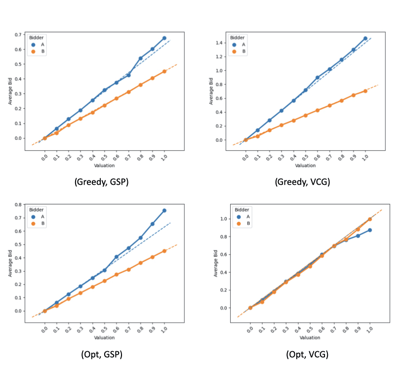
(a) Experiment 1: Mean bid by value. Dashes indicate theory.

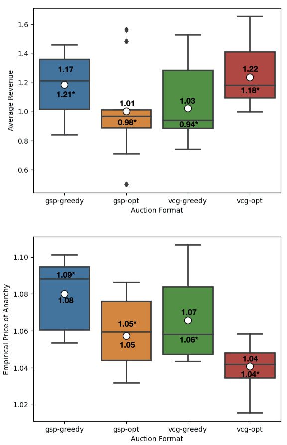
(b) Experiment 2: Fixed Valuations

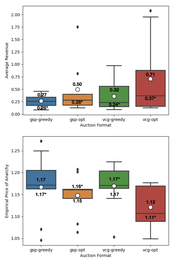
(c) Experiment 3: Random Valuations

Figure 1: Experimental Results. Scales differ due to normalization. Means (medians) are marked by circles (lines).

Experiments 2 and 3.

In Experiment 2, we use the Random Advertisers dataset. A protocol for a single round is as follows. We initialize an auction with 4 slots and 9 bidders of varying geometric discount factors (each with a fixed constant multiplier of $1$). Each bidder has a valuation drawn independently from the Random Advertisers dataset, and is initialized with a fresh exponential weights algorithm over the (discretized) bidspace up to their valuation, as we would expect bids to be conservative in practice. After an exploration period, the players update via EW for 100 rounds, updating their bid distributions based on the realized and counterfactual bids each round. Then, we sample a bid profile from the time-averaged joint distribution by uniformly selecting a time period and drawing a bid profile from the EW distributions of that given round; we average the revenue and welfare of 200 such samples as an estimate of the revenue and welfare given that valuation profile. For each auction format, we repeat this entire process for 200 total valuation profile draws, and average these together as an estimate of the format’s revenue and welfare under the valuation distribution. We also compute the optimal allocation for each draw, and take the ratio of the average optimal value to the average welfare as an estimate of an empirical analogue (i.e. not worst-case) to the PoA. We plot revenue and empirical PoA in Figure 1(b). Our third experiment is very similar to our second, except for the valuation sampling. Rather than sample valuations independently from the Random Advertiser dataset, we sample auctions randomly from the Random Auction dataset, and assign those bids to bidder valuations. Then we proceed as described in Experiment 1. We plot revenue and the Empircal PoA in Figure 1(c).

Experiment 2 and 3 Results.

In Experiment 2 (Figure 1(b)), a (rough) analog to the revenue hierarchy of Table 3 is apparent. Additionally, the Empirical PoAs of all formats are significantly better than the worst-case bounds in Table 1(a). In Experiment 3 (Figure 1(c)), the PoA is somewhat worse than those of Experiment 2, but again relatively far from the worst-case bounds we proved. On the other hand, the revenue hierarchy appears significantly different, with both GSP mechanisms doing worse than VCG. Together, these results suggest that the relative quality of mechanisms can be highly sensitive to the underlying distributions.

for $(\mathcal{A},\mathcal{P}_{\mathcal{A}})\in\{\text{[Greedy,Opt]}\times\text{(}[GSP,VCG])\}$ do

      for $t\in 1,2...,100$ do

           Draw 10 valuations. Initialize bidders with values and fresh Exp. Weights. for $t\in 1,2,...,1000$ do

                Initialize and run a 5 slot auction using $(\mathcal{A},\mathcal{P}_{\mathcal{A}})$ Draw bids and fix them. for $i\in\mathcal{I}$ do

                     for $b^{\prime}\in\{\frac{1}{d},\frac{2}{d},...,1\}$ do

                          Re-run auction with all other players’ bids fixed, but player $i$ using $b^{\prime}$.

                          Save payoff.

                         

                         Update ExpWeights.

                          end for

                         

                          end for

                         for $t^{\prime}\in 1,2,...100$ do

                               Test for CCE. If not, re-run another 1000 learning steps.

                               Draw number uniformly at random from the total number of learning steps to become round number.

                               Draw bid for each bidder from time average of ExpWeights at that round.

                               Run auction with these bids

                               Save round info.

                               end for

                              

                               end for

                              

                               end for

                              

                               end for

Algorithm 1 Protocol for Experiment 1

6 Discussion and Open Questions

In this paper, we obtain several theoretical and empirical results for the Ad Types setting. We leave several open directions. In terms of Price of Anarchy: while we provide constant upper and lower bounds on the Price of Anarchy under greedy allocation, there remains a gap between these bounds. More substantially, while we provide a constant lower bound on the Price of Anarchy under optimal allocation with VCG pricing, our upper bound is instance-dependent and likely quite pessimistic; resolving this with either a constant upper bound, or identifying a family of arbitrarily bad examples, would be helpful. In terms of equilibrium characterization, it would be useful to identify (or rule out) analytical solutions in more complicated settings. In terms of empirics: understanding how our results would change as various features of the setting change would be valuable. For instance, even our large setting is still relatively small compared to modern instances encountered in online advertising today. Second, our understanding of how revenue and welfare may vary with discount curves in practice is not yet systematic; theory suggests that bidders ought to bid less aggressively as their valuation of further slots increase, but how much less aggressively, and how this is affected by auction format, is unknown.

Appendix A Notation Table

References

- [1] Abrams, Z., Ghosh, A., and Vee, E. Cost of conciseness in sponsored search auctions. In Proc. of 3rd International Conference on Web and Internet Economics (2007), pp. 326–334.
- [2] Ausubel, L. M., and Milgrom, P. The lovely but lonely vickrey auction. In Combinatorial Auctions, chapter 1 (2006), MIT Press.
- [3] Caragiannis, I., Kaklamanis, C., Kanellopoulos, P., Kyropoulou, M., Lucier, B., Leme, R. P., and Tardos, É. Bounding the inefficiency of outcomes in generalized second price auctions. Journal of Economic Theory 156 (2015), 343–388.
- [4] Cavallo, R., Sviridenko, M., and Wilkens, C. A. Matching auctions for search and native ads. In Proceedings of the 2018 ACM Conference on Economics and Computation (2018), pp. 663–680.
- [5] Cavallo, R., and Wilkens, C. A. Gsp with general independent click-through-rates. In Proc. of 10th International Conference on Web and Internet Economics (2014), T.-Y. Liu, Q. Qi, and Y. Ye, Eds., pp. 400–416.
- [6] Chawla, S., and Hartline, J. D. Auctions with unique equilibria. In Proceedings of the fourteenth ACM conference on Electronic commerce (2013), pp. 181–196.
- [7] Chen, X., Deng, X., and Teng, S.-H. Settling the complexity of computing two-player nash equilibria. Journal of the ACM (JACM) 56, 3 (2009), 1–57.
- [8] Clarke, E. H. Multipart pricing of public goods. Public choice 11, 1 (1971), 17–33.
- [9] Colini-Baldeschi, R., Leonardi, S., Schrijvers, O., and Sodomka, E. Envy, regret, and social welfare loss. In Proceedings of The Web Conference 2020 (2020), pp. 2913–2919.
- [10] Colini-Baldeschi, R., Mestre, J., Schrijvers, O., and Wilkens, C. A. The ad types problem. In Web and Internet Economics: 16th International Conference, WINE 2020, Ljublana, Slovenia, December 17–20, 2017, Proceedings (2020), Springer.
- [11] Edelman, B., Ostrovsky, M., and Schwarz, M. Internet advertising and the generalized second-price auction: Selling billions of dollars worth of keywords. American economic review 97, 1 (2007), 242–259.
- [12] Feng, Z., Guruganesh, G., Liaw, C., Mehta, A., and Sethi, A. Convergence analysis of no-regret bidding algorithms in repeated auctions. In The Thirty-Fifth AAAI Conference on Artificial Intelligence (AAAI-21) (2021).
- [13] Forges, F. Five legitimate definitions of correlated equilibrium in games with incomplete information. Theory and decision 35, 3 (1993), 277–310.
- [14] Gomes, R., and Sweeney, K. Bayes–nash equilibria of the generalized second-price auction. Games and economic behavior 86 (2014), 421–437.
- [15] Groves, T. Incentives in teams. Econometrica: Journal of the Econometric Society (1973), 617–631.
- [16] Hartline, J., Syrgkanis, V., and Tardos, E. No-regret learning in bayesian games. In Advances in Neural Information Processing Systems (2015), pp. 3061–3069.
- [17] Kaplan, T. R., and Zamir, S. Asymmetric first-price auctions with uniform distributions: analytic solutions to the general case. Economic Theory 50, 2 (2012), 269–302.
- [18] Kleinberg, R. D., Ligett, K., Piliouras, G., and Tardos, É. Beyond the nash equilibrium barrier. In ICS (2011), pp. 125–140.
- [19] Kuhn, H. W. The hungarian method for the assignment problem. Naval research logistics quarterly 2, 1-2 (1955), 83–97.
- [20] Leme, R. P., and Tardos, E. Pure and bayes-nash price of anarchy for generalized second price auction. In 2010 IEEE 51st Annual Symposium on Foundations of Computer Science (2010), IEEE, pp. 735–744.
- [21] Lucier, B., and Paes Leme, R. GS0p auctions with correlated types. In Proceedings of the 12th ACM conference on Electronic commerce (2011), pp. 71–80.
- [22] Munkres, J. Algorithms for the assignment and transportation problems. Journal of the society for industrial and applied mathematics 5, 1 (1957), 32–38.
- [23] Roughgarden, T. Intrinsic robustness of the price of anarchy. Journal of the ACM (JACM) 62, 5 (2015), 1–42.
- [24] Roughgarden, T. Twenty lectures on algorithmic game theory. Cambridge University Press, 2016.
- [25] Roughgarden, T., Syrgkanis, V., and Tardos, E. The price of anarchy in auctions. Journal of Artificial Intelligence Research 59 (2017), 59–101.
- [26] Syrgkanis, V., and Tardos, E. Composable and efficient mechanisms. In Proceedings of the forty-fifth annual ACM symposium on Theory of computing (2013), pp. 211–220.
- [27] Varian, H. R. Position auctions. international Journal of industrial Organization 25, 6 (2007), 1163–1178.
- [28] Vickrey, W. Counterspeculation, auctions, and competitive sealed tenders. The Journal of finance 16, 1 (1961), 8–37.