Chalcogenic orbital density waves in weak and strong coupling limit

Abstract

Stimulated by recent works highlighting the indispensable role of Coulomb interactions in the formation of helical chains and chiral electronic order in the elemental chalcogens, we explore the $p$-orbital Hubbard model on a one-dimensional helical chain. By solving it in the Hartree approximation we find a stable ground state with a period-three orbital density wave. We establish that the precise form of the emerging order strongly depends on the Hubbard interaction strength. In the strong coupling limit, the Coulomb interactions support an orbital density wave that is qualitatively different from that in the weak-coupling regime. We identify the phase transition separating these two orbital ordered phases, and show that realistic values for the inter-orbital Coulomb repulsion in elemental chalcogens place them in the weak coupling phase, in agreement with observations of the order in the elemental chalcogens.

I Introduction

I.1 Orbital versus spin and charge density waves

It is well-known that spin- or charge-density waves can form in the ground states of Hubbard models. Such density waves are triggered by the Coulomb repulsion, which, together with appropriate nesting conditions, opens a gap in the electronic band structure at the Fermi level and stabilizes the spin or charge density waves at specific fillings. Perhaps one of the best-known examples here are the spin and charge density waves of the extended single-band one-dimensional (1D) Hubbard model at half-filling [1, 2, 3]. These become stable at infinitesimally weak interactions. Moreover, their physics in the weak- and strong-coupling limits, although distinct in details, is qualitatively similar.

Here we investigate a distinct type of density wave: the orbital density wave, consisting of a periodic modulation of the distribution of electrons between orbitals, keeping the charge and spin densities constant. We establish that this type of orbital density wave emerges as the ground state of a particular Hubbard model with orbital degrees of freedom. We show that considering a realistic orbital Hubbard model yields orbital order in a way that is qualitatively distinct from the typical spin and charge density waves.

I.2 Orbital density wave in the chalcogens

In contrast to the orbital order established in Mott insulators, like the cooperative Jahn-Teller effect [4], orbital density waves are currently known to exist in only a few materials. Whereas there have been suggestions that some of the dichalcogenides, such as for example 1T-TiSe₂ or 2H-TaS₂, can support orbital density waves [5, 6], perhaps the simplest case concerns the two elemental chalcogens— selenium and tellurium [7, 8, 9, 10]. Selenium and tellurium crystals have long been known to be semiconducting and to consist of weakly coupled helical chains of atoms, accompanied by a ‘chiral order’, at ambient pressure [11, 12, 13, 14] —though at high pressure both elements superconduct [15, 16].

The formation of helices naturally introduces spatially anisotropic electron hopping, which combines with the presence of an open $p^{4}$ valence subshell in chalcogenic atoms to give rise to the orbital density wave [11, 12, 17]. This sets the stage for explaining the formation of orbital density wave order using only a non-interacting model. This is referred to as a ‘valence bond’ mechanism [7], since it originates in the lowering of electronic kinetic energy in the 1D tight-binding model for the helical chain by a specific hybridization pattern of valence electrons between neighbouring orbitals. To be precise, on each chalcogen atom two valence electrons are assumed to reside in the two different $p$ orbitals that can hybridize with states on neighboring sites in the chain, while two other valence electrons known as the ‘lone pair’ occupy a the remaining $p$ orbital. The pattern of orbital occupancy obtained in this simple picture is shown in Fig. 1(a), and referred to as a ‘2-1-1’ orbital density wave.

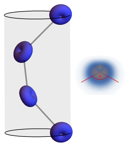
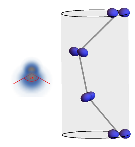
  (a)                                                                              (b)

Figure 1: Visualisation of two possible orbital density waves with period-3 that can in principle become stable in the helical chains of elemental chalcogens: (a) The ‘2-1-1’ orbital density wave with two orbitals being partially unoccupied, a configuration stable already in the non-interacting case; (b) The ‘2-2-0’ orbital density wave with one type of $p$ orbital unoccupied and supported by the inter-orbital Coulomb repulsion. Depicted here is the probability density for the wave function of the unoccupied orbital, with stronger opacity indicating a higher probability density as obtained in this paper for the orbital Hubbard model (1) with Coulomb repulsion $U=0$ [panel (a)] and using the Hartree approximation for $U=20t_{\sigma}$ [panel (b)], with $t_{\sigma}$ being the largest hopping element in the helical chain. The bond angle in Eq. (1) is here taken to be $\alpha=103^{\circ}$, while the hopping amplitudes obey $t_{\pi}=-t_{\sigma}/3$.

I.3 The role of Coulomb repulsion

Although the above discussion may suggest that there are no fundamental questions related to the onset of the orbital density wave in the chalcogens, let us now make a ‘detour’ and try to understand why the weakly coupled helical chains are formed in elemental chalcogens. Note that naively one would assume both elements to crystallise in a simple cubic structure [7, 8, 10]. To resolve this issue a minimal 3D microscopic model [10], which builds on earlier models [7, 8], was recently proposed. It starts with the Peierls effect which triggers the formation of charge density waves with period three in the three ‘straight’ chains formed by the $p_{\alpha}$ orbitals along each of the $\alpha=x,y,z$ cubic directions, accompanied by the formation of short and long bonds in those chains.

Next, a very small [18] inter-orbital Coulomb repulsion $U$ is invoked to explain the ‘locking’ of the respective phases of each of the charge density waves. Then, taking into account the electronic hopping processes solely across the short bonds naturally leads to the separation of the original 3D system into quasi-1D helical chains. Altogether, this leads to no net charge modulation per chalcogen atom [7, 10] and thus the charge density waves from all orbital channels combine to form orbital density waves in helical chains, see Fig. 1 of [10].

Within this picture, the helical chain thus necessarily has a nonzero inter-orbital Coulomb repulsion which stabilises an orbital density wave—however, basic calculations within a spinless model suggest (cf. Fig. 1 of [10]) that this density wave consists of a ‘2-2-0’ pattern with two ‘lone pairs’ and one empty orbital on each chalcogen atom, as shown in Fig. 1(b).

The purpose of this paper is to investigate the apparent inconsistency between the two models discussed above. Whereas the 1D tight-binding model supports the onset of a ‘2-1-1’ orbital density wave in each helical chain, the 3D model with finite electron-phonon and inter-orbital Coulomb repulsion explains the formation of helical chains but gives rise to a ‘2-2-0’ orbital density wave. In particular, it is clear that if the presence of helical chains in the crystal structure of elemental chalcogens indeed relies on the presence of Coulomb interactions, these should be included in any realistic electronic model.

This leads us to address two questions: (i) What is the critical value of the Coulomb repulsion $U_{\rm crit}$ which triggers the onset of the (unrealistic) ‘2-2-0’ orbital density wave in the helical chain? (ii) What is a realistic value of the inter-orbital Coulomb repulsion in the chalcogens—is it smaller than $U_{\rm crit}$ so that, despite the finite Coulumb repulsion, the model for the electronic band structure of the helical chains can still support the ‘2-1-1’ orbital density wave that is indirectly observed in the chalcogens? Note that the answer to the above questions cannot be easily predicted by some kind of back-of-the-envelope calculations; for instance, in the well-known case of the extended Hubbard model [1, 2, 3], both the charge and spin density waves are stabilised already by an infinitely small Hubbard $U$, so that $U_{\rm crit}=0$.

To study the role of Coulomb repulsion in the formation of the orbital density wave in the two elemental chalcogens, we first formulate a particular $p$-orbital Hubbard model on a 1D helical chain, see Sec. II. We then turn to the Hartree approximation, which is used to obtain solutions in both the weak and strong-coupling regimes, see Sec. II.3. In Sec. III.1 we present the results of the tight binding model which are extended by the effect of $U$ in Sec. III.2. The results are discussed in Sec. IV. First, the orbital density wave is visualized in Sec. IV.1. Next we interpret the results obtained in the weak-coupling (Sec. IV.2) and strong-coupling (Sec. IV.3) limits. We discuss the qualitative differences between the orbital density waves found in the different regimes of coupling strength in Sec. IV. The paper is summarized in Sec. V, while we derive the nearest neighbor hopping matrix in Appendix A and verify the employed Hartree approximation using the preliminary density matrix renormalization group (DMRG) simulations in Appendix B.

II Model and Methods

Since the late 1940’s, it has been known that the crystal structure of trigonal selenium and tellurium consists of loosely-coupled, 1D, helical chains [11]. It can be thought of as a deformation of a hypothetical ‘parent’ cubic lattice in which the bond angles are enlarged along helical paths through the cubic structure, as shown schematically in Fig. 2 [19, 20, 21, 22]. This yields a helical chain with a period of three bonds ($\lambda=3$). For both selenium and tellurium, the bond angle $\alpha$ has been experimentally determined to be $\alpha\approx 103^{\circ}$ [11, 22].

Both selenium and tellurium are group-16 elements (chalcogens) with the electron configuration $ns^{2}\,np^{4}$. Consequently, on each chalcogen ion in the helical chain we consider a 2/3 filled $p$-shell. To be able to explore both the influence of electron-electron interactions and chain geometry on orbital order in these chains, we will construct a spinless three-orbital Hubbard model. We neglect the spin degree of freedom both to simplify the model and because spin is not expected to play an important role in selenium and tellurium [18] —see also the discussion at the end of Sec. V. The Hamiltonian then consists of two terms—the hopping or kinetic term $H_{t}$ and the interaction term $H_{U}$,

$$H=H_{t}+H_{U}.$$ (1)

II.1 The kinetic energy

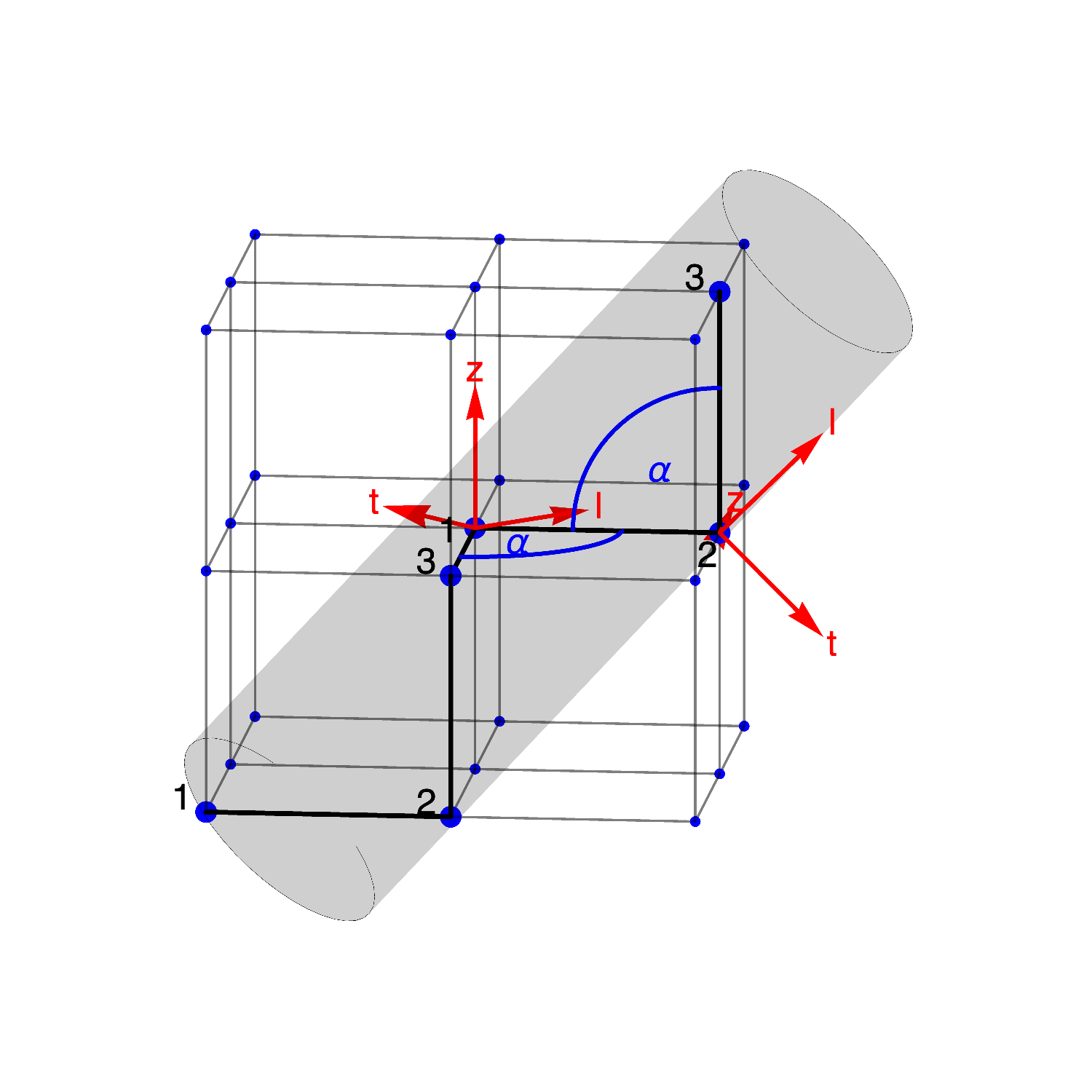
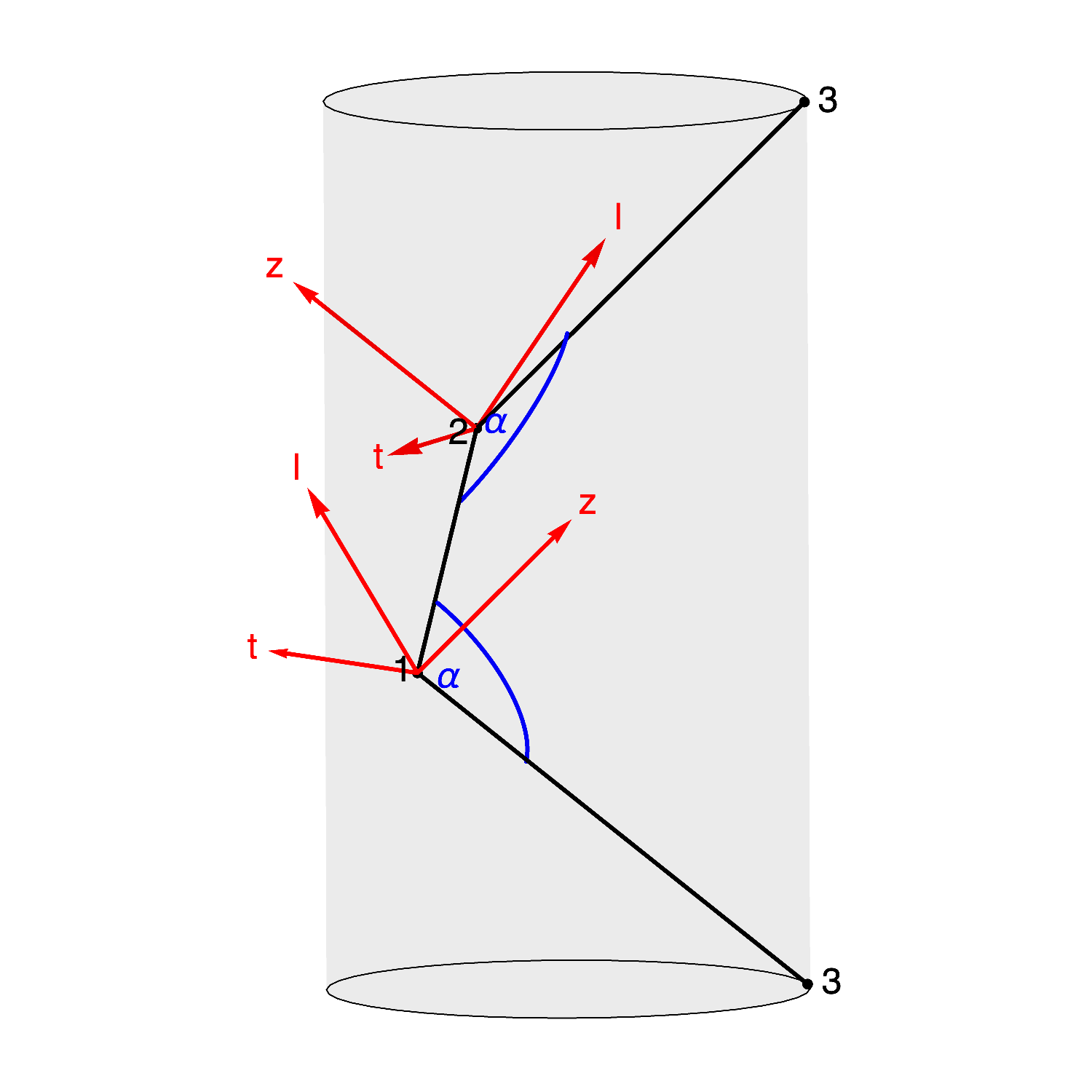
(a)      (b)

Figure 2: The helical chains in elemental chalcogens visualized in two possible geometries: (a) the idealised simple cubic case with $\alpha=90^{\circ}$; (b) the realistic case with $\alpha>90^{\circ}$ (the selenium/tellurium structure is obtained for the bond angle $\alpha=103^{\circ}$). Indicated in each case are three atoms in a single ($\lambda=3$) period of the chain, the bond angles $\alpha$, and the local basis in relation to the bond angle. Looking along the chain, the three atoms form an equilateral triangle. The projection of the distance between neighboring atoms onto the chain axis depends on the bond angle.

Formally, we can write

$$H_{t}=\sum_{i,\mu,\nu}\left(T_{\mu,\nu}(i)c^{\dagger}_{i,\mu}c_{i+1,\nu}+H.c.\right),$$ (2)

where $c^{\dagger}_{i,\mu}$ ($c_{i+1,\nu})$ creates (annihilates) a spinless electron with orbital $\mu$ $(\nu)$ on site $i$ $(i+1)$ along a helical chain. The orbital indices enumerate the three orthogonal $p$ orbitals at each site. The tunneling amplitudes between orbitals on neighboring sites are encoded in the hopping matrix $T_{\mu,\nu}(i)$ and depend on the Slater-Koster overlap integrals between the nearest neighbor $p$ orbitals [23],

$$t_{\sigma}\equiv(pp\sigma),\hskip 28.45274ptt_{\pi}\equiv(pp\pi).$$ (3)

Here we use $t_{\sigma}=2.57$ eV [19] and $t_{\pi}=-t_{\sigma}/3$ [12]. Note that the hopping matrix depends on the site index $i$, because the helical chain has three non-equivalent sites.

To derive an explicit form for the hopping matrix $T_{\mu,\nu}(i)$, we first need to choose an orbital basis $\{p_{\mu}\}$. The two most general choices include either picking a global basis, the same at each site, or considering a set of three local bases—one for each site in a single period of the chain. The Hubbard problem is much simpler if one makes the second choice, because the helical symmetry can then by used to render the orbital orientations relative to surrounding atoms the same at each site.

To this end, we choose each local basis in such a way that the lobes of each of the three $p_{\mu}\equiv\{p_{x},p_{y},p_{z}\}$ orbitals are parallel to the axes of a local Cartesian coordinate system. The local coordinates are defined by a set of three unit vectors $\{{\bf l},{\bf t},{\bf z}\}$ which fulfill the conditions that: (i) ${\bf z}={\bf l}\times{\bf t}$, (ii) both ${\bf l}$ and ${\bf t}$ lie in the same plane as the bond angle $\alpha$, (iii) ${\bf l}$ is perpendicular to the bisector of the bond angle $\alpha$ and points towards the neighboring site with highest site index, and (iv) ${\bf t}$ is parallel to the bisector of the bond angle $\alpha$ and points outwards from the bond angle $\alpha$. Two examples of the local coordinate systems, in relation to the bond angle $\alpha$, are presented in Fig. 2.

This choice of local basis leads to the nearest neighbor hopping matrices $T_{\mu,\nu}(i)$ being the same for each site $i$. Consequently, instead of working with a $(9\times 9)$ hopping matrix in the global basis (three sites with three orbitals), we only need to consider a $(3\times 3)$ hopping matrix in the local basis (one site with three orbitals). The trade-off in this approach is that one needs to specifically derive the elements of the matrix $T_{\mu,\nu}$ in terms of the bond angle $\alpha$ and the hopping amplitudes $\{t_{\sigma},t_{\pi}\}$. Making use of the helical symmetry, this is a straightforward but tedious procedure, described in detail in the Appendix.

The resulting matrix elements can be linearized with respect to the bond angle, around $\alpha=90^{\circ}$, which does not change the bandwidth by more than 15% for $\alpha$ in the range $[90^{\circ},105^{\circ}]$ (see Appendix). The linearized hopping matrix is given by

$$T_{\mu,\nu}=\frac{1}{2}\!\left(\begin{array}[]{ccc}(1+\epsilon)\,t_{\sigma}+\epsilon\,t_{\pi}&t_{\sigma}-\epsilon\,t_{\pi}&\frac{2-\epsilon}{\sqrt{2}}\,t_{\pi}\\ -\,t_{\sigma}+\epsilon\,t_{\pi}&(-1+\epsilon)\,t_{\sigma}-\epsilon\,t_{\pi}&\frac{2+\epsilon}{\sqrt{2}}\,t_{\pi}\\ \frac{2-\epsilon}{\sqrt{2}}\,t_{\pi}&-\frac{2+\epsilon}{\sqrt{2}}\,t_{\pi}&-2\epsilon\,t_{\pi}\\ \end{array}\right)\!.$$ (7)

Here $\epsilon=\alpha-\pi/2$ denotes the deviation from the simple cubic arrangement.

To build intuition, we first consider the special case of $\epsilon=0$, in the limit of $t_{\pi}=0$ (realistic $t_{\pi}$ in selenium/tellurium is expected to be around $-t_{\sigma}/3$). The non-vanishing hopping amplitudes then form a $2\times 2$ block within the matrix $T_{\mu,\nu}$:

$$T_{\mu,\nu}(t_{\pi}=0,\alpha=90^{\circ})=\frac{1}{2}\,t_{\sigma}\left(\begin{array}[]{ddd}\!\!$&$&0$\\ \!\!$&$&0$\\ 0\!\!$&0$&0$\end{array}\!\right)\!.$$ (9)

This result can be easily understood in terms of the simple cubic lattice structure.

Since $t_{\pi}=0$, the only possible hopping is between orbitals of the same flavor aligned along the bonds. The natural basis in this case is that of simple cubic crystal axes. In such a (global) basis the hopping matrix is bond dependent. As an example, let us focus on the bond extending along the $\hat{x}$ axis. The hopping matrix is very simple:

$$(T_{x})_{\mu,\nu}=t_{\sigma}\left(\begin{array}[]{ddd}$&0$&0$\\ 0$&0$&0$\\ 0$&0$&0$\end{array}\!\right)\!.$$ (10)

Looking at Fig. 2, one can see that the matrix in Eq. (9) is obtained by rotating the basis on the left by $45^{\circ}$ around the $\hat{z}$ axis, and the basis on the right by: (i) $-90^{\circ}$ around the $\hat{x}$ axis, (ii) $-45^{\circ}$ around the $\hat{y}$ axis. It is easy to check that one gets Eq. (9) as a result of these transformations applied to Eq. (10). One can of course perform the right rotations for other bonds and obtain Eq. (9) in each case.

II.2 The on-site Hubbard interaction

Since the change from the global to the local coordinate basis is just a local rotation, it does not affect the on-site interaction terms. The local Hubbard-$U$ repulsion between spinless electrons in different $p$ orbitals at the same site is thus written as

$$H_{U}=\,U\sum_{\scriptsize\begin{array}[]{c}\mu>\nu\\ \mu,\nu=l,t,z\end{array}}\!\sum_{i}\,n_{i,\mu}n_{i,\nu}.$$ (11)

Here we defined the number electron number operator, $n_{i,\mu}=c^{\dagger}_{i,\mu}c_{i,\mu}$ and took into account the well-known fact that the electron-electron coupling constant $U_{\mu,\nu}=U$ is the same for each pair of $p$ orbitals, cf. Refs [24, 25].

While in what follows we will treat the Hubbard $U$ as a model parameter and vary it, let us also estimate the realistic value of the inter-orbital Coulomb repulsion between two spinless electrons in the elemental chalcogens:

$$U_{\rm real} \simeq\frac{1}{4}\Big{[}F^{(0)}+\frac{1}{25}F^{(2)}\Big{]}+\frac{3}{4}\Big{[}F^{(0)}-\frac{1}{5}F^{(2)}\Big{]}$$

$$=F^{(0)}-\frac{14}{100}F^{(2)}$$

$$=U_{\rm Te}-\frac{7}{10}J_{\rm Te}$$

$$\approx 0.61\ {\rm eV}.$$ (12)

Here we assumed the following: (i) in the first line of Eq. (II.2) we approximated the effective inter-orbital repulsion between two spinless electrons by a repulsion between two spinful electrons either in an inter-orbital singlet (3 out of 12 possible ‘inter-orbital multiplets’) with energy $F^{(0)}+\frac{1}{25}F(2)$ or a triplet (9 out of 12 possible ‘inter-orbital multiplets’) with energy $F^{(0)}-\frac{1}{5}F(2)$ ($F^{(k)}$ are the Slater integrals defined in a standard way, cf. [25], and the calculations of atomic multiplets are for example available at https://www.cond-mat.de/sims/multiplet/); (ii) in the third line of Eq. (II.2) we introduced the values of the Coulomb repulsion parameters as estimated by Deng et al. for solid tellurium [26, 27]: $F^{(0)}=U_{\rm Te}\approx 1.10$ eV and $F^{(2)}/5=J_{\rm Te}\approx 0.7$ eV. Note that in this way we obtain a realistic ratio $U/t_{\sigma}\approx 0.24$ in tellurium and that this also constitutes the lower bound for that ratio for selenium—since the selenium $4p$ orbitals are effectively ‘smaller’ than the tellurium $5p$ orbitals and hence the value of the Slater integral $F^{(0)}$ should be larger in the former case.

II.3 The Hartree approximation

To solve the Hubbard model for the helical chain, we employ the Hartree approximation. This means that the interaction term becomes

$$H_{U}=U\!\sum_{\scriptsize\begin{array}[]{c}\mu>\nu\\ \mu,\nu=l,t,z\end{array}}\!\sum_{i} \>\Big{(}\langle n_{i,\mu}\rangle\>n_{i,\nu}+n_{i,\mu}\>\langle n_{i,\nu}\rangle$$ (15)

$$-\langle n_{i,\mu}\rangle\langle n_{i,\nu}\rangle\Big{)}.$$ (16)

Because the outer $p$-shell of chalcogen atoms is 2/3-filled, we expect to find two spinless electrons per site. The mean fields thus need to fulfill the following condition at every site $i$:

$$\sum_{\mu}\;\;\langle n_{i,\mu}\rangle\,=2.$$ (17)

To solve the mean field model consisting of Eqs. (2) and (15), we use the Ansatz that the ground state expectation values $\{\langle n_{i,\mu}\rangle\}$ have unbroken translational symmetry in the local basis. That is, we look for ground states within the subspace of translationally invariant eigenstates that obey:

$$\begin{array}[]{lr}\langle n_{i,\mu}\rangle\equiv\bar{n}_{\mu}&\text{for}\;\mu=l,t,z.\\ \end{array}$$ (18)

This assumption is equivalent to only considering types of order that respect the helical symmetry of the chain in the global coordinate basis. Consequently, the periodicity of the orbital density waves that we are looking for is encoded in our choice of local basis and the only unknown we need to solve for in the mean field analysis is the orbital occupation (again, in the local basis). As already discussed in the Introduction, physically this means that the presence of helical chains in the atomic structure of elemental chalcogens hardwires a preferred periodicity for any density wave instability. It does not, however, determine the amplitude and the form of any orbital density wave. That is, the choice of occupied orbitals resulting from the competition between the ‘2-1-1’ and ‘2-2-0’ density waves (corresponding to ’1-0.5-0.5’ and ’1-1-0’ ordering of spinless electrons) is still to be determined. These are influenced by the trigonal distortions (deviation of the bond angle $\alpha$ from 90^∘) and Coulomb repulsion (represented by the Hubbard $U$).

The orbital occupation numbers $\{\bar{n}_{\mu}\}$ can be solved for in a self-consistent manner. Namely, we look for the lowest energy fixed point of the recursion relations:

$$\left(\bar{n}_{l}\right)_{k} =\frac{1}{N}\sum_{q}\;\left<\Phi_{0}(\left(\bar{n}_{l}\right)_{k-1},\left(\bar{n}_{t}\right)_{k-1},U)\right|n_{q,l}\left|\Phi_{0}\left((\bar{n}_{l})_{k-1},\left(\bar{n}_{t}\right)_{k-1},U\right)\right>,$$

$$\left(\bar{n}_{t}\right)_{k} =\frac{1}{N}\sum_{q}\;\left<\Phi_{0}(\left(\bar{n}_{l}\right)_{k-1},\left(\bar{n}_{t}\right)_{k-1},U)\right|n_{q,t}\left|\Phi_{0}\left((\bar{n}_{l})_{k-1},\left(\bar{n}_{t}\right)_{k-1},U\right)\right>,$$

$$(\bar{n}_{z})_{k} =2-(\bar{n}_{l})_{k}-(\bar{n}_{t})_{k}.$$ (19)

Here, the state $\left|\Phi_{0}\left((\bar{n}_{l})_{k-1},(\bar{n}_{t})_{k-1},U\right)\right>$ used in calculating the mean field values in step $k$, is the ground state of the Hamiltonian defined by Eqs. (2) and (15) with mean field values $\langle n_{i,l}\rangle=\left(\bar{n}_{l}\right)_{k-1}$ and $\langle n_{i,t}\rangle=\left(\bar{n}_{t}\right)_{k-1}$, calculated in the step $k-1$ of the recursive procedure. We also used the fact that for a site-independent orbital occupation (in the local basis), we have

$$\left<\Phi_{0}\right|n_{i,\mu}\left|\Phi_{0}\right> =\frac{1}{N}\sum_{i}\left<\Phi_{0}\right|n_{i,\mu}\left|\Phi_{0}\right>$$

$$=\frac{1}{N}\sum_{q}\left<\Phi_{0}\right|n_{q,\mu}\left|\Phi_{0}\right>.$$ (20)

Note that the last equality in Eq. (II.3) directly follows from Eq. (17) and that this condition is also implicitly used in the first two equations in Eq. (II.3). The calculations are performed for a 100-site chain.

III Results

III.1 The tight binding model ($U=0$)

In the non-interacting model with $U=0$, i.e., considering only the hopping term of Eq. (2), the orbital occupations in the ground state $\{\bar{n}_{\mu}\}$ can be calculated exactly. In Fig. LABEL:non-interacting-results(a) we show that the $\{\bar{n}_{\mu}\}$ remain approximately constant for angles in the range $\alpha\in(90^{\circ},105^{\circ})$. The values at the selenium/tellurium bond angle are $\bar{n}_{l}\approx\bar{n}_{t}\approx 0.54$, and $\bar{n}_{z}\approx 0.92$. In Fig. LABEL:non-interacting-results(b) we show $\{\hat{n}_{\mu}\}$ as a function of bond angle $\alpha$ when $t_{\pi}=0$. As in the previous case, the occupation numbers do not change within the pictured bond angle range and are very simmilar to those obtained for realistic values of $t_{\pi}$.

Note that since both Figs. LABEL:non-interacting-results(a) and (b) have been calculated using the linearized hopping matrix, results obtained for bond angles higher than $\approx 105^{\circ}$ differ quantitatively from those obtained using the full hopping matrix. The experimentally established bond angles in selenium and tellurium, however, lie well within the region where the linear approximation is valid (as discussed in the Appendix).

The results obtained in the non-interacting limit fully agree with the ’valence bond picture’ (as described in Refs. [11, 12, 17]), which translates to (1,0.5,0.5) orbital occupancies in the spinless electron language. According to this mechanism, every chalcogen atom lends a single electron to each of two covalent bonds, while the other two electrons remain in the $p_{z}$ orbital, normal to the bond angle plane. In the spinless electron picture, this translates to one spinless electron distributed evenly between the two orbitals in the bond angle plane, $p_{l}$ and $p_{t}$, while the remaining electron occupies the $p_{z}$ orbital, as shown in Figs. LABEL:non-interacting-results(a) and LABEL:non-interacting-results(b). As presented in Sec. IV.1 and shown in Fig. 1, this leads to the orbital density wave of the ‘2-1-1’ character.

III.2 Including the interaction term

To study the properties of the full Hubbard model, including a non-zero Coulomb repulsion $U$, we employ the Hartree approximation described by Eq. (15). The resulting evolutions of the orbital occupation numbers $\{\bar{n}_{\mu}\}$, as well as the derivative of the ground state energy with respect to the Coulomb repulsion strength, $d\epsilon_{0}/dU$, are shown in Fig. LABEL:interacting-results. Increasing interaction strength leads to a phase transition, which occurs at $U_{\rm crit}\approx 2.8t_{\sigma}$ for both $t_{\pi}=-t_{\sigma}/3$ and $t_{\pi}=0$. It is signalled by discontinuities in $d\epsilon_{GS}/dU$ [see Fig. LABEL:interacting-results(c) and LABEL:interacting-results(d)] and orbital occupations $\{\bar{n}_{\mu}\}$ [see Fig. LABEL:interacting-results(a) and LABEL:interacting-results(b)].

For weak interactions ($U<U_{\rm crit}$), the obtained orbital density wave agrees with the one discussed in Sec. III.1 immediately above—see Figs. LABEL:non-interacting-results(a-b). Thus, the ‘valence bond picture’ is valid here and the ‘2-1-1’ character of the density wave is observed, see Sec. IV.1 and Fig. 1.

As the system approaches the critical value of the Coulomb repulsion $U_{\rm crit}$, the following effects are observed:

(i) in the bond-angle plane the hole occupation slightly polarizes, favoring the $p_{l}$ orbital, for both zero and non-zero $t_{\pi}$

(ii) perpendicular to the bond-angle plane the $p_{z}$ orbital is always occupied for $t_{\pi}=0$ [see Fig. LABEL:interacting-results(b)], while for nonzero $t_{\pi}$ its occupation is slowly increased with increasing interaction, without a visible discontinuity at the transition.

For interaction strengths slightly above $U_{\rm crit}$, the system is approaching a saturated state, with a least-occupied $p_{t}$ orbital character. The occupation numbers change slowly upon further increasing $U$, so that in the infinite $U$ limit the spinless electrons are completely localized on the $p_{t}$ and $p_{z}$ orbitals. This gives (1,1,0) orbital occupation in the spinless electron model, which, as presented in Sec. IV.1 and Fig. 1, characterizes the orbital density wave of ‘2-2-0’ character.

IV Discussion

IV.1 Visualising the orbital density waves

Having found the ground state of the mean field model in the local basis, we can translate it back to the global basis. This allows us to clearly present the real-space orbital densities in selenium/tellurium chains, as shown already in Fig. 1 of the Introduction, for both $U<U_{\rm crit}$ and $U>U_{\rm crit}$. The phases in these regimes differ significantly in the way electronic charge is distributed over the orbitals.

The orbital density wave stabilized in the non-interacting case and for all values of $U<U_{\rm crit}$, has two ($p_{l}$ and $p_{t}$) partially occupied orbitals lying in the bond angle plane, i.e. the orbital density wave has ‘2-1-1’ character (one orbital fully occupied and two partially occupied), and is qualitatively similar to the one depicted in Fig. 1(a). Interestingly, we observe that the resulting charge density is flattened in the direction normal to the bond angle (the $z$ direction in the local basis). Above the critical interaction strength $U>U_{\rm crit}$ the system enters a different phase and the unoccupied orbital is purely of $p_{t}$ character as shown for $U=20t_{\sigma}$ in Fig. 1(b). In the ‘spinful language’ this density wave corresponds to the so-called ‘2-2-0’ orbital density wave (two orbitals fully occupied and one empty).

IV.2 Orbital density wave for $U<U_{\rm crit}$

To understand the presence of an orbital density wave for $U<U_{\rm crit}$, it suffices to consider the exactly solvable non-interacting case. The evolution of the orbital occupation with bond angle can be then understood entirely in terms of the evolution of the band structure, which is shown in Fig. LABEL:non-interacting-bands.

In the simple cubic case, obtained for the bond angle $\alpha=90^{\circ}$, we see three well-separated, three-fold degenerate bands [see Fig. LABEL:non-interacting-bands(a)]. The middle three degenerate bands can be identified as having mostly $p_{z}$ orbital character, while the other two three-fold degenerate bands are formed by linear combinations of the $p_{l}$ and $p_{t}$ orbitals lying in the bond angle plane. The degeneracy of the bands is a consequence of the $\alpha=90^{\circ}$ bond angle, for which there exists a global orbital basis in which there is absolutely no orbital mixing, even with nonzero $t_{\pi}$. This is the basis associated with the three cubic crystal axes.

For bond angles $\alpha>90^{\circ}$, the degeneracy is lifted and for the selenium/tellurium bond angle $\alpha=103^{\circ}$ nine distinct bands can be seen [see Fig. LABEL:non-interacting-bands(b)]. Nevertheless, they are well separated into three classes of bands. The insulating character remains for the present filling of 2/3 but the gap is somewhat reduced.

IV.3 Orbital density wave for $U>U_{\rm crit}$

To understand the orbital density wave in the strong-coupling limit, with $U>U_{\rm crit}$, we focus on the infinite $U$ limit. Within the Hartree approximation, a phase transition occurs when one of two things happens in the flow of the iterative procedure defined by Eq. (II.3): (i) either a new fixed point appears, which is also a new global energy minimum, or (ii) the energy hierarchy of existing fixed points changes, thus switching the ground state. To investigate which case is realized here, Fig. LABEL:fixed-points depicts the flow diagrams and fixed points for four values of the interaction strength.

First, in Fig. LABEL:fixed-points(a), the non-interacting model is seen to have a single fixed point. As $U$ increases, the fixed point moves towards the $\bar{n}_{t}=1-\bar{n}_{l}$ axis [see Fig. LABEL:fixed-points(b)]. This is visible as a continuous increase of $\bar{n}_{z}$ as $U$ departs from zero in Figs. LABEL:interacting-results(a) and LABEL:interacting-results(c). Eventually, for $U=U_{\rm crit}$, the single fixed point vanishes, while three new ones emerge near the corners of parameter space, as shown in Fig. LABEL:fixed-points(c). The new ground state is in the corner $\bar{n}_{t}\approx 0$ and $\bar{n}_{l}\approx 1$. This is the saturated phase with an unoccupied $p_{t}$ orbital.

For even larger values of $U$, the three fixed points move further towards the corners of parameter space [Fig. LABEL:fixed-points(d)], where they settle and become degenerate in the $U\rightarrow+\infty$ limit. Incidentally, these corner states constitute the three-fold degenerate ground state of the inter-orbital Coulomb repulsion on a single chalcogen ion in the $\{p_{l},p_{t},p_{z}\}$ basis.

In the full 1D Hubbard model (1) the three-fold degeneracy of the ground state in the infinite $U$ limit is broken by the kinetic term (2), whcih leads to the selection of $p_{t}$ as the single least-occupied orbital. This means that whereas the Coulomb repulsion triggers the onset of the orbital density wave in the strong coupling limit, the kinetic term decides on the precise nature of the orbital density wave.

V Conclusions

V.1 Summary of main results

In this paper we studied the instabilities towards orbital density wave order in a $p$-orbital Hubbard model for a helical chain. This is the relevant geometry for the trigonal phases of the two elemental chalcogens selenium and tellurium [11, 12, 22, 19, 13]. By considering the orbital Hubbard model for such a helical chain in the Hartree approximation, we showed that an orbital density wave with the same period as the atomic helix is stabilised, irrespective of the strength of the inter-orbital Coulomb repulsion $U$. The precise form of the orbital density wave, however, is strongly sensitive to the interaction strength $U$. For realistic values of both the bond angle in the helical chain and the ratio of the hopping amplitudes $t_{\pi}$ and $t_{\sigma}$, we observe a phase transition between qualitatively different orbital density waves at $U_{\rm crit}\approx 2.8t_{\sigma}$.

As the main result of this work, we have shown that in the considered model the value of $U_{\rm crit}$ is not only nonzero, but also relatively large—and that the estimated value of $U_{\rm real}\approx 0.24t_{\sigma}$ in the two elemental chalcogens clearly puts these materials in the weak-coupling regime, with $U_{\rm real}<U_{\rm crit}$. Therefore, the stable orbital density wave in the chalcogen model with a finite but realistic Hubbard $U$ can be adiabatically connected to the ground state of the model without Coulomb interactions. We thus show that including a realistic value of inter-orbital Coulomb repulsion does not invalidate the paradigm of the ‘valence bond picture’ [11, 12, 17] [i.e. the ‘2-1-1’ density wave of Fig. 1(a)] in the helical chalcogens: The orbital density variations are already imposed by the combination of the helical chain structure and the anisotropic hopping amplitudes of the $p$ orbitals. The sole role of the relatively small inter-orbital Coulomb repulsion in the chalcogens is to explain the formation of the helical chains themselves, starting from a hypothetical cubic crystal, as postulated in [10].

It is only in the limit of unrealistically strong interactions with $U>U_{\rm crit}$ that we find a distinct orbital density wave, with only one type of orbital being unoccupied per chalcogen, i.e., the ‘2-2-0’ density wave of Fig. 1(b). While the orbital density wave in the strong-coupling limit is triggered by the on-site Coulomb repulsion $U$, and can be easily understood in the fully localised limit of infinite $U$, the particular choice of the orbital which is occupied by a single hole is dictated by the kinetic energy.

V.2 Relevance of the employed model and approximation

Let us first comment on the role of the spin degree of freedom, neglected in this study. In some of the previous works [7, 8, 27, 26] on the subject it was postulated that the Hund’s exchange could be the dominant mechanism which stabilises the double occupancy of one of the valence $p$ orbitals and partial occupancy of the other two orbitals on each chalcogen atom; in this way the ‘2-1-1’ density wave should be easily supported in the chalocogens. While it is natural to expect that the Hund’s exchange may support the ‘2-1-1’ orbital density wave, this work, in combination with Ref. [10], shows that, even without taking into account the electron’s spin and Hund’s exchange, both the helical structure and the orbital density wave can be stabilised in elemental chalcogens. Although detailed further studies are needed here, the results shown here suggest that in the real materials the role of spin and Hund’s exchange may also be secondary. In fact, to the best of our knowledge, there are no reports of any onset of spin density modulations in elemental chalcogens. We remark that such modulations would indeed be expected if the spin degree of freedom mattered for the onset of the orbital density wave.

Next, let us discuss the validity of the Hartree approximation. In this case it is worth pointing out that even in the case of the 1D single-band (i.e., ‘standard’) Hubbard model at half-filling, the Hartree approximation leads to a partially correct result, especially in the weak-coupling limit [28]. Moreover, we expect that for the (anisotropic) orbital Hubbard model studied here, which lacks a continuous symmetry in the orbital sector, the Hartree approximation should work better, for the quantum fluctuations should then be somewhat suppressed. Nevertheless, in order to check this presumtion, we performed preliminary DMRG calculations of the orbital Hubbard model, see Appendix B for further details.

Crucially, the obtained DMRG results unambiguously confirm that the ‘2-1-1’ orbital density wave is indeed stable in the weak-coupling limit—in particular, this density wave is the ground state well above the realistic value of $U=0.2t_{\sigma}$. On the other hand, the ‘2-2-0’ orbital density wave, i.e. the density wave that is not observed in the chalcogens and that—according to the Hartree approximation—could become stable in the limit of unrealistically high Hubbard $U$ (see above), seems to be further destabilised in the DMRG simulations. In fact, according to the preliminary DMRG calculations, this density wave becomes stable only once a small crystal field, that has not been included in the model considered in this paper, but may nevertheless be present in the 3D chalcogens (see Appendix B), is added. Note that, in order to unequivocally verify the stability of the ‘2-2-0’ orbital density wave as well as to further corroborate the phase diagram of the orbital Hubbard model proposed here, further, extensive numerical studies are needed (due to the numerical complexity of the orbital Hubbard model these are beyond the scope of this work).

Finally, we note that the effects of the electron-phonon coupling are in general neglected here and left for future studies. Nevertheless, we stress that the mere onset of the 1D helical chains in the chalcogens originates in a particular electron-phonon coupling, see [10] and discussion in Sec. I.3.

V.3 Final remarks

The discussed here emergence of the different types of orbital order shows how the physics of the 1D $p$-orbital Hubbard model in a helical chain differs from that of the single-band Hubbard model in one dimension which may host spin or charge density waves. In general terms, the reason for this is two-fold: First, the orbital systems are naturally prone to lattice distortions due to the strong coupling between orbitals and lattice. One should then consider the lattice distortions (such as the ones leading to helical chains in elemental chalcogens) before deriving the physically-relevant, orbital Hubbard model. Second, unlike those in the single-band Hubbard model, the hopping amplitudes between distinct orbitals are generically strongly anisotropic, triggering spatial dependencies in observable quantities and phenomena.

Appendix A The hopping matrix

In this Appendix, we derive the nearest neighbor hopping matrix ${T}_{\mu,\nu}(i)$—here referred to as $\hat{T}(i)$. Since the chain has a helical symmetry, it suffices to consider a single bond to derive all the hopping elements in the chain or, phrasing it differently, in the local basis the hopping matrix $\hat{T}(i)$ is site-independent and we can drop the site index: $\hat{T}(i)\equiv\hat{T}$ (as discussed in the main text).

To describe a bond, we consider two neighboring sites in the chain and label them $1$ and $2$. In order to find the local basis on site 2 one needs to take the local basis on site 1 and rotate it by $-{2\pi}/{3}$ around the helical axis, as shown in Fig. 2. In the local basis, the helical axis is related to the local ${\mathbf{z}}$ axis via a rotation by $\beta$ around the local ${\mathbf{t}}$ axis [see Fig. 2(b)]. The angle $\beta$, in turn, can be written in terms of the bond angle $\alpha$ as:

$$\cos\beta=\tan\left(\frac{\pi}{6}\right)\tan^{-1}\left(\frac{\alpha}{2}\right).$$ (21)

Consequently, the basis change from the local basis at site 1 to the local basis at site 2 is:

$$\hat{R}_{1,2}=\hat{R}_{t}(\beta)\,\hat{R}_{z}\left(-\frac{2\pi}{3}\right)\,\hat{R}_{t}^{{\dagger}}(\beta).$$ (22)

Finally, the vector pointing along the bond from site $1$ to site $2$ is rotated by $\left({\alpha}-{\pi}\right)/2$ around the local ${\mathbf{z}}$ axis with respect to basis vector $\mathbf{l}$ of the local basis at site $1$.

Since the $p$ orbitals transform like vectors under rotations, all of the above leads to the following expression for the hopping matrix

$$\hat{T}=\hat{R}_{z}\left(-\frac{\alpha}{2}+\frac{\pi}{2}\right)^{{\dagger}}\,\hat{T}_{0}\,\hat{R}_{z}\left(-\frac{\alpha}{2}+\frac{\pi}{2}\right)\,\hat{R}_{1,2}.$$ (23)

Here $\hat{T}_{0}$ is the hopping matrix for the $p$ orbitals in a straight 1D chain, given by:

$$\hat{T}_{0}=\left(\begin{array}[]{ccc}t_{\sigma}&0&0\\ 0&t_{\pi}&0\\ 0&0&t_{\pi}\\ \end{array}\right).$$ (24)

The resulting hopping matrix for the helical chain is:

$$\left(\begin{array}[]{ccc}\frac{1}{2}\left[t_{\sigma}(\sin(\epsilon)+1)+t_{\pi}\sin(\epsilon)\;\zeta^{2}\right]&\;\frac{1}{2}\,\zeta\left[t_{\sigma}(\sin(\epsilon)+1)-t_{\pi}\sin(\epsilon)\right]&\;t_{\pi}\,\sqrt{\frac{1}{-2\sin(\epsilon)-2}+1}\,\zeta\\ \frac{1}{2}\,\zeta\left[t_{\pi}\sin(\epsilon)-t_{\sigma}(\sin(\epsilon)+1)\right]&\;\frac{1}{2}\left[t_{\sigma}(\sin(\epsilon)-1)-t_{\pi}\sin(\epsilon)\right]&\;t_{\pi}\,\sqrt{\frac{1}{-2\sin(\epsilon)-2}+1}\\ t_{\pi}\,\sqrt{\frac{1}{-2\sin(\epsilon)-2}+1}\;\zeta&\;-t_{\pi}\,\sqrt{\frac{1}{-2\sin(\epsilon)-2}+1}&\;-t_{\pi}\,\frac{1}{\csc(\epsilon)+1}\\ \end{array}\right)\!.$$ (25)

Here $\zeta\equiv\cot\left(\frac{1}{4}(2\epsilon+\pi)\right)$ and $\epsilon\equiv\alpha-\pi/2$. The linearized version of the hopping matrix is given in Eq. (7) of the main text. For bond angles not much larger than $90^{\circ}$, the linearized model is sufficient to describe the band structure. The selenium/tellurium bond angle $\alpha=103^{\circ}$ lies comfortably within the range of applicability of the linearized model, as illustrated in Fig. LABEL:linearized-vs-full.

Appendix B Chalcogenic Orbital Density Waves
in Density Matrix Renormalization Group

(a)

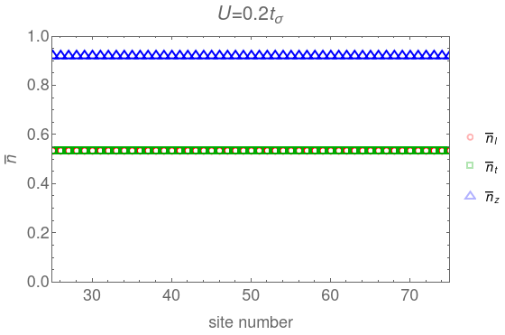
(b)

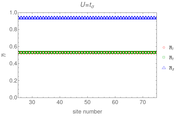
Figure 8: Site-dependent ground state orbital occupations $\{\bar{n}_{\mu}\}$ in the local basis as obtained from DMRG calculations of the Hubbard model (1) on an $L=100$-site chain with: $\text{(a)}\;U=0.2\;t_{\sigma}$,   (b) $U=t_{\sigma}$. Open boundary conditions are imposed and only densities on the ‘middle’ 50 sites of the chain are shown.

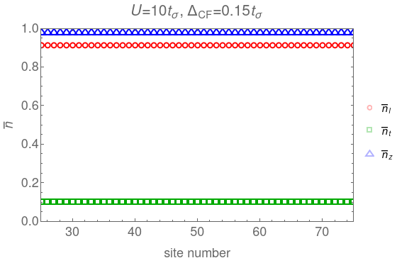
Figure 9: Site-dependent ground state orbital occupations $\{\bar{n}_{\mu}\}$ in the local basis as obtained from DMRG calculations of the Hubbard model (1) with $U=10t_{\sigma}$ and with crystal field $\Delta_{\rm CF}=0.15\;t_{\sigma}$ on an $L=100$-site chain (see text for further details). Open boundary conditions are imposed and only densities on the ‘middle’ 50 sites of the chain are shown.

In order to test the accuracy of the Hartree approximation (see main text), we performed preliminary DMRG calculations [29] on systems of size $L\times 3$, $L$ being the number of sites in the chain and 3 being the number of orbitals per site. We use open boundary conditions. We fix $L=100$ in our calculations and keep up to $m=2000$ density-matrix eigenvalues in the renormalization procedure. This way we are able to obtain accurate results with an error $\delta/L=10^{-10}$. To suppress the edge effects, in what follows we plot the local orbital densities for all sites between site number $L/4$ and site number $3L/4$ in the chain.

B.1 Weak Coupling

In the weak coupling regime, extending to at least $U=t_{\sigma}$, we find that the DMRG results and the Hartree approximation results (see main text) are in perfect agreement, see Fig 8. This is due to the fact that the non-interacting system is in an orbitally-ordered phase protected by a finite energy gap, so that the (quantum) fluctuations in orbital densities are indeed negligible.

B.2 Strong Coupling

In the strong coupling regime we find that a small but finite symmetry-breaking crystal field $\Delta_{\rm CF}$ term must be included in the DMRG calculations to stabilise the ‘2-2-0’ orbital density wave predicted by the Hartree approximation, see Fig. 9. Note that such a field, which raises the on-site energy of one of the orbitals in the bond-angle plane (e.g. the $p_{t}$ orbital as assumed here), may possibly arise in a model for a single chiral chain of the 3D chalcogen crystal once the influence of the neighboring chains (as arising from the electron tunneling or Coulomb interactions) is taken into account. This is because, for bond angles greater than 90^∘, the presence of the neighboring chains needs to affect the on-site energies of the two orbitals lying in the bond angle plane differently [since one of them is oriented more along the chain ($p_{l}$)].

Without such a finite symmetry-breaking term the ‘2-2-0’ orbital density wave predicted by the Hartree approximation (see main text) is not recovered in our preliminary DMRG calculations for the Hubbard model with $U=10\;t_{\sigma}$. In fact, the calculation fails due to very long convergence time. To comment on this a little further, let us note that if one considers the extremely correlated regime ($U=20\;t_{\sigma}$) the calculation converges (unshown). In this case the result with zero crystal-field exhibits strong orbital density fluctuations in real space. We expect this to be—at least partially—the effect of the open edges. Importantly, in this extremely correlated regime we find a 50-fold increase in the CPU time for the calculation without the symmetry breaking field w.r.t. the calculation with the symmetry-breaking field included or the calculation for the weak coupling case ($U\leq t_{\sigma}$). This suggests the presence of competing interactions in the system and means that large-scale, state-of-the-art numerics are needed to establish the exact nature of the ground state without symmetry breaking field, possible order in the strong coupling limit or the dependence of the results on boundary conditions.

References

- Hirsch [1984] J. E. Hirsch, “Charge-density-wave to spin-density-wave transition in the extended Hubbard model,” Phys. Rev. Lett. 53, 2327–2330 (1984).
- van Dongen [1994] P. G. J. van Dongen, “Extended Hubbard model at strong coupling,” Phys. Rev. B 49, 7904–7915 (1994).
- Tsuchiizu and Furusaki [2002] M. Tsuchiizu and A. Furusaki, “Phase diagram of the one-dimensional extended Hubbard model at half filling,” Phys. Rev. Lett. 88, 056402 (2002).
- Goodenough [1955] J. B. Goodenough, “Theory of the role of covalence in the perovskite-type manganites [La, M(II)]MnO3,” Phys. Rev. 100, 564 (1955).
- van Wezel [2011] J. van Wezel, “Chirality and orbital order in charge density waves,” EPL (Europhysics Letters) 96, 67011 (2011).
- van Wezel [2012] J. van Wezel, “Polar charge and orbital order in 2H-TaS2,” Phys. Rev. B 85, 035131 (2012).
- Fukutome [1984] H. Fukutome, “Charge density wave-soliton model for Se and Te,” Prog. Theor. Phys. 71, 1–15 (1984).
- Shimoi and Fukutome [1992] Y. Shimoi and H. Fukutome, “Vector charge density wave model of metallic and trigonal Te,” Prog. Theor. Phys. 87, 307–329 (1992).
- van Wezel and Littlewood [2010] J. van Wezel and P. Littlewood, “Chiral symmetry breaking and charge order,” Physics 3, 87 (2010).
- Silva et al. [2018] Ana Silva, J. Henke, and J. van Wezel, “Elemental chalcogens as a minimal model for combined charge and orbital order,” Phys. Rev. B 97, 045151 (2018).
- Von Hippel [1948] A. Von Hippel, “Structure and conductivity in the VI b group of the periodic system,” The Journal of Chemical Physics 16, 372–380 (1948).
- Reitz [1957] J. R. Reitz, “Electronic band structure of selenium and tellurium,” Phys. Rev. 105, 1233–1240 (1957).
- Tanaka et al. [2010] Y. Tanaka, S. P. Collins, S. W. Lovesey, M. Matsumami, T. Moriwaki, and S. Shin, “Determination of the absolute chirality of tellurium using resonant diffraction with circularly polarized x-rays,” J. Phys.: Condens. Matter , 122201 (2010).
- Demirci et al. [2020] S. Demirci, H. H. Gurel, S. Johangirov, and S. Ciraci, “Temperature, strain and charge mediated multiple and dynamical phase changes of selenium and tellurium,” Nanoscale 12, 3249–3258 (2020).
- Akahama et al. [1992] Y. Akahama, M. Kobayashi, and H. Kawamura, “Pressure-induced superconductivity and phase transition in selenium and tellurium,” Solid State Communications 84, 803 – 806 (1992).
- Struzhkin et al. [1997] V. V. Struzhkin, R. J. Hemley, H.-K. Mao, and Y. A. Timofeev, “Superconductivity at 10–17 K in compressed sulphur,” Nature 390, 382–384 (1997).
- Matsui [2014] M. Matsui, “Role of interchain interaction in determining the band gap of trigonal selenium: A density functional theory study with a linear combination of Bloch orbitals,” The Journal of Physical Chemistry C 118, 19294–19307 (2014).
- Silva and van Wezel [2018] Ana Silva and J. van Wezel, “The simple-cubic structure of elemental Polonium and its relation to combined charge and orbital order in other elemental chalcogens,” SciPost Phys. 4, 028 (2018).
- Olechna and Knox [1965] D. J. Olechna and R. S. Knox, “Energy-band structure of selenium chains,” Phys. Rev. 140, A986–A993 (1965).
- Chen and Das [1966] I. Chen and T. P. Das, “Molecular orbital theory of sulfur and selenium radicals,” The Journal of Chemical Physics 45, 3526–3535 (1966).
- Tutihasi and Chen [1967] S. Tutihasi and I. Chen, “Optical properties and band structure of trigonal selenium,” Phys. Rev. 158, 623–630 (1967).
- Cherin and Unger [1967] P. Cherin and P. Unger, “The crystal structure of trigonal selenium,” Inorganic Chemistry 6, 1589–1591 (1967).
- Slater and Koster [1954] J. C. Slater and G. F. Koster, “Simplified LCAO method for the periodic potential problem,” Phys. Rev. 94, 1498–1524 (1954).
- Oleś [1983] A. M. Oleś, “Antiferromagnetism and correlation of electrons in transition metals,” Phys. Rev. B 28, 327–339 (1983).
- Zhang [2014] Qian Zhang, Calculations of atomic multiplets across the periodic table, Ms, RWTH Aachen (2014), RWTH Aachen, Masterarbeit, 2014.
- Deng et al. [2007] S. Deng, A. Simon, and J. Köhler, “Lone pairs, bipolarons and superconductivity in tellurium,” in High Superconductors and Related Transition Metal Oxides: Special Contributions in Honor of K. Alex Müller on the Occasion of his 80th Birthday, edited by Annette Bussmann-Holder and Hugo Keller (Springer Berlin Heidelberg, Berlin, Heidelberg, 2007) pp. 201–211.
- Deng et al. [2006] S. Deng, J. Köhler, and A. Simon, “Unusual lone pairs in tellurium and their relevance for superconductivity,” Angewandte Chemie International Edition 45, 599–602 (2006).
- Khomskii [2014] Daniel I. Khomskii, Transition Metal Compounds (Cambridge University Press, 2014).
- White [1993] Steven R. White, “Density-matrix algorithms for quantum renormalization groups,” Phys. Rev. B 48, 10345–10356 (1993).