Modulated rotating waves and triadic resonances in spherical fluid systems: The case of magnetized spherical Couette flow

Abstract

The existence of triadic resonances in the magnetized spherical Couette system (MSC) is related to the development of modulated rotating waves, which are quasiperiodic flows understood in terms of bifurcation theory in systems with symmetry. In contrast to previous studies in spherical geometry the resonant modes are not inertial waves but related with the radial jet instability which is strongly equatorially antisymmetric. We propose a general framework in which triadic resonances are generated through successive Hopf bifurcations from the base state. The study relies on an accurate frequency analysis of different modes of the flow, for solutions belonging to two different bifurcation scenarios. The azimuthal and latitudinal nonlinear coupling among the resonant modes is analysed and interpreted using spherical harmonics and the results are compared with previous studies in spherical geometry.

I Introduction

The onset of instabilites in rotating fluids is often related to the emergence of a triadic resonance, which describes a resonant interaction between three internal modes or waves that requires the fulfillment of certain selection rules in order to take place. Such interactions occur on a small scales in the laboratory as well as on large scales in geo- or astrophysically relevant fluid flows. In the case of ocean flows, for example, the relevance of weak wave resonant interactions for the global wave evolution has been investigated for several decades (e. g. Hammack and Henderson (1993)). More recent examples comprise the study of internal tides models of Sutherland and Jefferson (2020), the experiments on gravity surface turbulence of Campagne et al. (2019), or the theoretical study of Li et al. (2020) devoted to the analysis of steady state resonant interfacial waves in a two layer fluid filling a duct.

Regarding celestial bodies, rotating (and electrically conducting) fluids are responsible for the generation of magnetic fields (Jones (2011)). These flows are assumed to be turbulent which raises the question of the initial instabilities and the related weakly nonlinear interactions (e. g. Le Bars, Cébron, and Le Gal (2015)). It is well known that resonant interactions are responsible for energy transfers among different modes (e. g. Waleffe (1992); Smith and Waleffe (1999); Galtier (2003)). Recent experiments of Brunet, Gallet, and Cortet (2020) on wave-driven rotating turbulence have shown the existence of a secondary instability involving four resonant waves that feed an unforced geostrophic flow.

The triadic instabilites found in simulations and experiments of precessing cylinders (Lagrange, Nadal, and Eloy (2011); Herault et al. (2015); Giesecke et al. (2015)) have been linked to Hopf bifurcations from the steady base state that goes along with the transition from regular (periodic and quasiperiodic) flows to chaotic flows (Albrecht et al. (2015); Lopez and Marques (2018)).

Recently, triadic resonances were also identified in spherical systems (e. g. Hoff, Harlander, and Triana (2016); Barik et al. (2018); Lin (2021)). In the case of mechanically driven Couette flow in a wide-gap spherical shell, Barik et al. (2018) discussed the appearance of a triadic resonance regime in which free inertial modes form a triad with the basic non-axisymmetric instability. For convection driven fluid flows in full spheres a triadic resonance regime involving inertial waves was found in Lin (2021) linking convection and mechanical drivings in agreement with the theoretical analysis of Zhang and Liao (2017) performed in terms of inertial waves and for either convective or mechanically forced rotating fluids systems.

Inertial waves are solutions of the inviscid Navier-Stokes equations for which the Coriolis effects are dominant (e. g. Greenspan (1968); Rieutord and Valdettaro (1997); Zhang et al. (2001)). In the context of the spherical Couette flow inertial wave-like motions were identified in the experimental study of Kelley et al. (2007), which provided evidence of the generation of these type of motions when the flow is driven by strong differential rotation. For the same problem, the study of Barik et al. (2018) showed that at higher rotation rates the fundamental instability is a shear-layer instability (Stewartson (1966); Hollerbach et al. (2004)), equatorially symmetric and nearly geostrophic, which forms a triad with two equatorially antisymmetric inertial modes. This instability emerges when Coriolis forces prevail (as required for inertial geostrophic columns, see Wicht (2014)).

We demonstrate that the weakly nonlinear solutions of the magnetized spherical Couette system (MSC) satisfy triadic resonance interactions that involve different azimuthal and latitudinal modes. These modes are not inertial waves but related to the radial jet instability (Hollerbach, Junk, and Egbers (2006); Garcia and Stefani (2018); Garcia et al. (2019, 2020b)), which is basically hydrodynamic because the effects of the applied magnetic field are weak. Contrasting to the results of Barik et al. (2018) the radial jet instability develops when viscous, rather than Coriolis, forces are dominant. Triadic resonant flows emerge from the base state via a sequence of Hopf bifurcations similar to the scenario described in Albrecht et al. (2015) and Lopez and Marques (2018) for the precessing cylinder. We show that this link between triadic instability and Hopf bifurcations to periodic and quasiperiodic flows is then valid as well in spherical geometry using the particular example of the MSC system. The sequence of bifurcations is obtained by modifying the magnetic field strength, though similar bifurcations are expected when the magnitude of imposed differential rotation is increased (Hollerbach (2009); Travnikov, Eckert, and Odenbach (2011)).

Concretely, the quasiperiodic solutions having resonant modes are modulated rotating waves (MRW), for which a developed theory in terms of equivariant dynamical systems exists (Rand (1982); Crawford and Knobloch (1991); Coughlin and Marcus (1992); Golubitsky, LeBlanc, and Melbourne (2000); Golubitsky and Stewart (2003)). These solutions have certain spatio-temporal symmetries and appear since the system is SO$(2)\times$Z₂-equivariant, i. e., invariant by azimuthal rotations and reflections with respect to the equatorial plane. We show that an instability in terms of a triadic resonance consisting of three resonantly interacting modes can equivalently be described in terms of a MRW. The spatio-temporal symmetry of the MRWs renders possible the existence of triadic resonant relations among several modes which reflect the quadratic nature of the nonlinear interaction.

While the mechanism proposed here is more general, it is not in contradiction with the interpretation of triadic resonances in terms of inertial waves, as quasiperiodic MRW involving inertial modes can be found as well in spherical (e. g. Garcia, Chambers, and Watts (2019); Lin (2021)) and cylindrical geometry (e. g. Albrecht et al. (2018)), and their mathematical description is analogous to that of inertial waves of Barik et al. (2018) and the references therein. We demonstrate that resonant interactions prevail on a significant region of the parameter space and even for chaotic flows, generated from further bifurcations of quasiperiodic MRW.

The organization of the paper is the following: In § II the model problem is introduced and the numerical method used is briefly described. In § III we argue how triadic resonances develop for MRWs considering the azimuthal dependence. The identification and description of resonant triads for two different scenarios and the comparison with previous studies is completed in § IV while the latitudinal dependence among the resonant modes is discussed in § V. The paper closes with § VI, summarizing the results obtained.

II The model equations

The magnetized spherical Couette system consist of an electrically conducting fluid of density $\rho$, kinematic viscosity $\nu$, magnetic diffusivity $\eta=1/(\sigma\mu_{0})$ (where $\mu_{0}$ is the magnetic permeability of the free-space and $\sigma$ is the electrical conductivity), which fills the space between two spheres with radius $r_{\text{i}}$ and $r_{\text{o}}$, respectively. The gap width selected for this study is $\chi=r_{\text{i}}/r_{\text{o}}=0.5$. The outer sphere is at rest and the inner sphere is rotating at angular velocity $\Omega$ around the vertical axis ${\bf\hat{e}_{z}}$, and a uniform axial magnetic field of amplitude $B_{0}$ is applied. This model has been successfully employed to compare with the very recent experiments of Ogbonna et al. (2020) in which a liquid metal within a differentially rotating spherical vessel is subjected to an axial magnetic field. In these experiments RWs of azimuthal symmetries $m\in\{2,3,4\}$ were found in the return flow instability regime for ${\rm Re}=10^{3}$ and ${\rm Ha}\in[27.5,40]$.

The system is described by the Navier-Stokes and induction equations scaling the length, time, velocity and magnetic field with $d=r_{\text{o}}-r_{\text{i}}$, $d^{2}/\nu$, $r_{\text{i}}\Omega$ and $B_{0}$, respectively. The time dependent equations are:

$$\partial_{t}{\mathbf{v}}+{\rm Re}\left({\mathbf{v}}\cdot\nabla\right){\mathbf{v}}=-\nabla p+\nabla^{2}{\mathbf{v}}+{\rm Ha}^{2}(\nabla\times{\bf b})\times{\bf\hat{e}_{z}},$$ (1)

$$0=\nabla\times({\mathbf{v}}\times{\bf\hat{e}_{z}})+\nabla^{2}{\bf b},\quad\nabla\cdot{\mathbf{v}}=0,\quad\nabla\cdot{\bf b}=0,$$ (2)

where ${\rm Re}=\Omega r_{\text{i}}d/\nu$ is the Reynolds number, ${\rm Ha}=B_{0}d(\sigma/(\rho\nu))^{1/2}$ is the Hartmann number, ${\mathbf{v}}$ the velocity field and ${\bf b}$ the deviation of the magnetic field from the axial applied field.

The inductionless approximation is used since it is valid in the limit of small magnetic Reynolds number, ${\rm Rm}=\Omega r_{\text{i}}d/\eta\ll 1$. This is the case for the liquid metal considered, GaInSn, with magnetic Prandtl number ${\rm Pm}=\nu/\eta\sim O(10^{-6})$ (Plevachuk et al. (2014)), at moderate ${\rm Re}=10^{3}$, since ${\rm Rm}={\rm Pm}\hskip 1.42262pt{\rm Re}\sim 10^{-3}$. The boundary conditions for the velocity field are no-slip ($v_{r}=v_{\theta}=v_{\varphi}=0$) at $r=r_{\text{o}}$ and constant rotation ($v_{r}=v_{\theta}=0,~{}v_{\varphi}=\sin{\theta}$, $r$, $\theta$ and $\varphi$ being the radius, colatitude and longitude, respectively) at $r=r_{\text{i}}$. For the magnetic field insulating boundary conditions are applied in accordance with the experimental setups (Sisan et al. (2004); Ogbonna et al. (2020)).

To solve the model equations the toroidal-poloidal formulation (Chandrasekhar (1981)), in which the velocity field is expressed in terms of toroidal, $\Psi$, and poloidal, $\Phi$, potentials

$${\mathbf{v}}=\nabla\times\left(\Psi\mathbf{r}\right)+\nabla\times\nabla\times\left(\Phi\mathbf{r}\right),$$ (3)

is used. The potentials are expressed in terms of the spherical harmonics angular functions (truncated at order and degree $m=l=L_{\text{max}}$) and in the radial direction a collocation method on a Gauss–Lobatto mesh of $N_{r}$ points is employed. The toroidal ($\Psi$) and poloidal ($\Phi$) potentials are then

$$\Psi(t,r,\theta,\varphi)=\sum_{l=0}^{L_{\text{max}}}\sum_{m=-l}^{l}{\Psi_{l}^{m}(r,t)Y_{l}^{m}(\theta,\varphi)},$$ (4)

$$\Phi(t,r,\theta,\varphi)=\sum_{l=0}^{L_{\text{max}}}\sum_{m=-l}^{l}{\Phi_{l}^{m}(r,t)Y_{l}^{m}(\theta,\varphi)},$$ (5)

with $\Psi_{l}^{-m}=\overline{\Psi_{l}^{m}}$, $\Phi_{l}^{-m}=\overline{\Phi_{l}^{m}}$, $\Psi_{0}^{0}=\Phi_{0}^{0}=0$ to uniquely determine the two potentials, and $Y_{l}^{m}(\theta,\varphi)=P_{l}^{m}(\cos\theta)e^{im\varphi}$, $P_{l}^{m}$ being the normalized associated Legendre functions of degree $l$ and order $m$. The code is parallelized in the spectral and in the physical space by using OpenMP directives. We use optimized libraries (FFTW3 Frigo and Johnson (2005)) for the FFTs in $\varphi$ and matrix-matrix products (dgemm GOTO Goto and van de Geijn (2008)) for the Legendre transforms in $\theta$ when computing the nonlinear terms (see Garcia et al. (2010) for further details).

The time integration is based on high order implicit-explicit backward differentiation formulas (IMEX–BDF) fully described in Garcia et al. (2010). The nonlinear terms are treated explicitly to avoid the implicit solution of nonlinear systems. To simplify the resolution of linear systems, the Lorenz term is also treated explicitly. This may lead to reduced time steps in comparison with an implicit treatment if large ${\rm Ha}$ numbers are considered, which however is not the case of the present study with ${\rm Ha}\sim O(1)$.

III Triadic resonances

The conditions for triadic resonances among inertial modes were established in Barik et al. (2018) (see their sections 2 and 7, and appendix A). Expanding the velocity and pressure fields in terms of the Rossby number the zeroth order of the Navier-Stokes equations leads to the inertial mode equation, with the resonant modes being of the form $u_{i}(t,r,\theta,\varphi)=c_{i}(t,r,\theta)\text{e}^{i(m_{i}\varphi-\omega_{i}t)}$, $i=1,2$. The subsequent analysis of the first order equation provides the resonance conditions, which are obtained by computing the quadratic advection term of the sum $u_{1}+u_{2}$ (assumed to be an approximation of the zeroth-order solution).

The time dependence of a rotating wave (RW) is described by a solid body rotation of a fixed spatial pattern with a certain rotation frequency $\omega$. Because of this, they are steady flows if the change of variables $\overline{\varphi}=\varphi+\omega t$ is applied to the Navier-Stokes equations (Eqs. (1)-(2)), see Rand (1982); Sánchez, Garcia, and Net (2013); Garcia, Net, and Sánchez (2016); Garcia et al. (2019) for a theoretical description and applications of RWs in spherical systems. If the azimuthal symmetry of the RW is $m_{0}$ , the spherical harmonic amplitudes of the toroidal and poloidal potentials (Eqs. (4)-(5)) become

$$\Psi_{l}^{m_{0}k}(r,t)=\overline{\Psi}_{l}^{m_{0}k}(r)~{}e^{-im_{0}k\omega t},$$

$$\Phi_{l}^{m_{0}k}(r,t)=\overline{\Phi}_{l}^{m_{0}k}(r)~{}e^{-im_{0}k\omega t},$$

with $k\in\mathbb{Z}$. This is the same expression as given in Eq. (A5a,b) of Barik et al. (2018) for the inertial modes, restricted to $m=km_{0}$. The relation between their values of the frequencies ($\omega_{j}$) of each inertial mode and the rotation frequency of the RW waves is $\omega_{j}=j\omega$. The above expressions for the spherical harmonic amplitudes of the potentials evidence that RWs fulfil the trivial triadic resonance conditions

$$(i\pm j)m_{0}=im_{0}\pm jm_{0},\quad\omega_{i\pm j}=\omega_{i}\pm\omega_{j}=(i\pm j)\omega.$$ (6)

Usually RW give rise to MRW by means of Hopf-type bifurcations (see for instance Rand (1982); Sánchez, Garcia, and Net (2013); Garcia, Net, and Sánchez (2016); Garcia et al. (2019)). We now argue how triadic resonances can be described in terms of RWs and MRWs. Close to the bifurcation point a MRW can be approximated by $u_{0}+\epsilon\delta u_{0}$ where $u_{0}$ is a RW and $\delta u_{0}$ the corresponding perturbation (Floquet eigenmode, since RW are periodic orbits, see for instance Kuznetsov (1998); Sánchez and Net (2016); Garcia and Stefani (2018)). For the sake of simplicity only the azimuthal dependence is considered in the following and the investigation about the role of the latitude is reserved to § V. Consider a RW with azimuthal symmetry $m_{0}$ and rotation frequency $\omega$ having the energy mainly contained in the $m_{0}$ mode so it can be approximated by $u_{o}(t,\varphi)=u_{m_{o}}\text{e}^{im_{0}(\varphi-\omega t)}$. We approximate now the perturbation as $\delta u_{0}(t,\varphi)=\overline{u}_{m_{1}}(t)\text{e}^{im_{1}\varphi}=u_{m_{1}}(t)\text{e}^{i(m_{1}\varphi-\omega_{1}t)}$ where $\omega_{1}$ is the new frequency provided by the Hopf bifurcation and $m_{1}$ is the azimuthal symmetry of the Floquet mode (see Garcia et al. (2019) for details). The quadratic terms $u_{o}\delta u_{0}$ appearing in the advection term of the Navier-Stokes equations will then exite a resonant mode since

$$\text{e}^{im_{0}(\varphi-\omega t)}\cdot\text{e}^{i(m_{1}\varphi-\omega_{1}t)}=\text{e}^{i((m_{0}+m_{1})\varphi-(m_{0}\omega+\omega_{1})t)}.$$ (7)

The triadic resonance conditions will be then

$$\omega_{2} = \omega_{0}+\omega_{1},\quad\text{with}\quad\omega_{0}=m_{0}\omega$$

$$m_{2} = m_{0}+m_{1}.$$

We note that as MRW are quasiperiodic, the frequencies $\omega_{0}$ and $\omega_{1}$ are generically incommensurable so MRW can be mathematically expressed like solutions of the inertial equation as in Eq. (A5a,b) of Barik et al. (2018). The only condition is that the axisymmetry of the base state needs to be broken by means of a Hopf bifurcation (Ecke, Zhong, and Knobloch (1992); Crawford and Knobloch (1991)). We also remark that if $m_{1}=m_{0}$ the nonlinear interactions of Eq. (7) are added to the self nonlinear interactions of $u_{0}$, so the trivial resonance conditions given in Eq. (6) may prevail.

IV Results

In this section we investigate triadic resonances involving different spherical harmonic degree $m$ and order $l$ for a set of several RW and MRW belonging to two different scenarios already studied in Garcia et al. (2019, 2020b). The parameters selected for the study are an aspect ratio $\chi=0.5$, a Reynolds number ${\rm Re}=10^{3}$, and several Hartmann numbers with ${\rm Ha}<12.2$. For these parameters the first instability for the steady axisymmetric base flow is nonaxisymmetric with $m=3$ azimuthal symmetry, and antisymmetric with respect to the equator (Travnikov, Eckert, and Odenbach (2011)). This instability is usually called “radial jet” since a strong jet flowing outwards from the inner sphere at equatorial latitudes is developed (Hollerbach, Junk, and Egbers (2006)).

The first bifurcated nonlinear RWs, either stable or unstable with azimuthal symmetries $m\in{2,3,4}$, were computed by Garcia and Stefani (2018) where the dependence of the associated rotation frequencies $\omega$ on $Ha$ on was described. In the following we investigate resonances among different modes that constitute a MRW. We consider several MRWs that bifurcate from the different branches of RWs with azimuthal symmetry $m=3$ and $m=4$ (see Garcia and Stefani (2018), Garcia et al. (2019), and Garcia et al. (2020b) for further details of these MRWs).

Two different bifurcation scenarios with increasing complexity and different sequences of azimuthal symmetry breakings are selected to strengthen the link between different types MRW and triadic resonances. Because MRW are quasiperiodic flows (invariant tori) they are classified according to the number (two, three or four) of incommensurable frequencies as 2T, 3T or 4T (“T” standing for Tori). The first bifurcation scenario provides the usual description of stable flows (RWs and MRWs) emerging from an axisymmetric base state. In this case the sequence of azimuthal symmetries of the flow is: $m=0$ (base state), $m=3$ (RWs), and $m=1$ (2T and 3T MRWs). For the second scenario, a larger number of bifurcations are analyzed. In this case the sequence of azimuthal symmetries is: $m=0$ (base state), $m=4$ (unstable RWs and 2T MRW), $m=2$ (3T MRWs), and $m=1$ (4T MRWs and chaotic flows). Considering this second scenario allows us to demonstrate the occurrence of triadic resonances even for chaotic flows.

Each solution has been obtained using direct numerical simulations of Eqs. (1-2), from which the initial transients are discarded. The spherical harmonics series of the fields (Eqs. (4) and (5)) have been truncated at an order and degree of $L_{\text{max}}=84$, and $N_{r}=40$ inner collocation points are used in the radial direction. The computations have been already validated in Garcia and Stefani (2018); Garcia et al. (2020b) by increasing $L_{\text{max}}$ and $N_{r}$ up to $126$ and $60$, respectively. To detect resonant modes we analyse time series obtained from the poloidal potential $\Phi$ since it is directly related with the radial velocity component

$$v_{r} =-\frac{1}{r\sin\theta}\left(\sin\theta\partial^{2}_{\theta\theta}\Phi+\cos\theta\partial_{\theta}\Phi+\frac{1}{\sin\theta}\partial^{2}_{\varphi\varphi}\Phi\right).$$

The radial velocity component naturally reflects the structure of the instabilities as it measures the jet outwards velocity at equatorial latitudes and it is related with the meridional circulation developed at larger latitudes.

IV.1 Identification of triadic resonances

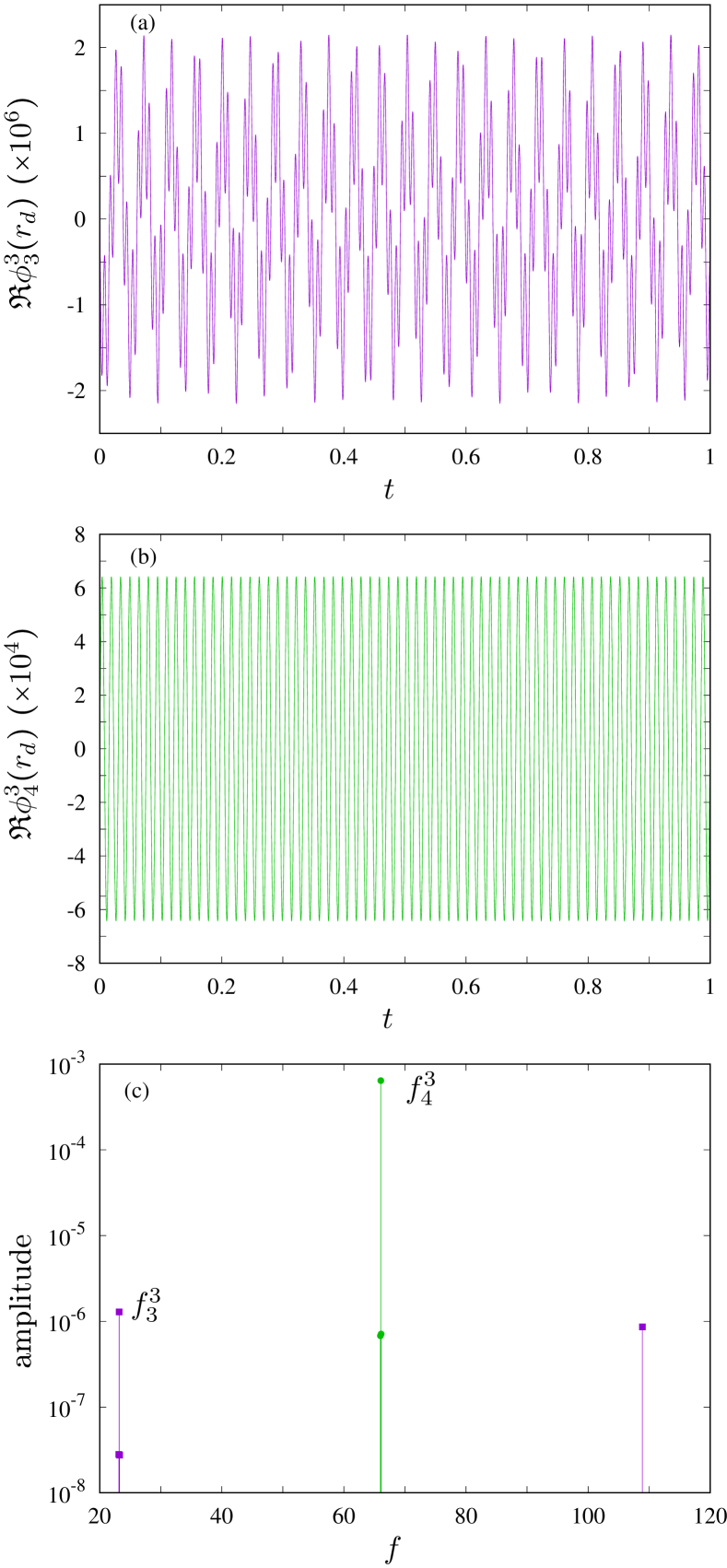
Figure 1: (a) The time series of $\Re{\Phi^{3}_{3}(r_{d})}$ is modulated. (b) The time series for $\Re{\Phi^{3}_{4}(r_{d})}$ is periodic. (c) The first four frequencies of largest amplitude from the frequency spectrum of $\Re{\Phi^{3}_{3}(r_{d})}$ (squares) and of $\Re{\Phi^{3}_{4}(r_{d})}$ (circles). The peaks selected for the resonance relations shown in table 1 are labelled on the plot. The time series in (a) and (b) is obtained for the 2T MRW solution at ${\rm Ha}=3.5$ which has $m=1$ azimuthal symmetry.

For analyzing the frequency spectrum it is sufficient to consider either the poloidal or the toroidal components, since both components reflect the same frequencies in case of regular flows (see e.g. Fig. 4a in Barik et al. (2018)). Because of the symmetry, the time series of any equatorially symmetric (resp. antisymmetric) poloidal mode, at a given radius, will exhibit the same main peak in their frequency spectrum. That means that for each $m$ we incorporate the poloidal mode with $l=m$ (i. e. $\Phi_{m}^{m}$ which corresponds to an equatorially symmetric term) and the poloidal mode with $l=m+1$ (i.e. $\Phi_{m+1}^{m}$ which corresponds to an equatorially antisymmetric term) . In order to identify triadic resonances, we specifically consider the time series of the real part of the poloidal amplitude $R\Phi_{l}^{m}(r_{d})$, where $r_{d}=(r_{i}+r_{o})/2$ is the middle shell radius, for several azimuthal wave numbers $m\in{1,...,12}$ and spherical harmonic degrees $l\in{1,...,13}$.

We compute the frequency spectrum of each time series by means of Laskar’s algorithm (Laskar (1990); Laskar, Froeschlé, and Celletti (1992); Laskar (1993)), implemented in the SDDSToolkit (Borland et al. (2017)), which is an accurate method for the determination of the fundamental frequencies of a time series up to prescribed tolerance. We select the frequency among the four peaks having largest amplitude in the way we now describe. The first peak is selected when its amplitude is significantly larger than the others. When there are several peaks of similar magnitude, we select the frequency which provides the larger number of resonance conditions, which is usually the largest peak. Figure 1 exemplifies this procedure by displaying two examples of time series and the corresponding frequency analysis for the modes $(m,l)\in\{(3,3),(3,4)\}$. The time series originates from the 2T MRW with azimuthal symmetry $m=1$ at ${\rm Ha}=3.5$ first studied in Garcia et al. (2019). The time series of $R\Phi_{3}^{3}(r_{d})$ (panel (a)) is clearly quasiperiodic with the corresponding frequency spectrum displaying two peaks of similar magnitude (panel (c), squares) whereas the time series of $R\Phi_{4}^{3}(r_{d})$ (panel (b)) is periodic with one single strong peak in the spectrum (panel (c), circles).

When the frequency $f^{m}_{l}$ corresponding to each mode $(m,l)$ is available, we seek for triadic resonances defined as

$$f^{m_{0}}_{l_{0}}=f^{m_{1}}_{l_{1}}+f^{m_{2}}_{l_{2}},\quad m_{0}=m_{1}+m_{2},$$ (8)

for $m_{i}\in\{1,...,11\}$. The relative errors

$$\epsilon_{f}=(f^{m_{0}}_{l_{0}}-f^{m_{1}}_{l_{1}}-f^{m_{2}}_{l_{2}})/f^{m_{0}}_{l_{0}}$$

are computed for all the combinations satisfying $m_{0}=m_{1}+m_{2}$, and $l_{i}=m_{i}$ or $l_{i}=m_{i}+1$ ($i=0,1,2$), with $m_{0}=3,....,12$. We assume a resonance condition when the relative error is sufficiently small, namely, $\epsilon_{f}<10^{-4}$. This value is similar to the accuracy obtained for the determination of the fundamental frequency suggested by the numerical experiments of Garcia et al. (2021) performed in the same parameter region as in the present study.

We note that there are resonances for which $l_{0}=l_{1}+l_{2}$ holds as well, so the spherical harmonic degrees $l_{i}$ fulfill a similar condition as the azimuthal wave numbers. In these cases the latitudinal structure imposes an additional constraint for the emergence of a triadic resonance. Note that for fixed $(m_{i},l_{i})$, $i=0,1,2$, obeying the condition (8), the condition $f^{m_{0}}_{l_{0}}=f^{m_{1}}_{l_{1}+2k}+f^{m_{2}}_{l_{2}+2k}$, $k=1,2,..$ holds as well since for modes $(m_{i},l_{i}+2k)$ and $(m_{i},l_{i})$ have the same frequency, as they have the same azimuthal wave number and equatorial symmetry. But even if the condition $l_{0}=l_{1}+l_{2}$ is not strictly fulfilled, the resonance relations given in Eq. (8) have to respect the equatorial symmetry, in the sense that $l_{0}$ and $l_{1}+l_{2}$ must have the same parity.

To check that the triad interactions preserve the same phase relation during the whole time series a statistical measure, the bicoherence, was estimated in Barik et al. (2018); Hoff, Harlander, and Triana (2016). In our study this is checked by directly computing the phase $\xi^{m}_{l}$ associated to the frequencies $f^{m}_{l}$ of the interacting modes $(m,l)$, which can be easily done with Laskar’s algorithm. The phase is computed on a specific time window of length $T<T_{f}$, $T_{f}$ being the total length of the time series, which is varied to obtain a time dependent value of the phase, and also of the corresponding frequency (e. g. Garcia et al. (2021)). For each resonance relation like Eq. (8) the corresponding time dependent phases $\xi^{m}_{l}(t)$ must satisfy

$$\xi^{m_{0}}_{l_{0}}(t)=\xi^{m_{1}}_{l_{1}}(t)+\xi^{m_{2}}_{l_{2}}(t),\quad m_{0}=m_{1}+m_{2},$$ (9)

up to a given tolerance.

IV.2 Path to triadic resonances from the base state

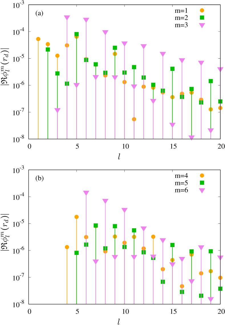
Figure 2: Snapshot of the poloidal amplitudes $|\Re{\Phi^{m}_{l}(r_{d})}|$, where $r_{d}=(r_{i}+r_{o})/2$, versus the degree $l$ for $m\in\{1,..,6\}$. The solution is a modulated rotating wave with $m=1$ azimuthal symmetry at ${\rm Ha}=3.5$.

This subsection details the investigation of the development of triadic resonances among spherical harmonic modes of nonlinear solutions bifurcating directly from the steady axisymmetric base state. At $\chi=0.5$ and ${\rm Re}=10^{3}$ the onset of a nonaxisymmetric radial jet instability is at ${\rm Ha}_{c}=12.2$, a value determined in Travnikov, Eckert, and Odenbach (2011) from a linear stability analysis. The linear instability takes the form of an equatorially antisymmetric radial jet with azimuthal symmetry $m=3$ and thus equatorially asymmetric nonlinear rotating waves with azimuthal symmetry $m=3$ are the first time dependent flows (e. g. Ecke, Zhong, and Knobloch (1992); Garcia and Stefani (2018)). The spherical harmonic amplitudes for the poloidal field (Eq. (5)) are given by

$$\Phi_{l}^{3k}(r,t)=\overline{\Phi}_{l}^{3k}(r)~{}e^{-i3k\omega t},$$ (10)

with $\omega$ being the rotation frequency of the wave and $\overline{\Phi}_{l}^{3k}(r)$ a function which only depends on the radial coordinate (see § III). We note that these RW have in addition a more particular structure since $\overline{\Phi}_{l}^{3k}(r)=0$ when $l$ is odd. This means that the mode $m=3k$ is equatorially symmetric (resp. antisymmetric) if $k$ is even (resp. odd). Because $f^{m}_{l}=m\omega/2\pi$ these RWs satisfy the trivial triadic resonance conditions

$$f^{3}_{4}=f^{9}_{10}-f^{6}_{6}=f^{12}_{12}-f^{9}_{10}=f^{15}_{16}-f^{12}_{12}=...,$$

where the frequencies $f^{m}_{l}$ correspond to those of largest PSD of the time series of $\Re{\Phi^{m}_{l}(r_{d})}$. We note that for each azimuthal mode $m=3k$, $k=1,2,...$, there is a latitudinal mode $l$ which verifies the resonance condition as well. For instance the relation $f^{3}_{4}=f^{12}_{12}-f^{9}_{10}$ of above is equivalent to $f^{3}_{4}=f^{12}_{14}-f^{9}_{10}$ since $f^{12}_{14}=f^{12}_{12}$.

Table 1: Relations between the main frequencies $f^{m}_{l}$ of the different modes $(m,l)$ for the 2T MRW with $m=1$ azimuthal symmetry at ${\rm Ha}=3.5$ and the 3T MRW with $m=1$ azimuthal symmetry at ${\rm Ha}=3.10$. These relations are satisfied up to $(f^{m_{0}}_{l_{0}}-f^{m_{1}}_{l_{1}}-f^{m_{2}}_{l_{2}})/f^{m_{0}}_{l_{0}}<\epsilon_{f}$ with $\epsilon_{f}=5\times 10^{-5}$.

$m=3$	$m=4$	$m=5$	$m=6$	$m=7$	$m=8$	$m=9$	$m=10$	$m=11$
$f^{3}_{3}=f^{1}_{1}+f^{2}_{2}$	$f^{4}_{4}=f^{1}_{2}+f^{3}_{4}$	$f^{5}_{5}=f^{1}_{1}+f^{4}_{4}$	$f^{6}_{6}=f^{1}_{1}+f^{5}_{5}$	$f^{7}_{7}=f^{1}_{1}+f^{6}_{6}$	$f^{8}_{8}=f^{1}_{1}+f^{7}_{7}$	$f^{9}_{9}=f^{1}_{1}+f^{8}_{8}$	$f^{10}_{10}=f^{1}_{2}+f^{9}_{10}$	$f^{11}_{11}=f^{1}_{1}+f^{10}_{10}$
	$\hskip 11.38109pt=2f^{2}_{3}$	$\hskip 11.38109pt=f^{1}_{2}+f^{4}_{5}$	$\hskip 11.38109pt=f^{1}_{2}+f^{5}_{6}$	$\hskip 11.38109pt=f^{2}_{2}+f^{5}_{5}$	$\hskip 11.38109pt=f^{2}_{2}+f^{6}_{6}$	$\hskip 11.38109pt=f^{2}_{2}+f^{7}_{7}$	$\hskip 14.22636pt=f^{2}_{3}+f^{8}_{9}$	$\hskip 14.22636pt=f^{1}_{2}+f^{10}_{11}$
		$\hskip 11.38109pt=f^{2}_{3}+f^{3}_{4}$	$\hskip 11.38109pt=f^{2}_{2}+f^{4}_{4}$	$\hskip 11.38109pt=f^{2}_{3}+f^{5}_{6}$	$\hskip 11.38109pt=f^{2}_{3}+f^{6}_{7}$	$\hskip 11.38109pt=f^{3}_{3}+f^{6}_{6}$	$\hskip 14.22636pt=f^{3}_{4}+f^{7}_{8}$	$\hskip 14.22636pt=f^{2}_{3}+f^{9}_{10}$
			$\hskip 11.38109pt=f^{2}_{3}+f^{4}_{5}$	$\hskip 11.38109pt=f^{3}_{3}+f^{4}_{4}$	$\hskip 11.38109pt=f^{3}_{3}+f^{5}_{5}$	$\hskip 11.38109pt=f^{4}_{5}+f^{5}_{6}$	$\hskip 14.22636pt=f^{4}_{4}+f^{6}_{6}$	$\hskip 14.22636pt=f^{3}_{4}+f^{8}_{9}$
			$\hskip 11.38109pt=2f^{3}_{4}$	$\hskip 11.38109pt=f^{3}_{4}+f^{4}_{5}$	$\hskip 11.38109pt=f^{3}_{4}+f^{5}_{6}$		$\hskip 14.22636pt=f^{4}_{5}+f^{6}_{7}$	$\hskip 14.22636pt=f^{4}_{4}+f^{7}_{7}$
					$\hskip 11.38109pt=2f^{4}_{5}$		$\hskip 14.22636pt=2f^{5}_{5}$	$\hskip 14.22636pt=f^{4}_{5}+f^{7}_{8}$
								$\hskip 14.22636pt=f^{5}_{5}+f^{6}_{6}$
								$\hskip 14.22636pt=f^{5}_{6}+f^{6}_{7}$
$f^{3}_{4}=f^{1}_{1}+f^{2}_{3}$	$f^{4}_{5}=f^{1}_{1}+f^{3}_{4}$	$f^{5}_{6}=f^{1}_{1}+f^{4}_{5}$	$f^{6}_{7}=f^{1}_{2}+f^{5}_{5}$	$f^{7}_{8}=f^{1}_{1}+f^{6}_{7}$	$f^{8}_{9}=f^{1}_{1}+f^{7}_{8}$	$f^{9}_{10}=f^{1}_{2}+f^{8}_{8}$	$f^{10}_{11}=f^{1}_{1}+f^{9}_{10}$	$f^{11}_{12}=f^{1}_{1}+f^{10}_{11}$
$\hskip 11.38109pt=f^{1}_{2}+f^{2}_{2}$	$\hskip 11.38109pt=f^{1}_{2}+f^{3}_{3}$	$\hskip 11.38109pt=f^{2}_{3}+f^{3}_{3}$	$\hskip 11.38109pt=f^{2}_{3}+f^{4}_{4}$	$\hskip 11.38109pt=f^{1}_{2}+f^{6}_{6}$	$\hskip 14.22636pt=f^{1}_{2}+f^{7}_{7}$	$\hskip 14.22636pt=f^{1}_{1}+f^{8}_{9}$	$\hskip 14.22636pt=f^{1}_{2}+f^{9}_{9}$	$\hskip 14.22636pt=f^{2}_{2}+f^{9}_{10}$
	$\hskip 11.38109pt=f^{2}_{2}+f^{2}_{3}$	$\hskip 11.38109pt=f^{2}_{2}+f^{3}_{4}$		$\hskip 11.38109pt=f^{2}_{3}+f^{5}_{5}$	$\hskip 14.22636pt=f^{2}_{2}+f^{6}_{7}$	$\hskip 14.22636pt=f^{2}_{3}+f^{7}_{7}$	$\hskip 14.22636pt=f^{2}_{2}+f^{8}_{9}$	$\hskip 14.22636pt=f^{2}_{3}+f^{9}_{9}$
				$\hskip 11.38109pt=f^{3}_{4}+f^{4}_{4}$	$\hskip 14.22636pt=f^{2}_{3}+f^{6}_{6}$	$\hskip 14.22636pt=f^{2}_{2}+f^{7}_{8}$	$\hskip 14.22636pt=f^{2}_{3}+f^{8}_{8}$	$\hskip 14.22636pt=f^{3}_{3}+f^{8}_{9}$
					$\hskip 14.22636pt=f^{3}_{4}+f^{5}_{5}$	$\hskip 14.22636pt=f^{3}_{4}+f^{6}_{6}$	$\hskip 14.22636pt=f^{3}_{3}+f^{7}_{8}$	$\hskip 14.22636pt=f^{3}_{4}+f^{8}_{8}$
					$\hskip 14.22636pt=f^{4}_{4}+f^{4}_{5}$	$\hskip 14.22636pt=f^{3}_{3}+f^{6}_{7}$	$\hskip 14.22636pt=f^{3}_{4}+f^{7}_{7}$	$\hskip 14.22636pt=f^{4}_{5}+f^{7}_{7}$
						$\hskip 14.22636pt=f^{4}_{5}+f^{5}_{5}$	$\hskip 14.22636pt=f^{4}_{5}+f^{6}_{6}$	$\hskip 14.22636pt=f^{5}_{6}+f^{6}_{6}$
						$\hskip 14.22636pt=f^{4}_{4}+f^{5}_{6}$	$\hskip 14.22636pt=f^{5}_{5}+f^{5}_{6}$

According to Garcia and Stefani (2018) the stability region of RWs with $m=3$ azimuthal symmetry extends down to ${\rm Ha}=3.95$ and a secondary Hopf bifurcation gives rise to quasiperiodic 2T MRWs with azimuthal symmetry $m=1$. For these types of solutions several resonance conditions, reflecting the nonlinear interactions among the modes, are found. To provide an idea of the contributions of the different modes for a selected MRW at ${\rm Ha}=3.5$, figure 2 displays the poloidal amplitudes $|\Re{\Phi^{m}_{l}(r_{d})}|$ at a fixed time instant for different values of $m$ and $l$ (see figure caption). In contrast to the special structure of RWs, where the equatorial symmetry of the mode $m$ depends on its parity, this figure demonstrates that each mode $m$ is equatorially asymmetric, as all the degree $l\geq m$ are nonzero. However, the main structure of the RWs still prevails as the dominant mode $m=3$ has a significantly larger equatorially antisymmetric component and for the $m=6$ mode the largest component is the equatorially symmetric. The $m=2,4,5$ modes have a dominant equatorially antisymmetric ($m=2,4$) or symmetric ($m=5$) component but both components are of similar magnitude in the case of $m=1$. The patterns of the radial velocity for the different components of this solution were analyzed in Garcia et al. (2019) (concretely Figs. 6 and 7) where the interested reader will find a comprehensive description.

Following the procedure described in § IV.1 we have identified a multitude of triadic resonance relations among different modes of the 2T MRW at ${\rm Ha}=3.5$. The relations are listed in table 1. The first row of this table displays the resonance relations $f^{m_{0}}_{m_{0}}=f^{m_{1}}_{l_{1}}+f^{m_{2}}_{l_{2}}$, for each $m_{0}\in\{3,...,11\}$ from left to right, corresponding to the equatorially symmetric mode $(m,l)=(m_{0},m_{0})$. The second row displays $f^{m_{0}}_{m_{0}+1}=f^{m_{1}}_{l_{1}}+f^{m_{2}}_{l_{2}}$, which corresponds to the resonance relation for the equatorially antisymmetric mode $(m,l)=(m_{0},m_{0}+1)$.

We note that for all the frequencies $f^{m_{0}}_{m_{0}}$ of the equatorially symmetric modes, with the exception of $m_{0}=4,10$, a resonance relation satisfying $f^{m_{0}}_{m_{0}}=f^{1}_{1}+f^{m_{0}-1}_{m_{0}-1}$ can be found, which means that both the azimuthal and latitudinal wave numbers are resonant. For $m_{0}=4,10$ the resonance relation involving azimuthal and latitudinal wave numbers is extracted from those of $m_{0}=5,11$, i. e., $f^{4}_{4}=f^{5}_{5}-f^{1}_{1}$ and $f^{10}_{10}=f^{11}_{11}-f^{1}_{1}$. The same happens for the antisymmetric modes where either the relations $f^{m_{0}}_{m_{0}+1}=f^{1}_{1}+f^{m_{0}-1}_{m_{0}}$ or $f^{m_{0}}_{m_{0}+1}=f^{1}_{2}+f^{m_{0}-1}_{m_{0}-1}$ can be found.

It is interesting to remark that 2T MRWs with $m=1$ azimuthal symmetry arise from RWs with $m=3$ symmetry by applying perturbations (Floquet modes, already computed in Garcia and Stefani (2018)) of azimuthal symmetry $m=1$. Then, the nonlinear coupling (described in § III) is responsible for the resonant interactions described for the 2T MRW at ${\rm Ha}=3.5$ for which the modes $(m,l)=\{(1,1),(1,2)\}$ are in resonance with all the other modes investigated in Table 1. The triadic resonance relations found for the 2T MRW at ${\rm Ha}=3.5$ have been found also for 2T MRWs belonging to the same branch which is stable for ${\rm Ha}\in[3.4,3.94]$. In addition, we have also found that the resonance relations of Table 1 are conserved for 3T MRWs that bifurcates from the 2T MRW at ${\rm Ha}=3.395$ and which are stable down to ${\rm Ha}=3.1$. Then, the resonance interactions take place for all solutions obtained in the range ${\rm Ha}\in[3.4,3.94]$, which is the range of stability of periodic and quasiperiodic flows which bifurcate from the base state.

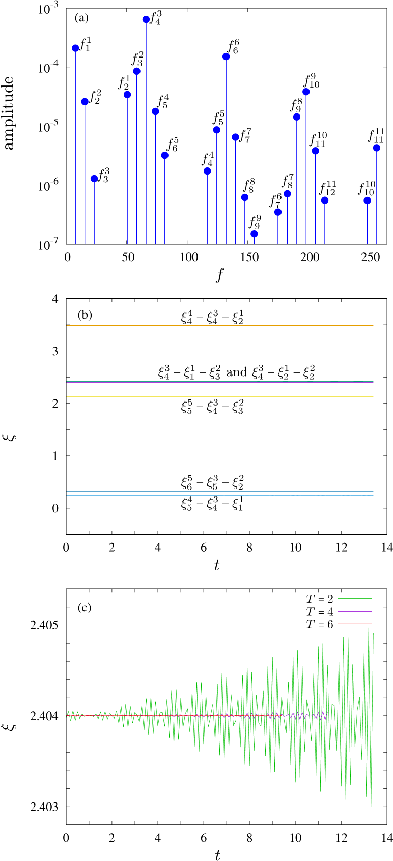
Figure 3: Analysis for a 2T MRW with $m=1$ azimuthal symmetry at ${\rm Ha}=3.5$. (a) Leading frequencies and amplitudes of the time series of poloidal component of the different modes $(m,l)$. The frequency $f^{m}_{l}$ corresponds to the main peak of the frequency spectrum of the time series of $\Re{\Phi^{m}_{l}(r_{d})}$. (b) Phase coupling among the different modes corresponding to different types of resonances shown in Table 1. The phase of each frequency $f^{m}_{l}$ is $\xi^{m}_{l}$. (c) The coupling $\xi^{3}_{4}=\xi^{1}_{1}+\xi^{2}_{3}$ is investigated by a time-dependent frequency analysis with time windows of length $T$.

Figure 3(a) shows the frequencies $f^{m}_{l}$ involved in Table 1 versus their corresponding amplitudes. The relations $f^{m_{0}}_{m_{0}}<f^{m_{0}+1}_{m_{0}+1}$ and $f^{m_{0}}_{m_{0}+1}<f^{m_{0}+1}_{m_{0}+2}$ are verified for all $m_{0}=1,..,11$ meaning that low wave numbers have smaller frequencies (slow modes) and larger wave numbers have larger frequencies (fast modes). The figure shows however that no clear threshold between slow and fast modes can be defined. In contrast to the results in Barik et al. (2018), where only resonances between one slow and two fast modes are reported, we find resonances between slow modes (e. g. $f^{3}_{3}=f^{1}_{1}+f^{2}_{2}$), fast and slow modes (e. g. $f^{11}_{11}=f^{1}_{1}+f^{10}_{10}$), and fast modes (e. g. $f^{10}_{10}=f^{4}_{4}+f^{6}_{6}$).

Figures 3(b) and (c) correspond to the analysis of the phase coupling among the resonant modes, described in § IV.1. Concretely, the time dependent relations given in Eq. (9) are displayed in Fig. 3(b) for some resonant triads. The time window used for this figure is $T=2$ over a time series covering the interval $[0,15]$. The phase coupling is satisfied up to an accuracy which is similar to that for the frequency determination as it is demonstrated in Fig. 3(c). The latter figure shows that the tiny variation of $\xi^{3}_{4}-\xi^{1}_{1}-\xi^{2}_{3}$ decreases as the size of the time window $T$ increases, i. e. as the accuracy of the frequency determination increases.

IV.3 Path to triadic resonances from unstable rotating waves

Unstable RWs with azimuthal symmetry $m=4$ bifurcate from the axisymmetric base state at a Hartmann number ${\rm Ha}=11.04<{\rm Ha}_{c}=12.2$ (see Garcia and Stefani (2018)), where ${\rm Ha}_{c}$ is the critical value predicted by the linear theory (Travnikov, Eckert, and Odenbach (2011)). These RWs again correspond to the radial jet instability. Because the linear eigenfunctions are equatorially antisymmetric, and RWs are nonlinear solutions, these RWs are equatorially asymmetric. They have however a particular structure (as happened for RWs described in § IV.2) since the $m=4k$ modes are equatorially antisymmetric (resp. symmetric) when $k$ is an odd (resp. even) integer number. Then, if $\omega$ is the rotation frequency of the RW the spherical harmonic amplitudes for the poloidal field of Eq. (5) read

$$\Phi_{l}^{4k}(r,t)=\overline{\Phi}_{l}^{4k}(r)~{}e^{-i4k\omega t},$$ (11)

with $\overline{\Phi}_{l}^{4k}(r)=0$ when $k+l$ is an odd integer number.

A secondary Hopf bifurcation (see Garcia et al. (2020b) gives rise to 2T MRWs with the same azimuthal symmetry and the same mode structure. In this case the spherical harmonic amplitudes $\Phi_{l}^{4k}(r,t)$ become quasiperiodic of the form

$$\Phi_{l}^{4k}(r,t)=\overline{\Phi}_{l}^{4k}(t,r)~{}e^{-i4k\omega t},$$ (12)

with $\overline{\Phi}_{l}^{4k}(t,r)$ being a periodic function with $\overline{\Phi}_{l}^{4k}(t,r)=0$ when $k+l$ is an odd integer number, and $\omega$ the rotation frequency of the MRW (e. g. Rand (1982)).

Because of these structures, both RWs and MRWs, fulfill the triadic resonance conditions for the azimuthal wave number $m$:

$$f^{4}_{5}=f^{12}_{13}-f^{8}_{8}=f^{16}_{16}-f^{12}_{13}=f^{20}_{21}-f^{16}_{16}=...,$$ (13)

where the frequencies $f^{m}_{l}$ correspond to those of largest amplitude in the frequency spectrum of the time series of $\Re{\Phi^{m}_{l}(r_{d})}$. As in the previous section, for each azimuthal mode $m=4k$, $k=1,2,...$, there is a latitudinal mode $l$ which verify the resonance condition. For instance the relation $f^{4}_{5}=f^{16}_{16}-f^{12}_{13}$ given above corresponds to $f^{4}_{5}=f^{16}_{18}-f^{12}_{13}$, since $f^{16}_{18}=f^{16}_{16}$.

By further varying the Hartmann number a tertiary Hopf bifurcation gives rise to 3T MRWs, i. e. quasiperiodic flows with three incommensurable frequencies. By means of this bifurcation the $m=4$ azimuthal symmetry is broken and the new MRWs acquire azimuthal symmetry $m=2$. In contrast to MRWs with $m=4$ azimuthal symmetry, all the azimuthal modes $m$ are now equatorially asymmetric, meaning that $\Phi^{m}_{m}(t,r),\Phi^{m}_{m+1}(t,r),....,\Phi^{m}_{L_{\text{max}}}(t,r)$ are nonzero. The dominant azimuthal wave numbers for this solution are $m=4,2,8,6,10,12$ (see Fig. (5) of Garcia et al. (2020b)) so we focus on studying the resonances among these modes. We have identified several relations between the frequencies $f^{m}_{l}$, which are listed in Table 2. These relations include those of Eq. (13) found for the parent RWs and MRWs. The fact that bifurcated solutions conserve the resonance relations was also found in the scenario studied in § IV.2. As will be evidenced in the following this is indeed true for further bifurcations found in Garcia et al. (2020b).

Table 2: Relations between the main frequencies $f^{m}_{l}$ of the different modes $(m,l)$ for the 3T MRW with $m=2$ azimuthal symmetry at ${\rm Ha}=1.6$.

$m=4$	$m=6$	$m=8$	$m=10$	$m=12$
$f^{4}_{4}=2f^{2}_{3}$	$f^{6}_{6}=f^{2}_{2}+f^{4}_{4}=f^{2}_{3}+f^{4}_{5}$	$f^{8}_{8}=f^{2}_{2}+f^{6}_{6}=f^{2}_{3}+f^{6}_{7}=2f^{4}_{5}$	$f^{10}_{10}=f^{2}_{2}+f^{8}_{8}=f^{4}_{5}+f^{6}_{7}$	$f^{12}_{12}=f^{2}_{2}+f^{10}_{10}=2f^{6}_{7}$
$f^{4}_{5}=f^{2}_{2}+f^{2}_{3}$	$f^{6}_{7}=f^{2}_{2}+f^{4}_{5}$	$f^{8}_{9}=f^{2}_{3}+f^{6}_{6}=f^{4}_{4}+f^{4}_{5}$	$f^{10}_{11}=f^{2}_{2}+f^{8}_{9}=f^{2}_{3}+f^{8}_{8}$	$f^{12}_{13}=f^{2}_{2}+f^{10}_{11}=f^{2}_{3}+f^{10}_{10}$
			$\hskip 14.22636pt=f^{4}_{4}+f^{6}_{7}=f^{4}_{5}+f^{6}_{6}$	$\hskip 14.22636pt=f^{4}_{5}+f^{8}_{8}=f^{6}_{6}+f^{6}_{7}$

After a quaternary Hopf bifurcation, totally breaking the azimuthal symmetry, quasiperiodic MRWs with four incommensurable frequencies develop and the resonance relations for the same 4T MRW analyzed in Garcia et al. (2020b), at ${\rm Ha}=1.4$, are provided in Table 3. There are less relations when comparing with Table 1 of § IV.2, obtained for a 2T MRW, which seems reasonable since the time dependence is now more complex as illustrated in figure 4(a,b). The time series of $\Re{\Phi^{m}_{l}(r_{d})}$ have now several comparable peaks in their frequency spectrum so the selection of the frequency $f^{m}_{l}$ becomes less clear (compare Fig. 1(c) with Fig. 4(c)).

Table 3: Relations between the main frequencies $f^{m}_{l}$ of the different modes $(m,l)$ for the 4T MRW with $m=1$ azimuthal symmetry at ${\rm Ha}=1.4$ and a chaotic flow with $m=1$ azimuthal symmetry at ${\rm Ha}=0.5$. For $m=3$ only the relation $f^{3}_{3}=f^{1}_{1}+f^{2}_{2}$ has been found. Note that these relations contain those for the 3T MRW with $m=2$ azimuthal symmetry shown in Table 2. These relations are satisfied up to $(f^{m_{0}}_{l_{0}}-f^{m_{1}}_{l_{1}}-f^{m_{2}}_{l_{2}})/f^{m_{0}}_{l_{0}}<\epsilon_{f}$ with $\epsilon_{f}=4\times 10^{-5}$ for the 4T MRW and with $\epsilon_{f}=1.5\times 10^{-4}$ for the chaotic flow.

$m=4$	$m=5$	$m=6$	$m=7$	$m=8$	$m=9$	$m=10$	$m=11$	$m=12$
$f^{4}_{4}=2f^{2}_{3}$	$f^{5}_{5}=f^{2}_{3}+f^{3}_{4}$	$f^{6}_{6}=f^{1}_{1}+f^{5}_{5}$	$f^{7}_{7}=f^{2}_{2}+f^{5}_{5}$	$f^{8}_{8}=f^{1}_{1}+f^{7}_{7}$	$f^{9}_{9}=f^{2}_{2}+f^{7}_{7}$	$f^{10}_{10}=f^{1}_{1}+f^{9}_{9}$	$f^{11}_{11}=f^{1}_{1}+f^{10}_{10}$	$f^{12}_{12}=f^{2}_{2}+f^{10}_{10}$
		$\hskip 11.38109pt=f^{2}_{2}+f^{4}_{4}$	$\hskip 11.38109pt=f^{2}_{3}+f^{5}_{6}$	$\hskip 11.38109pt=f^{2}_{2}+f^{6}_{6}$	$\hskip 11.38109pt=f^{3}_{4}+f^{6}_{7}$	$\hskip 14.22636pt=f^{2}_{2}+f^{8}_{8}$	$\hskip 14.22636pt=f^{3}_{3}+f^{8}_{8}$	$\hskip 14.22636pt=f^{3}_{3}+f^{9}_{9}$
		$\hskip 11.38109pt=f^{2}_{3}+f^{4}_{5}$	$\hskip 11.38109pt=f^{3}_{4}+f^{4}_{5}$	$\hskip 11.38109pt=f^{2}_{3}+f^{6}_{7}$	$\hskip 11.38109pt=f^{4}_{5}+f^{5}_{6}$	$\hskip 14.22636pt=f^{3}_{3}+f^{7}_{7}$	$\hskip 14.22636pt=f^{4}_{5}+f^{7}_{8}$	$\hskip 14.22636pt=f^{5}_{6}+f^{7}_{8}$
				$\hskip 11.38109pt=f^{3}_{3}+f^{5}_{5}$		$\hskip 14.22636pt=f^{3}_{4}+f^{7}_{8}$		$\hskip 14.22636pt=2f^{6}_{7}$
				$\hskip 11.38109pt=2f^{4}_{5}$		$\hskip 14.22636pt=f^{4}_{5}+f^{6}_{7}$
$f^{4}_{5}=f^{1}_{1}+f^{3}_{4}$	$f^{5}_{6}=f^{2}_{2}+f^{3}_{4}$	$f^{6}_{7}=f^{1}_{1}+f^{5}_{6}$	$f^{7}_{8}=f^{1}_{1}+f^{6}_{7}$	$f^{8}_{9}=f^{2}_{3}+f^{6}_{6}$	$f^{9}_{10}=f^{2}_{3}+f^{7}_{7}$	$f^{10}_{11}=f^{1}_{1}+f^{9}_{10}$	$f^{11}_{12}=f^{2}_{2}+f^{9}_{10}$	$f^{12}_{13}=f^{1}_{1}+f^{11}_{12}$
$\hskip 11.38109pt=f^{2}_{2}+f^{2}_{3}$		$\hskip 11.38109pt=f^{2}_{2}+f^{4}_{5}$	$\hskip 11.38109pt=f^{3}_{3}+f^{4}_{5}$	$\hskip 11.38109pt=f^{4}_{4}+f^{4}_{5}$	$\hskip 14.22636pt=f^{3}_{4}+f^{6}_{6}$	$\hskip 14.22636pt=f^{2}_{2}+f^{8}_{9}$	$\hskip 14.22636pt=f^{2}_{3}+f^{9}_{9}$	$\hskip 14.22636pt=f^{2}_{2}+f^{10}_{11}$
		$\hskip 11.38109pt=f^{3}_{3}+f^{3}_{4}$			$\hskip 14.22636pt=f^{4}_{5}+f^{5}_{5}$	$\hskip 14.22636pt=f^{2}_{3}+f^{8}_{8}$	$\hskip 14.22636pt=f^{3}_{4}+f^{8}_{8}$	$\hskip 14.22636pt=f^{2}_{3}+f^{10}_{10}$
					$\hskip 14.22636pt=f^{4}_{4}+f^{5}_{6}$	$\hskip 14.22636pt=f^{4}_{4}+f^{6}_{7}$	$\hskip 14.22636pt=f^{4}_{5}+f^{7}_{7}$	$\hskip 14.22636pt=f^{3}_{3}+f^{9}_{10}$
						$\hskip 14.22636pt=f^{4}_{5}+f^{6}_{6}$	$\hskip 14.22636pt=f^{5}_{5}+f^{6}_{7}$	$\hskip 14.22636pt=f^{4}_{5}+f^{8}_{8}$
							$\hskip 14.22636pt=f^{5}_{6}+f^{6}_{6}$	$\hskip 14.22636pt=f^{5}_{5}+f^{7}_{8}$
								$\hskip 14.22636pt=f^{6}_{6}+f^{6}_{7}$

Figure 4: (a) The time series of $\Re{\Phi^{4}_{4}(r_{d})}$ is strongly modulated. (b) The time series for $\Re{\Phi^{4}_{5}(r_{d})}$ is slightly modulated. (c) The first ten frequencies of largest amplitude from the frequency spectrum of $\Re{\Phi^{4}_{4}(r_{d})}$ (squares) and of $\Re{\Phi^{4}_{5}(r_{d})}$ (circles). The peaks selected for the resonance relations shown in table 3 are labelled on the plot. The solution is a 4T MRW with $m=1$ azimuthal symmetry at ${\rm Ha}=1.4$.

The resonance relations found for the 3T MRWs prevail for the bifurcated 4T MRWs (all relations of Table 2 are included in Table 3). Moreover, the resonance relations for the 4T MRWs of Table 3 even prevail for chaotic flows bifurcated from these 4T MRWs. We have checked this by considering a chaotic flow at ${\rm Ha}=0.5$. As noticed in Garcia et al. (2020a, b) the main frequencies associated to the flow and to the volume-averaged properties remain nearly constant for a wide interval of Hartmann numbers, at which several types of 2T, 3T and 4T MRW can be found. Figure 5 evidences that this is also true for the frequencies $f^{m}_{l}$. Figure 5 shows from top to bottom the selected frequencies $f^{m}_{l}$ and amplitudes for the sequence of bifurcated solutions: 2T MRW and 3T MRW both at ${\rm Ha}=1.6$ (panel (a)), 4T MRW at ${\rm Ha}=1.4$ (panel (b)), and a chaotic flow at ${\rm Ha}=0.5$ (panel (c)). From this figure it is clear that $f^{m}_{l}$ are almost unchanged.

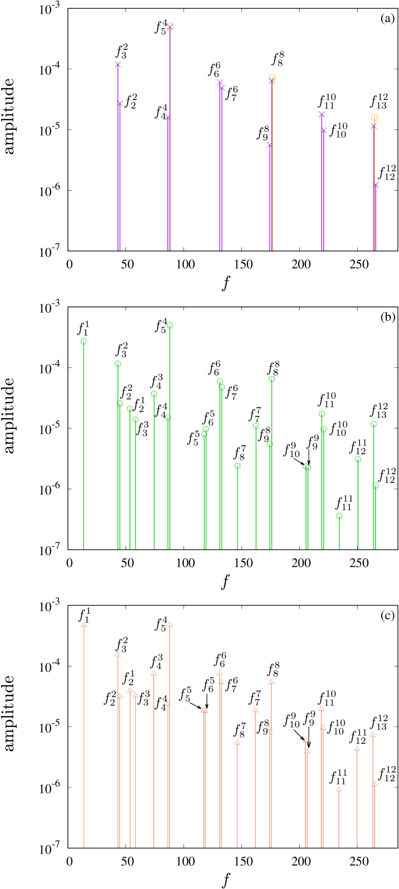
Figure 5: Leading frequencies and amplitudes of the time series of poloidal component of the different modes $(m,l)$. The frequency $f^{m}_{l}$ corresponds to one peak of the frequency spectrum of the time series of $\Re{\Phi^{m}_{l}(r_{d})}$, where $r_{d}=(r_{i}+r_{o})/2$. (a) The solutions are a 2T MRW with $m=4$ azimuthal symmetry (squares) and a 3T MRW with $m=2$ azimuthal symmetry (crosses), both at ${\rm Ha}=1.6$. (b) The solution is a 4T MRW with $m=1$ azimuthal symmetry (circles) at ${\rm Ha}=1.4$. (c) The solution is a chaotic wave with $m=1$ azimuthal symmetry (triangles) at ${\rm Ha}=0.5$.

Figure 6 is concerned with the analysis of the phase coupling among the resonant modes (see § IV.1) for the 4T MRW (top row) at ${\rm Ha}=1.4$ and for the chaotic flow at ${\rm Ha}=0.5$ (bottom row). In this bifurcation scenario the time dependence of the phase coupling relations $\xi^{m_{0}}_{l_{0}}-\xi^{m_{1}}_{l_{1}}-\xi^{m_{2}}_{l_{2}}$, although noticeable, is being damped as the time window $T$ increases. This means that for sufficiently large time windows the phase coupling tends to be verified. For the 4T and chaotic flow, the necessity of considering very large time windows ($T>10$) in time dependent frequency analysis has been already pointed out in Garcia et al. (2020b).

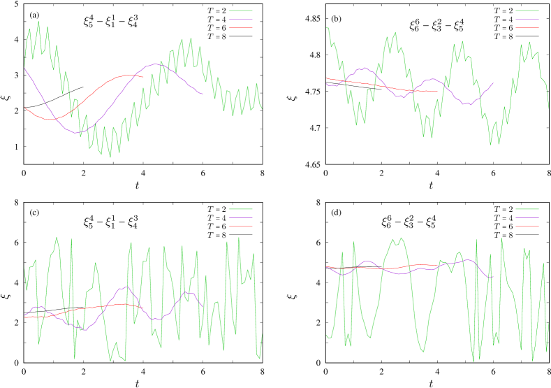
Figure 6: Phase coupling among the different modes corresponding to two different types of resonances $f^{4}_{5}=f^{1}_{1}+f^{3}_{4}$ and $f^{6}_{6}=f^{2}_{3}+f^{4}_{5}$ shown in Table 3. The phase of each frequency $f^{m}_{l}$ is $\xi^{m}_{l}$. The coupling is investigated by a time-dependent frequency analysis with time windows of length $T$. (a,c) The relation $\xi^{4}_{5}(t)-\xi^{1}_{1}(t)-\xi^{3}_{4}(t)$ tends to be roughly constant as the length of the time window $T$ increases. (b,d) The relation $\xi^{6}_{6}(t)-\xi^{2}_{3}(t)-\xi^{4}_{5}(t)$ is nearly constant as the length of the time window $T$ increases. (a,b) Correspond to a 4T MRW at ${\rm Ha}=1.4$ and (c,d) correspond to a chaotic wave at ${\rm Ha}=0.5$.

IV.4 Comparison with triadic resonances of inertial modes

We now compare quantitatively our results with the previous studies of Barik et al. (2018) and Lin (2021) in rotating spherical geometry for which triadic resonances, involving inertial modes, are described. In the first place we compare with the experiments and simulations of Barik et al. (2018) as the analyzed problem, the SC flow with a rotating inner (with $\Omega_{i}$) and outer (with $\Omega_{o}$) spheres, is a mechanically driven system equivalent to the problem considered here, the MSC flow. In the second place, we compare with the thermal convection problem in a full sphere of Lin (2021). Although we are contrasting problems with different types of driving or dynamical regimes the comparison makes sense since all the systems are SO$(2)\times$Z₂-equivariant.

The frequencies shown in Table 1 and fig. 3(a) are dimensionless. With the time scale $d^{2}/\nu$ considered in our modelling, dimensional frequencies, $f_{d}$, are obtained by $f_{d}=f\nu/d^{2}$ so

$$\frac{\omega_{d}}{\Omega_{i}}=\frac{2\pi f_{d}}{\Omega_{i}}=\frac{\omega}{{\rm Re}(\chi-1)},$$

with $\omega=2\pi f$. The ratios $\omega_{d}/\Omega_{i}$ are the angular frequences normalized by the angular frequency of rotation of the inner sphere since the outer sphere is at rest, $\Omega_{o}=0$. For the modes analyzed in fig. 3(a) the slowest mode is $(m,l)=(1,1)$ with a ratio $\omega_{d}/\Omega_{i}=0.097$. This value is very similar to that of the basic $m=1$ instability studied in Barik et al. (2018) with a ratio $\omega_{d}/\Omega_{o}=0.086$. In our case the fastest mode corresponds to $(m,l)=(11,11)$ with a ratio $\omega_{d}/\Omega_{i}=3.22$. The mode $(m,l)=(3,4)$, which has the largest peak in the frequency spectrum, has a ratio close to unity $\omega_{d}/\Omega_{i}=0.83$. In the case of the SC flow (Barik et al. (2018)) values in the range $(0.4,1)$ have been obtained for the ratio $\omega_{d}/\Omega_{o}$ in the case of fast inertial modes.

The development of triadic resonances for rotating thermal convection in a full sphere studied by Lin (2021) follows the same picture as investigated here. Rotating waves in the form of inertial modes with $m=4$ (e. g. Zhang (1993); Net, Garcia, and Sánchez (2008); Sánchez, Garcia, and Net (2016)) are the first time-dependent instabilities in the considered parameter regime (low Prandtl and Ekman numbers). Lin (2021) slightly increases the forcing parameter (the Rayleigh number) to obtain an azimuthally asymmetric quasiperiodic flow with two frequencies (see their Fig. 1), i. e. a 2T MRW with azimuthal symmetry $m=1$, for which resonant azimuthal modes have been found. The appearance of MRWs in rotating thermal convection in spherical shells due to a Hopf bifurcation from RWs is a generic scenario which has been studied in Garcia et al. (2015); Garcia, Net, and Sánchez (2016). In addition, and in agreement with our results, Lin (2021) has also found resonant behaviour for chaotic flows close to the onset.

For the inertial convective resonant solutions the value $\omega_{d}/\Omega$ has been also computed (see Table 1 of Lin (2021)) to identify fast and slow modes. By varying the Ekman and Prandtl numbers it was found that $|\omega_{d}/\Omega|\in(0.0899,0.5352$, either for the primary or free modes, which are $m=\{4,1,3\}$, $m=\{1,7,8\}$, and $m=\{3,10,13\}$ for the three different cases studied in Table 1 of Lin (2021). These results are indeed similar to the results for the radial jet instability (Secs. IV.2 and IV.3) since resonances involving these azimuthal wave numbers are found with values $\omega_{d}/\Omega_{i}$ of similar magnitude.

V Nonlinear interactions among latitudinal modes

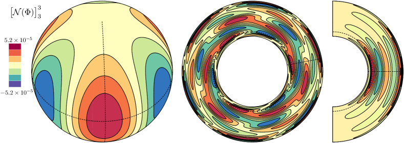
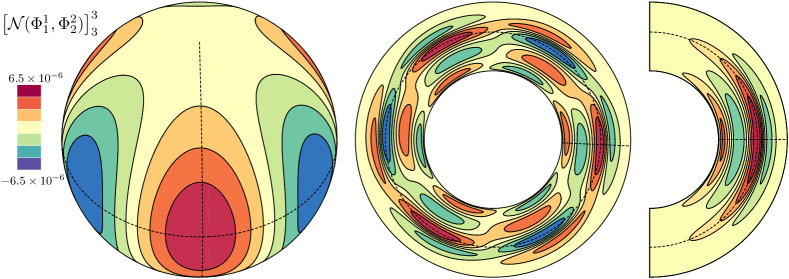
Figure 7: Contour plots on spherical, latitudinal and meridional sections through a local maximum for the $(m,l)=(3,3)$ component of the nonlinear term corresponding to the Navier-Stokes equations for the poloidal field. The evaluation of this nonlinear term is applied to the poloidal field whereas the toroidal field is set to zero. All the spherical harmonics amplitudes are considered for the poloidal field in the top row but only the modes $(m,l)=(1,1),(2,2)$ are considered in the bottom row. The solution is a 2T MRW with $m=1$ azimuthal symmetry at ${\rm Ha}=3.5$.

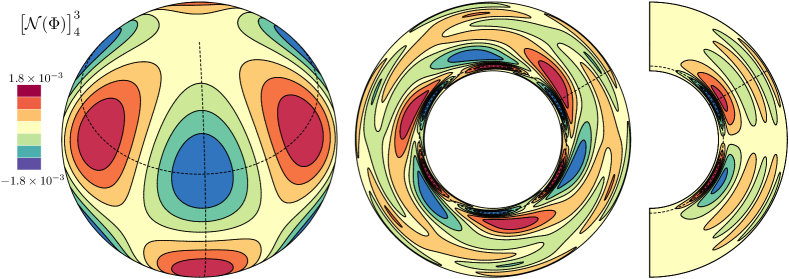
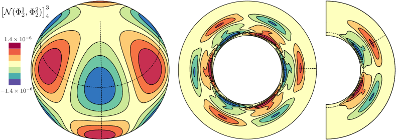
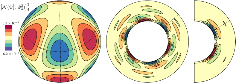
Figure 8: As figure 7 but for the $(m,l)=(3,4)$ component of the nonlinear term. In this figure the modes $(m,l)=(1,2),(2,2)$ and $(m,l)=(1,1),(2,3)$ are considered in the middle and bottom row. The solution is a 2T MRW with $m=1$ azimuthal symmetry at ${\rm Ha}=3.5$.

The quadratic nonlinear nature of the advection term in the Navier-Stokes equations provides a way to to understand the development of the different resonances obtained in § IV.2 and § IV.3. The azimuthal coupling among the different resonant waves has been already described in § III and we now focus on the latitudinal coordinate.

The product of the spherical harmonics expansion (e. g. Eq. (5)) gives rise to products of associated Legendre functions $P^{m_{1}}_{l_{1}}(\cos{\theta})P^{m_{2}}_{l_{2}}(\cos{\theta})\equiv P^{m_{1}}_{l_{1}}P^{m_{2}}_{l_{2}}$ which can be expressed in terms of a linear combination of associated Legendre functions of order $m_{1}+m_{2}$ and appropriate degree $l$ (see Hwang (1995)):

$$P^{m_{1}}_{l_{1}}P^{m_{2}}_{l_{2}}=\sum_{l=0}^{\big{[}\nu/2\big{]}}D_{l_{1}+l_{2}-2l}P^{m_{1}+m_{2}}_{l_{1}+l_{2}-2l},$$ (14)

where $\nu=l_{1}+l_{2}-m_{1}-m_{2}$ and $\big{[}\cdot\big{]}$ means the integer part. In this way, for certain $l$ we may seek for all the products $P^{m_{1}}_{l_{1}}P^{m_{2}}_{l_{2}}$ for which $P^{m_{1}+m_{2}}_{l_{1}+l_{2}-2l}$ appears in the linear combination of Eq. (14). We are thus searching for modes $(m_{i},l_{i})$, $i=1,2$, which “feed” -by means of the products $P^{m_{1}}_{l_{1}}P^{m_{2}}_{l_{2}}$- the mode $(m,l)=(m_{1}+m_{2},l_{1}+l_{2}-2l)$. Some of the found modes $(m_{i},l_{i})$ are in resonance with the “feeded” mode $(m,l)=(m_{1}+m_{2},l_{1}+l_{2}-2l)$.

The linear combinations of Eq.(14) are tabulated in the appendix of Hwang (1995), up to degree $5$, and help us to exemplify the relation between resonances and nonlinear interaction of the modes. For example, by looking for the products which feed $(m,l)=(3,3)$ we find

$$P^{2}_{2}P^{1}_{1}=g(P^{3}_{3}),~{}P^{2}_{3}P^{1}_{2}=g(P^{3}_{5},P^{3}_{3}),$$ (15)

where $g$ is a linear function different for each product. One of these relations provide the resonance condition $f^{3}_{3}=f^{1}_{1}+f^{2}_{2}$. We note that we have excluded products such as

$$P^{1}_{3}P^{2}_{2}=g(P^{3}_{5},P^{3}_{3}),~{}P^{1}_{4}P^{2}_{3}=g(P^{3}_{7},P^{3}_{5},P^{3}_{3}),$$

since they are equivalent to those of Eq.(15) in the sense that for the modes $(1,1)$ and $(1,3)$ (resp. $(1,2)$ and $(1,4)$) the same frequency can be selected $f^{1}_{1}=f^{1}_{3}$ (resp. $f^{1}_{2}=f^{1}_{4}$), as they both represent the equatorially symmetric (resp. equatorially antisymmetric) part of the $m=1$ mode. We have also not considered the coupling with the $m=0$ mode.

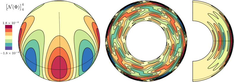
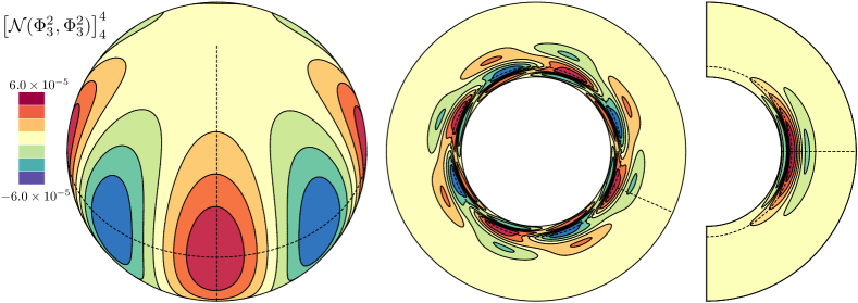
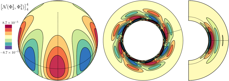
Figure 9: As figure 7 but for the $(m,l)=(4,4)$ component of the nonlinear term. In this figure the modes $(m,l)=(2,3),(2,3)$ and $(m,l)=(1,2),(3,4)$ are considered in the middle and bottom row. The solution is a 2T MRW with $m=1$ azimuthal symmetry at ${\rm Ha}=3.5$.

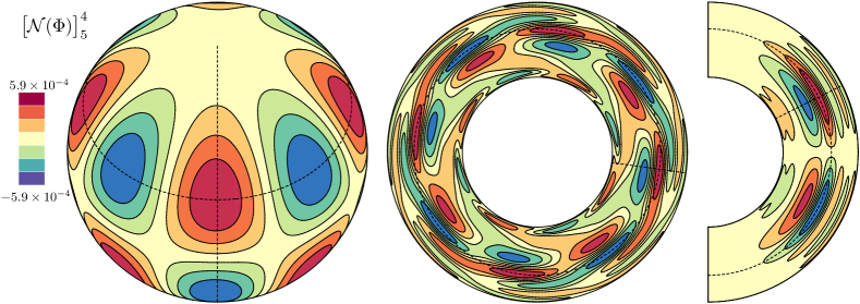
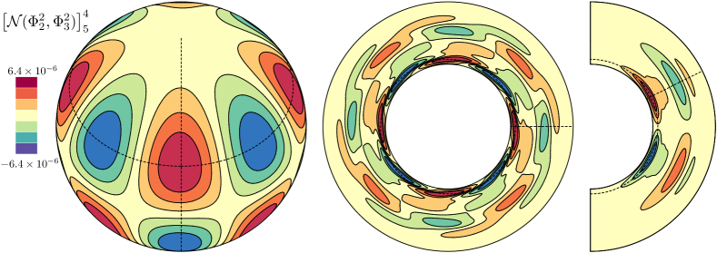
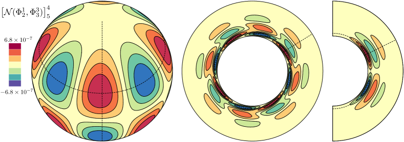
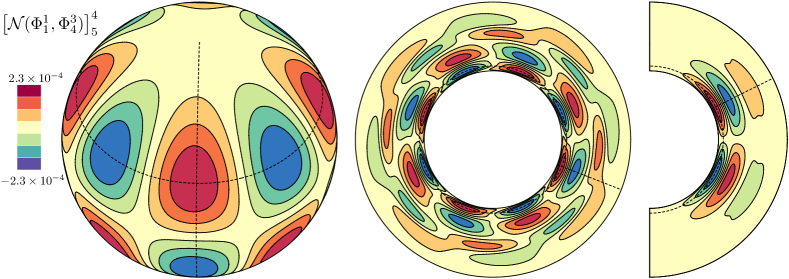
Figure 10: As figure 7 but for the $(m,l)=(4,5)$ component of the nonlinear term. In this figure the modes $(m,l)=(2,2),(2,3)$, the modes $(m,l)=(1,2),(3,3)$, and the modes $(m,l)=(1,1),(3,4)$, are considered in the 2nd, 3rd, and 4th rows, respectively. The solution is a 2T MRW with $m=1$ azimuthal symmetry at ${\rm Ha}=3.5$.

In case of the $(m,l)=(3,4)$ mode the situation is analogous and the products feeding this mode are

$$P^{2}_{2}P^{1}_{2}=g(P^{3}_{4}),~{}P^{2}_{3}P^{1}_{1}=g(P^{3}_{4}),~{}P^{2}_{3}P^{1}_{1}=g(P^{3}_{4}),$$

for which both resonance relations have been found (see Table 1) in the scenario studied in § IV.2. For the azimuthal wave number $m=4$ the products feeding the $(4,4)$ mode are

$$P^{2}_{2}P^{2}_{2}=g(P^{4}_{4}),~{}P^{2}_{3}P^{2}_{3}=g(P^{4}_{6},P^{4}_{4}),$$

$$P^{3}_{3}P^{1}_{1}=g(P^{4}_{4}),~{}P^{3}_{4}P^{1}_{2}=g(P^{4}_{6},P^{4}_{4})$$

and for the $(4,5)$ mode are

$$P^{2}_{3}P^{2}_{2}=g(P^{4}_{5}),~{}P^{3}_{3}P^{1}_{2}=g(P^{4}_{5}),~{}P^{3}_{4}P^{1}_{1}=f(P^{4}_{5}).$$

As in the case for the $m=3$ wave number the resonances found for the $(4,4)$ and $(4,5)$ modes arise from the above relationships. We have also checked the case $m=5$.

To further investigate the coupling between the resonant modes for the poloidal field we compute its associated nonlinear term from the Navier-Stokes equation, i. e.,

$$\mathcal{N}({\mathbf{v}})={\rm Re}~{}\mathbf{r}\cdot\nabla\times\nabla\times{\bf{\mathbf{w}}\times{\mathbf{v}}},$$ (16)

but with only considering the poloidal component when computing the velocity ${\mathbf{v}}$, and vorticity ${\mathbf{w}}$ fields (i. e. we set the toroidal field to zero $\Psi\equiv 0$), so $\mathcal{N}\equiv\mathcal{N}(\Phi)$. We then compare the spatial patterns of the scalar $\mathcal{N}(\Phi)$ obtained by using all the modes in the spherical harmonic expansion of the poloidal field (Eq. (5)), with the patterns of $\mathcal{N}(\Phi)$ obtained from a poloidal field with only nonzero amplitudes for a selected set of two resonant modes. As it is shown in the following, the set of two resonant modes provides a first order approximation of the patterns obtained with the full spherical harmonic expansion. For the pattern comparison we have considered the 2T MRW with $m=1$ azimuthal symmetry at ${\rm Ha}=3.5$, the resonances of which have been studied in § IV.2, concretely in table 1.

The first row of figure 7 displays the contour plots of $\big{[}\mathcal{N}(\Phi)\big{]}^{3}_{3}$, i. e., the spherical harmonic amplitude $(m,l)=(3,3)$ of the nonlinear term given in Eq. 16, on spherical, meridional and latitudinal sections (from left two right). The position of the sections, marked with dashed lines, matches the position of a local maxima. The second row shows the corresponding contour plots of $\big{[}\mathcal{N}(\Phi)\big{]}^{3}_{3}$ for the case that only the amplitudes $(m,l)=(1,1),(2,2)$ of the poloidal field are non-zero. The similarity between the radial structure among the two rows is a clear indication that the nonlinear interaction of the $(1,1)$ and $(2,2)$ resonant modes is sufficient to provide a first order approximation of the nonlinear term feeding the equatorially symmetric $(3,3)$ mode. Figure 8 summarises the comparison in the case of the modes which are resonant with the equatorially antisymmetric mode $(3,4)$ (shown in the first row). These are the modes $(1,2),(2,2)$ and $(1,1),(2,3)$ displayed in the middle and bottom row, respectively.

The patterns of the nonlinear terms in the case of the resonant modes with azimuthal wave number $m=4$ are displayed in Fig. 9, for the equatorially symmetric $(4,4)$ mode, and in Fig 10, for the equatorially antisymmetric $(4,5)$ mode, respectively. The patterns for the resonant modes $(2,3),(2,3)$ and $(1,2),(3,4)$ and those obtained from the full spherical harmonics expansion match only close to the inner boundary, so non-resonant modes should be considered to approximate the nonlinear term close to the outer boundaries. For the equatorially antisymmetric mode $(4,5)$ the resonant modes provide a reasonable approximation of the nonlinear term.

VI Conclusions

A comprehensive frequency analysis of several equatorially symmetric and antisymmetric poloidal modes has been presented for different types of weakly magnetic spherical Couette flows, in the context of the radial jet instability (Hollerbach, Junk, and Egbers (2006); Travnikov, Eckert, and Odenbach (2011); Garcia and Stefani (2018)). Two different bifurcation scenarios have been considered to evidence the mechanisms for the development of resonant triads among modes $(m,l)$, having different spherical harmonic order $m$ and degree $l$.

The first scenario comprises the first, second and third bifurcations from the base state giving rise to stable flows. The second scenario involves up to five bifurcations giving rise to either unstable or stable flows. In both scenarios the sequence of bifurcations includes the path:

$$\text{base state}\rightarrow\text{RWs}\rightarrow\text{2T-MRWs}\rightarrow\text{3T-MRWs}$$

for which the right arrows indicate Hopf bifurcations, which may break the azimuthal symmetry of the flow. The above sequence of bifurcations is generic in SO$(2)\times$Z₂-equivariant systems when the first bifurcation breaks the axisymmetry of the base state. In this case, RWs are the first time dependent solutions (e. g. Rand (1982); Crawford and Knobloch (1991); Golubitsky, LeBlanc, and Melbourne (2000)).

The type of time dependence of a RW, for which the main time scale is associated to a solid body rotation of a flow pattern, allows to define $\overline{\varphi}=\varphi+\omega t$, with $\omega$ being the rotation frequency of the wave, so the mathematical description in terms of spherical harmonics become equivalent to solutions of the inviscid equation (Greenspan (1968)). This is also true for MRW which are quasiperiodic flows with two incommensurate frequencies for which, due to the nonlinear coupling, resonance relations can be defined following similar arguments as those given in Barik et al. (2018).

For all the MRW explored, which have the azimuthal symmetry broken, a multitude of resonance relations, both in terms of spherical harmonic order $m$ and degree $l$, are found. We have considered modes of the type $(m,m)$ and $(m,m+1)$ to investigate the role of the equatorially symmetric and antisymmetric part of the flow. In addition, we have analyzed the nonlinear interactions giving rise to triadic resonances in terms of Legendre polynomials.

The phase coupling among resonant modes, pointed out in Hoff, Harlander, and Triana (2016) and further investigated in Barik et al. (2018), is a consequence of the regularity of MRW, as they are quasiperiodic solutions. For this type of solutions, frequency spectra do not depend on time (Garcia et al. (2021)). In addition, triadic resonances are observed for chaotic flows originated from further bifurcations of MRWs. This is because the main two frequencies of these chaotic flows are very similar to those of the MRW, from which they bifurcate (Garcia et al. (2020a, b)). Because of this, triadic resonances are very common for the radial jet instability of the MSC flow.

The results of the present study are compared with previous studies devoted to triadic resonances in spherical systems. In the case of spherical Couette flow resonant modes have been studied in Barik et al. (2018) and for rotating thermal convection in full spheres resonant solutions are investigated in Lin (2021). In contrast to these studies, for which all the free resonant modes are inertial and the base mode is strongly geostrophic, our simulations demonstrate the existence of resonances between modes which are neither geostrophic nor inertial, but related with the radial jet instability.

The existence of triadic resonances in spherical systems can thus be explained in terms of bifurcation theory since they are associated to the existence of MRW. In this framework, we argue that an inertial regime is not a requirement for the development of resonant triads as our results point out. We remark that in spherical systems the interpretation of resonances in terms of MRW, i. e. equivariant dynamical systems theory, is not in contradiction with the interpretation in terms of inertial waves since MRWs in the inertial regime have been found in the case of rotating thermal convection (e. g. Garcia, Chambers, and Watts (2019); Lin (2021)).

We finally note that MRW are common in rotating convective spherical shells (e. g. Garcia et al. (2015); Garcia, Net, and Sánchez (2016)) in a regime in which the onset of convection is of columnar type (Zhang (1992)). We have checked that for these type of MRW resonant triads also occur.

Data availability

The data that support the findings of this study are available from the corresponding author upon reasonable request.

References

- Albrecht et al. (2015) Albrecht, T., Blackburn, H. M., Lopez, J. M., Manasseh, R., and Meunier, P., “Triadic resonances in precessing rapidly rotating cylinder flows,” J. Fluid Mech. 778, R1 (2015).
- Albrecht et al. (2018) Albrecht, T., Blackburn, H. M., Lopez, J. M., Manasseh, R., and Meunier, P., “On triadic resonance as an instability mechanism in precessing cylinder flow,” J. Fluid Mech. 841, R3 (2018).
- Barik et al. (2018) Barik, A., Triana, S. A., Hoff, M., and Wicht, J., “Triadic resonances in the wide-gap spherical Couette system,” J. Fluid Mech. 843, 211–243 (2018).
-
Borland et al. (2017)
Borland, M., Emery, L., Shang, H., and Soliday, R., (2017), User’s Guide for SDDS Toolkit
Version 3.51, It is available on the web at
https://ops.aps.anl.gov/manuals/SDDStoolkit/SDDStoolkit.html. - Brunet, Gallet, and Cortet (2020) Brunet, M., Gallet, B., and Cortet, P.-P., “Shortcut to geostrophy in wave-driven rotating turbulence: The quartetic instability,” Phys. Rev. Lett. 124, 124501 (2020).
- Campagne et al. (2019) Campagne, A., Hassaini, R., Redor, I., Valran, T., Viboud, S., Sommeria, J., and Mordant, N., “Identifying four-wave-resonant interactions in a surface gravity wave turbulence experiment,” Phys. Rev. Fluids 4, 074801 (2019).
- Chandrasekhar (1981) Chandrasekhar, S., Hydrodynamic and Hydromagnetic Stability (Dover publications, inc. New York, 1981).
- Coughlin and Marcus (1992) Coughlin, K. T. and Marcus, P. S., “Modulated waves in Taylor-Couette flow. Part 1. Analysis,” J. Fluid Mech. 234, 1–18 (1992).
- Crawford and Knobloch (1991) Crawford, J. D. and Knobloch, E., “Symmetry and symmetry-breaking bifurcations in fluid dynamics,” Annu. Rev. Fluid Mech. 23, 341–387 (1991).
- Ecke, Zhong, and Knobloch (1992) Ecke, R. E., Zhong, F., and Knobloch, E., “Hopf bifurcation with broken reflection symmetry in rotating Rayleigh-Bénard convection,” Europhys. Lett. 19, 177–182 (1992).
- Frigo and Johnson (2005) Frigo, M. and Johnson, S. G., “The design and implementation of FFTW3,” Proceedings of the IEEE 93, 216–231 (2005), special issue on "Program Generation, Optimization, and Platform Adaptation".
- Galtier (2003) Galtier, S., “Weak inertial-wave turbulence theory,” Phys. Rev. E 68, 015301 (2003).
- Garcia, Chambers, and Watts (2019) Garcia, F., Chambers, F. R. N., and Watts, A. L., “Polar waves and chaotic flows in thin rotating spherical shells,” Phys. Rev. Fluids 4, 074802 (2019).
- Garcia et al. (2010) Garcia, F., Net, M., García-Archilla, B., and Sánchez, J., “A comparison of high-order time integrators for thermal convection in rotating spherical shells,” J. Comput. Phys. 229, 7997–8010 (2010).
- Garcia, Net, and Sánchez (2016) Garcia, F., Net, M., and Sánchez, J., “Continuation and stability of convective modulated rotating waves in spherical shells,” Phys. Rev. E 93, 013119 (2016).
- Garcia et al. (2015) Garcia, F., Sánchez, J., Dormy, E., and Net, M., “Oscillatory convection in rotating spherical shells: Low Prandtl number and non-slip boundary conditions.” SIAM J. Appl. Dynam. Systems 14, 1787–1807 (2015).
- Garcia et al. (2019) Garcia, F., Seilmayer, M., Giesecke, A., and Stefani, F., “Modulated rotating waves in the magnetized spherical Couette system,” J. Nonlinear Sci. 29, 2735–2759 (2019).
- Garcia et al. (2020a) Garcia, F., Seilmayer, M., Giesecke, A., and Stefani, F., “Chaotic wave dynamics in weakly magnetised spherical Couette flows,” Chaos 30, 043116 (2020a).
- Garcia et al. (2020b) Garcia, F., Seilmayer, M., Giesecke, A., and Stefani, F., “Four-frequency solution in a magnetohydrodynamic Couette flow as a consequence of azimuthal symmetry breaking,” Phys. Rev. Lett. 125, 264501 (2020b).
- Garcia et al. (2021) Garcia, F., Seilmayer, M., Giesecke, A., and Stefani, F., “Long term time dependent frequency analysis of chaotic waves in the weakly magnetised spherical Couette system,” Physica D Accepted (2021).
- Garcia and Stefani (2018) Garcia, F. and Stefani, F., “Continuation and stability of rotating waves in the magnetized spherical Couette system: Secondary transitions and multistability,” Proc. R. Soc. A 474, 20180281 (2018).
- Giesecke et al. (2015) Giesecke, A., Albrecht, T., Gundrum, T., Herault, J., and Stefani, F., “Triadic resonances in nonlinear simulations of a fluid flow in a precessing cylinder,” New J. Phys 17, 113044 (2015).
- Golubitsky, LeBlanc, and Melbourne (2000) Golubitsky, M., LeBlanc, V. G., and Melbourne, I., “Hopf bifurcation from rotating waves and patterns in physical space,” J. Nonlinear Sci. 10, 69–101 (2000).
- Golubitsky and Stewart (2003) Golubitsky, M. and Stewart, I., The Symmetry Perspective: From Equilibrium to Chaos in Phase Space and Physical Space. (Birkhäuser, Basel, 2003).
- Goto and van de Geijn (2008) Goto, K. and van de Geijn, R. A., “Anatomy of high-performance matrix multiplication,” ACM Trans. Math. Softw. 34, 1–25 (2008).
- Greenspan (1968) Greenspan, H. P., The theory of rotating fluids (Cambridge University Press, 1968).
- Hammack and Henderson (1993) Hammack, J. L. and Henderson, D. M., “Resonant interactions among surface water waves,” Annu. Rev. Fluid Mech. 25, 55–97 (1993).
- Herault et al. (2015) Herault, J., Gundrum, T., Giesecke, A., and Stefani, F., “Subcritical transition to turbulence of a precessing flow in a cylindrical vessel,” Phys. Fluids 27, 124102 (2015).
- Hoff, Harlander, and Triana (2016) Hoff, M., Harlander, U., and Triana, S. A., “Study of turbulence and interacting inertial modes in a differentially rotating spherical shell experiment,” Phys. Rev. Fluids 1, 043701 (2016).
- Hollerbach (2009) Hollerbach, R., “Non-axisymmetric instabilities in magnetic spherical Couette flow,” Proc. R. Soc. A 465, 2003–2013 (2009).
- Hollerbach et al. (2004) Hollerbach, R., Futterer, B., More, T., and Egbers, C., “Instabilities of the Stewartson layer. Part 2. Supercritical mode transitions,” Theoret. Comput. Fluid Dynamics 18, 197–204 (2004).
- Hollerbach, Junk, and Egbers (2006) Hollerbach, R., Junk, M., and Egbers, C., “Non-axisymmetric instabilities in basic state spherical Couette flow,” Fluid Dyn. Res. 38, 257–273 (2006).
- Hwang (1995) Hwang, C., “A method for computing the coefficients in the product-sum formula of associated Legendre functions,” J. Geod. 70, 110–116 (1995).
- Jones (2011) Jones, C. A., “Planetary magnetic fields and fluid dynamos,” Annu. Rev. Fluid Mech. 43, 583–614 (2011).
- Kelley et al. (2007) Kelley, D. H., Triana, S. A., Zimmerman, D. S., Tilgner, A., and Lathrop, D. P., “Inertial waves driven by differential rotation in a planetary geometry,” Geophys. Astrophys. Fluid Dynamics 101, 469–487 (2007).
- Kuznetsov (1998) Kuznetsov, Y. A., Elements of Applied Bifurcation Theory, Second Edition (Springer, New York, 1998).
- Lagrange, Nadal, and Eloy (2011) Lagrange, R. Meunier, P., Nadal, F., and Eloy, C., “Precessional instability of a fluid cylinder,” J. Fluid Mech. 666, 104–145 (2011).
- Laskar (1990) Laskar, J., “The chaotic motion of the solar system: A numerical estimate of the size of the chaotic zones,” Icarus 88, 266 – 291 (1990).
- Laskar (1993) Laskar, J., “Frequency analysis of a dynamical system,” Celestial Mech. Dyn. Astron. 56, 191–196 (1993).
- Laskar, Froeschlé, and Celletti (1992) Laskar, J., Froeschlé, C., and Celletti, A., “The measure of chaos by the numerical analysis of the fundamental frequencies. application to the standard mapping,” Physica D 56, 253 – 269 (1992).
- Le Bars, Cébron, and Le Gal (2015) Le Bars, M., Cébron, D., and Le Gal, P., “Flows driven by libration, precession, and tides,” Annu. Rev. Fluid Mech. 47, 163–193 (2015).
- Li et al. (2020) Li, J., Liu, Z., Liao, S., and Borthwick, A. G. L., “Steady-state multiple near resonances of periodic interfacial waves with rigid boundary,” Phys. Fluids 32, 087104 (2020).
- Lin (2021) Lin, Y., “Triadic resonances driven by thermal convection in a rotating sphere,” J. Fluid Mech. 909, R3 (2021).
- Lopez and Marques (2018) Lopez, J. M. and Marques, F., “Rapidly rotating precessing cylinder flows: forced triadic resonances,” J. Fluid Mech. 839, 239–270 (2018).
- Net, Garcia, and Sánchez (2008) Net, M., Garcia, F., and Sánchez, J., “On the onset of low-Prandtl-number convection in rotating spherical shells: non-slip boundary conditions,” J. Fluid Mech. 601, 317–337 (2008).
- Ogbonna et al. (2020) Ogbonna, J., Garcia, F., Gundrum, T., Seilmayer, M., and Stefani, F., “Experimental investigation of the return flow instability in magnetized spherical Couette flows,” Phys. Fluids 32, 124119 (2020).
- Plevachuk et al. (2014) Plevachuk, Y., Sklyarchuk, V., Eckert, S., Gerbeth, G., and Novakovic, R., “Thermophysical properties of the liquid Ga-In-Sn eutectic alloy,” J. Chem. Eng. Data 59, 757–763 (2014).
- Rand (1982) Rand, D., “Dynamics and symmetry. Predictions for modulated waves in rotating fluids,” Arch. Ration. Mech. Anal. 79, 1–37 (1982).
- Rieutord and Valdettaro (1997) Rieutord, M. and Valdettaro, L., “Inertial waves in a rotating spherical shell,” J. Fluid Mech. 341, 77–99 (1997).
- Sánchez, Garcia, and Net (2013) Sánchez, J., Garcia, F., and Net, M., “Computation of azimuthal waves and their stability in thermal convection in rotating spherical shells with application to the study of a double-Hopf bifurcation,” Phys. Rev. E 87, 033014/ 1–11 (2013).
- Sánchez, Garcia, and Net (2016) Sánchez, J., Garcia, F., and Net, M., “Critical torsional modes of convection in rotating fluid spheres at high taylor numbers,” J. Fluid Mech. 791 (2016), 10.1017/jfm.2016.52.
- Sánchez and Net (2016) Sánchez, J. and Net, M., “Numerical continuation methods for large-scale dissipative dynamical systems,” Eur. Phys. J. Spec. Top. 225, 2465–2486 (2016).
- Sisan et al. (2004) Sisan, D. R., Mujica, N., Tillotson, W. A., Huang, Y. M., Dorland, W., Hassam, A. B., Antonsen, T. M., and Lathrop, D. P., “Experimental observation and characterization of the magnetorotational instability,” Phys. Rev. Lett. 93, 114502 (2004).
- Smith and Waleffe (1999) Smith, L. M. and Waleffe, F., “Transfer of energy to two-dimensional large scales in forced, rotating three-dimensional turbulence,” Phys. Fluids 11, 1608–1622 (1999).
- Stewartson (1966) Stewartson, K., “On almost rigid rotations. Part 2.” J. Fluid Mech. 26, 131–144 (1966).
- Sutherland and Jefferson (2020) Sutherland, B. R. and Jefferson, R., “Triad resonant instability of horizontally periodic internal modes,” Phys. Rev. Fluids 5, 034801 (2020).
- Travnikov, Eckert, and Odenbach (2011) Travnikov, V., Eckert, K., and Odenbach, S., “Influence of an axial magnetic field on the stability of spherical Couette flows with different gap widths,” Acta Mech. 219, 255–268 (2011).
- Waleffe (1992) Waleffe, F., “The nature of triad interactions in homogeneous turbulence,” Physics of Fluids A: Fluid Dynamics 4, 350–363 (1992).
- Wicht (2014) Wicht, J., “Flow instabilities in the wide-gap spherical Couette system,” J. Fluid Mech. 738, 184–221 (2014).
- Zhang (1992) Zhang, K., “Spiralling columnar convection in rapidly rotating spherical fluid shells,” J. Fluid Mech. 236, 535–556 (1992).
- Zhang (1993) Zhang, K., “On equatorially trapped boundary inertial waves,” J. Fluid Mech. 248, 203–217 (1993).
- Zhang et al. (2001) Zhang, K., Earnshaw, P., Liao, X., and F.H., B., “On inertial waves in a rotating fluid sphere,” JFM 437, 103–119 (2001).
- Zhang and Liao (2017) Zhang, K. and Liao, X., Theory and Modeling of Rotating Fluids: Convection, Inertial Waves and Precession, Cambridge Monographs on Mechanics (Cambridge University Press, 2017).