The Page Curve for Fermionic Gaussian States

Abstract

In a seminal paper, Page found the exact formula for the average entanglement entropy for a pure random state. We consider the analogous problem for the ensemble of pure fermionic Gaussian states, which plays a crucial role in the context of random free Hamiltonians. Using recent results from random matrix theory, we show that the average entanglement entropy of pure random fermionic Gaussian states in a subsystem of $N_{A}$ out of $N$ degrees of freedom is given by $\langle S_{A}\rangle_{\mathrm{G}}\!=\!(N\!-\!\tfrac{1}{2})\Psi(2N)\!+\!(\tfrac{1}{4}\!-\!N_{A})\Psi(N)\!+\!(\tfrac{1}{2}\!+\!N_{A}\!-\!N)\Psi(2N\!-\!2N_{A})\!-\!\tfrac{1}{4}\Psi(N\!-\!N_{A})\!-\!N_{A}$, where $\Psi$ is the digamma function. Its asymptotic behavior in the thermodynamic limit is given by $\langle S_{A}\rangle_{\mathrm{G}}\!=\!N(\log 2-1)f+N(f-1)\log(1-f)+\tfrac{1}{2}f+\tfrac{1}{4}\log{(1-f)}\,+\,O(1/N)$, where $f=N_{A}/N$. Remarkably, its leading order agrees with the average over eigenstates of random quadratic Hamiltonians with number conservation, as found by Łydżba, Rigol and Vidmar. Finally, we compute the variance in the thermodynamic limit, given by the constant $\lim_{N\to\infty}(\Delta S_{A})^{2}_{\mathrm{G}}=\frac{1}{2}(f+f^{2}+\log(1-f))$.

Introduction.—Entanglement is a hallmark of quantum theory bell1964einstein ; bell1966problem . The study of the von Neumann bipartite entanglement entropy plays a central role in the quantum foundations of statistical mechanics deutsch_91 ; srednicki_94 ; rigol_dunjko_08 ; d2016quantum ; gogolin2016equilibration ; deutsch2018eigenstate ; goldstein_lebowitz_06 ; popescu_short_06 ; tasaki_98 ; polkovnikov2011colloquium ; vidmar2017entanglement ; liu2018quantum ; vidmar2018volume ; hackl2019average ; Vidmar:2017pak ; bianchi2019typical ; lydzba2020eigenstate ; lydzba2021entanglement ; bernard2021entanglement , in quantum information theory Hayden:2006 ; Hayden:2007cs ; Sekino:2008he ; Hosur:2015ylk ; Roberts:2016hpo ; Fujita:2017pju ; Lu:2017tbo ; Fujita:2018wtr , in the formulation of the black hole information puzzle Page:1993wv ; Giddings:2012bm ; Braunstein:2009my ; Almheiri:2012rt ; Marolf:2017jkr ; Harlow:2014yka ; Bianchi:2014bma ; Abdolrahimi:2015tha , and the study of the quantum nature of spacetime geometry VanRaamsdonk:2010pw ; Bianchi:2012ev ; Jacobson:2015hqa ; Bianchi_2019 ; Baytas:2018wjd ; Qi:2018ogs . Also experimentally there has been recently tremendous progress in measuring entanglement entropy in optical lattices with ultracold atoms greiner_mandel_02b .

In a seminal paper page1993average , Page showed that, when an isolated quantum system is in a random pure state, the average entanglement entropy of a subsystem is close to maximal. In particular, he conjectured an exact formula for the average, taken with respect to the Haar measure over states in a finite-dimensional Hilbert space. In this letter we address the analogous problem for the ensemble of pure fermionic Gaussian states. We compute the average entanglement entropy $\braket{S_{A}}_{\mathrm{G}}$ of those states (6) and study its properties (figure 1) with the help of random matrix theory.

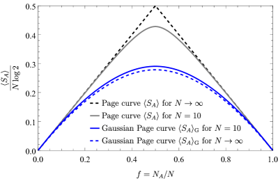
Figure 1: We compare the Page curve for random states $\braket{S_{A}}$ to the Page curve for random Gaussian states $\braket{S_{A}}_{\mathrm{G}}$ for a system with $N$ fermionic degrees of freedom.

Pure fermionic Gaussian states appear as ground states and eigenstates of free, i.e., quadratic, Hamiltonians, and remain Gaussian in the time evolution after a free quantum quench fagotti2008evolution ; alba2018entanglement . They play an important role in quantum computing in the context of matchgates valiant2002quantum . Moreover, there has been an increased interest in fermionic Gaussian states from the perspective of quantum chaos srednicki_94 , and the eigenstate thermalization hypothesis rigol_dunjko_08 ; vidmar16 ; magan2016random . The average eigenstate entanglement is of particular interest in this context vidmar2017entanglement ; vidmar2018volume ; hackl2019average , where one averages the entanglement entropy over the discrete set of eigenstates, which are Gaussian states for a given quadratic Hamiltonian. Our main results, the average entropy (6) and particularly its thermodynamic limit (7), unveil close relations to recent work on the average entanglement entropy of eigenstates of quadratic Hamiltonians liu2018quantum ; lydzba2020eigenstate ; lydzba2021entanglement . In particular, our formula (7) coincides in the thermodynamic limit with the average of the entanglement entropy with respect to the eigenstates of random quadratic Hamiltonians with number conservation (later numerically confirmed in lydzba2021entanglement to also apply to random Hamiltonians without number conservation).

The Page curve.— Before we come to the fermionic Gaussian states, let us briefly recall Page’s result. In a quantum system consisting of $N$ spin $1/2$ fermions, a subsystem of $N_{A}$ fermions (with $N=N_{A}+N_{B}$ and $N_{A}\leq N_{B}$) defines a bipartition of the Hilbert space of states as $\mathcal{H}=\mathcal{H}_{A}\otimes\mathcal{H}_{B}$, with dimensions $\dim\mathcal{H}_{A}=2^{N_{A}}$ and $\dim\mathcal{H}_{B}=2^{N_{B}}$. Given a pure state $\ket{\psi}\in\mathcal{H}$, the entanglement entropy of the subsystem is $S_{A}(\ket{\psi})=-\operatorname{Tr}(\rho_{A}\log\rho_{A})$ with $\rho_{A}=\operatorname{Tr}_{B}\ket{\psi}\!\bra{\psi}$ the induced density operator where the other $N_{B}$ fermions are traced out. The average over all states in $\mathcal{H}$ is

$$\braket{S_{A}}=\int\!d\mu(\psi)\,S_{A}(\ket{\psi})=\int_{U\in U(2^{N})}dU\;S_{A}(U\!\ket{0})\,,$$ (1)

where $d\mu(\psi)$ is the uniform measure in $\mathcal{H}$. This uniform measure on the $2^{2N}-1$ dimensional sphere can be obtained by fixing an arbitrary reference state $\ket{0}$ and acting on it with a unitary transformation $U$ distributed uniformly with respect to the Haar measure $dU$ over the unitary group $U\in U(2^{N})$. In page1993average , Page conjectured the formula (later proven in foong1994proof ; sanchez1995simple ; Sen:1996ph )

$$\textstyle\braket{S_{A}}=\Psi(2^{N}+1)-\Psi(2^{N-N_{A}}+1)-\frac{2^{N_{A}}-1}{2^{N-N_{A}+1}}\,,$$ (2)

where $\Psi(z)=\Gamma^{\prime}(z)/\Gamma(z)$ is the digamma function.

In the thermodynamic limit $N\to\infty$ with finite subsystem fraction $f=N_{A}/N\leq 1/2$, the average entropy reduces to

$$\textstyle\braket{S_{A}}\sim fN\log 2\,-\,\frac{1}{2}\,\mathrm{e}^{\,-(1-2f)N\log 2}\,.$$ (3)

Thence, for $f<1/2$, the average entanglement entropy approaches exponentially the entropy of a maximally mixed state. Similarly, in the thermodynamic limit, the dispersion around the average vivo_pato_16 ; wei2017proof ; bianchi2019typical scales as

$$\textstyle\Delta S_{A}\sim\begin{cases}\;2^{-(1-f)N-\frac{1}{2}}&0<f<\frac{1}{2}\\[5.0pt] \;2^{-\frac{1}{2}N-1}&f=\frac{1}{2}\end{cases}$$ (4)

and vanishes exponentially. Consequently, a typical state in the Hilbert space is extremely close to being maximally entangled.

Let us turn our focus to fermionic Gaussian states which are states annihilated by a set of fermionic annihilation operators. Given a reference Gaussian state $\ket{J_{0}}$, all Gaussian states $\ket{J_{M}}$ can be generated via Bogoliubov transformations. These states form a submanifold in the manifold of pure states. The uniform measure $d\mu_{\mathrm{G}}(J)$ over Gaussian states can be defined in terms of the Haar measure over Bogoliubov transformation, i.e., real orthogonal transformations $M\in O(2N)$ hackl2020bosonic . The average entanglement entropy over fermionic Gaussian states is then

$$\braket{S_{A}}_{\mathrm{G}}=\int\!\!d\mu_{\mathrm{G}}(J)\,S_{A}(\ket{J})=\!\int_{M\in O(2N)}dM\;S_{A}(\ket{J_{M}})\,.$$ (5)

Using random matrix theory, we derive the following exact formula for the average entanglement entropy:

$$\begin{split}\textstyle\braket{S_{A}}_{\mathrm{G}}&=(N\!-\!\tfrac{1}{2})\Psi(2N)+(\tfrac{1}{2}\!+\!N_{A}\!-\!N)\Psi(2N\!-\!2N_{A})\\[5.0pt] &\quad+(\tfrac{1}{4}\!-\!N_{A})\Psi(N)-\tfrac{1}{4}\Psi(N\!-\!N_{A})-N_{A}\,.\end{split}$$ (6)

In the thermodynamic limit $N\to\infty$ with finite fraction $f=N_{A}/N\leq 1/2$, a series expansion in $N$ yields

$$\begin{split}\braket{S_{A}}_{\mathrm{G}}&\sim N\,\big{(}(\log{2}\!-\!1)f+\!(f\!-\!1)\log(1\!-\!f)\big{)}\\[5.0pt] &\quad+\tfrac{1}{2}f+\tfrac{1}{4}\log{(1-f)}\,+\,O(1/N)\,,\end{split}$$ (7)

whose leading order term agrees with the expression deduced in lydzba2020eigenstate for the average over a different set of states, as we will review in our discussion. We also find that the standard deviation approaches the constant

$$\lim_{N\to\infty}(\Delta S_{A})_{\mathrm{G}}=\sqrt{\frac{f+f^{2}+\log(1-f)}{2}}\,.$$ (8)

We outline the derivation of these results in the ensuing discussion.

Average entropy.—A quantum system with $N$ fermionic degrees of freedom can be formulated in terms of a set of creation and annihilation operators $\hat{a}_{i}^{\dagger}$ and $\hat{a}_{i}$ with canonical anti-commutation relations, $\{\hat{a}_{i},\hat{a}_{j}^{\dagger}\}=\delta_{ij}$, $\{\hat{a}_{i},\hat{a}_{j}\}=0$ and $i,j=1\ldots N$. Equivalently, we can introduce $2N$ Majorana modes $\hat{\xi}_{\mu}$ with $\mu=1\ldots 2N$ and

$$\textstyle\hat{\xi}_{i}=\frac{1}{\sqrt{2}}(\hat{a}^{\dagger}_{i}+\hat{a}_{i})\quad\text{and}\quad\hat{\xi}_{N+i}=\frac{\operatorname{i}}{\sqrt{2}}(\hat{a}^{\dagger}_{i}-\hat{a}_{i})\,.$$ (9)

A Bogoliubov transformation $\hat{a}^{\prime}_{i}=\sum^{N}_{j=1}(\alpha_{ij}\hat{a}_{j}+\beta_{ij}\hat{a}_{j}^{\dagger})$ transforms the operators $\hat{\xi}_{\mu}$ to the new ones $\hat{\xi}_{\mu}^{\prime}$ according to $\hat{\xi}_{\mu}^{\prime}=\sum^{2N}_{\nu=1}M_{\mu\nu}\,\hat{\xi}_{\nu}$, where the $2N\times 2N$ matrix $M_{\mu\nu}$ is given by windt2020local

$$M=\begin{pmatrix}\operatorname{Re}(\alpha+\beta)&\operatorname{Im}(\beta-\alpha)\\ \operatorname{Im}(\alpha+\beta)&\operatorname{Re}(\alpha-\beta)\end{pmatrix}\,.$$ (10)

The requirement that the anti-commutation relations are preserved is equivalent to the condition $MM^{\intercal}=\mathbb{1}$, i.e., $M$ must be an orthogonal matrix in $O(2N)$.

To define the uniform average over fermionic Gaussian states, we exploit the notion of a complex structure $J$ (i.e., $J^{2}=-1$) and its relation to the correlation function hackl2020bosonic . The starting point is that a fermionic Gaussian state is defined as the ground state of a set of annihilation operators. We call $\ket{J_{0}}$ the state annihilated by the reference operators $\hat{a}_{i}$ and $\ket{J}$ the state annihilated by the Bogoliubov-transformed operators $\hat{a}^{\prime}_{i}$, i.e., $\hat{a}^{\prime}_{i}|J\rangle=0$. The label $J$ stands for the matrix $J=MJ_{0}M^{-1}$ determined by the expectation value of the commutator of two Majorana modes hackl2020bosonic ,

$$\braket{J}{\,[\hat{\xi}_{\mu},\hat{\xi}_{\nu}]\,}{J}=\operatorname{i}\,J_{\mu\nu}\quad\text{with}\quad J_{0}=\left(\begin{array}[]{c|c}0&\mathbb{1}\\ \hline\cr-\mathbb{1}&0\end{array}\right)\,.$$ (13)

The entanglement entropy of a Gaussian state $\ket{J}$ is directly related to the spectrum of the $2N_{A}\times 2N_{A}$ left-upper sub-block $[J]_{A}$ of $J$ via the formula $S_{A}(\ket{J})=\sum^{N_{A}}_{i=1}s(x_{i})$ with Peschel2003 ; Peschel2009 ; hackl2020bosonic ; windt2020local

$$s(x)=-\left(\tfrac{1-x}{2}\right)\log\left(\tfrac{1-x}{2}\right)-\left(\tfrac{1+x}{2}\right)\log\left(\tfrac{1+x}{2}\right)\,,$$ (14)

where $x_{i}\in[0,1]$ are the singular values of $[J]_{A}$.

Having defined fermionic Gaussian states in terms of a reference state $\ket{J_{0}}$ and an orthogonal matrix $M$, we can express the uniform measure over Gaussian states in terms of the Haar measure over $O(2N)$ and compute the average entanglement entropy of Gaussian states exploiting (5). What we need to derive first is the joint probability distribution of the singular values $x_{i}$ of $[J]_{A}$. For this purpose we make repetitive use of (kieburg2019multiplicative, , Proposition A.2) by projecting away always two rows of the matrix $J$; first to $[J]_{N-1}$, then $[J]_{N-2}$ until we arrive at $[J]_{N_{A}}$. This yields for $x=(x_{1},\dots,x_{N_{A}})$ the distribution

$$\textstyle P(x)=\frac{\left(\det X\right)^{2}}{N_{A}!}\Big{(}\prod^{N_{A}-1}_{j=0}c_{j}^{-1}(1-x_{j+1}^{2})^{\Delta}\Big{)}\,,$$ (15)

where we have the $N_{A}\times N_{A}$ matrix $X$ and $c_{j}$,

$$X_{ij} =p_{j-1}(x_{i})=\mathcal{P}^{(\Delta,\Delta)}_{2j-2}(x_{i})\,,$$ (16)

$$c_{j} =\frac{2^{2\Delta}\,[(2j+\Delta)!]^{2}}{(2j)!\,(2j+2\Delta)!\,(4j+2\Delta+1)}\,,$$ (17)

$$\Delta =N_{B}-N_{A}\geq 0\,.$$ (18)

The functions $\mathcal{P}^{(\alpha,\beta)}_{n}(z)$ are the Jacobi polynomials and the distribution (15) is related to the Jacobi ensemble Forrester_2010 , one of the classical random matrix ensembles that can arise in various ways.

The $k$-point correlation functions Forrester_2010 encode the whole spectral statistics of a random matrix,

$$\textstyle R_{k}(x_{1},\dots,x_{k}) =\int P(x_{1},\dots,x_{k},y_{1},\dots,y_{N_{A}-k})d^{N_{A}-k}y$$

$$=\frac{(N_{A}-k)!}{N_{A}!}\det K(x_{a},x_{b})\,,$$ (19)

where $K(x_{a},x_{b})$ refers to the $k\times k$ matrix (with $a,b=1,\dots,k$) given by Forrester_2010

$$\begin{split}K(x,y)=\!\!\sum^{N_{A}-1}_{j=0}\!\psi_{j}(x)\psi_{j}(y),\,\,\,\psi_{j}(x)=\tfrac{(1-x^{2})^{\Delta/2}}{\sqrt{c_{j}}}p_{j}(x)\end{split}$$ (20)

with $\int_{0}^{1}\psi_{j}(x)\psi_{k}(x)dx=\delta_{jk}$. Then, the level density is $\rho(x)=R_{1}(x)=\frac{1}{N_{A}}K(x,x)=\frac{1}{N_{A}}\sum^{N_{A}-1}_{j=0}\psi^{2}_{j}(x)$.

The average entropy is then given by the integral

$$\braket{S_{A}}_{\mathrm{G}}=N_{A}\int_{0}^{1}s(x)\rho(x)$$ (21)

which can be evaluated by computing

$$I_{\epsilon}=\int^{1}_{-1}\left(\tfrac{x(1-x)^{\epsilon}}{2}-\tfrac{(1-x^{2})^{\epsilon}}{4}\right)\rho(|x|)\,dx\,,$$ (22)

such that $\braket{S_{A}}_{\mathrm{G}}=N_{A}\,(\partial_{\epsilon}I_{\epsilon}+\log{2})_{\epsilon\to 0}$. We combine the Jacobi polynomials with the other terms in the integrand whose integrals altogether give ratios of Gamma functions which, after the derivative yield the digamma functions in (6).

We can compare the Gaussian Page curve (6) with the original Page curve (2), as illustrated in figure 1. In the Gaussian case the thermodynamic limit is approached from above, while the original Page curve is approached from below. In fact, we can compute $\braket{S_{A}}=1/3$ and $\braket{S_{A}}_{\mathrm{G}}=1/2$ for $N_{A}=1$ with $N=2$, which shows that for small $N$ the average entanglement entropy of Gaussian states is above the one of all states. This is in stark contrast to the thermodynamic limit, where the average entanglement entropy of Gaussian states is almost half of the one for all states.

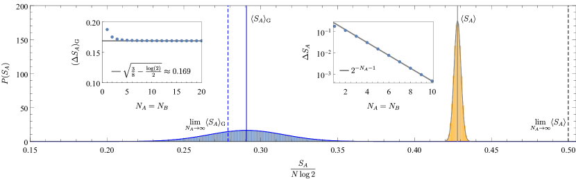
Figure 2: We compare the probability distributions $P(S_{A})$ of the entanglement entropy $S_{A}$ for Gaussian states and general states in a fermionic system with $N_{A}=N_{B}=5$. The expectation value $\braket{S_{A}}$ and $\braket{S_{A}}_{\mathrm{G}}$ for $N_{A}=N_{B}$ and their thermodynamic limits are indicated by vertical lines and vertical dashed lines, respectively. The insets depict the scaling of the standard deviation $\Delta S_{A}$ and $(\Delta S_{A})_{\mathrm{G}}$ for $N_{A}=N_{B}\to\infty$.

Variance.—An important question in the context of computing the average entanglement entropy is if this average is also typical, i.e., if almost all states have an entanglement entropy close to the average as we take the thermodynamic limit. To answer this question, we compute the variance $(\Delta S_{A})^{2}_{\mathrm{G}}=\braket{S_{A}^{2}}_{\mathrm{G}}-\braket{S_{A}}^{2}_{\mathrm{G}}$ of the probability distribution. For this, it is useful to define

$$\begin{split}s_{ij}&=\int^{1}_{0}s(x)\psi_{i}(x)\psi_{j}(x)dx\\ &=-\left(\partial_{\epsilon}\int^{1}_{-1}\left(\frac{1-x}{2}\right)^{1+\epsilon}\psi_{i}(x)\psi_{j}(x)dx\right)_{\epsilon\to 0}\,,\end{split}$$ (23)

where we used $\psi_{i}(x)=\psi_{i}(-x)$ to produce the two terms in (14) by integrating over $[-1,1]$. We can interpret $s_{ij}$ as the matrix elements of the operator $s(x)$ with respect to the orthonormal basis $\psi_{j}(x)$ in $[0,1]$. With this, we find

$$(\Delta S_{A})^{2}_{\mathrm{G}} =\int_{0}^{1}s^{2}(x)K(x,x)dx-\int_{0}^{1}s(x_{1})s(x_{2})K^{2}(x_{1},x_{2})d^{2}x=\int_{0}^{1}s(x_{1})s(x_{2})K(x_{1},x_{2})(\delta(x_{1}-x_{2})-K(x_{1},x_{2}))d^{2}x$$

$$=\int_{0}^{1}s(x)s(y)\left(\sum^{N_{A}-1}_{i=0}\psi_{i}(x_{1})\psi_{i}(x_{2})\right)\left(\sum^{\infty}_{j=N_{A}}\psi_{j}(x_{1})\psi_{j}(x_{2})\right)d^{2}x=\sum^{N_{A}-1}_{i=0}\sum^{\infty}_{j=N_{A}}s^{2}_{ij}\quad\text{with}$$ (24)

$$s^{2}_{ij} =\tfrac{(2j)!(2\Delta+4i+1)(\Delta+j+1)(2\Delta+2j+1)(2\Delta+4j+1)(2(\Delta+i))!\left((1+\Delta-2\Delta^{2})i-2(\Delta-1)i^{2}+(\Delta+1)(2j+1)(\Delta+j)\right)^{2}}{2(2i)!(2i-2j+1)^{2}(i-j)^{2}(-2i+2j+1)^{2}(2(\Delta+j+1))!(\Delta+i+j)^{2}(\Delta+i+j+1)^{2}(2\Delta+2i+2j+1)^{2}}\,\,\,\text{for}\,\,\,i<j\,,$$ (25)

where (25) is only valid for $i<j$, which is all we need for the sum in (27). Despite all terms in the sum of (27) are non-zero for large $N$, it is dominated by the summand $s^{2}_{N_{A}-1,N_{A}}$ (see figure 3, where we compare the sum vs. this dominating summand), so that it makes sense to consider the limit

$$\begin{split}\overline{s}^{2}_{lk}&=\lim_{N\to\infty}s^{2}_{N_{A}-1-l,N_{A}+k}\\ &=\tfrac{(\frac{1}{f}-1)^{-2(k+l+1)}(2k+2l+3-4f(k+l+1))^{2}}{4(k+l+1)^{2}(2k+2l+1)^{2}(2k+2l+3)^{2}}\end{split}$$ (26)

with fixed $f=N_{A}/N$. From this, we find the variance

$$\lim_{N\to\infty}(\Delta S_{A})^{2}_{\mathrm{G}}=\sum^{\infty}_{l,k=0}\overline{s}^{2}_{lk}=\frac{f+f^{2}+\log(1-f)}{2}\,,$$ (27)

where we could evaluate the sum analytically. That the variance approaches a constant is in line with numerical findings in lydzba2020eigenstate ; lydzba2021entanglement and analytical studies of Renyi entropies bernard2021entanglement . Recall that the Page variance $\Delta S_{A}$ from (4) converges to zero (with a behavior that differs for $f=\frac{1}{2}$), while the Gaussian standard deviation $(\Delta S_{A})_{\mathrm{G}}$ approaches a constant and only its relative dispersion $(\Delta S_{A})_{\mathrm{G}}/\braket{S_{A}}_{\mathrm{G}}$ will behave as $1/N$. In contrast, the standard deviation for (Gaussian) eigenstates of translationally invariant quadratic Hamiltonians was found in vidmar2017entanglement to scale as $\sqrt{N}$ (relative dispersion scaling as $1/\sqrt{N}$), which thus differs from both the Gaussian behavior found here and Page’s result.

The stark contrast of the behavior of the standard deviation for all states vs. Gaussian states, i.e., exponential vs. constant, is closely connected to the dimension of the respective family of states (see figure 2). While the real dimension of the manifold of pure fermionic states scales as $2^{N}$, the manifold of pure fermionic Gaussian states consists of two disconnected components of dimension $N(N-1)$ each. This behavior can be understood via Dyson’s Brownian motion where the number of eigenvalues of the underlying random matrix (exponential in $N_{A}$ for pure fermionic states and quadratic in $N_{A}$) is crucial for the rate of convergence.

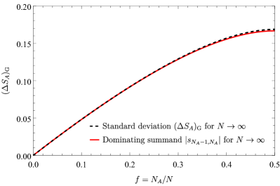
Figure 3: We compare the standard deviation $\lim_{N\to\infty}(\Delta S_{A})_{\mathrm{G}}$ from (27) with the leading summand $|\overline{s}_{0,0}|\!=\!\lim_{N\to\infty}|s_{N_{A}-1,N_{A}}|\!=\!\frac{(3-4f)f}{6(1-f)}$ from (26).

Relation to random Hamiltonians.—So far, we adopted the perspective of studying properties of a given ensemble of quantum states, namely the family of fermionic Gaussian states, without asking in what physical system one may necessarily encounter them. This is also the perspective of Page’s original paper page1993average where he considers the family of all pure states, without reference to a specific Hamiltonian. Remarkably, for Hamiltonians with local interactions, while the ground state is far from Page-typical as it generally satisfies an area law eisert2010colloquium , the entanglement entropy of energy eigenstates can be obtained from typicality arguments deutsch_91 ; srednicki_94 ; rigol_dunjko_08 ; d2016quantum ; gogolin2016equilibration ; deutsch2018eigenstate ; goldstein_lebowitz_06 ; popescu_short_06 ; tasaki_98 ; polkovnikov2011colloquium ; vidmar2017entanglement ; vidmar2018volume ; hackl2019average ; Vidmar:2017pak ; bianchi2019typical . Similarly, it is instructive to investigate for which random Hamiltonians the resulting ground states constitute the considered ensemble of fermionic Gaussian states discussed here.

For this aim, we consider the most general quadratic Hamiltonian for $N$ fermionic degrees of freedom,

$$\hat{H}=\!\!\!\sum_{i,j=1}^{N}\!(A_{ij}\hat{a}^{\dagger}_{i}\hat{a}_{j}\!+\!B_{ij}\hat{a}^{\dagger}_{i}\hat{a}_{j}^{\dagger}\!+{\rm h.c.})=\!\!\sum^{2N}_{\mu,\nu=1}\!\!\operatorname{i}h_{\mu\nu}\,\hat{\xi}_{\mu}\hat{\xi}_{\nu},$$ (28)

where the $2N$ Majorana modes were introduced in (9) and $h_{\mu\nu}$ is an anti-symmetric matrix with real entries (as also considered in lydzba2021entanglement ). Any such antisymmetric matrix can be block-diagonalized by means of an orthogonal transformation $M_{\mu\nu}$, such that

$$MhM^{-1}={\bigoplus}^{N}_{i=1}\begin{pmatrix}0&\omega_{i}\\ -\omega_{i}&0\end{pmatrix}\,,$$ (29)

where $\omega_{i}\geq 0$ leading to $\hat{H}=\sum^{N}_{i=1}\omega_{i}\,(\hat{b}_{i}^{\dagger}\hat{b}_{i}-\frac{1}{2})$ with transformed creation and annihilation operators.

If we randomly generate the matrix entries of $h_{\mu\nu}$ with respect to some $\mathrm{O}(2N)$ invariant probability distribution, for instance a Gaussian distribution, the orthogonal transformation $M$ that diagonalizes it will be Haar distributed. Therefore, the resulting ground state of $\hat{H}$ is the state annihilated by $\hat{b}_{i}$ and is distributed according to the ensemble of fermionic Gaussian states considered so far. Moreover, the excited energy eigenstates of this random Hamiltonian are also Gaussian states and distributed according to the same ensemble. Remarkably, the result does not depend on which specific choice of $\mathrm{O}(2N)$ invariant distribution we use to generate $\hat{H}$: in fact, only the one-particle spectrum $\omega_{i}$ depends on this choice, and the properties of the energy eigenstates are independent of the associated eigenvalues (as long as no degeneracies are present). Therefore, the eigenstates of (28) are distributed as random Gaussian states $\ket{J}$ with Haar measure $d\mu_{\mathrm{G}}(J)$ as in (5).

This result provides an analytical derivation of the numerical evidence found by Łydżba, Rigol and Vidmar in lydzba2021entanglement that in the thermodynamic limit the average entropy of eigenstates of a random Hamiltonian (28) is given by (7). Moreover, the argument above extents the result to systems of finite size: the average eigenstate entanglement entropy of $\mathrm{O}(2N)$-invariant random quadratic Hamiltonians is given by the exact analytic formula (6).

On the other hand, imposing further constraints on the Hamiltonian (28), such as requiring it to be particle number preserving or translationally invariant, will result in a submanifold of the manifold of fermionic Gaussian states (5). Therefore we cannot expect to find the same statistical properties (average, variance) for the entanglement entropy at finite system size. Yet, in the large $N$ limit, the average over eigenstates of number preserving Hamiltonians studied in  liu2018quantum ; lydzba2020eigenstate leads to an average entanglement entropy that agrees with our result (7) in the thermodynamic limit.

Discussion—The main result of this letter is the analytical expression (6), which is the analogue of Page’s result for the ensemble of fermionic Gaussian states for systems of finite size, and its large $N$ behavior (7). The derivation was made possible by recent advances in random matrix theory kieburg2019multiplicative , which bear promise to be also relevant for other ensembles of states. Our results enable us to deduce a number of interesting properties of the Page curve of fermionic Gaussian states: (a) The curve admits a closed form expression in terms of digamma functions from which finite size corrections to the thermodynamic limit can be extracted. (b) In contrast to Page’s typicality, for fermionic Gaussian states the thermodynamic limit is approached from above and only algebraically fast, rather than exponentially. (c) The variance approaches a constant at large $N$ rather than decaying exponentially as in Page’s case. (d) Finally, our result shows that whenever the subsystem fraction is finite in the thermodynamic limit, the average entanglement entropy is smaller than the maximal value $f\log 2$, but approaches it as the subsystem fraction $f$ goes to zero.

Our proof helps to clarify the relationship to the average entanglement entropy of ground states and eigenstates of random quadratic Hamiltonians, namely that these averages coincide in the thermodynamic limit provided that the Hamiltonian is sufficiently random. Let us emphasize that the function

$$\lim_{N\to\infty}\textstyle\frac{1}{N}\braket{S_{A}}_{\mathrm{G}}=(\log 2\!-\!1)f+(f\!-\!1)\log(1\!-\!f)$$ (30)

was found by Łydżba, Rigol and Vidmar in lydzba2020eigenstate as an average over energy eigenstates of random Hamiltonians with number conservation (and later shown numerically lydzba2021entanglement to also apply to eigenstates of random quadratic Hamiltonians without number conservation). In the thermodynamic limit, the associated level density of the matrix $[J]_{A}$ for a similar model was also found previously in liu2018quantum , from which the value $\lim_{N=2N_{A}\to\infty}\frac{1}{N}\braket{S_{A}}=\log{2}-\tfrac{1}{2}$ was computed. Both papers construct their family of states from number preserving quadratic Hamiltonians, namely either as the ground state of the SYK2 Hamiltonian liu2018quantum or as one of its eigenstates lydzba2020eigenstate . In both cases, the set of states is determined by the subgroup $\mathrm{U}(N)$ of number-preserving Bogoliubov transformations, which is only a submanifold of the $\mathrm{O}(2N)$ manifold of Gaussian states considered here. For $\mathrm{O}(2N)$-invariant random quadratic Hamiltonians, we find that the average eigenstate entanglement entropy is given by the analytic formula (6) for systems of finite size. Explaining from general arguments why in the thermodynamic limit the average (30) arises more generally, identifying what is the universality class and computing the finite size corrections to the average and variance for different classes of random Hamiltonians would be an interesting avenue for future work.

The random matrix techniques used here can also be applied to derive similar “Page-like curves” for Renyi entropies bernard2021entanglement and other information-theoretic quantities. While here we focused on energy eigenstates and time-independent Hamiltonians, our results provide also a prediction for the value of the equilibrium entanglement entropy under unitary evolution generated by a random time-dependent quadratic Hamiltonian fagotti2008evolution ; nahum2017quantum ; bauer2017stochastic .

Another Page-like curve was considered recently vidmar2017entanglement ; vidmar2018volume ; hackl2019average in the context of translationally invariant quadratic Hamiltonians, for which the average entanglement entropy over all eigenstates was computed. While this average involves a discrete set of states which differs depending on the chosen Hamiltonians, numerical evidence for several classes of translationally invariant quadratic models suggested the conjecture that the resulting curve is actually universal hackl2020bosonic in the thermodynamic limit. The most compelling explanation for such a behavior relies again on random matrix theory and assumes that any such discrete set will ultimately sample from the Haar measure on the manifold of translationally invariant Gaussian states. It would therefore be a meaningful avenue to adapt the methods developed in this letter to derive similar analytical expressions for the average entanglement entropy of translationally invariant Gaussian states.

- (1) J.S. Bell, On the Einstein Podolsky Rosen paradox, Physics Physique Fizika 1 (1964) 195.
- (2) J.S. Bell, On the problem of hidden variables in quantum mechanics, Reviews of Modern Physics 38 (1966) 447.
- (3) J.M. Deutsch, Quantum statistical mechanics in a closed system, Physical Review A 43 (1991) 2046.
- (4) M. Srednicki, Chaos and quantum thermalization, Physical Review E 50 (1994) 888 [cond-mat/9403051].
- (5) M. Rigol, V. Dunjko and M. Olshanii, Thermalization and its mechanism for generic isolated quantum systems, Nature 452 (2008) 854 [0708.1324].
- (6) L. D’Alessio, Y. Kafri, A. Polkovnikov and M. Rigol, From quantum chaos and eigenstate thermalization to statistical mechanics and thermodynamics, Advances in Physics 65 (2016) 239 [1509.06411].
- (7) C. Gogolin and J. Eisert, Equilibration, thermalisation, and the emergence of statistical mechanics in closed quantum systems, Reports on Progress in Physics 79 (2016) 056001 [1503.07538].
- (8) J.M. Deutsch, Eigenstate thermalization hypothesis, Reports on Progress in Physics 81 (2018) 082001 [1805.01616].
- (9) S. Goldstein, J.L. Lebowitz, R. Tumulka and N. Zanghì, Canonical typicality, Physical Review Letters 96 (2006) 050403 [cond-mat/0511091].
- (10) S. Popescu, A.J. Short and A. Winter, Entanglement and the foundations of statistical mechanics, Nature Physics 2 (2006) 754 [quant-ph/0511225].
- (11) H. Tasaki, From quantum dynamics to the canonical distribution: General picture and a rigorous example, Physical Review Letters 80 (1998) 1373 [1709.06259].
- (12) A. Polkovnikov, K. Sengupta, A. Silva and M. Vengalattore, Colloquium: Nonequilibrium dynamics of closed interacting quantum systems, Reviews of Modern Physics 83 (2011) 863 [1007.5331].
- (13) L. Vidmar, L. Hackl, E. Bianchi and M. Rigol, Entanglement entropy of eigenstates of quadratic fermionic hamiltonians, Physical Review Letters 119 (2017) 020601 [1703.02979].
- (14) C. Liu, X. Chen and L. Balents, Quantum entanglement of the Sachdev-Ye-Kitaev models, Physical Review B 97 (2018) 245126 [1709.06259].
- (15) L. Vidmar, L. Hackl, E. Bianchi and M. Rigol, Volume law and quantum criticality in the entanglement entropy of excited eigenstates of the quantum ising model, Physical Review Letters 121 (2018) 220602 [1808.08963].
- (16) L. Hackl, L. Vidmar, M. Rigol and E. Bianchi, Average eigenstate entanglement entropy of the xy chain in a transverse field and its universality for translationally invariant quadratic fermionic models, Physical Review B 99 (2019) 075123 [1812.08757].
- (17) L. Vidmar and M. Rigol, Entanglement entropy of eigenstates of quantum chaotic hamiltonians, Physical Review Letters 119 (2017) 220603 [1708.08453].
- (18) E. Bianchi and P. Donà, Typical entanglement entropy in the presence of a center: Page curve and its variance, Physical Review D 100 (2019) 105010 [1904.08370].
- (19) P. Łydżba, M. Rigol and L. Vidmar, Eigenstate entanglement entropy in random quadratic hamiltonians, Physical Review Letters 125 (2020) 180604 [2006.11302].
- (20) P. Łydżba, M. Rigol and L. Vidmar, Entanglement in many-body eigenstates of quantum-chaotic quadratic hamiltonians, Physical Review B 103 (2021) 104206 [2101.05309].
- (21) D. Bernard and L. Piroli, Entanglement distribution in the quantum symmetric simple exclusion process, arXiv preprint arXiv:2102.04745 (2021) [2102.04745].
- (22) P. Hayden, D.W. Leung and A. Winter, Aspects of generic entanglement, Communications in Mathematical Physics 265 (2006) 95 [quant-ph/0407049].
- (23) P. Hayden and J. Preskill, Black holes as mirrors: Quantum information in random subsystems, JHEP 09 (2007) 120 [0708.4025].
- (24) Y. Sekino and L. Susskind, Fast Scramblers, JHEP 10 (2008) 065 [0808.2096].
- (25) P. Hosur, X.-L. Qi, D.A. Roberts and B. Yoshida, Chaos in quantum channels, JHEP 02 (2016) 004 [1511.04021].
- (26) D.A. Roberts and B. Yoshida, Chaos and complexity by design, JHEP 04 (2017) 121 [1610.04903].
- (27) Y.O. Nakagawa, M. Watanabe, S. Sugiura and H. Fujita, Universality in volume-law entanglement of scrambled pure quantum states, Nature Communications 9 (2018) 1635 [1703.02993].
- (28) T.-C. Lu and T. Grover, Renyi Entropy of Chaotic Eigenstates, Physical Review E 99 (2019) 032111 [1709.08784].
- (29) H. Fujita, Y.O. Nakagawa, S. Sugiura and M. Watanabe, Page Curves for General Interacting Systems, JHEP 12 (2018) 112 [1805.11610].
- (30) D.N. Page, Information in black hole radiation, Physical Review Letters 71 (1993) 3743 [hep-th/9306083].
- (31) S.B. Giddings, Black holes, quantum information, and unitary evolution, Physical Review D 85 (2012) 124063 [1201.1037].
- (32) S.L. Braunstein, S. Pirandola and K. Życzkowski, Better Late than Never: Information Retrieval from Black Holes, Physical Review Letters 110 (2013) 101301 [0907.1190].
- (33) A. Almheiri, D. Marolf, J. Polchinski and J. Sully, Black Holes: Complementarity or Firewalls?, JHEP 02 (2013) 062 [1207.3123].
- (34) D. Marolf, The Black Hole information problem: past, present, and future, Reports on Progress in Physics 80 (2017) 092001 [1703.02143].
- (35) D. Harlow, Jerusalem Lectures on Black Holes and Quantum Information, Reviews of Modern Physics 88 (2016) 015002 [1409.1231].
- (36) E. Bianchi, T. De Lorenzo and M. Smerlak, Entanglement entropy production in gravitational collapse: covariant regularization and solvable models, JHEP 06 (2015) 180 [1409.0144].
- (37) S. Abdolrahimi and D.N. Page, Hawking Radiation Energy and Entropy from a Bianchi-Smerlak Semiclassical Black Hole, Physical Review D 92 (2015) 083005 [1506.01018].
- (38) M. Van Raamsdonk, Building up spacetime with quantum entanglement, General Relativity and Gravitation 42 (2010) 2323 [1005.3035].
- (39) E. Bianchi and R.C. Myers, On the Architecture of Spacetime Geometry, Classical and Quantum Gravity 31 (2014) 214002 [1212.5183].
- (40) T. Jacobson, Entanglement equilibrium and the einstein equation, Physical Review Letters 116 (2016) 201101 [1505.04753].
- (41) E. Bianchi, P. Donà and I. Vilensky, Entanglement entropy of bell-network states in loop quantum gravity: Analytical and numerical results, Physical Review D 99 (2019) 086013 [1812.10996].
- (42) B. Baytas, E. Bianchi and N. Yokomizo, Gluing polyhedra with entanglement in loop quantum gravity, Phys. Rev. D98 (2018) 026001 [1805.05856].
- (43) X.-L. Qi, Does gravity come from quantum information?, Nature Physics 14 (2018) 984.
- (44) M. Greiner, O. Mandel, T.W. Hänsch and I. Bloch, Collapse and revival of the matter wave field of a ose-instein condensate, Nature 419 (2002) 51.
- (45) D.N. Page, Average entropy of a subsystem, Physical Review Letters 71 (1993) 1291 [gr-qc/9305007].
- (46) M. Fagotti and P. Calabrese, Evolution of entanglement entropy following a quantum quench: Analytic results for the x y chain in a transverse magnetic field, Physical Review A 78 (2008) 010306(R) [0804.3559].
- (47) V. Alba and P. Calabrese, Entanglement dynamics after quantum quenches in generic integrable systems, SciPost Physics 4 (2018) 017 [1712.07529].
- (48) L.G. Valiant, Quantum circuits that can be simulated classically in polynomial time, SIAM J Comput 31 (2002) 1229.
- (49) L. Vidmar and M. Rigol, Generalized gibbs ensemble in integrable lattice models, Journal of Statistical Mechanics 2 (2016) 064007 [1604.03990].
- (50) J.M. Magán, Random free fermions: An analytical example of eigenstate thermalization, Physical Review Letters 116 (2016) 030401 [1508.05339].
- (51) S.K. Foong and S. Kanno, Proof of page’s conjecture on the average entropy of a subsystem, Physical Review Letters 72 (1994) 1148.
- (52) J. Sánchez-Ruiz, Simple proof of page’s conjecture on the average entropy of a subsystem, Physical Review E 52 (1995) 5653.
- (53) S. Sen, Average entropy of a subsystem, Physical Review Letters 77 (1996) 1 [hep-th/9601132].
- (54) P. Vivo, M.P. Pato and G. Oshanin, Random pure states: Quantifying bipartite entanglement beyond the linear statistics, Physical Review E 93 (2016) 052106 [1602.01230].
- (55) L. Wei, Proof of vivo-pato-oshanin’s conjecture on the fluctuation of von neumann entropy, Physical Review E 96 (2017) 022106 [1706.08199].
- (56) L. Hackl and E. Bianchi, Bosonic and fermionic gaussian states from Kähler structures, arXiv preprint arXiv:2010.15518 (2020) [2010.15518].
- (57) B. Windt, A. Jahn, J. Eisert and L. Hackl, Local optimization on pure gaussian state manifolds, arXiv preprint arXiv:2009.11884 (2020) [2009.11884].
- (58) I. Peschel, Calculation of reduced density matrices from correlation functions, J. Phys. A 36 (2003) L205.
- (59) I. Peschel and V. Eisler, Reduced density matrices and entanglement entropy in free lattice models, J. Phys. A 42 (2009) 504003.
- (60) M. Kieburg, P.J. Forrester and J.R. Ipsen, Multiplicative convolution of real asymmetric and real anti-symmetric matrices, Advances in Pure and Applied Mathematics 10 (2019) 467 [1712.04916].
- (61) P.J. Forrester, Log-Gases and Random Matrices (LMS-34), Princeton University Press (dec, 2010), 10.1515/9781400835416.
- (62) J. Eisert, M. Cramer and M.B. Plenio, Colloquium: Area laws for the entanglement entropy, Reviews of Modern Physics 82 (2010) 277 [0808.3773].
- (63) A. Nahum, J. Ruhman, S. Vijay and J. Haah, Quantum entanglement growth under random unitary dynamics, Physical Review X 7 (2017) 031016 [1608.06950].
- (64) M. Bauer, D. Bernard and T. Jin, Stochastic dissipative quantum spin chains (i): Quantum fluctuating discrete hydrodynamics, SciPost Phys 3 (2017) 033 [1706.03984].