Components of symmetric wide-matrix varieties

Abstract.

We show that if $X_{n}$ is a variety of $c\times n$-matrices that is stable under the group $\operatorname{Sym}([n])$ of column permutations and if forgetting the last column maps $X_{n}$ into $X_{n-1}$, then the number of $\operatorname{Sym}([n])$-orbits on irreducible components of $X_{n}$ is a quasipolynomial in $n$ for all sufficiently large $n$. To this end, we introduce the category of affine $\mathbf{FI^{op}}$-schemes of width one, review existing literature on such schemes, and establish several new structural results about them. In particular, we show that under a shift and a localisation, any width-one $\mathbf{FI^{op}}$-scheme becomes of product form, where $X_{n}=Y^{n}$ for some scheme $Y$ in affine $c$-space. Furthermore, to any $\mathbf{FI^{op}}$-scheme of width one we associate a component functor from the category $\mathbf{FI}$ of finite sets with injections to the category $\mathbf{PF}$ of finite sets with partially defined maps. We present a combinatorial model for these functors and use this model to prove that $\operatorname{Sym}([n])$-orbits of components of $X_{n}$, for all $n$, correspond bijectively to orbits of a groupoid acting on the integral points in certain rational polyhedral cones. Using the orbit-counting lemma for groupoids and theorems on quasipolynomiality of lattice point counts, this yields our Main Theorem. We present applications of our methods to counting fixed-rank matrices with entries in a prescribed set and to counting linear codes over finite fields up to isomorphism.

1. The main result and background

1.1. Main result

For a nonnegative integer $n$ we define $[n]:=\{1,\ldots,n\}$.

Let $K$ be a Noetherian ring (commutative with $1$), let $c\in{\mathbb{Z}}_{\geq 0}$, and, for all $n\in{\mathbb{Z}}_{\geq 0}$, let $I_{n}$ be an ideal in the polynomial ring $A_{n}:=K[x_{i,j}\mid i\in[c],j\in[n]]$ such that the following two conditions are satisfied:

1. $I_{n}$ is preserved by the (left) action of the symmetric group $\operatorname{Sym}([n])$ on $A_{n}$ via $K$-algebra automorphisms determined by $\pi x_{i,j}=x_{i,\pi(j)}$; and

2. $I_{n}\subseteq I_{n+1}$.

Dually, let $X_{n}$ be the prime spectrum of $A_{n}/I_{n}$, a closed subscheme of $\operatorname{Spec}(A_{n})$. Then the two conditions above express that

1. $X_{n}$ is preserved by the induced action of $\operatorname{Sym}([n])$ on $\operatorname{Spec}(A_{n})$; and

2. the projection $\operatorname{Spec}(A_{n+1})\to\operatorname{Spec}(A_{n})$ dual to the inclusion $A_{n}\to A_{n+1}$ maps $X_{n+1}$ into $X_{n}$.

Such a sequence $(X_{n})_{n}$ of schemes of matrices is called a width-one $\mathbf{FI^{op}}$-scheme of finite type over $K$ (see Section 2 for a more convenient, functorial definition) or, more informally, a symmetric wide-matrix scheme, where the adjective wide refers to the fact that $c$ is constant and we are interested in the case where $n\gg 0$; for brevity, we will usually drop the adjective symmetric.

Recall that a quasipolynomial is a function $f:{\mathbb{Z}}\to{\mathbb{R}}$ of the form

$$f(n)=c_{d}(n)n^{d}+c_{d-1}(n)n^{d-1}+\cdots+c_{0}(n)$$

where each $c_{i}:{\mathbb{Z}}\to{\mathbb{R}}$ is periodic with integral period. Equivalently, $f$ is a quasipolynomial if and only if there exist an $N$ and polynomials $f_{0},\ldots,f_{N-1}$ such that $f(n)=f_{i}(n)$ whenever $n\equiv i$ modulo $N$.

Theorem 1.1.1 (Main Theorem).

Let $(X_{n})_{n}$ be a width-one $\mathbf{FI^{op}}$-scheme of finite type over a Noetherian ring $K$. Then the action of $\operatorname{Sym}([n])$ on $X_{n}$ induces an action of $\operatorname{Sym}([n])$ on the set $\mathcal{C}(X_{n})$ of irreducible components of $X_{n}$, and there exists a quasipolynomial $f:{\mathbb{Z}}\to{\mathbb{R}}$ and a natural number $n_{0}\in{\mathbb{Z}}_{\geq 0}$ such that the number $|\mathcal{C}(X_{n})/\operatorname{Sym}([n])|$ of $\operatorname{Sym}([n])$-orbits on $\mathcal{C}(X_{n})$ equals $f(n)$ for all $n\geq n_{0}$.

1.2. Examples

We illustrate the Main Theorem by a number of examples. We recall that the irreducible components of $X_{n}$ are in one-to-one correspondence with the inclusion-wise minimal prime ideals $A_{n}$ that contain $I_{n}$.

Example 1.2.1.

Let $K$ be a domain, take $c=1$, write $x_{j}$ instead of $x_{1,j}$, and let $I_{n}$ be the ideal generated by all monomials $x_{i}x_{j}x_{k}$ with $i,j,k\in[n]$ distinct. Clearly, the sequence $(I_{n})_{n}$ satisfies the conditions (1) and (2) above. A prime ideal containing $I_{n}$ contains at least one variable from each triple of distinct variables. Hence the minimal prime ideals containing $I_{n}$ are the ideals $I_{S}:=(\{x_{i}\mid i\in S\})$ where $S\subseteq[n]$ is a set of cardinality $n-2$; the corresponding subscheme is the coordinate plane corresponding to the coordinates not labelled by $S$. Hence $X_{n}$ has $\binom{n}{n-2}=\binom{n}{2}$ irreducible components, which form a single orbit under the symmetric group $\operatorname{Sym}([n])$. The quasipolynomial from the Main Theorem is $1$.

Example 1.2.2.

Set $K:={\mathbb{C}}$, let $d\in{\mathbb{Z}}_{\geq 0}$, take $c=1$, and let $I_{n}$ be the ideal generated by all polynomials $x_{i}^{d}-1$ with $i\in[n]$. The irreducible components of $X_{n}$ are the points $(\zeta_{1},\ldots,\zeta_{n})$ where each $\zeta_{i}$ is an $d$-th root of unity. Thus $X_{n}$ has $d^{n}$ irreducible components, and these form $\binom{n+d-1}{d-1}$ orbits under the group $\operatorname{Sym}([n])$, each of which has a unique representative of the form

$$(1,\ldots,1,e^{2\pi i/d},\ldots,e^{2\pi i/d},e^{2\cdot 2\pi i/d},\ldots,e^{2\cdot 2\pi i/d},\ldots,e^{(d-1)\cdot 2\pi i/d},\ldots,e^{(d-1)\cdot 2\pi i/d}),$$

where the numbers of occurrences of $e^{j\cdot 2\pi i/d},\ j=0,\ldots,d-1$ are arbitrary nonnegative integers whose sum is $n$.

Example 1.2.3.

Set $K:={\mathbb{C}}(t)$, where $t$ is a variable, let $c=1$, and let $I_{n}$ be the ideal generated by all polynomials of the form $x_{i}^{2}-t$ with $i\in[n]$. Then $I_{1}$ is a prime ideal, but for $n\geq 2$ and two distinct $i,j\in[n]$ any prime ideal $P$ containing $I_{n}$ also contains $(x_{i}^{2}-t)-(x_{j}^{2}-t)=(x_{i}-x_{j})(x_{i}+x_{j})$ and hence either $x_{i}-x_{j}$ or $x_{i}+x_{j}$. Hence, modulo $P$, the variables $x_{1},\ldots,x_{n}$ can be partitioned into two subsets: within each of these sets, all variables are equal modulo $P$, and they are minus the variables in the other set, again modulo $P$.

Conversely, if $A,B\subseteq[n]$ are disjoint sets with $A\cup B=[n]$, then the ideal $P_{A,B}$ generated by the polynomials $x_{i}-x_{j}$ with $(i,j)\in(A\times A)\cup(B\times B)$, the polynomials $x_{i}+x_{j}$ with $(i,j)\in A\times B$, and the polynomial $x_{1}^{2}-t$ is a minimal prime ideal over $I_{n}$. By the above, these are all minimal primes over $I_{n}$. Note that $P_{A,B}=P_{C,D}$ if and only if $\{A,B\}=\{C,D\}$, so there is a bijection between unordered partitions of $[n]$ into two parts (one of which may be empty).

The number of unordered partitions of $[n]$ is $2^{n-1}$. The action of $\operatorname{Sym}([n])$ on minimal primes over $I_{n}$ corresponds to the natural action of $\operatorname{Sym}([n])$ on unordered partitions of $[n]$. The number of $\operatorname{Sym}([n])$-orbits on the latter is $\lfloor n/2\rfloor+1$—indeed, $\{A,B\},\{\tilde{A},\tilde{B}\}$ are in the same $\operatorname{Sym}([n])$-orbit if and only if $\min\{|A|,|B|\}=\min\{|\tilde{A}|,|\tilde{B}|\}$, and this number takes any of the values in $\{0,\ldots,\lfloor n/2\rfloor\}$. Here the quasipolynomial is the function $f(n)=\lfloor n/2\rfloor+1$, and it holds for all $n\geq 0$.

Example 1.2.4.

Set $K:={\mathbb{C}}$, $c:=1$, let $d\in{\mathbb{Z}}_{\geq 1}$, and let $I_{n}$ be the ideal generated by all differences $x_{i}^{d}-x_{j}^{d}$ with $i,j\in[n]$. In this case, each prime ideal $P$ containing $I_{n}$ also contains, for each $i\neq j$, a polynomial of the form $x_{i}-\zeta x_{j}$, where $\zeta$ is a $d$-th root of unity. Hence the variables can be partitioned into $d$ sets, where modulo $P$ the variables in each set are $e^{2\pi i/d}$ times the variables in the previous set.

Conversely, let $A=(A_{0},\ldots,A_{d-1})$ be an ordered partition of $[n]$: a sequence of disjoint, potentially empty subsets of $[n]$ whose union is $[n]$. Then the ideal $P_{A}$ generated by the polynomials $x_{j}-e^{2b\pi i/d}x_{l}$ whenever $l$ lies in some $A_{a}$ and $j$ lies in $A_{a+b}$ (indices modulo $d$) is a minimal prime over $I_{n}$, and by the above all primes arise in this manner. Furthermore, $P_{A}=P_{B}$ if and only if the sequence $B$ arises from $A$ by a cyclic permutation, i.e., by adding an element of ${\mathbb{Z}}/d{\mathbb{Z}}$ to the indices.

Hence the irreducible components of the scheme defined by $I_{n}$ correspond bijectively to orbits of ordered partitions of $[n]$ into $d$ parts under the action of ${\mathbb{Z}}/d{\mathbb{Z}}$ by rotation of the parts. The number of $\operatorname{Sym}([n])$-orbits on such components is therefore equal to the number of $({\mathbb{Z}}/d{\mathbb{Z}})\times\operatorname{Sym}([n])$-orbits on ordered partitions. Modding out $\operatorname{Sym}([n])$ first, what remains is to count the ${\mathbb{Z}}/d{\mathbb{Z}}$-orbits on ordered integer partitions of $n$ into $d$ nonnegative parts. This is done using the orbit-counting lemma (due to Cauchy, Frobenius, and not Burnside) for ${\mathbb{Z}}/d{\mathbb{Z}}$: for $e\in{\mathbb{Z}}/d{\mathbb{Z}}$ define $f(e):=\gcd(d,e)\in\{1,\ldots,d\}$. Then rotation by $e$ on such integer partitions has the same fixed points as rotation by $f(e)$. This number is $0$ if $n$ is not divisible by $d/f(e)$, and equal to $\binom{n/(d/f(e))+f(e)-1}{f(e)-1}$ otherwise: the first $f(e)$ positions in the partition can be filled arbitrarily with nonnegative integers whose sum is $n/(d/(f(e)))$, and this determines the partition fixed under rotating over $f(e)$. Thus the number of $\operatorname{Sym}([n])$-orbits on components equals

$$\frac{1}{d}\sum_{e\in{\mathbb{Z}}/d{\mathbb{Z}}:(d/f(e))|n}\binom{n/(d/f(e))+f(e)-1}{f(e)-1},$$

which is, indeed, a quasipolynomial in $n$.

These examples illustrate different aspects of the proof of Theorem 1.1.1. First, the projection $X_{n+1}\to X_{n}$ maps each irreducible component of $X_{n+1}$ into some component of $X_{n}$, but not necessarily onto some such component: in Example 1.2.1, the coordinate planes involving the variable $x_{n+1}$ are mapped onto coordinate lines rather than planes. However, “most” coordinate planes are mapped onto coordinate planes. We will capture these relations between components of the $X_{n}$ as $n$ varies by the so-called component functor (see Section 4), which is a contravariant functor from $\mathbf{FI}$ to the category $\mathbf{PF}$ of finite sets with partially defined maps. This functor plays a fundamental role in the proof of Theorem 1.1.1, and also yields a more detailed picture of the components of the $X_{n}$ for varying $n$.

Second, Example 1.2.2 illustrates that, while the number of components of $X_{n}$ can grow exponentially with $n$, the number of orbits is upper-bounded by a polynomial.

Third, in Example 1.2.3 we see that, if we adjoin $\sqrt{t}$ to the ground field $K$, then the example reduces to a variation on Example 1.2.2: there are $2^{n}$ components and $n+1$ orbits on components. This suggests that the quasipolynomiality in the Main Theorem is due to the action of a Galois group. We will see that this is, indeed, the case when the wide-matrix scheme is of product type; see §5.4.

Finally, Example 1.2.4 shows that even when $K$ is an algebraically closed field, quasipolynomiality (rather than polynomiality) occurs. In part, this is because we will have to work over larger base fields that are transcendental extensions of the ground field $K$; and in part, it is because Galois groups are not the sole reason for quasipolynomiality: in §5.7, we will replace the orbit-counting via Galois groups to orbit-counting via certain groupoids.

We conclude this subsection with two interesting applications of our techniques.

Corollary 1.2.5.

Let $K$ be a field, let $S\subseteq K$ be a finite subset, and let $k$ be a natural number. For every $n\in{\mathbb{Z}}_{\geq 0}$, define

$$M_{n}:=\{A\in S^{n\times n}\subseteq K^{n\times n}\mid\operatorname{rk}(A)=k\},$$

the set of all rank-$k$ matrices all of whose entries are in $S$. Let $\operatorname{Sym}([n])$ act by simultaneous row and column permutations on $M_{n}$. Then $|M_{n}/\operatorname{Sym}([n])|$ is a quasipolynomial in $n$ for $n\gg 0$.

Proof.

Consider the morphism $\varphi_{n}:{\mathbb{A}}_{K}^{k\times n}\times{\mathbb{A}}_{K}^{k\times n}\to{\mathbb{A}}_{K}^{n\times n}$ given by $(A,B)\mapsto A^{T}\cdot B$. For each $C\in M_{n}$, the closed subscheme $\varphi_{n}^{-1}(C)$ is irreducible—indeed, for any field extension $L$ of $K$, its $L$-points form an orbit under the action of the group $\operatorname{GL}\nolimits_{k}(L)$ acting via $g(A,B)=((g^{-1})^{T}A,gB)$, and irreducibility follows from irreducibility of the group scheme $\operatorname{GL}\nolimits_{k}$. Hence $(X_{n})_{n}$ defined by $X_{n}:=\varphi_{n}^{-1}(M_{n})$ is a wide-matrix scheme with $c=2k$ whose irreducible components are in $\operatorname{Sym}(n)$-equivariant one-to-one correspondence with the points of $M_{n}$. The corollary follows from the Main Theorem to $(X_{n})_{n}$. ∎

Remark 1.2.6.

The same argument works for symmetric rank-$k$ matrices and for skew-symmetric rank-$k$ matrices. More generally, by a similar argument: if $Y_{n}\subseteq{\mathbb{A}}_{K}^{n\times n}$ is a closed subscheme of the variety of rank-$\leq k$ matrices such that $Y_{n}$ is preserved under the action of $\operatorname{Sym}([n])$ by conjugation and such that forgetting the last row and column maps $Y_{n+1}$ to $Y_{n}$, then, too, the number of orbits of $\operatorname{Sym}([n])$ on irreducible components of $Y_{n}$ is a quasipolynomial in $n$ for $n\gg 0$.

Example 1.2.7.

Consider $K={\mathbb{Q}}$ and let $M_{k,n}$ be the set of symmetric $n\times n$-matrices with entries in $\{0,1\}$ of rank precisely $k$. Then:

• $M_{0,n}$ consists of the zero matrix only, so there is a single $S_{n}$-orbit.

• Each $S_{n}$-orbit in $M_{1,n}$ has a unique representative of the form

  $$\begin{bmatrix}J&0\\ 0&0\end{bmatrix}$$

  where $J$ is an $m\times m$-matrix ($1\leq m\leq n$) with all ones, and the zeros are block matrices of appropriate sizes. Hence there are $n$ orbits.

• There are three types of $S_{n}$-orbits in $M_{2,n}$, with representatives

  $$\begin{bmatrix}J_{1}&0&0\\ 0&J_{2}&0\\ 0&0&0\end{bmatrix},\quad\begin{bmatrix}0&J&0\\ J^{T}&0&0\\ 0&0&0\end{bmatrix},\quad\begin{bmatrix}J_{1}&J_{2}&0\\ J_{2}^{T}&0&0\\ 0&0&0\end{bmatrix}$$

  where, in the first case, $J_{1},J_{2}$ are all-one matrices of formats $n_{1}\times n_{1},n_{2}\times n_{2}$ with $1\leq n_{1}\leq n_{2}$ and $n_{1}+n_{2}\leq n$; in the second case, $J$ is an all-one $n_{1}\times n_{2}$-matrix with $1\leq n_{1}\leq n_{2}$ and $n_{1}+n_{2}\leq n$; and in the third case, $J_{1}$ is an all-one $n_{1}\times n_{1}$-matrix and $J_{2}$ is an all-one $n_{1}\times n_{2}$-matrix with $1\leq n_{1},n_{2}$ and $n_{1}+n_{2}\leq n$.

  In the last case, the number of pairs $(n_{1},n_{2})$ is $\binom{n}{2}$. In the first and second cases, we have to count pairs $(n_{1},n_{2})$ with $1\leq n_{1}\leq n_{2}$ and $n_{1}+n_{2}\leq n$. This number equals

  $$\sum_{n_{1}=1}^{\lfloor n/2\rfloor}(n-2n_{1}+1)=\lfloor n/2\rfloor\cdot\lceil n/2\rceil.$$

  Summarising, the number of $S_{n}$-orbits on $M_{2,n}$ equals

  $$2\cdot\lfloor n/2\rfloor\cdot\lceil n/2\rceil+\binom{n}{2},$$

  clearly a quasipolynomial in $n$.

For the next application, recall that a linear code of length $n$ and dimension $m$ over ${\mathbb{F}}_{q}$ is a linear subspace of ${\mathbb{F}}_{q}^{n}$ of dimension $m$. Puncturing such a code means deleting a coordinate; we only allow this when the dimension of the code does not drop. There is a natural notion of isomorphism of linear codes, involving permuting and scaling coordinates as well as applying an automorphism of ${\mathbb{F}}_{q}$; see Example 5.6.5.

Theorem 1.2.8.

Fix a finite field ${\mathbb{F}}_{q}$ and a natural number $m$. Let $\mathcal{C}$ be a family of isomorphism classes of $m$-dimensional codes, of varying lengths, that is preserved under puncturing. Then for $n\gg 0$ the number of length-$n$ elements in $\mathcal{C}$ is a quasipolynomial in $n$.

This theorem is not a direct consequence of our Main Theorem, but rather of one of the tools that we develop for the Main Theorem, see §5.6 and §5.7.

1.3. Relations to existing literature

The functorial viewpoint and the notions of $\mathbf{FI}$-algebras and $\mathbf{FI^{op}}$-schemes that we will use are strongly influenced by the literature on $\mathbf{FI}$-modules [CEF15, CEFN14]. Furthermore, the insight that counting combinatorial objects is best done through species—functors from the category of finite sets with bijections to itself—is due to [Joy81]. While we use neither nontrivial results about $\mathbf{FI}$-modules nor nontrivial results about species, this paper could not have been written without this background.

Given a wide-matrix scheme $(X_{n})_{n}$ over $K$, one can define the inverse limit $X_{\infty}:=\lim_{\leftarrow n}X_{n}$. This limit is a variety in the space of $c\times{\mathbb{N}}$-matrices and preserved by the action of the symmetric group $\operatorname{Sym}({\mathbb{N}})$ permuting columns. Furthermore, for $n\gg 0$, $X_{n}$ is in fact the image of $X_{\infty}$ under projection—this follows from Proposition 2.8.1—and so, as we are interested in properties of $X_{n}$ for large $n$, $X_{\infty}$ contains all relevant information. Much literature on wide-matrix schemes uses this set-up—a $\operatorname{Sym}({\mathbb{N}})$-invariant subvariety of an infinite-dimensional affine space—rather than the functorial set-up. But, as we will see, for counting purposes the functorial set-up is more convenient.

The descending chain property of wide-matrix schemes (see Section 2.7) was first established in [Coh67, Coh87] and then rediscovered in [AH07, HS12], and used to prove the Independent Set Theorem in algebraic statistics in the latter paper. A further application to algebraic statistics is [Dra10]. Images of wide-matrix schemes under monomial maps also satisfy the descending chain property [DEKL16].

These Noetherianity results admit proofs using Gröbner methods in the spirit of [SS17], which can be turned into explicit algorithms. A special-purpose algorithm was used in [BD11] to find the defining equations for the Gaussian two-factor model, a general-purpose algorithm was implemented in Macaulay 2 [HKL13]. The results of the current paper are also effective: there exists an algorithm that, on input the finitely many equations defining a wide-matrix scheme, computes the quasi-polynomial from the Main Theorem. But we believe that it is unlikely that a general-purpose algorithm for this will ever be implemented.

The sequence of ideals $(I_{n})_{n}$ defining a wide-matrix scheme has a Hilbert function in two variables: one for the degree and one for $n$. It turns out to be a rational function of a very specific form [GN18, KLS17, NR17]; and the same holds for finitely generated modules over an $\mathbf{FI}$-algebra that is finitely generated in width one [Nag21].

Further commutative algebra for wide-matrix schemes was developed in [NR19], where Noetherianity of finitely generated modules over their coordinate rings was established; [VNNR20], where the codimension of $X_{n}$ in its ambient space and the projective dimension of $I_{n}$ in its ambient polynomial ring are studied; and [VNNR18], which concerns the Castelnuovo regularity of $I_{n}$. A beautiful, as yet open conjecture from the latter two papers, is that the projective dimension and the regularity both are precisely a linear function of $n$ for $n\gg 0$. For codimension, this is established in [VNNR20, Theorem 3.8]; it also follows from our work (see Theorem 5.4.5). The paper [JKLR20] contains a number of open problems; Problem 7.3, which asks about the behaviour of the primary decomposition, is close in spirit to our more geometric result.

Noetherianity implies, roughly speaking, that each wide-matrix scheme is a finite union of irreducible wide-matrix schemes. Here irreducibility does not mean that each individual $X_{n}$ is irreducible, but rather that $X_{\infty}$ is irreducible in the topology in which the closed subsets are $\operatorname{Sym}({\mathbb{N}})$-stable closed subsets of the space of $c\times{\mathbb{N}}$-matrices. For instance, the wide-matrix scheme where $c=1$ and $X_{n}=\{0,1\}^{n}$ turns out to be irreducible in this setting. In [NS20], these irreducible varieties are classified for $c=1$. For general $c$, the algebraic and semi-algebraic geometry of such symmetric subvarieties are studied in [KR22]; Example 3.3.3 below comes from that paper.

1.4. Organisation of this paper

This paper is organized as follows. $\mathbf{FI^{op}}$-schemes are introduced in Section 2. In particular, we define wide-matrix spaces in this context. Every width-one $\mathbf{FI^{op}}$-scheme of finite type is isomorphic to a closed $\mathbf{FI^{op}}$-subscheme of a wide-matrix space (see Lemma 2.6.8).

In Section 3, we prove that any width-one $\mathbf{FI^{op}}$-scheme of finite type is of product type after a suitable shift and a suitable localisation (see the Shift Theorem 3.1.1 and Proposition 3.3.1). The shifting technique is also used by the first author in his work on polynomial functors [Dra19], and the Shift Theorem is reminiscent of, and was inspired by, the Shift Theorem in [BDES21]. It is the strongest new structural result that we prove about wide-matrix schemes.

In Section 4, for an $\mathbf{FI^{op}}$-scheme $X$, we define the component functor $\mathcal{C}_{X}$ from $\mathbf{FI}$ to the category $\mathbf{PF}$ of finite sets with partially defined maps. The component functor is one of the most important notions of this paper, and in the remainder of the paper we obtain an almost complete combinatorial description of $\mathcal{C}_{X}$ in the case where $X$ is a width-one $\mathbf{FI^{op}}$-scheme.

Section 5 is devoted to the proof of the Main Theorem. In three steps, we construct more and more refined combinatorial models for $\mathcal{C}_{X}$. The first ones, called elementary model functors, allow us to prove the Main Theorem when $X$ is of product type (see §5.4). By the Shift Theorem this situation is always attained by a shift and a localisation, and to undo the simplifications caused by that shift and localisation, we need the two more complicated combinatorial models dubbed model functors (see §5.6) and pre-component functors (see §5.8). A major generalisation in the step from elementary model functors to model functors is that we pass from counting orbits under a finite group—in the application to $\mathcal{C}_{X}$, this is the image of a Galois group—which is part of the defining data of an elementary model functor, to counting orbits under a finite groupoid which emerges by itself from the defining data of a model functor. The proof of Theorem 5.7.1 that model functors have a quasipolynomial count is entirely elementary, but very subtle. A direct application is Theorem 1.2.8.

In comparison, the step from model functors to pre-component functors is conceptually small. In §5.9 we prove that pre-component functors always have a quasipolynomial count, and in §5.10 we establish that the component functor of a wide-matrix scheme satisfies the properties Compatibility (1)–(3) of a pre-component functor. This, then, completes the proof of the Main Theorem.

2. Width-$1$ $\mathbf{FI^{op}}$-schemes

In this section we collect fundamental facts about $\mathbf{FI}$-algebras and $\mathbf{FI^{op}}$-schemes.

2.1. The category $\mathbf{FI}$

The category $\mathbf{FI}$ has as objects finite sets, and for $S,T\in\mathbf{FI}$ the hom-set $\operatorname{Hom}\nolimits_{\mathbf{FI}}(S,T)$ is the set of injections $S\to T$. The category $\mathbf{FI^{op}}$ is its opposite category.

2.2. $\mathbf{FI}$-algebras and $\mathbf{FI^{op}}$-schemes

Let $K$ be a ring (commutative, with $1$). All $K$-algebras $A$ are required to be commutative, have a $1$, and the homomorphism $K\to A$ is required to send $1$ to $1$. Homomorphisms of $K$-algebras are unital ring homomorphisms $A\to B$ compatible with the homomorphisms from $K$ into them.

Definition 2.2.1.

An $\mathbf{FI}$-algebra $B$ over $K$ is a covariant functor from $\mathbf{FI}$ to the category of $K$-algebras with unital $K$-algebra homomorphisms. Dually, $B$ gives rise to a contravariant functor $X$ from $\mathbf{FI}$ to the category of affine schemes over $K$. To remind ourselves of the contravariance of this functor, we call such a functor an affine $\mathbf{FI^{op}}$-scheme over $K$.

A morphism $B\to A$ of $\mathbf{FI}$-algebras over $K$ is a natural transformation from $B$ to $A$: it consists of a $K$-algebra homomorphism $\varphi(S):B(S)\to A(S)$ for all $S$ such that for all $S,T\in\mathbf{FI}$ and $\pi\in\operatorname{Hom}\nolimits_{\mathbf{FI}}(S,T)$ the following diagram commutes.

Morphisms of affine $\mathbf{FI^{op}}$-schemes are defined dually. Since we will only consider affine schemes, we will sometimes drop the adjective “affine”.

Remark 2.2.2.

If $B$ is an $\mathbf{FI}$-algebra over $K$, then we write $B_{n}:=B([n])$. In fact, $B$ is then also an $\mathbf{FI}$-algebra over $B_{0}$: for each finite set $S$ the unique inclusion $\emptyset\to S$ yields an algebra homomorphism $B_{0}\to B(S)$, and functoriality implies that the $K$-algebra homomorphisms $B(S)\to B(T)$ corresponding to injections $S\to T$ are compatible with the $B_{0}$-algebra structure.

The classical equivalences of categories $B\to\operatorname{Spec}(B)$ and $X\mapsto K[X]$ between $K$-algebras and affine schemes over $K$ yield equivalences of categories between $\mathbf{FI}$-algebras and affine $\mathbf{FI^{op}}$-schemes. Given an $\mathbf{FI}$-algebra $B$ over $K$, we write $\operatorname{Spec}(B)$ for the $\mathbf{FI^{op}}$-scheme $S\mapsto\operatorname{Spec}(B(S))$ and given an affine $\mathbf{FI^{op}}$-scheme $X$, we write $K[X]$ for the $\mathbf{FI}$-algebra $S\mapsto K[X(S)]$.

An ideal in an $\mathbf{FI}$-algebra $B$ has the obvious definition: it consists of an ideal $I(S)$ for each $S\in\mathbf{FI}$ such that for each $\pi\in\operatorname{Hom}\nolimits_{\mathbf{FI}}(S,T)$ the map $B(\pi):B(S)\to B(T)$ maps $I(S)$ into $I(T)$.

Given an $\mathbf{FI}$-algebra $B$, for each $S\in\mathbf{FI}$ the symmetric group $\operatorname{Sym}(S)$ acts from the left on $B(S)$: indeed, $\operatorname{Sym}(S)=\operatorname{Hom}\nolimits_{\mathbf{FI}}(S,S)$, and each $\pi$ in the latter set yields a $K$-algebra homomorphism $B(\pi):B(S)\to B(S)$. The axioms expressing that $B$ is a functor imply that $(\pi,b)\mapsto B(\pi)(b)$ is a left action of $\operatorname{Sym}(S)$ by $K$-algebra automorphisms on $B(S)$.

Similarly, given an $\mathbf{FI^{op}}$-scheme $X$, for each $S\in\mathbf{FI}$ the symmetric group $\operatorname{Sym}(S)$ acts on $X(S)$ by automorphisms of affine $K$-schemes. When acting on points of $X(S)$ with values in a $K$-algebra $L$, i.e., on the set of $K$-algebra homomorphisms $K[X(S)]\to L$, this is a naturally a right action, reflecting the fact that $X$ is a contravariant functor.

Tensor products of $\mathbf{FI}$-algebras over $K$ are defined in the straightforward manner, and they correspond to products in the category of affine $\mathbf{FI^{op}}$-schemes over $K$.

Remark 2.2.3.

The symmetric group $\operatorname{Sym}([n])$ acts on $B_{n}$ by $K$-algebra automorphisms, and the map $B(\iota):B_{n}\to B_{n+1}$, where $\iota:[n]\to[n+1]$ is the standard inclusion, is a $\operatorname{Sym}([n])$-equivariant $K$-algebra homomorphism, if $\operatorname{Sym}([n])$ is regarded as the subgroup of $\operatorname{Sym}([n+1])$ consisting of all permutations that fix $n+1$. Conversely, from the data (for all $n$) of $B_{n}$, the action of $\operatorname{Sym}([n])$ on $B_{n}$, and the $\operatorname{Sym}([n])$-equivariant map $B_{n}\to B_{n+1}$ the $\mathbf{FI}$-algebra $B$ can be recovered up to isomorphism. This gives another, more concrete picture of $\mathbf{FI}$-algebras similar to that used in §1.1. However, the definition of $\mathbf{FI}$-algebras as a functor from $\mathbf{FI}$ to $K$-algebras is more elegant and, as we will see, often more convenient.

2.3. Base change

Definition 2.3.1.

If $B$ is an $\mathbf{FI}$-algebra over a ring $K$, and $L$ is a $K$-algebra, then we obtain an $\mathbf{FI}$-algebra $B_{L}$ over $L$ by setting $S\mapsto L\otimes_{K}B(S)$. In the special case where $L$ is the localisation $K[1/h]$ for some $h\in K$, we also write $B[1/h]$ for $B_{L}$.

Dually, if $X=\operatorname{Spec}(B)$ is the associated $\mathbf{FI^{op}}$-scheme, then we write $X_{L}=\operatorname{Spec}(B_{L})$ for the base change, and $X[1/h]$ if $L=K[1/h]$.

2.4. Wide-matrix spaces

In this paper, the following $\mathbf{FI}$-algebras and $\mathbf{FI^{op}}$-schemes play a prominent role.

Example 2.4.1.

Let $A_{K}$ be the $\mathbf{FI}$-algebra that maps $S$ to $K[x_{j}\mid j\in S]$ and $\pi\in\operatorname{Hom}\nolimits_{\mathbf{FI}}(S,T)$ to the $K$-algebra homomorphism determined by $x_{j}\mapsto x_{\pi(j)}$. For each $c\in{\mathbb{Z}}_{\geq 0}$, $A_{K}^{\otimes c}$ (where the tensor product is over $K$) is isomorphic to, and will be identified with, the $\mathbf{FI}$-algebra over $K$ that maps $S$ to $K[x_{i,j}\mid i\in[c],j\in S]$. Write $\mathrm{Mat}_{c,K}:=\operatorname{Spec}(A_{K}^{\otimes c})$. If $L$ is a $K$-algebra, then the set of $L$-points $\mathrm{Mat}_{c,K}(L)$ is the contravariant functor from $\mathbf{FI}$ to sets that assigns to $S$ the set $L^{c\times S}$ of $c\times S$-matrices over $L$, and to a morphism $\pi:S\to T$ the map $L^{c\times T}=(L^{c})^{T}\to(L^{c})^{S}=L^{c\times S}$ where the middle map is composition with $\pi$. The $\mathbf{FI^{op}}$-scheme $\mathrm{Mat}_{c,K}$ is called the wide-matrix space over $K$ with $c$ rows or, less precisely, a wide-matrix space.

2.5. Width

Let $B$ be an $\mathbf{FI}$-algebra over $K$.

Definition 2.5.1.

For $S\in\mathbf{FI}$ and $b\in B(S)$, we call the minimal $n$ such that $b$ lies in $\pi B([n])$ for some $\pi\in\operatorname{Hom}\nolimits_{\mathbf{FI}}([n],S)$ the width of $b$, denoted $w(b)$.

Example 2.5.2.

Assuming that $K$ is not the zero ring, the element $x_{1,1}+x_{2,4}+x_{3,4}^{2}\in A_{K}^{\otimes 3}([4])$ has width $2$: it is the image of $x_{1,1}+x_{2,2}+x_{3,2}^{2}$ under $A_{K}^{\otimes 3}(\pi)$ where $\pi:[2]\to[4]$ is defined by $1\mapsto 1$ and $2\mapsto 4$.

Note that the width satisfies $w(b_{1}+b_{2}),w(b_{1}\cdot b_{2})\leq w(b_{1})+w(b_{2})$.

2.6. $\mathbf{FI}$-algebras finitely generated in width $\leq 1$

Definition 2.6.1.

Let $B$ be an $\mathbf{FI}$-algebra. Let $S_{i},i\in I$ be a collection of objects in $\mathbf{FI}$ and for each $i\in I$ let $b_{i}$ be an element of $B(S_{i})$. There is a unique smallest $\mathbf{FI}$-subalgebra $R$ of $B$ such that $R(S_{i})\ni b_{i}$ for all $i$. This is called the $\mathbf{FI}$-algebra generated by the $b_{i}$. Concretely, $R(S)$ is the $K$-subalgebra of $B(S)$ generated by all elements $\pi(b_{i})$ for all $i\in I$ and $\pi\in\operatorname{Hom}\nolimits_{\mathbf{FI}}(S_{i},S)$.

Definition 2.6.2.

An $\mathbf{FI}$-algebra $B$ over $K$ is finitely generated if there exists a finite collection $(b_{i}\in B(S_{i}))_{i\in I}$ of elements that generates $B$.

Definition 2.6.3.

An $\mathbf{FI}$-algebra $B$ over $K$ is generated in width $\leq w$ if there exists a collection $(b_{i}\in B(S_{i}))_{i\in I}$ of elements of width $\leq w$ that generates $B$.

Remark 2.6.4.

Our notion of width is called degree in the $\mathbf{FI}$-module literature, e.g. in Definition [CEF15, Definition 2.14]. We reserve the word degree for degrees of monomials and polynomials.

We will be mostly interested in $\mathbf{FI}$ algebras that are finitely generated in width $\leq 1$ in the following sense.

Definition 2.6.5.

An $\mathbf{FI}$-algebra $B$ over $K$ is finitely generated in width $\leq w$ if $B$ is finitely generated and generated in width $\leq w$. It is straightforward to see that this is equivalent to the condition that $B$ is generated by a finite collection of elements $b_{i}\in B(S_{i})$ of width $\leq w$.

Put differently yet, given an $\mathbf{FI}$-algebra, recall that $B_{n}$ is defined as $B([n])$. Then $B$ is finitely generated in width $\leq w$ if and only if $B_{0},B_{1},\ldots,B_{w}$ are finitely generated $K$-algebras and $B$ is generated by these as an $\mathbf{FI}$-algebra over $K$.

Example 2.6.6.

The algebra $A_{K}$ and its tensor power $A^{\otimes c}$ are finitely generated in width $\leq 1$, namely, by the elements $x_{i,1}\in A^{\otimes c}([1])$ with $i=1,\ldots,c$.

We now introduce the main characters of our paper.

Definition 2.6.7.

An $\mathbf{FI^{op}}$-scheme of width one, or width-one $\mathbf{FI^{op}}$-scheme, of finite type over $K$ is the spectrum of an $\mathbf{FI}$-algebra over $K$ finitely generated in width $\leq 1$.

The class of $\mathbf{FI}$-algebras finitely generated in width at most $1$ is closed under taking finite direct sums and tensor products over $K$. Dually, the corresponding class of schemes is closed under disjoint unions and Cartesian products.

The following lemma will be useful later.

Lemma 2.6.8.

Let $B$ an $\mathbf{FI}$-algebra over $K$ finitely generated in width $\leq 1$, let $X=\operatorname{Spec}(B)$ be the corresponding width-one $\mathbf{FI^{op}}$-scheme of finite type over $K$, and set $Z:=X([1])$. Then for each $S\in\mathbf{FI}$ the map $X(S)\to\prod_{j\in S}X(\{j\})\cong Z^{S}$, where the product is over $\operatorname{Spec}(B_{0})$, is a closed embedding. Furthermore, the $\mathbf{FI^{op}}$-scheme $Z^{S}$ is isomorphic to a closed $\mathbf{FI^{op}}$-subscheme of $\mathrm{Mat}_{c,B_{0}}$ for some $c$.

Proof.

Dually, we need to show that the map $\bigotimes_{j\in S}B(\{j\})\to B(S)$, where the tensor product is over $B_{0}$ and where $B\{j\}\to B(S)$ comes from the inclusion $\{j\}\to S$, is surjective. This follows from the fact that $B$ is generated in width at most $1$. For the last statement, note that $B_{1}$ is finitely generated as a $K$-algebra, hence a fortiori as a $B_{0}$-algebra. If $B_{1}$ is generated by $c$ elements over $B_{0}$, then $B$ is a quotient of $A_{B_{0}}^{\otimes c}$, $Z$ is a closed subscheme of the $c$-dimensional affine space ${\mathbb{A}}^{c}_{B_{0}}$ over $B_{0}$, and $S\mapsto Z^{S}$ a closed $\mathbf{FI^{op}}$-subscheme of $\mathrm{Mat}_{c,B_{0}}$. ∎

2.7. Noetherianity

The following result is by now classical, and the starting point of a growing body of literature on $\mathbf{FI}$-algebras.

Theorem 2.7.1.

Let $K$ be a Noetherian ring. Then every $\mathbf{FI}$-algebra $B$ over $K$ that is finitely generated in width $\leq 1$ is Noetherian, i.e., if $I_{1}\subseteq I_{2}\subseteq\cdots$ is an ascending chain of ideals in $B$, then $I_{n}=I_{n+1}$ for all $n\gg 0$.

A Gröbner basis proof of a closely related theorem—formulated for an infinite symmetric group acting on an infinite-dimensional polynomial ring—first appeared in [Coh67, Coh87] and was rediscovered in [AH07] (for $c=1$) and [HS12] (for general $c$). In the current set-up, the result follows from the reference in the following remark.

Remark 2.7.2.

In fact, $B$ is Noetherian in a stronger sense: any finitely generated $B$-module satisfies the ascending chain condition on submodules [NR19, Theorem 6.15].

2.8. Nice width-one $\mathbf{FI^{op}}$-schemes

The following consequence of Noetherianity will be useful to us: it implies that when we are interested in the tail of a width-one $\mathbf{FI^{op}}$-scheme $X$ of finite type over a Noetherian ring $K$, i.e., in $X([n])$ for $n\gg 0$, then we may without loss of generality assume that the map $X([n+1])\to X([n])$ dual to the inclusion $[n]\to[n+1]$ is dominant for all $n$.

Proposition 2.8.1.

Let $K$ be a Noetherian ring and let $X=\operatorname{Spec}(B)$ be an affine width-one scheme of finite type over $K$. Then there exists an $n_{0}\in{\mathbb{Z}}_{\geq 0}$ such that for all $S,T\in\mathbf{FI}$ with $n_{0}\leq|S|\leq|T|$ and all $\pi\in\operatorname{Hom}\nolimits_{\mathbf{FI}}(S,T)$, the homomorphism $B(\pi):B(S)\to B(T)$ is injective. Define

$$B^{\prime}(S):=\begin{cases}B(S)&\text{if $|S|\geq n_{0}$, and}\\ B(S)/\ker(B(\sigma))&\text{if $|S|\leq n_{0}$}\end{cases}$$

where $\sigma$ is any chosen element of $\operatorname{Hom}\nolimits_{\mathbf{FI}}(S,[n_{0}])$ (the result doesn’t depend on $\sigma$). For any $S,T\in\mathbf{FI}$ and $\pi\in\operatorname{Hom}\nolimits_{\mathbf{FI}}(S,T)$ the $K$-algebra homomorphism $B(\pi):B(S)\to B(T)$ induces a well-defined $K$-algebra homomorphism $B^{\prime}(\pi):B^{\prime}(S)\to B^{\prime}(T)$, and thus $B^{\prime}$ becomes an $\mathbf{FI}$-algebra over $K$, finitely generated in width $\leq 1$, with the property that $B^{\prime}(\pi)$ is injective for all $\pi\in\operatorname{Hom}\nolimits_{\mathbf{FI}}(S,T)$. Set $X^{\prime}:=\operatorname{Spec}(B^{\prime})$; then $X^{\prime}(\pi):X^{\prime}(T)\to X^{\prime}(S)$ is dominant for all $\pi\in\operatorname{Hom}\nolimits_{\mathbf{FI}}(S,T)$.

Proof.

First we show that for all $S,T\in\mathbf{FI}$ we have $\ker B(\pi)=\ker B(\sigma)$ for all $\pi,\sigma\in\operatorname{Hom}\nolimits_{FI}(S,T)$. For any two injections $\pi,\sigma:S\rightarrow T$ there exists a permutation $\tau$ of $T$ such that $\pi=\tau\circ\sigma$. For $f\in\ker B(\sigma)$ we have $B(\pi)(f)=B(\tau\circ\sigma)(f)=B(\tau)(B(\sigma)(f))=B(\tau)(0)=0$. This implies that $\ker B(\sigma)\subset\ker B(\pi)$. By symmetry, also the reverse inclusion holds. In particular this shows that $\ker B(\sigma)$ is independent of the choice of $\sigma$ and it is stable under the action of the group $\operatorname{Sym}(S)$.

Now suppose that the first claim of the proposition is not true, that is, there does not exist such an $n_{0}$. Then there exists a strictly increasing sequence of positive integers $(m_{i})_{i}$ and injections $\pi_{i}:[m_{i}]\rightarrow[m_{i}+1]$ such that for all $i$, $\ker B(\pi_{i})$ is not trivial. Let $I_{i}$ be the $\mathbf{FI}$-ideal in $B$ generated by $\bigcup_{j=1}^{i}\ker B(\pi_{j})$; by the first paragraph, $I_{i}(T)=\{0\}$ for all $T$ with $|T|>m_{i}$. Hence the sequence $(I_{i})_{i}$ is a strictly increasing chain of $\mathbf{FI}$-ideals of $B$; this is a contradiction to the fact that $B$ is Noetherian.

Let $S,T\in\mathbf{FI}$ and let $\pi\in\operatorname{Hom}\nolimits_{\mathbf{FI}}(S,T)$. If $|S|\geq n_{0}$, then $B^{\prime}(S)=B(S)$ and it is immediate that $B(\pi):B(S)\to B(T)$ induces a $K$-algebra homomorphism $B^{\prime}(S)\to B^{\prime}(T)$. Otherwise, let $\sigma:S\to[n_{0}]$ be an injection, so that $B^{\prime}(S)=B(S)/\ker B(\sigma)$. If $|T|\geq n_{0}$, then $\pi$ factors via $\sigma$ and it follows that $\ker B(\pi)\supseteq\ker B(\sigma)$; again, $B(\pi)$ induces a map $B^{\prime}(S)\to B^{\prime}(T)=B(T)$. Finally, if also $|T|\leq n_{0}$, then let $\iota:T\to[n_{0}]$ be an injection. Replace $\sigma$ by $\iota\circ\pi$, another injection $S\to[n_{0}]$. Then $\ker B(\sigma)=\ker(B(\iota)\circ B(\pi))$ by the first paragraph, and hence $B(\pi)$ maps $\ker B(\sigma)$ into $\ker B(\iota)$, so that, once more, it induces a map $B^{\prime}(S)\to B^{\prime}(T)$.

The check that $B^{\prime}$ is an $\mathbf{FI}$-algebra over $K$ finitely generated in width $\leq 1$ is straightforward, and the check that each $B^{\prime}(\pi)$ is injective follows from a similar analysis to that in the previous paragraph. The final statement is standard: injective $K$-algebra homomorphisms yield dominant morphisms. ∎

Definition 2.8.2.

We call an $\mathbf{FI}$-algebra $B$ over a ring $K$ nice if for all $\pi\in\operatorname{Hom}\nolimits_{\mathbf{FI}}(S,T)$ the map $B(\pi):B(S)\to B(T)$ is injective; also its spectrum is then called nice. Proposition 2.8.1 says that if $K$ is Noetherian, then any width-one affine $\mathbf{FI^{op}}$-scheme of finite type over $K$ agrees with a nice scheme for sufficiently large $S$.

Lemma 2.8.3.

Let $B$ be a nice $\mathbf{FI}$-algebra over $K$ and let $h\in K$. Then $B[1/h]$ is a nice $\mathbf{FI}$-algebra over $K[1/h]$.

Proof.

For each $\pi\in\operatorname{Hom}\nolimits_{\mathbf{FI}}(S,T)$, $B[1/h](\pi)$ is the $K[1/h]$-algebra homomorphism $B(S)[1/h]\to B(T)[1/h]$ obtained by the $K$-algebra homomorphism $B(S)\to B(T)$ by localisation. By assumption, the latter is injective. Hence, since localisation is an exact functor from $K$-modules to $K[1/h]$-modules, so is the former. ∎

2.9. Reduced $\mathbf{FI^{op}}$-schemes

Definition 2.9.1.

The $\mathbf{FI}$-algebra $B$ over $K$ is called reduced if $B(S)$ has no nonzero nilpotent elements for any $S\in\mathbf{FI}$. Then also $X=\operatorname{Spec}(B)$ is called reduced.

The following lemma is immediate.

Lemma 2.9.2.

Let $B$ be an $\mathbf{FI}$-algebra over $K$ and for each $S\in\mathbf{FI}$ let $B^{\mathrm{red}}(S)$ be the quotient of $B(S)$ by the ideal of nilpotent elements. Then for $\pi\in\operatorname{Hom}\nolimits_{\mathbf{FI}}(S,T)$ the homomorphism $B(\pi)$ induces a homomorphism $B^{\mathrm{red}}(S)\to B^{\mathrm{red}}(T)$, and this makes $B^{\mathrm{red}}$ into a reduced $\mathbf{FI}$-algebra over $K$. Furthermore, if $B$ is finitely generated in width $\leq 1$, then so is $B^{\mathrm{red}}$. $\square$

It follows that, to prove our Main Theorem, we may always assume that $X$ is reduced.

2.10. Shifting

The idea of shifting an $\mathbf{FI}$-structure over a finite set goes back to [CEF15]. The first author’s also used it in his work on topological Noetherianity of polynomial functors [Dra19], except that there, one shifts over a vector space.

Definition 2.10.1.

Let $S_{0}$ be a finite set. Then $\operatorname{Sh}_{S_{0}}:\mathbf{FI}\to\mathbf{FI}$ is the functor that sends $S$ to the disjoint union $S_{0}\sqcup S$ and $\pi\in\operatorname{Hom}\nolimits_{\mathbf{FI}}(S,T)$ to $\operatorname{Sh}_{S_{0}}\pi:S_{0}\sqcup S\to S_{0}\sqcup T$ that is the identity on $S_{0}$ and equal to $\pi$ on $S$. For an $\mathbf{FI}$-algebra $B$ over $K$ we write $\operatorname{Sh}_{S_{0}}B:=B\circ\operatorname{Sh}_{S_{0}}$ and for the affine $\mathbf{FI^{op}}$-scheme $X=\operatorname{Spec}(B)$ over $K$ we write $\operatorname{Sh}_{S_{0}}X:=X\circ\operatorname{Sh}_{S_{0}}=\operatorname{Spec}(\operatorname{Sh}_{S_{0}}B)$. Furthermore, for a homomorphism $\varphi:B\to R$ of $\mathbf{FI}$-algebras over $K$, we write $\operatorname{Sh}_{S_{0}}\varphi$ for the morphism $\operatorname{Sh}_{S_{0}}B\to\operatorname{Sh}_{S_{0}}R$ that sends $S$ to $\varphi(S_{0}\sqcup S)$, and similarly for morphisms of affine $\mathbf{FI^{op}}$-schemes. A straightforward check shows that $\operatorname{Sh}_{S_{0}}$ is a covariant functor from $\mathbf{FI}$-algebras over $K$ into itself and from affine $\mathbf{FI^{op}}$-schemes over $K$ into itself.

If $B$ is finitely generated in width $\leq 1$, then so is $\operatorname{Sh}_{S_{0}}B$; and hence, if $X$ is a width-one $\mathbf{FI^{op}}$-scheme of finite type over $K$, then so is $\operatorname{Sh}_{S_{0}}X$.

Remark 2.10.2.

If $B^{\prime}:=\operatorname{Sh}_{S_{0}}B$, then $B^{\prime}$ is naturally an $\mathbf{FI}$-algebra over $B^{\prime}_{0}=B(S_{0})$ (see Remark 2.2.2). Thus shifting naturally leads to a change of base ring—informally, by shifting we “move some functions into the constants”. For an $f\in B(S_{0})$, its image in $B(S_{0}\sqcup S)$ under $B(\iota)$, where $\iota$ is the natural injection $S_{0}\to S_{0}\cup S$, will also be denoted simply by $f$. This is slight abuse of notation, especially as $B(\iota)$ needs not be an injection if $B$ is not nice, but this will not lead to confusion.

In the interpretation from Remark 2.2.3 of $\mathbf{FI}$-algebras consisting of algebras acted upon by $\operatorname{Sym}([n])$ with suitable maps between them, one may model shifting by restricting the action to the subgroup of $\operatorname{Sym}([n])$ that fixes the numbers $1$ up to $n_{0}:=|S_{0}|$. We will, however, not explicitly use this model.

For future use, we note that $\operatorname{Sh}_{S_{0}}(\operatorname{Sh}_{S_{1}}B)$ is canonically isomorphic to $\operatorname{Sh}_{S_{0}\sqcup S_{1}}B$, and similarly for $\mathbf{FI^{op}}$-schemes. Furthermore, shifting preserves reducedness and niceness.

3. The Shift Theorem

3.1. Formulation of the Shift Theorem

Recall from Lemma 2.6.8 that a width-one $\mathbf{FI^{op}}$-scheme $X=\operatorname{Spec}(B)$ of finite type over a ring $K$ is a closed $\mathbf{FI^{op}}$-subscheme of $S\mapsto Z^{S}$, where $Z=X([1])$ and where the product is over $B_{0}$. In this section we establish the fundamental result that in fact, after a suitable shift and localisation, $X$ becomes equal to such a product.

Theorem 3.1.1 (Shift Theorem).

Let $B$ be a reduced and nice $\mathbf{FI}$-algebra that is finitely generated in width $\leq 1$ over a ring $K$, assume that $1\neq 0$ in $B_{0}$, and set $X:=\operatorname{Spec}(B)$. Then there exists an $S_{0}\in\mathbf{FI}$ and a nonzero element $h\in B(S_{0})$ such that $X^{\prime}:=(\operatorname{Sh}_{S_{0}}X)[1/h]$ is isomorphic to $S\mapsto Z^{S}$, where $Z=X^{\prime}([1])$ and where the product is over $B(S_{0})[1/h]$.

3.2. Shift-and-localise

Before proving the Shift Theorem, we establish that shifting and localisation commute in a suitable sense.

Lemma 3.2.1.

Let $B$ be a reduced $\mathbf{FI}$-algebra over $K$, $S_{0},S_{1}\in\mathbf{FI}$, $h_{0}\in B(S_{0})$ nonzero, $B^{\prime}:=(\operatorname{Sh}_{S_{0}}B)[1/h_{0}]$, $h_{1}\in B^{\prime}(S_{1})$ nonzero, and $B^{\prime\prime}:=(\operatorname{Sh}_{S_{1}}B^{\prime})[1/h_{1}]$. Then there exists a nonzero $h\in B(S_{0}\sqcup S_{1})$ such that $(\operatorname{Sh}_{S_{0}\sqcup S_{1}}B)[1/h]\cong B^{\prime\prime}$ as $\mathbf{FI}$-algebras over $K$.

Proof.

By multiplying $h_{1}$ with a suitable power of the image of $h_{0}$ in $B^{\prime}(S_{1})$, we achieve that $h_{1}$ lies in the image of $B(S_{0}\sqcup S_{1})$ in $B(S_{0}\sqcup S_{1})[1/h_{0}]=B^{\prime}(S_{1})$. Let $\tilde{h}_{1}$ be an element of $B(S_{0}\sqcup S_{1})$ mapping to $h_{1}$. Then, by a straightforward computation, $h:=h_{0}\tilde{h}_{1}\in B(S_{0}\sqcup S_{1})$ does the trick. ∎

3.3. Proof of the Shift Theorem

Proof.

By Lemma 2.6.8, $X$ is (isomorphic to) a closed $\mathbf{FI^{op}}$-subscheme of $\mathrm{Mat}_{c,B_{0}}$ for some $c$. Let $R:S\to B_{0}[x_{ij}\mid i\in[c],j\in S]$ be the coordinate ring of the latter wide-matrix space, and let $I$ be the ideal of $X$ in $R$.

Fix any monomial order on ${\mathbb{Z}}_{\geq 0}^{c}$. We will use this order to compare monomials in the variables $x_{1j},\ldots,x_{cj}$ for any $j$.

Elements of $I([1])$ are $B_{0}$-linear combinations of monomials $x_{1,1}^{\alpha_{1}}\cdots x_{c,1}^{\alpha_{c}}$ with $\alpha\in{\mathbb{Z}}_{\geq 0}^{c}$. Let $M\subseteq{\mathbb{Z}}_{\geq 0}^{c}$ be the set of (exponent vectors of) leading monomials of monic elements of $I([1])$. By Dickson’s lemma, there exist finitely many monic elements $f_{1},\ldots,f_{k}\in I([1])$ whose leading monomials $u_{1},\ldots,u_{k}$ generate $M$.

Now there are two possibilities. Either for every $n\in{\mathbb{Z}}_{\geq 1}$ and every nonzero $f\in I([n])\subseteq R([n])$, some monomial in $f$ is divisible by $R(\pi)u_{i}$ for some $i\in[k]$ and some $\pi\in\operatorname{Hom}\nolimits_{\mathbf{FI}}([1],[n])$—or not. In the former case, using that the $f_{i}$ are monic, we can do division with remainder by the $R(\pi)f_{i}$ until the remainder is zero, and it follows that $f_{1},\ldots,f_{k}\in I([1])$ generate the $\mathbf{FI}$-ideal $I$. Then $X$ itself is a product as desired—indeed, by Lemma 2.6.8, $X$ is a closed $\mathbf{FI^{op}}$-subscheme of the $\mathbf{FI^{op}}$-scheme $S\mapsto X([1])^{S}$, and the fact that the $\mathbf{FI}$-ideal of $X$ is generated by $I([1])$ implies that the corresponding closed embedding is an isomorphism. Hence in this case we can take $S_{0}:=\emptyset$ and $h:=1\neq 0\in B_{0}$.

In the latter case, let $n_{0}$ be minimal such that there exists a nonzero $f\in I([n_{0}])$ none of whose terms are divisible by any $R(\pi)u_{i}$. Regard $f$ as a polynomial in $x_{1,n_{0}},\ldots,x_{c,n_{0}}$ with coefficients in $R([n_{0}-1])$, let $u=x_{1,n_{0}}^{\alpha_{1}}\cdots x_{c,n_{0}}^{\alpha_{c}}$ be the leading monomial of $f$, and let $\tilde{h}\in R([n_{0}-1])$ be the coefficient of $u$ in $f$. Now $\tilde{h}\not\in I([n_{0}-1])$ by minimality of $n_{0}$ and the fact that no term in $\tilde{h}$ is divisible by any $R(\pi)u_{i}$ with $i\in[k]$ and $\pi\in\operatorname{Hom}\nolimits_{\mathbf{FI}}([1],[n-1])$—indeed, such a term, multiplied with $u$, would yield a term in $f$ with the same property. Set $S_{0}:=[n_{0}-1]$ and let $h$ be the image of $\tilde{h}$ in $B(S_{0})$; this is nonzero by construction.

Now set $B^{\prime}:=(\operatorname{Sh}_{S_{0}}B)[1/h]$ and $X^{\prime}:=\operatorname{Spec}(B^{\prime})$, and note that $1\neq 0$ in $B^{\prime}_{0}$. Then $X^{\prime}$ is a closed $\mathbf{FI^{op}}$-subscheme of $\mathrm{Mat}_{c,B^{\prime}_{0}}$, and we claim that if we construct $M^{\prime}\subseteq{\mathbb{Z}}_{\geq 0}^{c}$ for $X^{\prime}$ in the same manner as we constructed $M$ for $X$, then $M^{\prime}\supsetneq M$. Indeed, if $\iota:[1]\to S_{0}\sqcup[1]$ is the natural inclusion, then $R(\iota)$ maps $f_{i}$ to an element in the ideal of $X(S_{0}\sqcup[1])$ with the same leading monomial $u_{i}$, and this maps to an element of the ideal of $X^{\prime}([1])$ with that same leading monomial. This shows that $M^{\prime}\supseteq M$. Furthermore, via the bijection $\tau:[n_{0}]\to S_{0}\sqcup[1]$ that is the identity on $S_{0}=[n_{0}-1]$ and sends $n_{0}$ to $1$ we obtain another element $R(\tau)f$ in the ideal of $X(S_{0}\sqcup[1])$, whose image in the ideal of $X^{\prime}([1])$ has an invertible leading coefficient (namely, $h$) and leading monomial $x_{1,1}^{\alpha_{1}}\cdots x_{c,1}^{\alpha_{c}}$. We thus find that $\alpha\in M^{\prime}$, while $\alpha\not\in M$ by construction.

The fact that $B$ is nice and reduced implies that so is $B^{\prime}$. Hence we can continue in the same manner with $B^{\prime}$. By Dickson’s lemma, the set $M$ can strictly increase only finitely many times. Hence after finitely many shift-and-localise steps, we reach the former case, where we know that $X$ is a product.

Finally, we invoke Lemma 3.2.1 to conclude that this finite sequence of shift-and-localise steps can be turned into a single shift followed by a single localisation inverting a nonzero element. ∎

We will use the following strengthening of the Shift Theorem in the case where $K$ is Noetherian.

Proposition 3.3.1.

In the setting of the Shift Theorem, if we further assume that $K$ is Noetherian, then there exists a nonzero $h^{\prime}\in B^{\prime}_{0}$ such that $B^{\prime\prime}:=B^{\prime}[1/h^{\prime}]$ and $X^{\prime\prime}:=\operatorname{Spec}(B^{\prime\prime})$ have the following properties:

1. like in the Shift Theorem, $X^{\prime\prime}$ is isomorphic to $S\mapsto V^{S}$ where $V:=X^{\prime\prime}([1])$ and where the product is over $B^{\prime\prime}_{0}$;

2. $B^{\prime\prime}_{0}$ is a domain; and

3. for each $S\in\mathbf{FI}$, every irreducible component of $V^{S}$ maps dominantly into $\operatorname{Spec}(B^{\prime\prime}_{0})$.

Proof.

The $\mathbf{FI^{op}}$-scheme $X^{\prime}=\operatorname{Spec}(B^{\prime})$ from the Shift Theorem maps $S$ to $Z^{S}$, where $Z=X^{\prime}([1])$ and where the product is over $B^{\prime}_{0}$. By construction, $B^{\prime}$ is reduced, nice, and $1\neq 0$ in $B^{\prime}_{0}$. Any localisation by a nonzero $h^{\prime}\in B^{\prime}_{0}$ satisfies (1). We will now construct $h^{\prime}$ so as to satisfy (2) and (3).

As $K$ is Noetherian and $B^{\prime}_{0}$ is a finitely generated $K$-algebra, $B^{\prime}_{0}$ is Noetherian. Hence $\operatorname{Spec}(B^{\prime}_{0})$ is the union of finitely many irreducible components; let $C$ be one of them. Then there exists a nonzero $h_{1}\in B^{\prime}_{0}$ that vanishes identically on all other irreducible components of $\operatorname{Spec}(B^{\prime}_{0})$. Now $B^{\prime}_{0}[1/h_{1}]$ is a domain, namely, the coordinate ring of $C[1/h_{1}]$.

Furthermore, $B_{1}^{\prime}[1/h_{1}]$ is a finitely generated $B_{0}^{\prime}[1/h_{1}]$-algebra and by generic freeness [Eis95, Theorem 14.4], there exists a nonzero $h_{2}\in B_{0}^{\prime}[1/h_{1}]$ such that $B_{1}^{\prime}[1/h_{1}][1/h_{2}]$ is a free $B_{0}^{\prime}[1/h_{1}][1/h_{2}]$-module. After multiplying with a power of (the image of) $h_{1}$, we may assume that $h_{2}$ the image of some $\tilde{h}_{2}\in B_{0}$. Then set $h^{\prime}:=h_{1}\tilde{h}_{2}$.

Set $B^{\prime\prime}:=B^{\prime}[1/h^{\prime}]$ and $X^{\prime\prime}:=\operatorname{Spec}(B^{\prime\prime})=X^{\prime}[1/h^{\prime}]$. Now $B^{\prime\prime}_{0}$ is a localisation of the domain $B^{\prime}[1/h_{1}]$, hence a domain, so (2) holds.

Furthermore, for every $S\in\mathbf{FI}$, $X^{\prime\prime}(S)$ is the product over $B^{\prime\prime}_{0}=B^{\prime}[1/h^{\prime}]$ of $|S|$ copies of $V:=X^{\prime\prime}([1])$. Its coordinate ring $B^{\prime\prime}(S)$ is then a tensor product over $B^{\prime\prime}_{0}$ of $|S|$ copies of the free $B^{\prime\prime}_{0}$-module $B^{\prime\prime}_{1}$, and hence $B^{\prime\prime}(S)$ is itself a free $B^{\prime\prime}_{0}$-module. Furthermore, again since niceness is preserved, the map $B^{\prime\prime}_{0}\to B^{\prime\prime}(S)$ is injective. Then, by the going-down theorem for flat extensions [Eis95, Lemma 10.11], every minimal prime ideal of $B^{\prime\prime}(S)$ intersects $B^{\prime\prime}_{0}$ in the zero ideal, so that every irreducible component of $X^{\prime\prime}(S)$ maps onto $\operatorname{Spec}(B^{\prime\prime}_{0})$, as desired. ∎

Definition 3.3.2.

Let $L$ be a Noetherian domain, $Q\supseteq L$ a ring extension such that $Q$ is a finitely generated $L$-algebra and free as an $L$-module. Set $Z:=\operatorname{Spec}(Q)$. Then the $\mathbf{FI^{op}}$-scheme over $L$ defined by $S\mapsto Z^{S}$, where the product is over $L$, is said to be of product type. As we have seen above, each irreducible component of $Z^{S}$ then maps dominantly into $\operatorname{Spec}L$.

In Section 5 we will establish our Main Theorem for $\mathbf{FI^{op}}$-schemes of product type and then relate the general case to the product case via the Shift Theorem.

Example 3.3.3.

To illustrate the Shift Theorem and Proposition 3.3.1 we Analyse [KR22, Example 3.20] in the case of curves. In our notation, let $X_{d}(S)$ be the reduced, closed subvariety of $\mathrm{Mat}_{2,{\mathbb{C}}}(S)$ sonsisting of all $S$-tuples of points $(x_{i},y_{i})$ for which there exists a nonzero degree-$\leq d$ polynomial $p\in{\mathbb{C}}[x,y]$ with $p(x_{i},y_{i})=0$ for all $i\in S$. It is proved in [KR22] that $X_{d}(S)$ is an irreducible variety for all $d\geq 1$ and all $S$, so it is not particularly interesting from the perspective of counting components. However, it is interesting from the perspective of the Shift Theorem. Take $n_{0}:=\dim{\mathbb{C}}[x,y]_{\leq d}-1$, so that through $n_{0}$ points $(x_{i},y_{i}),\ i=1,\ldots,n_{0}$ in general position goes a unique plane curve $C$ of degree $\leq d$. The coefficients of the corresponding polynomial $p$ are rational functions of the $(x_{i},y_{i})$ with $i\in[n_{0}]$. Take for $h$ a common multiple of the denominators of these rational functions, so that $C$ is a curve over the ring ${\mathbb{C}}[x_{1},y_{1},\ldots,x_{n_{0}},y_{n_{0}}][1/h]=:B_{0}^{\prime}$. Then $X^{\prime}=(\operatorname{Sh}_{[n_{0}]}X)[1/h]$ is the $\mathbf{FI^{op}}$-variety that maps $S$ to $C^{S}$, where the product is over $B_{0}^{\prime}$.

4. The component functor

To establish the Main Theorem, we will analyse the functor that assigns to a finite set $S$ the set of components of $X(S)$. This functor takes values in another category called $\mathbf{PF}$.

4.1. Contravariant functors $\mathbf{FI}\to\mathbf{PF}$

Definition 4.1.1.

Let $\mathbf{PF}$ be the category whose objects are finite sets and whose morphisms $T\to S$ are partially defined maps from $T$ to $S$, i.e., maps $\pi$ into $S$ whose domain $\operatorname{dom}(\pi)$ is a subset of $T$. If $\pi:T\to S$ and $\sigma:S\to U$ are morphisms in this category, then $\sigma\circ\pi$ is defined precisely at those $i\in T$ for which $i\in\operatorname{dom}(\pi)$ and $\pi(i)\in\operatorname{dom}(\sigma)$; and $\sigma\circ\pi$ takes the value $\sigma(\pi(i))$ there.

We will be interested in contravariant functors $\mathcal{F}:\mathbf{FI}\to\mathbf{PF}$ and morphisms between these.

Definition 4.1.2.

A morphism from a contravariant functor $\mathcal{F}:\mathbf{FI}\to\mathbf{PF}$ to another such functor $\mathcal{F}^{\prime}$ is a collection of everywhere defined maps $(\Psi(S):\mathcal{F}(S)\to\mathcal{F}^{\prime}(S))_{S\in\mathbf{FI}}$ such that for all $S,T\in\mathbf{FI}$ and $\pi\in\operatorname{Hom}\nolimits_{\mathbf{FI}}(S,T)$ the diagram

commutes in the following sense: if the leftmost map $\mathcal{F}(\pi)$ is defined at some $f\in\mathcal{F}(T)$, then the rightmost map $\mathcal{F}^{\prime}(\pi)$ is defined at $\Psi(T)(f)$, and we have $\mathcal{F}^{\prime}(\pi)(\Psi(T)(f))=\Psi(S)(\mathcal{F}(\pi)(f))$. The morphism is called injective/surjective if each $\Psi(S)$ is injective/surjective, and an isomorphism if each $\Psi(S)$ is bijective and moreover $\mathcal{F}^{\prime}(\pi)$ is defined precisely at all $f^{\prime}\in\mathcal{F}^{\prime}(T)$ such that $\mathcal{F}(\pi)$ is defined at $\Psi(T)^{-1}(f^{\prime})$.

Note that our morphisms $\mathcal{F}\to\mathcal{F}^{\prime}$ are not precisely natural transformations, since we do not require that the diagram above commutes as a diagram of partially defined maps: we allow the partially defined map $\mathcal{F}^{\prime}(\pi)\circ\psi(T)$ to have a larger domain than $\psi(S)\circ\mathcal{F}(\pi)$.

4.2. The component functor of an $\mathbf{FI^{op}}$-scheme

Definition 4.2.1.

Let $B$ be a finitely generated $\mathbf{FI}$-algebra over a Noetherian ring $K$, so that $X=\operatorname{Spec}(B)$ is an affine $\mathbf{FI^{op}}$-scheme of finite type over $K$. Then we define the contravariant functor $\mathcal{C}_{X}:\mathbf{FI}\to\mathbf{PF}$ on objects by

$$\mathcal{C}_{X}(S)=\{\text{the irreducible components of $X(S)$}\}$$

and on morphisms $\pi\in\operatorname{Hom}\nolimits_{\mathbf{FI}}(S,T)$ as follows: $\mathcal{C}_{X}(\pi)$ is defined at some component $C\in\mathcal{C}_{X}(T)$ if (and only if) $X(\pi):X(T)\to X(S)$ maps $C$ dominantly into a component of $X(S)$. The functor $\mathcal{C}_{X}$ is called the component functor of $X$.

Note that the condition that $K$ is Noetherian and $B$ is finitely generated implies that, indeed, $\mathcal{C}_{X}(S)$ is a finite set for each $S$.

Example 4.2.2.

In Example 1.2.1, $\mathcal{C}_{X}$ is isomorphic to the functor $\mathbf{FI}\to\mathbf{PF}$ that assigns to the set $S$ the set $\binom{S}{2}$ of two-element subsets and to $\pi:S\to T$ the partially defined map $\binom{T}{2}\to\binom{S}{2}$ that sends $\{i,j\}$ to $\{\pi^{-1}(i),\pi^{-1}(j)\}$ whenever this is defined.

In the definition of the component functor we have not assumed that $B$ is generated in width $\leq 1$, and indeed larger $\mathbf{FI}$-algebras also yield interesting examples.

Example 4.2.3.

Let $K$ be a field and let $R$ be the $\mathbf{FI}$-algebra that assigns to $S$ the ring $R(S)=K[x_{i,j}\mid i,j\in S]/(\{x_{i,j}-x_{j,i}\mid i,j\in S\})$ and to a morphism $\pi\in\operatorname{Hom}\nolimits_{\mathbf{FI}}(S,T)$ the $K$-algebra homomorphism determined by $x_{i,j}\mapsto x_{\pi(i),\pi(j)}$. This $\mathbf{FI}$-algebra is generated in width $2$ by the two elements $x_{1,1},x_{1,2}\in R([2])$.

It is well known that this $\mathbf{FI}$-algebra is not Noetherian; the following example is closely related to [HS12, Example 3.8]. Let $I_{d}(S)$ be the ideal generated by all cycle monomials of the form $x_{i_{1},i_{2}}x_{i_{2},i_{3}}\cdots x_{i_{k},i_{1}}$ where $3\leq k\leq d$ and $i_{1},\ldots,i_{k}$ are distinct. Then $I_{3}\subsetneq I_{4}\subsetneq\ldots$ is an infinite strictly increasing chain of ideals in $R$. Let $I_{\infty}$ be their union, and let $X=\operatorname{Spec}(R/I_{\infty})$. A prime ideal $P$ in $R(S)$ containing $I_{\infty}(S)$ contains at least one variable from every cycle of length at least $3$, so the edges $\{i,j\}$ corresponding to variables $x_{i,j}$ with $i\neq j$ that are not in $P$ form a forest with vertex set $S$. Every forest is contained in a tree with vertex set $S$. Correspondingly, every such tree $T$ gives rise to a minimal prime ideal containing $I_{\infty}(S)$, namely the ideal generated by all $x_{i,j}$ with $\{i,j\}$ not an edge in $T$.

It follows that the minimal prime ideals of $R(S)/I_{\infty}(S)$ are in bijection to the trees with vertex set $S$. Recall that, by Cayley’s formula, this number of trees is $n^{n-2}$ when $n:=|S|\geq 2$. In particular, the number of $\operatorname{Sym}([n])$-orbits is at least $(n^{n-2})/n!$ and hence superpolynomial in $n$; this shows that in the Main Theorem the width-one condition cannot be dropped.

Furthermore, given a $\pi\in\operatorname{Hom}\nolimits_{\mathbf{FI}}(S,T)$, $\mathcal{C}_{X}(\pi)$ is defined on trees $\Delta$ with vertex set $T$ as follows. If the induced subgraph of $\Delta$ on $\pi(S)$ is connected (and hence a tree), then $\mathcal{C}_{X}(\pi)(\Delta)$ is that tree but with the label $j\in\pi(S)$ replaced by $\pi^{-1}(j)$. Otherwise, $\mathcal{C}_{X}(\pi)$ is not defined at $\Delta$.

4.3. The underlying species

In our proof of the Main Theorem, we will give a fairly complete picture of the component functor of width-one $\mathbf{FI^{op}}$-schemes, at least on sets $S\in\mathbf{FI}$ with $|S|\gg 0$. The first observation is that for any contravariant functor $\mathcal{F}:\mathbf{FI}\to\mathbf{PF}$ and any $\pi\in\operatorname{End}\nolimits_{\mathbf{FI}}(S)=\operatorname{Sym}(S)$, $\mathcal{F}(\pi)$ is defined everywhere on $\mathcal{F}(S)$, and a bijection there. After all, by the properties of a contravariant functor $\operatorname{id}_{\mathcal{F}(S)}=\mathcal{F}(\pi\circ\pi^{-1})=\mathcal{F}(\pi^{-1})\circ\mathcal{F}(\pi)$. It follows that the functor from the category of finite sets with bijections to itself that sends $S$ to $\mathcal{F}(S)$ and $\pi$ to $\mathcal{F}(\pi)^{-1}$ is a covariant functor and hence a species in the sense of [Joy81]; we call this the underlying species of the $\mathcal{F}$. For the Main Theorem it would suffice to know the underlying species of the component functor $\mathcal{C}_{X}$ of $X$. However, to understand this species, we will also need to have some information on the partially defined maps $\mathcal{C}_{X}(\pi)$ where $\pi:S\to T$ is not a bijection.

4.4. A property in width one

The second observation on component functors concerns width-one $\mathbf{FI^{op}}$-schemes.

Lemma 4.4.1.

Suppose that $X$ is a width-one affine $\mathbf{FI^{op}}$-scheme of finite type over a Noetherian ring $K$. Then there exists an $n_{0}$ such that for all $S,T\in\mathbf{FI}$ with $n_{0}\leq|S|\leq|T|$ and all $\pi\in\operatorname{Hom}\nolimits_{\mathbf{FI}}(S,T)$, the partially defined map $\mathcal{C}_{X}(\pi)$ is surjective.

Proof.

Take the $n_{0}$ from Proposition 2.8.1, so that $X(\pi):X(T)\to X(S)$ is dominant for all $S,T\in\mathbf{FI}$ with $n_{0}\leq|S|\leq T$. Then for each component of $X(S)$ there must be some component of $X(T)$ mapping dominantly into it. ∎

5. Proof of the Main Theorem

In this section, which takes up the remainder of the paper, we establish the Main Theorem. To do so, on the one hand we develop purely combinatorial tools (see §§5.2,5.3,5.5,5.6,5.7,5.8,5.9,) and on the other hand we establish algebraic results relating the component functors of width-one $\mathbf{FI^{op}}$-schemes to those combinatorial tools (see §§5.1,5.4,5.10). Finally, all is combined in §5.11 to establish the Main Theorem. We would like to highlight §5.7, where from a so-called model functor we extract certain groupoids acting on unions of rational cones, after which we use an orbit-counting lemma for groupoids from §5.5 to establish quasipolynomiality in that crucial case.

5.1. The component functor of a wide-matrix space

Let $L$ be a finitely generated $K$-algebra, where $K$ is a Noetherian ring, and $c\in{\mathbb{Z}}_{\geq 0}$. Then for each $S\in\mathbf{FI}$ we have a natural morphism $\mathrm{Mat}_{c,L}(S)\to\operatorname{Spec}(L)$ (corresponding to the natural embedding $L\to L[\mathrm{Mat}_{c,L}(S)]$), and the preimages of the irreducible components of $L$ are the irreducible components of $\mathrm{Mat}_{c,L}(S)$. This establishes the following.

Lemma 5.1.1.

Let $k$ be the number of minimal prime ideals of $L$. The component functor of $\mathrm{Mat}_{c,L}$ is isomorphic to the functor that assigns the set $[k]$ to each $S\in\mathbf{FI}$ and the identity on $[k]$ to each $\pi\in\operatorname{Hom}\nolimits_{\mathbf{FI}}(S,T)$. In particular, the number of $\operatorname{Sym}([n])$-orbits on $\mathcal{C}_{\mathrm{Mat}_{c,L}}([n])$ is equal to $k$. $\square$

5.2. Elementary model functors

We construct a class of contravariant functors $\mathbf{FI}\to\mathbf{PF}$ from which, as we will see, the component functor of a width-one $\mathbf{FI^{op}}$-scheme of finite type over a Noetherian ring is built up in a suitable sense.

Definition 5.2.1.

Let $k\in{\mathbb{Z}}_{\geq 0}$, let $G$ be a subgroup of $\operatorname{Sym}([k])$, and, for $S\in\mathbf{FI}$, let $\mathcal{E}(S)$ be a subset of $[k]^{S}$ that is preserved under the diagonal action of $G$ on $[k]^{S}$. Assume, furthermore, that for all $\pi\in\operatorname{Hom}\nolimits_{\mathbf{FI}}(S,T)$ the map $[k]^{T}\to[k]^{S},\ \alpha\mapsto\alpha\circ\pi$ maps $\mathcal{E}(T)$ into $\mathcal{E}(S)$. Then the contravariant functor $\mathbf{FI}\to\mathbf{PF}$ that sends $S$ to $\mathcal{E}(S)/G$ and $\pi\in\operatorname{Hom}\nolimits_{\mathbf{FI}}(S,T)$ to the (everywhere defined) map

$$\mathcal{E}(T)/G\to\mathcal{E}(S)/G,\quad G\cdot\alpha\mapsto G\cdot(\alpha\circ\pi)$$

is called an elementary model functor $\mathbf{FI}\to\mathbf{PF}$. Note that the latter map is well-defined as $G$ acts diagonally.

5.3. A first quasipolynomial count

Proposition 5.3.1.

Let $k\in{\mathbb{Z}}_{\geq 0}$, $G$ a subgroup of $\operatorname{Sym}([k])$ and $M$ a $G$-stable downward closed subset of ${\mathbb{Z}}_{\geq 0}^{k}$; that is, for all $\beta\in M$ and $g\in G$ we have $g\beta\in M$, and for all $\beta\in M$ and $j\in[k]$ with $\beta_{j}>0$ we have $\beta-e_{j}\in M$, where $e_{j}$ is the $j$-th standard basis vector in ${\mathbb{Z}}^{k}$. Then there exists a quasipolynomial $f$ such that for $n\gg 0$ the number of $G$-orbits on the set $M_{n}$ of elements $\beta\in M$ of total degree $|\beta|:=\sum_{j}\beta_{j}$ equal to $n$ equals $f(n)$.

Proof.

By the orbit-counting lemma, that number of orbits equals

$$\frac{1}{|G|}\sum_{g\in G}|M_{n}^{g}|$$

where $M_{n}^{g}=\{\alpha\in M_{n}\mid g\alpha=\alpha\}$. So it suffices to prove that each of the summands is a quasipolynomial for $n\gg 0$.

The set $M$ has a so-called Stanley decomposition [Sta82]

$$M=\bigsqcup_{i=1}^{d}(\alpha_{i}+{\mathbb{Z}}_{\geq 0}^{I_{i}})$$

for suitable subsets $I_{i}\subseteq[k]$. Call the $i$-th term $N(i)$. Then, for each $g\in G$, $N(i)^{g}$ is the set of nonnegative integers points in a certain rational polyhedron, and its elements of degree $n\gg 0$ are counted by a quasipolynomial by [Sta97, Theorem 4.5.11 and Proposition 4.4.1]. ∎

An immediate consequence is the following.

Corollary 5.3.2.

Let $S\mapsto\mathcal{E}(S)/G\subseteq[k]^{S}/G$ be an elementary model functor. Then $|(\mathcal{E}([n])/G)/\operatorname{Sym}([n])|$ equals some quasipolynomial in $n$, for all $n\gg 0$.

Proof.

Define a map $\mathcal{E}([n])\to{\mathbb{Z}}_{\geq 0}^{k}$ by sending the vector $\alpha$ to its count vector $\beta$, i.e., the vector in which $\beta_{j}$ is the number of $l\in[n]$ with $\alpha_{l}=j$. Note that this map is $G$-equivariant, so the image $M_{n}$ is $G$-stable; and that the fibres are precisely the $\operatorname{Sym}([n])$-orbits. Furthermore, the fact that $\mathcal{E}$ is a model functor implies that the union $M=\bigcup_{n}M_{n}$ is downward closed. Now apply Proposition 5.3.1. ∎

5.4. $\mathbf{FI^{op}}$-schemes of product type

Elementary model functors are combinatorial models for the component functor of $\mathbf{FI^{op}}$-schemes of product type in the sense of Definition 3.3.2, as follows.

Proposition 5.4.1.

Let $L$ be a Noetherian domain and let $X$ be a width-one $\mathbf{FI^{op}}$-scheme of product type over $L$. Then the component functor $\mathcal{C}_{X}$ is isomorphic to an elementary model functor.

Before we prove this result, we show that it holds in Example 1.2.3.

Example 5.4.2.

Let $X(S)$ be the closed subscheme of ${\mathbb{A}}^{S}_{{\mathbb{C}}(t)}$ defined by the equations $x_{i}^{2}-t$ for all $i\in S$. We claim that this is of product type. First, $X(S)=Z^{S}$ where $Z$ is the subscheme of ${\mathbb{A}}^{1}_{{\mathbb{C}}(t)}$ defined by $x^{2}-t$, and where the product is over $M:={\mathbb{C}}(t)$. Second, to determine the irreducible components of $X(S)$, we extend scalars to a separable closure $\overline{M}$ of $M$, which in particular contains a $\sqrt{t}$. Then $X_{\overline{M}}(S)$ is just $\{\pm\sqrt{t}\}^{S}$, each point of which maps onto $\operatorname{Spec}(M)$. Thus $X$ is of product type as claimed. The irreducible components of $X(S)$ are orbits of irreducible components of $X_{\overline{M}}(S)$ under the Galois group, which acts diagonally on $\{\pm\sqrt{t}\}^{S}$ by swapping $\sqrt{t}$ and $-\sqrt{t}$. Thus $\mathcal{C}_{X}$ is isomorphic to the elementary model functor that maps $S$ to $\{1,2\}^{S}/\operatorname{Sym}([2])$.

Proof.

By assumption, $X(S)=Z^{S}$, where $Z$ is a fixed affine scheme over $L$, and each irreducible component of $X(S)$ maps dominantly into $\operatorname{Spec}(L)$. Let $M$ be the fraction field of $L$, and let $X_{M}$ be the base change of $X$ to $M$. Since each irreducible component of $X(S)$ maps dominantly into $\operatorname{Spec}(L)$, basic properties of localisation imply that the morphism $X_{M}(S)\to X(S)$ is a bijection at the level of irreducible components. Furthermore, taking these bijections for all $S$, we obtain an isomorphism $\mathcal{C}_{X_{M}}\to\mathcal{C}_{X}$ of contravariant functors $\mathbf{FI}\to\mathbf{PF}$.

Next let $\overline{M}$ be a separable closure of $M$ and let $X_{\overline{M}}$ be the base change of $X_{M}$ to $\overline{M}$. Then, for each $S\in\mathbf{FI}$, the morphism $X_{\overline{M}}(S)\to X_{M}(S)$ induces a surjection $\mathcal{C}_{X_{\overline{M}}}(S)\to\mathcal{C}_{X_{M}}(S)$, and the fibres are precisely the orbits of the Galois group $\mathrm{Gal}(\overline{M}:M)$ on $\mathcal{C}_{X_{\overline{M}}}(S)$ [Sta20, Tag 0364]. In other words, $\mathcal{C}_{X_{M}}(S)$ has a canonical bijection to $\mathcal{C}_{X_{\overline{M}}}(S)/\mathrm{Gal}(\overline{M}:M)$. To complete the proof, we need to analyse the component functor of $X_{\overline{M}}$.

To this end, let $Z_{1},\ldots,Z_{k}$ be the irreducible components of the base change $Z_{\overline{M}}$. Then

$$X_{\overline{M}}(S)=Z_{\overline{M}}^{S}=\bigcup_{\alpha\in[k]^{S}}\prod_{i\in S}Z_{i}^{\alpha_{i}}$$

where each product over $i\in S$ is a product of irreducible varieties over the separably closed field $\overline{M}$, and hence irreducible. To construct our component functor, we just set $\mathcal{E}(S):=[k]^{S}$.

Finally, let $G$ be the image of $\mathrm{Gal}(\overline{M}:M)$ in $\operatorname{Sym}([k])$ through its action on the irreducible components $Z_{1},\ldots,Z_{k}$ of $Z$. Then the (image of the) action of $\mathrm{Gal}(\overline{M}:M)$ on irreducible components of $X_{\overline{M}}(S)$ corresponds precisely to the (image of the) diagonal action of $G$ on $\mathcal{E}(S)$, and hence the orbit space $\mathcal{E}(S)/G$ is in bijection with the irreducible components of $X_{M}(S)$. This bijection, taken for all $S$, is an isomorphism from the elementary model functor given by $\mathcal{E}(S)=[k]^{S}$ and the group $G\subseteq\operatorname{Sym}([k])$. ∎

Remark 5.4.3.

Note that the elementary model functors coming from $\mathbf{FI^{op}}$-schemes of product type all have $\mathcal{E}(S)=[k]^{S}$ rather than just $\mathcal{E}(S)\subseteq[k]^{S}$. The set of count vectors is therefore all of ${\mathbb{Z}}_{\geq 0}^{k}$. However, in our proof of the Main Theorem we will need to do induction over the poset of downward closed subsets of ${\mathbb{Z}}_{\geq 0}^{k}$; this requires the greater generality in the definition of elementary model functors.

Corollary 5.4.4.

The Main Theorem holds for affine $\mathbf{FI^{op}}$-schemes of product type over some Noetherian domain.

Proof.

This is an immediate corollary of Proposition 5.4.1 and Corollary 5.3.2. ∎

We are now in a position to prove the following result, most of which also follows from combining results from [VNNR20] (linearity of codimension) and [NR17] (the form of the Hilbert function).

Theorem 5.4.5.

Let $X$ be an affine width-one $\mathbf{FI^{op}}$-scheme $X$ of finite type over a Noetherian ring $K$. Assume that $X([n])$ is not the empty scheme for any $n$. Then for $n\gg 0$ the Krull dimension of $X([n])$ is eventually equal to an affine-linear polynomial in $n$, and the number of irreducible components $|\mathcal{C}_{X}([n])|$ is bounded from above by $c^{n}$ for some constant $c\geq 1$.

Proof.

By Lemma 2.9.2 we may assume that $X=\operatorname{Spec}(B)$ is reduced, and by Proposition 2.8.1 we may assume that $X$ is nice. Since $X([n])$ is not the empty scheme for any $n$, we have $1\neq 0$ in $B_{0}$. By the Shift Theorem 3.1.1 and Proposition 3.3.1 there exists an $S_{0}\in\mathbf{FI}$ and a nonzero $h\in B(S_{0})$ such that $X^{\prime}:=(\operatorname{Sh}_{S_{0}}X)[1/h]$ is of product type; in particular, it sends $S\to Z^{S}$ for some reduced scheme $Z$ of finite type over $L:=B(S_{0})[1/h]$.

Let $Y$ be the closed $\mathbf{FI^{op}}$-subscheme of $X$ defined by the vanishing of $h$. For any $S\in\mathbf{FI}$, $X(S_{0}\sqcup S)$ is the union of $Y(S_{0}\sqcup S)$ and all $X(\pi)X^{\prime}(S)$ where $\pi$ ranges over the finite set $\operatorname{Sym}(S_{0}\sqcup S)$. Therefore,

$$\dim X(S_{0}\sqcup S)=\max\{\dim(Y(S_{0}\sqcup S)),\dim(X^{\prime}(S))\}.$$

By Noetherian induction using Theorem 2.7.1, we may assume that the theorem holds for $Y$. On the other hand, $\dim(X^{\prime}(S))=\dim(L)+|S|\cdot\dim(Z)$. We conclude that, for $n\gg 0$, $\dim(X([n]))$ is a maximum of two affine-linear functions of $n$, hence itself an affine-linear function of $n$. Similarly, to bound $|\mathcal{C}_{X}(S_{0}\sqcup S)|$ we claim that

$$|\mathcal{C}_{X}(S_{0}\sqcup S)|\leq|\mathcal{C}_{Y}(S_{0}\sqcup S)|+(|S|+|S_{0}|)(|S|+|S_{0}|-1)\cdots(|S|+1)|\mathcal{C}_{X^{\prime}}(S)|.$$

Indeed, if $C$ is an irreducible component of $X(S_{0}\sqcup S)$, then either $C$ is contained in $Y(S_{0}\sqcup S)$ (and then a component there) or else there exists an injection $\pi:S_{0}\to S_{0}\sqcup S$ such that $B(\pi)h$ is not identically zero on $C$. In the latter case, let $\sigma\in\operatorname{Sym}(S_{0}\sqcup S)$ be any element with $\sigma\circ\pi=\operatorname{id}_{S_{0}}$. Then $B(\sigma)B(\pi)h=h$, and hence $C=X(\sigma)C^{\prime}$ for a component $C^{\prime}$ of $X(S_{0}\sqcup S)$ on which $h$ is nonzero. These components correspond bijectively to components of $X^{\prime}(S)$. This explains the second term, where the first $|S_{0}|$ factors count the number of possibilities for $\pi$.

Now the first term is bounded by an exponential function of $|S_{0}|+|S|$ by the induction hypothesis, and the second term is bounded by an exponential function by the proof of Proposition 5.4.1. Hence so is the sum. ∎

5.5. The orbit-counting lemma for groupoids

It turns out that in the general case of the Main Theorem, the (Galois) group that featured in the proof of Corollary 5.4.4, is replaced by a suitable groupoid. We briefly recall the relevant set-up.

Let $G$ be a finite groupoid, that is, a category whose class of objects is a finite set $Q$ and in which for any $p,q\in Q$ the set $G(p,q):=\operatorname{Hom}\nolimits(p,q)$ is a finite set all of whose elements are isomorphisms. Rather than homomorphisms or isomorphisms, we will call these elements arrows.

For a groupoid to act on a finite set $X$, one first specifies an anchor map $a:X\to Q$. For $p\in Q$, set $X_{p}:=a^{-1}(p)$. Then, an action of $G$ on $X$ consists of the data of a map $\varphi(g):X_{p}\to X_{q}$ for each homomorphism $g:p\to q$, subject to the conditions that $\varphi(\operatorname{id}_{p})=\operatorname{id}_{X_{p}}$ and $\varphi(h\circ g)=\varphi(h)\circ\varphi(g)$ for any two arrows $g:p\to q$ and $h:q\to r$. We often write $gx$ instead of $\varphi(g)(x)$.

Write $G(p):=\bigcup_{q\in Q}G(p,q)$ for the set of arrows from $p$. For $x\in X_{p}$ we have a map $G(p)\to X,g\mapsto gx$. The image of this map is called the orbit of $x$ and denoted $G(p)x$. On the other hand, we write $G(p,p)_{x}:=\{g\in G(p,p)\mid gx=x\}$, the stabiliser of $x$ in $G(p,p)$, which is a subgroup of the group $G(p,p)$. The map $G(p)\to G(p)x$ yields a bijection $G(p)/G(p,p)_{x}\to G(p)x$; here $G(p,p)_{x}$ acts freely on $G(p)$ by precomposition, so that $|G(p)x|=|G(p)|/|G(p,p)_{x}|$. Furthermore, for every element $y\in G(p)x$ we have $|G(a(y))|=|G(p)|$ and $|G(a(y),a(y))_{y}|=|G(p,p)_{x}|$.

Finally, for $g\in G(p,p)$ we write $X_{p}^{g}$ for the set of elements $x\in X_{p}$ with $gx=x$. The following is a generalisation of the orbit-counting lemma for groups.

Lemma 5.5.1.

The number of orbits of $G$ on $X$ equals

$$\sum_{p\in Q}\frac{1}{|G(p)|}\sum_{g\in G(p,p)}|X_{p}^{g}|.\hfill$$

Proof.

We count the triples $(p,g,x)$ with $p\in Q$ and $x\in X_{p}$ and $g\in G(p,p)$ with $gx=x$ and $|G(p)|=N$ in two different ways. If we first fix $x$, then we are forced to take $p:=a(x)$, and we obtain

$$\sum_{x\in X:|G(a(x))|=N}|G(a(x),a(x))_{x}| =\sum_{x\in X:|G(a(x))|=N}|G(a(x))|/|G(a(x))x|$$

$$=\sum_{x\in X:|G(a(x))|=N}N/|G(a(x))x|.$$

This is $N$ times the number of orbits of $G$ on the set of $x$ with $|G(a(x))|=N$.

On the other hand, if we first fix $p$ with $|G(p)|=N$ and $g\in G(p,p)$, then we find

$$\sum_{p\in Q:|G(p)|=N}\sum_{g\in G(p,p)}|X_{p}^{g}|.$$

Hence the number of orbits of $G$ on the set of $x$ with $|G(a(x))|=N$ equals

$$\frac{1}{N}\sum_{p\in Q:|G(p)|=N}\sum_{g\in G(p,p)}|X_{p}^{g}|.$$

Now sum over all possible values of $N$ to obtain the formula in the lemma. ∎

5.6. Model functors

Elementary model functors are special cases of a more general class of functors $\mathbf{FI}\to\mathbf{PF}$, which we call model functors. Their construction is motivated by Theorem 3.1.1 and Proposition 5.4.1, as we will see below.

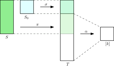
Figure 1. The construction of $\mathcal{F}(\pi)$ in Definition 5.6.1.

Fix $S_{0}\in\mathbf{FI}$, a $k\in{\mathbb{Z}}_{\geq 0}$, and a subfunctor $\mathcal{E}:\mathbf{FI}\to\mathbf{PF}$ of the functor $S\mapsto[k]^{S}$, where we require that for all $\pi\in\operatorname{Hom}\nolimits_{\mathbf{FI}}(S,T)$, $\mathcal{E}(\pi)$ is defined everywhere. Hence, by passing to count vectors as in §5.3, $\mathcal{E}$ is uniquely determined by a downward closed subset of ${\mathbb{Z}}_{\geq 0}^{k}$.

Then we define a new functor $\mathcal{F}:\mathbf{FI}\to\mathbf{PF}$ on objects by

$$\mathcal{F}(S)=\{(\sigma,\alpha)\mid\sigma\in\operatorname{Hom}\nolimits_{\mathbf{FI}}(S_{0},S),\ \alpha\in\mathcal{E}(S\setminus\operatorname{im}(\sigma))\}$$

and on a morphism $\pi\in\operatorname{Hom}\nolimits_{\mathbf{FI}}(S,T)$ as follows: for $(\sigma,\alpha)\in\mathcal{F}(T)$ we set

$$\mathcal{F}(\pi)((\sigma,\alpha)):=\begin{cases}\text{undefined if $\operatorname{im}(\sigma)\not\subseteq\operatorname{im}(\pi)$; and }\\ (\sigma^{\prime},\alpha\circ\pi|_{S\setminus\operatorname{im}(\sigma^{\prime})})\text{ where }\sigma^{\prime}:=\pi^{-1}\circ\sigma\text{ otherwise.}\end{cases}$$

Figure 1 depicts all relevant maps. At the level of species (so remembering the maps $\mathcal{F}(\pi)$ only when $\pi$ is a bijection), this is an instance of a well-known construction: $\mathcal{F}$ is the product of the species that maps $S$ to its set of bijections $S_{0}\to S$ and the species that maps $S$ to $\mathcal{E}(S)$.

Next let $\sim_{S}$ be an equivalence relation on $\mathcal{F}(S)$ for each $S$, and assume that these relations satisfy the following three axioms:

Axiom (1):

if $(\sigma,\alpha)\sim_{T}(\sigma^{\prime},\alpha^{\prime})$ and $\pi\in\operatorname{Hom}\nolimits_{\mathbf{FI}}(S,T)$ has $\operatorname{im}(\pi)\supseteq\operatorname{im}(\sigma)\cup\operatorname{im}(\sigma^{\prime})$, then $\mathcal{F}(\pi)((\sigma,\alpha))\sim_{S}\mathcal{F}(\pi)((\sigma^{\prime},\alpha^{\prime}))$;

Axiom (2):

conversely, if the pairs $(\sigma,\alpha)\in\mathcal{F}(T)$, $(\sigma^{\prime\prime},\alpha^{\prime\prime})\in\mathcal{F}(S)$, and the map $\pi\in\operatorname{Hom}\nolimits_{\mathbf{FI}}(S,T)$ satisfy $\operatorname{im}(\pi)\supseteq\operatorname{im}(\sigma)$ and $\mathcal{F}(\pi)((\sigma,\alpha))\sim_{S}(\sigma^{\prime\prime},\alpha^{\prime\prime})$, then there exists a pair $(\sigma^{\prime},\alpha^{\prime})\in\mathcal{F}(T)$ with $\operatorname{im}(\sigma^{\prime})\subseteq\operatorname{im}(\pi)$ such that $(\sigma^{\prime},\alpha^{\prime})\sim_{T}(\alpha,\sigma)$ and $\mathcal{F}(\pi)((\sigma^{\prime},\alpha^{\prime}))=(\sigma^{\prime\prime},\alpha^{\prime\prime})$; and

Axiom (3):

if $(\sigma,\alpha)\sim_{T}(\sigma^{\prime},\alpha^{\prime})$ and $i,j\in T\setminus(\operatorname{im}(\sigma)\cup\operatorname{im}(\sigma^{\prime}))$, then $\alpha(i)=\alpha(j)\Leftrightarrow\alpha^{\prime}(i)=\alpha^{\prime}(j)$.

The first axiom ensures that $\mathcal{F}/\!\!\sim:S\mapsto\mathcal{F}(S)/\!\!\sim_{S}$ is a functor $\mathbf{FI}\to\mathbf{PF}$ that comes with a canonical surjective morphism $\mathcal{F}\to\mathcal{F}/\!\!\sim$ in the sense of Definition 4.1.2; in particular, this implies that $\sim_{S}$ is preserved under the symmetric group $\operatorname{Sym}(S)$ acting on $\mathcal{F}(S)$. The second and third axioms will be crucial in §5.7.

Definition 5.6.1.

A functor of the form $S\mapsto\mathcal{F}(S)/\!\!\sim_{S}$ as constructed above is called a model functor.

Remark 5.6.2.

Each elementary model functor $S\mapsto\mathcal{E}(S)/G$ is isomorphic to a model functor with $S_{0}=\emptyset$ (so that we may leave out the $\sigma$s from the pairs) and $\alpha\sim_{S}\alpha^{\prime}$ if and only if $\alpha^{\prime}\in G\alpha$. We will see that, conversely, a model functor gives rise to to certain groupoids that play the role of $G$.

We revisit Example 1.2.4 from the perspective of model functors.

Example 5.6.3.

Let $X(S)$ be the subscheme of ${\mathbb{A}}^{S}_{{\mathbb{C}}}$ defined by the equations $x_{j}^{d}-x_{l}^{d}$ for all $j,l\in S$. Set $\zeta:=e^{2\pi i/d}$. If we fix a $j_{0}\in S$, there is a bijection between irreducible components of $X(S)$ and elements of $({\mathbb{Z}}/d{\mathbb{Z}})^{S\setminus\{j_{0}\}}$, where the component corresponding to $\alpha\in({\mathbb{Z}}/d{\mathbb{Z}})^{S\setminus\{j_{0}\}}$ is that in which each $x_{j},j\neq j_{0}$, equals $\zeta^{\alpha_{j}}x_{j_{0}}$. By identifying ${\mathbb{Z}}/d{\mathbb{Z}}$ with $[d]$ in the natural manner and regarding $j_{0}$ as the image of a $\sigma\in\operatorname{Hom}\nolimits_{\mathbf{FI}}(S_{0},S)$ where $S_{0}$ is a singleton, we obtain a surjection from the functor

$$\mathcal{F}:S\mapsto\{(\sigma,\alpha)\mid\sigma\in\operatorname{Hom}\nolimits_{\mathbf{FI}}(S_{0},S),\alpha\in[d]^{S\setminus\operatorname{im}(\sigma)}\}$$

to the component functor $\mathcal{C}_{X}$. A pair $(\sigma,\alpha)$ is mapped to the same component as a pair $(\sigma^{\prime},\alpha^{\prime})$ if and only if either $(\sigma,\alpha)=(\sigma^{\prime},\alpha^{\prime})$ or else $\sigma,\sigma^{\prime}$ have distinct images $j_{0},j_{0}^{\prime}$ and for all $j\in S\setminus\{j_{0},j_{0}^{\prime}\}$ we have $\alpha^{\prime}(j)-\alpha^{\prime}(j_{0})=\alpha(j)$ and $\alpha(j)-\alpha(j^{\prime}_{0})=\alpha^{\prime}(j)$ (both in ${\mathbb{Z}}/d{\mathbb{Z}}$). This defines an equivalence relation $\sim_{S}$ satisfying Axioms (1)–(3), and $\mathcal{C}_{X}$ is isomorphic to the model functor $S\mapsto\mathcal{F}(S)/\!\!\sim_{S}$.

Remark 5.6.4.

Informally, we think of $(\sigma,\alpha)$ as a word in $[k]^{S}$ in which the letters corresponding to $\operatorname{im}(\sigma)\subseteq S$ are concealed. If $(\sigma^{\prime},\alpha^{\prime})\sim_{S}(\sigma,\alpha)$, then $(\sigma^{\prime},\alpha^{\prime})$ corresponds to a different word in which the letters corresponding to $\operatorname{im}(\sigma^{\prime})$ are concealed. Outside of $\operatorname{im}(\sigma)\cup\operatorname{im}(\sigma^{\prime})$, by Axiom (3), the two words are equal up to some permutation of $[k]$. Axioms $(1)$ and $(2)$ simply ask that these equivalent words behave well with respect to $\mathbf{FI}$-morphisms. In the next section, we will roughly speaking attempt to “discover” the information concealed in $\operatorname{im}(\sigma)$ by looking at equivalent pairs $(\sigma^{\prime},\alpha^{\prime})$ where $\operatorname{im}(\sigma^{\prime})$ does not contain $\operatorname{im}(\sigma)$.

Example 5.6.5.

Fix a finite field ${\mathbb{F}}_{q}$ and a natural number $m$. Let $S$ be a finite set. On the set of rank-$m$ matrices in ${\mathbb{F}}_{q}^{m\times S}$ act four groups:

1. $\operatorname{GL}\nolimits_{m}({\mathbb{F}}_{q})$ by row operations;

2. $\operatorname{Sym}(S)$ by permuting columns;

3. $({\mathbb{F}}_{q}^{*})^{S}$ by scaling columns; and

4. $\operatorname{Aut}\nolimits({\mathbb{F}}_{q})$ by acting on all coordinates.

Modding out only $\operatorname{GL}\nolimits_{m}({\mathbb{F}}_{q})$, we obtain the set of $m$-dimensional codes in ${\mathbb{F}}_{q}^{S}$, and two codes are called isomorphic if they are in the same orbit under $\operatorname{Sym}(S)\ltimes G(S)$, where $G(S)=\operatorname{Aut}\nolimits({\mathbb{F}}_{q})\ltimes({\mathbb{F}}_{q}^{*})^{S}$.

Let $\mathcal{N}$ be a functor $\mathbf{FI}\to\mathbf{PF}$ that assigns to $S$ a set of $m$-dimensional codes in ${\mathbb{F}}_{q}^{S}$ and to an injective map $\pi:S\to T$ the map that sends a code $C\in\mathcal{N}(T)$ to the code

$$\{v\circ\pi\mid v\in C\}\subseteq{\mathbb{F}}_{q}^{S},$$

provided that this linear space still has dimension $m$. In particular, we require that the code above is then an element of $\mathcal{N}(S)$. This implies that $\mathcal{N}(S)$ is preserved under $\operatorname{Sym}(S)$ and that $\mathcal{N}$ is closed under puncturing. Furthermore, we assume that $\mathcal{N}(S)$ is preserved under $G(S)$. To prove Theorem 1.2.8, we need to count the orbits of $\operatorname{Sym}(S)\ltimes G(S)$ on $\mathcal{N}(S)$; this is the same as the number of orbits of $\operatorname{Sym}(S)$ on $\mathcal{M}(S):=\mathcal{N}(S)/G(S)$. We will informally call the elements of $\mathcal{M}(S)$ codes, as well. This $\mathcal{M}$ is another functor $\mathbf{FI}\to\mathbf{PF}$, and we claim that it is isomorphic to a model functor.

To see this, let $k:=|{\mathbb{F}}_{q}^{m}/{\mathbb{F}}_{q}^{*}|=1+(q^{m}-1)/(q-1)$ and fix any bijection between $[k]$ and ${\mathbb{F}}_{q}^{m}/{\mathbb{F}}_{q}^{*}$ by which we identify these two sets. Also set $S_{0}:=[m]$. Now define

$$\mathcal{E}(S):=\{ \alpha\in(({\mathbb{F}}_{q})^{m}/{\mathbb{F}}_{q}^{*})^{S}\mid$$

$$\text{the row space of the matrix $(I|\alpha)\in({\mathbb{F}}_{q})^{[m]\times(S_{0}\sqcup S)}$ is in $\mathcal{N}(S_{0}\sqcup S)$}\},$$

where $(I|\alpha)$ is the $[m]\times(S_{0}\sqcup S)$-matrix which in the $[m]\times S_{0}$-block has the identity matrix $I$ and in the $[m]\times S$-block has the matrix $\alpha$. Furthermore, define $\mathcal{F}(S)$ as the set of pairs $(\sigma,\alpha)$ with $\sigma\in\operatorname{Hom}\nolimits_{\mathbf{FI}}(S_{0},S)$ and $\alpha\in\mathcal{E}(S\setminus\operatorname{im}(\sigma))$. We have a surjective morphism $\Psi:\mathcal{F}\to\mathcal{M}$ in the sense of Definition 4.1.2 that sends $(\sigma,\alpha)$ to the orbit under $G(S)$ of the row space of $(I|\alpha)\in{\mathbb{F}}_{q}^{m\times S}$, where now $I\in{\mathbb{F}}_{q}^{[m]\times\operatorname{im}(\sigma)}$ is the permutation matrix with entries $\delta_{i,\sigma^{-1}(j)}$.

We define $\sim_{S}$ on $\mathcal{F}(S)$ by $(\sigma,\alpha)\sim(\sigma^{\prime},\alpha^{\prime})$ if and only if $\Psi((\sigma,\alpha))=\Psi((\sigma^{\prime},\alpha^{\prime}))$. We need to show that this satisfies Axioms (1),(2), and (3). Axiom (1) follows from the fact that if $(\sigma,\alpha),(\sigma^{\prime},\alpha^{\prime})$ represent the same ($G(T)$-orbit of) code(s), then the same is true after puncturing this code in a coordinate outside $\operatorname{im}(\sigma)\cup\operatorname{im}(\sigma^{\prime})$. To see Axiom (2), we puncture a code $C$ represented by $(\sigma,\alpha)$ in a coordinate $i\in T\setminus\operatorname{im}(\sigma)$, and assume that the resulting code $C^{\prime}$, represented by $(\sigma,\alpha|_{T\setminus\{i\}})$, is also represented by some other pair $(\sigma^{\prime\prime},\alpha^{\prime\prime})\in\mathcal{F}(T\setminus\{i\})$. Then the projection of $C^{\prime}$ to ${\mathbb{F}}_{q}^{\operatorname{im}(\sigma^{\prime\prime})}$ is surjective, and hence the same holds for $C$, so that $C$ is also represented by a pair of the form $(\sigma^{\prime\prime},\alpha^{\prime})$. Finally, Axiom (3) says that if in the generator matrix $(I|\alpha)$ for the code $C$ represented by $(\sigma,\alpha)$ the columns labelled $i,j\in T\setminus\operatorname{im}(\sigma)$ are parallel, then the same holds for any other pair $(\sigma^{\prime},\alpha^{\prime})$ that represents $C$ and satisfies $i,j\in T\setminus\operatorname{im}(\sigma^{\prime})$—the main point here is that parallelness is preserved under field automorphisms.

5.7. A second quasi-polynomial count

We use the notation from §5.6. So $S\mapsto\mathcal{F}(S)/\!\!\sim_{S}$ is a model functor, where $\mathcal{F}(S)$ is the set of pairs $(\sigma,\alpha)$ with $\sigma\in\operatorname{Hom}\nolimits_{\mathbf{FI}}(S_{0},S)$ and $\alpha\in\mathcal{E}(S\setminus S_{0})\subseteq[k]^{S\setminus S_{0}}$, and where $\sim_{S}$ is an equivalence relation on $\mathcal{F}(S)$ that satisfies Axioms (1),(2),(3) for model functors. The following theorem and its proof are elementary, but quite subtle—indeed, this is probably the most intricate part of the paper.

Theorem 5.7.1.

Let $S\mapsto\mathcal{F}(S)/\!\!\sim_{S}$ be a model functor $\mathbf{FI}\to\mathbf{PF}$. Then there exists a quasipolynomial $f$ such that the number of $\operatorname{Sym}([n])$-orbits on $\mathcal{F}([n])/\!\!\sim_{[n]}$ equals $f(n)$ for all $n\gg 0$.

This immediately implies Theorem 1.2.8.

Proof of Theorem 1.2.8.

By Example 5.6.5, the number of length-$n$ elements in $\mathcal{C}$ is the number of $\operatorname{Sym}([n])$-orbits on $\mathcal{F}([n])/\!\!\sim_{[n]}$ for a suitable model functor. The result now follows from Theorem 5.7.1. ∎

To prove Theorem 5.7.1, we introduce the notion of sub-model functor.

Definition 5.7.2.

Suppose that we have, for each $S\in\mathbf{FI}$, a subset $\mathcal{E}^{\prime}(S)\subseteq\mathcal{E}(S)$ such that, first, for all $\pi\in\operatorname{Hom}\nolimits_{\mathbf{FI}(S,T)}$ the pull-back map $[k]^{T}\to[k]^{S}$ that maps $\mathcal{E}(T)$ into $\mathcal{E}(S)$ also maps $\mathcal{E}^{\prime}(T)$ into $\mathcal{E}^{\prime}(S)$; and second, for all $(\sigma,\alpha)\sim_{S}(\sigma^{\prime},\alpha^{\prime})\in\mathcal{F}(S)$ with $\alpha\in\mathcal{E}^{\prime}(S\setminus\operatorname{im}(\sigma))$, we also have $\alpha^{\prime}\in\mathcal{E}^{\prime}(S\setminus\operatorname{im}(\sigma^{\prime}))$. Then $S\mapsto\mathcal{F}^{\prime}(S)/\!\!\sim_{S}$, where

$$\mathcal{F}^{\prime}(S):=\{(\sigma,\alpha)\in\mathcal{F}(S)\mid\alpha\in\mathcal{E}^{\prime}(S)\}$$

and where $\sim_{S}$ stands for the restriction of $\sim_{S}$ to $\mathcal{F}^{\prime}(S)$ is a model functor called a sub-model functor of $\mathcal{F}$.

Proof of Theorem 5.7.1.

The proof of this theorem will take up the remainder of this subsection. This will involve an induction hypothesis for a sub-model functor $\mathcal{F}^{\prime}$ of $\mathcal{F}$ and the construction of a certain groupoid for the complement $\mathcal{F}\setminus\mathcal{F}^{\prime}$.

Let $M\subseteq{\mathbb{Z}}_{\geq 0}^{k}$ be the downward-closed set consisting of all the count vectors of elements in $\mathcal{E}(S)$ for $S$ running over $\mathbf{FI}$. Since, by Dickson’s lemma, the set of downward-closed sets in ${\mathbb{Z}}_{\geq 0}^{k}$ satisfies the descending chain property, we may assume that the theorem holds for all model functors whose corresponding downward set is strictly contained in $M$.

Our goal is now to find $\mathcal{E}^{\prime}(S)\subseteq\mathcal{E}(S)$ that defines a sub-model functor $\mathcal{F}^{\prime}$ of $\mathcal{F}$ such that the downward closed set $M^{\prime}$ of $\mathcal{E}^{\prime}$ is strictly contained in $M$. Then we have

$$|\mathcal{F}(S)/\!\!\sim_{S}|=|\mathcal{F}^{\prime}(S)/\!\!\sim_{S}|\ +\ |(\mathcal{F}(S)\setminus\mathcal{F}^{\prime}(S))/\!\!\sim_{S}|$$

and this equality continues to hold if we mod out the action of $\operatorname{Sym}(S)$ on the three sets in question. Hence by the induction hypothesis we are done if we can show that the number of $\operatorname{Sym}(S)$-orbits on $(\mathcal{F}(S)\setminus\mathcal{F}^{\prime}(S))/\!\!\sim_{S}$ grows quasipolynomially in $|S|$ for $|S|\gg 0$. In this induction argument, we may of course assume that $M$ is not empty—otherwise, the quasipolynomial $0$ will do.

To construct $\mathcal{E}^{\prime}$ we proceed as follows. Let

$$A:=\{I\subseteq[k]\mid\exists v\in M:v+{\mathbb{Z}}_{\geq 0}^{I}\subseteq M\};$$

here, and in the rest of the paper, we identify ${\mathbb{Z}}_{\geq 0}^{I}$ with ${\mathbb{Z}}_{\geq 0}^{I}\times\{0\}^{[k]\setminus I}\subseteq{\mathbb{Z}}_{\geq 0}^{k}$. Note that $A$ is nonempty because $M$ is. Let $I$ be an inclusion-wise maximal element of $A$ and set

$$d:=\max\left\{\sum_{l\in[k]\setminus I}v(l)\mid v+{\mathbb{Z}}_{\geq 0}^{I}\subseteq M\right\}.$$

This is well-defined, since if the sum of the entries in such $v$ at positions outside $I$ were unbounded, then $I$ would be contained in a strictly larger element of $A$. Choose $v\in M$ such that $v+{\mathbb{Z}}_{\geq 0}^{I}\subseteq M$ and $\sum_{l\in[k]\setminus I}v(l)=d$.

Lemma 5.7.3.

For $j\in{\mathbb{Z}}_{\geq 0}$, define $v_{j}:=v+j\cdot\left(\sum_{i\in I}e_{j}\right)\in M$. There exists a $j\in{\mathbb{Z}}_{\geq 0}$ such that the vectors in $M$ that are componentwise $\geq v_{j}$ are precisely the vectors in $v_{j}+{\mathbb{Z}}_{\geq 0}^{I}$; this then also holds for all larger values of $j$.

Proof.

Suppose that for every $j\in{\mathbb{Z}}_{\geq 0}$ there is a $w_{j}\in M\setminus(v_{j}+{\mathbb{Z}}_{\geq 0}^{I})$ that is componentwise $\geq v_{j}$. Then by Dickson’s lemma the sequence $w_{1}|_{[k]\setminus I},w_{2}|_{[k]\setminus I},w_{3}|_{[k]\setminus I},\ldots$ would contain an infinite subsequence, labelled by $i_{1}<i_{2}<\ldots$, that weakly increases componentwise. It follows that $w_{i_{1}}+{\mathbb{Z}}_{\geq 0}^{I}\subseteq M$ because $M$ is downward closed and the entries of $w_{i_{j}}$ labelled by $I$ diverge to infinity. Furthermore, by the choice of $w_{i_{1}}$, the sum $\sum_{l\in[k]\setminus I}w_{i_{1}}(l)$ is strictly larger than $d$, a contradiction. ∎

From now on, we will make the following assumption on $v$:

The entries $v(l)$ are $\gg 0$ for all $l\in I$.

In particular, after replacing $v$ with the $v_{j}$ from the lemma, this implies that the vectors in $M$ that are componentwise $\geq v$ are precisely the vectors in $v+{\mathbb{Z}}_{\geq 0}^{I}$. In the course of our reasoning, we will need further assumptions on how large the $v(l)$ with $l\in I$ are—to avoid technicalities, however, we make no attempt to specify a precise lower bound that works.

The set $I$ is now uniquely determined by $v$ as the set of all positions $l\in[k]$ where $v(l)$ is very large. We call it the frequent set of $v$.

Write $v=v_{0}+v_{1}$ with $v_{0}\in{\mathbb{Z}}_{\geq 0}^{[k]\setminus I}$ and $v_{1}\in{\mathbb{Z}}_{\geq 0}^{I}$. We now define $\mathcal{F}^{\prime}:\mathbf{FI}\to\mathbf{PF}$ by setting $\mathcal{F}^{\prime}(S)$ to be the set of pairs $(\sigma,\alpha)\in\mathcal{F}(S)$ for which there exists no pair $(\sigma^{\prime},\alpha^{\prime})\sim_{S}(\sigma,\alpha)$ such that the count vector of $\alpha^{\prime}$ is in $\tilde{v}+{\mathbb{Z}}_{\geq 0}^{I}$, where $\tilde{v}:=v+v_{1}=v_{0}+2v_{1}$. Notice the factor $2$; the relevance of this will become clear towards the end of the proof.

Lemma 5.7.4.

The association $S\mapsto\mathcal{F}^{\prime}(S)/\!\!\sim_{S}$ is a sub-model functor of $\mathcal{F}$.

Proof.

By definition, $\mathcal{F}^{\prime}(S)$ is a union of of $\sim_{S}$-equivalence classes, and uniquely determined by a subset $\mathcal{E}^{\prime}(S)\subseteq\mathcal{E}(S)$ of allowed second components $\alpha$. So we need only prove that $\mathcal{F}^{\prime}$ is preserved under morphisms.

Hence let $(\sigma,\alpha)\in\mathcal{F}^{\prime}(T)$, let $\pi\in\operatorname{Hom}\nolimits_{\mathbf{FI}}(S,T)$ satisfy $\operatorname{im}(\pi)\supseteq\operatorname{im}(\sigma)$, and consider $(\tilde{\sigma},\tilde{\alpha}):=\mathcal{F}(\pi)((\sigma,\alpha))$. If $(\tilde{\sigma},\tilde{\alpha})\sim_{S}(\sigma^{\prime\prime},\alpha^{\prime\prime})$ where $\alpha^{\prime\prime}$ has a count vector in $\tilde{v}+{\mathbb{Z}}_{\geq 0}^{I}$, then by Axiom (2) for model functors there exists a pair $(\sigma^{\prime},\alpha^{\prime})\sim_{T}(\sigma,\alpha)$ with $\mathcal{F}(\pi)((\sigma^{\prime},\alpha^{\prime}))=(\sigma^{\prime\prime},\alpha^{\prime\prime})$. This means that the count vector of $\alpha^{\prime}$ is an element of $M$ that is componentwise greater than or equal to the count vector of $\alpha^{\prime\prime}$ and hence, by the choice of $\tilde{v}$, the count vector of $\alpha^{\prime}$ lies in $\tilde{v}+{\mathbb{Z}}_{\geq 0}^{I}$. This contradicts the fact that $(\sigma,\alpha)\in\mathcal{F}^{\prime}(T)$. Therefore, $\mathcal{F}(\pi)((\sigma,\alpha))\in\mathcal{F}^{\prime}(S)$. ∎

Furthermore, we observe that the downward closed subset $M^{\prime}$ corresponding to $\mathcal{E}^{\prime}$ is strictly contained in $M$, since it does not contain $\tilde{v}\in M$. Hence the induction hypothesis applies to $\mathcal{F}^{\prime}$.

Our task is therefore reduced to counting the $\operatorname{Sym}(S)$-orbits on the set of $\sim_{S}$-equivalence classes on $\tilde{\mathcal{F}}(S):=\mathcal{F}(S)\setminus\mathcal{F}^{\prime}(S)$. Note that $\tilde{\mathcal{F}}$ is not a sub-model functor of $\mathcal{F}$; rather, $\tilde{\mathcal{F}}(S)$ consists of all pairs $(\sigma,\alpha)$ that are equivalent to some pair $(\sigma^{\prime},\alpha^{\prime})$ where $\alpha^{\prime}$ has a count vector in $\tilde{v}+{\mathbb{Z}}_{\geq 0}^{I}$. Before counting these, we will work for a while with the larger set $\mathcal{F}^{\prime\prime}(S)\supseteq\tilde{\mathcal{F}}(S)$ consisting of all pairs $(\sigma,\alpha)\in\mathcal{F}(S)$ that are equivalent to some pair $(\sigma^{\prime},\alpha^{\prime})$ where the count vector of $\alpha^{\prime}$ is in $v+{\mathbb{Z}}_{\geq 0}^{I}\supseteq\tilde{v}+{\mathbb{Z}}_{\geq 0}^{I}$.

For the time being, fix a pair $(\sigma,\alpha)\in\mathcal{F}^{\prime\prime}(T)$ where $\alpha$ has count vector in $v+{\mathbb{Z}}_{\geq 0}^{I}$. This implies that all elements in $I$ occur very frequently among the entries of $\alpha$, while all elements in $[k]\setminus I$ occur very infrequently; we call $I$ the frequent set of $\alpha$ and of the pair $(\sigma,\alpha)$. Now let $(\sigma^{\prime},\alpha^{\prime})\sim_{T}(\sigma,\alpha)$. Since, by Axiom (3) for model functors, the equality patterns of $\alpha^{\prime}$ and $\alpha$ agree on $T\setminus(\operatorname{im}(\sigma)\cup\operatorname{im}(\sigma^{\prime}))$, there exists a set $I^{\prime}\subseteq[k]$ of the same cardinality as $I$, and a bijection $g=g((\sigma^{\prime},\alpha^{\prime}),(\sigma,\alpha)):I\to I^{\prime}$ such that, for $i\in T\setminus(\operatorname{im}(\sigma)\cup\operatorname{im}(\sigma^{\prime}))$, we have $\alpha(i)=l\in I$ if and only if $\alpha^{\prime}(i)=g(l)$. In particular, $\alpha^{\prime}$, too, has a distinguished set $I^{\prime}\subseteq[k]$ of elements that occur very frequently among its entries, while the complement occurs very infrequently. We call $I^{\prime}$ the frequent set of $\alpha^{\prime}$.

Furthermore, if also $(\sigma^{\prime\prime},\alpha^{\prime\prime})\sim_{T}(\sigma,\alpha)$, then we have

(1) $$g((\sigma^{\prime\prime},\alpha^{\prime\prime}),(\sigma^{\prime},\alpha^{\prime}))\circ g((\sigma^{\prime},\alpha^{\prime}),(\sigma,\alpha))=g((\sigma^{\prime\prime},\alpha^{\prime\prime}),(\sigma,\alpha))$$

as a map from $I$ to the frequent set $I^{\prime\prime}$ of $\alpha^{\prime\prime}$, and we have

(2) $$g((\sigma,\alpha),(\sigma,\alpha))=\operatorname{id}_{I}.$$

Still using elements from the $\sim_{T}$-equivalence class of $(\sigma,\alpha)$, we define a relation $\equiv$ on $T$ as follows: first, $\equiv$ is reflexive, and second, for $i\neq j$ we have $i\equiv j$ if and only if there exists $(\sigma^{\prime},\alpha^{\prime})\sim_{T}(\sigma,\alpha)$ with $i,j\not\in\operatorname{im}(\sigma^{\prime})$ and $\alpha^{\prime}(i)=\alpha^{\prime}(j)\in I^{\prime}:=g((\alpha^{\prime},\sigma^{\prime}),(\alpha,\sigma))I$.

Lemma 5.7.5.

Assume that $i\equiv j$. Then $(\sigma,\alpha)\sim_{T}\mathcal{F}((i\ j))(\sigma,\alpha)$, where $(i\ j)$ is the transposition of $i$ and $j$.

Proof.

If $i=j$, then the statement is obvious. Otherwise, there exists a pair $(\sigma^{\prime},\alpha^{\prime})\sim_{T}(\sigma,\alpha)$ such that $\alpha^{\prime}$ is defined at $i$ and $j$ and takes the same value $l$ in the frequent set of $\alpha^{\prime}$. Then $\mathcal{F}((i\ j))(\sigma^{\prime},\alpha^{\prime})=(\sigma^{\prime},\alpha^{\prime})$ and by Axiom (1), $\mathcal{F}((i\ j))(\sigma,\alpha)\sim_{T}\mathcal{F}((i\ j))(\sigma^{\prime},\alpha^{\prime})=(\sigma^{\prime},\alpha^{\prime})\sim_{T}(\sigma,\alpha)$, as desired. ∎

Lemma 5.7.6.

The relation $\equiv$ is an equivalence relation on $T$.

Proof.

First note that—using Axiom (3) for model functors—if $i\neq j$ satisfy $i\equiv j$, then in fact for all $(\sigma^{\prime},\alpha^{\prime})\sim_{T}(\sigma,\alpha)$ with $i,j\in T\setminus\operatorname{im}(\sigma^{\prime})$ we have $\alpha^{\prime}(i)=\alpha^{\prime}(j)\in I^{\prime}$. Since $\equiv$ is reflexive and symmetric by definition, we only need to show transitivity. For this, assume that $i\equiv j$ and $j\equiv h$, where we may assume that $i,j,h$ are all distinct. Let $(\sigma^{\prime},\alpha^{\prime})\sim_{T}(\sigma,\alpha)$ be such that $\alpha^{\prime}(j)=\alpha^{\prime}(h)\in I^{\prime}$. Now if $\alpha^{\prime}$ is defined at $i$, then $i\equiv j$ implies that also $\alpha^{\prime}(i)=\alpha^{\prime}(j)$ so that $i\equiv h$. Assume that $\alpha^{\prime}$ is not defined at $i$. Then let $i^{\prime}\in T\setminus\{i,j,h\}$ be a position where $\alpha^{\prime}$ is defined and such that $i^{\prime}\equiv i$—this exists, because there exists a pair $(\sigma^{\prime\prime},\alpha^{\prime\prime})\sim_{T}(\sigma,\alpha)$ for which $\alpha^{\prime\prime}$ is defined at $i$ (and defined and equal at $j$); now set $l:=\alpha^{\prime\prime}(i)$, an element in the frequent set of $\alpha^{\prime\prime}$, and take for $i^{\prime}$ any element from $((\alpha^{\prime\prime})^{-1}(l))\setminus\{i,j,h\}$. Then by Lemma 5.7.5 we have $(\sigma^{\prime},\alpha^{\prime})\sim_{T}\mathcal{F}((i\ i^{\prime}))(\sigma^{\prime},\alpha^{\prime})$ and the latter element is defined at $i,j,h$. This proves transitivity. ∎

So for all elements $(\sigma^{\prime},\alpha^{\prime})$ in the $\sim_{T}$-equivalence class of $(\sigma,\alpha)$ we have the same, well-defined equivalence relation $\equiv$ on $T$. Let $T_{1}\subseteq T$ be the set of elements that form a singleton class; we call $T_{1}$ the core of (the $\sim_{T}$-equivalence class of) $(\sigma,\alpha)$. Note that $T_{1}=T_{10}\sqcup T_{11}$ where $T_{10}$ is the set of those positions in $T$ that are in $\operatorname{im}(\sigma^{\prime})$ for all $(\sigma^{\prime},\alpha^{\prime})\sim_{T}(\sigma,\alpha)$ and $T_{11}$ is the set of elements that are in $(\alpha^{\prime})^{-1}([k]\setminus I^{\prime})$ for some $(\sigma^{\prime},\alpha^{\prime})\sim_{T}(\sigma,\alpha)$ and $I^{\prime}=g((\sigma^{\prime},\alpha^{\prime}),(\sigma,\alpha))I$. We have $T_{10}\subseteq\operatorname{im}(\sigma)$ and also $T_{11}\subseteq\operatorname{im}(\sigma)\cup\alpha^{-1}([k]\setminus I)$; in particular, $|T_{1}|$ is bounded from above by $|S_{0}|+|\alpha^{-1}([k]\setminus I)|=|S_{0}|+d$, where $d$ was the number used in the construction of $v\in M$.

The same reasoning applies to any element $(\sigma,\alpha)\in\mathcal{F}^{\prime\prime}(T)$: it unambiguously determines a subset $J\subseteq[k]$ (the frequent set of $\alpha$) of cardinality $|J|=|I|$ and a subset $T_{1}\subseteq T$ of some bounded size (the core of the pair), as well as a surjection $\tau:T\setminus T_{1}\to J$ defined by $\tau(i)=l$ if and only if there exists a $(\alpha^{\prime},\sigma^{\prime})\sim_{T}(\alpha,\sigma)$ with $\alpha^{\prime}$ defined at $i$ and $\alpha^{\prime}(i)=g((\alpha^{\prime},\sigma^{\prime}),(\alpha,\sigma))(l)$; and this surjection only has large fibres. Furthermore, passing to another element of the $\sim_{T}$-equivalence class, the core $T_{1}$ remains the same, $J$ is acted upon by a bijection $g$ to yield a $J^{\prime}$, and $\tau$ is composed with that same bijection. We now determine how certain morphisms transform the data $J,T_{1},\tau$.

Lemma 5.7.7.

Let $\pi\in\operatorname{Hom}\nolimits_{\mathbf{FI}}(S,T)$ be such that $\operatorname{im}(\pi)$ contains the core $T_{1}\subseteq T$ of (the $\sim_{T}$-equivalence class of) $(\sigma,\alpha)$, and assume that $(\tilde{\sigma},\tilde{\alpha}):=\mathcal{F}(\pi)((\sigma,\alpha))$ lies in $\mathcal{F}^{\prime\prime}(S)$. Then the frequent set of $\tilde{\alpha}$ equals the frequent set $J$ of $\alpha$, the core $S_{1}\subseteq S$ of $(\tilde{\sigma},\tilde{\alpha})$ equals $\pi^{-1}(T_{1})$, and the surjection $\tilde{\tau}:S\setminus S_{1}\to J$ determined by $(\tilde{\sigma},\tilde{\alpha})$ is the map $\tau\circ(\pi|_{S\setminus S_{1}})$ where $\tau:T\setminus T_{1}\to J$ is the surjection determined by $(\sigma,\alpha)$.

Proof.

That the frequent set $J$ remains unchanged is immediate: the elements that appear frequently in $\tilde{\alpha}$ also appear frequently in $\alpha$ and vice versa.

For the statement about the core, it suffices to show that distinct $i,j\in S$ satisfy $i\equiv j$ in the equivalence relation on $S$ defined by $(\tilde{\sigma},\tilde{\alpha})$ if and only if $\pi(i)\equiv\pi(j)$ in the equivalence relation on $T$ defined by $(\sigma,\alpha)$.

Let $i,j\in S$ be distinct and assume $i\equiv j$, so that there exists a pair $(\tilde{\sigma}^{\prime},\tilde{\alpha}^{\prime})\sim_{S}(\tilde{\sigma},\tilde{\alpha})$ with $\tilde{\alpha}^{\prime}(i)=\tilde{\alpha}^{\prime}(j)\in J$. By Axiom (2) there exists a pair $(\sigma^{\prime},\alpha^{\prime})\sim_{T}(\sigma,\alpha)$ with $\mathcal{F}(\pi)((\sigma^{\prime},\alpha^{\prime}))=(\tilde{\sigma}^{\prime},\tilde{\alpha}^{\prime})$, and we find that $\alpha^{\prime}(\pi(i))=\alpha^{\prime}(\pi(j))\in J$, so $\pi(i)\equiv\pi(j)$.

Conversely, let $i,j\in S$ be distinct and assume that $\pi(i)\equiv\pi(j)$, so there exists a pair $(\sigma^{\prime},\alpha^{\prime})\sim_{T}(\sigma,\alpha)$ with $\alpha^{\prime}(\pi(i))=\alpha^{\prime}(\pi(j))\in J$. Since $\operatorname{im}(\pi)$ contains $T_{1}$, it contains all elements of $\operatorname{im}(\sigma^{\prime})\cap T_{1}$. Using Lemma 5.7.5 we may apply transpositions $\mathcal{F}((h\ h^{\prime}))$ to $(\sigma^{\prime},\alpha^{\prime})$ for all $h\in\operatorname{im}(\sigma)\setminus\operatorname{im}(\pi)\subseteq T\setminus T_{1}$, where the $h^{\prime}\equiv h$ are all chosen distinct, disjoint from $\operatorname{im}(\sigma)$ and from $\{i,j\}$, and inside $\operatorname{im}(\pi)\setminus T_{1}$, to arrive at a $(\sigma^{\prime\prime},\alpha^{\prime\prime})\sim_{T}(\alpha^{\prime},\alpha^{\prime})$ still satisfying $\alpha^{\prime\prime}(\pi(i))=\alpha^{\prime\prime}(\pi(j))$ and now also satisfying $\operatorname{im}(\sigma^{\prime\prime})\subseteq\operatorname{im}(\pi)$. So we may apply $\mathcal{F}(\pi)$ to $(\sigma^{\prime\prime},\alpha^{\prime\prime})$ and find that $i\equiv j$.

For the statement about $\tilde{\tau}$ let $i\in S\setminus S_{1}=S\setminus\pi^{-1}(T_{1})$. Then there exists a $(\tilde{\sigma}^{\prime},\tilde{\alpha}^{\prime})\sim_{S}(\tilde{\sigma},\tilde{\alpha})$ such that $\tilde{\alpha}^{\prime}$ is defined at $i$. By Axiom (2) there exists a $(\sigma^{\prime},\alpha^{\prime})\sim_{T}(\sigma,\alpha)$ with $\mathcal{F}(\pi)((\sigma^{\prime},\alpha^{\prime}))=(\tilde{\sigma}^{\prime},\tilde{\alpha}^{\prime})$. In particular, $\alpha^{\prime}$ is defined at $\pi(i)$ and we have $\alpha^{\prime}(\pi(i))=\tilde{\alpha}^{\prime}(i)$, so that $\tilde{\tau}(i)=\tau(\pi(i))$, as desired. ∎

A special case of the lemma is that where $S=T$, and we find that $\operatorname{Sym}(S)$ acts in the expected manner on the data consisting of the frequent set (namely, trivially) and on the core $S_{1}$ and the map $\tau$. The cardinality of the core is an invariant under this action, and also preserved under the more general morphisms of Lemma 5.7.7.

The core is a finite subset of cardinality at most $|S_{0}|+d$. For each $e\in\{0,\ldots,|S_{0}|+d\}$ let $\mathcal{F}^{\prime\prime}_{e}(S)$ be the set of elements in $\mathcal{F}^{\prime\prime}(S)$ with a core of cardinality $e$, and set $\tilde{\mathcal{F}}_{e}(S):=\tilde{\mathcal{F}}(S)\cap\mathcal{F}^{\prime\prime}_{e}(S)$. We are done once we establish that for each $e$ the set of $\operatorname{Sym}(S)$-orbits on $\tilde{\mathcal{F}}_{e}(S)/\!\!\sim_{S}$ is quasipolynomial in $|S|$ for $|S|\gg 0$.

We will decouple the core from the rest of $S$. A first justification for this is the following lemma.

Lemma 5.7.8.

The number of $\operatorname{Sym}([e]\sqcup S)$-orbits on $A:=\tilde{\mathcal{F}}_{e}([e]\sqcup S)/\!\!\sim_{[e]\sqcup S}$ equals the number of $\operatorname{Sym}([e])\times\operatorname{Sym}(S)$-orbits on the set $B$ of elements in $\tilde{\mathcal{F}}_{e}([e]\sqcup S)/\!\!\sim_{[e]\sqcup S}$ with core equal to $[e]$.

Proof.

The inclusion map $B\to A$ induces a map $B/(\operatorname{Sym}([e])\times\operatorname{Sym}(S))\to A/\operatorname{Sym}([e]\sqcup S)$. This map is surjective since the core of any element in $A$ can be moved into $[e]$ by an element of $\operatorname{Sym}([e]\sqcup S)$. To see that it is also injective, note that if $\pi\in\operatorname{Sym}([e]\sqcup S)$ and $(\sigma,\alpha),(\sigma^{\prime},\alpha^{\prime})\in B$ satisfy $\mathcal{F}(\pi)((\sigma,\alpha))=(\sigma^{\prime},\alpha^{\prime})$, then $\pi$ must preserve the common core $[e]$ of both tuples, hence $\pi\in\operatorname{Sym}([e])\times\operatorname{Sym}(S)$. ∎

Consider a pair $(\sigma,\alpha)\in\mathcal{F}^{\prime\prime}_{e}([e]\sqcup T)$ with core equal to $[e]$. To such a pair we associate the quintuple $(J,\tau,\sigma_{0},\sigma_{1},\overline{\alpha})$ determined by:

1. the frequent set $J$ of $\alpha$;

2. the surjection $\tau:T\to J$;

3. the partially defined map $\sigma_{0}:S_{0}\to[e]$, which is the restriction of $\sigma$ to $\sigma^{-1}([e])$;

4. the map $\sigma_{1}:S_{0}\setminus\operatorname{dom}(\sigma_{0})\to J$ defined by $\sigma_{1}(i)=\tau(\sigma(i))$.

5. the restriction $\overline{\alpha}$ of $\alpha$ to $[e]\setminus\operatorname{im}(\sigma)$, which takes values in $[k]\setminus J$.

The quintuple remembers everything about the pair $(\sigma,\alpha)$ except the exact values (in $T$) of $\sigma$ on $S_{0}\setminus\operatorname{dom}(\sigma_{0})$: of these values, only their equivalence classes under $\equiv$ classes are remembered; these can be read off from $\sigma_{1}$ (and $\tau$). If another pair $(\sigma^{\prime},\alpha^{\prime})\in\mathcal{F}^{\prime\prime}_{e}([e]\sqcup T)$ with core equal to $[e]$ yields the same quintuple, then $(\sigma^{\prime},\alpha^{\prime})$ differs from $(\sigma,\alpha)$ by a permutation of $T$ that permutes elements within their equivalence classes under $\equiv$. Hence, by repeatedly applying Lemma5.7.5, we find that $(\sigma^{\prime},\alpha^{\prime})\sim_{[e]\sqcup T}(\sigma,\alpha)$.

We will use the notation $\sim_{[e]\sqcup T}$ for the induced equivalence relation on such quintuples. Note that $\operatorname{Sym}([e])$ fixes ($J$ and) $\tau$, whereas $\operatorname{Sym}(T)$ fixes ($J$ and) $\sigma_{0},\sigma_{1},\overline{\alpha}$. Also note that all components of the quintuple except $\tau$ can take only finitely many different values as $T$ varies. We call $(J,\sigma_{0},\sigma_{1},\overline{\alpha})$ the quadruple determined by the quintuple (and a fortiori also determined by the pair $(\sigma,\alpha)$).

We now come to the central tool for proving quasipolynomiality; note that now we work with $\tilde{\mathcal{F}}$ instead of $\mathcal{F}^{\prime\prime}$—recall that $\tilde{\mathcal{F}}$ and its complement $\mathcal{F}^{\prime}$ were defined using $\tilde{v}=v+v_{1}=v_{0}+2v_{1}$, while $\mathcal{F}^{\prime\prime}\supseteq\tilde{\mathcal{F}}$ was defined using $v$.

Definition 5.7.9.

Let $G$ be the finite directed graphs whose vertices are all quadruples of pairs in $\tilde{\mathcal{F}}_{e}([e]\sqcup T)$ with core $[e]$, where $T$ runs through $\mathbf{FI}$, and whose arrows from one quadruple $(J,\sigma_{0},\sigma_{1},\overline{\alpha})$ to $(J^{\prime},\sigma_{0}^{\prime},\sigma_{1}^{\prime},\overline{\alpha^{\prime}})$ are all bijections $g((\sigma^{\prime},\alpha^{\prime}),(\sigma,\alpha)):J\to J^{\prime}$ coming from pairs $(\sigma^{\prime},\alpha^{\prime})\sim_{[e]\sqcup T}(\sigma,\alpha)$ in $\tilde{\mathcal{F}}_{e}([e]\sqcup T)$ with core $[e]$ and with the prescribed quadruples.

Typically, the same bijection $g$ will arise from more than one pair of pairs with the prescribed quadruples; it then only appears once as an arrow $g$ between those quadruples. The following proposition will be used below to establish that $G$ is, in fact, a groupoid.

Proposition 5.7.10.

Let $(J,\tau,\sigma_{0},\sigma_{1},\overline{\alpha})$ be the quintuple of a pair $(\sigma,\alpha)\in\tilde{\mathcal{F}}_{e}([e]\sqcup T)$ with core $[e]$ and let $g$ be an arrow in $G$ from $(J,\sigma_{0},\sigma_{1},\overline{\alpha})$ to $(J^{\prime},\sigma_{0}^{\prime},\sigma_{1}^{\prime},\overline{\alpha^{\prime}})$. Then $(J^{\prime},g\circ\tau,\sigma_{0}^{\prime},\sigma_{1}^{\prime},\overline{\alpha^{\prime}})$ is also the quintuple of some pair in $\tilde{\mathcal{F}}_{e}([e]\sqcup T)$ with core $[e]$, and that quintuple is $\sim_{[e]\sqcup T}$-equivalent to the original quintuple. Furthermore, all quintuples equivalent to the original quintuple arise in this manner.

Proof.

The last statement is immediate: such an equivalent quintuple comes from an equivalent pair $(\sigma^{\prime},\alpha^{\prime})\sim_{[e]\sqcup T}(\sigma,\alpha)$, and for the arrow we can take $g=g((\sigma^{\prime},\alpha^{\prime}),(\sigma,\alpha))$.

For the first statement, let $(\tilde{\sigma},\tilde{\alpha})\sim_{[e]\sqcup S}(\tilde{\sigma}^{\prime},\tilde{\alpha}^{\prime})$ be pairs with the given quadruples such that $g=g((\tilde{\sigma}^{\prime},\tilde{\alpha}^{\prime}),(\tilde{\sigma},\tilde{\alpha}))$.

We will replace these equivalent pairs by smaller pairs, the first of which we can relate to $(\sigma,\alpha)$ so as to apply Axiom (2). The details are as follows.

For each $l\in J$ let $m_{l}$ be the minimum of $|\alpha^{-1}(l)|$ and $|\tilde{\alpha}^{-1}(l)|$ and set $n_{l}:=|\sigma_{1}^{-1}(l)|$. Define an injection $\pi$ from $[e]\sqcup\bigsqcup_{l\in J}([m_{l}]\sqcup[n_{l}])$ to $[e]\sqcup S$ that is the identity on $[e]$, sends each $[m_{l}]$ injectively to $m_{l}$ elements in $\alpha^{-1}(l)\subseteq S$ and sends each $[n_{l}]$ bijectively to the elements in $\operatorname{im}(\tilde{\sigma})\cap S$ where $\tau$ takes the value $l$. This construction ensures that $\mathcal{F}(\pi)$ is defined at $(\tilde{\sigma},\tilde{\alpha})$. It might a priori not be defined at $(\tilde{\sigma}^{\prime},\tilde{\alpha}^{\prime})$, because $\operatorname{im}(\tilde{\sigma}^{\prime})\cap S$ might not be contained in $\operatorname{im}(\pi)$. But if it is not, then using Lemma 5.7.5 we can replace $(\tilde{\sigma}^{\prime},\tilde{\alpha}^{\prime})$ by a $\sim_{S}$-equivalent pair, with the same quadruple and with the same bijection $g:J\to J^{\prime}$, such that $\mathcal{F}(\pi)$ is defined at $(\tilde{\sigma}^{\prime},\tilde{\alpha}^{\prime})$. Now replace $(\tilde{\sigma},\tilde{\alpha})$ and $(\tilde{\sigma}^{\prime},\tilde{\alpha}^{\prime})$ by their images under $\mathcal{F}(\pi)$.

The point of distinguishing $\tilde{\mathcal{F}}$ and $\mathcal{F}^{\prime\prime}$ is that these images may not be in $\tilde{\mathcal{F}}$. The reason is that while $\tilde{v}+{\mathbb{Z}}_{\geq 0}^{I}$ is closed under the map that sends a pair $w_{1},w_{2}$ of vectors to the componentwise minimum vector $\min(w_{1},w_{2})$ defined by $\min(w_{1},w_{2})(l):=\min(w_{1}(l),w_{2}(l))$, the count vectors of pairs in $\tilde{\mathcal{F}}$ with a fixed frequent set $J$ may not quite be closed under componentwise minimum: the number of entries that $\alpha$ has in the frequent set is not quite invariant under the equivalence relations $\sim$, although it is up to a bounded difference. This is remedied by allowing the componentwise minimum to have a count vector in the bigger set $v+{\mathbb{Z}}_{\geq 0}^{I}$.

Hence the new $(\tilde{\sigma},\tilde{\alpha})$ and $(\tilde{\sigma}^{\prime},\tilde{\alpha}^{\prime})$ are in $\mathcal{F}^{\prime\prime}([e]\sqcup\bigsqcup_{l\in J}([m_{l}]\sqcup[n_{l}]))$ and are related by the same bijection $g$. Now construct similarly an injection $\pi^{\prime}:[e]\sqcup\bigsqcup_{l\in J}([m_{l}]\sqcup[n_{l}])\to[e]\sqcup T$ which is the identity on $[e]$, sends $[m_{l}]$ injectively into the set $\alpha^{-1}(l)$, and sends $[n_{l}]$ bijectively to the set of elements in $\operatorname{im}(\sigma)\cap T$ where $\tau$ takes the value $l$. Then $(\tilde{\sigma},\tilde{\alpha})=\mathcal{F}(\pi^{\prime})((\sigma,\alpha))$. Now apply Axiom (2) to find that there exists a pair $(\sigma^{\prime},\alpha^{\prime})\sim_{[e]\sqcup T}(\sigma,\alpha)$ such that $\mathcal{F}(\pi^{\prime})((\sigma^{\prime},\alpha^{\prime}))=(\tilde{\sigma}^{\prime},\tilde{\alpha}^{\prime})$. The pair $(\sigma^{\prime},\alpha^{\prime})$ has the required quintuple. Moreover, since the pair is $\sim_{[e]\sqcup T}$-equivalent to $(\sigma,\alpha)$, so are their quintuples. ∎

Proposition 5.7.11.

The finite graph $G$ is a groupoid with objects its vertices (quadruples), arrows as in Definition 5.7.9, and composition maps given by composing the bijections $g$.

Before proving this in general, we revisit Example 5.6.3.

Example 5.7.12.

Consider the functor $\mathcal{F}:\mathbf{FI}\to\mathbf{PF}$ that maps $S$ to

$$\mathcal{F}(S)=\{(\sigma,\alpha)\mid\sigma\in\operatorname{Hom}\nolimits_{\mathbf{FI}}(S_{0},S),\alpha\in[d]^{S\setminus\operatorname{im}(\sigma)}\}$$

where $S_{0}$ is a singleton and where we identify $[d]$ with ${\mathbb{Z}}/d{\mathbb{Z}}$ via $a\mapsto a+d{\mathbb{Z}}$. Let $\sim_{S}$ be as in Example 5.6.3, i.e. $(\sigma,\alpha)\sim(\sigma^{\prime},\alpha^{\prime})$ if and only if either the pairs are equal, or else $\{j_{0}\}:=\operatorname{im}(\sigma)\neq\operatorname{im}(\sigma^{\prime})=:\{j_{0}^{\prime}\}$ and for all $j\in S\setminus\{j_{0},j_{0}^{\prime}\}$ we have $\alpha^{\prime}(j)-\alpha^{\prime}(j_{0})=\alpha(j)$ and $\alpha(j)-\alpha(j_{0}^{\prime})=\alpha^{\prime}(j)$ in ${\mathbb{Z}}/d{\mathbb{Z}}$.

In this case, $I=[d]$, and $v\in[d]^{I}$ is any vector containing sufficiently many copies of each element of $[d]$. Fix a pair $(\sigma,\alpha)\in\mathcal{F}^{\prime\prime}(T)$ where $\alpha$ has count vector in $v+{\mathbb{Z}}_{\geq 0}^{I}$. Set $\{j_{0}\}:=\operatorname{im}(\sigma)$. The frequent set of $\alpha$ is $J=I=[d]$, and all equivalence classes in $T$ under $\equiv$, except possibly for that of $j_{0}$, are large, since the fibres of $\alpha$ are large.

Pick a $j_{0}^{\prime}\neq j_{0}$, let $\sigma^{\prime}$ be the map $S_{0}\to T$ with image $\{j_{0}^{\prime}\}$, and define $\alpha^{\prime}:T\setminus\{j_{0}^{\prime}\}\to[d]$ via $\alpha^{\prime}(j)=\alpha(j)$ if $j\neq j_{0},j_{0}^{\prime}$ and $\alpha^{\prime}(j_{0})=d$ (which is identified with $0+d{\mathbb{Z}}$). Then it follows that $(\sigma,\alpha)\sim_{T}(\sigma^{\prime},\alpha^{\prime})$. Since $\alpha^{\prime}$ is defined at $j_{0}$ and takes the same value $d$ at least once more (in fact, many times), we conclude that the equivalence class of $j_{0}$ under $\equiv$ is not a singleton, either. Hence the core of $(\sigma,\alpha)$ is empty.

We can now complete the quintuple of $(\alpha,\sigma)$: the partially defined map $\sigma_{0}$ from $S_{0}$ to the core $\emptyset$ is the only such map, the surjection $\tau:T\to J$ equals $\alpha$ on $T\setminus\{j_{0}\}$ and $d$ on $j_{0}$, the map $\sigma_{1}$ maps the singleton $S_{0}$ to $d$, and $\overline{\alpha}$ is the empty map $\emptyset\to\emptyset$. Note that the quadruple $(J,\sigma_{0},\sigma_{1},\overline{\alpha})$ does not depend on the particular choice of $(\sigma,\alpha)$, so the groupoid $G$ has a single object.

To determine all arrows in $G$, suppose that $(\sigma,\alpha)\sim_{T}(\sigma^{\prime\prime},\alpha^{\prime\prime})$, set $\{j_{0}^{\prime\prime}\}:=\operatorname{im}(\sigma^{\prime})$, and assume that $j_{0}^{\prime\prime}\neq j_{0}$ (otherwise we get the identity arrow). Then for any $j\in T^{\prime\prime}:=T\setminus\{j_{0},j_{0}^{\prime\prime}\}$, we have

$$\alpha^{\prime\prime}(j)-\alpha(j)=(\alpha^{\prime\prime}(j)-\alpha^{\prime\prime}(j_{0}))+(\alpha^{\prime\prime}(j_{0})-\alpha(j))=\alpha(j)+(\alpha^{\prime\prime}(j_{0})-\alpha(j))=\alpha^{\prime\prime}(j_{0})$$

so that $\alpha^{\prime\prime}|_{T^{\prime\prime}}$ is obtained from $\alpha|_{T^{\prime\prime}}$ by a coordinate-wise shift over the constant $\alpha^{\prime\prime}(j_{0})=:a$. The map $g_{(\sigma,\alpha),(\sigma^{\prime\prime},\alpha^{\prime\prime})}:[d]\to[d]$ is adding $a$ (modulo $d$). Conversely, for every choice of $\alpha^{\prime\prime}(j_{0})\in[d]={\mathbb{Z}}/d{\mathbb{Z}}$, there is a unique pair $(\sigma^{\prime\prime},\alpha^{\prime\prime})$ equivalent to $(\sigma,\alpha)$. We conclude that the groupoid $G$ is just (isomorphic to) the group ${\mathbb{Z}}/d{\mathbb{Z}}$.

Proof.

That $G$ has identity arrows follows from (2), and that all arrows are invertible follows from (1) combined with (2). It remains to check that composition is well-defined. So let $g_{1}$ be an arrow in $G$ from a vertex $q:=(J,\sigma_{0},\sigma_{1},\overline{\alpha})$ to a vertex $q^{\prime}:=(J^{\prime},\sigma_{0}^{\prime},\sigma_{1}^{\prime},\overline{\alpha^{\prime}})$, and let $g_{2}$ be an arrow in $G$ from $q^{\prime\prime}:=(J^{\prime\prime},\sigma_{0}^{\prime\prime},\sigma_{1}^{\prime\prime},\overline{\alpha^{\prime\prime}})$ to $q$. We need to show that $g_{1}\circ g_{2}$ is an arrow in $G$ from $q^{\prime\prime}$ to $q^{\prime}$. Now the existence of the arrow $g_{2}$ means that there are a finite set $T$ and pairs $(\sigma,\alpha),(\sigma^{\prime\prime},\alpha^{\prime\prime})\in\tilde{F}_{e}([e]\sqcup T)$ with core $[e]$ and quadruples $q,q^{\prime\prime}$, respectively, such that $g_{2}=g((\sigma,\alpha),(\sigma^{\prime\prime},\alpha^{\prime\prime}))$.

Let $(J,\tau,\sigma_{0},\sigma_{1},\overline{\alpha})$ be the quintuple of $(\sigma,\alpha)$. By Proposition 5.7.10, $(J^{\prime},g_{1}\circ\tau,\sigma_{0}^{\prime},\sigma_{1}^{\prime},\overline{\alpha^{\prime}})$ is the quintuple of another pair $(\sigma^{\prime},\alpha^{\prime})\in\tilde{\mathcal{F}}_{e}([e]\sqcup T)$ with core $[e]$ and $(\sigma^{\prime},\alpha^{\prime})\simeq_{[e]\sqcup T}(\sigma,\alpha)$. Then $g_{1}=g((\sigma^{\prime},\alpha^{\prime}),(\sigma,\alpha))$, and $g_{1}\circ g_{2}=g((\sigma^{\prime},\alpha^{\prime}),(\sigma^{\prime\prime},\alpha^{\prime\prime}))$ is an arrow from $q^{\prime\prime}$ to $q^{\prime}$, as desired. ∎

Consider the class of quintuples arising from pairs $(\sigma^{\prime},\alpha^{\prime})\in\tilde{\mathcal{F}}([e]\sqcup T),T\in\mathbf{FI}$ with core $[e]$. This class of quintuples comes with a natural anchor map to the objects of $G$, namely, the map that forgets $\tau$. The following says that equivalence classes of quintuples are precisely orbits under $G$.

Corollary 5.7.13.

The groupoid $G$ acts on the set of quintuples of pairs in $\tilde{\mathcal{F}}([e]\sqcup T)$ with core $[e]$, for $T$ varying through $\mathbf{FI}$, via the anchor map that sends a quintuple to its corresponding quadruple. The orbits of this action are precisely the $\sim_{[e]\sqcup T}$-equivalence classes. The action of $G$ commutes with the action of $\operatorname{Sym}(T)$.

Proof.

The action of an arrow $g:(J,\sigma_{0},\sigma_{1},\overline{\alpha})\to(J^{\prime},\sigma^{\prime}_{0},\sigma^{\prime}_{1},\overline{\alpha^{\prime}})$ on a quintuple $(J,\tau,\sigma_{0},\sigma_{1},\overline{\alpha})$ yields the quintuple $(J^{\prime},g\circ\tau,\sigma^{\prime}_{0},\sigma^{\prime}_{1},\overline{\alpha^{\prime}})$, and the axioms for a groupoid action are readily verified. The action commutes with $\pi\in\operatorname{Sym}(T)$ because $(g\circ\tau)\circ\pi=g\circ(\tau\circ\pi)$. That the $G$-orbits on quintuples coming from pairs $(\sigma,\alpha)\in\tilde{\mathcal{F}}([e]\sqcup T)$ with core $[e]$ are precisely the $\sim_{[e]\sqcup T}$-equivalence classes follows from the last statement of Proposition 5.7.10. ∎

Recall that, by Lemma 5.7.8, we need to count the elements of $\tilde{\mathcal{F}}([e]\sqcup T)$ with core $[e]$ up to $\sim_{[e]\sqcup T}$ as well as up to the action of $\operatorname{Sym}([e])\times\operatorname{Sym}(T)$. Modding out the action of $\operatorname{Sym}(T)$ is now straightforward: it just consists of replacing $\tau:T\to J$ by its count vector $u$ in ${\mathbb{Z}}_{\geq 0}^{J}$. Thus now the groupoid $G$ acts on quintuples $(J,u,\sigma_{0},\sigma_{1},\overline{\alpha})$ coming from pairs in $\tilde{\mathcal{F}}_{e}([e]\sqcup T)$ with core $[e]$, where $u$ is a vector in ${\mathbb{Z}}_{\geq 0}^{J}$. Also the group $\operatorname{Sym}([e])$ acts on such quintuples, indeed, it acts on the corresponding quadruples and fixes $u$. We need to count the quintuples up to the action of $G$ and $\operatorname{Sym}([e])$. To do so, we first observe that $\operatorname{Sym}([e])$ acts by automorphisms of $G$ on the objects of $G$: if there is an arrow $g:q\to q^{\prime}$, then there is also an arrow $\pi(q)\to\pi(q^{\prime})$ with the same label $g$, for each $\pi\in\operatorname{Sym}([e])$. To stress that this arrow has a different source and target, we write $\pi(g:q\to q^{\prime})\pi^{-1}$ for that arrow $\pi(q)\to\pi(q^{\prime})$.

We now combine these actions into that of a larger groupoid $\tilde{G}$ with the same ground set as $G$ and with arrows $q\to q^{\prime\prime}$ all pairs $(\pi,g:q\to q^{\prime})$ where $g$ is an arrow from the quadruple $q$ to some quadruple $q^{\prime}$ and $\pi\in\operatorname{Sym}([e])$ maps $q^{\prime}$ to $q^{\prime\prime}$. The composition $(\pi^{\prime},g^{\prime})\circ(\pi,g)$, where $g^{\prime}:q^{\prime\prime}\to q^{\prime\prime\prime}$ and $\pi^{\prime}(q^{\prime\prime\prime})=q^{\prime\prime\prime\prime}$, is defined as $(\pi^{\prime}\circ\pi,\pi^{-1}(g^{\prime}:q^{\prime\prime}\to q^{\prime\prime\prime})\pi\circ g)$. It is straightforward to see that $\tilde{G}$ is, indeed, a finite groupoid acting on quintuples. Now we are left to count orbits of $\tilde{G}$ on quintuples.

Proposition 5.7.14.

There exists a quasipolynomial $f$ such that, for $n\gg 0$, the number of orbits of $\tilde{G}$ on quintuples $(J,u\in{\mathbb{Z}}_{\geq 0}^{J},\sigma_{0},\sigma_{1},\overline{\alpha})$ arising from pairs $(\sigma,\alpha)\in\tilde{\mathcal{F}}_{e}([e]\sqcup[n])$ with core $[e]$ equals $f(n)$.

Proof.

Applying the orbit-counting lemma for groupoids (Lemma 5.5.1), it suffices to show that for each object of $\tilde{G}$, which is a quadruple $q=(J,\sigma_{0},\sigma_{1},\overline{\alpha})$, and for each arrow $(\pi,g):q\to q$ in $\tilde{G}$, the number of fixed points of $(\pi,g)$ on quintuples with the given quadruple $q$ is quasipolynomial for $n\gg 0$. Such a quintuple is fixed if and only if the count vector $u\in{\mathbb{Z}}_{\geq 0}^{J}$ is fixed by $g$—indeed, $\pi$ acts trivially on the count vector.

Now we figure out the structure of the set of count vectors arising from such quintuples. First, if $u$ is the count vector of a quintuple (with the fixed quadruple $q$) arising from $(\sigma,\alpha)\in\tilde{\mathcal{F}}_{e}([e]\sqcup[n])$, and if $l\in J$ and $i\in[n]$ such that $\alpha(i)=l$, then $u-e_{l}$ is the count vector of the quintuple arising from the pair $(\tilde{\sigma},\tilde{\alpha}):=\mathcal{F}(\pi)((\sigma,\alpha))$, where $\pi:[e]\sqcup[n-1]\to[e]\sqcup[n]$ is the identity on $[e]$ and increasing from $[n-1]\to[n]$ and does not hit $i$. This suggest that the set of count vectors that we are considering is downward closed. However, it may be that $(\tilde{\sigma},\tilde{\alpha})$ is in $\mathcal{F}^{\prime\prime}([e]\sqcup[n-1])\setminus\tilde{\mathcal{F}}([e]\sqcup[n-1])$.

On the other hand, if we had started with $(\sigma,\alpha)\in\mathcal{F}^{\prime\prime}([e]\sqcup[n])\setminus\tilde{\mathcal{F}}([e]\sqcup[n])$ and applied such an element $\mathcal{F}(\pi)$ to it, the result would not have been an element of $\tilde{\mathcal{F}}([e]\sqcup[n-1])$.

This shows that the set of relevant count vectors is the difference $N\setminus N^{\prime}$, where $N$ and $N^{\prime}$ are downward closed sets in ${\mathbb{Z}}_{\geq 0}^{J}$. Hence, using the Stanley decomposition as in the proof of Proposition 5.3.1, the fixed points $u$ that we are counting are the lattice points in a finite disjoint union of rational cones, each given as the intersection of a linear space (the eigenspace of $g$ in ${\mathbb{R}}^{J}$ with eigenvalue $1$) and a finite union of sets of the form $u+{\mathbb{Z}}_{\geq 0}^{J^{\prime}}$ with $J^{\prime}\subseteq J$. The number of such $u$ is a quasipolynomial in $n=\sum_{l}u(l)$ for $n\gg 0$ for each of the finitely many choices of $(\pi,g)$, hence so is their sum. ∎

This completes the proof of Theorem 5.7.1.

∎

5.8. Pre-component functors

We will see that, if $X$ is a width-one $\mathbf{FI}$-scheme of finite type over a Noetherian ring $K$, then we can cover $X(S)$ by means of closed, irreducible subsets parameterised by a finite number of model functors evaluated at $S$. Then, of course, the irreducible components of $X(S)$ are among these. But to ensure that we are neither double-counting components of $X(S)$ nor counting closed subsets that are strictly contained in components, we need to keep track of the inclusions among these closed subsets. At the combinatorial level, this is done using compatible quasi-orders.

Definition 5.8.1.

Let $a\in{\mathbb{Z}}_{\geq 0}$, for each $b\in[a]$ let $k_{b}\in{\mathbb{Z}}_{\geq 0}$ and let $S\mapsto\mathcal{F}_{b}(S)/\!\!\sim_{b,S}$ be a model functor, where $\mathcal{F}_{b}(S)$ is the set of pairs $(\sigma,\alpha)$ with $\sigma:S_{0,b}\to S$ and $\alpha\in\mathcal{E}_{b}(S)\subseteq[k_{b}]^{S}$.

Suppose that we are given, for each $S\in\mathbf{FI}$, a quasi-order $\preceq_{S}$ (i.e., a reflexive and transitive relation) on the disjoint union

$$\mathcal{F}(S):=\bigsqcup_{b=1}^{a}\mathcal{F}_{b}(S).$$

This collection of quasi-orders is called compatible if the following properties are satisfied:

Compatibility (1):

whenever $\mathcal{F}_{b}(S)\ni(\sigma,\alpha)\preceq_{S}(\sigma^{\prime},\alpha^{\prime})\in\mathcal{F}_{b^{\prime}}(S)$, we have $b\leq b^{\prime}$;

Compatibility (2):

the restriction of $\preceq_{S}$ to each $\mathcal{F}_{b}(S)$ equals the equivalence relation $\sim_{b,S}$; and

Compatibility (3):

for all $\pi\in\operatorname{Hom}\nolimits_{\mathbf{FI}}(S,T)$ and $(\sigma,\alpha)\in\mathcal{F}_{b}(T)$ and $(\sigma^{\prime},\alpha^{\prime})\in\mathcal{F}_{b^{\prime}}(T)$ with $\operatorname{im}(\pi)\supseteq\operatorname{im}(\sigma)\cup\operatorname{im}(\sigma^{\prime})$ we have

$$(\sigma,\alpha)\preceq_{T}(\sigma^{\prime},\alpha^{\prime})\Rightarrow\mathcal{F}_{b}(\pi)((\sigma,\alpha))\preceq_{S}\mathcal{F}_{b^{\prime}}(\pi)((\sigma^{\prime},\alpha^{\prime})).$$

Note that the condition that $\operatorname{im}(\pi)$ contains both $\operatorname{im}(\sigma)$ and $\operatorname{im}(\sigma^{\prime})$ implies that $\mathcal{F}_{b}(\pi)((\sigma,\alpha))$ and $\mathcal{F}_{b^{\prime}}(\pi)((\sigma^{\prime},\alpha^{\prime}))$ are both defined.

Definition 5.8.2.

In the setting of the previous definition, we introduce an equivalence relation $\sim_{S}$ on $\mathcal{F}(S)$ by $(\sigma,\alpha)\sim_{S}(\sigma^{\prime},\alpha^{\prime})$ if both $(\sigma,\alpha)\preceq_{S}(\sigma^{\prime},\alpha^{\prime})$ and $(\sigma^{\prime},\alpha^{\prime})\preceq_{S}(\sigma,\alpha)$. Note that, by the first and second axioms for pre-component functors, $(\sigma,\alpha)\in\mathcal{F}_{b}(S)$ is $\sim_{S}$-equivalent to $(\sigma^{\prime},\alpha^{\prime})\in\mathcal{F}_{b^{\prime}}(S)$ if and only if $b=b^{\prime}$ and $(\sigma,\alpha)\sim_{b,S}(\sigma^{\prime},\alpha^{\prime})$.

The quasi-order $\preceq_{S}$ induces a partial order on the set

$$\mathcal{F}(S)/\!\!\sim_{S}=\bigsqcup_{b}(\mathcal{F}_{b}(S)/\!\!\sim_{b,S})$$

of equivalence classes. We define the functor $\mathcal{C}:\mathbf{FI}\to\mathbf{PF}$ on objects by

$$\mathcal{C}(S):=\{\text{the maximal elements of }\mathcal{F}(S)/\!\!\sim_{S}\}$$

and on a morphism $\pi:S\to T$ as follows. Let $c\in\mathcal{C}(T)$ be a maximal equivalence class. If $c$ contains some element $(\sigma,\alpha)\in\mathcal{F}_{b}(T)$ at which $\mathcal{F}_{b}(\pi)$ is defined (i.e., with $\operatorname{im}(\sigma)\subseteq\operatorname{im}(\pi)$), and if, moreover, $c^{\prime}:=[\mathcal{F}_{b}(\pi)((\sigma,\alpha))]_{\sim_{S}}$ is also maximal in $\mathcal{F}(S)/\!\!\sim_{S}$, then we set $\mathcal{C}(\pi)(c):=c^{\prime}\in\mathcal{C}(S)$. By the axioms for compatible quasi-orders, this is independent of the choice of the representative $(\sigma,\alpha)$ of $c$—subject to the requirement that $\mathcal{F}_{i}(\pi)$ be defined at that representative.

A functor $\mathcal{C}:\mathbf{FI}\to\mathbf{PF}$ obtained in this manner is called a pre-component functor.

5.9. The final quasipolynomial count

We retain the notation from §5.8: for each $b\in[a]$ we have a model functor $S\mapsto\mathcal{F}_{b}(S)/\!\!\sim_{b,S}$, and on the disjoint unions $\mathcal{F}(S):=\bigsqcup_{b}\mathcal{F}_{b}(S)$ (for $S\in\mathbf{FI}$) we have compatible quasi-orders $\preceq_{S}$.

Theorem 5.9.1.

Let $\mathcal{C}$ be the pre-component functor corresponding to the data above. Then the number of $\operatorname{Sym}(S)$-orbits on $\mathcal{C}(S)$ is a quasipolynomial in $|S|$ for all $S$ with $|S|\gg 0$.

The proof requires the proof technique used in §5.7, and takes up the rest of this subsection.

Proof.

By Theorem 5.7.1, we know that the number of $\operatorname{Sym}(S)$-orbits on the disjoint union of model functors $\bigsqcup_{b}(\mathcal{F}_{b}(S)/\!\!\sim_{b,S})$ is eventually quasipolynomial in $|S|$. From this disjoint union we will remove, for each $b\in[a]$, the $\sim_{b,S}$-classes of pairs $(\sigma,\alpha)$ for which there exists a $b^{\prime}>b$ and a $(\sigma^{\prime},\alpha^{\prime})\in\mathcal{F}_{b^{\prime}}(S)$ with $(\sigma,\alpha)\preceq_{S}(\sigma^{\prime},\alpha^{\prime})$. We will see that, for a fixed $b\in[a]$, the $\operatorname{Sym}(S)$-orbits on these deletions are also counted by a quasipolynomial.

To this end, fix $b\in[a]$ and let $M\subseteq{\mathbb{Z}}_{\geq 0}^{k_{b}}$ be the downward closed subset corresponding to $\mathcal{E}_{b}$. From §5.7 we recall that, to prove that the number of $\operatorname{Sym}(S)$-orbits on $\mathcal{F}_{b}(S)/\!\!\sim_{b,S}$ is quasipolynomial in $|S|$ for $|S|\gg 0$, we performed induction on $M$ using Dickson’s lemma. We do the same here.

Lemma 5.9.2.

Fix $b\in[a]$. For $|S|\gg 0$, the number of $\operatorname{Sym}(S)$-orbits on pairs $(\sigma,\alpha)\in\mathcal{F}_{b}(S)$ that are $\preceq$ some pair $(\sigma^{\prime},\alpha^{\prime})\in\mathcal{F}_{b^{\prime}}(S)$ for some $b^{\prime}>b$ is quasipolynomial in $|S|$.

Proof.

We construct the sub-functor $\mathcal{E}_{b}^{\prime}\subseteq\mathcal{E}_{b}$ and the corresponding sub-functor $\mathcal{F}_{b}^{\prime}\subseteq\mathcal{F}_{b}$ as in §5.7, as well as the difference $\tilde{\mathcal{F}}_{b}(S):=\mathcal{F}_{b}(S)\setminus\mathcal{F}^{\prime}_{b}(S)$. By induction on $M$ using Dickson’s lemma, we may assume that the lemma holds for the sub-model functor $S\mapsto\mathcal{F}_{b}^{\prime}(S)/\!\!\sim_{b,S}$. On the other hand, in §5.7 we counted the $\operatorname{Sym}(S)$-orbits on $\tilde{\mathcal{F}}_{b}(S)/\!\!\sim_{b,S}$, for all $S$, as a finite sum of orbit counts of certain finite groupoids. More precisely, for finitely many values of a nonnegative integer $e$, we there considered the pairs $(\alpha,\sigma)\in\tilde{\mathcal{F}}_{b}([e]\sqcup S)$ with core equal to $[e]$. Each of these pairs gives rise to a quintuple $(J,u\in{\mathbb{Z}}_{\geq 0}^{J},\sigma_{0},\sigma_{1},\overline{\alpha})$ where $J\subseteq[k_{b}]$ is the frequent set of $\alpha$, and we showed that the $\operatorname{Sym}(S)$-orbits on $\sim_{b,[e]\sqcup S}$-equivalence classes of such pairs $(\alpha,\sigma)$ are in bijection with the orbits of a certain groupoid on the sum-$|S|$ level set of a difference $N\setminus N^{\prime}$ where $N,N^{\prime}\subseteq{\mathbb{Z}}_{\geq 0}^{k_{b}}$ are downward closed; this difference is where the count vector $u\in{\mathbb{Z}}_{\geq 0}^{J}\subseteq{\mathbb{Z}}_{\geq 0}^{k_{b}}$ lives.

Now suppose that $(\sigma,\alpha)\preceq_{[e]\sqcup S}(\sigma^{\prime},\alpha^{\prime})$ for some $(\sigma^{\prime},\alpha^{\prime})\in\mathcal{F}_{b^{\prime}}([e]\sqcup S)$ with $b^{\prime}>b$, and let $i\in S$ be such that $l:=\alpha(i)\in J$. If $i$ happens to be in $\operatorname{im}(\sigma)\cup\operatorname{im}(\sigma^{\prime})$, then choose $j\in S\setminus(\operatorname{im}(\sigma)\cup\operatorname{im}(\sigma^{\prime}))$ such that $\alpha(i)=\alpha(j)=l$—this can be done since $l$ appears frequently in $\alpha$ (although, to be precise, when choosing the vector $\tilde{v}$ in the construction of $\tilde{F}_{b}$, we now have to make sure that its large entries values are large even compared to the finitely many numbers $k_{b^{\prime}},b^{\prime}\in[a]$).

By Lemma 5.7.5, $(\sigma,\alpha)\sim_{b,[e]\sqcup S}(\tilde{\sigma},\tilde{\alpha}):=\mathcal{F}_{b}((i\ j))((\sigma,\alpha))$, and the axioms for compatible quasi-orders imply that $(\tilde{\sigma},\tilde{\alpha})\preceq_{[e]\sqcup S}(\tilde{\sigma}^{\prime},\tilde{\alpha}^{\prime}):=\mathcal{F}_{b^{\prime}}((i\ j))((\sigma^{\prime},\alpha^{\prime}))$. Moreover, we have achieved that $i\in S\setminus(\operatorname{im}(\tilde{\sigma})\cup\operatorname{im}(\tilde{\sigma}^{\prime}))$.

Now let $\pi:[e]\sqcup S\setminus\{i\}\to[e]\sqcup S$ be the inclusion map. Then $\mathcal{F}_{b}(\pi)$ and $\mathcal{F}_{b^{\prime}}(\pi)$ are defined at $(\tilde{\sigma},\tilde{\alpha})$ and $(\tilde{\sigma}^{\prime},\tilde{\alpha}^{\prime})$, respectively, and we have

$$\mathcal{F}_{b}(\pi)((\tilde{\sigma},\tilde{\alpha}))\preceq_{[e]\sqcup S\setminus\{i\}}\mathcal{F}_{b^{\prime}}(\pi)((\tilde{\sigma}^{\prime},\tilde{\alpha}^{\prime})).$$

The count vector in ${\mathbb{Z}}_{\geq 0}^{J}$ of the left-hand side is just $u-e_{l}$.

We conclude that the set of count vectors of quintuples corresponding to pairs in $\tilde{\mathcal{F}}_{b,e}([e]\sqcup S)$ with core $[e]$ whose $\sim_{[e]\sqcup S}$-equivalence class is not maximal in $\tilde{F}([e]\sqcup S)/\!\!\sim_{[e]\sqcup S}$ is downward-closed, or more precisely the intersection of a downward-closed set with the earlier difference $N\setminus N^{\prime}$ of downward-closed sets, hence again a difference of downward-closed subsets of ${\mathbb{Z}}_{\geq 0}^{k_{b}}$. The same orbit-counting argument with groupoids as in §5.7 applies, and shows that the number of $\operatorname{Sym}(S)$-orbits on pairs in $\tilde{\mathcal{F}}(S)$ that are not maximal in $\preceq$ is a quasipolynomial. ∎

This concludes the proof of Theorem 5.9.1.

∎

5.10. Component functors “are” pre-component functors

We are now ready to establish our main result on component functors of width-one $\mathbf{FI^{op}}$-schemes.

Theorem 5.10.1.

Let $X$ be a reduced and nice width-one affine $\mathbf{FI^{op}}$-scheme of finite type over a Noetherian ring $K$. Then there exists a pre-component functor $\mathcal{C}$ and a morphism $\varphi:\mathcal{C}\to\mathcal{C}_{X}$ such that $\varphi$ is an isomorphism at the level of species.

More precisely, there exist an $a\in{\mathbb{Z}}_{\geq 0}$, nonnegative integers $k_{b}\in{\mathbb{Z}}_{\geq 0}$ for $b\in[a]$, model functors $S\mapsto\mathcal{F}_{b}(S)/\!\!\sim_{b,S}$, a collection of compatible quasi-orders $\preceq_{S}$ on $\bigsqcup_{b}\mathcal{F}_{b}(S)$ for each $S\in\mathbf{FI}$, and maps $\varphi_{b}$ that assign to any $(\sigma,\alpha)\in\mathcal{F}_{b}(S)$ an irreducible, locally closed subset $\varphi_{b}((\sigma,\alpha))$ of $X(S)$ such that, for all $S$ and $T$,

1. $X(S)$ is the union of the sets $\varphi_{b}((\sigma,\alpha))$ for $b\in[a]$ and $(\sigma,\alpha)\in\mathcal{F}_{b}(S)$;

2. two locally closed sets $\varphi_{b}((\sigma,\alpha))$ and $\varphi_{b^{\prime}}((\sigma^{\prime},\alpha^{\prime}))$ with $(\sigma,\alpha)\in\mathcal{F}_{b}(S)$ and $(\sigma^{\prime},\alpha^{\prime})\in\mathcal{F}_{b^{\prime}}(S)$ are either equal or disjoint;

3. $\mathcal{F}_{b}(S)\ni(\sigma,\alpha)\preceq_{S}(\sigma^{\prime},\alpha^{\prime})\in\mathcal{F}_{b^{\prime}}(S)$ holds if and only if $\varphi_{b}((\sigma,\alpha))$ is contained in the Zariski closure of $\varphi_{b^{\prime}}((\sigma^{\prime},\alpha^{\prime}))$; and

4. if $(\sigma,\alpha)\in\mathcal{F}_{b}(T)$ and $\pi\in\operatorname{Hom}\nolimits_{\mathbf{FI}}(S,T)$ are such that $\operatorname{im}(\pi)\supseteq\operatorname{im}(\sigma)$, so that $(\sigma^{\prime},\alpha^{\prime}):=\mathcal{F}_{b}(\pi)((\sigma,\alpha))$ is defined, then the map $X(\pi)$ maps $\varphi_{b}((\sigma,\alpha))$ dominantly into $\varphi_{b}((\sigma^{\prime},\alpha^{\prime}))$.

The pre-component functor $\mathcal{C}$ then assigns to $S$ the equivalence classes of the maximal elements of $\preceq_{S}$, and the morphism $\varphi$ is given by restricting the $\varphi_{b}$ to these maximal elements and taking the Zariski closure.

The proof of this theorem takes up the rest of this subsection.

Proof.

Let $X=\operatorname{Spec}(B)$ be a width-one $\mathbf{FI^{op}}$-scheme of finite type over a Noetherian ring $K$. We assume that $X$ is reduced and nice. By the Shift Theorem and Proposition 3.3.1 there exist $S_{0}\in\mathbf{FI}$ and $h\in B(S_{0})$ such that $X^{\prime}:=\operatorname{Sh}_{S_{0}}X[1/h]=\operatorname{Spec}(B^{\prime})$ is of product type in the sense of Definition 3.3.2. In particular, $B^{\prime}_{0}=B(S_{0})[1/h]$ is a domain, $X^{\prime}$ is isomorphic to $S\mapsto Z^{S}$ where $Z:=X^{\prime}([1])$, and for each $S\in\mathbf{FI}$, each irreducible component of $Z^{S}$ maps dominantly into $\operatorname{Spec}(B^{\prime}_{0})$.

For an $S\in\mathbf{FI}$, let $Z(S)$ be the open subset of $X(S)$ defined by

$$Z(S):=\{p\in X(S)\mid\exists\sigma:S_{0}\to S:(\sigma h)(p)\neq 0\}.$$

Let $Y(S):=X(S)\setminus Z(S)$. Note that $Y\subsetneq X$ is a proper closed $\mathbf{FI^{op}}$-subscheme of $X(S)$, but $Z(S)$ is not (quite) functorial in $S$: for $\pi\in\operatorname{Hom}\nolimits_{\mathbf{FI}}(S,T)$ and $p\in Z(T)$ it might happen that $X(\pi)(p)$ lies in $Y(S)$ rather than in $Z(S)$.

However, if $\sigma\in\operatorname{Hom}\nolimits_{\mathbf{FI}}(S_{0},T)$ and $\pi\in\operatorname{Hom}\nolimits_{\mathbf{FI}}(S,T)$ satisfy $\operatorname{im}(\sigma)\subseteq\operatorname{im}(\pi)$, then $X(\pi)$ maps the points of $Z(T)$ where $\sigma(h)$ is nonzero to points of $Z(S)$ where $(\pi^{-1}\sigma)(h)$ is nonzero. Consequently, in spite of the fact that $Z$ is not an $\mathbf{FI^{op}}$-scheme, as in Definition 4.2.1 we associate to $Z$ the component functor $\mathcal{C}_{Z}:\mathbf{FI}\to\mathbf{PF}$ that assigns to $S$ the set of irreducible components of $Z(S)$ and to $\pi\in\operatorname{Hom}\nolimits_{\mathbf{FI}}(S,T)$ the partially defined map $\mathcal{C}_{Z}(\pi):\mathcal{C}_{Z}(T)\to\mathcal{C}_{Z}(S)$ that at a component $c\in\mathcal{C}_{Z}(T)$ is defined and takes the value $c^{\prime}\in\mathcal{C}_{Z}(S)$ if and only if $X(\pi)$ maps $c$ dominantly into $c^{\prime}$.

Now $\mathcal{C}_{X}(S)$ is the union of $\mathcal{C}_{Z}(S)$ and the components in $\mathcal{C}_{Y}(S)$ that are not contained in the closure in $X(S)$ of any component of $Z(S)$.

By Noetherian induction using Theorem 2.7.1, we may assume that Theorem 5.10.1 holds for $Y\subsetneq X$, that is, there exists a morphism $\varphi$ from a pre-component functor $\mathcal{C}_{1}$ to $\mathcal{C}_{Y}$ that is an isomorphism at the level of species, and $\mathcal{C}_{1}$ is constructed from model functors $S\mapsto\mathcal{F}_{b}(S)/\!\!\sim_{b,S},b\in[a]$ and a collection of compatible quasi-orders $\preceq_{S},S\in\mathbf{FI}$, while $\varphi$ is constructed from maps $\varphi_{b}$ that assign (disjoint or equal) locally closed subsets in $Y(S)$ to pairs $(\sigma,\alpha)\in\mathcal{F}_{b}(S),b\in[a]$.

We now construct a model functor $\mathcal{C}_{2}$ and a morphism $\mathcal{C}_{2}\to\mathcal{C}_{Z}$ that is an isomorphism at the level of species.

Let $L$ be the fraction field of $B^{\prime}_{0}$ and let $X^{\prime}_{L}$ be the base change of $X^{\prime}$ to $L$. Since every irreducible component of $X^{\prime}(S)$ maps dominantly into $\operatorname{Spec}(B^{\prime}_{0})$, the morphism $\mathcal{C}_{X^{\prime}_{L}}\to\mathcal{C}_{X^{\prime}}$ is an isomorphism. So for each $S\in\mathbf{FI}$, the irreducible components of $X^{\prime}_{L}(S)$ are in bijection with the irreducible components of $X(S_{0}\sqcup S)[1/h]\subseteq Z(S_{0}\sqcup S)$. Consequently, for each injection $\sigma:S_{0}\to S$ we now have an injective map

(3) $$\{\text{irreducible components of $X^{\prime}_{L}(S\setminus\operatorname{im}(\sigma))$}\}\to\mathcal{C}_{Z}(S),\quad c\mapsto X(\tilde{\sigma})(c)$$

where $\tilde{\sigma}:S\to S_{0}\sqcup(S\setminus\operatorname{im}(\sigma))$ is the bijection that equals $\sigma^{-1}$ on $\operatorname{im}(\sigma)$ and the identity on $S\setminus\operatorname{im}(\sigma)$. The image of this injective map consists precisely of the irreducible components of $Z(S)$ on which $\sigma(h)$ is not identically zero. As we vary $\sigma$, we thus obtain all irreducible components of $Z(S)$, indeed typically multiple times.

Let $\overline{L}$ be a separable closure of $L$, and let $X^{\prime}_{\overline{L}}$ be the base change of $X^{\prime}$ to $\overline{L}$. Now we have a surjective morphism $\mathcal{C}_{X^{\prime}_{\overline{L}}}\to\mathcal{C}_{X^{\prime}_{L}}$ whose fibres are Galois orbits. More precisely, let $C_{1},\ldots,C_{k}$ be the irreducible components of $X^{\prime}_{\overline{L}}([1])=Z_{\overline{L}}$, and let $G$ be the image of the Galois group $\mathrm{Gal}(\overline{L}/L)$ in $\operatorname{Sym}([k])$ through its action on the components $C_{1},\ldots,C_{k}$. Then, as we have seen in §5.4, $\mathcal{C}_{X^{\prime}_{\overline{L}}}$ is isomorphic to the functor $S\mapsto\mathcal{E}(S):=[k]^{S}$. Furthermore, $\mathcal{C}_{X^{\prime}}\cong\mathcal{C}_{X^{\prime}_{L}}$ is isomorphic to the elementary model functor $S\mapsto\mathcal{E}(S)/G$.

Now we construct the functor $\mathcal{F}:\mathbf{FI}\to\mathbf{PF}$ by

$$\mathcal{F}(S):=\{(\sigma,\alpha)\mid\sigma:S_{0}\to S,\alpha\in\mathcal{E}(S\setminus\operatorname{im}(\sigma))\}.$$

Then, by the above, we have a surjective morphism

$$\Psi:\mathcal{F}\to\mathcal{C}_{Z};$$

concretely, $\Psi(S)$ takes $(\sigma,\alpha)\in\mathcal{F}(S)$, computes the component of $X^{\prime}_{\overline{L}}(S\setminus\operatorname{im}(\sigma))$ corresponding to $\alpha$, its image in $\mathcal{C}_{X^{\prime}_{L}}(S\setminus\operatorname{im}(\sigma))$ (modding out the Galois group), and then applies the map (3). To simplify notation, we will write $\Psi((\sigma,\alpha))$ instead of $\Psi(S)((\sigma,\alpha))$.

This surjection is by no means a bijection: even ignoring the Galois groups for a moment, on the left we have pairs of a component in $Z(S)$ and a specified $\sigma:S_{0}\to S$ such that $\sigma(h)$ is not identically zero on that component; and on the right we just have components of $Z(S)$. A single component of $Z(S)$ may admit many different such maps $\sigma$. We therefore introduce an equivalence relation $\sim_{S}$ on $\mathcal{F}(S)$ by $(\sigma,\alpha)\sim_{S}(\sigma^{\prime},\alpha^{\prime}):\Leftrightarrow\Psi((\sigma,\alpha))=\Psi((\sigma^{\prime},\alpha^{\prime}))$. In text we will sometimes opress the $S$ and say that $(\sigma,\alpha)$ is equivalent to $(\sigma^{\prime},\alpha^{\prime})$.

We will prove that the equivalence relation $\sim_{S}$ satisfies the axioms in the definition of a model functor (§5.6).

Lemma 5.10.2.

Suppose that $\mathcal{F}(T)\ni(\sigma,\alpha)\sim_{T}(\sigma^{\prime},\alpha^{\prime})\in\mathcal{F}(T)$ and let $\pi\in\operatorname{Hom}\nolimits_{\mathbf{FI}}(S,T)$ with $\operatorname{im}(\pi)\supseteq\operatorname{im}(\sigma)\cup\operatorname{im}(\sigma^{\prime})$. Then

$$\mathcal{F}(\pi)((\sigma,\alpha))\sim_{S}\mathcal{F}(\pi)((\sigma^{\prime},\alpha^{\prime}))$$

holds.

Proof.

The assumptions assert that $\Psi((\sigma,\alpha))=\Psi((\sigma^{\prime},\alpha^{\prime}))$ and that $\mathcal{C}_{Z}(\pi)$ is defined at this component of $Z(T)$. By construction, we have

$$\Psi(\mathcal{F}(\pi)((\sigma,\alpha)))=\mathcal{C}_{Z}(\pi)(\Psi((\sigma,\alpha)))=\mathcal{C}_{Z}(\pi)(\Psi((\sigma^{\prime},\alpha^{\prime})))=\Psi(\mathcal{F}(\pi)((\sigma^{\prime},\alpha^{\prime}))),$$

so that $\mathcal{F}(\pi)((\sigma,\alpha))\sim_{S}\mathcal{F}(\pi)((\sigma^{\prime},\alpha^{\prime}))$, as desired. ∎

This lemma establishes Axiom (1) for the equivalence relations $\sim_{S}$. We continue with Axiom (2).

Lemma 5.10.3.

Let $(\sigma,\alpha)\in\mathcal{F}(T)$ and let $\pi\in\operatorname{Hom}\nolimits_{\mathbf{FI}}(S,T)$ satisfy $\operatorname{im}(\pi)\supseteq\operatorname{im}(\sigma)$. Assume that $\mathcal{F}(\pi)((\sigma,\alpha))\sim_{S}(\sigma^{\prime\prime},\alpha^{\prime\prime})\in\mathcal{F}(S)$. Set $\sigma^{\prime}:=\pi\circ\sigma^{\prime\prime}$. Then there exists an $\alpha^{\prime}\in\mathcal{E}(T)$ such that $(\sigma^{\prime},\alpha^{\prime})$ lies in $\mathcal{F}(T)$, is $\sim_{T}$-equivalent to $(\sigma,\alpha)$, and satisfies $\mathcal{F}(\pi)((\sigma^{\prime},\alpha^{\prime}))=(\sigma^{\prime\prime},\alpha^{\prime\prime})$.

Proof.

Let $C:=\Psi((\sigma,\alpha))$ be the corresponding component of $Z(T)$ and $D$ its image in $Z(S)$ under $X(\pi)$. The fact that $\mathcal{F}(\pi)((\sigma,\alpha))\sim_{S}(\sigma^{\prime\prime},\alpha^{\prime\prime})\in\mathcal{F}(S)$ implies that $\sigma^{\prime\prime}(h)$ is not identically zero on $D$. Then $\sigma^{\prime}(h)=\pi(\sigma^{\prime\prime}(h))$ is not identically zero on $C$, and hence $C=\Psi((\sigma^{\prime},\tilde{\alpha}^{\prime}))$ for a suitable $\tilde{\alpha}^{\prime}\in\mathcal{E}(T)$. Then $\mathcal{F}(\pi)((\sigma^{\prime},\tilde{\alpha}^{\prime}))=(\sigma^{\prime\prime},\tilde{\alpha}^{\prime\prime})$ for $\tilde{\alpha}^{\prime\prime}:=\tilde{\alpha}^{\prime}\circ\pi|_{S\setminus\operatorname{im}(\sigma^{\prime\prime})}$ and we have $(\sigma^{\prime\prime},\tilde{\alpha}^{\prime\prime})\ \sim_{S}(\sigma^{\prime\prime},\alpha^{\prime\prime})$. Since the first component $\sigma^{\prime\prime}$ of these pairs is the same, it follows that $\alpha^{\prime\prime}=g\tilde{\alpha}^{\prime\prime}$ for some $g\in G$. Now set $\alpha^{\prime}:=g\tilde{\alpha}^{\prime}$. As the action of $G$ commutes with $\mathcal{F}(\pi)$, we have $(\sigma^{\prime\prime},\alpha^{\prime\prime})=\mathcal{F}(\pi)((\sigma^{\prime},\alpha^{\prime}))$, and since $\Psi((\sigma^{\prime},\alpha^{\prime}))=C$, we have $(\sigma^{\prime},\alpha^{\prime})\sim_{T}(\sigma,\alpha)$. ∎

Next, we extablish Axiom (3) for model functors.

Lemma 5.10.4.

Assume that $(\sigma,\alpha)\in\mathcal{F}(T)$ is $\sim_{T}$-equivalent to $(\sigma^{\prime},\alpha^{\prime})\in\mathcal{F}(T)$. Then for all all $i,j\in T\setminus(\operatorname{im}(\sigma)\cup\operatorname{im}(\sigma^{\prime}))$ we have

$$\alpha(i)=\alpha(j)\Leftrightarrow\alpha^{\prime}(i)=\alpha^{\prime}(j).$$

Proof.

Set $C:=\Psi((\sigma,\alpha))=\Psi((\sigma^{\prime},\alpha^{\prime}))$, an irreducible component of $Z(T)$. Set $D:=X(\operatorname{im}(\sigma))[1/(\sigma h)]$, and note that the inclusion $\operatorname{im}(\sigma)\to T$ yields a dominant morphism $C\to D$. Similarly, the inclusion $\operatorname{im}(\sigma^{\prime})\to T$ yields a dominant morphism $C\to D^{\prime}:=X(\operatorname{im}(\sigma^{\prime}))[1/(\sigma^{\prime}h)]$.

Furthermore, let $\tilde{D}$ the image of $C$ in $X(\operatorname{im}(\sigma)\cup\operatorname{im}(\sigma^{\prime}))[1/(\sigma h),1/(\sigma^{\prime}h)]$ under the morphism coming from the inclusion $\operatorname{im}(\sigma)\cup\operatorname{im}(\sigma^{\prime})\to T$. Note that $X(\sigma)$ maps $D$ isomorphically onto $\operatorname{Spec}(B_{0}^{\prime})$ and $X(\sigma^{\prime})$ maps $D^{\prime}$ isomorphically onto $\operatorname{Spec}(B_{0}^{\prime})$, and that $\tilde{D}$ maps dominantly into $D$ and into $D^{\prime}$.

Now let $M$ be the field of rational functions on $D$, and $M^{\prime}$ the field of rational functions on $D^{\prime}$. Note that $\sigma$ and $\sigma^{\prime}$ give rise to isomorphisms from $L$ to $M$ and $M^{\prime}$, respectively. We extend these isomorphisms to isomorphisms from $\overline{L}$ to separable closures $\overline{M}$ and $\overline{M^{\prime}}$ of $M,M^{\prime}$. This yields isomorphisms from $\mathrm{Gal}(\overline{L}/L)$ to the Galois groups $\mathrm{Gal}(\overline{M}/M)$ and $\mathrm{Gal}(\overline{M^{\prime}}/M)$.

The base change $C_{\overline{M}}$ equals

$$\bigcup_{\beta\in G\alpha}\prod_{i\in T\setminus\operatorname{im}(\sigma)}C_{\beta_{i}};$$

here the product is over $\overline{M}$ and $C_{\beta_{i}}$ is regarded as a variety over $\overline{M}$ via the isomorphism $\overline{L}\to\overline{M}$; and similarly for $(\sigma^{\prime},\alpha^{\prime})$. The base change $\tilde{D}_{\overline{M}}$ splits as a similar union of products, but now over $\beta\in G\alpha|_{\operatorname{im}(\sigma^{\prime})\setminus\operatorname{im}(\sigma)}$.

Let $\tilde{M}\supseteq M\cup M^{\prime}$ be the field of rational functions of $\tilde{D}$, and let $\overline{\tilde{M}}\supseteq\overline{M}\cup\overline{M^{\prime}}$ be a separable closure of $\tilde{M}$. The components of the base change $C_{\overline{\tilde{M}}}$ can then be computed in two different ways: by first doing a base change to $\overline{M}$ or by first doing a base change to $\overline{M^{\prime}}$. For the first route, we have to analyse what happens to the product over $\overline{M}$

$$\prod_{i\in T\setminus\operatorname{im}(\sigma)}C_{\beta_{i}}$$

when doing a base change to $\overline{\tilde{M}}$. Write this product as $V\times_{\overline{M}}W$, where $V$ is the product over all $i\in\operatorname{im}(\sigma^{\prime})\setminus\operatorname{im}(\sigma)$, and hence an irreducible component of $\tilde{D}_{\overline{M}}$; and $W$ is the product over all $i\in T\setminus(\operatorname{im}(\sigma)\cup\operatorname{im}(\sigma^{\prime}))$. The function field $\tilde{M}$ of the irreducible $M$-scheme $\tilde{D}$ embeds into the function field of any component of $\tilde{D}_{\overline{M}}$, hence in particular into $\overline{M}(V)$, and this field extension is algebraic, so that $\overline{\tilde{M}}\cong\overline{\overline{M}(V)}$. So the base change to $\overline{\tilde{M}}$ of the product $V\times_{\overline{M}}W$ is just the base change of $W$ over the separably closed field $\overline{M}$ with the field extension $\overline{\overline{M}(V)}$ and hence still irreducible (e.g. by [Sta20, Tag 020J]).

Summarising, we obtain a bijection from the irreducible components of $C_{\overline{M}}$, which are labelled by elements of $G\alpha$, to the irreducible components of $C_{\overline{\tilde{M}}}$, and that bijection is evidently $\operatorname{Sym}(T\setminus(\operatorname{im}(\sigma)\cup\operatorname{im}(\sigma^{\prime})))$-equivariant. As a consequence, for $i,j\in T\setminus(\operatorname{im}(\sigma)\cup\operatorname{im}(\sigma^{\prime}))$ we have $\alpha(i)=\alpha(j)$ if and only if the transposition $(i\ j)$ preserves some (and then each) component in $C_{\overline{M}}$, if and only if that transposition preserves some (and then each) component in $C_{\overline{\tilde{M}}}$.

Similarly, we obtain a bijection from the irreducible components of $C_{\overline{M^{\prime}}}$, which are labelled by elements of $G\alpha^{\prime}$, to the irreducible components of $C_{\overline{\tilde{M}}}$, with the same remark about compatibility with the transposition $(i\ j)$. Combining these results, we find that for $i,j\in T\setminus(\operatorname{im}(\sigma)\cup\operatorname{im}(\sigma^{\prime}))$ we have $\alpha(i)=\alpha(j)$ if and only if $\alpha^{\prime}(i)=\alpha^{\prime}(j)$. ∎

We have now concluded the proof that $\mathcal{C}_{2}:S\mapsto\mathcal{F}(S)/\!\!\sim_{S}$ is a model functor; and by construction, the map $\mathcal{C}_{2}\to\mathcal{C}_{Z}$ induced by $\Psi$ is a morphism that is an isomorphism at the level of species.

Finally, we combine the pre-component functor $\mathcal{C}_{1}$ (mapping onto $\mathcal{C}_{Y}$) and the model functor $\mathcal{C}_{2}$ (mapping onto $\mathcal{C}_{Z}$) as follows. Recall that $\mathcal{C}_{1}$ is constructed by taking the equivalence classes of maximal elements in $\bigsqcup_{b\in[a]}\mathcal{F}_{b}(S)$. We now set $\mathcal{F}_{a+1}:=\mathcal{F}(S)$, and we extend $\preceq_{S}$ from $\bigsqcup_{b\in[a]}\mathcal{F}_{b}(S)$ to $\bigsqcup_{b\in[a+1]}\mathcal{F}_{b}(S)$ by setting it equal to $\sim_{S}$ on $\mathcal{F}_{a+1}(S)=\mathcal{F}(S)$, and for $(\sigma,\alpha)\in\mathcal{F}_{b}(S)$ with $b\leq a$ and $(\sigma^{\prime},\alpha^{\prime})\in\mathcal{F}_{a+1}(S)$ we set $(\sigma,\alpha)\preceq_{S}(\sigma^{\prime},\alpha^{\prime})$ if and only if the irreducible locally closed subset $\varphi_{b}((\sigma,\alpha))$ of $Y(S)$ is contained in the Zariski closure of the irreducible component $\varphi_{a+1}((\sigma^{\prime},\alpha^{\prime})):=\Psi((\sigma^{\prime},\alpha^{\prime}))$ of $Z(S)$. Properties (1)–(4) in Theorem 5.10.1 are then straightforward, and so are the properties Compatibility (1) and (2) from the definition of pre-component functors. For instance, Compatibility (1) follows from the fact that no component of $Z(S)$ can be contained in $Y(S)$.

Regarding Compatibility (3): for $b=b^{\prime}=a+1$ this is just Axiom (1), verified in Lemma 5.10.2; and for $b\leq a,b^{\prime}=a+1$ it follows from the simple fact that if the irreducible locally closed set $\varphi_{b}((\sigma,\alpha))$ in $Y(T)$ is contained in the Zariski closure of the component $\Psi((\sigma^{\prime},\alpha^{\prime}))$ of $Z(T)$, then the same holds for their projections in $Y(S)$ and $Z(S)$, respectively, along the map $X(\pi)$.

With this quasi-order, the pre-component functor $\mathcal{C}_{1}$ and the model functor $\mathcal{C}_{2}$ are combined into a pre-component functor $\mathcal{C}_{3}$ with an obvious morphism to $\mathcal{C}_{X}$ that is an isomorphism at the level of species. ∎

5.11. Proof of the Main Theorem

Proof of Theorem 1.1.1.

Before the Main Theorem we introduced $\mathbf{FI^{op}}$-schemes slightly differently than we do in §2, but the two definitions are equivalent via Remark 2.2.3. So we may assume that $X$ is a width-one $\mathbf{FI^{op}}$-scheme of finite type over a Noetherian ring $K$ in the sense of §2. Furthermore, since the Main Theorem only makes a statement about the underlying topological space of $X([n])$ for $n\gg 0$, we may assume that $X$ is both nice and reduced.

By Theorem 5.10.1, the component functor $\mathcal{C}_{X}$ of $X$ is, at the level of species, isomorphic to a pre-component functor $\mathcal{C}$. In particular, for all $S$, the number of $\operatorname{Sym}(S)$-orbits on $\mathcal{C}_{X}(S)$ equals the number of $\operatorname{Sym}(S)$-orbits on $\mathcal{C}(S)$. By Theorem 5.9.1, this number is a quasipolynomial in $|S|$ for all sufficiently large $S$. This proves the Main Theorem and concludes our paper. ∎

References

- [AH07] Matthias Aschenbrenner and Christopher J. Hillar. Finite generation of symmetric ideals. Trans. Am. Math. Soc., 359(11):5171–5192, 2007.
- [BD11] Andries E. Brouwer and Jan Draisma. Equivariant Gröbner bases and the two-factor model. Math. Comput., 80:1123–1133, 2011.
-
[BDES21]
Arthur Bik, Jan Draisma, Rob H. Eggermont, and Andrew Snowden.
The geometry of polynomial representations.
Int. Math. Res. Not., 2021.
To appear,
arXiv:2105.12621. - [CEF15] Thomas Church, Jordan S. Ellenberg, and Benson Farb. FI-modules: a new approach to stability for -representations. Duke Math. J., 164(9):1833–1910, 2015.
- [CEFN14] Thomas Church, Jordan S. Ellenberg, Benson Farb, and Rohit Nagpal. FI-modules over Noetherian rings. Geom. Topol., 18(5):2951–2984, 2014.
- [Coh67] Daniel E. Cohen. On the laws of a metabelian variety. J. Algebra, 5:267–273, 1967.
- [Coh87] Daniel E. Cohen. Closure relations, Buchberger’s algorithm, and polynomials in infinitely many variables. In Computation theory and logic, volume 270 of Lect. Notes Comput. Sci., pages 78–87, 1987.
- [DEKL16] Jan Draisma, Rob H. Eggermont, Robert Krone, and Anton Leykin. Noetherianity for infinite-dimensional toric varieties. Algebra & Number Theory, 9(8):1857–1880, 2016.
- [Dra10] Jan Draisma. Finiteness for the k-factor model and chirality varieties. Adv. Math., 223:243–256, 2010.
- [Dra19] Jan Draisma. Topological Noetherianity of polynomial functors. J. Am. Math. Soc., 32:691–707, 2019.
- [Eis95] David Eisenbud. Commutative Algebra. With a View toward Algebraic Geometry, volume 150 of Graduate Texts in Mathematics. Springer-Verlag, Berlin, 1995.
- [GN18] Sema Güntürkün and Uwe Nagel. Equivariant Hilbert series of monomial orbits. Proc. Am. Math. Soc., 146(6):2381–2393, 2018.
-
[HKL13]
Christopher J. Hillar, Robert Krone, and Anton Leykin.
EquivariantGB Macaulay2 package.
Webpage:
people.math.gatech.edu/~rkrone3/EquivariantGB.html, 2013. - [HS12] Christopher J. Hillar and Seth Sullivant. Finite Gröbner bases in infinite dimensional polynomial rings and applications. Adv. Math., 221:1–25, 2012.
- [JKLR20] Martina Juhnke-Kubitzke, Dinh Van Le, and Tim Römer. Asymptotic behavior of symmetric ideals: a brief survey. In Combinatorial structures in algebra and geometry. NSA 26, Constanţa, Romania, August 26 – September 1, 2018, pages 73–94. Cham: Springer, 2020.
- [Joy81] Andre Joyal. Une théorie combinatoire des séries formelles. Adv. Math., 42:1–82, 1981.
- [KLS17] Robert Krone, Anton Leykin, and Andrew Snowden. Hilbert series of symmetric ideals in infinite polynomial rings via formal languages. J. Algebra, 485:353–362, 2017.
-
[KR22]
Mario Kummer and Cordian Riener.
Equivariant algebraic and semi-algebraic geometry of infinite affine
space.
2022.
Preprint;
arXiv:2203.11921. - [Nag21] Uwe Nagel. Rationality of equivariant Hilbert series and asymptotic properties. Trans. Am. Math. Soc., 374(10):7313–7357, 2021.
- [NR17] Uwe Nagel and Tim Römer. Equivariant Hilbert series in non-Noetherian polynomial rings. J. Algebra, 486:204–245, 2017.
- [NR19] Uwe Nagel and Tim Römer. FI- and OI-modules with varying coefficients. J. Algebra, 535:286–322, 2019.
-
[NS20]
Rohit Nagpal and Andrew Snowden.
Symmetric subvarieties of infinite affine space.
2020.
Preprint,
arXiv:2011.09009. - [SS17] Steven V. Sam and Andrew Snowden. Gröbner methods for representations of combinatorial categories. J. Am. Math. Soc., 30(1):159–203, 2017.
- [Sta82] Richard P. Stanley. Linear Diophantine equations and local cohomology. Invent. Math., 68:175–193, 1982.
- [Sta97] Richard P. Stanley. Enumerative combinatorics. Vol. 1., volume 49. Cambridge: Cambridge University Press, 1997.
- [Sta20] The Stacks project authors. The stacks project. https://stacks.math.columbia.edu, 2020.
-
[VNNR18]
Dinh Van Le, Uwe Nagel, Hop D. Nguyen, and Tim Römer.
Castelnuovo-mumford regularity up to symmetry.
Int. Math. Res. Not., 2018.
to appear,
arXiv:1806.00457. - [VNNR20] Dinh Van Le, Uwe Nagel, Hop D. Nguyen, and Tim Römer. Codimension and projective dimension up to symmetry. Math. Nachr., 293(2):346–362, 2020.