Convergence of Fermionic Observables in the Massive Planar FK-Ising Model

Abstract.

We prove convergence of the 2- and 4-point fermionic observables of the FK-Ising model on simply connected domains discretised by a planar isoradial lattice in massive (near-critical) scaling limit. The former is alternatively known as a (fermionic) martingale observable (MO) for the massive interface, and in particular encapsulates boundary visit probabilties of the interface. The latter encodes connection probabilities in the 4-point alternating (generalised Dobrushin) boundary condition, whose exact convergence is then further analysed to yield crossing estimates for general boundary conditions. Notably, we obtain a massive version of the so-called Russo-Seymour-Welsh (RSW) type estimates on isoradial lattice.

These observables satisfy a massive version of s-holomorphicity [Smi10], and we develop robust techniques to exploit this condition which do not require any regularity assumption of the domain or a particular direction of perturbation. Since many other near-critical observables satisfy the same relation (cf. [BeDu12, CIM21, Par19]), these strategies are of direct use in the analysis of massive models in broader setting.

1. Introduction

Fortuin-Kasteleyn (FK) percolation, also known as the Random Cluster model [FoKa72], is one of the most well-studied models of equilibrium statistical mechanics. This is in part due to its coupling with the well-known Potts model, called Edwards-Sokal coupling (see e.g. [Gri06]). Concretely, the FK model (indexed by $q\in[1,\infty)$) is a probability measure on subsets of weighted edges (bonds) on the underlying graph, with $q=1$ case giving rise to the familiar Bernoulli bond percolation. The FK model in two dimensions shows natural duality: it has been recently proved [DGHMT16, DST17] that the model on square lattice exhibits continuous (for $q\in\left[1,4\right]$) and discontinuous (for $q>4$) phase transition at the self-dual point with constant weights $p=p_{\text{sd}}^{q}$.

In this paper, we focus our attention to the $q=2$ case (and re-purpose the letter $q$ henceforth), also known as the FK-Ising model, defined on an isoradial graph, where each face is circumscribed by a circle of a given (constant in space) radius $\delta>0$. The coupled Potts model in that case is the famed (spin-)Ising model [Len20, Isi25], which has been subject to extensive mathematical analysis dating back to Onsager’s celebrated exact solution [Ons44]. We are mainly interested in the behaviour of the model in the scaling limit, where the underlying graph becomes infinite in sequence by discretising a given simply connected domain by isoradial lattices of mesh size $\delta\downarrow 0$. This discrete setup was used in [ChSm12] to study the critical scaling limit, i.e. the model is kept at its critical (also self-dual) point. They showed that the emerging continuous regime shows certain conformal invariance as described by Conformal Field Theory ([BPZ84], see also e.g. [DMS97]): the 2-point and 4-point fermionic observables, which are deterministic functions defined on the discrete domain, converge to universal (independent of the lattice setup) holomorphic functions on the continuous domain. We show analogous convergence results for the massive scaling limit.

The massive scaling limit, roughly speaking, corresponds to studying the model with weights at some $O(\delta)$ distance from the critical ones. On the square lattice, the weights commonly scale $p=p_{\text{sd}}+m\delta$ for a given constant parameter $m>0$ (with the dual model having weights below $p_{\text{sd}}$). More generally, on isoradial graph, there is a one-parameter family of weights (naturally parametrised by the nome $q\in\left[0,1\right]$), coupled to the Z-Invariant Ising model [Bax78], which allows for explicit discrete analysis (e.g. [dT18, BdTR19]). With this choice, we observe the emergence of a massive regime in the scaling limit. As opposed to the scale invariant critical regime $(q=0$), the massive regime $(q=\frac{m\delta}{2}$) is expected to have a finite length scale $\xi\propto\frac{1}{m}$. For example, for the probability that two bulk points are connected on the square lattice in the FK-Ising model, such exponential dropoff may be derived from rigorous results on the massive spin-Ising model, which was pioneered by the miraculous discovery of the third Painlevé transcendent for the full plane correlations by Wu, McCoy, Tracy, and Barouch [WMTB76] (see also [SMJ77, PaTr83, Par19]).

Here we choose to follow the viewpoint taken by [DGP14], which in turn is inspired by the study of massive (Bernoulli) percolation in two dimensions (e.g. [Kes87, Nol08]). We consider the discrete scale (which we will refer to as characteristic length in this paper following [DuMa20]) $L_{\rho,\epsilon,q=\frac{1}{2}m\delta}$ at which the probability of crossing a rectangular box of aspect ratio $\rho>0$ drops to small but nonzero $\epsilon>0$, and show that $\delta L_{\rho,\epsilon,q=\frac{1}{2}m\delta}$ remains a finite nonzero quantity. On the square lattice, the lower bound $L_{\rho,\epsilon,q=\frac{1}{2}m\delta}\apprge\delta^{-1}$ was shown in [DGP14] by first proving the so-called Russo-Seymour-Welsh (RSW) type estimate for the model, which is in itself of fundamental interest (see [DHN11, CDH16, DLM18] for results at criticality); the upper bound was shown in the recently announced [DuMa20]. Here we derive analogous results on isoradial lattice directly from analysis of the observable, in particular the upper bound from an exact crossing estimate on any conformal quadrilateral with 4-point (generalised) Dobrushin boundary conditions.

Many recent results dealing with conformal invariance of the critical Ising model have been shown by first establishing convergence of the fermionic observables to explicit holomorphic functions (e.g. [Smi10, ChSm12, HoSm13, HoKy10, ChIz13, CHI15, GHP19, CHI21]). These results crucially exploit the discrete integrability condition known as spin, strong, or simply s-holomorphicity, first formulated in [Smi10] for the critical case. Off the critical point, the observables satisfy [BeDu12] a discretised notion of perturbed holomorphicity (Bers-Vekua equation [Ber56, Vek62, BBC16]), part of which (in the form of massive harmonicity) [DGP14] has already exploited on standard domains together with symmetries of the square lattice. On a general isoradial lattice, without analogous discrete symmetry, we are led to develop general techniques for the analysis of such massive s-holomorphic functions, along with [Par19, CIM21]. Recently Chelkak has introduced s-embeddings, proving the convergence of, e.g. 2-point observables (exactly corresponding to ours), to a critical limit in a considerably more general setup [Che18, Che20]. These approaches build on the appearance of a fermionic structure and difference identities in the discrete model, which had been noted and used variously in, e.g., [Kau49, KaCe71, Per80, PaTr83, Mer01]. See also [Pal07] for a comprehensive historical overview.

Analysis on simply connected domains with possibly rough boundary becomes especially relevant from the viewpoint of the massive scaling limit of the interface: with 2-point Dobrushin boundary condition (see Introduction), the law of the unique interface separating the wired cluster from the dual-wired cluster should tend to a massive perturbation of the critical limit, the Schramm-Loewner Evolution $SLE(16/3)$. Such convergence result is usually proved by showing the convergence of a martingale observable (which our 2-point observable serves as one) on general domains along with RSW-type estimates (see, e.g., [Smi06]): indeed, critical analogues of results discussed in this paper almost immediately implies convergence of the critical interface to $SLE(16/3)$ [CDHKS14]. In contrast, in the massive case, more analysis is presently needed for unique identification of the scaling limit, mainly due to complications in the variation analysis with respect to the domain slit by the interface. We note that similar difficulties arise in the study of massive percolation interface, whose conjectured Loewner driving function [GPS18] is rather rough and tricky to work with, despite many interesting results on any given scaling limit of the interface [NoWe09].

1.1. Discrete Setting

Isoradial Graph

The setting of our discrete model is the isoradial graph, on which the connection between discrete complex analysis and dimer and critical Ising models have been studied in, e.g., see [Mer01, ChSm12]. The relationship between the massive Ising model and the so-called massive Laplace and Dirac operators on isoradial graphs has been also made rigorous [BdTR17, dT18]. For the convenience of the interested reader, we choose to align broadly with [ChSm12, dT18] on conventions and notations.

An isoradial lattice is a planar lattice (i.e. graph tiling of $\mathbb{C}$) where each face is circumscribed by a circle of fixed radius (the mesh size) $\delta>0$. We consider finite subgraphs $G$, whose standard components we denote as follows (Figure 1L):

• the set of (primal, or black), vertices $\Gamma(G)$;

• the set of dual, or white, vertices $\Gamma^{*}(G)$ corresponding to faces of $G$, identified with the centres of their circumscribing circles;

• the dual graph $G^{*}$ is also isoradial with vertices $\Gamma(G^{*})\cong\Gamma^{*}(G)$ and faces $\Gamma^{*}(G^{*})\cong\Gamma(G)$;

• the double graph with vertices in $\Lambda(G):=\Gamma(G)\cup\Gamma^{*}(G)$ and two vertices are adjacent if and only if they are incident on $G$ has rhombic faces;

• the set of these rhombi $\lozenge(G)=\Lambda^{*}(G)$ is naturally isomorphic to the sets of primal edges, which is also in bijection with the set of dual edges $\lozenge\left(G^{*}\right)$ (perpendicular to primal edges, connecting adjacent points in $\Gamma^{*}$);

• any rhombus $z$ has the half-angle $\overline{\theta}_{z}$ formed by its primal diagonal and any of its four rhombus edges;

• the set of rhombus edges $\Upsilon(G)$ corresponding to corners of the faces in $G$;

• a corner $\xi=\left\langle uw\right\rangle$ for $u\in\Gamma,w\in\Gamma^{*}$ is given the direction $\nu(\xi):=\frac{w-u}{\left|w-u\right|}$ pointing towards the dual vertex.

We denote the corresponding full-plane sets as $\Gamma$, $\lozenge$, etc. We impose the standard assumption that there is a uniform angle bound $\eta>0$ such that all half-angles $\overline{\theta}_{z}\in\left[\eta,\frac{\pi}{2}-\eta\right]$.

Isoradial Discretisation

We paste together a finite (but asymptotically unbounded) number of rhombi in $\lozenge$ to create a simply connected polygonal domain which we identify with the underlying isoradial graph.

Specifically, we consider discretisations $\Omega^{\delta}$ of a bounded planar simply connected domain $\Omega\subset\mathbb{C}$. We refer to the boundary $\partial\Omega$ and the closure $\overline{\Omega}$ in the sense of prime ends, homeomorphic to $\partial\mathbb{D}$ under the completion of a conformal map from the unit disc $\mathbb{D}$ to $\Omega$ (see e.g. [Pom92, Section 2.4]). To speak of Dobrushin boundary conditions, we endow $\Omega$ with some marked points in $\partial\Omega$, of which we treat 2- and 4-point cases explicitly.

For the 2-point case, we consider marked points $a,b$ partitioning $\partial\Omega$ into two (open, but see Remark 5.9) segments (going counterclockwise) $\left(ab\right),\left(ba\right)$. Consider for $\delta\downarrow 0$ simply connected polygonal domains $\Omega^{\delta}$ composed of finitely many rhombi, whose boundary is an arc of alternating primal and dual vertices. We select two marked corners (rhombus edges) $a^{\delta}=\left\langle a_{\text{b}}^{\delta}a_{\text{w}}^{\delta}\right\rangle$ and $b^{\delta}=\left\langle b_{\text{b}}^{\delta}b_{\text{w}}^{\delta}\right\rangle$ on the boundary such that, travelling along the boundary counterclockwise, $a^{\delta}$ is traversed in the direction of $a_{\text{b}}^{\delta}\to a_{\text{w}}^{\delta}$, and $b^{\delta}$ is traversed in the direction of $b_{\text{w}}^{\delta}\to b_{\text{b}}^{\delta}$. We assume that $\Omega^{\delta}$ converges to $\Omega$ in the Carathéodory sense, with $a^{\delta},b^{\delta}\in\partial\Omega^{\delta}$ converging to $a,b\in\partial\Omega$ as prime ends.

Then the boundary arc $(a_{\text{w}}^{\delta}b_{\text{w}}^{\delta})$, designated free, is the path of the dual edges running from $a_{\text{w}}^{\delta}$ to $b_{\text{w}}^{\delta}$ which will be dual-wired in the model. The arc $(b_{\text{b}}^{\delta}a_{\text{b}}^{\delta})$ is wired, and is similarly the path of the primal edges running from $b_{\text{b}}^{\delta}$ to $a_{\text{b}}^{\delta}$. For conciseness, we will frequently write $(a_{\text{w}}^{\delta}b_{\text{w}}^{\delta})=(a^{\delta}b^{\delta})$, etc. The rhombi bisected by these edges form the boundary $\partial\lozenge\left(\Omega^{\delta}\right)$, and the rest in the interior form the set $\lozenge\left(\Omega^{\delta}\right)$ where the random configurations are sampled.

For the 4-point (conformal quadrilateral) case, we simply consider two more corners $c^{\delta},d^{\delta}\to c,d$ along $\left(b^{\delta}a^{\delta}\right)$ such that they are respectively oriented in the same direction as $a^{\delta},b^{\delta}$. Accordingly, the arcs $\left(a_{\text{w}}^{\delta}b_{\text{w}}^{\delta}\right),\left(c_{\text{w}}^{\delta}d_{\text{w}}^{\delta}\right)$ are free, and $\left(b_{\text{b}}^{\delta}c_{\text{b}}^{\delta}\right),\left(d_{\text{b}}^{\delta}a_{\text{b}}^{\delta}\right)$ are wired. Without loss of generality, by rotation if necessary, we will henceforth assume that $b^{\delta}$ points upward: $\nu_{b^{\delta}}=i$ in both 2- and 4-point cases.

For more on the discrete boundary, see Sections 2.2 and 4.

We finish by noting that we can construct $\Omega^{\delta}$ simply by taking the largest connected component of the intersection of $\lozenge$ and $\Omega$, filling in any holes, then choosing boundary corners of $\Omega^{\delta}$ converging to marked points of $\Omega$, if any. This is how we discretise rectangles and discs (see also [ChSm12, Section 2.1]).

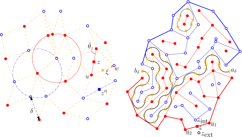
Figure 1. (Left) Local view of an isoradial grid. Primal vertices $u$ in solid red; dual vertices $w$ in hollow blue; rhombus edges $\xi$ in dashed orange. Also note the primal edge $z$ and dual edge $z^{\prime\dagger}$, both diagonals of their respective rhombi (also denoted $z,z^{\prime}$). (Right) A sample FK-Ising configuration. Primal edges $E$ in solid red; dual edges $E^{*}$ in solid blue; the interface $\gamma$ in solid black; boundary primal/dual wiring in bold. Local notation around a boundary primal edge $z$ shown in bottom.

Z-Invariant Weights and Mass Scaling

On isoradial graphs, we consider the family of local weights on the edges (i.e. rhombi) parametrised by the elliptic modulus $k\in\left[0,1\right]$: the Z-invariant weights, which coincides with the critical weights in [ChSm12] when $k=0$, which we call also the massless weights. While we study the model in the vicinity of $k=0$, let us note here that the case $k=1$ corresponds to the degenerate case where all edges must be sampled.

Locally, the weights are conveniently written in terms of abstract angles $\hat{\theta}_{z}\in\left[\bar{\theta}_{z},\frac{\pi}{2}\right]$ assigned to each edge $z$ satisfying the following relation $k$ and the geometric rhombus half-angle $\overline{\theta}_{z}$:

$$u\left(\hat{\theta}_{z}|k\right)=\frac{u\left(\pi/2|k\right)}{\pi/2}\cdot\overline{\theta}_{z}=:\frac{K(k)}{\pi/2}\overline{\theta}_{z},$$

where $u\left(\varphi|k\right):=\int_{0}^{\varphi}\frac{d\theta}{\sqrt{1-k^{2}\sin^{2}\theta}}$, and the elliptic quarter-period $K(k):=F\left(\pi/2|k\right)$. Under this correspondence, we have the convenient relations (which may be taken as the definitions for the functions on the left hand side):

$$\operatorname{sn}\left(\frac{K(k)}{\pi/2}\overline{\theta}_{z}\right)=\sin\hat{\theta}_{z},\operatorname{cn}\left(\frac{K(k)}{\pi/2}\overline{\theta}_{z}\right)=\cos\hat{\theta}_{z},\operatorname{sc}\left(\frac{K(k)}{\pi/2}\overline{\theta}_{z}\right)=\tan\hat{\theta}_{z}.$$

To take the scaling limit to obtain the massive regime, we need to scale $k^{2}\sim 8m\delta$ in the limit $\delta\downarrow 0$ for some fixed $m>0$. Equivalently, we take the real nome $q:=\exp\left[-\pi K(\sqrt{1-k^{2}})/K(k)\right]$ and scale $q\sim\frac{1}{2}m\delta$ (since $K$ is increasing, $q$ is also increasing in $k$, and $q\sim k^{2}/16$ for small $k$; see [DLMF, 19.5.5]). Unfortunately, the standard notation $m$ for the mass parameter is also used for the square of $k$ in the elliptic function literature; however, we choose to exclusively use $m$ for the former meaning, assuming some relation $q=q(\delta)$ such that (say) $q\leq m\delta$ and $\delta^{-1}q\xrightarrow{\delta\downarrow 0}\frac{m}{2}$ to have been fixed whenever talking about a ($m$-)massive scaling limit.

The parameters $\hat{\theta}_{z}$, and thus the relative weight of open edges, increase in $k,q$ (see, e.g. [CaTo83]). In fact, as $\delta\downarrow 0$, we have

(1.1) $$\hat{\theta}_{z}=\overline{\theta}_{z}+m\delta\sin 2\bar{\theta}_{z}+O(\delta^{2}),$$

as seen from $\tan\hat{\theta}_{z}=\left(1+4q\right)\tan\overline{\theta}_{z}+O(q^{2})$ [DLMF, 20.2(i), 22.2.9].

FK-Ising Model

Consider a (primal) configuration, a subset $E\subset\lozenge\left(\Omega^{\delta}\right)$ of primal edges, and its dual configuration $E^{*}$, consisting of dual edges corresponding to the primal edges in $\lozenge\left(\Omega^{\delta}\right)\setminus E$ (Figure 1R). To implement the boundary condition, we consider the boundary edges on each wired arc as part of $E$ and each free arc as $E^{*}$. We primarily consider 2-point and 4-point (generalised) Dobrushin boundary conditions: they are respectively defined on marked domains $\left(\Omega^{\delta},a^{\delta},b^{\delta}\right)$ and $\left(\Omega^{\delta},a^{\delta},b^{\delta},c^{\delta},d^{\delta}\right)$, with the boundary condition alternating between free and wired, starting from the free arc $\left(a_{w}^{\delta}b_{w}^{\delta}\right)$. We will announce explicitly the setup of the model whenever writing $\mathbb{P}$.

An edge $z\in E$ is termed open (accordingly, $z\in E^{*}$ closed or dual-open). Given the connections made by $E$, a connected component of $\Gamma\left(\Omega^{\delta}\right)$ is called an open or primal cluster (accordingly, closed or dual cluster for $E^{*}$ and $\Gamma^{*}\left(\Omega^{\delta}\right)$). Then given any corner $\left\langle uw\right\rangle\in\Upsilon\left(\Omega^{\delta}\right)$, there is a curve (unique up to homotopy away from $E,E^{*}$) separating the open cluster of $u$ and the closed cluster of $w$. Any such curve might exit the domain through one of the marked boundary corners, in which case it is an interface curve (see Figure 1R and also Section 2.1) between boundary clusters, or be simple loops within the domain, whose number we denote as $\#\text{loops}\left(E\right)$. Define the ($q$-)massive FK-Ising model on $\Omega^{\delta}$ as the probability measure $\mathbb{P}$ on subsets of $\lozenge\left(\Omega^{\delta}\right)$ given by:

$$\mathbb{P}\left(E\right)\propto\sqrt{2}^{\#\text{loops}\left(E\right)}\prod_{z\in E}\sin\frac{\hat{\theta}_{z}}{2}\prod_{z\in\lozenge\setminus E}\sin\left(\frac{\pi}{4}-\frac{\hat{\theta}_{z}}{2}\right).$$

Clearly, the dual configuration $E^{*}$ has the FK-Ising law sampled from the dual graph with weights switched and free arcs being dual-wired. In fact, while we only consider on the primal graph the subcritical massive scaling limit (where $\hat{\theta}_{z}>\bar{\theta}_{z}$) the dual configuration has a supercritical law, and thus our treatment covers both the sub- and supercritical massive regimes simultaneously.

Let us finish by recalling the basic notions and properties of the model, for which [Gri06] serves as a comprehensive reference. We are primarily interested in crossing events, where given subsets of the plane are connected by an open cluster in $E$. It is clear that conditioning on a bounded number of edges only affect the probability measure by a bounded factor, a consequence of the finite energy property of the model: therefore, the probabilities for crossing of sets which are bounded lattice spacings apart are uniformly comparable. This in particular allows for speaking of the ’same’ domain endowed with different boundary conditions, which might require in reality adding or taking way some layers of (dual-)wired edges, which only affect crossing events up to a uniform factor.

(Open) crossings are the archetypal examples of increasing events: if the event contains $E$, then any superset of $E$ is also in the event. The classical Fortuin-Kasteleyn-Ginibre (FKG) inequality says that increasing events are positively correlated, that is, conditioning on an increasing event only augments another increasing event’s probability. Note also that the probability of an increasing event increases when the weight parameter $\hat{\theta}_{z}$ increases or the boundary condition along some segment switches from free to wired.

1.2. Statement of the Theorems

Our fundamental result is on convergence of discrete fermionic observables, to be defined precisely in Section 2. These are discrete massive holomorphic functions, which converge to continuous functions with analogous properties: we call a function (see Section 3.1 for notes on regularity) $f$ defined on a simply connected $\Omega\subset\mathbb{C}$ massive holomorphic if it satisfies the Bers-Vekua equation

$$\bar{\partial}f+mi\bar{f}=0\text{ in }\Omega,$$

with constant coefficient $m>0$. Here we use the standard Wirtinger derivatives $\partial:=\frac{1}{2}\left(\partial_{x}-i\partial_{y}\right)$ and $\bar{\partial}:=\frac{1}{2}\left(\partial_{x}+i\partial_{y}\right)$.

First, we show convergence of the 2-point observable, also known as the fermionic martingale observable (see [MaSm10]). We say that a family $\left\{F^{\delta}\right\}_{\delta>0}$ of discrete function defined on $\lozenge\left(\Omega_{\delta}\right)$ converges to $f$ if $f^{\delta}:=\left.f\right|_{\lozenge\left(\Omega_{\delta}\right)}$ is (locally uniformly) close to $F^{\delta}$ as $\delta\downarrow 0$.

Theorem 1.1.

On a marked simply connected domain $\left(\Omega,a,b\right)$, the 2-point discrete massive fermionic observable $F_{\left(\Omega^{\delta},a^{\delta},b^{\delta}\right)}^{\delta}$ (Definition 2.1 and Proposition 2.2) converges as $\delta\downarrow 0$ uniformly on compact subsets to the massive holomorphic limit $f_{\left(\Omega,a,b\right)}$ as in Definition 5.2.

Proof.

One may extract from any subset of $\left\{F_{\left(\Omega^{\delta},a^{\delta},b^{\delta}\right)}^{\delta}\right\}_{\delta>0}$ a subsequence which converges to a smooth function on $\Omega$ uniformly in compact subsets by Proposition 2.7 and Remark 4.7. Then it remains to show that the limit is the unique function satisfying the conditions laid out in Definition 5.2, which is shown in Proposition 5.8. ∎

Now we move to convergence of the crossing probability on a conformal quadrilateral with 4-point Dobrushin boundary condition, which in turn comes from convergence of the 4-point observable (Definition 2.4). Given the conformal quadrilateral $\left(\Omega^{\delta},a^{\delta},b^{\delta},c^{\delta},d^{\delta}\right)$, we denote by $\stackrel{{\scriptstyle\leftrightarrow}}{{\Omega^{\delta}}}$ the event that the conformal quadrilateral is horizontally (open) crossed, which we will fix as the event that the two boundary clusters respectively containing $\left(b_{\text{b}}^{\delta}c_{\text{b}}^{\delta}\right)$ and $\left(d_{\text{b}}^{\delta}a_{\text{b}}^{\delta}\right)$ are connected by primal edges in $E$.

Theorem 1.2.

For any conformal quadrilateral $\left(\Omega,a,b,c,d\right)$, the crossing probability

$$\mathbb{P}\left[\stackrel{{\scriptstyle\leftrightarrow}}{{\Omega^{\delta}}}\right]=:\mathrm{P}^{\delta}$$

of the massive 4-point Dobrushin FK-Ising model on $\left(\Omega^{\delta},a^{\delta},b^{\delta},c^{\delta},d^{\delta}\right)$ converges to a limit $\mathrm{P}^{\delta}\xrightarrow{\delta\downarrow 0}\mathrm{p}_{m}\in\left(0,1\right)$.

$\mathrm{p}_{m}$ is uniquely determined by the condition that if $t_{m}:=\frac{\mathrm{p}_{m}}{1-\mathrm{p}_{m}}$, then $\varkappa_{m}:=\left[\frac{t_{m}^{2}+\sqrt{2}t_{m}}{t_{m}^{2}+\sqrt{2}t_{m}+1}\right]^{2}\in\left(0,1\right)$ is the unique value for which there exists a massive holomorphic function $f_{\left(\Omega,a,b,c,d\right)}$ in Definition 5.5.

Proof.

The fact that $\mathrm{P}^{\delta}$ is encoded in the discrete 4-point observable $F_{\left(\Omega^{\delta},a^{\delta},b^{\delta},c^{\delta},d^{\delta}\right)}^{\delta}$ of Definition 2.4 through the value $\varkappa^{\delta}$ defined in Proposition 2.8 is a combinatorial calculation identical to the critical case, see [ChSm12, (6.6)]. As in the 2-point case, we may extract subsequential limits from the set of discrete observable, which we show to be unique in Corollary 5.17. ∎

Application: RSW-Type Estimates and Upper Bound for the Characteristic Length

Using a degenerate case of the 2-point observable, we may show the following uniform estimate of the crossing probability of a rectangle of given aspect ratio, also known as a Russo-Seymour-Welsh (RSW) type estimate. [DGP14] shows the following on the square lattice. We give a proof on the isoradial graph, using the general method established in [DHN11]. Note that one may alternatively use the 4-point connection probability from Theorem 1.2 to obtain annulus crossing estimates rather straightforwardly, by using the argument of [Che20, Section 5.6].

Recall that we discretise a rectangle $R(\rho):=\left(0,1\right)+\left(0,\rho i\right)$ using the intersection with an isoradial lattice. The following is stated for the subcritical primal model, but it also implies the analogue for the supercritical regime by duality. Note that we may standardise rectangles of any size into $R(\rho)$ by rescaling the mass (which then gets multiplied by the original horizontal side length). Here horizontal crossing intuitively refers to a crossing event from left to right sides.

Theorem 1.3.

Let $m>0$. There is a constant $\operatorname{c}(\rho,\eta,m)>0$ such that

$$\operatorname{c}(\rho,\eta,m)\leq\mathbb{P}\left[\stackrel{{\scriptstyle\leftrightarrow}}{{R(\rho)^{\delta}}}\right]\leq 1-\operatorname{c}(\rho,\eta,m),$$

for the massive FK-Ising model with $q\leq m\delta$ and any boundary condition on the discrete rectangle $R(\rho)^{\delta}$.

Proof.

It suffices to show the upper bound for wired boundary condition; other boundary conditions and the lower bound follow easily from monotonocity in weights and duality. More specifically, we will show that the dual model has a vertical crossing with probability bounded away from zero. It also suffices to prove the estimate for some small fixed $m_{0}>0$, since we may use the estimate at $m_{0}$ multiple times to obtain crossing estimates of larger rectangles (using FKG inequality, cf. the Bernouilli case in e.g. [Nol08]) at $m_{0}$, which then translate to the above result for normalised rectangles at larger masses.

Consider the (discretised) bottom and top middle boundary segments $\left[\left(\frac{1}{3}\right)^{\delta},\left(\frac{2}{3}\right)^{\delta}\right]$ and $\left[\left(\frac{1}{3}+\rho i\right)^{\delta},\left(\frac{2}{3}+\rho i\right)^{\delta}\right]$. Then defining the number of disjoint dual vertical crossings as $N$, we have the second-moment estimate

$$1-\mathbb{P}\left[\stackrel{{\scriptstyle\leftrightarrow}}{{R(\rho)^{\delta}}}\right]\geq\mathbb{P}\left[N>0\right]\geq\frac{\mathbb{E}\left[N\right]^{2}}{\mathbb{E}\left[N^{2}\right]},$$

so we need to give a lower bound for the numerator and an upper bound for the denominator. By monotonicity, the latter, specifically

$$\mathbb{E}\left[N^{2}\right]\leq\operatorname{C}\left(\rho,\eta\right)\delta^{2},$$

may be obtained at criticality ($m=0$); this is the content of [DHN11, Proposition 4.3], which is technically stated only for the square lattice but their strategy applies with almost no modification on isoradial lattice with angle bound $\eta>0$. Namely, [DHN11, Lemma 3.3] connects the probability that the critical FK-interface passes through a boundary corner to harmonic measure estimates through the use of the fermionic observable (see Lemma 2.6 and the proof for isoradial analogues). These estimates are obtained by comparison and explicit estimates on standard domains, which are straightforward to obtain in the isoradial case using, e.g., [ChSm12, Lemma A.3]. For the sake of conciseness we do not replicate the full proof.

The ’massive content’ is in the lower bound for the numerator: we prove that $\mathbb{E}\left[N\right]\geq\operatorname{c}(\rho,\eta)\delta$ for some small $m_{0}>0$ in Corollary 4.13. This finishes the proof. ∎

[DGP14, Theorem 1.2] and [DuMa20, Theorem 1.3] respectively provide lower and upper bounds on the square lattice for the characteristic length (called correlation length in the former), defined as the size (in terms of lattice spacings) of the smallest rectangle which is crossed with at least a given cutoff probability (stated without loss of generality in terms of the subcritical primal model). Note that $q\propto p-p_{c}$ in their setup.

Corollary 1.4.

For $\rho>0$, consider the $q$-massive FK-Ising model with any given boundary condition on the discrete rectangle $R(\rho)^{\delta}$. For fixed $\epsilon\in\left(0,1\right)$, define the characteristic length

$$\left(L_{\rho,\epsilon,q}\right)^{-1}:=\sup\left\{\delta>0:\mathbb{P}\left[\stackrel{{\scriptstyle\leftrightarrow}}{{R(\rho)^{\delta}}}\right]\geq 1-\epsilon\right\}.$$

Then for all small $\epsilon>0$, there are constants $0<\operatorname{c}(\rho,\eta,\epsilon)<\operatorname{C}(\rho,\eta,\epsilon)$ such that

(1.2) $$\operatorname{c}(\rho,\eta,\epsilon)\leq qL_{\rho,\epsilon,q}\leq\operatorname{C}(\rho,\eta,\epsilon).$$

Proof.

The lower bound is essentially the crossing bound of Theorem 1.3: if there is no such constant, there is a sequence $q_{j}\delta_{j}^{-1}\to 0$ such that $\mathbb{P}\left[\stackrel{{\scriptstyle\leftrightarrow}}{{R(\rho)^{\delta}}}\right]$ remains at least $1-\epsilon$, so for any $\epsilon$ smaller than the upper bound in Theorem 1.3, we obtain a contradiction. The upper bound is shown in Section 6.2, starting from the 4-point Dobrushin boundary case (Corollary 6.4) given before the general proof. ∎

Other Implications

[DGP14] has highlighted a behaviour in the massive FK-Ising model which qualitatively differ from that of massive Bernouilli percolation on triangular lattice (e.g. [Nol08]): the characteristic length $L_{\rho,\epsilon,q}$ scales like $q^{-1}$, which suggests that it is not solely determined by the critical four-arm exponent as in the Bernouilli percolation case. That is, the characteristic length cannot be estimated by independently flipping the pivotal points, where macroscopic four-arms start. In the massive Bernouilli percolation, the analysis of four-arm exponents has led to uncovering the mutual singularity (i.e. absolutely continuous in neither direction) of the massive and the critical scaling limits, both in terms of the interface curve [NoWe09] and the quad-crossing probability [Aum13, GPS18]. The latter is done by considering asymptotically smaller quads, where the model breaks up into independent pieces and crossing probabilities are perturbed by a quantity determined by the four-arm exponent. In our case, restrictions to these small quads do not become independent, and crossing probabilities depend on the boundary condition; nonetheless, hoping to carry out similar analysis in future works, we show in the case of the 4-point Dobrushin boundary condition that the perturbation to the quad-crossing probability decays as $m\downarrow 0$ (corresponding to reducing quad size at a fixed mass) like $m$ (Corollary 6.2).

With respect to the interface, we happen to prove massive versions of the two results which implied convergence of the critical FK-Ising interface in law ([CDHKS14], see also [MaSm10]): convergence of the discrete martingale observable to a unique limit (Theorem 1.1) and the RSW-type crossing estimate (Theorem 1.3; [DGP14, Theorem 1.3] on the square lattice). The latter in fact implies that some Hölder exponent of the massive FK-Ising interface is bounded [KeSm17]. The reason that we cannot then easily conclude that there is a unique limit of the law of the discrete interface is because the analysis of the continuous martingale observable turns out to be significantly more convoluted than in the critical case; this is to be expected, given that the massive scaling limit of the interface may well have a distribution which is mutually singular with the critical limit $SLE(16/3)$ (as in the case of the massive percolation interface and $SLE(6)$, massive uniform spanning tree and $SLE(8)$ [MaSm10], and conjectured in, e.g., [GPS18] for any $SLE(\kappa)$ with $\kappa\in(4,8]$).

1.3. Structure of the Paper

This paper is organised as follows. In Section 2, we relate the probabilistic model to discrete complex analysis by introducing discrete fermionic observables for the 2- and 4-point boundary conditions; they satisfy massive s-holomorphicity, a consequence of which is shown to be the existence of the discrete square integral as mentioned above. We finish by translating boundary conditions for the model to the Riemann-Hilbert boundary value problem for the s-holomorphic observable and its square integral. In Section 3, we define massive holomorphic functions, which are continuous counterparts of the massive s-holomorphic functions and is shown later to be their scaling limits. We also consider their conformal pullbacks to smooth domains $D$, which satisfy a non-constant version of massive holomorphicity. Like their discrete ancestors, they have well-defined (imaginary parts of) square integrals, which are then analysed as solutions of an elliptic PDE. Near the boundary, we analyse both massive holomorphic functions and their pullbacks under the umbrella of generalised analytic functions, while deferring some of the computations to the Appendix. In Section 4, we pursue a discrete version of the regularity theory in the previous section. The discrete square integral is seen to be critical in the analysis, and many properties of the continuum integral, such as the maximum principle, have analogues here. These results imply a certain bulk precompactness for the collection of discrete observables. We then show that the discrete boundary condition is preserved in the limit and provide required estimates of the degenerate observable used in the proof of the RSW-type estimate, both of which can be done without fixing a unique continuum limit. In Section 5, we show that any subsequential limit of the discrete observables has to be unique, therefore finishing the proof of their convergence. In the 2-point case, we use primarily potential-theoretic estimates of the Dirichlet Laplacian Green function; in the 4-point case, we use maximum principle to show that the 4-point square integral naturally breaks up into two 2-point ones. In Section 6, we study how the primal crossing probability in the 4-point boundary condition, which is exactly encoded in the continuum square integral, varies as $m$ tends to $0$ and $\infty$. We also show how to use the latter and RSW-type estimates to get the desired asymptotic for the characteristic length $L$. We finish by providing more involved computations and theory reference in the Appendix.

Acknowledgement

The author is supported by a KIAS Individual Grant (MG077201, MG077202) at Korea Institute for Advanced Study. The author thanks Dmitry Chelkak for inviting him to École Normale Superieure Paris and in particular informing him of [Che20, Lemma A.2], inspiring the proof of Proposition 5.8. The author also thanks Clément Hongler, Konstantin Izyurov, Kalle Kytölä, Rémy Mahfouf, Francesco Spadaro, and Yijun Wan for interesting discussions.

2. Massive S-Holomorphic Observables

2.1. Fermionic Observables

In this section, we define the main discrete object of our study, the 2- and 4-point fermionic observables. These are discrete functions built to reflect the combinatorics of the discrete (FK-)Ising model which then have nontrivial scaling limits which we can identify in the continuum. The following definition is essentially same as that in [ChSm12, (2.2)], albeit the expectation is evaluated with different weights (if $q\neq 0$).

Consider the 2-point case first. Recall a corner $\xi$ is associated with the direction $\nu_{\xi}$, the unit complex number pointing from the primal vertex to the dual vertex. Given any configuration, we may draw the interface $\gamma^{\delta}$ as the (unique up to homotopy) curve separating the open cluster of $b_{\text{b}}^{\delta}$ from the dual cluster of $b_{\text{w}}^{\delta}$. We will start $\gamma^{\delta}$ from $b^{\delta}$ (i.e. the midpoint of $b_{\text{b}}^{\delta}$ and $b_{\text{w}}^{\delta}$) and go through each corner (or the midpoint thereof) orthogonally: see Figure 1R.

Definition 2.1.

On every corner $\xi$ of $\left(\Omega^{\delta},a^{\delta},b^{\delta}\right)$, define the $2$-point discrete fermionic observable $F_{\left(\Omega^{\delta},a^{\delta},b^{\delta}\right)}^{\delta}$ by the FK-Ising expectation

(2.1) $$F_{\left(\Omega^{\delta},a^{\delta},b^{\delta}\right)}^{\delta}\left(\xi\right)=\left(\frac{1}{2\delta\nu_{b^{\delta}}}\right)^{1/2}\mathbb{E}\left[\mathbf{1}\left(\xi\in\gamma^{\delta}\right)\cdot e^{-\frac{i}{2}\operatorname{w}(\gamma^{\delta}:b^{\delta}\rightsquigarrow\xi)}\right],$$

defined up to a global sign (corresponding to the choice of the square root), where $\operatorname{w}(\gamma^{\delta}:b^{\delta}\rightsquigarrow\xi)$ is the total turning of the tangent of $\gamma^{\delta}$ starting from $b^{\delta}$ to $\xi$.

The sign of $F_{\left(\Omega^{\delta},a^{\delta},b^{\delta}\right)}^{\delta}$, if required, may be easily fixed in any given domain $\Omega$, say, by requiring a strictly positive real part in a small fixed neighbourhood; we did not specify such a choice above for the sake of conciseness and naturalness. See also (the proof) of [ChSm12, Theorem 4.3].

Since $\operatorname{w}$ is determined by $\xi$ up to integer multiples of $2\pi$ (recall $\gamma^{\delta}$ passes through $\xi$ orthogonally with primal vertex on the right), $F_{\left(\Omega^{\delta},a^{\delta},b^{\delta}\right)}^{\delta}\left(\xi\right)$ necessarily lies on the line $\left(i\nu_{\xi}\right)^{-1/2}\mathbb{R}$. Therefore, they are not considered full complex values of the functions: instead, they are projections (on the complex plane) on respective lines of the full values to be defined on edges. We extend their definitions to edges (rhombus centres) through the following proposition. To account for the difference between the abstract angle $\hat{\theta}_{z}$ and the geometric angle $\overline{\theta}_{z}$, we consider $\hat{\xi}$ (depending implicitly on $z$) to be the rhombus edge corresponding to $\xi$ in the virtual rhombus where $\overline{\theta}_{z}$ is replaced by $\hat{\theta}_{z}$: i.e. define $\nu_{\hat{\xi}}:=e^{\pm i\left(\hat{\theta}_{z}-\overline{\theta}_{z}\right)}\nu_{\xi}$ with sign alternating along the rhombus. The idea of the below notion and proof precisely comes from rotating (in terms of the fixed-phase corner values) the critical s-holomorphicity relation [ChSm12, (2.6)] between the values at $z$ and the virtual corner $\hat{\xi}$ to the physical rhombus with angle $\hat{\theta}_{z}$.

Proposition 2.2.

At every interior edge (rhombus centre) $z\in\lozenge$, there may be assigned a unique value $F^{\delta}(z)=F_{\left(\Omega^{\delta},a^{\delta},b^{\delta}\right)}^{\delta}(z)$ which makes the following equality true:

(2.2) $$\text{Proj}\left[F^{\delta}(z);\left(i\nu_{\hat{\xi}}\right)^{-1/2}\mathbb{R}\right]=\left(\frac{\nu_{\hat{\xi}}}{\nu_{\xi}}\right)^{-1/2}F^{\delta}(\xi),$$

where $\xi$ is any of the four edges of the rhombus (i.e. corners) centred at $z$ and $\left(\frac{\nu_{\hat{\xi}}}{\nu_{\xi}}\right)^{1/2}$ should be chosen with positive real part.

Proof.

This is a rephrasing in the Z-invariant case of the so-called 3-point propagation equation, which is purely combinatorial and valid with any local weight (parametrised by abstract angle $\hat{\theta}$ as in introduction). Around a rhombus centre $z$, consider the double-valued real observable $X$ branching at $z$:

$$X(\xi)=\left(i\nu_{\xi}\right)^{1/2}F^{\delta}(\xi).$$

Then for any triple of adjacent corners $\xi_{0,1,2}$ (going counterclockwise) around $z$, the propagation equation reads (see e.g. [Che20, (1.5)])

$$X\left(\xi_{1}\right)=\cos\hat{\theta}_{z}\cdot X\left(\xi_{2}\right)+\sin\hat{\theta}_{z}\cdot X\left(\xi_{0}\right).$$

By [ChSm12, Lemma 3.4], this implies the existence of a unique value $F^{\delta}(z)$ that satisfies the following relation for each $\xi$,

$$\text{Proj}\left[F^{\delta}(z);\left(i\nu_{\hat{\xi}}\right)^{-1/2}\mathbb{R}\right]=\left(i\nu_{\hat{\xi}}\right)^{-1/2}X(\xi),$$

which is equivalent to (2.2), being careful to use a single branch $\left(i\nu\right)^{1/2}$ such that $\left(i\nu_{\xi}\right)^{1/2}$ is always perturbed by $e^{\pm\frac{i}{2}\left(\hat{\theta}_{z}-\overline{\theta}_{z}\right)}$ when $\nu_{\xi}$ is perturbed by $e^{\pm i\left(\hat{\theta}_{z}-\overline{\theta}_{z}\right)}$ (note $\hat{\theta}-\overline{\theta}\in\left[0,\frac{\pi}{2}\right)$). ∎

By Lemma A.2, (2.2) is a discrete notion of massive holomorphicity $\bar{\partial}f+im\bar{f}=0$. Equivalent massive observables have been considered on the square lattice [BeDu12, DGP14, HKZ15].

Definition 2.3.

We call (2.2) (($q,k$)-massive) s-holomorphicity.

In the case of $4$-point observables, we need to work with two interface curves: to define an observable as in Definition 2.1, we need to merge them into a single interface. A natural way of doing this, developed in the proof of [ChSm12, Theorem 6.1], is to externally connect the boundary segments. We summarise the construction here.

Compared to the original measure with two interface curves, externally dual-connecting the two dual-wired boundary segments (specifically, draw an external dual edge $\left\langle a_{\text{w}}^{\delta}d_{\text{w}}^{\delta}\right\rangle$ closely to the original wired segment $\left(d^{\delta}a^{\delta}\right)$) yields a measure $\mathbb{P}_{\text{p}}$ which augments the relative weights of configurations not in $\stackrel{{\scriptstyle\leftrightarrow}}{{\Omega^{\delta}}}$ by a factor of $\sqrt{2}$. On the other hand, connecting the two primal segments (draw an external primal edge $\left\langle c_{\text{b}}^{\delta}d_{\text{b}}^{\delta}\right\rangle$ close to the dual-wired segment $\left(c^{\delta}d^{\delta}\right)$) externally augments the relative weights of configurations in $\stackrel{{\scriptstyle\leftrightarrow}}{{\Omega^{\delta}}}$ by a factor of $\sqrt{2}$. In both cases, we define massive s-holomorphic observables $F_{\text{p}}^{\delta},F_{\text{d}}^{\delta}$ by using (2.1), drawing single interfaces through $b^{\delta}$ thanks to addition of the external edges as above. Recall the probability $\mathrm{P}^{\delta}=\mathbb{P}\left[\stackrel{{\scriptstyle\leftrightarrow}}{{\Omega^{\delta}}}\right]=\mathbb{P}_{\text{p}}\left[\stackrel{{\scriptstyle\leftrightarrow}}{{\Omega^{\delta}}}\right]$ that the primal segments $\left(b^{\delta}c^{\delta}\right)$ and $\left(d^{\delta}a^{\delta}\right)$ are (internally) connected.

Definition 2.4.

Let $\mathrm{Q}^{\delta}:=1-\mathrm{P}^{\delta}$. Define the $4$-point Dobrushin fermionic observable $F_{\left(\Omega^{\delta},a^{\delta},b^{\delta},c^{\delta},d^{\delta}\right)}^{\delta}$ by

$$F_{\left(\Omega^{\delta},a^{\delta},b^{\delta},c^{\delta},d^{\delta}\right)}^{\delta}:=\frac{\mathrm{P}^{\delta}\left(\sqrt{2}\mathrm{P}^{\delta}+\mathrm{Q}^{\delta}\right)F_{\text{d}}^{\delta}+\mathrm{Q}^{\delta}\left(\mathrm{P}^{\delta}+\sqrt{2}\mathrm{Q}^{\delta}\right)F_{\text{p}}^{\delta}}{\mathrm{P}^{\delta}\left(\sqrt{2}\mathrm{P}^{\delta}+\mathrm{Q}^{\delta}\right)+\mathrm{Q}^{\delta}\left(\mathrm{P}^{\delta}+\sqrt{2}\mathrm{Q}^{\delta}\right)},$$

on the corners of $\Omega^{\delta}$ and then edges by (2.2).

This observable encodes the desired connection probability $\mathrm{P}^{\delta}$ through the boundary value problem of Proposition 2.8.

2.2. Integral of the Square and the Boundary Value Problem

In this section, we define square integrals of massive s-holomorphic functions (functions $F$ on rhombus centres and edges satisfying (2.2)). These are discrete counterparts of the imaginary part of the line integral $\int F^{2}dz$.

Lemma 2.5.

Given a massive s-holomorphic function $F$ on a simply connected discrete domain $\Omega_{\delta}$ , the real-valued function $H$ on $\Lambda$ constructed by:

(2.3) $$H(u)-H(w):=2\delta\cdot\left|F(\xi)\right|^{2},$$

for a corner $\xi=\left\langle uw\right\rangle$ with adjacent $u\in\Gamma,w\in\Gamma^{*}$, is well defined.

We will write $H:=\text{Im}\int^{\delta}F^{2}dz$ in the sense that, the discrete derivatives across the centre $z\in\lozenge$ of the rhombus bordered by $u,w,u_{z},w_{z}$ (see Figure 5L) satisfy

(2.4) $$H(u_{z})-H(u) =\frac{\cos\hat{\theta}_{z}}{\cos\bar{\theta}_{z}}\text{Im}\left[\left(u_{z}-u\right)\cdot F(z)^{2}\right],$$

$$H(w_{z})-H(w) =\frac{\sin\hat{\theta}_{z}}{\sin\bar{\theta}_{z}}\text{Im}\left[\left(w_{z}-w\right)\cdot F(z)^{2}\right].$$

Proof.

It suffices to check the well-definedness on each rhombus, i.e. going around the $4$ corners. Then

$$\left|F(z)\right|^{2}=\left|F(\left\langle uw\right\rangle)\right|^{2}+\left|F(\left\langle u_{z}w_{z}\right\rangle)\right|^{2}=\left|F(\left\langle uw_{z}\right\rangle)\right|^{2}+\left|F(\left\langle u_{z}w\right\rangle)\right|^{2},$$

immediate from (2.2), in fact implies well-definedness. Both statements in fact can be interpreted as reformulation of the massless case [ChSm12, Proposition 3.6] since $F$ may be considered a massless s-holomorphic function on the virtual rhombus with half-angle replaced $\bar{\theta}\to\hat{\theta}$ and rotated values on corners as in Proposition 2.2. ∎

Now we present the so-called discrete Riemann-Hilbert boundary value problem which the observables satisfy, which are discrete ancestors of the continuous boundary value problems of Definition 3.10. While it is most intuitively phrased in terms of boundary phases of the massive s-holomorphic observable $F$, the version that translates most naturally to possibly rough domains is the corresponding condition for $H$. Unlike their continuous counterparts (Proposition 3.11 and Definition (3.10)), these two discrete conditions are equivalent.

The following boundary condition, essentially identical to that in the critical case ([ChSm12, (2.5)] and the boundary modification combining elements of [ChSm12, DHN11, CHI15]), is satisfied both for the $2$- and $4$-point observables on their respective free and wired arcs, so we write $F^{\delta}$ for either. The definition of $F^{\delta}$ and extension by (2.2) holds for all edges in $\lozenge\left(\Omega^{\delta}\right)$; this gives enough information to define $H^{\delta}:=\operatorname{Im}\int^{\delta}\left(F^{\delta}\right)^{2}dz$ on all (primal and dual) vertices on the closed domain bounded by the boundary arcs $\partial\lozenge\left(\Omega^{\delta}\right)$ (i.e. where the boundary conditions are set) and the marked boundary corners. We now extend $F^{\delta}$ to $\partial\lozenge\left(\Omega^{\delta}\right)$, which then yields a natural extension of $H^{\delta}$ to the external vertices, i.e. the vertices on the outer halves of boundary rhombi bisected by $\partial\lozenge\left(\Omega^{\delta}\right)$.

Lemma 2.6.

A 2- or 4-point observable $F^{\delta}$ may be extended to the boundary edges $\underline{z}\in\partial\lozenge\left(\Omega^{\delta}\right)$ satisfying the following equivalent discrete Riemann-Hilbert boundary conditions.

Suppose $\underline{z}$ is on the wired arc (set $\upsilon:=1$) such that the corresponding rhombus $\left\langle\underline{u}_{1}\underline{z}_{\text{int}}\underline{u}_{2}\underline{z}_{\text{ext}}\right\rangle$ (see Figure 1R) is bisected by the primal boundary edge $\left\langle\underline{u}_{1}\underline{u}_{2}\right\rangle$ with the dual vertex $\underline{w}_{\text{int}}$ in the interior. Consider the unit tangent vector $\nu_{\text{tan}}=\nu_{\text{tan}}(\underline{z})=\frac{\underline{u}_{2}-\underline{u}_{1}}{\left|\underline{u}_{2}-\underline{u}_{1}\right|}$.

• $\left(RH\right)_{F}$: $F^{\delta}\left(\underline{z}\right)$ may be defined as the unique value satisfying (2.2) (with its two interior corners), which belongs to $\sqrt{\frac{\upsilon}{\nu_{\text{tan}}}}\mathbb{R}$.

• $(RH)_{H}$: the square integral $H^{\delta}:=\operatorname{Im}\int^{\delta}\left(F^{\delta}\right)^{2}dz$ may be defined at $\underline{z}_{\text{ext}}$ such that it

  • stays constant on $\underline{u}_{1},\underline{u}_{2},\underline{z}_{\text{ext}}$;

  • is consistent with $F^{\delta}\left(\underline{z}\right)$ and (2.4), as long as one replaces $\sin\hat{\theta}_{\underline{z}}\to\frac{\sin\hat{\theta}_{\underline{z}}+1}{2}$.

Note that (2.4) implies that $H^{\delta}(\underline{z}_{\text{int}})\leq H^{\delta}(\underline{z}_{\text{ext}})$: $H^{\delta}$ has nonnegative outer normal derivative on wired arcs.

On the free arc, we exchange the roles of primal and dual vertices, set $\upsilon:=-1$, and $\cos\hat{\theta}_{\underline{z}}\to\frac{\cos\hat{\theta}_{\underline{z}}+1}{2}$ on the boundary, yielding nonpositive outer normal derivative.

Proof.

Without loss of generality, we will check the wired arc case. Note that the interface $\gamma^{\delta}$ passes through $\left\langle\underline{u}_{1}\underline{z}_{\text{int}}\right\rangle$ if and only if it passes through $\left\langle\underline{u}_{2}\underline{z}_{\text{int}}\right\rangle$, and with deterministic $\operatorname{w}$ for both points. That is, we have

(2.5) $$F^{\delta}\left(\left\langle\underline{u}_{1,2}\underline{z}_{\text{int}}\right\rangle\right)=\frac{e^{-\frac{i}{2}\operatorname{w}(\gamma^{\delta}:b^{\delta}\rightsquigarrow\left\langle\underline{u}_{1,2}\underline{z}_{\text{int}}\right\rangle)}}{\left(2\delta\right)^{1/2}}\mathbb{P}\left[\left\langle\underline{u}_{1,2}\underline{z}_{\text{int}}\right\rangle\in\gamma^{\delta}\right],$$

with the probability coinciding both cases. Note that $\operatorname{w}(\gamma^{\delta}:b^{\delta}\rightsquigarrow\left\langle\underline{u}_{1}\underline{z}_{\text{int}}\right\rangle)-\left(\frac{\pi}{2}-\hat{\theta}_{\underline{z}}\right)=\operatorname{w}(\gamma^{\delta}:b^{\delta}\rightsquigarrow\left\langle\underline{u}_{2}\underline{z}_{\text{int}}\right\rangle)+\left(\frac{\pi}{2}-\hat{\theta}_{\underline{z}}\right)$, and in fact $e^{\frac{i}{2}\left[\operatorname{w}(\gamma^{\delta}:b^{\delta}\rightsquigarrow\left\langle\underline{u}_{1}\underline{z}_{\text{int}}\right\rangle)-\left(\frac{\pi}{2}-\hat{\theta}_{\underline{z}}\right)\right]}$ is a square root of $i\tau$. Then with this choice of the square root, it is simple to check that $F^{\delta}(\underline{z}):=\frac{\mathbb{P}\left[\left\langle\underline{u}_{1,2}\underline{z}_{\text{int}}\right\rangle\in\gamma^{\delta}\right]}{\sqrt{i\tau}\left(2\delta\right)^{1/2}\cos\left(\frac{\pi}{4}-\frac{\hat{\theta}_{\underline{z}}}{2}\right)}$ satisfies $(RH)_{F}$. The fact that $H(\underline{u}_{1})=H(\underline{u}_{2})$ is also clear from $\left|F^{\delta}\left(\left\langle\underline{u}_{1}\underline{z}_{\text{int}}\right\rangle\right)\right|=\left|F^{\delta}\left(\left\langle\underline{u}_{2}\underline{z}_{\text{int}}\right\rangle\right)\right|$ and (2.4).

On the other hand, if we define $H^{\delta}(\underline{z}_{\text{ext}})=H^{\delta}(\underline{u}_{1,2})$, then according to (2.4), it must be that $F^{\delta}(\underline{z})=\frac{\mathbb{P}\left[\left\langle\underline{u}_{1,2}\underline{z}_{\text{int}}\right\rangle\in\gamma^{\delta}\right]}{\sqrt{i\tau}\left(2\delta\right)^{1/2}\sin^{1/2}\hat{\theta}_{\underline{z}}}$. This discrepancy can be fixed by, as in the statement, replacing $\sin\hat{\theta}_{\underline{z}}\to\frac{\sin\hat{\theta}_{\underline{z}}+1}{2}$ which equals $\cos^{2}\left(\frac{\pi}{4}-\frac{\hat{\theta}_{\underline{z}}}{2}\right)$. ∎

Now we specialise and illustrate what the resulting boundary values of the square integrals of the discrete $2$- and $4$-point observables look like. Note that the previous lemma implies that it is possible to define a constant boundary value on an entire wired or free arc: on (say) a wired arc, the value $H(\underline{z}_{\text{ext}})=H(\underline{u}_{1,2})$ stays constant over each boundary edge $\underline{z}$, since two adjacent boundary edges share a vertex. It remains to specify the value on each boundary arc, which we now recall.

Proposition 2.7 ([ChSm12, (4.3)]).

One may fix the additive constant so that the square integral $H_{\left(\Omega^{\delta},a^{\delta},b^{\delta}\right)}^{\delta}:=\int^{\delta}\left(F_{\left(\Omega^{\delta},a^{\delta},b^{\delta}\right)}^{\delta}\right)^{2}dz$ of the $2$-point observable has the following boundary values:

$$H_{\left(\Omega^{\delta},a^{\delta},b^{\delta}\right)}^{\delta}\equiv 0\text{ on }\left(a^{\delta}b^{\delta}\right)\text{, }H_{\left(\Omega^{\delta},a^{\delta},b^{\delta}\right)}^{\delta}\equiv 1\text{ on }\left(b^{\delta}a^{\delta}\right).$$

Proof.

By Lemma 2.6, it suffices to characterise the difference of values at $b_{\text{w}}^{\delta}$ (which belongs to $\left(a^{\delta}b^{\delta}\right)$) and $b_{\text{b}}^{\delta}$ (which belongs to $\left(b^{\delta}a^{\delta}\right)$). But since any interface $\gamma^{\delta}$ passes through $b^{\delta}$, we have $F_{\left(\Omega^{\delta},a^{\delta},b^{\delta}\right)}^{\delta}(b^{\delta})=\frac{1}{\left(2\delta\right)^{1/2}}$. By (2.4), we have $H_{\left(\Omega^{\delta},a^{\delta},b^{\delta}\right)}^{\delta}(b_{\text{b}}^{\delta})-H_{\left(\Omega^{\delta},a^{\delta},b^{\delta}\right)}^{\delta}(b_{\text{w}}^{\delta})=1$, as desired. ∎

Proposition 2.8 ([ChSm12, (6.5)]).

One may fix the additive constant so that the square integral $H_{\left(\Omega^{\delta},a^{\delta},b^{\delta},c^{\delta},d^{\delta}\right)}^{\delta}:=\int^{\delta}\left(F_{\left(\Omega^{\delta},a^{\delta},b^{\delta},c^{\delta},d^{\delta}\right)}^{\delta}\right)^{2}dz$ of the $4$-point observable has the following boundary values:

$$H_{\left(\Omega^{\delta},a^{\delta},b^{\delta}\right)}^{\delta} \equiv 0\text{ on }\left(a^{\delta}b^{\delta}\right)\text{, }H_{\left(\Omega^{\delta},a^{\delta},b^{\delta}\right)}^{\delta}\equiv 1\text{ on }\left(b^{\delta}c^{\delta}\right)\text{, }$$

$$H_{\left(\Omega^{\delta},a^{\delta},b^{\delta}\right)}^{\delta} \equiv\varkappa^{\delta}\text{ on }\left(c^{\delta}d^{\delta}\right)\cup\left(d^{\delta}a^{\delta}\right),$$

where $T^{\delta}:=\frac{\mathrm{P}^{\delta}}{\mathrm{Q}^{\delta}},\varkappa^{\delta}:=\left[\frac{\left(T^{\delta}\right)^{2}+\sqrt{2}T^{\delta}}{\left(T^{\delta}\right)^{2}+\sqrt{2}T^{\delta}+1}\right]^{2}\in\left(0,1\right)$.

Proof.

Here, we need to study the jumps from $b_{\text{w}}^{\delta}$ to $b_{\text{b}}^{\delta}$, $d_{\text{w}}^{\delta}$ to $d_{\text{b}}^{\delta}$, and $a_{\text{b}}^{\delta}$ to $a_{\text{w}}^{\delta}$. We will give the final case as an illustration. Note that with the external dual edge $\left\langle a_{\text{w}}^{\delta}d_{\text{w}}^{\delta}\right\rangle$ as in $\mathbb{P}_{\text{p}}$, the interface $\gamma^{\delta}$ always goes through $a^{\delta}$ if and only if $\left(b^{\delta}c^{\delta}\right)$ and $(d^{\delta}a^{\delta})$ are internally dual-connected (with probability $\frac{\mathrm{P}^{\delta}}{\mathrm{P}^{\delta}+\sqrt{2}\mathrm{Q}^{\delta}}$), while with the external primal edge $\left\langle c_{\text{b}}^{\delta}d_{\text{b}}^{\delta}\right\rangle$ as in $\mathbb{P}_{\text{d}}$, the interface $\gamma^{\delta}$ goes through $d^{\delta}$ always. In both cases $\operatorname{w}(\gamma^{\delta}:b^{\delta}\rightsquigarrow d^{\delta})$ is deterministic and in fact is the same. From Definition 2.4, we have

$$\left|\left(2\delta\right)^{1/2}F_{\left(\Omega^{\delta},a^{\delta},b^{\delta},c^{\delta},d^{\delta}\right)}^{\delta}(d^{\delta})\right|=\left|\frac{\mathrm{P}^{\delta}\left(\sqrt{2}\mathrm{P}^{\delta}+\mathrm{Q}^{\delta}\right)+\mathrm{P}^{\delta}\mathrm{Q}^{\delta}}{\mathrm{P}^{\delta}\left(\sqrt{2}\mathrm{P}^{\delta}+\mathrm{Q}^{\delta}\right)+\mathrm{Q}^{\delta}\left(\mathrm{P}^{\delta}+\sqrt{2}\mathrm{Q}^{\delta}\right)}\right|=\sqrt{\varkappa^{\delta}}.$$

∎

3. Massive Holomorphic Functions

In this section, we focus on the regularity theory of the solutions of Bers-Vekua equation

(3.1) $$\bar{\partial}g+\alpha i\bar{g}=0.$$

We use the Wirtinger derivatives $\partial:=\frac{1}{2}\left(\partial_{x}-i\partial_{y}\right)$, $\bar{\partial}:=\frac{1}{2}\left(\partial_{x}+i\partial_{y}\right)$ frequently.

In massive holomorphic functions of our interest, $\alpha$ is purely real. This itself in fact constitutes a significant additional structure: it allows for the definition of (the imaginary part of) the integral of the square $h=\operatorname{Im}\int f^{2}dz$, which serves as a powerful analytic tool. Consequently, novel results in this section mainly come from the interplay between the square integral $h$ and the generalised analytic function theory of complex $\alpha\in L^{r}\left(D\right)$. For the latter, we use a result established recently in [BBC16] which necessitates use of Sobolev space methods, especially the Sobolev and trace inequalities. While $f$ which we study turns out to be smooth (Corollary 3.8) in the bulk, the use of Sobolev trace is critical in treating the boundary behaviour of $f$.

3.1. Functions on Physical and Pullback Domains

We need to first precisely state exactly in which sense (3.1) should be satisfied. Recall the Sobolev space $W^{1,p}$ of complex-valued functions having weak derivatives in $L^{p}$: being locally Lipschitz (which is natural for functions obtained from Arzelà-Ascoli) is synonymous to being in $W_{\text{loc}}^{1,\infty}\subset W_{\text{loc}}^{1,p}$ (e.g. [EvGa15]). We recap more theory in the Appendix.

Any function $g$ which satisfies (3.1) with respect to the weak derivative is called generalised analytic [Vek62] or pseudoanalytic of the first type [Ber56]. We will study two specific types thereof. Let $\Omega$ be a general bounded simply connected domain as usual (the ’physical’ domain), and $D$ be another simply connected domain (the ’pullback’ domain), which will be assumed to be smooth (i.e. locally a graph of a smooth function) and bounded unless otherwise stated. First, locally Lipschitz functions

(3.2) $$f\in W_{\text{loc}}^{1,\infty}\left(\Omega\right)\text{, }\bar{\partial}f+mi\bar{f}=0,$$

which has constant $\alpha\equiv m$ (called massive holomorphic), will serve as scaling limits of discrete observables of Section 2; second, pullbacks

$$f^{\text{pb}}:=\left(f\circ\varphi\right)\cdot\left(\varphi^{\prime}\right)^{1/2}\in W_{\text{loc}}^{1,\infty}\left(D\right)\text{, }\bar{\partial}f+m\left|\varphi^{\prime}\right|i\bar{f}=0,$$

for a conformal map $\varphi:D\to\Omega$, which has $\alpha=m\left|\varphi^{\prime}\right|\in L^{2}\left(D\right)$, will be used to study boundary conditions of $f$. The square root $\left(\varphi^{\prime}\right)^{1/2}$ may be chosen to be globally holomorphic since $\varphi^{\prime}$ never vanishes. Accordingly, recall the bounded trace operator $\operatorname{tr}_{\partial D}:W^{1,p}(D)\to W^{1-\frac{1}{p},p}(\partial D)$ for $p>1$.

Remark 3.1.

Since we use it frequently, let us note the regularity requirements for Green-Riemann’s formula (which is simply Green’s theorem in the complex notation): for $g\in C^{1}\left(\overline{U}\right)$ on a Lipschitz bounded domain $U$,

$$\int_{\partial U}gdz=2i\iint_{U}\bar{\partial}gd^{2}z.$$

By the density of $C^{1}\left(\overline{U}\right)$ in $W^{1,p}\left(U\right)$ and continuity of the trace operator, we may apply the above to $g\in W^{1,p}\left(U\right)$ and its trace on $\partial U$. See e.g. [EvGa15] for a reference.

As [Vek62, Theorem 1.31] notes (and easily seen again by density arguments), for any $g\in W_{\text{loc}}^{1,p}$ the value of weak $\bar{\partial}g$ at its Lebesgue points $z$ (which are almost everywhere in $D$) may be computed by a contour integral:

$$\bar{\partial}g(z)=\lim_{r\to 0}\frac{1}{2\pi r^{2}i}\int_{\partial B_{r}(z)}gdz.$$

We now state the factorisation theorem and its inverse for a general $L^{r}$-coefficient $\alpha$ for $r\geq 2$. We will use the constant symbols $\operatorname{C}(\cdot),\operatorname{c}(\cdot)$ (to be recycled) to denote strictly positive quantities which depend only on quantities in the parenthesis.

Theorem 3.2 ([BBC16, Lemma 3.1, Theorem 4.1]).

Let $r\geq 2$ and $g\in W_{\text{loc}}^{1,r}\left(D\right)$ is $\alpha$-generalised analytic (3.1) with $\alpha\in L^{p}\left(D\right)$ on a smooth and bounded simply connected domain $D$. Then there exists unique $s=s_{g}^{D}\in W^{1,r}(D)$ such that $g=e^{s}\underline{g}$ for a holomorphic function $\underline{f}$ (the holomorphic part) on $D$, $\operatorname{Im}\operatorname{tr}_{\partial\Omega}s\equiv 0$, $\int_{\partial D}\operatorname{Re}\operatorname{tr}_{\partial D}s\left|dz\right|=0$, and

$$\left|s\right|_{W^{1,r}(D)}\leq\operatorname{C}(r,D)\left|\alpha\right|_{L^{r}(D)}.$$

Conversely, given any holomorphic function $\underline{g}$, there exists unique $\alpha$-generalised analytic $g\in W_{\text{loc}}^{1,r}\left(D\right)$, which is factorised according to above as $g=e^{s}\underline{g}$.

Remark 3.3.

Theorem 3.2 is also called Bers similarity principle because it implies that generalised analytic functions share many properties with holomorphic functions. For example, if $r>2$, by Sobolev inequality $s$ has a Hölder continuous representative; this means that $f$ can only vanish in $D$ polynomially and at isolated points, exactly when $\underline{g}$ does. As [BBC16, Lemma 3.1] notes, even when $r=2$, $s$ can only blow up in $\bar{D}$ on a subset of Hausdorff dimension $0$: only there can it create additional zeros or poles for $g$ which were not in $\underline{g}$. In fact, since $e^{s}\in L^{q}\left(D\right)$ for any $q\in\left[1,\infty\right)$ (see Lemma A.8), it cannot fully cancel any zero or pole of $\underline{g}$ that has a power law behaviour.

Definition 3.4.

Applying Theorem 3.2 with $r=2$ and $\alpha=m\left|\varphi^{\prime}\right|$, we may factorise for unique $s=s_{f^{\text{pb}}}^{D}$

$$f^{\text{pb}}=e^{s_{f^{\text{pb}}}^{D}}\underline{f}^{\text{pb}},$$

where $\underline{f}^{\text{pb}}$ is holomorphic on $D$ and $\left|s_{f^{\text{pb}}}^{D}\right|_{W^{1,2}\left(D\right)}\leq\operatorname{C}(D)m\operatorname{diam}\Omega$. As usual, we drop the indices when they are assumed throughout.

Note that the derivative $L^{2}$-norm is conformally invariant: $\left|\nabla s_{f^{\text{pb}}}^{D}\right|_{L^{2}\left(D\right)}=\left|\nabla\left(s_{f^{\text{pb}}}^{D}\circ\varphi\right)\right|_{L^{2}\left(\Omega\right)}$. Given the uniqueness of $s$, it is then straightforward to check conformal invariance of $s$: for two bounded pullback domains $D_{1,2}$ using two conformal maps $\varphi_{1,2}:D_{1,2}\to\Omega$, $s^{D_{1}}=s^{D_{2}}\circ\left(\varphi_{2}^{-1}\circ\varphi_{1}\right)$. Therefore, we may factorise $f=e^{s_{f}^{\Omega}}\underline{f}$ on $\Omega$ with

(3.3) $$s_{f}^{\Omega}:=s_{f^{\text{pb}}}^{D}\circ\varphi^{-1}\text{ and }\underline{f}:=\left(\underline{f}^{\text{pb}}\circ\varphi^{-1}\right)\cdot\left(\left(\varphi^{-1}\right)^{\prime}\right)^{1/2},$$

(3.4) $$\left|\nabla s_{f}^{\Omega}\right|_{L^{2}\left(\Omega\right)}\leq\operatorname{C}m\operatorname{diam}\Omega,$$

independent of the choice of $D$. We again call $\underline{f}$ the holomorphic part of $f$.

3.2. Basic Properties of $h$

First, we note that the imaginary part of the integral of the square is well-defined for massive holomorphic functions.

Lemma 3.5.

Given any massive holomorphic function $f\in W_{\text{loc}}^{1,\infty}\left(\Omega\right)$, the contour integral

$$h(z):=\operatorname{Im}\int_{z_{0}}^{z}f^{2}dz,$$

is independent of the (piecewise smooth) contour from $z_{0}$ to $z$, and $h\in W_{\text{loc}}^{2,\infty}\left(\Omega\right)$ with weak Laplacian

(3.5) $$\Delta h:=4\bar{\partial}\partial h=-8m\left|\partial h\right|.$$

Moreover, $h$ is conformally invariant: if $f^{\text{pb}}=\left(f\circ\varphi\right)\cdot\left(\varphi^{\prime}\right)^{1/2}$ for a conformal map $\varphi:D\to\Omega$, then $\operatorname{Im}\int\left(f^{\text{pb}}\right)^{2}dz=h\circ\varphi=:h^{\text{pb}}$.

Proof.

Given two contours $\gamma,\gamma^{\prime}$ from $z_{0}$ to $z$, concatenation of $\gamma$ and the reverse of $\gamma^{\prime}$ bounds an open subset of $\Omega$; by local uniform continuity of $f$, we may assume this subset is a smooth domain $U\Subset D$. Then Green-Riemann’s formula on $f\in W^{1,\infty}\left(U\right)$ gives

$$\int_{\gamma}f^{2}dz-\int_{\gamma^{\prime}}f^{2}dz=-2m\iint_{U}\left|f\right|^{2}d^{2}z\in\mathbb{R},$$

and therefore the imaginary part $h$ does not depend on $\gamma$. Then we have (strong) derivative $\partial h=if^{2}/2$ and its (weak) derivative

$$4\bar{\partial}\partial h=-4m\left|f\right|^{2}=-8m\left|\partial h\right|.$$

The conformal covariance follows from a simple change of variables. ∎

The equation (3.5) is an elliptic semilinear equation, whose solutions satisfy comparison and maximum principles (see, e.g. [GiTr15, Chapter 10]) which we show below for the sake of completeness.

Lemma 3.6.

If $h_{1},h_{2}\in C^{2}\left(U\right)\cap C(\overline{U})$ are two solutions of (3.5) respectively with masses $m=m_{1}\leq m_{2}$ on any bounded domain $U$, then $h_{1}\leq h_{2}$ on $\partial U$ implies it in $U$.

Proof.

Let $\epsilon,\eta>0$. Suppose $h^{\dagger}:=h_{1}-h_{2}-\epsilon\eta^{-1}e^{-\eta x}$ has a extremum in $U$. Then

$$\partial h^{\dagger}:=\partial h_{1}-\partial h_{2}+\epsilon e^{-\eta x}=0,$$

so by setting $\eta\gg 1$, we can make sure that at such an extremum

$$\Delta h^{\dagger}=-8m_{1}\left(\left|\partial h_{1}\right|^{2}-\left|\partial h_{2}\right|^{2}\right)+8(m_{2}-m_{1})\left|\partial h_{2}\right|^{2}+\epsilon\eta e^{-\eta x}>0.$$

Therefore $h^{\dagger}$ does not have an interior maximum, and therefore $h_{1}-h_{2}\leq\operatorname{C}(\operatorname{diam}\Omega)\epsilon\eta^{-1}$. Now $\epsilon\to 0$ gives the result. ∎

We can improve the ’weak’ maximum principle which comes from the comparison principle to a strong maximum principle.

Proposition 3.7.

A smooth solution $h$ of (3.5) satisfies the the strong maximum (resp. minimum) principles: if there is $z_{0}\in U$ such that

$$h(z_{0})=\sup_{U}h\text{ (resp. }h(z_{0})=\inf_{U}h\text{)},$$

$h$ is constant. Since this result is purely topological, we may apply it to the pullback $h^{\text{pb}}=h\circ\varphi$ satisfying $\Delta h^{\text{pb}}=-8m\left|\varphi^{\prime}\right|\left|\partial h^{\text{pb}}\right|$.

Proof.

Since $h$ is superharmonic (recall that $\Delta h=-8m\left|\partial h\right|$), strong minimum principle holds; alternatively, the following strategy may also be applied.

Strong maximum principle follows in the standard manner once we have the following negative solution of the same PDE on $B_{r}\left(0\right)\setminus\left\{0\right\}$ vanishing on $\partial B_{r}\left(0\right)$:

$$h_{0}(z)=\text{Ei}(-4m\left|z\right|)-\text{Ei}(-4mr),$$

where $\text{Ei}(x)=\int_{0}^{x}\frac{e^{t}}{t}dt.$ If $h$ is not constant we may take a small ball (say) $\overline{B_{r}\left(0\right)}\subset\Omega$ such that $z_{0}\in\partial B_{r}(0)$ and $h<h(z_{0})=\sup_{\Omega}h$ in $B_{r}(0)$ (see e.g. the proof of [GiTr15, Theorem 3.5]). Then $\epsilon:=h(z_{0})-\sup_{\partial B_{r/2}\left(0\right)}h>0$, and $h-h(z_{0})$ is bounded above by $\epsilon^{-1}h_{0}(z)$ in $B_{r}\left(0\right)\setminus B_{r/2}\left(0\right)$ by the comparison principle. However, $\epsilon^{-1}h_{0}$ has a strictly positive outer derivative at $z_{0}$ on the boundary of $B_{r}(0)$, and by comparison $h-h(z_{0})$ does as well. This contradicts the assumption that $z_{0}$ is an interior maximum of $h$. ∎

3.3. Bulk and Boundary Regularity

In this section, we will give various regularity estimates of $f$ and $f^{\text{pb}}$, often using or in terms of the square integrals.

By bilinearity, the contour integral of the product $\operatorname{Im}\int fgdz$ for massive holomorphic functions (or their pullbacks) $f,g$ is well-defined. By setting $g$ to be a massive equivalent of the Cauchy kernel $\frac{1}{z-w}$, we can write a massive Cauchy’s integral formula (Proposition A.5), which we defer to the Appendix. As a direct consequence, we have the following.

Corollary 3.8.

A massive holomorphic function $f$, therefore $h=\operatorname{Im}\int f^{2}dz$, is smooth on $\Omega$. As a consequence, the pullbacks $f^{\text{pb}},h^{\text{pb}}$ are also smooth.

Proof.

These are direct consequences of the estimates in Lemma A.4 and (A.9), which may be differentiated infinite times to yield smoothness. ∎

More quantitatively, we have following estimates of a massive holomorphic function in the bulk, similarly to Proposition 4.6.

Proposition 3.9.

Let $z$ be a point in $\Omega$ (resp. $D$). We have, for a universal $\operatorname{C}$,

$$\left|f(z)\right|\leq\operatorname{C}\frac{\left(\operatorname{osc}_{B_{r}(z)}h\right)^{1/2}}{r^{1/2}}\text{ (resp.}\left|f^{\text{pb}}(z)\right|\leq\operatorname{C}\frac{\left(\operatorname{osc}_{B_{r}(z)}h\right)^{1/2}}{r^{1/2}}\text{)},$$

where $\operatorname{osc}_{B_{r}(z)}h=\sup_{z^{\prime},z^{\prime\prime}\in B_{r}(z)}\left|h(z^{\prime})-h(z^{\prime\prime})\right|$ for $B_{r}(z)\subset\Omega$, etc.

For $r\geq 1$, we have

$$\left|f(z)\right|\leq\operatorname{C}\left(\operatorname{osc}_{B_{r}(z)}h\right)^{1/2}e^{-2mr}.$$

Proof.

Note that the estimate for $f^{\text{pb}}$ readily follows from that for $f$ from conformal mapping and Koebe $1/4$-theorem. By integrating RHS of (A.9) on concentric circles and Cauchy-Schwarz, we have the bound (noting the asymptotics for $K_{0,1}$)

$$\left|f(z)\right| \leq\operatorname{C}\frac{\int_{B_{r/2}(z)}\left|f\right|d^{2}z^{\prime}}{r^{2}}\leq\operatorname{C}\frac{\left(\int_{B_{r/2}(z)}\left|f\right|^{2}d^{2}z^{\prime}\right)^{1/2}}{r},$$

$$\left|f(z)\right| \leq\operatorname{C}\frac{e^{-2mr}}{\sqrt{r}}\left(\int_{B_{r/2}(z)}\left|f\right|^{2}d^{2}z^{\prime}\right)^{1/2}\text{ for }r\geq 1.$$

therefore it suffices to bound $\left\|f\right\|_{L^{2}(B_{r/2}(z))}^{2}\leq\operatorname{C}r\operatorname{osc}_{B_{r}(z)}h$. In turn it suffices to show $\left\|\nabla h\right\|_{L^{1}\left(B_{r/2}(z)\right)}\leq\operatorname{C}r\operatorname{osc}_{B_{r}(z)}h$ for a smooth superharmonic function $h$ in $\overline{B_{r}(z)}$. This can be shown as in [ChSm12, Theorem 3.12]: we recap the steps in Lemma 4.5, which concerns the discrete case but is fully analogous. ∎

On the boundary, we need to study the continuum variant of the discrete condition $(RH)$. On rough domains the formulation $(RH)_{F}$ does not have an obvious continuum analogue due to its use of the tangent vector $\nu_{\text{tan}}$; however the following analogue of $(RH)_{H}$ is applicable on arbitrary simply connected domains.

Definition 3.10.

Suppose a boundary segment $\Sigma\subset\partial\Omega$ is designated to be either free (set $\upsilon:=1$) or wired ($\upsilon:=-1$). We say that a massive holomorphic function $f$ on $\Omega$ has continuous Riemann-Hilbert boundary values, if $h$ satisfies the condition $(rh)_{h}$, defined by:

• $(rh)_{h}$: the square integral $h:=\operatorname{Im}\int f^{2}dz$ on $\Omega$ extends continuously to $\Sigma$ and is a constant there (say, set to $0$), and there is a sequence in $\Omega$ converging to any given point in $\varphi\left(S\right)$ along which $\upsilon h\geq 0$.

Since $h^{\text{pb}}=h\circ\varphi$, $(rh)_{h}$ may be equivalently stated on any pullback domain $D$ with $S=\varphi^{-1}(\Sigma)\subset\partial D$ as

• $(rh)_{h}^{\text{pb}}$: the square integral $h^{\text{pb}}:=\operatorname{Im}\int\left(f^{\text{pb}}\right)^{2}dz$ on $D$ extends continuously to $S$ and is a constant there (say, set to $0$), and there is a sequence in $D$ converging to any given point in $S$ along which $\upsilon h\geq 0$.

When $m=0$, by the classical result going back to Kellogg [Kel31] the harmonic function $h^{\text{pb}}$, and its derivative $f^{\text{pb}}$, in fact extend smoothly to $S$. This allows for a definition of a continuous version of $(RH)_{F}$ equivalent to $(rh)_{h}$ using the pullback $f^{\text{pb}}$ (which, in the case where $f$ is the critical $2$- or $4$-point observable, simply corresponds to the same physical observable defined on the pullback domain; see Section 5.1). For the general case where $m$ may be nonzero, we define $(rh)_{f}$ as the following sufficient condition for $(rh)_{h}$. Recall Definition 3.4, the decomposition $f^{\text{pb}}=e^{s}\underline{f}^{\text{pb}}$ for $s\in W^{1,2}\left(D\right)$ and $\underline{f}^{\text{pb}}$ holomorphic.

Proposition 3.11.

Recall that there is a unit tangent vector $\nu_{\text{tan}}$ on any point on $\partial D$. Suppose on a segment $\varphi^{-1}(\Sigma)=S\subset\partial D$, again designated to be either free ($\upsilon:=1$) or wired ($\upsilon:=-1$), a massive holomorphic function $f$ satisfies the condition $(rh)_{f}$, meaning that any (thus all) smooth pullback $f^{\text{pb}}$ satisfies the following

$$(rh)_{f}^{\text{pb}}:\underline{f}^{\text{pb}}\text{ extends smoothly to }S\text{ and is in }\sqrt{\frac{\upsilon}{\nu_{\text{tan}}}}\mathbb{R}\text{ along }S.$$

Then it has Riemann-Hilbert boundary values on $S$, i.e. the square integral $h$ satisfies $(rh)_{h}$.

Proof.

This is a combination of Propositions A.9 and A.10 with $g=\underline{f}^{\text{pb}}$. ∎

4. Discrete Regularity Theory

In this section, we develop regularity theory for massive s-holomorphic functions. By regularity in discrete setting, we mean the well-behavedness of a function’s or its discrete derivatives’ values uniform in small $\delta$. We will accordingly write in this section $A\apprle B$ (and similarly $A\apprge B$, etc.) when there is $\operatorname{C}(\eta)>0$ only depending on the uniform angle bound $\eta$ such that $A\leq\operatorname{C}(\eta)B$.

To begin, we recall here fundamental notions of discrete complex analysis on isoradial graphs, with boundary modification [ChSm11, ChSm12]. We state it for the primal $\Gamma\left(\Omega^{\delta}\right)$, but doing the same on any subdomain or the (also isoradial) dual is straightforward. On $\Omega^{\delta}$, we define $\Gamma\left(\Omega^{\delta}\right)$ as the set of primal vertices which have all of their neighbours in $\Omega^{\delta}$. The rest (i.e. on a wired arc or on the outer half of the boundary rhombus bisected by the free arc) belong to the boundary $\partial\Gamma\left(\Omega^{\delta}\right)$. We count the vertices $\underline{z}_{\text{ext}}\in\partial\Gamma\left(\Omega^{\delta}\right)$ accessed across distinct edges $\underline{z}=\left(z_{\text{int}}z_{\text{ext}}\right)^{*}$ (see Figure 1R) as distinct regardless of their physical locations. Write $\overline{\Gamma}(\Omega^{\delta}):=\Gamma\left(\Omega^{\delta}\right)\cup\partial\Gamma\left(\Omega^{\delta}\right)$. We define the discrete Laplacian for any function $H_{0}$ defined on a point $u$ in $\Gamma\left(\Omega^{\delta}\right)$ and its neighbours,

(4.1) $$\left[\Delta^{\delta}H_{0}\right](u):=\frac{1}{\mu_{\Gamma}^{\delta}\left(u\right)}\sum_{z\sim u}t_{z}\cdot\left[H_{0}(u_{z})-H_{0}(u)\right],$$

where $\mu_{\Gamma}^{\delta}(u)=\frac{\delta^{2}}{2}\sum_{z\sim u}2\sin\bar{\theta}_{z}$, and $t_{z}:=\tan\bar{\theta}_{z}$ if $z$ is an interior edge of $\Omega^{\delta}$ and $t_{\underline{z}}:=\frac{2\sin\bar{\theta}_{\underline{z}}}{\cos\bar{\theta}_{\underline{z}}+1}$ if $\underline{z}$ is on a boundary wired arc of $\Omega^{\delta}$ (in the case of the dual $\Gamma^{*}$, which is itself isoradial, the weight on the boundary free arc simply has $\sin$ and $\cos$ switched).

In the interior, the weight $\mu_{\Gamma}^{\delta}(u)$ corresponds to half of the sum of the area $\mu_{\lozenge}^{\delta}(z):=\delta^{2}\sin 2\overline{\theta}_{z}$ of the rhombi $z$ incident to $u$. Similarly, define $\mu_{\Upsilon}^{\delta}(\xi):=\frac{1}{4}\left(\mu_{\lozenge}^{\delta}(z_{1})+\mu_{\lozenge}^{\delta}(z_{2})\right)$ as the weight of the corner $\xi$ bordering on rhombi $z_{1},z_{2}$. By area integral of a discrete function (say $H_{0}$), we mean expressions of type $\sum\mu_{\Gamma}^{\delta}(u)H_{0}(u)$, using $\mu^{\delta}$ as the natural area element. Accordingly, we may also define discrete $L^{p}$-norms in this way. Note that the uniform angle bound implies that any $\mu^{\delta}\asymp\delta^{2}$. As in continuum, we factorise the discrete Laplacian into two discrete Wirtinger derivatives $\partial^{\delta},\bar{\partial}^{\delta}$, respectively defined for functions $H_{0},F_{0}$ on $\Gamma,\lozenge$ (for definitions of both operators on both lattices, see, e.g. [ChSm11]):

$$\left[\partial^{\delta}H_{0}\right](z) :=\frac{H_{0}(v_{1})-H_{0}(v_{2})}{v_{1}-v_{2}}\text{ for }z\in\lozenge,$$

(4.2) $$\left[\bar{\partial}^{\delta}F_{0}\right](u) :=-\frac{i}{2\mu_{\Gamma}^{\delta}(u)}\sum_{z_{s}\sim u}\left(w_{s+1}-w_{s}\right)F_{0}(z)\text{ for }u\in\Gamma.$$

We have $\Delta^{\delta}=4\bar{\partial}^{\delta}\partial^{\delta}$, and therefore the $\partial^{\delta}$-derivative of a discrete harmonic function on $\Gamma$ (with respect to $\Delta^{\delta}$) is holomorphic on $\lozenge$ with respect to $\bar{\partial}^{\delta}$. This factorisation may be generalised to the massive setting and to the (modified) boundary: see [dT18]. We however do not follow this perspective, instead studying the ’square integrals’ (and not integrals) on $\Gamma$ of massive s-holomorphic functions on $\lozenge$.

On the boundary of $\Omega^{\delta}$ (and not any other subdomain), we have introduced a boundary modification to the discrete laplacian operator, dating back to [ChSm12] at criticality (see also [dT18] for an earlier application to the massive setting). Our motivation is that this is exactly undoing the boundary length modification in Lemma 2.6, which allowed us to define the locally constant boundary condition $(RH)_{H}$. This corresponding modification of the Laplacian enables us to use the crucial estimate (4.6) on the boundary as well (since the correspondence (4.9) holds). The coefficients (also called conductances) are modified in terms of a uniformly bounded factor only on the boundary: therefore, these only affect the estimates (say, [ChSm11, Proposition 2.11]) corresponding to the behaviour of a simple random walk within the domain by a bounded factor as well.

The discrete Green’s formula ([ChSm11, (2.4)], simply verified by summation by parts) states that, given two functions $H_{1,2}$ on $\overline{\Gamma}\left(\Omega^{\delta}\right)$, we have

(4.3) $$\sum_{u\in\Gamma(\Omega^{\delta})}\left[H_{1}\Delta^{\delta}H_{2}-H_{2}\Delta^{\delta}H_{1}\right](u)\mu_{\Gamma}^{\delta}\left(u\right)$$

$$=\sum_{z_{\text{ext}}\in\partial\Gamma(\Omega^{\delta})}t_{z}\cdot\left[H_{1}(z_{\text{int}})H_{2}(z_{\text{ext}})-H_{2}(z_{\text{int}})H_{1}(z_{\text{ext}})\right].$$

Thanks to the formula, we may reconstruct, as in continuum, the solution of a discrete Poisson equation with zero boundary values using the discrete Green’s function $G_{\Gamma\left(\Omega^{\delta}\right)}^{\delta}:\overline{\Gamma\left(\Omega^{\delta}\right)}^{2}\to\mathbb{R}_{\leq 0}$. It is the solution of ($\delta(\cdot,\cdot)$ being the Kronecker delta):

$$\text{for every }u\in\Gamma\left(\Omega^{\delta}\right)\text{, }\begin{cases}\Delta^{\delta}G_{\Gamma\left(\Omega^{\delta}\right)}^{\delta}(\cdot,u)=\delta(\cdot,u)&\text{in }\Gamma\left(B^{\delta}\right),\\ G_{\Gamma\left(\Omega^{\delta}\right)}^{\delta}(\cdot,u)=0&\text{on }\partial\Gamma\left(B^{\delta}\right).\end{cases}$$

This function is symmetric in its two variables. Let us take note of the following elementary bounds: first, for $q\in\left[1,\infty\right)$,

(4.4) $$\forall u\in\Gamma\left(\Omega^{\delta}\right)\text{, }\left(\sum_{u^{\prime}\in\Gamma\left(\Omega^{\delta}\right)}\mu_{\Gamma}^{\delta}(u^{\prime})\left|G_{\Gamma\left(\Omega^{\delta}\right)}^{\delta}(u^{\prime},u)\right|^{q}\right)^{1/q}\apprle\left(\frac{q}{e}\right)^{q}\left(\operatorname{diam}\Omega\right)^{2},$$

which may simply be derived on the discrete ball $B_{\operatorname{diam}\Omega}^{\delta}(u)$ by comparison: there it follows easily from the pointwise estimate $G_{\Gamma\left(B_{\operatorname{diam}\Omega}^{\delta}(u)\right)}^{\delta}(u^{\prime},u)=\frac{1}{2\pi}\log\frac{\left|u-u^{\prime}\right|}{\operatorname{diam}(\Omega)}+O(1)$ from full-plane Green’s function estimates (e.g. [ChSm11, (2.5)], see also [ChSm12, Lemma A.8]).

In the special case of the rectangle $\Omega=R:=\left(0,1\right)+(0,\rho i)$ for $\rho>0$, we have the following stronger estimate:

(4.5) $$\sum_{u^{\prime}\in\Gamma\left(R^{\delta}\right)}\mu_{\Gamma}^{\delta}(u^{\prime})\left|G_{\Gamma\left(R^{\delta}\right)}^{\delta}(u^{\prime},u)\right|\apprle\left(1+\rho\right)\operatorname{dist}\left(u,\partial R\right),$$

derived in a similar manner. Say, suppose $u$ is close to the real line so that $\operatorname{dist}\left(u,\partial R\right)=\operatorname{Im}u$. By comparison, we have $\left|G_{\Gamma\left(R^{\delta}\right)}^{\delta}\right|\leq\left|G_{\Gamma\left(\mathbb{H}^{\delta}\right)}^{\delta}\right|$, where we have the continuous Green’s function $G_{\mathbb{H}}(u^{\prime},u)=\frac{1}{2\pi}\log\left|\frac{u^{\prime}-u}{u^{\prime}-\bar{u}}\right|$ by reflection of the full-plane Green’s function $\frac{1}{2\pi}\log\left|u^{\prime}-u\right|$. Mimicking this construction with the discrete full-plane Green’s function, we derive straightforwardly $\left|G_{\Gamma\left(\mathbb{H}^{\delta}\right)}^{\delta}\left(u^{\prime},u\right)\right|\apprle\frac{1}{2\pi}\log\left|\frac{u^{\prime}-\bar{u}}{u^{\prime}-u}\right|+\delta+\frac{\delta^{2}}{\left|u^{\prime}-u\right|^{2}}$, from which (4.5) follows by radial integration in $\delta\apprle\left|u^{\prime}-u\right|\apprle 1+\rho$.

For more properties of $G_{\Gamma\left(\Omega^{\delta}\right)}^{\delta}$, we refer to [ChSm11].

4.1. Pointwise Properties of $H$

Suppose a massive s-holomorphic function $F$ is given on (some neighbourhood of) $\lozenge\cup\Upsilon$. We note the properties of $H=\int^{\delta}F^{2}dz$ which allow us to work with it in similar ways as the continuous integral. The following is easily seen to be valid in the presence of the boundary modification as well.

Proposition 4.1.

The Laplacian of $H$ satisfies

(4.6) $$\left[\Delta^{\delta}H|_{\Gamma}\right](u) \apprge-m\sum_{\xi\sim u}\left|F(\xi)\right|^{2}\text{ on }\Gamma,$$

(4.7) $$\left[\Delta^{\delta}H|_{\Gamma^{*}}\right](w) \apprle m\sum_{\xi\sim w}\left|F(\xi)\right|^{2}\text{ on }\Gamma^{*},$$

where the sum is over the corners $\xi=\xi_{z}$ incident to $u,w$ respectively (see Fig. 5L).

Around any $u\in\Gamma,w\in\Gamma^{*}$, again over incident edges $z$ and corners $\xi$,

(4.8) $$\sum_{z\sim u}\left|\partial^{\delta}H|_{\Gamma}(z)\right| \asymp\sum_{z\sim u}\left|F(z)\right|^{2}\asymp\sum_{\xi\sim u}\left|F(\xi)\right|^{2},$$

$$\sum_{z\sim w}\left|\partial^{\delta}H|_{\Gamma^{*}}(z)\right| \asymp\sum_{z\sim w}\left|F(z)\right|^{2}\asymp\sum_{\xi\sim w}\left|F(\xi)\right|^{2}.$$

As a consequence, the $L^{p}$ norm of $\partial^{\delta}H|_{\Gamma}$ or $\partial^{\delta}H|_{\Gamma^{*}}$ is uniformly comparable to that of $F^{2}$ with constant depending only on $p\geq 1,\eta$.

Proof.

By (2.4), Lemma 2.6, and (4.1), we have (in the bulk or near $\partial\Gamma\left(\Omega^{\delta}\right)$)

(4.9) $$\left[\Delta^{\delta}H\right](u)=\frac{-1}{\mu_{\Gamma}^{\delta}\left(u\right)}\sum_{z\sim u}\frac{\cos\hat{\theta}_{z}}{\cos\bar{\theta}_{z}}\text{Re}\left[\left(w_{z}-w\right)\cdot F(z)^{2}\right]=:-\frac{i}{2}\operatorname{Re}\left[\bar{\partial}_{3}^{\delta}F^{2}\right](u),$$

which, combined with Proposition A.3, gives (4.6). The Laplacian on $w$ may be calculated from duality (cf. Remark A.1), under which $H$ and the first term in (A.8) changes sign but the second does not, flipping the direction of the inequality.

Now we will show the primal estimate (4.8), from which the dual estimate in the second line follows again by duality. Given estimates of $F(z)$ from corner values (A.3), we may easily show, by noting that $\cos\hat{\theta},\sin\hat{\theta}$ are uniformly bounded away from $0$ and $1$ for small enough $q$, all but the following direction of (4.8):

$$\sum_{\xi\sim u}\left|F(\xi)\right|^{2}\apprle\sum_{z\sim u}\left|\partial^{\delta}H|_{\Gamma}(z)\right|.$$

If in (A.3) $z_{0}\sim u$ is any edge with $\left[\operatorname{da}_{u}F\right](z_{0})=-1$,

$$\frac{\cos\hat{\theta}_{z_{0}}}{\sin^{2}\hat{\theta}_{z_{0}}}\left(\left|F(\xi_{z_{0}})\right|^{2}+\left|F(\xi^{z_{0}})\right|^{2}\right)\leq-\operatorname{Re}\left[F(z)^{2}\nu_{T}(z)\right]\leq\left|\partial^{\delta}H|_{\Gamma}(z_{0})\right|$$

which gives a local bound near $z_{0}$. For the other edges $z_{1}\sim u$ with $\left[\operatorname{da}_{u}F\right](z_{1})=1$, we have, say,

$$\operatorname{Re}\left[F(z_{1})^{2}\nu_{T}(z_{1})\right]=$$

$$\frac{\left(\frac{1}{\cos\hat{\theta}_{z_{1}}}-\cos\hat{\theta}_{z_{1}}\right)\left|F(\xi^{z_{1}})\right|^{2}-\left(\sqrt{\cos\hat{\theta}_{z_{1}}}\left|F(\xi_{z_{1}})\right|-\frac{1}{\sqrt{\cos\hat{\theta}_{z_{1}}}}\left|F(\xi^{z_{1}})\right|\right)^{2}}{\sin^{2}\hat{\theta}_{z_{1}}},$$

which uniformly bounds the difference between $\left|F(\xi_{z_{1}})\right|$ and $\left|F(\xi^{z_{1}})\right|$ by $\left|F(\xi^{z_{1}})\right|$ and $\left|\partial^{\delta}H|_{\Gamma}(z_{1})\right|^{1/2}$. Dividing corners adjacent to $u$ into the above two types, there is always at least one corner $z_{0}\sim u$ for which we may use the former estimate; from there we may bound any other corner value using the latter estimate.

In other words, the upper bound for any corner value $|F(\xi)|^{2}$ may be obtained by adding a uniformly bounded number (since there are a uniformly bounded number of corners by the angle bound) of $\left|\partial^{\delta}H|_{\Gamma}(z)\right|$ for edges $z\sim u$, and this can be repeated (again, uniformly bounded number of times) for $\sum_{\xi\sim u}\left|F(\xi)\right|^{2}$, giving the remaining direction. ∎

Remark 4.2.

Unlike in [Par19], which exploited the $L^{2}$-bound coming from the first term in the Laplacian, we do not use (or show) the sign-definiteness of $A$ in our analysis. Instead, we rely on the discrete maximum/minimum principles, as well as the domination of the Laplacian (Lemma 4.3). On the other hand, $A_{k}$ must tend to a strictly positive quantity by comparing a posteriori with the continuous Laplacian; this may also be shown purely from a more careful discrete derivation, see [CIM21, Proposition 3.8].

Note that in continuum we have $\Delta u^{p}=p(p-1)u^{p-2}\left|\nabla u\right|^{2}+pu^{p-1}\Delta u$. Our crucial lemma below uses its discrete counterpart to control the possibly negative Laplacian $\asymp|F|^{2}$ using the gradient squared $\asymp\left|F\right|^{4}$.

Lemma 4.3.

For any real nonnegative square integral $H$ defined on $u\in\Gamma$ and its neighbours in $\Gamma$,

$$\left[\Delta^{\delta}H|_{\Gamma}^{2}\right](u) \apprge\sum_{z\sim u}\left|F(z)\right|^{4}-mH|_{\Gamma}(u)\sum_{z\sim u}\left|F(z)\right|^{2},$$

$$\left[\Delta^{\delta}H|_{\Gamma}^{N}\right](u) \apprge-m^{2}H|_{\Gamma}^{\min}(u)^{N},$$

for any $N\geq 2$, where $H_{0}^{\text{min}}\left(u\right):=\min\left(\left\{H_{0}(u_{z})\right\}_{u_{z}\sim u},H_{0}(u)\right)\geq 0$ is the minimum of $H_{0}$ among $u$ and its neighbours in $\Gamma$. On $\Gamma^{*}$, we have the same estimate of $-H|_{\Gamma^{*}}\geq 0$ in place of $H|_{\Gamma}$.

Proof.

Using basic algebra, one may verify that, for any real nonnegative function $H_{0}$ defined on $u\in\Gamma$ and its neighbours, we have

$$\left[\Delta^{\delta}\left(H_{0}\right)^{N}\right](u)\geq\frac{N(N-1)H_{0}^{\text{min}}\left(u\right)^{N-2}}{\mu_{\Gamma}^{\delta}(u)}\sum_{z\sim u}\mu_{\lozenge}^{\delta}(z)\left|\partial^{\delta}H_{0}(z)\right|^{2}+NH_{0}(u)^{N-1}\Delta^{\delta}H_{0}(u),$$

which directly gives the first estimate, noting that all $\mu\asymp\delta^{2}$ and $\Delta^{\delta}H(u)\apprge-m\sum_{z\sim u}\left|F(z)\right|^{2}$ by Proposition 4.1. Then using Proposition 4.1, we have (using $\mu\asymp\delta^{2}$ to simplify)

$$\left[\Delta^{\delta}H^{N}\right](u) \apprge NH^{\text{min}}\left(u\right)^{N-2}\left((N-1)\left(\sum_{z\sim u}\left|F(z)\right|^{2}\right)^{2}-mH^{\min}(u)\sum_{z\sim u}\left|F(z)\right|^{2}\right)$$

$$\geq-\frac{Nm^{2}H^{\min}(u)^{N}}{4\left(N-1\right)}\geq-\frac{m^{2}H^{\text{min}}(u)^{N}}{2},$$

minimising the quadratic in $\sum_{z\sim u}\left|F(z)\right|^{2}$. ∎

We now show the strong maximum/minimum principles for $H$. While we do not prove or use a discrete analogue to Lemma 3.6 in this paper, let us note that there is a discrete comparison principle [Che20, Proposition 2.11] which may be adapted to the massive setting.

Proposition 4.4.

Suppose $H$ achieves a global maximum or minimum on an interior $z\in\Lambda$. Then $H$ is constant.

Proof.

We will carry out the maximum case; the minimum case is exactly analogous.

Consider $\Lambda_{M}:=\left\{z\in\Lambda:H^{\delta}(z)=\max H^{\delta}\right\}$. Note that

• $F$ is zero on any edge between adjacent $u_{1},u_{2}\in\Gamma\cap\Lambda_{M}$;

• any $u\in\Gamma$ adjacent to a $w\in\Gamma^{*}\cap\Lambda_{M}$ is also in $\Lambda_{M}$.

Then it is easy to see that $\Lambda\setminus\Lambda_{M}$ must be empty unless $\Lambda_{M}$ consists of isolated points $u\in\Gamma$. This means that $u\in\Lambda_{M}$ and $F^{\delta}$ is nonzero on any corners around $u$. But this is impossible: in (A.3) choose $z\sim u$ such that $\left[\operatorname{da}_{u}F\right](z)=-1$, then $H(u_{z})-H(u)=-\operatorname{Re}\left[2\cos\hat{\theta}_{z}\nu_{T}F^{2}(z)\right]>0$. ∎

4.2. Bulk Estimates

First, we give some lemmas. The first is a re-cap of the steps 1-2 in the proof of [ChSm12, Theorem 3.12], which deduces interior derivative $L^{1}$-bound of a sub- or superharmonic function from its oscillation. Define the discrete ball $\Gamma\left(B_{r}^{\delta}\right)$ as the largest simply connected subset of $\Gamma$ containing $\Gamma\cap B_{r}$.

Lemma 4.5 (Part of [ChSm12, Theorem 3.12]).

Suppose $H_{0}$ is either a sub- or superharmonic function on $\Gamma\left(B_{r}^{\delta}\right)$. Then for a universal constant $\operatorname{C}>0$,

$$\sum_{z\in\lozenge(B_{r/2}^{\delta})}\mu_{\lozenge}^{\delta}(z)\left|\partial^{\delta}H_{0}(z)\right|\apprle r\operatorname{osc}_{\Gamma\left(B_{r}^{\delta}\right)}H_{0},$$

as long as $r\geq\operatorname{C}\delta$ for a universal constant $\operatorname{C}>0$.

Proof.

The constant $\operatorname{C}$ is determined precisely so that the balls we take in the following (and the lemmas cited) are nonempty: we use a finite number of balls whose radii are explicit multiples of $r$.

Before we split $H_{0}$ as usual into superharmonic and harmonic parts on $B_{3r/4}^{\delta}$, we need to first consider the superharmonic part on $B_{r}^{\delta}$.

1. The superharmonic part $\sum_{u\in\Gamma\left(B_{r}^{\delta}\right)}\mu_{\Gamma}^{\delta}(u)G_{\Gamma\left(B_{r}^{\delta}\right)}^{\delta}(\cdot,u)\Delta^{\delta}H_{0}(u)\geq 0$ on $\Gamma\left(B_{r}^{\delta}\right)$:

   1. is bounded above by $2\operatorname{osc}_{\Gamma\left(B_{r}^{\delta}\right)}H_{0}$;

   2. $\sum_{u\in B_{r}^{\delta}}\left\|G_{\Gamma\left(B_{r}^{\delta}\right)}^{\delta}(\cdot,u)\right\|_{L^{1}\left(B_{r}\right)}\left|\Delta^{\delta}H_{0}(u)\right|\apprle r^{2}\operatorname{osc}_{\Gamma\left(B_{r}^{\delta}\right)}H_{0}$;

   3. for $u\in\Gamma\left(B_{3r/4}^{\delta}\right)$, $\left\|G_{\Gamma\left(B_{r}^{\delta}\right)}^{\delta}(\cdot,u)\right\|_{L^{1}\left(\Gamma\left(B_{r}^{\delta}\right)\right)}\apprge r^{2}$ [ChSm12, Lemma A.8], so

      $$\left\|\Delta^{\delta}H_{0}\right\|_{L^{1}\left(\Gamma\left(B_{3r/4}^{\delta}\right)\right)}\leq\operatorname{C}\operatorname{osc}_{\Gamma\left(B_{r}^{\delta}\right)}H_{0}.$$

2. The superharmonic part $H_{0}^{\operatorname{sup}}:=\sum_{u\in\Gamma\left(B_{3r/4}^{\delta}\right)}\mu_{\Gamma}^{\delta}(u)G_{\Gamma\left(B_{3r/4}^{\delta}\right)}^{\delta}(\cdot,u)\Delta H_{0}(u)$ on $\Gamma\left(B_{3r/4}^{\delta}\right)$: by [ChSm12, Lemma A.9],

   $$\left\|\partial^{\delta}H_{0}^{\operatorname{sup}}\right\|_{L^{1}\left(\Gamma\left(B_{r/2}^{\delta}\right)\right)} \leq\sum_{u\in\Gamma\left(B_{3r/4}^{\delta}\right)}\mu_{\Gamma}^{\delta}(u)\left\|\partial^{\delta}G_{B_{r}^{\delta}}(\cdot,u)\right\|_{L^{1}\left(\Gamma\left(B_{r/2}^{\delta}\right)\right)}\left|\Delta^{\delta}H_{0}^{\operatorname{sup}}(u)\right|$$

   $$\apprle\sum_{u\in\Gamma\left(B_{3r/4}^{\delta}\right)}\mu_{\Gamma}^{\delta}(u)\cdot r\left|\Delta^{\delta}H_{0}(u)\right|\apprle r\operatorname{osc}_{\Gamma\left(B_{r}^{\delta}\right)}H_{0}.$$

3. The harmonic part $H_{0}^{\operatorname{har}}=H_{0}-H_{0}^{\operatorname{sup}}$ on $B_{3r/4}$:

   1. has oscillation at most $\operatorname{osc}_{\Gamma\left(B_{r}^{\delta}\right)}H_{0}$;

   2. by Harnack inequality [ChSm11, Proposition 2.7], $\left|\partial^{\delta}H_{0}^{\operatorname{har}}(z^{\prime})\right|\apprle\frac{\operatorname{osc}_{\Gamma\left(B_{r}^{\delta}\right)}H_{0}}{r-\left|z^{\prime}\right|}$, and therefore

      $$\left\|\partial^{\delta}H_{0}^{\operatorname{har}}\right\|_{L^{1}\left(\Gamma\left(B_{r/2}^{\delta}\right)\right)}\apprle r\operatorname{osc}_{\Gamma\left(B_{r}^{\delta}\right)}H_{0}.$$

∎

The bulk estimate in the discrete case is similar to the continuous case: we bound a massive s-holomorphic function $F$ and its discrete derivative using massive Cauchy formula, which we can bound by the oscillation of $H=\operatorname{Im}\int F^{2}dz$.

Proposition 4.6.

For any massive s-holomorphic function $F$ and $z\in\lozenge\left(\Omega^{\delta}\right)$,

(4.10) $$\left|F(z)\right|\apprle\frac{\left(\left(1+m^{2}d^{2}\right)\operatorname{osc}_{\Gamma\left(B_{d/2}^{\delta}(z)\right)}H\right)^{1/2}}{d^{1/2}},$$

where $z\sim z^{\delta}\in\lozenge\left(\Omega^{\delta}\right)$ and $d=\operatorname{dist}(z,\partial\Omega^{\delta})\geq 2\operatorname{C}\delta$ as in Lemma 4.5. If $m$ and $d$ are held uniformly away from $0$ and $\infty$, we have the ’discrete derivative’ estimate

$$\left|F(z)-F(z^{\delta})\right|\apprle\frac{\delta\left(\operatorname{osc}_{\Gamma\left(B_{d/2}^{\delta}(z)\right)}H\right)^{1/2}}{d^{3/2}}.$$

As usual, $\operatorname{osc}_{\Gamma\left(B_{d/2}^{\delta}(z)\right)}H$ may be replaced by $\operatorname{osc}_{\Gamma^{*}\left(B_{d/2}^{\delta}(z)\right)}H$ through duality in both estimates.

In addition, we have the following bound of $\operatorname{osc}_{\Lambda\left(B_{d/2}^{\delta}(z)\right)}H$:

(4.11) $$\max_{\Gamma\left(B_{d/2}^{\delta}(z)\right)}H \apprle\frac{\left(1+m^{2}d^{2}\right)^{2}}{d^{2}}\sum_{u\in\Gamma\left(B_{d}^{\delta}(z)\right)}\mu_{\Gamma}^{\delta}(u)H(u),$$

$$\min_{\Gamma^{*}\left(B_{d/2}^{\delta}(z)\right)}H \apprge\frac{\left(1+m^{2}d^{2}\right)^{2}}{d^{2}}\sum_{u\in\Gamma^{*}\left(B_{d}^{\delta}(z)\right)}\mu_{\Gamma^{*}}^{\delta}(u)H(u).$$

Proof.

As in [ChSm12, Theorem 3.12], similarly to Proposition 3.9, we may use the Cauchy formula (Proposition A.6) and the kernel estimates (Proposition A.7) to bound:

$$\left|F(z)\right| \apprle\frac{\left(\sum_{z^{\prime}\in\lozenge\left(B_{d/4}^{\delta}(z)\right)}\mu_{\lozenge}^{\delta}(z^{\prime})\left|F\right|^{2}(z^{\prime})\right)^{1/2}}{d},$$

$$\left|F(z)-F(z^{\delta})\right| \apprle\frac{\delta\left(\sum_{z^{\prime}\in\lozenge\left(B_{d/4}^{\delta}(z)\right)}\mu_{\lozenge}^{\delta}(z^{\prime})\left|F\right|^{2}(z^{\prime})\right)^{1/2}}{d^{2}},$$

where we convert contour integrals to an $L^{1}$ norm by averaging over concentric discrete circles, and Cauchy-Schwarz to move to $L^{2}$ norm. Therefore it suffices to bound $\sum_{z^{\prime}\in\lozenge\left(B_{d/4}^{\delta}(z)\right)}\mu_{\lozenge}^{\delta}(z^{\prime})\left|F\right|^{2}(z^{\prime})\apprle\left(\left(1+m^{2}d^{2}\right)\operatorname{osc}_{\Gamma(B_{d/2}^{\delta}(z))}H\right)d$. Again, as in the proof of Proposition 3.9, given (4.8), we may simply substitute the LHS with $\sum_{z^{\prime}\in\lozenge\left(B_{d/4}^{\delta}(z)\right)}\mu_{\lozenge}^{\delta}(z^{\prime})\left|\partial^{\delta}H|_{\Gamma}(z^{\prime})\right|.$

Since the estimate is obvious if $H\equiv 0$, suppose it is not the case and assume $\min_{\Gamma\left(B_{d/2}^{\delta}(z)\right)}H=\operatorname{osc}_{\Gamma\left(B_{d/2}^{\delta}(z)\right)}H$ by translation and scaling. Decompose $H|_{\Gamma}^{2}=H_{\operatorname{sub}}+H_{\operatorname{sup}}$, where

(4.12) $$\begin{cases}H_{\operatorname{sub}}=H|_{\Gamma}^{2}&\text{on }\partial\Gamma\left(B_{d/2}^{\delta}(z)\right);\\ \Delta^{\delta}H_{\operatorname{sub}}=\max\left(\Delta^{\delta}H^{2},0\right)&\text{in }\Gamma\left(B_{d/2}^{\delta}(z)\right),\end{cases}\begin{cases}H_{\operatorname{sup}}=0&\text{on }\partial\Gamma\left(B_{d/2}^{\delta}(z)\right);\\ \Delta^{\delta}H_{\operatorname{sup}}=\min\left(\Delta^{\delta}H^{2},0\right)&\text{in }\Gamma\left(B_{d/2}^{\delta}(z)\right).\end{cases}$$

We will show below the bound

(4.13) $$\operatorname{osc}_{\Gamma\left(B_{d/2}^{\delta}(z)\right)}H_{\operatorname{sup}}=\max_{\Gamma\left(B_{d/2}^{\delta}(z)\right)}H_{\operatorname{sup}}\apprle m^{2}d^{2}\max_{\Gamma(B_{d/2}^{\delta}(z))}H^{2}\apprle m^{2}d^{2}\operatorname{osc}_{\Gamma(B_{d/2}^{\delta}(z))}H^{2},$$

then by maximum principle $\operatorname{osc}_{\Gamma\left(B_{d/2}^{\delta}(z)\right)}H_{\operatorname{sub}}\apprle\left(1+m^{2}d^{2}\right)\operatorname{osc}_{\Gamma(B_{d/2}^{\delta}(z))}H^{2}$. Therefore, using Lemma 4.5, we have the bound

$$\sum_{z^{\prime}\in\lozenge\left(B_{d/4}^{\delta}(z)\right)}\mu_{\lozenge}^{\delta}(z^{\prime})\left|\partial^{\delta}H^{2}|_{\Gamma}(z^{\prime})\right|\apprle d\left(1+m^{2}d^{2}\right)\operatorname{osc}_{\Gamma(B_{d/2}^{\delta}(z))}H^{2},$$

and since by assumption $\min_{\Gamma\left(B_{d/2}^{\delta}(z)\right)}H\asymp\max_{\Gamma\left(B_{d/2}^{\delta}(z)\right)}H$,

$$\sum_{z^{\prime}\in\lozenge\left(B_{d/4}^{\delta}(z)\right)}\mu_{\lozenge}^{\delta}(z^{\prime})\left|\partial^{\delta}H|_{\Gamma}(z^{\prime})\right|\apprle d\left(1+m^{2}d^{2}\right)\operatorname{osc}_{\Gamma(B_{d/2}^{\delta}(z))}H.$$

Now let us show (4.13). $H_{\operatorname{sup}}=\sum_{u\in\Gamma\left(B_{d/2}^{\delta}(z)\right)}\mu_{\Gamma}^{\delta}(u)G_{\Gamma\left(B_{d/2}^{\delta}(z)\right)}^{\delta}(\cdot,u)\Delta^{\delta}H_{\operatorname{sup}}(u)$, and the Laplacian is bounded below:

$$\Delta^{\delta}H^{2} \apprge-m^{2}\left(H^{\text{min}}\right)^{2}\apprge-m^{2}\operatorname{osc}_{\Gamma(B_{d/2}^{\delta}(z))}H^{2},$$

applying Lemma 4.3. Multiplying it with (4.4), we have (4.13).

We finish by showing (4.11). This time assume $\min_{\Gamma\left(B_{d}^{\delta}(z)\right)}H=\operatorname{osc}_{\Gamma\left(B_{d}^{\delta}(z)\right)}H$, and re-do the decomposition (4.13) this time on $\Gamma\left(B_{d}^{\delta}(z)\right)$. Then $H_{\operatorname{sup}}$ may already be bounded on all of $\Gamma\left(B_{d}^{\delta}(z)\right)$: by Cauchy-Schwarz,

$$0\leq H_{\operatorname{sup}} \leq\left(\sum_{u\in\Gamma\left(B_{d}^{\delta}(z)\right)}\mu_{\Gamma}^{\delta}(u)\left(G_{\Gamma\left(B_{d}^{\delta}(z)\right)}^{\delta}(\cdot,u)\right)^{2}\right)^{1/2}\left(\sum_{u\in\Gamma\left(B_{d}^{\delta}(z)\right)}\mu_{\Gamma}^{\delta}(u)\left(\Delta^{\delta}H_{\operatorname{sup}}(u)\right)^{2}\right)^{1/2}$$

(4.14) $$\apprle m^{2}d\left(\sum_{u\in\Gamma\left(B_{d}^{\delta}(z)\right)}\mu_{\Gamma}^{\delta}(u)\left(H(u)\right)^{4}\right)^{1/2},$$

applying (4.4). The subharmonic part satisfies the mean value bound (e.g. see [ChSm11, Proposition A.2], which is for discrete harmonic functions but straightforward to modify for subharmonic functions): for $u^{\prime}\in\Gamma\left(B_{d/2}^{\delta}(z)\right)$,

$$H_{\operatorname{sub}}(u^{\prime}) \apprle\frac{1}{d^{2}}\sum_{u\in\Gamma\left(B_{d}^{\delta}(z)\right)}\mu_{\Gamma}^{\delta}(u)H_{\operatorname{sub}}(u)\leq\frac{1}{d^{2}}\sum_{u\in\Gamma\left(B_{d}^{\delta}(z)\right)}\mu_{\Gamma}^{\delta}(u)\left(H(u)\right)^{2}$$

$$\leq\frac{1}{d}\text{$\left(\sum_{u\in\Gamma\left(B_{d}^{\delta}(z)\right)}\mu_{\Gamma}^{\delta}(u)\left(H(u)\right)^{4}\right)^{1/2}$},$$

again by Cauchy-Schwarz. So we have

$$H(u^{\prime})^{2}\leq\frac{1}{d}\left(1+m^{2}d^{2}\right)\left(\sum_{u\in\Gamma\left(B_{d}^{\delta}(z)\right)}\mu_{\Gamma}^{\delta}(u)\left(H(u)\right)^{4}\right)^{1/2}.$$

Noting again $\min_{\Gamma\left(B_{d}^{\delta}(z)\right)}H\asymp\max_{\Gamma\left(B_{d}^{\delta}(z)\right)}H$, we have the desired bound. ∎

Remark 4.7.

Proposition 4.6 implies that, once we renormalise any massive holomorphic function $F$ such that its square integral $H$ is uniformly bounded in a domain (or, by Proposition 4.4, simply on the boundary), $F$ and its discrete derivative is uniformly bounded on any compact subset. By, say, piecewise linear interpolation, we may apply Arzelà-Ascoli to get a locally Lipschitz limit $f$ (in the sense defined in Section 1.2). Taking a sequence of increasing compact subsets whose union covers the whole domain and diagonalising, we may assume that $f$ is defined on the whole domain. Then it only remains to uniquely identify $f$ to finish the proof of the scaling limit.

4.3. Boundary Estimates

On boundary, we provide two a priori estimates for the discrete function $H$ which will yield necessary information to fix its limit $h$. Recall that $(RH)_{H}$ fixes a constant boundary condition for $H$; we show that uniformly bounded $H$ satisfies it with a uniform (in $\delta$) modulus of continuity, so that any continuous limit of $H$ inherits the same continuity up to boundary. The key idea again is to use Lemma 4.3 to control the Laplacian, as in (4.13); see [Che20, Remark 4.3] for a possible alternative strategy.

Proposition 4.8.

Suppose $H=\operatorname{Im}\int F^{2}dz$ takes constant boundary value $H(S^{\delta})$ (in the sense of Lemma 2.6) on a discrete boundary segment $S^{\delta}\subset\partial\Omega^{\delta}$. Then there is a universal exponent $\beta_{0}>0$, such that the following holds:

$$\left|H(v)-H(S^{\delta})\right|\apprle\operatorname{osc}_{\Omega^{\delta}}H\left(1+\left(m\operatorname{dist}\left(v,\partial\Omega^{\delta}\setminus S^{\delta}\right)\right)^{2}\right)\left(\frac{\operatorname{dist}\left(v,S^{\delta}\right)}{\operatorname{dist}\left(v,\partial\Omega^{\delta}\setminus S^{\delta}\right)}\right)^{\beta_{0}}.$$

Proof.

This is a generalisation of the so-called weak Beurling estimate for harmonic functions (e.g. see [ChSm11, Proposition 2.11]); we use a similar iteration strategy. We will first bound $H(v)$ from above using its restriction to $\Gamma$ (which bounds it globally due to (2.3)). Since the estimate is invariant under adding a constant to $H$, let $\min_{\Gamma\left(\Omega^{\delta}\right)}H=\operatorname{osc}_{\Gamma\left(\Omega^{\delta}\right)}H>0$, and decompose $H|_{\Gamma\left(\Omega^{\delta}\right)}^{2}=H_{\operatorname{sub}}+H_{\operatorname{sup}}$ as in (4.12), but in this case in some connected component of the boundary neighbourhood $N_{d}^{\delta}:=\Gamma(\Omega^{\delta})\cap B_{d}(v_{0})$ for some $v_{0}\in S$ and $d<\operatorname{dist}\left(v_{0},\partial\Omega^{\delta}\setminus S^{\delta}\right)$ (see Figure 2T).

By the weak Beurling estimate and comparison with harmonic majorant, there is some universal exponent $\beta_{0}\in(0,1)$ such that $\max_{N_{d/2}^{\delta}}\left(H_{\operatorname{sub}}-H(S^{\delta})^{2}\right)\leq 2^{-\beta_{0}}\max_{N_{d}^{\delta}}\left(H|_{\Gamma\left(\Omega^{\delta}\right)}^{2}-H(S^{\delta})^{2}\right)$. On the other hand, as in (4.13), we have $\operatorname{osc}_{N_{d/2}^{\delta}}H_{\operatorname{sup}}\leq\operatorname{C}m^{2}d^{2}\max_{N_{d}^{\delta}}H^{2}$ with $\operatorname{C}$ only depending on the angle bound $\eta$. Starting from, say, $d_{0}=\frac{1}{2}\operatorname{dist}\left(v,\partial\Omega^{\delta}\setminus S^{\delta}\right)$, we have the recursive inequality

$$\max_{N_{2^{-\left(n+1\right)}d_{0}}^{\delta}}\left(H|_{\Gamma\left(\Omega^{\delta}\right)}^{2}-H(S^{\delta})^{2}\right)$$

$$\leq 2^{-\beta_{0}}\max_{N_{2^{-n}d_{0}}^{\delta}}\left(H|_{\Gamma\left(\Omega^{\delta}\right)}^{2}-H(S^{\delta})^{2}\right)+\operatorname{C}m^{2}\left(2^{-n}d_{0}\right)^{2}\max_{\Gamma\left(\Omega^{\delta}\right)}H^{2}.$$

Rearranging,

$$\max_{N_{2^{-\left(n+1\right)}d_{0}}^{\delta}}\left(H|_{\Gamma\left(\Omega^{\delta}\right)}^{2}-H(S^{\delta})^{2}\right)+\frac{\operatorname{C}m^{2}d_{0}^{2}\max_{\Gamma\left(\Omega^{\delta}\right)}H^{2}}{(2^{2-\beta_{0}}-1)4^{n}}$$

$$\leq 2^{-\beta_{0}}\left[\max_{N_{2^{-n}d_{0}}^{\delta}}\left(H|_{\Gamma\left(\Omega^{\delta}\right)}^{2}-H(S^{\delta})^{2}\right)+\frac{\operatorname{C}m^{2}d_{0}^{2}\max_{\Gamma\left(\Omega^{\delta}\right)}H^{2}}{(2^{2-\beta_{0}}-1)4^{(n-1)}}\right],$$

and we finally have

$$H|_{\Gamma\left(\Omega^{\delta}\right)}^{2}(v)-H(S^{\delta})^{2}\apprle\left(1+\left(m\operatorname{dist}\left(v,\partial\Omega^{\delta}\setminus S^{\delta}\right)\right)^{2}\right)\max_{\Gamma\left(\Omega^{\delta}\right)}H^{2}\left(\frac{\operatorname{dist}\left(v,S^{\delta}\right)}{\operatorname{dist}\left(v,\partial\Omega^{\delta}\setminus S^{\delta}\right)}\right)^{\beta_{0}},$$

iterating the above decay from $d_{0}$ to $z\in N_{2^{-\left(n+1\right)}d_{0}}^{\delta}$.

Since $H\geq\frac{1}{2}\max_{\Gamma\left(\Omega^{\delta}\right)}H$ and $\max_{\Gamma\left(\Omega^{\delta}\right)}H=2\operatorname{osc}_{\Omega^{\delta}}H$ by assumption, the upper bound follows. Corresponding bound for the minimum may be derived analogously on $\Gamma^{*}\left(\Omega^{\delta}\right)$ by replacing $H|_{\Gamma\left(\Omega^{\delta}\right)}$ with $-H|_{\Gamma^{*}\left(\Omega^{\delta}\right)}$. ∎

Remark 4.9.

Examining the proof above, it is easy to make a few generalisations, both resembling the harmonic case: first, the distance $\operatorname{dist}\left(v,\partial\Omega^{\delta}\setminus S^{\delta}\right)$ may be replaced by $\operatorname{dist}_{\Omega^{\delta}}\left(v,\partial\Omega^{\delta}\setminus S^{\delta}\right)$, which is defined as the radius of the smallest neighbourhood in $\Omega^{\delta}$ around $v$ in which $v$ and $\partial\Omega^{\delta}\setminus S^{\delta}$ are connected (cf. [ChSm11, Proposition 2.11]); second, $\beta_{0}$ coincides with the corresponding exponent in the harmonic case, and therefore may be set to $\beta_{0}=1$ if, e.g., $S^{\delta}$ is part of a discrete rectangle side (see [ChSm11, Lemma 3.17] for the harmonic exponent). This in particular implies, from (2.3), $\left|F\right|^{2}$ is at most comparable to $\delta^{-1}\operatorname{osc}_{\Omega^{\delta}}H$ near $S^{\delta}$.

Finally, we show that $(RH)_{H}$ is preserved in the limit by showing that the remaining component, the sign of the normal derivative, is preserved in the limit. We use the setup of the corresponding part in the proof of [ChSm12, Theorem 6.1], while utilising the estimates of Lemma 4.3 to mitigate the effect of the additional Laplacian term.

Proposition 4.10.

Suppose $H$ satisfies $(RH)_{H}$ on a boundary segment $S^{\delta}\subset\partial\Omega^{\delta}$ tending to $S\subset\partial\Omega$ in Caratheodory sense and has a subsequential limit $h$ on $\Omega$ provided by Remark 4.7. Then $h$ satisfies $(rh)_{h}$ on $S$.

Proof.

Fix a subsequence $\delta_{j}\downarrow 0$ (which we henceforth suppress from notation) along which $H$ converges to $h$ locally uniformly. Without loss of generality, suppose $\upsilon=-1$ on $S$ and $h(S)=1$. We only work with $H|_{\Gamma\left(\Omega^{\delta}\right)}$ in this case; for $\upsilon=1$, we apply the same argument to $-H|_{\Gamma^{*}\left(\Omega^{\delta}\right)}$.

Suppose by contradiction that there is a crosscut which has its two endpoints $p_{1},p_{2}$ on $S$ and bounds a subdomain $\underline{\Omega}\subset\Omega$ where, by rescaling, $0<h<1$. In fact, as in the proof of [ChSm12, Theorem 6.1], we may suppose that $\underline{\Omega}$ is bounded by $(p_{2}p_{1})\subset\partial\Omega$ and three line segments $C:=\left(p_{1}q_{1}\right]\cup\left[q_{1}q_{2}\right]\cup\left[q_{2}p_{2}\right)$ in $\Omega$ such that $\operatorname{dist}\left(q_{1,2},\partial\Omega\right)=\left|p_{1,2}-q_{1,2}\right|$. Choose intermediate intervals $\left[\tilde{p}_{2}\tilde{p}_{1}\right]\subset\left(p_{2}p_{1}\right)$ and $\left[\tilde{q}_{1}\tilde{q}_{2}\right]\subset\left(q_{1}q_{2}\right)$. Discretise (just on $\Gamma\left(\Omega^{\delta}\right)$) to get $\underline{\Omega}^{\delta}$, $C^{\delta}$ and marked points $p_{1,2}^{\delta},q_{1,2}^{\delta},\tilde{p}_{1,2}^{\delta},\tilde{q}_{1,2}^{\delta}$ which converge to their respective continuous points (Figure 2T).

Let $V=\omega\left(\cdot,\left[\tilde{p}_{2}^{\delta}\tilde{p}_{1}^{\delta}\right],\partial D^{\delta}\right)$ be the harmonic measure of $\left[\tilde{p}_{2}^{\delta}\tilde{p}_{1}^{\delta}\right]\subset\partial\underline{\Omega}^{\delta}$. Standard estimates show (see [ChSm12, Fig. 10(B)]) that there exists some $\operatorname{c}\left(\underline{\Omega}\right)>0$ such that $V\left(\underline{z}_{\text{int}}\right)\geq\operatorname{c}\left(\underline{\Omega}\right)\delta$ for any boundary edge $\underline{z}_{\text{ext}}\in\left[\tilde{q}_{1}^{\delta}\tilde{q}_{2}^{\delta}\right]$. Then, since $H\to h$ locally uniformly and $h<1$ on $\left[\tilde{q}_{1}\tilde{q}_{2}\right]$, for small enough $\delta$ we have $\sum_{\underline{z}_{\text{ext}}\in\left[\tilde{q}_{1}^{\delta}\tilde{q}_{2}^{\delta}\right]}t_{z}\cdot\left[V(\underline{z}_{\text{int}})\left(H(\underline{z}_{\text{ext}})-1\right)\right]\leq-\operatorname{c}^{\prime}(\underline{\Omega})<0$. Also, there exists some $\operatorname{C}^{\prime\prime}(\eta)>0$ such that $\Delta^{\delta}H^{N}\geq-\operatorname{C}^{\prime\prime}\left(\eta\right)m^{2}\left(H^{\text{min}}\right)^{N}$ for any $N\geq 2$ by Lemma 4.3, as soon as $\delta$ is small enough so that $H>0$ globally on $\underline{\Omega}^{\delta}$.

Fix $N$ large enough so that $\int_{D}h^{N+1}d^{2}z\leq\frac{\operatorname{c}^{\prime}(\underline{\Omega})}{4m^{2}\operatorname{C}^{\prime\prime}(\eta)}$. Then we can again restrict to $\delta$ small enough so that $\sum_{u\in D^{\delta}}H^{N}(u)\mu_{\Gamma}^{\delta}\left(u\right)\leq\frac{\operatorname{c}^{\prime}(\underline{\Omega})}{2m^{2}\operatorname{C}^{\prime\prime}(\eta)}$ (since $N$ is already fixed and $H^{N}$ may be bounded near $\partial\Omega^{\delta}$ by Proposition 4.8). Given this, we let $\tilde{H}:=H^{N}-1$ and apply the discrete Green’s formula (4.3),

$$\sum_{u\in\Gamma(\Omega^{\delta})}\left[V\Delta^{\delta}\tilde{H}\right](u)\mu_{\Gamma}^{\delta}\left(u\right)=\sum_{z_{\text{ext}}\in C^{\delta}}t_{z}\cdot\left[V(\underline{z}_{\text{int}})\tilde{H}(\underline{z}_{\text{ext}})\right]-\sum_{z_{\text{ext}}\in\left[\tilde{p}_{2}^{\delta}\tilde{p}_{1}^{\delta}\right]}t_{z}\cdot\left[\tilde{H}(\underline{z}_{\text{int}})\right].$$

Note that $\sum_{z_{\text{ext}}\in\left[\tilde{q}_{1}^{\delta}\tilde{q}_{2}^{\delta}\right]}t_{z}\cdot\left[V(\underline{z}_{\text{int}})\tilde{H}(\underline{z}_{\text{ext}})\right]\leq-\operatorname{c}^{\prime}(\underline{\Omega})$ if $\delta$ is small enough so that $H(\underline{z}_{\text{ext}})<1$ and

$$\sum_{u\in\Gamma(\Omega^{\delta})}\left[V\Delta^{\delta}\tilde{H}\right](u)\mu_{\Gamma}^{\delta}\left(u\right)\geq-\frac{c^{\prime}(\underline{\Omega})}{2}.$$

That is,

$$\sum_{z_{\text{ext}}\in\left[\tilde{p}_{2}^{\delta}\tilde{p}_{1}^{\delta}\right]}t_{z}\cdot\left[\tilde{H}(\underline{z}_{\text{int}})\right]\leq-\frac{\operatorname{c}^{\prime}(\underline{\Omega})}{2}+\sum_{z_{\text{ext}}\in\left[p_{1}^{\delta}\tilde{q}_{1}^{\delta}\right]\cup\left[\tilde{q}_{2}^{\delta}p_{2}^{\delta}\right]}t_{z}\cdot\left[V(\underline{z}_{\text{int}})\tilde{H}(\underline{z}_{\text{ext}})\right].$$

However, the summands in the second sum are also asymptotically negative in bulk (since $h^{N}-1<0$). The only terms to control are the ones near $p_{1,2}^{\delta}$. This may be done as in [ChSm12, (6.10)]. ∎

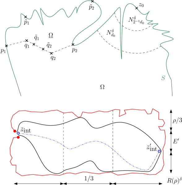
Figure 2. (Top) Settings for the two estimates in Section 4.3. (Bottom) Setting for the analysis of Section 4.4.

4.4. Analysis of the Degenerate Observable

Applying the estimates from previous sections, we derive estimates of the ’degenerate’ $2$-point observable which are crucial in proving Theorem 1.3. We undertake it here since it may be done without identifying a unique continuum scaling limit.

Fix a rectangle $R=R(\rho):=\left(0,1\right)+\left(0,\rho i\right)$ which we discretise and give the FK-Ising measure with entirely wired boundary condition. Then for any boundary rhombus $\left\langle\underline{z}_{\text{int}}u_{1}\underline{z}_{\text{ext}}u_{2}\right\rangle$ on the segment $\left[\left(\frac{2\rho i}{3}\right)^{\delta},\left(\frac{\rho i}{3}\right)^{\delta}\right]$ with inner dual vertex $\underline{z}_{\text{int}}$, we can consider the degenerate $2$-point observable $F_{\underline{z}_{\text{int}}}^{\delta}:=F_{\left(R^{\delta},a^{\delta},b^{\delta}\right)}^{\delta}$ where $a^{\delta}=\left\langle u_{1}\underline{z}_{\text{int}}\right\rangle$ and $b^{\delta}=\left\langle u_{2}\underline{z}_{\text{int}}\right\rangle$. Clearly, this 2-point Dobrushin model on $\left(R^{\delta},a^{\delta},b^{\delta}\right)$ is identical to the fully wired one (see Figure 2B). By definition, for any other boundary rhombus $\left\langle\underline{z}_{\text{int}}^{\prime}u_{1}^{\prime}\underline{z}_{\text{ext}}^{\prime}u_{2}^{\prime}\right\rangle$, evaluating $F^{\delta}$ at the boundary corners $\left\langle u_{1,2}^{\prime}\underline{z}_{\text{int}}^{\prime}\right\rangle$ simply gives the dual-crossing probability

(4.15) $$\left|F_{\underline{z}_{\text{int}}}^{\delta}\left(\left\langle u_{1,2}^{\prime}\underline{z}_{\text{ext}}^{\prime}\right\rangle\right)\right|=\mathbb{P}\left[\underline{z}{}_{\text{int}}\xleftrightarrow{\text{d}}\underline{z}^{\prime}_{\text{int}}\right].$$

Because $a^{\delta}$ and $b^{\delta}$ are $O(\delta)$-apart, the function $F_{\underline{z}_{\text{int}}}^{\delta}$ scales differently from the usual non-degenerate 2-point observable. In this setting, the boundary values of the square integral $H_{\underline{z}_{\text{int}}}^{\delta}$ may be chosen to be all zero except at the dual vertex $\underline{z}_{\text{int}}$, where $H_{\underline{z}_{\text{int}}}^{\delta}(\underline{z}_{\text{int}})=-2\delta$. Thinking of continuum Poisson kernel (i.e. in the massless case), it makes sense to renormalise $H_{\underline{z}}^{\delta}$ by $\delta^{-2}$ to obtain a nontrivial limit, i.e. $F_{\underline{z}_{\text{int}}}^{\delta}$ scales like $\delta$ away from $\underline{z}_{\text{int}}$. We show below that this intuition yields some correct bounds (in terms of the magnitude) at least for small mass; we will carry out more general analysis of $F_{\underline{z}_{\text{int}}}^{\delta}$ (which coincides with the martingale observable for the spin-Ising interface started at $\underline{z}_{\text{int}}$) in [CPW22].

First we show an upper bound for the discrete $L^{1}$-norm of $H_{\underline{z}_{\text{int}}}^{\delta}$.

Lemma 4.11.

There exists some $m_{1}=m_{1}(\eta,\rho),\operatorname{C}(\rho,\eta)>0$ such that, at $m\leq m_{1}$, for any $\underline{z}_{\text{int}}$ on $\left[\left(\frac{2\rho i}{3}\right)^{\delta},\left(\frac{\rho i}{3}\right)^{\delta}\right]$,

(4.16) $$0\leq-\sum_{w\in\Gamma^{*}\left(R^{\delta}\right)}\mu_{\Gamma^{*}}^{\delta}(w)H_{\underline{z}_{\text{int}}}^{\delta}(w)\leq\operatorname{C}(\rho,\eta)\delta^{2}.$$

Proof.

We decompose $H_{\underline{z}_{\text{int}}}^{\delta}$ (and not its square, as we have done throughout most of this paper) on the dual graph $\Gamma^{*}$ into its harmonic and non-harmonic parts:

$$H_{\underline{z}_{\text{int}}}^{\delta}(w)=-2\delta\cdot\omega^{\delta}\left(w,\left\{\underline{z}_{\text{int}}\right\},\Gamma^{*}\left(R^{\delta}\right)\right)+\sum_{w^{\prime}\in\Gamma^{*}\left(R^{\delta}\right)}\mu_{\Gamma^{*}}^{\delta}(w^{\prime})G_{\Gamma^{*}\left(R^{\delta}\right)}^{\delta}(w,w^{\prime})\Delta^{\delta}H_{\underline{z}_{\text{int}}}^{\delta}(w^{\prime}).$$

We analyse the two terms separately.

First, we have the standard estimate $\omega^{\delta}\left(w,\left\{\underline{z}_{\text{int}}\right\},\Gamma^{*}\left(R^{\delta}\right)\right)\apprle\frac{\delta}{\left|w-\underline{z}_{\text{ext}}\right|}$. A simple derivation using discrete comparison principle goes as follows: RHS is (continuum) subharmonic, so in view of [ChSm11, Lemma 2.2(ii)], it is discrete subharmonic on points $w$ such that $\left|w-\underline{z}_{\text{ext}}\right|\geq\operatorname{C}(\eta)\delta$ for some $\operatorname{C}(\eta)>0$; LHS is zero on $\partial\Gamma^{*}\left(R^{\delta}\right)\setminus\left\{\underline{z}_{\text{int}}\right\}$ and may be bounded by a constant multiple of RHS if $\left|w-\underline{z}_{\text{ext}}\right|\leq\operatorname{C}(\eta)\delta$ in any case since it is globally bounded by $1$. Given this pointwise estimate, we get by integration

$$\sum_{w\in\Gamma^{*}\left(R^{\delta}\right)}\mu_{\Gamma^{*}}^{\delta}(w)\omega^{\delta}\left(w,\left\{\underline{z}_{\text{int}}\right\},\Gamma^{*}\left(R^{\delta}\right)\right)\leq\operatorname{C}(\rho,\eta)\delta,$$

as desired.

For the second term,

$$0\leq-\sum_{w\in\Gamma^{*}\left(R^{\delta}\right)}\mu_{\Gamma^{*}}^{\delta}(w)\sum_{w^{\prime}\in\Gamma^{*}\left(R^{\delta}\right)}\mu_{\Gamma^{*}}^{\delta}(w^{\prime})G_{\Gamma^{*}\left(R^{\delta}\right)}^{\delta}(w,w^{\prime})\Delta^{\delta}H_{\underline{z}_{\text{int}}}^{\delta}(w^{\prime})$$

$$\leq\sum_{w^{\prime}\in\Gamma^{*}\left(R^{\delta}\right)}\mu_{\Gamma^{*}}^{\delta}(w^{\prime})\sum_{w\in\Gamma^{*}\left(R^{\delta}\right)}\mu_{\Gamma^{*}}^{\delta}(w)\left|G_{\Gamma^{*}\left(R^{\delta}\right)}^{\delta}(w,w^{\prime})\right|\max\left(0,\Delta^{\delta}H_{\underline{z}_{\text{int}}}^{\delta}(w^{\prime})\right)$$

$$\leq(1+\rho)\sum_{w^{\prime}\in\Gamma^{*}\left(R^{\delta}\right)}\mu_{\Gamma^{*}}^{\delta}(w^{\prime})\operatorname{dist}\left(w^{\prime},\partial R\right)\max\left(0,\Delta^{\delta}H_{\underline{z}_{\text{int}}}^{\delta}(w^{\prime})\right),$$

by (4.5). Write $d(w^{\prime}):=\operatorname{dist}\left(w^{\prime},\partial R\right)$, and let us now show

$$\sum_{w^{\prime}\in\Gamma^{*}\left(R^{\delta}\right)}\mu_{\Gamma^{*}}^{\delta}(w^{\prime})d(w^{\prime})\max\left(0,\Delta^{\delta}H_{\underline{z}_{\text{int}}}^{\delta}(w^{\prime})\right)$$

(4.17) $$\apprle m\left(m(1+\rho)\delta^{2}+(1+m^{2}(1+\rho^{2}))^{3}\sum_{w^{\prime}\in\Gamma^{*}\left(R^{\delta}\right)}\mu_{\Gamma^{*}}^{\delta}(w^{\prime})\left|H_{\underline{z}_{\text{int}}}^{\delta}(w^{\prime})\right|\right),$$

given which we may clearly restrict to small enough $m$ to obtain (4.16). We estimate the Laplacian using (4.7): for $d(w^{\prime})<2\operatorname{C}\delta$ as in Proposition 4.6, there are $(1+\rho)O(\delta^{-1})$ such terms, so the trivial bound from (2.4) and $-2\delta\leq H_{\underline{z}_{\text{int}}}^{\delta}(w)\leq 0$ yields the first term in the bound. If $d(w^{\prime})\geq 2\operatorname{C}\delta$, we have again from (4.7) and Proposition 4.6

$$\frac{\operatorname{dist}\left(w^{\prime},\partial R\right)\Delta^{\delta}H_{\underline{z}_{\text{int}}}^{\delta}(w^{\prime})}{m(1+m^{2}(1+\rho^{2}))^{3}} \apprle\frac{\sum_{w\in\Gamma^{*}\left(B_{d(w^{\prime})}^{\delta}(w^{\prime})\right)}\mu_{\Gamma^{*}}^{\delta}(w)\left|H_{\underline{z}_{\text{int}}}^{\delta}(w)\right|}{d(w^{\prime})^{2}},$$

and therefore the area integral of LHS is bounded, up to a universal factor, by the integral of $\left|H_{\underline{z}_{\text{int}}}^{\delta}(w)\right|=-H_{\underline{z}_{\text{int}}}^{\delta}(w)$ by Hardy-Littlewood maximal theorem [Ste82] (say, apply to the piecewise constant extension of $H_{\underline{z}_{\text{int}}}^{\delta}$ to each face in $\Gamma^{*}$). Therefore the proof is finished. ∎

Preceding integral estimate can easily be improved to the following pointwise bound.

Lemma 4.12.

There exists $0<m_{2}=m_{2}(\rho,\eta)\leq m_{1}$, such that at $m\leq m_{2}$, for any fixed $\beta\in\left(0,1\right)$,

$$-\operatorname{C}\left(\beta,\rho\right)\delta^{2}\apprle\min\left\{H_{\underline{z}_{\text{int}}}^{\delta}(w):\operatorname{Re}w\in\left(\beta-2\delta,\beta+2\delta\right)\right\},$$

for some $\operatorname{C}\left(\beta,\rho\right)>0$.

Proof.

Write $\min(\beta):=\min\left\{H_{\underline{z}_{\text{int}}}^{\delta}(w):\operatorname{Re}w\in\left(\beta-2\delta,\beta+2\delta\right)\right\}$. By minimum principle, there is a nearest-neighbour path $l^{\delta}$ of dual vertices from some $w_{0}$ with $\operatorname{Re}w_{0}\in\left(\beta-2\delta,\beta+2\delta\right)$ which ends at $\underline{z}_{\text{int}}$ along which $H_{\underline{z}_{\text{int}}}^{\delta}\leq\min(\beta)$. Then on $\Gamma^{*}\left(R^{\delta}\right)\setminus l^{\delta}$, we again have the decomposition

$$H_{\underline{z}_{\text{int}}}^{\delta}(w) \leq\min(\beta)\cdot\omega^{\delta}\left(w,l^{\delta},\Gamma^{*}\left(R^{\delta}\right)\setminus l^{\delta}\right)$$

$$+\sum_{w^{\prime}\in\Gamma^{*}\left(R^{\delta}\right)\setminus l^{\delta}}\mu_{\Gamma^{*}}^{\delta}(w^{\prime})G_{\Gamma^{*}\left(R^{\delta}\right)\setminus\omega^{\delta}}^{\delta}(w,w^{\prime})\Delta^{\delta}H_{\underline{z}_{\text{int}}}^{\delta}(w^{\prime}).$$

Again let us consider the area integral of the involved functions:

• The integral of $H_{\underline{z}_{\text{int}}}^{\delta}(w)$ is bounded below by $-\operatorname{C}(\rho,\eta)\delta^{2}$ by (4.16).

• It is clear from standard harmonic function estimates [ChSm11, Proposition 2.11] that the integral of $\omega^{\delta}\left(w,l^{\delta},\Gamma^{*}\left(R^{\delta}\right)\setminus l^{\delta}\right)$ is bounded below by some $\operatorname{c}(\beta,\rho,\eta)>0$.

• Since $G_{\Gamma^{*}\left(R^{\delta}\right)\setminus l^{\delta}}^{\delta}(w,w^{\prime})\geq G_{\Gamma^{*}\left(R^{\delta}\right)}^{\delta}(w,w^{\prime})$, we have

  $$\sum_{w^{\prime}\in\Gamma^{*}\left(R^{\delta}\right)\setminus\omega^{\delta}}\mu_{\Gamma^{*}}^{\delta}(w^{\prime})G_{\Gamma^{*}\left(R^{\delta}\right)\setminus\omega^{\delta}}^{\delta}(w,w^{\prime})\Delta^{\delta}H_{\underline{z}_{\text{int}}}^{\delta}(w^{\prime})$$

  $$\geq\sum_{w^{\prime}\in\Gamma^{*}\left(R^{\delta}\right)}\mu_{\Gamma^{*}}^{\delta}(w^{\prime})G_{\Gamma^{*}\left(R^{\delta}\right)}^{\delta}(w,w^{\prime})\max\left(0,\Delta^{\delta}H_{\underline{z}_{\text{int}}}^{\delta}(w^{\prime})\right),$$

  and the area integral of RHS is bounded below by some other $-m\operatorname{C}(\rho,\eta)\delta^{2}$ by (4.17) and (4.16).

Given the above three bounds, we clearly have $\min(\beta)\geq-\operatorname{C}\left(\beta,\rho\right)\delta^{2}$ if $m$ is small enough. ∎

We are ready to give the needed lower bound on the crossing expectation:

Corollary 4.13.

There exists some $m_{0}=m_{0}(\rho,\eta),\operatorname{c}(\rho,\eta)>0$ such that, at $m\leq m_{0}$, for any $\underline{z}_{\text{int}}$ on $\left[\left(\frac{2\rho i}{3}\right)^{\delta},\left(\frac{\rho i}{3}\right)^{\delta}\right]$,

(4.18) $$\sum_{\underline{z}^{\prime}\in\left[\left(1+\frac{2\rho i}{3}\right)^{\delta},\left(1+\frac{\rho i}{3}\right)^{\delta}\right]}\left|F_{\underline{z}_{\text{int}}}^{\delta}(\underline{z}^{\prime})\right|^{2}\geq\operatorname{c}(\rho,\eta)\delta.$$

As a result, there exists a constant $\operatorname{c}(\rho,\eta)>0$ such that at $m=m_{0}$ we have

(4.19) $$\sum\mathbb{P}\left[\underline{z}_{\text{int}}\xleftrightarrow{\text{d}}\underline{z}^{\prime}{}_{\text{int}}\right]\geq\operatorname{c}\left(\rho,\eta\right)\delta^{-1},$$

summing over $\underline{z}\in\left[\left(\frac{2\rho i}{3}\right)^{\delta},\left(\frac{\rho i}{3}\right)^{\delta}\right],\underline{z}^{\prime}\in\left[\left(1+\frac{2\rho i}{3}\right)^{\delta},\left(1+\frac{\rho i}{3}\right)^{\delta}\right]$.

Proof.

Since $\left(F_{\underline{z}_{\text{int}}}^{\delta}\right)^{2}$ is the discrete (normal) derivative of $H_{\underline{z}_{\text{int}}}^{\delta}$ on the boundary (with modified but uniformly positive weights as in Lemma 2.6) and $H_{\underline{z}_{\text{int}}}^{\delta}\left(\underline{z}^{\prime}_{\text{ext}}\right)=0$, to get (4.18) it suffices to show

$$\sum_{\underline{z}^{\prime}\in\left[\left(1+\frac{2\rho i}{3}\right)^{\delta},\left(1+\frac{\rho i}{3}\right)^{\delta}\right]}H_{\underline{z}_{\text{int}}}^{\delta}(\underline{z}^{\prime}_{\text{int}})\leq-\operatorname{c}(\rho,\eta)\delta^{2}.$$

By (2.3), we may instead show this on the primal vertices, i.e. write $E^{\prime}$ for the set of the boundary primal vertices on $\left[\left(1+\frac{2\rho i}{3}\right)^{\delta},\left(1+\frac{\rho i}{3}\right)^{\delta}\right]$, and show

(4.20) $$\sum_{u\in\Gamma\left(R^{\delta}\right),u\sim E^{\prime}}H_{\underline{z}_{\text{int}}}^{\delta}(u)\leq-\operatorname{c}(\rho,\eta)\delta^{2}.$$

While the value of $H_{\underline{z}_{\text{int}}}^{\delta}$ on $\partial\Gamma\left(R^{\delta}\right)$ is identically zero, there is always some $u_{0}\subset\Gamma\left(R^{\delta}\right)$ such that $\left|u_{0}-\underline{z}_{\text{int}}\right|\leq 4\delta$ where $H_{\underline{z}_{\text{int}}}^{\delta}(u_{0})\leq-\operatorname{c}\left(\rho,\eta\right)\delta$: if not, for any primal vertex $u$ incident to $\underline{z}_{\text{int}}$, we would have $\sum_{z\sim u}\left|\partial^{\delta}H_{\underline{z}_{\text{int}}}^{\delta}|_{\Gamma}(z)\right|=o(1)$, which contradicts (4.8) since the corner value $\left|F_{\underline{z}_{\text{int}}}^{\delta}\right|^{2}\left(u\underline{z}_{\text{int}}\right)=1-o(1)$ by assumption. Applying discrete Green’s formula (4.3) on $H_{\underline{z}_{\text{int}}}^{\delta}$ and the harmonic measure $V:=\omega^{\delta}\left(\cdot,E^{\prime},\Gamma\left(R^{\delta}\setminus\left\{u_{0}\right\}\right)\right)$ on $\Gamma\left(R^{\delta}\setminus\left\{u_{0}\right\}\right)$,

$$\sum_{u\in\Gamma(R^{\delta})\setminus\left\{u_{0}\right\}}\left[-V\Delta^{\delta}H_{\underline{z}_{\text{int}}}^{\delta}\right](u)\mu_{\Gamma}^{\delta}\left(u\right)$$

$$=\sum_{u\sim u_{\text{ext}}\in E^{\prime}}t_{(uu_{\text{ext}})}\cdot\left[H_{\underline{z}_{\text{int}}}^{\delta}(u)\right]-H_{\underline{z}_{\text{int}}}^{\delta}(u_{0})\sum_{u\sim u_{0}}t_{\left(uu_{0}\right)}V(u).$$

Again by standard estimates [ChSm11, Lemma 3.17] and since $t\apprge 1$, we have $\sum_{u\sim u_{0}}t_{\left(uu_{0}\right)}V(u)\geq\operatorname{c}(\rho,\eta)\delta$. We will now show that LHS is bounded above by $m\operatorname{C}(\rho,\eta)\delta^{2}$, so that we may set small enough $m$ to get (4.20).

We analyse the LHS by dividing $\left(0,1\right)\ni\operatorname{Re}u$ into two pieces. Again it is easy to deduce from [ChSm11, Lemma 3.17] that $V(u)\leq\operatorname{C}\left(\rho,\eta\right)\operatorname{dist}\left(u,\partial R\right)$ for $\operatorname{Re}u<\frac{2}{3}$. Therefore, for small $m$,

$$\sum_{\operatorname{Re}u<\frac{2}{3}}\left[-V\Delta^{\delta}H_{\underline{z}_{\text{int}}}^{\delta}\right](u)\mu_{\Gamma}^{\delta}\left(u\right)\leq m\operatorname{C}(\rho,\epsilon)\delta^{2},$$

where we essentially repeat the proof of (4.17) but on $\Gamma$, with the lower bound (4.6). The required $O(\delta^{2})$ area integral bound directly comes from (4.16), since the bound on $\Gamma^{*}$ bounds the area integral on $\Gamma$ from (2.3).

For the bound for $\operatorname{Re}u\geq\frac{2}{3}$, note that $\operatorname{osc}_{\operatorname{Re}u\geq\frac{1}{3}}H_{\underline{z}_{\text{int}}}^{\delta}\leq\operatorname{C}\left(\beta=\frac{1}{3},\rho,\epsilon\right)\delta^{2}$ from Lemma 4.12. By Remark 4.9 and Proposition 4.6, $\left|F_{\underline{z}_{\text{int}}}^{\delta}(z)\right|^{2}\leq\operatorname{C}\left(\rho,\epsilon\right)\delta^{2}$ if $\operatorname{Re}z\geq\frac{2}{3}$. Again using (4.6) and bounding $V\leq 1$, we have $\sum_{\operatorname{Re}u\geq\frac{2}{3}}\left[-V\Delta^{\delta}H_{\underline{z}_{\text{int}}}^{\delta}\right](u)\mu_{\Gamma}^{\delta}\left(u\right)\leq m\operatorname{C}(\rho,\epsilon)\delta^{2}$.

Therefore (4.20) holds for small $m$. Since $\left|F_{\underline{z}_{\text{int}}}^{\delta}(\underline{z}^{\prime})\right|\leq\sqrt{\operatorname{C}\left(\rho,\epsilon\right)}\delta$ as noted above, we have (4.19) given (4.15). ∎

5. Continuum Observable

5.1. How do the Continuum Observables Look?

In this descriptive section, we define and illustrate the continuous limits of the discrete observables defined in Section 2.1 and their square integrals; the proofs of their uniqueness (and therefore convergence and existence) will be given in the next section. We will consider observables corresponding to two masses: massive $m>0$ (assumed to be fixed and implicit) and the massless case $m=0$ (marked by an explicit superscript). They will turn out to be related by (up to constant factors) exactly the factorisation in Definition 3.4.

In the massless case, the square integrals are harmonic and thus may be identified by their boundary values, which are locally constant. Therefore, they are a linear combination of harmonic measures (cf., e.g. [GaMa08])

Theorem 5.1 ([ChSm12, Theorem 4.3]).

In the massless case, the $2$-point observable (Definition 2.1 with $q=0$) converges to a holomorphic function $f_{\left(\Omega,a,b\right)}^{m=0}$, unique up to a sign, satisfying the following:

• for any conformal pullback $D\xrightarrow{\varphi}\Omega$, pullback $f_{\left(\Omega,a,b\right)}^{\text{pb};m=0}=\left(f_{\left(\Omega,a,b\right)}^{m=0}\circ\varphi\right)\cdot\left(\varphi^{\prime}\right)^{1/2}$ coincides with the observable $f_{\left(D,\varphi^{-1}(a),\varphi^{-1}(b)\right)}^{m=0}$ , i.e. the observable is conformally covariant;

• $f_{\left(D,\varphi^{-1}(a),\varphi^{-1}(b)\right)}^{m=0}$ satisfies $(rh)_{f}$, and in particular is smooth away from $\varphi^{-1}(a),\varphi^{-1}(b)$;

• square integral $h_{\left(\Omega,a,b\right)}^{m=0}:=\operatorname{Im}\int\left(f_{\left(\Omega,a,b\right)}^{m=0}\right)^{2}dz$ is conformally invariant, i.e. $h_{\left(\Omega,a,b\right)}^{m=0}=h_{\left(D,\varphi^{-1}(a),\varphi^{-1}(b)\right)}^{m=0}\circ\varphi$;

• the harmonic function $h_{\left(\Omega,a,b\right)}^{m=0}(z)$ coincides with $\omega\left(z,\left(ba\right),\Omega\right)$, the harmonic measure of $(ba)\subset\partial\Omega$ seen from $z$, characterised by

  $$h_{\left(\Omega,a,b\right)}^{m=0}=0\text{ on }\left(ab\right)\text{, }h_{\left(\Omega,a,b\right)}^{m=0}=1\text{ on }\left(ba\right);$$

• on the strip $\mathbb{S}:=\mathbb{R}+\left(0,i\right)$, we have explicit observables $f_{\left(\mathbb{S},-\infty,\infty\right)}^{m=0}\equiv 1$ and $h_{\left(\mathbb{S},-\infty,\infty\right)}^{m=0}(x+yi)=y$.

Accordingly, we define the continuous massive observable as the function satisfying the following, shown to be unique in the next subsection.

Definition 5.2.

Given the $2$-point marked domain $\left(\Omega,a,b\right)$, the continuous $2$-point observable $f_{\left(\Omega,a,b\right)}$ is the massive holomorphic function, unique up to a sign, having the following properties:

• $f_{\left(\Omega,a,b\right)}$ satisfies $(rh)_{f}$;

• square integral $h_{\left(\Omega,a,b\right)}:=\operatorname{Im}\int\left(f_{\left(\Omega,a,b\right)}\right)^{2}dz$ is a solution of $\Delta h_{\left(\Omega,a,b\right)}=-4m\left|\nabla h_{\left(\Omega,a,b\right)}\right|$;

• $h_{\left(\Omega,a,b\right)}(z)$ has the following boundary values

  $$h_{\left(\Omega,a,b\right)}\equiv 0\text{ on }\left(ab\right)\text{, }h_{\left(\Omega,a,b\right)}\equiv 1\text{ on }\left(ba\right);$$

• holomorphic parts $\underline{f}_{\left(\Omega,a,b\right)},\underline{f}_{\left(\Omega,a,b\right)}^{\text{pb}}$ respectively coincide with $f_{\left(\Omega,a,b\right)}^{m=0},f_{\left(D,\varphi^{-1}(a),\varphi^{-1}(b)\right)}^{m=0}$ up to real multiplicative constants.

Remark 5.3.

Near the points $a,b$, where $h_{\left(\Omega,a,b\right)}^{m=0}$ has a jump discontinuity, the conformal invariance allows us to deduce $f_{\left(\Omega,a,b\right)}^{m=0}(z)$ has series expansions in half-integers with leading inverse square root poles, in any simply connected domain $\Omega$ in the case where the prime ends $a,b$ are single accessible points. The fact that in the massive case there has to be some blow-up in inverse square root rate may be deduced from the mean value theorem (from below) and Proposition 3.9 (from above).

Theorem 5.4 ([ChSm12, Proof of Theorem 6.1]).

In the massless case, the $4$-point observable (Definition 2.4 with $q=0$) converges to a holomorphic function $f_{\left(\Omega,a,b,c,d\right)}^{m=0}$, unique up to a sign, satisfying the following:

• analogues of the first three properties in Theorem 5.1;

• the harmonic function $h_{\left(\Omega,a,b,c,d\right)}^{m=0}$ has the boundary values

  (5.1) $$h_{\left(\Omega,a,b,c,d\right)}^{m=0}\equiv 0\text{ on }\left(ab\right)\text{, }h_{\left(\Omega,a,b,c,d\right)}^{m=0}\equiv 1\text{ on }\left(bc\right),h_{\left(\Omega,a,b,c,d\right)}^{m=0}\equiv\varkappa_{m=0}\text{ on }\left(ca\right),$$

  where $\varkappa_{m=0}\in\left(0,1\right)$ is the conformally invariant unique value which realises $(rh)_{h}$ for $h_{\left(\Omega,a,b,c,d\right)}^{m=0}$;

• on the slit-strip $\mathbb{S}_{\varkappa_{m=0}}:=\mathbb{S}\setminus\left(\mathbb{R}_{<0}+\varkappa_{m=0}i\right)$, we have the explicit observables

  $$f_{\left(\mathbb{S}_{\varkappa_{m=0}},-\infty+0\cdot i,+\infty,-\infty+i,\varkappa_{m=0}i\right)}^{m=0}\equiv 1,h_{\left(\mathbb{S}_{\varkappa_{m=0}},-\infty+0\cdot i,+\infty,-\infty+i,\varkappa_{m=0}i\right)}^{m=0}(x+yi)=y.$$

And we have

Definition 5.5.

Given the $4$-point marked domain $\left(\Omega,a,b,c,d\right)$, the continuous $2$-point observable $f_{\left(\Omega,a,b,c,d\right)}$ is the massive holomorphic function, unique up to a sign, having the following properties:

• pullback $f_{\left(\Omega,a,b,c,d\right)}^{\text{pb}}$ on any $D$ satisfies $(rh)_{f}$;

• square integral $h_{\left(\Omega,a,b,c,d\right)}:=\operatorname{Im}\int\left(f_{\left(\Omega,a,b,c,d\right)}\right)^{2}dz$ is a solution of $\Delta h_{\left(\Omega,a,b,c,d\right)}=-4m\left|\nabla h_{\left(\Omega,a,b,c,d\right)}\right|$;

• $h_{\left(\Omega,a,b,c,d\right)}(z)$ has the following boundary values

  $$h_{\left(\Omega,a,b,c,d\right)}\equiv 0\text{ on }\left(ab\right)\text{, }h_{\left(\Omega,a,b,c,d\right)}\equiv 1\text{ on }\left(bc\right),h_{\left(\Omega,a,b,c,d\right)}\equiv\varkappa_{m}\text{ on }\left(ca\right),$$

  where $\varkappa_{m}\in\left(0,1\right)$ is the unique value which realises $(rh)_{h}$ for $h_{\left(\Omega,a,b,c,d\right)}$;

• holomorphic parts $\underline{f}_{\left(\Omega,a,b,c,d\right)},\underline{f}_{\left(\Omega,a,b,c,d\right)}^{\text{pb}}$ respectively coincide with $f_{\left(\Omega,a,b,c,d\right)}^{m=0},f_{\left(D,\varphi^{-1}(a),\varphi^{-1}(b),\varphi^{-1}(c),\varphi^{-1}(d)\right)}^{m=0}$ up to real multiplicative constants.

Remark 5.6.

If the boundary arc near $d$ is smooth, it is easy to see that massless $\left(f_{\left(\Omega,a,b,c,d\right)}^{m=0}\right)^{2}$ has a simple zero at $d$. Unlike the jump discontinuities at $a,b$, regularity of the boundary is important; e.g. there is no zero if $d$ is the endpoint of an inward slit.

5.2. $2$-Point Observable and Improved Regularity

We now identify the limit $f_{\left(\Omega,a,b\right)}$ of the $2$-point observables as the unique function satisfying the conditions set out in Definition 5.2. First, we will prove uniqueness of the solution of the PDE given the boundary values, which any subsequential limit of the two-point observable (or rather, the square integral thereof) satisfies. Then, given uniqueness and therefore convergence, we will be able to also characterise the function in terms of the factorisation of Definition 3.4, which improves the boundary regularity.

We first state the following standard lemma.

Lemma 5.7.

Let $G_{\Omega}$ be the Green’s function for the Dirichlet Laplacian on $\Omega$. If for some $\alpha>0$, a locally Hölder function $g$ on $\Omega$ satisfies the estimate $\left|g(z)\right|=O({\operatorname{dist}(z,\partial\Omega)^{2-\alpha}})$, then

$$\Phi(z):=\iint_{\Omega}G_{\Omega}(z,z^{\prime})g(z^{\prime})d^{2}z^{\prime}$$

is twice differentiable, solves the Poisson’s equation $\Delta\Phi=g$, and takes the boundary value $0$ continuously.

Proof.

The proof of [Che20, Lemma A.2] proves the boundedness and (Hölder) continuity up to boundary of the RHS. The (local) twice differentiability and the resulting Laplacian is a standard result, e.g. using [GiTr15, Lemma 4.2]. ∎

The following proposition shows that any subsequential limit of $F_{\left(\Omega^{\delta},a^{\delta},b^{\delta}\right)}^{\delta}$ obtained by Remark 4.7 has to be unique, therefore completing the proof of convergence.

Proposition 5.8.

Any limit $f_{\left(\Omega,a,b\right)}$ of $F_{\left(\Omega^{\delta},a^{\delta},b^{\delta}\right)}^{\delta}$ has a square integral $h_{\left(\Omega,a,b\right)}$ which is the unique solution to the boundary value problem in Definition 5.2, and is therefore unique up to a sign.

Proof.

Suppose there are two solutions $f_{\left(\Omega,a,b\right)}^{1,2}$ with two square integrals $h_{\left(\Omega,a,b\right)}^{1,2}$ continuously taking the boundary value on each open boundary arc by Proposition 4.8. We have that

$$\left|f_{\left(\Omega,a,b\right)}^{1,2}(z)\right|^{2}=O({\operatorname{dist}(z,\partial\Omega)}^{-1}),$$

by Proposition 3.9 (or, simply by the fact that the discrete estimate from Proposition 4.6 used for precompactness is inherited). Then define

$$\Phi(z):=\iint_{\Omega}-4m\left(\left|f_{\left(\Omega,a,b\right)}^{1}(w)\right|^{2}-\left|f_{\left(\Omega,a,b\right)}^{2}(w)\right|^{2}\right)G_{\Omega}(z,w)d^{2}w,$$

which has the same Laplacian as $h_{\left(\Omega,a,b\right)}^{1}-h_{\left(\Omega,a,b\right)}^{2}$ and takes zero boundary value everywhere on $\partial\Omega$ by Lemma 5.7. Therefore, $h_{\left(\Omega,a,b\right)}^{1}-h_{\left(\Omega,a,b\right)}^{2}-\Phi$ is a bounded harmonic function continuously taking zero boundary value on $\partial\Omega\setminus\{a,b\}$; since $a,b$ are isolated prime ends, there is no such nonzero harmonic function (e.g. [GaMa08, Lemma 1.1]). So $h_{\left(\Omega,a,b\right)}^{1}-h_{\left(\Omega,a,b\right)}^{2}$ continuously takes zero boundary value everywhere on $\partial\Omega$, and by comparison principle (Lemma 3.6) $h_{\left(\Omega,a,b\right)}^{1}=h_{\left(\Omega,a,b\right)}^{2}$ everywhere. ∎

Remark 5.9.

The above proof illustrates how Lemma 5.7 implies that, analogously to the harmonic case, bounded massive holomorphic integrals $h$ cannot be supported on discrete prime ends, since they do not have enough capacity. This in particular justifies only specifying boundary values of square integrals on open boundary arcs, missing a finite number of prime ends.

Now we identify $f_{\left(\Omega,a,b\right)}$ as precisely the function whose holomorphic part comes from the corresponding boundary value problem in the massless case.

Corollary 5.10.

The holomorphic part $\underline{f}_{\left(\Omega,a,b\right)}$ of $f_{\left(\Omega,a,b\right)}$ as defined in Definition 3.4 coincides with $f_{\left(\Omega,a,b\right)}^{m=0}$ up to a real multiplicative constant, which satisfies

$$\operatorname{c}\left(m\operatorname{diam}\Omega\right)\leq\left(f_{\left(\Omega,a,b\right)}^{m=0}/\underline{f}_{\left(\Omega,a,b\right)}\right)^{2}\leq\operatorname{C}\left(m\operatorname{diam}\Omega\right),$$

i.e. positive constants only depending on $m\operatorname{diam}\Omega$. In particular, $\underline{f}_{\left(\Omega,a,b\right)}$ satisfies $(rh)_{f}$ on $\partial\Omega\setminus\left\{a,b\right\}$.

Proof.

Exploiting uniqueness of the factorisation (3.3), we may show this in the opposite order: i.e. $f_{\left(\Omega,a,b\right)}^{m=0}$ has a massive holomorphic counterpart $g$ as in Definition 3.4 such that $\underline{g}=f_{\left(\Omega,a,b\right)}^{m=0}$. But by Propositions A.9 and A.10, the square integral $i(z):=\operatorname{Im}\int^{z}g^{2}dz$ satisfies $(rh)_{h}$ on $(ab)$ and $(ba)$: it is easy then to see that it has to coincide with $h_{\left(\Omega,a,b\right)}$ up to additive and positive multiplicative constants.

Consequently,

(5.2) $$g=kf_{\left(\Omega,a,b\right)}\text{ for some }k\in\mathbb{R}.$$

Also note that

$$i\left(ba\right)-i\left(ab\right)=k^{2}\left(h_{\left(\Omega,a,b\right)}\left(ba\right)-h_{\left(\Omega,a,b\right)}\left(ab\right)\right)=k^{2}.$$

To estimate $k^{2}$, we pullback to the unit disc: fix a map $\varphi_{\mathbb{D}}:\mathbb{D}\to\Omega$ such that $\varphi_{\mathbb{S}}(i)=a,\varphi_{\mathbb{S}}(-i)=b$. On the truncated disc $\mathbb{D}\cap\left\{z:\left|\operatorname{Im}z\right|\leq\frac{1}{2}\right\}$, we have the universal bounds $0<\operatorname{c}\leq\left|f_{\left(\mathbb{D},i,-i\right)}^{m=0}\right|\leq\operatorname{C}$ : pullback to the strip is identically $1$ from Theorem 5.1, and any fixed map from the disc to the strip mapping $\mp\infty$ to $\pm i$ also satisfies the same lower/upper bounds.

Then as usual the pullback of $g$ and $i$ becomes simply

$$g_{\mathbb{D}}:=\left(g\circ\varphi_{\mathbb{D}}\right)\cdot\left(\varphi_{\mathbb{D}}^{\prime}\right)^{1/2}\text{, and }i\circ\varphi_{\mathbb{D}}^{-1}=\operatorname{Im}\int g_{\mathbb{D}}^{2}dz.$$

Recall the massless observable is conformally covariant, so that $g_{\mathbb{D}}=e^{s_{g_{\mathbb{D}}}^{\mathbb{D}}}f_{\left(\mathbb{D},i,-i\right)}^{m=0}$ with $\left\|s_{g_{\mathbb{D}}}^{\mathbb{D}}\right\|_{W^{1,2}\left(\mathbb{D}\right)}\leq\operatorname{C}m\operatorname{diam}\Omega$. So we apply Lemma A.8 to bound $k^{2}=\operatorname{Im}\int_{-1}^{1}\left(e^{s_{g_{\mathbb{D}}}^{\mathbb{D}}}f_{\left(\mathbb{D},i,-i\right)}^{m=0}\right)^{2}dz\leq\operatorname{C}\left(m\operatorname{diam}\Omega\right)$.

For the lower bound, take the holomorphic parts of both sides of (5.2) and pullback to $\mathbb{S}$. We get $\left(\underline{f}_{\left(\Omega,a,b\right)}\circ\varphi_{\mathbb{S}}\right)\cdot\left(\varphi_{\mathbb{S}}^{\prime}\right)^{1/2}=k^{-1}f_{\left(\mathbb{D},i,-i\right)}^{m=0}$. Applying Proposition 3.9 on the massive holomorphic pullback $f_{\left(\Omega,a,b\right)}^{\text{pb}}$ and its square integral $h_{\left(\Omega,a,b\right)}^{\text{pb }}$ (whose oscillation is bounded above by $1$) on $\mathbb{D}$, we have on $B_{1/4}(0)\subset\mathbb{D}$

$$\left|f_{\left(\Omega,a,b\right)}^{\text{pb}}\right|=\left|e^{s_{f_{\left(\Omega,a,b\right)}^{\text{pb}}}^{\mathbb{D}}}\underline{f}_{\left(\Omega,a,b\right)}^{\text{pb}}\right|=\left|k^{-1}e^{s_{f_{\left(\Omega,a,b\right)}^{\text{pb}}}^{\mathbb{D}}}f_{\left(\mathbb{D},i,-i\right)}^{m=0}\right|\leq\operatorname{C}.$$

Therefore, taking the $L^{2}$-norm on $B_{1/4}(0)$, we have $k^{-2}\leq\operatorname{C}\left\|e^{s_{f_{\left(\Omega,a,b\right)}^{\text{pb}}}^{\mathbb{D}}}\right\|_{L^{2}\left(B_{1/4}(0)\right)}^{2}\leq\operatorname{C}\left(m\operatorname{diam}\Omega\right)$, applying Lemma A.8. ∎

Figure 3. (Left-top) Setting for the analysis of Theorem 5.11. Top shows some pathologies of the level line (pulled back) $\varphi^{-1}(\omega)$ to be ruled out: self-intersection (rays like the ones in orange are used for the proof of contradiction) and accumulation near an open interval containing $0$. (Left-bottom) Half-balls used in the non-existence proof of the latter. (Right) Simulations of the 4-point square integral $\left.H_{\left(\Omega^{\delta},a,b,c,d\right)}^{\delta}\right|_{\Gamma^{*}}$ on the slit unit square $\Omega:=R(1)\setminus\left(\frac{i}{2},\frac{1+i}{2}\right)$ discretised by hexagonal faces ($8\times 8$, $20\times 20$, $40\times 40$), here rendered as squares. The hue is lighter for greater values, and points in $\left\{H_{\left(\Omega^{\delta},a,b,c,d\right)}^{\delta}\leq\varkappa^{\delta}\right\}$ have slight transparency to delineate the level lines from $b^{\delta}$ to $d^{\delta}$. The mass parameter is set $m=\frac{2\sqrt{3}}{5}\simeq 0.69$.

5.3. Level Set Decomposition and $4$-Point Observable

Again, by Remark 4.7 and Proposition 4.8, we assume some continuous function which has the properties defined in Definition 5.5 is given. We need to show its uniqueness.

Theorem 5.11.

Suppose any limit $f_{\left(\Omega,a,b,c,d\right)}$ of $F_{\left(\Omega^{\delta},a^{\delta},b^{\delta},c^{\delta},d^{\delta}\right)}^{\delta}$, such that the square integral $h_{\left(\Omega,a,b,c,d\right)}$ continuously takes the boundary values (5.1) for some $\varkappa_{m}\in\left[0,1\right]$, is given. Then $\varkappa_{m}\in\left(0,1\right)$, and there are two disjoint simply connected domains $\Omega_{-},\Omega_{+}$ and the image of a locally smooth curve $\omega$ partitioning $\Omega$, defined by

$$\Omega_{-}:=\left\{h_{\left(\Omega,a,b,c,d\right)}<\varkappa_{m}\right\},\Omega_{+}:=\left\{h_{\left(\Omega,a,b,c,d\right)}>\varkappa_{m}\right\},\omega:=\left\{h_{\left(\Omega,a,b,c,d\right)}=\varkappa_{m}\right\}.$$

We have $\partial\Omega_{-}=\left[ab\right]\cup\left[da\right]\cup\omega,\partial\Omega_{+}=\left[bc\right]\cup\left[cd\right]\cup\omega$. That is, the only limit points (therefore endpoints) of $\omega$ in $\partial\Omega$ are $b$ and $d$.

Proof.

Note that by the strong maximum principle, each connected component of $\Omega_{\pm}$ is simply connected. Then following lemmas will together imply the result.

Lemma 5.12.

$\varkappa_{m}\in(0,1)$.

Proof.

Without loss of generality, suppose $\varkappa_{m}=0$. By Proposition 4.10, any prime end in $\left(da\right)$ as a sequence $z_{j}$ converging to it such that $h_{\left(\Omega,a,b,c,d\right)}(z_{j})\leq 0$. Then by the strong maximum principle, $h_{\left(\Omega,a,b,c,d\right)}$ is a constant, which is impossible since $h_{\left(\Omega,a,b,c,d\right)}$ is continuous up to $\left(bc\right)$ where it takes the value $1$. ∎

Lemma 5.13.

We have

(5.3) $$\overline{\Omega_{+}}\cap\left(ab\right),\overline{\Omega_{-}}\cap\left(bc\right) =\emptyset,$$

and $\Omega_{-}$ and $\Omega_{+}$ are connected.

Proof.

Proposition 4.8 and continuity of $h_{\left(\Omega,a,b,c,d\right)}$ up to boundary segments immediately give (5.3).

Let us now prove connectedness. Given any two connected components $\Omega_{+}^{1,2}$ of $\Omega_{+}$, the intersections $\partial\Omega_{+}^{1,2}\cap\left(bc\right)$ cannot be empty: indeed, then, say, the boundary $\partial\Omega_{+}^{1}$ will be a subset of $\left[cb\right]\cup\omega$, on which $h_{\left(\Omega,a,b,c,d\right)}\leq\varkappa_{m}$ (except possibly at $b,c$), and the maximum principle says that $\Omega_{+}^{1}$ is empty. Fix $z_{1}\in\partial\Omega_{+}^{1}\cap\left(bc\right),z_{2}\in\partial\Omega_{+}^{2}\cap\left(bc\right)$, say counterclockwise along $\left(bc\right)$. By Proposition 4.8, there is an open cover of $\left[z_{1}z_{2}\right]$ consisting of $B_{d_{z}}\left(z\right)$ for $z\subset\left[z_{1}z_{2}\right]$ such that $B_{d_{z}}\left(z\right)\cap\Omega\subset\Omega_{+}$. Then

$$\bigcup_{z\in\left[z_{1}z_{2}\right]}B_{d_{z}}\left(z\right)\cap\Omega,$$

is an open connected set (easily seen, e.g., by pulling back to the unit disc $\mathbb{D}$), which is itself connected to $\Omega_{+}^{1},\Omega_{+}^{2}$: they are thus the same connected component. ∎

Lemma 5.14.

The set $\omega$ is locally the image of a smooth simple curve in $\Omega$.

Proof.

Both smoothness and simpleness will come from the fact that $f_{\left(\Omega,a,b,c,d\right)}$ does not vanish on $\omega$, since then $\omega$ is locally the image of an integral curve of $\left(f_{\left(\Omega,a,b,c,d\right)}\right)^{-2}$. Suppose $f_{\left(\Omega,a,b,c,d\right)}$ has an interior zero (say at $z=0\in\omega$).

Then by Remark 3.3 and smoothness, it is locally of the form $f_{\left(\Omega,a,b,c,d\right)}(z)=t(z)z^{n}$ for some nonzero smooth function $t$ and an integer $n>0$. By rotation and rescaling, assume $t(z)=1+O(\left|z\right|)$. We have, for small $r>0$,

$$h_{\left(\Omega,a,b,c,d\right)}(z=re^{\frac{ik\pi}{4n}})-h_{\left(\Omega,a,b,c,d\right)}(0)=\operatorname{Im}\int_{0}^{z}\left(f_{\left(\Omega,a,b,c,d\right)}(z)\right)^{2}dz$$

is strictly positive (i.e. in $\Omega_{+}$) for $k\equiv 1\mod 4$, and strictly negative (i.e. in $\Omega_{-}$) for $k\equiv 3\mod 4$. Consider for small $0<r\leq r_{0}$, four rays

$$re^{\frac{i\pi}{4n}},re^{\frac{3i\pi}{4n}},re^{\frac{5i\pi}{4n}},re^{\frac{7i\pi}{4n}},$$

which are respectively subsets of $\Omega_{+},\Omega_{-},\Omega_{+},\Omega_{-}$. Then there is a simple curve within $\Omega_{-}$ connecting $r_{0}e^{\frac{3i\pi}{4n}},r_{0}e^{\frac{7i\pi}{4n}}$ bypassing the rays. Concatenating the curve with the line segment connecting the two points, we see that the resulting Jordan curve, on which $h_{\left(\Omega,a,b,c,d\right)}\leq\varkappa_{m}$, envelopes one of $r_{0}e^{\frac{i\pi}{4n}},r_{0}e^{\frac{5i\pi}{4n}}\in\Omega_{+}$: by the maximum principle, this is a contradiction. ∎

Lemma 5.15.

We have $\overline{\Omega_{+}}\cap\left(da\right),\overline{\Omega_{-}}\cap\left(cd\right)=\emptyset$. Therefore, the only limit points of $\omega$ in $\partial\Omega$ are $b$ and $d$.

Proof.

The first statement implies the second, since by Proposition 4.10 $\left(da\right)$ and $\left(cd\right)$ are respectively part of $\partial\Omega_{-}$ and $\partial\Omega_{+}$: the only way the intersection can be nonempty is by there being infinitely many values both below and above $\varkappa_{m}$ near those points. On the other hand, by precisely that reason, $b$ and $d$ are already limit points of $\omega$.

Suppose there is a limit point $c^{\prime}$ of $\Omega_{-}$ along $(cd)$: one cannot lie on $(bc)$. Then $c^{\prime}$ is in the intersection of $\partial\Omega_{-}$ and $\partial\Omega_{+}$, and it is easy to see that the entire arc $\left[c^{\prime}d\right]$ must be limit points of $\Omega_{-}$ by connectedness of $\Omega_{+}$.

By pulling back to $D\subset\mathbb{H}$ with $\varphi^{-1}\left(ca\right)\subset\partial D\cap\mathbb{R}$, suppose $\varphi^{-1}\left(c^{\prime}d\right)=(-1,0)$. We will derive contradiction by showing that $\underline{f}_{\left(\Omega,a,b,c,d\right)}^{\text{pb}}$ extends by zero to $\left[-\frac{1}{3},-\frac{1}{4}\right]$. To use Propositions A.9 and A.10, we need to show that $f_{\left(\Omega,a,b,c,d\right)}^{\text{pb}}$ is bounded near $\left[-\frac{1}{3},-\frac{1}{4}\right]$, for which it suffices (by Proposition 3.9) to show that

(5.4) $$\operatorname{osc}_{B_{r}(x)\cap D}h_{\left(\Omega,a,b,c,d\right)}^{\text{pb}}=O(r)\text{ as }r\downarrow 0,$$

uniformly in $x\in\left[-\frac{1}{2},-\frac{1}{5}\right]$. We will assume $r$ is small enough such that $B_{r}(x)\cap D=:N_{r}=B_{r}(x)\cap\mathbb{H}$.

Split $h_{+}:=\max\left(h_{\left(\Omega,a,b,c,d\right)}^{\text{pb}},\varkappa_{m}\right)-\varkappa_{m}$ and $h_{-}:=\min\left(h_{\left(\Omega,a,b,c,d\right)}^{\text{pb}},\varkappa_{m}\right)-\varkappa_{m}$. We will show that $\max_{N_{r/2}}\left|h_{+}\right|\leq\operatorname{C}\max_{N_{r}(x)}\left|h_{-}\right|$. By the maximum principle and bulk smoothness, there is a curve $l$ in the half-annulus $N_{r}\setminus N_{r/2}$ from the inner boundary to the outer boundary where $h_{\left(\Omega,a,b,c,d\right)}^{\text{pb}}$ is greater than $\max_{N_{r/2}}\left|h_{+}\right|=\max_{N_{r/2}}h_{\left(\Omega,a,b,c,d\right)}^{\text{pb}}-\varkappa_{m}$. Now, by superharmonicity, $h_{\left(\Omega,a,b,c,d\right)}^{\text{pb}}-\varkappa_{m}$ is bounded below by the linear combination $\max_{N_{r/2}}\left|h_{+}\right|\cdot h_{1}-\max_{N_{r/2}}\left|h_{-}\right|\cdot h_{2}$ of two harmonic functions $h_{1,2}$ on $N_{r}\setminus l$, with boundary values

$$\begin{cases}h_{1}=1&\text{on }l;\\ h_{1}=0&\text{on }\partial N_{r}\setminus l,\end{cases} \begin{cases}h_{2}=0&\text{on }l\cup\left(\partial N_{r}\cap\mathbb{R}\right);\\ h_{2}=1&\text{on }\partial N_{r}\setminus\left(l\cup\mathbb{R}\right).\end{cases}$$

By standard methods, the inner normal derivatives of $h_{1}$ on $\left[x-\frac{r}{4},x+\frac{r}{4}\right]$ are bounded below by universal $\frac{\operatorname{C}^{-1}}{r}$ (say by conformal map and Beurling projection, e.g., [GaMa08, Theorem 9.2]), whereas similarly those for $h_{2}$ are bounded above by $\frac{\operatorname{C}}{r}$. Therefore, unless $\max_{N_{r/2}}\left|h_{+}\right|\leq\operatorname{C}\max_{N_{r/2}}\left|h_{-}\right|$ for a universal $\operatorname{C}>0$, the values of $h_{\left(\Omega,a,b,c,d\right)}^{\text{pb}}$ are strictly greater than $\varkappa_{m}$ near $x$, contradicting the limit point assumption. Then, (5.4) follows since $\left|h_{-}\right|=-h_{-}$ is a bounded nonnegative subharmonic function vanishing on $(-1,0)$ and thus $\max_{N_{r}(x)}\left|h_{-}\right|=O(r)$ uniformly in $x\in\left[-\frac{1}{2},-\frac{1}{5}\right]$.

Then, by Proposition A.9, $\underline{h}_{\left(\Omega,a,b,c,d\right)}^{\text{pb}}$ extends continuously (and thus smoothly) as a constant to $\left[-\frac{1}{3},-\frac{1}{4}\right]$, and by Proposition A.10 it must have zero normal derivative there. Therefore $\underline{f}_{\left(\Omega,a,b,c,d\right)}^{\text{pb}}$ extends by zero to $\left[-\frac{1}{3},-\frac{1}{4}\right]$, contradiction. ∎

Corollary 5.16.

The set $\omega$ is path-connected, i.e. it is the image of a single curve.

Proof.

Any two distinct path-connected components are images of smooth nonintersecting curves tending to $b$ and $d$: then the boundary value of $h_{\left(\Omega,a,b,c,d\right)}$ in the interior of the loop formed by concatenation of the two curves is $\varkappa_{m}$ with the exception of prime ends $b,d$. So, in view of Remark 5.9, $h_{\left(\Omega,a,b,c,d\right)}\equiv\varkappa_{m}$ there. So the components are connected: contradiction. ∎

∎

Then we finally show uniqueness of the limit. We exploit two uniqueness theorems: the factorisation $f_{\left(\Omega,a,b,c,d\right)}=e^{s^{\Omega}}\underline{f}_{\left(\Omega,a,b,c,d\right)}$ may be done uniquely (Theorem 3.2) and the critical 4-point observable $f_{\left(\Omega,a,b,c,d\right)}^{m=0}$ is unique up to a sign [ChSm12, (6.7)]. It suffices to prove the following.

Corollary 5.17.

The holomorphic part $\underline{f}_{\left(\Omega,a,b,c,d\right)}$ coincides with $f_{\left(\Omega,a,b,c,d\right)}^{m=0}$ up to a real multiplicative constant, which satisfies the bound

(5.5) $$\operatorname{c}\left(m\operatorname{diam}\Omega\right)\leq\left(f_{\left(\Omega,a,b,c,d\right)}^{m=0}/\underline{f}_{\left(\Omega,a,b,c,d\right)}\right)^{2}\leq\operatorname{C}\left(m\operatorname{diam}\Omega\right).$$

Proof.

It suffices to show that $\underline{h}_{\left(\Omega,a,b,c,d\right)}:=\operatorname{Im}\int\left(\underline{f}_{\left(\Omega,a,b,c,d\right)}\right)^{2}dz$ (or equivalently $\underline{h}_{\left(\Omega,a,b,c,d\right)}^{\text{pb}}$ by (3.3)) satisfies $(rh)_{h}$ on the four boundary segments, and the boundary values on $\left(cd\right)$ and $\left(da\right)$ coincide. But by Theorem 5.11 and the uniqueness of the 2-point observable (Proposition 5.8), $f_{\left(\Omega,a,b,c,d\right)}$ restricted to $\Omega_{\pm}$ are up to real constant factors respectively equal to the 2-point observables $f_{\left(\Omega_{+},c,b\right)}$ and $f_{\left(\Omega_{-},a,b\right)}$, both of which satisfy $(rh)_{f}$ on their respective boundary segments by Corollary 5.10.

For example, suppose we pullback $f_{\left(\Omega_{-},a,b\right)}$ to $\left(D_{-},\varphi_{-}^{-1}(a),\varphi_{-}^{-1}(b)\right)$ by using a conformal map $D_{-}\xrightarrow{\varphi_{-}}\Omega_{-}$. Then we have the corresponding factorisation $f_{\left(\Omega_{-},a,b\right)}^{\text{pb}}=e^{s_{f_{\left(\Omega_{-},a,b\right)}^{\text{pb}}}^{D_{-}}}\underline{f}_{\left(\Omega_{-},a,b\right)}^{\text{pb}}$ on $D_{-}$. On the other hand, we pullback the original $f_{\left(\Omega,a,b,c,d\right)}$ using another map $D\xrightarrow{\varphi}\Omega$, where we have the factorisation $f_{\left(\Omega,a,b,c,d\right)}^{\text{pb}}=e^{s_{f_{\left(\Omega,a,b,c,d\right)}^{\text{pb}}}^{D}}\underline{f}_{\left(\Omega,a,b,c,d\right)}^{\text{pb}}$ on $D$. Therefore, in $\varphi^{-1}(\Omega_{-})\subset D$, we have

$$f_{\left(\Omega,a,b,c,d\right)}^{\text{pb}}=f_{\left(\Omega_{-},a,b\right)}^{\text{pb}}\circ\varphi_{-}^{-1}\circ\varphi=e^{s_{f_{\left(\Omega_{-},a,b\right)}^{\text{pb}}}^{D_{-}}\circ\varphi_{-}^{-1}\circ\varphi}\underline{f}_{\left(\Omega_{-},a,b\right)}^{\text{pb}}\circ\varphi_{-}^{-1}\circ\varphi,$$

where $\underline{f}_{\left(\Omega_{-},a,b\right)}^{\text{pb}}\circ\varphi_{-}^{-1}\circ\varphi$ is smooth up to any boundary segment $S^{\prime}\Subset\varphi^{-1}(ab)$ and $s_{f_{\left(\Omega_{-},a,b\right)}^{\text{pb}}}^{D_{-}}\circ\varphi_{-}^{-1}\circ\varphi$ is in $W^{1,2}\left(\varphi^{-1}(\Omega_{-})\right)$-bounded (since $s_{f_{\left(\Omega_{-},a,b\right)}^{\text{pb}}}^{D_{-}}\in W^{1,2}\left(D_{-}\right)$). Therefore, by Propositions A.9 and A.10, the integral $\underline{h}_{\left(\Omega,a,b,c,d\right)}^{\text{pb}}$ satisfies $(rh)_{h}^{\text{pb}}$ on $\varphi^{-1}(ab)$. We may repeat this argument on the other three segments.

Now, note that for any $z\in\omega$ as in Theorem 5.11, we have the bound

$$\left|\underline{h}_{\left(\Omega,a,b,c,d\right)}(z)-\underline{h}_{\left(\Omega,a,b,c,d\right)}\left(da\right)\right| \leq\int_{C}\left|\underline{f}_{\left(\Omega,a,b,c,d\right)}\circ\varphi_{-}\right|^{2}\left|dz\right|$$

$$=\int_{C}\left|e^{s_{f_{\left(\Omega,a,b,c,d\right)}}^{\Omega}\circ\varphi_{-}}f_{\left(\Omega,a,b,c,d\right)}\circ\varphi_{-}\right|^{2}\left|dz\right|$$

$$=\int_{C}\left|e^{s_{f_{\left(\Omega,a,b,c,d\right)}}^{\Omega}\circ\varphi_{-}}f_{\left(\Omega_{-},a,b\right)}^{\text{pb}}\right|^{2}\left|dz\right|$$

$$=\int_{C}\left|e^{s_{f_{\left(\Omega,a,b,c,d\right)}}^{\Omega}\circ\varphi_{-}+s_{f_{\left(\Omega_{-},a,b\right)}^{\text{pb}}}^{D_{-}}}\underline{f}_{\left(\Omega_{-},a,b\right)}^{\text{pb}}\right|^{2}\left|dz\right|,$$

where $C\subset D_{-}$ is any rectifiable curve from $\varphi_{-}^{-1}(z)\in\partial D_{-}$ to $\varphi_{-}^{-1}\left(da\right)\subset\partial D_{-}$. $\underline{f}_{\left(\Omega_{-},a,b\right)}^{\text{pb}}$ is smooth near $\varphi_{-}^{-1}\left(d\right)$ by Corollary 5.10, and $s_{f_{\left(\Omega,a,b,c,d\right)}}^{\Omega}\circ\varphi_{-}+s_{f_{\left(\Omega_{-},a,b\right)}^{\text{pb}}}^{D_{-}}\in W^{1,2}\left(D_{-}\right)$. By applying trace inequality as in (A.13), we may send the integral above to zero by letting $z\to d\in\partial\Omega$ and $\left|C\right|\to 0$. Repeating this argument for $\left|\underline{h}_{\left(\Omega,a,b,c,d\right)}(z)-\underline{h}_{\left(\Omega,a,b,c,d\right)}\left(cd\right)\right|$ in $\Omega_{+}$, we obtain $\underline{h}_{\left(\Omega,a,b,c,d\right)}\left(da\right)=\underline{h}_{\left(\Omega,a,b,c,d\right)}\left(cd\right)$ as desired.

Given the existence of $k\in\mathbb{R}$ such that $f_{\left(\Omega,a,b,c,d\right)}^{m=0}=k\underline{f}_{\left(\Omega,a,b,c,d\right)}$, estimation of $k$ proceeds exactly as in the proof of Corollary 5.10, this time deriving uniform bounds from the slit-strip $\mathbb{S}_{\varkappa_{m=0}}:=\left(\mathbb{R}+\left(0,i\right)\right)\setminus\left(\mathbb{R}_{<0}+\varkappa_{m=0}i\right)$ with, where $f_{\left(\Omega,a,b,c,d\right)}^{m=0}$ pulls back to the constant function $1$ by Theorem 5.4. ∎

6. Asymptotic Analysis of $\varkappa_{m}$

Here, we carry out analysis of the behaviour of $\varkappa_{m}$ using function theory in continuum.

6.1. $\varkappa_{m}-\varkappa\asymp m$ as $m\to 0$

We start with the following observation. Given the square integral $h_{\left(\Omega,a,b,c,d\right)}^{\text{pb}}$ on $D$ with some $m>0$, $\varkappa_{m}$ may be recovered by the following procedure:

1. First, subtract the positive superharmonic part $g(z):=\iint_{D}G_{\Omega}\left(z,z^{\prime}\right)\Delta h_{\left(\Omega,a,b,c,d\right)}^{\text{pb}}(z^{\prime})d^{2}z^{\prime}$ from $h_{\left(\Omega,a,b,c,d\right)}^{\text{pb}}$;

2. Look at the new endpoint $\varphi^{-1}\left(d^{\prime}\right)\in\left(\varphi^{-1}(c)\varphi^{-1}\left(a\right)\right)$ of the level line of $\varkappa_{m}$ in the resulting harmonic part, which has moved towards $\varphi^{-1}(c)$;

3. given $\left(D,\varphi^{-1}(a),\varphi^{-1}(b),\varphi^{-1}(c),\varphi^{-1}(d^{\prime})\right)$, such harmonic function (thus $\varkappa_{m}$) is determined uniquely, namely as the imaginary part of the unique map sending the domain to a slit strip [ChSm12, (6.7)]

Therefore, we need to study the location of $\varphi^{-1}(d^{\prime})$: given the locations of $\varphi^{-1}(a),\varphi^{-1}(b),\varphi^{-1}(c)$, this is equivalent to studying the normal derivative of the harmonic part at $\varphi^{-1}(d)$.

Concretely, assume as before we fix $D\subset\mathbb{H}$ with $\left(\varphi^{-1}(c)\varphi^{-1}\left(a\right)\right)\subset\mathbb{R}$. In fact, we will assume that $\varphi^{-1}(d)=0$, $\left[-1,1\right]\subset\left(\varphi^{-1}(c)\varphi^{-1}\left(a\right)\right)$, and $B_{1}(0)\cap\mathbb{H}\subset D$. We may fix the locations of these three boundary points independent of $\left(\Omega,a,b,c,d\right)$. Define the harmonic function $h_{{}^{\prime}}:=h_{\left(D,\varphi^{-1}(a),\varphi^{-1}(b),\varphi^{-1}(c),\varphi^{-1}(d^{\prime})\right)}^{m=0}=h_{\left(\Omega,a,b,c,d\right)}^{\text{pb}}-g(z)$: the location of $\varphi^{-1}(d^{\prime})<0$, where $\partial_{y}h_{{}^{\prime}}=0$, may be determined by the value of $\partial_{y}h_{{}^{\prime}}(0)=-\partial_{y}g(0)$ since $\partial_{y}h_{\left(\Omega,a,b,c,d\right)}^{\text{pb}}(0=\varphi^{-1}(d))=0$, to be shown in the proof below (see Figure 4LT).

The following proposition gives the asympotic of $\partial_{y}h_{{}^{\prime}}(0)$.

Proposition 6.1.

Given $\left(\Omega,a,b,c,d\right)$ and the pullback $\Omega\xrightarrow{\varphi}D$, the superharmonic part $g(z)$ has a normal derivative at $\varphi^{-1}(d)=0$, and

$$\operatorname{c}\left(\Omega,a,b,c,d\right)\cdot m\leq\partial_{y}g(0)=-\partial_{y}h_{{}^{\prime}}(0)\leq\operatorname{C}\left(\operatorname{diam}\Omega\right)\cdot m,$$

for constants independent of $m<1$.

Proof.

Note, we have the conformal covariance

$$\Delta h_{\left(\Omega,a,b,c,d\right)}^{\text{pb}}(z^{\prime})=-4m\left|\varphi^{\prime}(z^{\prime})\right|\left|f_{\left(\Omega,a,b,c,d\right)}^{\text{pb}}(z^{\prime})\right|^{2}=\left|\varphi^{\prime}(z^{\prime})\right|^{2}\Delta h_{\left(\Omega,a,b,c,d\right)}(\varphi(z^{\prime})),$$

and we can write

$$g(z)=\iint_{\Omega}G_{\Omega}(\varphi^{-1}(z),z^{\prime})\Delta h_{\left(\Omega,a,b,c,d\right)}(z^{\prime})d^{2}z^{\prime}.$$

Since $\Delta h_{\left(\Omega,a,b,c,d\right)}(z^{\prime})=m\left|f_{\left(\Omega,a,b,c,d\right)}(z^{\prime})\right|^{2}$ is less than $\operatorname{C}m\operatorname{dist}\left(z^{\prime},\partial\Omega\right)^{-1}$ by Proposition 3.9, continuity of $g\circ\varphi$ up to $\partial\Omega$ is guaranteed by [Che20, Lemma A.2] as in Lemma 5.7. That is, $g$ takes zero boundary value at $\partial D$. Also note that by the same lemma $\max_{D}g(z)\leq\operatorname{C}m\operatorname{diam}\left(\Omega\right)$.

Now let us derive the upper bound. First we need to control the influence of the possible singularities at $\varphi^{-1}(a),\varphi^{-1}(b),\varphi^{-1}(c)$. We split

$$g(z):=\iint_{D\setminus B_{1}}G_{D}\left(z,z^{\prime}\right)\Delta h_{\left(\Omega,a,b,c,d\right)}^{\text{pb}}(z^{\prime})d^{2}z^{\prime}+\iint_{D\cap B_{1}}G_{D}\left(z,z^{\prime}\right)\Delta h_{\left(\Omega,a,b,c,d\right)}^{\text{pb}}(z^{\prime})d^{2}z^{\prime}.$$

The first term is harmonic in the ball $B_{1}=B_{1}(0)$ and vanishes on $\partial D\cap B_{1}$, while both terms are bounded above by $\max_{D}g(z)$ by nonnegativity. Therefore, by usual arguments (e.g. Schwarz reflection), its normal derivative at $0$ exists, and is bounded above by $\operatorname{C}\max_{D}g(z)\leq\operatorname{C}m\operatorname{diam}\left(\Omega\right)$. Now it remains to study the second term near $0$.

Note that $z\mapsto G_{D}(z,z^{\prime})$ is a nonpositive function, harmonic away from $z^{\prime}$, bounded from below by $\frac{1}{2\pi}\log\frac{\left|z-z^{\prime}\right|}{\left|z-\bar{z^{\prime}}\right|}$ from comparison on $\partial D$. Therefore, again from usual arguments, we have that for $\epsilon\leq\frac{\left|z^{\prime}\right|}{4}$,

$$\left|\frac{G_{D}(\epsilon i,z^{\prime})-G_{D}(0,z^{\prime})}{\epsilon}\right|=\left|\frac{G_{D}(\epsilon i,z^{\prime})}{\epsilon}\right|\text{ and }\left|\partial_{y}G_{D}(yi,z^{\prime})|_{y=0}\right| \leq\frac{\operatorname{C}}{\left|z^{\prime}\right|},$$

while for $\frac{\left|z^{\prime}\right|}{4}<\epsilon$,

$$\left|\frac{G_{D}(\epsilon i,z^{\prime})-G_{D}(0,z^{\prime})}{\epsilon}\right|=\left|\frac{G_{D}(\epsilon i,z^{\prime})}{\epsilon}\right|\leq\frac{\operatorname{C}\left|\log\left|\epsilon i-z^{\prime}\right|\right|}{\epsilon},$$

with universal constants. For $z^{\prime}\in D_{1}:=D\cap B_{1}$, we claim that

$$\left|\Delta h_{\left(\Omega,a,b,c,d\right)}^{\text{pb}}(z^{\prime})\right| =4m\left|\varphi^{\prime}(z^{\prime})\right|\left|f_{\left(\Omega,a,b,c,d\right)}^{\text{pb}}(z^{\prime})\right|^{2}$$

$$=4m\left|e^{2s(z^{\prime})}\right|\left|\varphi^{\prime}(z^{\prime})\right|\left|\underline{f}_{\left(\Omega,a,b,c,d\right)}^{\text{pb}}(z^{\prime})\right|^{2}$$

$$\leq 4\operatorname{C}\left(\operatorname{diam}\Omega\right)m\left|e^{2s_{f_{\left(\Omega,a,b,c,d\right)}^{\text{pb}}}^{D}(z^{\prime})}\right|\left|\varphi^{\prime}(z^{\prime})\right|\left|z^{\prime}\right|.$$

Indeed, $\left(f_{\left(D,\varphi^{-1}(a),\varphi^{-1}(b),\varphi^{-1}(c),\varphi^{-1}(d)\right)}^{m=0}\right)^{2}$ has simple zero at $z^{\prime}=0$ by Remark 5.6. The coefficient of $w$ is bounded simply because it may be obtained from the second derivative of the massless square integral $h_{\left(D,\varphi^{-1}(a),\varphi^{-1}(b),\varphi^{-1}(c),\varphi^{-1}(d)\right)}^{m=0}$ which is (again by e.g. Schwarz reflection) harmonic and bounded in $B_{1}$. Then the same holds with $\left(\underline{f}_{\left(\Omega,a,b,c,d\right)}^{\text{pb}}\right)^{2}$ up to a factor of $\operatorname{C}\left(\operatorname{diam}\Omega\right)$ by (5.5).

Therefore, we have the following bounds for the integral over $D_{1}=D\cap B_{1}$:

$$\iint_{D_{1}\setminus B_{4\epsilon}}\left|\frac{G_{D}\left(\epsilon i,z^{\prime}\right)}{\epsilon}\Delta h_{\left(\Omega,a,b,c,d\right)}^{\text{pb}}(z^{\prime})\right|d^{2}z^{\prime}$$

$$\leq\operatorname{C}\left(\operatorname{diam}\Omega\right)\cdot m\iint_{D}\mathbf{1}_{D_{1}\setminus B_{4\epsilon}}\left|e^{2s_{f_{\left(\Omega,a,b,c,d\right)}^{\text{pb}}}^{D}(z^{\prime})}\right|\left|\varphi^{\prime}(z^{\prime})\right|d^{2}z^{\prime},$$

$$\iint_{D\cap B_{4\epsilon}}\left|\frac{G_{D}\left(\epsilon i,z^{\prime}\right)}{\epsilon}\Delta h_{\left(\Omega,a,b,c,d\right)}^{\text{pb}}(z^{\prime})\right|d^{2}z^{\prime}$$

$$\leq\operatorname{C}\left(\operatorname{diam}\Omega\right)\cdot m\iint_{D\cap B_{4\epsilon}}\left|\log\left|\epsilon i-z^{\prime}\right|\right|\left|e^{2s_{f_{\left(\Omega,a,b,c,d\right)}^{\text{pb}}}^{D}(z^{\prime})}\right|\left|\varphi^{\prime}(z^{\prime})\right|d^{2}z^{\prime}.$$

It follows easily by Hölder that the first line is bounded by $\operatorname{C}\left(\operatorname{diam}\Omega\right)\cdot m$ and the second is negligible as $\epsilon\downarrow 0$: for example, the more complicated latter integral may be bounded by

$$\leq\left(\iint_{D\cap B_{4\epsilon}(0)}\left|\log\left|\epsilon i-z^{\prime}\right|\right|^{4}d^{2}z^{\prime}\right)^{1/4}\cdot\left(\iint_{D\cap B_{4\epsilon}(0)}\left|e^{2s_{f_{\left(\Omega,a,b,c,d\right)}^{\text{pb}}}^{D}(z^{\prime})}\right|^{4}d^{2}z^{\prime}\right)^{1/4}$$

$$\cdot\left(\iint_{D\cap B_{4\epsilon}(0)}\left|\varphi^{\prime}(z^{\prime})\right|^{2}d^{2}z^{\prime}\right)^{1/2}$$

$$\leq\epsilon^{1/2}\cdot\operatorname{C}\left(\operatorname{diam}\Omega\right)\cdot\operatorname{diam}\left(\Omega\right)\to 0\text{ as }\epsilon\downarrow 0.$$

As usual, we bounded the $L^{4}$-norm of the exponential by $\operatorname{C}\left(\operatorname{diam}\Omega\right)$ using (3.4) and Lemma A.8.

Therefore, by dominated convergence as $\epsilon\downarrow 0$, the derivative exists and

$$\partial_{y}\iint_{D_{1}}G_{D}\left(yi,z^{\prime}\right)\Delta h_{\left(\Omega,a,b,c,d\right)}^{\text{pb}}(z^{\prime})d^{2}z^{\prime} |_{y=0}=\iint_{D_{1}}\partial_{y}G_{D}\left(yi,z^{\prime}\right)|_{y=0}\Delta h_{\left(\Omega,a,b,c,d\right)}^{\text{pb}}(z^{\prime})d^{2}z^{\prime}$$

$$\leq\operatorname{C}\left(\operatorname{diam}\Omega\right)\cdot m.$$

To conclude, we argue that $\partial_{y}h_{\left(\Omega,a,b,c,d\right)}^{\text{pb}}(0=\varphi^{-1}(d))=0$ and thus $\partial_{y}h_{{}^{\prime}}(0)=-\partial_{y}g(0)$. The normal derivative of $h_{\left(\Omega,a,b,c,d\right)}^{\text{pb}}$ (i.e. the sum of $g$ and the harmonic function $h_{{}^{\prime}}$) at $0$ exists, which has to be zero: $h_{\left(\Omega,a,b,c,d\right)}^{\text{pb}}(\epsilon i)-h_{\left(\Omega,a,b,c,d\right)}^{\text{pb}}(0)$ is given by a line integral over the segment $\left(0,\epsilon i\right)$ of $\left(f_{\left(\Omega,a,b,c,d\right)}^{\text{pb}}\right)^{2}$, which is a product of a simple zero at $0$ and $e^{2s}$ term as above. Since the latter has a trace which is in $L^{q}\left(0,\epsilon i\right)$ for any $q\in\left(1,\infty\right)$ by Lemma A.8, the line integral has to be $o(\epsilon)$.

For the lower bound, we look at the values of $g(z)$ on the middle part $L:=\left[-\frac{1}{6}+\frac{i}{2},\frac{1}{6}+\frac{i}{2}\right]$ of the top side of the rectangle $\left(-\frac{1}{2},\frac{1}{2}\right)+\left(0,\frac{i}{2}\right)$ (see Figure 4LB); then the harmonic function which coincides with $g$ on $L$ with zero boundary values elsewhere on the rectangular boundary will be a lower bound for $g$. Accordingly, by conformal mapping or otherwise, we may derive $\partial_{y}g(0)\geq\operatorname{c}\int_{L}g(z)\left|dz\right|$ for some universal constant $\operatorname{c}>0$. We will bound this line integral of $g$ from below.

Consider the interior balls $B_{1/4}\left(i/2\right)\subset B_{1/2}\left(i/2\right)\subset D$. Since $\left|\varphi^{\prime}\right|$ is bounded below on $B_{1/4}(i/2)$ by some constant depending on $\left(\Omega,a,b,c,d\right)$, applying Hölder inequality,

$$\left\|\Delta h_{\left(\Omega,a,b,c,d\right)}^{\text{pb}}\right\|_{L^{1}(B_{1/4}\left(i/2\right))} =\iint_{B_{1/4}\left(i/2\right)}4m\left|\varphi^{\prime}(z^{\prime})\right|\left|f_{\left(\Omega,a,b,c,d\right)}^{\text{pb}}\right|^{2}(z^{\prime})d^{2}z^{\prime}$$

$$=\iint_{B_{1/4}(i/2)}4m\left|\varphi^{\prime}(z^{\prime})\right| \left|e^{2s_{f_{\left(\Omega,a,b,c,d\right)}^{\text{pb}}}^{D}(z^{\prime})}\right|\left|f_{\left(D,\varphi^{-1}(a),\varphi^{-1}(a),\varphi^{-1}(a),\varphi^{-1}(a)\right)}^{m=0}\right|^{2}(z^{\prime})d^{2}z^{\prime}$$

$$\geq\operatorname{c}(\Omega,a,b,c,d)\cdot m \cdot\frac{\left(\iint_{B_{1/4}(i/2)}\left|f_{\left(D,\varphi^{-1}(a),\varphi^{-1}(a),\varphi^{-1}(a),\varphi^{-1}(a)\right)}^{m=0}\right|(z^{\prime})d^{2}z^{\prime}\right)^{2}}{\iint_{B_{1/4}(i/2)}\left|e^{-2s_{f_{\left(\Omega,a,b,c,d\right)}^{\text{pb}}}^{D}(z^{\prime})}\right|d^{2}z^{\prime}}.$$

The fraction is bounded below by (some other) $\operatorname{c}(\Omega,a,b,c,d)>0$: $\left|f_{\left(D,\varphi^{-1}(a),\varphi^{-1}(a),\varphi^{-1}(a),\varphi^{-1}(a)\right)}^{m=0}\right|(z^{\prime})$ is bounded below in $B_{1/4}(i/2)$ by some $\operatorname{c}\left(\Omega,a,b,c,d\right)>0$ (recall from Theorem 5.1 that its pullback to the strip is identically $1$) while the denominator is bounded above by some $\operatorname{C}(\operatorname{diam}\Omega)>0$ by Lemma A.8 as above. In addition, noting that $G_{B_{1/2}(i/2)}(z,z^{\prime})<-\operatorname{c}<0$ if $z\in L$ and $z^{\prime}\in B_{1/4}\left(i/2\right)$, we have

$$g(z)=\iint_{B_{1/2}(i/2)}G_{B_{1/2}(i/2)}(z,z^{\prime})\Delta h_{\left(\Omega,a,b,c,d\right)}^{\text{pb}}(z^{\prime})d^{2}z^{\prime}\geq\operatorname{c}\cdot\left\|\Delta h_{\left(\Omega,a,b,c,d\right)}^{\text{pb}}\right\|_{L^{1}(B_{1/4}\left(i/2\right))},$$

so $\int_{L}g(z)\left|dz\right|\geq\operatorname{c}\left(\Omega,a,b,c,d\right)\cdot m$ as desired. ∎

Corollary 6.2.

Suppose the marked domain $\left(\Omega,a,b,c,d\right)$ is given. We have

$$\operatorname{c}\left(\Omega,a,b,c,d\right)\cdot m \leq\varkappa_{m}-\varkappa_{m=0}\leq\operatorname{C}\left(\operatorname{diam}\Omega\right)\cdot m,$$

$$\operatorname{c}\left(\Omega,a,b,c,d\right)\cdot m \leq\mathrm{p}_{m}-\mathrm{p}_{m=0}\leq\operatorname{C}\left(\operatorname{diam}\Omega,\varkappa_{0}\right)\cdot m,$$

for constants independent of, say, $m\in\left[0,1\right]$.

Proof.

Thanks to Proposition 6.1, it suffices to show that $\varkappa_{m}-\varkappa_{m=0}$ is within a bounded factor of $-\partial_{y}h_{{}^{\prime}}(0)$. Consider the boundary values of $h_{{}^{\prime}}$ and $\omega:=h_{\left(D,\varphi^{-1}(a),\varphi^{-1}(c)\right)}^{m=0}$ (which coincides with the harmonic measure $\omega(\cdot,\left(\varphi^{-1}(c)\varphi^{-1}(a)\right),D)$):

$$\begin{cases}h_{{}^{\prime}}=0,\omega=0&\text{on }\left(\varphi^{-1}(a)\varphi^{-1}(b)\right);\\ h_{{}^{\prime}}=1,\omega=0&\text{on }\left(\varphi^{-1}(b)\varphi^{-1}(c)\right);\\ h_{{}^{\prime}}=\varkappa_{m},\omega=1&\text{on }\left(\varphi^{-1}(c)\varphi^{-1}(a)\right).\end{cases}$$

The normal derivative $\partial_{y}\omega(0)$ is strictly negative by Hopf lemma, so $h_{{}^{\prime}}-\frac{\partial_{y}h_{{}^{\prime}}(0)}{\partial_{y}\omega(0)}\omega$ has zero normal derivative at $0$. So it is the harmonic function $h_{0}:=h_{\left(D,\varphi^{-1}(a),\varphi^{-1}(b),\varphi^{-1}(c),\varphi^{-1}(d)\right)}^{m=0}$ that solves precisely the boundary value problem for the $4$-point massless observable, and $\varkappa_{m}-\frac{\partial_{y}h_{{}^{\prime}}(0)}{\partial_{y}\omega(0)}=\varkappa_{0}$. Since $\omega$ is fixed independent of $\left(\Omega,a,b,c,d\right)$, $\varkappa_{m}-\varkappa_{0}$ is within a (universal) bounded factor of $-\partial_{y}h_{{}^{\prime}}(0)$. Then the analogue for $\mathrm{p}_{m}-\mathrm{p}_{m=0}$ is straightforward from the definition of $\varkappa_{m}$.

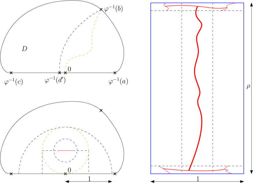
Figure 4. (Left-top) Level lines for $h_{\left(\Omega,a,b,c,d\right)}^{\text{pb}}$ (dashed orange) and the harmonic part $h_{{}^{\prime}}$ (dashed black), endpoint of latter being $\varphi^{-1}(d^{\prime})$. (Left-bottom) Concentric circles around $i/2$ (dashed), and the line $L$ (solid red). (Right) Proof of the upper bound in Corollary 1.4 by positive correlation of crossing events.

∎

6.2. $\varkappa_{m}\to 1$ as $m\to\infty$

We now treat the case where the mass tends to infinity. This is crucial in our analysis of the characteristic length (1.2): sending $m\to\infty$ is equivalent to taking larger and larger rectangles.

Proposition 6.3.

As $m\to\infty$, $\varkappa_{m}\to 1$.

Proof.

For conciseness, we use a compactness argument: similar ideas to Proposition 6.1 may be used to derive more quantitative bounds. Note that, on any compact subset of $\Omega$, $\left\{h_{\left(\Omega,a,b,c,d\right)}\right\}_{m\geq 0}$ is $C^{1}$ bounded by Proposition 3.9; therefore, as in Remark 4.7, by diagonalising we may assume that $h_{\left(\Omega,a,b,c,d\right)}\xrightarrow{m\to\infty}g$. But then Proposition 6.1 in fact implies that $g$ must be a constant. Given that $h_{\left(\Omega,a,b,c,d\right)}$ is bounded below by its harmonic part which is continuous up to $(bc)$ where the boundary value is $1$, the constant must be $g=1$.

Suppose, along some subsequence of $m\to\infty$, $\sup\varkappa_{m}\leq 1-\epsilon<1$. As before, take a pullback domain $D\subset\mathbb{H}$ with $\varphi^{-1}\left(d\right)=0$ and $\left[0,1\right]\subset\left(\varphi^{-1}(c)\varphi^{-1}(a)\right)$. Take small enough $\rho=\rho(\epsilon)>0$ so that on the rectangle $R(\rho):=\left(0,1\right)+\left(0,\rho i\right)\subset D$, the harmonic function $h_{1}$ with boundary values

$$\begin{cases}h_{1}=1-\frac{\epsilon}{2}&\text{on }(\rho i,1+\rho i);\\ h_{1}=0&\text{on }\left(0,\rho i\right)\cup\left(1,1+\rho i\right);\\ h_{1}=\varkappa_{m}&\text{on }\left(0,1\right);\end{cases}$$

has positive inner normal derivatives near $\frac{1}{2}$. Then by taking large enough $m=m(\rho)$ so that $\min_{(\rho i,1+\rho i)}h_{\left(\Omega,a,b,c,d\right)}^{\text{pb}}>1-\frac{\epsilon}{2}$, the superharmonic function $h_{\left(\Omega,a,b,c,d\right)}^{\text{pb}}$ is bounded below by $h_{1}$ and thus $h_{\left(\Omega,a,b,c,d\right)}^{\text{pb}}$ have values strictly greater than $\varkappa_{m}$ near $\frac{1}{2}$. This contradicts $(rh)_{h}^{\text{pb}}$ on $\left(\varphi^{-1}(d)\varphi^{-1}(a)\right)$. ∎

The above proposition directly implies Corollary 1.4 for the specific case of 4-point Dobrushin boundary condition. Specifically, take the rectangle $\Omega:=R(\rho)$ where 4 marked boundary corners are taken at the 4 corners of $R(\rho)$. Then, given $\epsilon$, one may find $m$ large enough such that $\mathrm{p}_{m}\geq 1-\frac{\epsilon}{2}$ by Proposition 6.3. If the upper bound doesn’t hold, we may extract a sequence $\delta_{j}\to 0,q_{j}\delta_{j}^{-1}\to\infty$; in fact by monotonicity (in $q$) we may instead assume $q_{j}\delta_{j}^{-1}\to m$, along which $\mathbb{P}\left[\stackrel{{\scriptstyle\leftrightarrow}}{{R(\rho)^{\delta}}}\right]<1-\epsilon$ and thus is a contradiction to the $\mathrm{p}_{m}$ estimate. Therefore we have the following:

Corollary 6.4.

The upper bound of (1.2) is correct for the 4-point Dobrushin boundary condition.

With the help of the RSW-type estimates (Theorem 1.3) and the FKG inequality, we now extend Corollary 6.4 to general boundary conditions.

Proof of the upper bound in Corollary 1.4.

By monotonicity (with respect to the boundary condition) and arguments as in above, for the upper bound it suffices to show that there is some large $m=m(\epsilon)$ such that for small $\delta<\delta_{0}(m)$ we have $\mathbb{P}\left[\stackrel{{\scriptstyle\leftrightarrow}}{{R(\rho)^{\delta}}}\right]\geq 1-\frac{\epsilon}{2}$ with the dual-wired boundary condition. We show this by intersecting multiple (but a finite number of) crossing events (positively correlated due to FKG inequality), each of which, conditioning on predecessors, has a probability which can be made arbitrarily close to $1$.

Specifically, consider the following events, where we drop the $\delta$ superscript for conciseness (see Figure 4R):

1. For $0<\alpha\ll\rho$ and $j=0,1,2$, the rectangles $(\frac{j}{3},\frac{j+1}{3})+(0,\alpha i)$ in the bottom and $(\frac{j}{3},\frac{j+1}{3})+(i-\alpha i,i)$ on top are crossed vertically;

2. The middles of the top/bottom three $(\frac{1}{3},\frac{2}{3})+(0,\alpha i)$ and $(\frac{1}{3},\frac{2}{3})+(i-\alpha i,i)$ are horizontally crossed;

3. The middle third $(\frac{1}{3},\frac{2}{3})+(0,\rho i)$ of $R(\rho)$ is vertically crossed.

The probability of (1) may be made arbitrarily close to $1$ by setting small enough aspect ratio $\alpha=\alpha(\epsilon)$, by the RSW-type estimate at criticality and then monotonicity in $q$. Conditionally on (1), the probability of (2) may be made arbitrarily close to $1$ by setting large enough $m=m_{1}(\alpha,\epsilon)$ and small enough $\delta<\delta_{0}(m_{1})$, from Proposition 6.3 and comparing with the 4-point Dobrushin boundary condition on the rectangles $(0,1)+(0,\alpha i)$ and $\left(0,1\right)+\left(i-\alpha i,i\right)$. Conditionally on (1) and (2), the probability of (3) may be made arbitrarily close to $1$ by setting large enough $m=m_{2}(m_{1},\alpha,\epsilon)>m_{1}(\alpha,\epsilon)$ and small enough $\delta<\delta_{0}(m_{2})$, again from Proposition 6.3 and comparison with the 4-point Dobrushin boundary condition. ∎

Appendix A Complex Analytic Computations

A.1. Massive S-holomorphicity

In this section, we study the main discrete relations which serve as the counterpart to holomorphicity in the continuum: the (massive) s-holomorphicity. Here we supply the calculations needed to verify the consequences of massive s-holomorphicity: namely the properties of the square integral and that s-holomorphicity is indeed a discretisation of the continuous equation (3.2).

A.1.1. S-holomorphicity on Half-Rhombi

Recall that our discrete domains are composed of rhombi and boundary half-rhombi; the half-rhombi (both in the interior and on the boundary) provide a convenient setting on which s-holomorphicity may be rephrased as intergrability conditions. Consider the dual half-rhombus $T=\left\langle uww_{z}\right\rangle$ around which an s-holomorphic function $F$ may be evaluated at $\xi^{z}:=\left\langle uw\right\rangle$, $\xi_{z}:=\left\langle uw_{z}\right\rangle$, and $z=\left\langle ww_{z}\right\rangle\in\lozenge^{*}$ (see Figure 5). We will be motivated by ’contour integrals’ around $T$: (weighted) sums of function values on $\xi^{z},z,\xi_{z}$ with direction factors $\nu(\xi^{z}),\nu_{T}(z):=\frac{w_{z}-w}{\left|w_{z}-w\right|},-\nu(\xi_{z})$.

Denote the angle surplus $\theta_{z}^{\dagger}=\hat{\theta}_{z}-\bar{\theta}_{z}$. The s-holomorphic projection relations (2.2) are

$$F(z)-ie^{i\theta_{z}^{\dagger}}\nu^{-1}(\xi)\overline{F(z)} =2e^{i\frac{\theta_{z}^{\dagger}}{2}}F(\xi^{z});$$

$$F(z)-ie^{-i\theta_{z}^{\dagger}}\nu^{-1}(\xi_{z})\overline{F(z)} =2e^{-i\frac{\theta_{z}^{\dagger}}{2}}F(\xi_{z}).$$

Immediately we have the ’contour integral’ of $F$: (using $e^{-i\frac{\theta_{z}^{\dagger}}{2}}\nu(\xi^{z})-e^{i\frac{\theta_{z}^{\dagger}}{2}}\nu(\xi_{z})=-2\sin\frac{\hat{\theta}_{z}+\bar{\theta}_{z}}{2}\nu_{T}(z)$)

(A.1) $$F(\xi^{z})\nu(\xi^{z})+\sin\frac{\hat{\theta}_{z}+\bar{\theta}_{z}}{2}F(z)\nu_{T}(z)-F(\xi_{z})\nu(\xi_{z})=\sin\frac{\theta_{z}^{\dagger}}{2}\overline{F(z)}.$$

Alternatively, we may eliminate $\overline{F(z)}$: (using $e^{-i\theta_{z}^{\dagger}}\nu(\xi^{z})-e^{i\theta_{z}^{\dagger}}\nu(\xi_{z})=-2\sin\hat{\theta}_{z}\nu_{T}(z)$),

(A.2) $$\sin\hat{\theta}_{z}F(z)\nu_{T}(z)=e^{i\frac{\theta_{z}^{\dagger}}{2}}\nu(\xi_{z})F(\xi_{z})-e^{-i\frac{\theta_{z}^{\dagger}}{2}}\nu(\xi^{z})F(\xi^{z}),$$

which, once squared, gives (recall $\nu(\xi_{z})=-ie^{i\bar{\theta}_{z}}\nu_{T}(z)$, $\nu(\xi^{z})=-ie^{-i\bar{\theta}_{z}}\nu_{T}(z)$)

$$\left(\sin\hat{\theta}_{z}F(z)\nu_{T}(z)\right)^{2}$$

$$= e^{i\theta_{z}^{\dagger}}\nu(\xi_{z})^{2}F(\xi_{z})^{2}+e^{-i\theta_{z}^{\dagger}}\nu(\xi^{z})^{2}F(\xi^{z})^{2}-2\nu(\xi)\nu(\xi_{z})F(\xi_{z})F(\xi)$$

$$= -\nu_{T}(z)\left(ie^{i\hat{\theta}_{z}}F(\xi_{z})^{2}\nu(\xi_{z})+ie^{-i\hat{\theta}_{z}}F(\xi^{z})^{2}\nu(\xi^{z})-2\nu_{T}(z)F(\xi_{z})F(\xi)\right).$$

Dividing by $\nu_{T}(z)$ and rearranging, we get a ’contour integral’ of $F^{2}$ (noting phases of $F(\xi^{z}),F(\xi_{z})$)

$$F(\xi^{z})^{2}\nu(\xi^{z})+\sin\hat{\theta}_{z}F(z)^{2}\nu_{T}(z)-F(\xi_{z})^{2}\nu(\xi_{z})$$

$$= \frac{2\nu_{T}(z)F(\xi_{z})F(\xi^{z})-i\cos\hat{\theta}_{z}F(\xi_{z})^{2}\nu(\xi_{z})-i\cos\hat{\theta}_{z}F(\xi^{z})^{2}\nu(\xi^{z})}{\sin\hat{\theta}_{z}}$$

$$= \frac{2\nu_{T}(z)F(\xi_{z})F(\xi^{z})-\cos\hat{\theta}_{z}\left(\left|F(\xi_{z})\right|^{2}+\left|F(\xi^{z})\right|^{2}\right)}{\sin\hat{\theta}_{z}}\in\mathbb{R}.$$

Noting the phase of $F(\xi^{z})$ and $F(\xi_{z})$, we may re-write the above in real and imaginary parts, both of which are useful. First, since both values are projections of $F(z)$, we may naturally compute $d:=\arg F(\xi_{z})-\arg F(\xi^{z})=-\bar{\theta}_{z},\pi-\bar{\theta}_{z}$. Define $\left[\operatorname{da}_{u}F\right](z)=\cos\left(d+\bar{\theta}_{z}\right)\in\left\{\pm 1\right\}$, chosen to be $-1$ if either value of $F$ is zero. Then we have

(A.3) $$\operatorname{Re}\left[\sin\hat{\theta}_{z}F(z)^{2}\nu_{T}(z)\right] =\frac{2\left[\operatorname{da}_{u}F\right](z)\left|F(\xi_{z})\right|\left|F(\xi^{z})\right|-\cos\hat{\theta}_{z}\left(\left|F(\xi_{z})\right|^{2}+\left|F(\xi^{z})\right|^{2}\right)}{\sin\hat{\theta}_{z}}$$

(A.4) $$\operatorname{Im}\left[\sin\hat{\theta}_{z}F(z)^{2}\nu_{T}(z)\right] =\operatorname{Im}\left[-F(\xi^{z})^{2}\nu(\xi^{z})+F(\xi_{z})^{2}\nu(\xi_{z})\right]=\left|F(\xi^{z})\right|^{2}-\left|F(\xi_{z})\right|^{2}.$$

Remark A.1.

To have a complete treatment, we need to do the analogue on a primal half-rhombus $T^{{}^{\prime}}:=\left\langle uwu_{z}\right\rangle$. Thanks to duality, $iF$ could be said to be s-holomorphic on the same rhombus with the primal and dual vertices interchanged, as long as we make the corresponding adjustments in (2.2): $\bar{\theta}_{z}\to\frac{\pi}{2}-\bar{\theta}_{z}$, $\hat{\theta}_{z}\to\frac{\pi}{2}-\hat{\theta}_{z}$. Carefully applying the above, we have ($\xi_{z}^{\prime}:=\left\langle u_{z}w\right\rangle,\nu_{T^{\prime}}(z):=i\nu_{T}(z)$)

$$F(\xi^{z})\nu(\xi^{z})+\cos\frac{\hat{\theta}_{z}+\bar{\theta}_{z}}{2}F(z)\nu_{T^{\prime}}(z)-F(\xi_{z}^{\prime})\nu(\xi_{z}^{\prime})= \sin\frac{\theta_{z}^{\dagger}}{2}\overline{F(z)},$$

$$-\text{Re}\sin\hat{\theta}_{z}\nu_{T^{\prime}}(z)F(z)^{2}+\left|F(z)\right|^{2}=\left|F(\xi^{z})\right|^{2} +\left|F(\xi_{z}^{\prime})\right|^{2},$$

and

$$\operatorname{Re}\left[\cos\hat{\theta}_{z}F(z)^{2}\nu_{T^{\prime}}(z)\right] =\frac{2\left[\operatorname{da}_{w}F\right](z)\left|F(\xi^{\prime}_{z})\right|\left|F(\xi^{z})\right|-\sin\hat{\theta}_{z}\left(\left|F(\xi^{\prime}_{z})\right|^{2}+\left|F(\xi^{z})\right|^{2}\right)}{\cos\hat{\theta}_{z}},$$

$$\operatorname{Im}\left[\cos\hat{\theta}_{z}F(z)^{2}\nu_{T^{\prime}}(z)\right] =\operatorname{Im}\left[-F(\xi^{z})^{2}\nu(\xi^{z})+F(\xi_{z}^{\prime})^{2}\nu(\xi_{z}^{\prime})\right]=\left|F(\xi^{z})\right|^{2}-\left|F(\xi_{z}^{\prime})\right|^{2}.$$

where $\left[\operatorname{da}_{w}F\right](z)$ is defined similarly using the argument turning from $\xi^{\prime}_{z}$ to $\xi^{z}$.

A.1.2. $\bar{\partial}$ Calculations

Given the computation on half-rhombi given in the previous section, we may combine them to calculate contour integrals involving only values on edges $z\in\lozenge$, which scale to ’physical’ contour integrals in the continuum. First, we will give exact calculations for some auxiliary operators $\bar{\partial}_{1,2,3}^{\delta}$ which we will introduce now; the terms arising from the difference $\bar{\partial}^{\delta}-\bar{\partial}_{1,2,3}^{\delta}$ will be estimated to be small for our purposes. Define (recall $2\mu^{\delta}(u)$ is the total area of the half-rhombi $T$ around $u$)

$$\bar{\partial}_{1}^{\delta}F_{0}(u) :=\frac{1}{2i\mu_{\Gamma}^{\delta}(u)}\sum_{z\sim u}\frac{\sin\frac{\hat{\theta}_{z}+\bar{\theta}_{z}}{2}}{\sin\bar{\theta}_{z}}(w_{z}-w)F_{0}(z),$$

$$\bar{\partial}_{2}^{\delta}F_{0}(u) :=\frac{1}{2i\mu_{\Gamma}^{\delta}(u)}\sum_{z\sim u}\frac{\sin^{2}\hat{\theta}_{z}}{\sin^{2}\bar{\theta}_{z}}(w_{z}-w)F_{0}(z),$$

$$\bar{\partial}_{3}^{\delta}F_{0}(u) :=\frac{1}{2i\mu_{\Gamma}^{\delta}(u)}\sum_{z\sim u}\frac{\cos\hat{\theta}_{z}}{\cos\bar{\theta}_{z}}(w_{z}-w)F_{0}(z),$$

on $u\in\Gamma$ for functions $F_{0}$ defined on $\lozenge$. Both degenerate to $\bar{\partial}^{\delta}$ when $k=0$. Then, summing (A.1), (A.3) around $u$, it remains to study the exact expressions

$$\bar{\partial}_{1}^{\delta}F(u)=\frac{1}{2i\mu_{\Gamma}^{\delta}(u)}\sum_{z\sim u}2\delta\sin\frac{\theta_{z}^{\dagger}}{2}\overline{F(z)},$$

and

(A.5) $$\bar{\partial}_{2}^{\delta}F^{2}(u)=\frac{2\delta}{2i\mu_{\Gamma}^{\delta}(u)}\sum_{z\sim u}\frac{2\nu_{T}(z)F(\xi_{z})F(\xi^{z})-\cos\hat{\theta}_{z}\left(\left|F(\xi_{z})\right|^{2}+\left|F(\xi^{z})\right|^{2}\right)}{\sin\bar{\theta}_{z}}.$$

We start by showing that the massive s-holomorphic functions indeed do converge to massive holomorphic functions.

Lemma A.2.

If a family $\left\{F^{\delta}\right\}_{\delta>0}$ of s-holomorphic functions on $\Omega_{\delta}$ converges locally uniformly to a locally Lipschitz continuous function $f$ on $\Omega$, then $f$ is massive holomorphic.

Proof.

Because of Remark 3.1, it suffices to show that for any ball $\overline{B_{r}}\subset\Omega$, we have (3.2) in the areolar derivative sense:

(A.6) $$\oint_{\partial B_{r}}fdz=2i\iint_{B_{r}}-mi\bar{f}d^{2}z.$$

Find a simple path $\partial B_{r}^{\delta}$ of dual edges converging in Hausdorff distance to $\partial B_{r}$ as $\delta\downarrow 0$ and consider the discrete domain $B_{r}^{\delta}$ within (constructed, e.g., as the boundary of a discrete ball thanks to bounded angle property). Then by definition (4.2) and telescoping (as in the proof of discrete divergence theorem),

$$\sum_{z\in\partial B_{r}^{\delta}}\frac{\sin\frac{\hat{\theta}_{z}+\bar{\theta}_{z}}{2}}{\sin\bar{\theta}_{z}}(w_{z}-w)F(z) =\sum_{u\in\Gamma\cap B_{r}^{\delta}}2i\mu_{\Gamma}^{\delta}(u)\bar{\partial}_{1}^{\delta}F(u)$$

$$=\sum_{z^{\prime}\in\lozenge\cap B_{r}^{\delta}}4\delta\sin\frac{\theta_{z^{\prime}}^{\dagger}}{2}\overline{F(z^{\prime})},$$

where the factor of $2$ comes from the fact that any $z^{\prime}$ is counted twice from two incident $u\in\Gamma$. As $\delta\downarrow 0$, it’s clear that the sums on LHS and RHS respectively converge to those of (A.6). ∎

Now we move on to a more involved calculation. We need to study $\bar{\partial}_{2}^{\delta}F^{2}(u)$ in (A.5),and $\bar{\partial}_{3}^{\delta}F^{2}(u)$, which corresponds exactly to the Laplacian with behaviour stated in (4.6). Sum of the same type was studied in [ChSm12], but the abstract angles $\hat{\theta}_{z}$ here do not sum to $\pi$ around a vertex $u$, giving rise to an $L^{2}$ -term of $F$.

Proposition A.3.

There are real quantities $A\left(\left\{\bar{\theta}_{z}\right\},m\right)$, $B(\left\{F(\xi_{z})\right\}_{z\sim u})\geq 0$ such that

(A.7) $$2i\delta^{-1}\mu_{\Gamma}^{\delta}(u)\bar{\partial}_{2}^{\delta}F^{2}(u) =\sum_{z\sim u}\frac{2\left(\cos\bar{\theta}_{z}-\cos\hat{\theta}_{z}\right)}{\sin\bar{\theta}_{z}}\left(\left|F(\xi_{z})\right|^{2}+\left|F(\xi^{z})\right|^{2}\right)-B(\left\{F(\xi_{z})\right\}_{z\sim u}),$$

(A.8) $$2i\delta^{-1}\mu_{\Gamma}^{\delta}(u)\bar{\partial}_{3}^{\delta}F^{2}(u) =\sum_{z\sim u}A\left(\bar{\theta}_{z},\hat{\theta}_{z}\right)\left(\left|F(\xi_{z})\right|^{2}+\left|F(\xi^{z})\right|^{2}\right)-B(\left\{F(\xi_{z})\right\}_{z\sim u}),$$

where $A\left(\left\{\bar{\theta}_{z}\right\},m\right)\apprle m\delta\sin 2\bar{\theta}_{z}$ with asymptotic not dependent on the uniform bound $\eta$.

Proof.

As in the proof of Proposition 2.2, define $x_{\xi_{z}}:=\left(i\nu(\xi_{z})\right)^{1/2}F(\xi_{z})$, where $\left(i\nu\left(\xi_{z}\right)\right)^{1/2}$ varies continuously as we turn around $u$ once (i.e. the ’cut’ is placed between the last and the first corners). The proof of [ChSm12, Proposition 3.6] proves that the quadratic form $Q$ (which we take to be $\frac{1}{2}B(\left\{F(\xi_{z})\right\}_{z\sim u})$)

$$\sum_{z\sim u}\frac{\cos\bar{\theta}_{z}\left(\left|F(\xi_{z})\right|^{2}+\left|F(\xi^{z})\right|^{2}\right)-2\nu_{T}(z)F(\xi_{z})F(\xi^{z})}{\sin\bar{\theta}_{z}}=:Q_{\left\{\overline{\theta}_{z}\right\}_{z\sim u}}^{\deg u}\left(\left\{x_{\xi_{z}}\right\}_{z\sim u}\right)$$

is always nonnegative, no matter what the real numbers $x_{\xi_{z}}$ are. This establishes (A.7).

Now it remains to control $\left(\bar{\partial}_{3}^{\delta}-\bar{\partial}_{2}^{\delta}\right)F^{2}(u)$. But by (1.1)

$$2i\delta^{-1}\mu_{\Gamma}^{\delta}(u)\left(\bar{\partial}_{3}^{\delta}-\bar{\partial}_{2}^{\delta}\right)F^{2}(u) =\delta^{-1}\sum_{z\sim u}\left(\frac{\cos\hat{\theta}_{z}}{\cos\bar{\theta}_{z}}-\frac{\sin^{2}\hat{\theta}_{z}}{\sin^{2}\bar{\theta}_{z}}\right)(w_{z}-w)F^{2}(z)$$

$$=O(m\delta\sin 2\bar{\theta}_{z})\sum_{z\sim u}\left(\left|F(\xi_{z})\right|^{2}+\left|F(\xi^{z})\right|^{2}\right).$$

∎

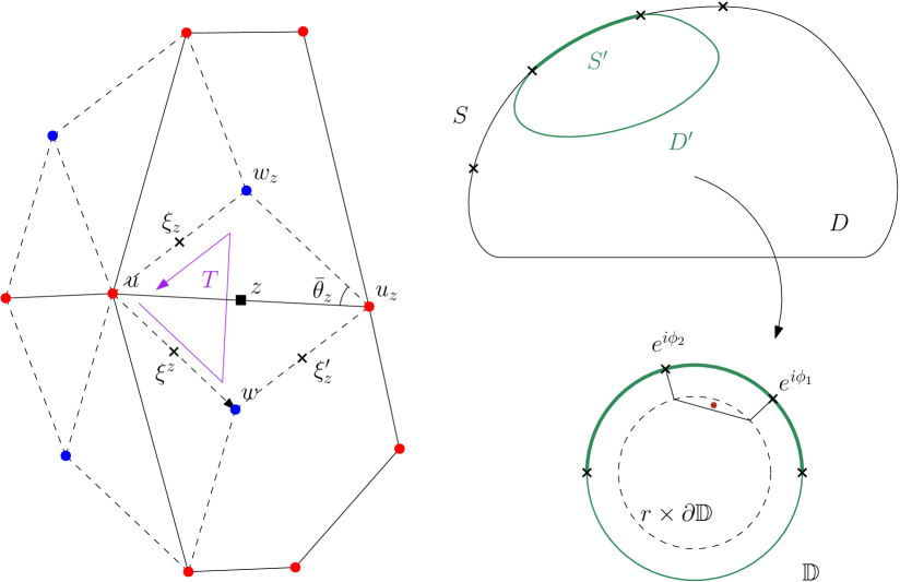
Figure 5. (Left) Local notation given the primal vertex $u$ and an incident edge $z$; dual half-rhombus $T$ and discrete integration contour around $T$. (Right) Setting for the proof of Proposition A.9: note that the crescent-shaped domain (brown bullet) has a fixed shape.

A.2. Massive Cauchy Formulae

In this section, we recall the Cauchy integral formula for the continuum massive holomorphic functions, and construct its discrete counterpart. The discrete version is also a generalisation of its critical counterpart, namely [ChSm12, Lemma A.6].

A.2.1. Continuous Case

Recall that for $l\in\mathbb{N}$ the modified Bessel functions of the second kind $K_{l}(r)$ is the radial solution to the equation $\Delta_{r,\phi}\left[e^{-il\phi}K_{l}(r)\right]=\left[e^{-il\phi}K_{l}(r)\right]$ with the asymptotics $K_{l}(r)\sim\frac{\left(l-1\right)!}{2}\left(\frac{1}{2}r\right)^{-l}$ (while $K_{0}(r)\sim-\ln r$) as $r\downarrow 0$ and $K_{l}(r)\sim\sqrt{\frac{\pi}{2r}}e^{-r}$ as $r\to\infty$. In particular, $\left|K_{l}(r)\right|\leq\operatorname{C}_{l}r^{-l}$.

They can be combined in order to construct massive holomorphic functions with the same asymptotics (e.g. [Par19, (2.16)]), of which we consider the following massive versions of the Cauchy kernel $\frac{1}{z^{\prime}}$. Recalling the radial derivative $\bar{\partial}g=\frac{e^{i\phi}}{2}\left(\partial_{r}+ir^{-1}\partial_{\phi}\right)$, define the massive holomorphic (or rather, meromorphic) functions

$$\zeta_{-1}^{1}\left(z^{\prime}=re^{i\phi}\right) :=2m\left[e^{-i\phi}K_{1}\left(2mr\right)+iK_{0}\left(2mr\right)\right];$$

$$\zeta_{-1}^{i}\left(z^{\prime}=re^{i\phi}\right) :=2m\left[ie^{-i\phi}K_{1}\left(2mr\right)+K_{0}\left(2mr\right)\right],$$

having the asymptotics $\zeta_{-1}^{1}(z^{\prime})\sim\frac{1}{z^{\prime}}$ and $\zeta_{-1}^{i}(z^{\prime})\sim\frac{i}{z^{\prime}}$ as $w\to 0$. Their massive holomorphicity follows straightforwardly from the recurrence relation $K_{l}^{\prime}(r)=-K_{l\pm 1}(r)\pm lr^{-1}K_{l}(r)$. Recursively, the following estimate holds as well:

Lemma A.4.

The functions $\zeta_{-1}^{1},\zeta_{-1}^{i}$ are smooth away from $w=0$, and has asymptotics

$$\left|\partial^{(l)}\text{$\zeta_{-1}^{1}$}(z^{\prime})\right|,\left|\partial^{(l)}\text{$\zeta_{-1}^{i}$}(z^{\prime})\right|\leq\operatorname{C}_{l}\left|z^{\prime}\right|^{-l-1},$$

where $\partial^{(l)}$ refers to any $l$-th derivative.

Recall that smoothness is a consequence (Corollary 3.8) of the following proposition, so we only assume below that $f$ is locally Lipschitz, and use Green’s theorem as described in Remark 3.1.

Proposition A.5 (Continuum Cauchy Integral Formula [Ber56, Section 6]).

For any massive holomorphic function $f$ defined in a neighbourhood of $w$, we have

(A.9) $$f(z)=\frac{1}{2\pi}\left[\operatorname{Im}\oint_{\omega}f(z^{\prime})\zeta_{-1}^{1}(z-z^{\prime})dz^{\prime}-i\operatorname{Im}\oint_{\omega}f(z^{\prime})\zeta_{-1}^{i}(z-z^{\prime})dz^{\prime}\right],$$

for any simple integration contour $\omega$ surrounding $w$ in the domain of definition.

Proof.

Recall that the imaginary part of the integral of the square of a massive holomorphic function is well-defined. Given bilinearity, by polarisation the imaginary part of the integral of a product of two massive holomorphic functions is well-defined as well. Therefore, the above integrals may be computed around any contour around $z^{\prime}$, which we take as a small circle $\partial B_{r}(z^{\prime})$ around $z^{\prime}$. Given uniform continuity of $f$ and the asymptotics for $\zeta_{-1}^{1,i}$, we clearly have $\operatorname{Im}\oint_{\partial B_{r}(z)}f(z^{\prime})\zeta_{-1}^{1}(z-z^{\prime})dz^{\prime}\to 2\pi\operatorname{Re}f(z)$ and $\operatorname{Im}\oint_{\partial B_{r}(z)}f(z^{\prime})\zeta_{-1}^{i}(z-z^{\prime})dz^{\prime}\to-2\pi\operatorname{Im}f(z)$ as $r\to 0$. ∎

A.2.2. Discrete Case

The discrete contour integral for a product of two (massive) s-holomorphic functions should be understood as polarisation of the discrete square integral in Lemma 2.5:

$$\operatorname{Im}\int^{\delta}2FZdz:=\operatorname{Im}\int^{\delta}(F+Z)^{2}dz-\operatorname{Im}\int^{\delta}F^{2}dz-\operatorname{Im}\int^{\delta}Z^{2}dz,$$

defined on (a connected subset of) $\Gamma\cup\Gamma^{*}$. We also define $\operatorname{Im}\oint^{\delta}$ along a closed loop of primal and/or dual vertices on $\Gamma\cup\Gamma^{*}$, which is clearly locally well-defined as long as both functions are s-holomorphic but might have a monodromy around a ’singularity’, as in below.

We need discrete s-holomorphic functions corresponding to the continuous kernels $\zeta_{-1}^{1,i}$. For each $z\in\lozenge$ consider discrete functions $Z_{-1}^{1,i}(z,\cdot)$ having following properties:

• $Z_{-1}^{1,i}(z,\cdot)$ is defined and massive s-holomorphic on $\lozenge\cup\Upsilon\setminus\left\{z\right\}$;

• Write $Z^{\tau}=Z_{-1}^{\tau}(z,\cdot)$. If we were to define $Z^{\tau}(z)$ as the value satisfying (2.2) for a pair of adjacent corners (i.e. using the formula (A.2)), we may define two values $Z_{z},Z_{z}^{\prime}$ coming respectively from the pairs $\xi_{z},\xi^{z}$ and $\xi_{z}^{\prime},\left(\xi^{z}\right)^{\prime}$ (see Figure 5L). Then we have

  (A.10) $$\sin\hat{\theta}_{z}(Z_{z}-Z_{z}^{\prime})\nu_{T}(z)=i\tau\cdot\pi\delta^{-1}.$$

Proposition A.6.

For such discrete kernels $Z_{-1}^{\tau}$ and any massive s-holomorphic function $F$ defined in a neighbourhood of $z\in\lozenge$, we have

$$F(z)=\frac{1}{2\pi}\left[\operatorname{Im}\oint_{\omega^{\delta}}^{\delta}F(z^{\prime})Z_{-1}^{1}(z,z^{\prime})dz^{\prime}-i\operatorname{Im}\oint_{\omega^{\delta}}^{\delta}F(z^{\prime})Z_{-1}^{i}(z,z^{\prime})dz^{\prime}\right],$$

for any simple discrete contour $\omega^{\delta}$ surrounding $z^{\prime}$.

Proof.

Since the contour for the integral $\operatorname{Im}\int^{\delta}$ may be deformed without crossing singularities, we may take $\omega^{\delta}$ as the smallest contour $\omega_{z}=\xi_{z}\sim\xi^{z}\sim\xi_{z}^{\prime}\sim\left(\xi^{z}\right)^{\prime}$ around $z$.

Then inspecting (2.4) and the condition (A.10), we see (by splitting $\omega_{z}$ into two half-rhombi)

$$\operatorname{Im}\oint_{\omega^{\delta}}^{\delta}F(z^{\prime})Z_{-1}^{\tau}(z,z^{\prime})dz=2\delta\times\operatorname{Im}\left[\sin\hat{\theta}_{z}(Z_{z}-Z_{z}^{\prime})F(z)\nu_{T}(z)\right]=2\pi\operatorname{Im}\left[i\tau F(z)\right],$$

which yields the result. ∎

In fact, construction for such discrete kernels is done in [CIM21] using massive discrete exponentials (see also [BdTR17]). We explain how to apply their construction in our setup.

Proposition A.7 ([CIM21, Section 5]).

The kernels $Z_{-1}^{1,i}(z,z^{\prime})$ may be constructed using explicit contour integrals (involving the angles of a path from $z$ to $z^{\prime}$), and have the uniform asymptotic

(A.11) $$Z_{-1}^{1,i}(z,z^{\prime})=\zeta_{-1}^{1,i}(z-z^{\prime})+O\left(\delta\right),$$

and thus

$$Z_{-1}^{1,i}(z,z^{\prime})-Z_{-1}^{1,i}(z^{\delta},z^{\prime})=O(\delta),$$

for $z\sim z^{\delta}\in\lozenge$, where $m\asymp q\delta^{-1},|z-z^{\prime}|$ are uniformly bounded away from $0$ and $\infty$.

In fact, for $z\neq z^{\prime}$,

(A.12) $$Z_{-1}^{1,i}(z,z^{\prime})\apprle\frac{1}{|z-z^{\prime}|}.$$

These estimates hold for small $q$, and only depend on the respective uniform conditions and the uniform angle bound $\eta$.

Proof.

Let us summarise the consequences of [CIM21, Proposition 5.8]: for corners $a\neq c$, [CIM21, (5.15)] constructs a real function $\mathrm{G}_{(a)}(c)$ which branches (switches sign) around every vertex and face and satisfies the three-point propagation equation in $c$. Then as in the proof of Proposition 2.2, we may define non-branching function $\Xi(a,c):=\left(i\nu(c)\right)^{-1/2}\mathrm{G}_{(a)}(c)$ which may be extended to a massive s-holomorphic function $\Xi(a,\cdot)$. At $a$, the value of $\Xi(a,\cdot)$ respecting the s-holomorphicity condition (2.2) is $\left(i\nu(a)\right)^{-1/2}$ with the edge to the left of $a$ facing the direction of $\nu(a)$, while it is $-\left(i\nu(a)\right)^{-1/2}$ to the right.

Now, given $z$ as in Figure 5L, we will set $\Xi(\xi_{z},\xi_{z}):=\left(i\nu(\xi_{z})\right)^{-1/2}$ and $\Xi(\xi_{z}^{\prime},\xi_{z}^{\prime}):=\left(i\nu(\xi_{z}^{\prime})\right)^{-1/2}:=-i\left(i\nu(\xi_{z})\right)^{-1/2}$, i.e. so that they are s-holomorphic away from $z$. We would like to real-linear combine these two functions so that we have (A.10). For $Z=\Xi(\xi_{z},\cdot)$, the difference $Z_{z}-Z_{z}^{\prime}$ would have been zero had $\Xi(\xi_{z},\xi_{z})$ been defined as $-\left(i\nu(\xi_{z})\right)^{-1/2}$ (so that it would be s-holomorphic with respect to $z$): therefore, $\sin\hat{\theta}_{z}(Z_{z}-Z_{z}^{\prime})\nu_{T}(z)=-2ie^{i\frac{\theta_{z}^{\dagger}}{2}}\left(i\nu(\xi_{z})\right)^{1/2}$, which is precisely the contribution in (A.2) coming from switching $-\left(i\nu(\xi_{z})\right)^{-1/2}$ to $\left(i\nu(\xi_{z})\right)^{-1/2}$. For $Z=\Xi(\xi_{z}^{\prime},\cdot)$, similar computation gives $\sin\hat{\theta}_{z}(Z_{z}-Z_{z}^{\prime})\nu_{T}(z)=2ie^{i\frac{\theta_{z}^{\dagger}}{2}}\left(i\nu(\xi_{z}^{\prime})\right)^{1/2}=-2ie^{i\frac{\theta_{z}^{\dagger}}{2}}\left(i\nu(\xi_{z})\right)^{1/2}\cdot i$.

Therefore, we may set (recalling the notation $\left(i\nu(\hat{\xi}_{z})\right)^{1/2}:={e^{i\frac{\theta_{z}^{\dagger}}{2}}\left(i\nu(\xi_{z})\right)^{1/2}}$ from Proposition 2.2)

$$Z_{-1}^{1}(z,z^{\prime}) :=\frac{\pi}{2\delta}\left(\operatorname{Im}{\left(i\nu(\hat{\xi}_{z})\right)^{1/2}}\Xi(\xi_{z},z^{\prime})+\operatorname{Re}{\left(i\nu(\hat{\xi}_{z})\right)^{1/2}}\Xi(\xi_{z}^{\prime},z^{\prime})\right)$$

$$Z_{-1}^{i}(z,z^{\prime}) :=\frac{\pi}{2\delta}\left(\operatorname{Im}{\left(i\nu(\hat{\xi}_{z})\right)^{1/2}}\Xi(\xi_{z}^{\prime},z^{\prime})-\operatorname{Re}{\left(i\nu(\hat{\xi}_{z})\right)^{1/2}}\Xi(\xi_{z},z^{\prime})\right).$$

Then (A.11) follows straightforwardly from [CIM21, (5.30), (5.25)] (cf. also [CIM21, Theorem 3.16]).

For the cruder uniform estimate (A.12), we essentially give a cruder version of the proof of [CIM21, (5.30)]: we will use their conventions, note especially the conversion $\check{x}=\frac{2K}{\pi}x$ [CIM21, (5.1)] between ’elliptic’ and physical angles. For the main definition [CIM21, (5.15)] of the discrete exponential, the path $a\sim w_{0}\sim\cdots\sim w_{n}\sim c$, $w_{j}\in\Lambda$ is chosen, such that the arguments of successive segments $\phi_{w_{0}a}:=\arg(w_{0}-a),\ldots$ are all contained in a segment of length $\pi-2\eta$, whose midpoint is denoted $\phi^{\Lambda}_{ca}$. After the variable shift $\check{\nu}=\check{\mu}-2iK^{\prime}$, the integral in $\check{\nu}$ is computed on the broken line passing through the points $\check{\phi}^{\Lambda}_{ca}-2iK^{\prime},\check{\phi}^{\Lambda}_{ca}-iK^{\prime},\check{\phi}_{ca}-iK^{\prime},\check{\phi}_{ca}+iK^{\prime},\check{\phi}^{\Lambda}_{ca}+iK^{\prime},\check{\phi}^{\Lambda}_{ca}+2iK^{\prime}$. The real parameter $y\in[-1,1]$ is introduced so that $\operatorname{Im}\check{\nu}=2K^{\prime}y$ and $\operatorname{Im}\nu=-{y}\log q$.

• When $\left|\operatorname{Im}\check{\nu}\right|\leq iK^{\prime}$, the estimate [CIM21, Remark 5.10] corresponding to the first identity of [CIM21, (5.24)] (which is uniform in $|c-a|$) implies that the integrand is bounded by a constant multiple of

  $$k^{2}(k^{\prime})^{-\frac{1}{2}}\left|\cos\left(\frac{1}{2}(\nu-\phi_{w_{0}a})\right)\cos\left(\frac{1}{2}(\nu-\phi_{cw_{n}})\right)\exp\left[-2m|c-a|\cos\left(\nu-\phi_{ca}\right)\right]\right|$$

  $$\apprle qq^{-|y|}\exp\left[-2m(\sin\eta)|c-a|\cosh(\operatorname{Im}\nu)\right]\leq q^{1-|y|}\exp\left[-m(\sin\eta)|c-a|q^{-|y|}\right],$$

  since $\operatorname{Re}\check{\nu}$ is between $\check{\phi}_{ca}$ and $\check{\phi}^{\Lambda}_{ca}$, such that $\left|\operatorname{Re}\nu-\phi_{ca}\right|\leq\frac{\pi}{2}-\eta$. So, for the three integration line segments in this region:

  • For the middle vertical segment $\left[\check{\phi}_{ca}-iK^{\prime},\check{\phi}_{ca}+iK\right]$, we multiply by $(-\log q)i\cdot dy$ and integrate over $y=[-1,1]$, which can be done explicitly and yield an $O(\frac{q}{m(\sin\eta)|c-a|})\apprle\frac{\delta}{|c-a|}$ estimate, as desired.

  • For the horizontal segments between $\check{\phi}^{\Lambda}_{ca}\pm iK^{\prime}$ and $\check{\phi}_{ca}\pm iK$ (which is of $O(1)$ length), simply bound by the the maximum over $q^{-|y|}$, which is $\frac{e^{-1}q}{m(\sin\eta)|c-a|}$.

• For the vertical line segments $\left[\check{\phi}^{\Lambda}_{ca}\pm iK^{\prime},\check{\phi}^{\Lambda}_{ca}\pm 2iK^{\prime}\right]$, we give a similar integral bound, relying on the fact that if $\operatorname{Re}\check{\nu}=\check{\phi}^{\Lambda}_{ca}$, any $z:=\frac{1}{2}(\nu-\phi)$ coming from the integrand has $\left|\operatorname{Re}2z\right|\leq\frac{\pi}{2}-\eta$, so $2q\cos(2z)\in\mathbb{D}^{\eta}:=\{\zeta:|\zeta|<1,\arg\zeta\in\left[-\frac{\pi}{2}+\eta,\frac{\pi}{2}-\eta\right]\}$. The integrand to be estimated is the product of (cf. especially [CIM21, Remark 5.10, (5.19)]): $-ik\left(k^{\prime}\right)^{-\frac{1}{4}}\operatorname{cd}\left(\frac{1}{2}(\check{\nu}-\check{\phi}_{w_{0}a})|k\right)$, $-\sqrt{k^{\prime}}\operatorname{nd}\left(\frac{1}{2}(\check{\nu}-\check{\phi}_{w_{j+1}w_{j}})|k\right)$ for $j=0,\ldots,n-1$, and $ik\left(k^{\prime}\right)^{\frac{1}{4}}\operatorname{cd}\left(\frac{1}{2}(\check{\nu}-\check{\phi}_{cw_{n}})|k\right)$, each corresponding to the segments of the path chosen for the discrete exponential.

  From [DLMF, 22.2, 20.2] (cf. [CIM21, (5.22)] and the discussion):

  $$\left|\operatorname{cd}\left(\check{z}|k\right)\right| =\left|\frac{({1+O(q)})(\cos(z)+O(q^{1/2}))}{1+2q\cos(2z)+O(q^{2})}\right|;$$

  $$\left|\sqrt{k^{\prime}}\operatorname{nd}\left(\check{z}|k\right)\right| =\left|\frac{1-2q\cos(2z)+O(q^{2})}{1+2q\cos(2z)+O(q^{2})}\right|.$$

  In $\mathbb{D}^{\eta}$, there is a constant $c(\eta)>0$ such that $\left|\frac{1-\zeta}{1+\zeta}\right|\leq 1-c(\eta)\operatorname{Re}\zeta$. Therefore we have for small $q$:

  $$\left|\operatorname{cd}\left(\check{z}|k\right)\right|\apprle\left|\cos(z)\right|\leq q^{-|y|/2};\log\left|\sqrt{k^{\prime}}\operatorname{nd}\left(\check{z}|k\right)\right|\apprle-\operatorname{Re}\left[2q\cos(2z)\right]+q^{2}\apprle-q^{1-|y|}.$$

  We use the first estimate twice (start and end) and the second $n\asymp\delta^{-1}|a-c|$ times, then integrate with $(-\log q)i\cdot dy$ as above, yielding an $O(\frac{q^{3/2}}{m(\sin\eta)|c-a|})$ estimate for $\mathrm{G}_{(a)}(c)$.

∎

In fact, we could have constructed the same kernels $Z_{-1}^{1,i}(z,z^{\prime})$ starting from any two corners around $z$; although these kernels are not antisymmetric in its variables per se, the two variables may be considered on an equal footing, so there is a relation for the variable $z$ which is equivalent to the s-holomorphicity for $z^{\prime}$: see e.g. [GHP19].

A.3. $W^{1,p}$-factorisation

In this section, we collect deeper Sobolev space theory and carry out detailed analysis near the boundary $\partial D$. Recall the linear (i.e. length) and planar (i.e. area) Hausdorff measures $\mathcal{H}^{1,2}$ on $\mathbb{C}$. We first recall the notion of Lebesgue points of Sobolev functions, and how it may be used to define the trace $\mathcal{H}^{1}$-almost everywhere.

We first recall some general facts, of crucial use in [BBC16].

Lemma A.8.

Let $p\in(1,2)$ and $U$ be a bounded domain whose boundary is locally a graph of a Lipschitz function.

1. Any function $g\in W^{1,p}(U)$ may be strictly defined (i.e. by the limit of integral averages) pointwise at its Lebesgue points, whose complement is a $\mathcal{H}^{1}$-null set.

2. There is a continuous extension operator $W^{1,p}(U)\to W^{1,p}(\mathbb{C})$. The restriction to $\mathcal{H}^{1}$-almost all vertical and horizontal lines of a function in $W^{1,p}(\mathbb{C})$ is absolutely continuous.

3. The trace $\operatorname{tr}_{\partial U}g$ may be obtained as the restriction on $\partial U$ of the strictly defined version of any extension of $g$ to $\mathbb{C}$. More generally, the restriction of $g$ is well-defined $\mathcal{H}^{1}$-almost everywhere.

4. The exponential function maps $W^{1,2}(U)$ into $W^{1,p}(U)$ continuously for any $p\in(1,2)$, and therefore into $L^{q}\left(U\right)$ for any $q\in[1,\infty)$.

5. The trace operator commutes with exponential, and $\operatorname{tr}_{\partial U}e^{g}\in L^{q}\left(\partial U\right)$ for any $q\in[1,\infty)$.

Proof.

The introduction of [BBC16] recalls the standard facts (1), (3) and the first half of (2). The second half of (2) is the so-called ACL characterisation of Sobolev functions, e.g. [EvGa15, Theorem 4.21]. (4) and (5) are proved in [BBC16, Proposition 8.4]. ∎

We are ready to show that the constant boundary condition, which constitutes half of the condition $(rh)_{h}$, is preserved under multiplication by $e^{s}$. Note in the following we assume local boundedness near $S$ in one direction, while its counterpart follows from the boundary condition in the other. We state it in slightly general terms, to adapt to situations where multiple nested domains interact.

Proposition A.9.

Suppose a massive holomorphic pullback $f^{\text{pb}}$ on a smooth domain $D$ and a holomorphic function $g$ is related by $f^{\text{pb}}=e^{s_{0}}g$ for $s_{0}\in W^{1,2}\left(D\right)$ with $\operatorname{tr}_{S}s_{0}\in\mathbb{R}$ on some segment $S\subset\partial D$.

If $e^{-s_{1}}f^{\text{pb}}$ (for example, $f^{\text{pb}}$ or $g$) for some $s_{1}\in W^{1,2}\left(D\right)$ is bounded near $S$ and $h^{\text{pb}}:=\operatorname{Im}\int\left(f^{\text{pb}}\right)^{2}dz$ continuously extends as a constant to $S$, then $\operatorname{Im}\int g^{2}dz$ continuously extends as a constant to $S$. On the other hand, if $\operatorname{Im}\int g^{2}dz$ continuously extends as a constant to $S$, then $g$ is bounded on $S$ and $h^{\text{pb}}$ extends as a constant there.

Proof.

Suppose $e^{-s_{1}}f^{\text{pb}}$ is locally bounded near some segment $S\subset\partial D$ and $h^{\text{pb}}:=\operatorname{Im}\int\left(f^{\text{pb}}\right)^{2}dz$ continuously extends as a constant to $S$. Take a small domain $D^{\prime}\subset D$ where $f^{\text{pb}}$ is bounded, sharing some segment $S^{\prime}\subset S\cap\partial D^{\prime}$ with $D$. By another smooth pullback, we may assume that $D^{\prime}$ is the unit disc $\mathbb{D}$ and $S^{\prime}$ is the upper half-circle $\partial\mathbb{D}\cap\mathbb{H}$. The restrictions of $s_{0,1}$ on $D^{\prime}=\mathbb{D}$ are all in $W^{1,2}\left(\mathbb{D}\right)$.

By Lemma A.8, $e^{s_{1}(r\times\cdot)}|_{\partial\mathbb{D}}$, and therefore $f^{\text{pb}}(r\times\cdot)|_{\partial\mathbb{D}}$, is bounded as $r\uparrow 1$ in any $L^{q}(\partial\mathbb{D})$ for $q\in(1,\infty)$. By the generalised analytic Fatou’s theorem [BBC16, Theorem 5.1], there is a radial limit which we also denote by $\operatorname{tr}_{\partial\mathbb{D}}f^{\text{pb}}$ on $\partial\mathbb{D}$, to which $f^{\text{pb}}(r\times\cdot)|_{\partial\mathbb{D}}$ converges as $r\uparrow 1$ in any $L^{q}(\partial\mathbb{D})$. Therefore, on any sub-segment $\left[e^{i\phi_{1}},e^{i\phi_{2}}\right]\subset S^{\prime}$, we have

$$\operatorname{Im}\int_{\left[e^{i\phi_{1}},e^{i\phi_{2}}\right]}\left(f^{\text{pb}}\right)^{2}(r\times\cdot)dz\xrightarrow{r\uparrow 1}\begin{cases}h^{\text{pb}}\left(e^{i\phi_{2}}\right)-h^{\text{pb}}\left(e^{i\phi_{1}}\right)=0,\\ \operatorname{Im}\int_{\left[e^{i\phi_{1}},e^{i\phi_{2}}\right]}\left(\operatorname{tr}_{\partial\mathbb{D}}f^{\text{pb}}\right)^{2}dz.\end{cases}$$

The two limits coincide. Since this is true for arbitrary $\phi_{1,2}\in\left(0,\pi\right)$, along $S^{\prime}$ we have $\left(\operatorname{tr}_{\partial\mathbb{D}}f^{\text{pb}}\right)^{2}\in\nu_{\text{tan}}^{-1}\mathbb{R}$.

Now we show that $\operatorname{Im}\int_{e^{i\phi_{1}}}^{e^{i\phi_{2}}}g^{2}dz$ vanishes. For the radial segments $\left[e^{i\phi_{1}},re^{i\phi_{1}}\right]$, $\left[re^{i\phi_{2}},e^{i\phi_{2}}\right]$ and the circular arc $r\left[e^{i\phi_{1}},e^{i\phi_{2}}\right]$, it suffices to show that the integral over each contour tends to zero as $r\uparrow 1$. We have

$$\left|\operatorname{Im}\int_{\left[e^{i\phi_{1}},re^{i\phi_{1}}\right]}g^{2}dz\right| \leq\int_{\left[e^{i\phi_{1}},re^{i\phi_{1}}\right]}\left|e^{-s_{1}}f^{\text{pb}}\right|^{2}\left|e^{-2(s_{0}-s_{1})}\right|\left|dz\right|$$

$$\leq O(1)\left\|e^{s_{1}-s_{0}}\right\|_{L^{2}\left[e^{i\phi_{1}},re^{i\phi_{1}}\right]}^{2}$$

(A.13) $$\leq O\left((1-r)^{\alpha}\right)\text{ for each }\alpha\in(0,1),$$

by Hölder since $e^{s_{1}-s_{0}}$ belongs to $L^{q}\left[e^{i\phi_{1}},re^{i\phi_{1}}\right]$ for each $q\in(1,\infty)$ by Lemma A.8. The trace may be taken on, e.g., the half-disc bordering $\left[e^{i\phi_{1}},re^{i\phi_{1}}\right]$ (see Figure 5R). Similar estimates hold for the other radius $\left[re^{i\phi_{2}},e^{i\phi_{2}}\right]$. On the circular arc,

$$\operatorname{Im}\int_{r\left[e^{i\phi_{1}},e^{i\phi_{2}}\right]}g^{2}dz =\operatorname{Im}\int_{\left[e^{i\phi_{1}},e^{i\phi_{2}}\right]}e^{2s_{0}}\left(f^{\text{pb}}\right)^{2}(r\times\cdot)rdz$$

$$\xrightarrow{r\uparrow 1}\operatorname{Im}\int_{\left[e^{i\phi_{1}},e^{i\phi_{2}}\right]}\operatorname{tr}_{\left[e^{i\phi_{1}},e^{i\phi_{2}}\right]}e^{2s_{0}}\left(\operatorname{tr}_{\partial\mathbb{D}}f^{\text{pb}}\right)^{2}dz,$$

where we use the $L^{q}$ convergence of $f^{\text{pb}}(r\times\cdot)|_{\partial\mathbb{D}}$ to its trace as above and of $e^{2s_{0}}|_{r\left[e^{i\phi_{1}},e^{i\phi_{2}}\right]}$ to its trace (easily seen by applying trace and Sobolev inequalities on the crescent-shaped domain as in Figure 5R). Since $\operatorname{tr}_{\left[e^{i\phi_{1}},e^{i\phi_{2}}\right]}e^{2s_{0}}\in\mathbb{R}$ and $\left(\operatorname{tr}_{\partial\mathbb{D}}f^{\text{pb}}\right)^{2}\in\nu_{\text{tan}}^{-1}\mathbb{R}$, the imaginary part of their integral is zero. So we have $\operatorname{Im}\int_{e^{i\phi_{1}}}^{e^{i\phi_{2}}}g^{2}dz=0$ and $\operatorname{Im}\int g^{2}dz$ extends ($\alpha$-Hölder) continuously as a constant on $S$.

In the other direction, the boundedness of $\underline{f}^{\text{pb}}$ on $S^{\prime}\subset S$ comes from boundary regularity of harmonic function $\operatorname{Im}\int g^{2}dz$: the gradient $g^{2}$ extends continuously to $S^{\prime}$. Then the remaining calculations are again analogous to above. ∎

The other component of $(rh)_{h}$ is the existence of the sequence of values of a specific sign (if the boundary value is set to zero). We note the following consequence (slightly stronger than $(rh)_{h}$) of the condition $(rh)_{f}$.

Proposition A.10.

Suppose a massive holomorphic pullback $f^{\text{pb}}$ on a smooth domain $D$ and a holomorphic function $g$ is related by $f^{\text{pb}}=e^{s_{0}}g$ for $s_{0}\in W^{1,2}\left(D\right)$ with $\operatorname{tr}_{\partial D}s_{0}\in\mathbb{R}$ on some segment $S\subset\partial D$. Suppose $f^{\text{pb}}$ is not identically zero, $g$ extends smoothly to $S$ and is in $\sqrt{\frac{\upsilon}{\nu_{\text{tan}}}}\mathbb{R}$ along $S$. Then $\mathcal{H}^{1}$-almost everywhere on $S$, the inner normal derivative of $h^{\text{pb}}$ exists and is strictly positive (if $\upsilon=1$) or negative (if $\upsilon=-1$).

Proof.

Since smooth pullbacks preserve normal derivatives, we may assume that $D\subset\mathbb{H}$ and $S\subset\partial D\cap\mathbb{R}$. Then the inner derivative of $h^{\text{pb}}$ at some $x\in S$ is exactly $\partial_{y}\operatorname{Im}\int_{0}^{y}\left(f^{\text{pb}}\right)^{2}(x+iy^{\prime})dy^{\prime}$. But $f^{\text{pb}}$ and thus $g$ is not identically zero, so $g$ (which continuously extends to $S$ by assumption) is nonzero $\mathcal{H}^{1}$-almost everywhere on $S$. By Lemma A.8 on $\mathcal{H}^{1}$-almost all vertical lines $e^{s_{0}}$ is (absolutely) continuous, and takes a positive value at the intersection with $S\subset\mathbb{R}$. By the fundamental theorem of calculus the desired normal derivative exists at those intersections, whose sign is fixed by the fact that $g\in\mathbb{R}$ if $\upsilon=1$ and $g\in i\mathbb{R}$ if $\upsilon=-1$ on $S$. ∎

References

- [Aum13] S. Aumann, Singularity of Full Scaling Limits of Planar Nearcritical Percolation, Stoch. Proc. Appl. 124(11):3807-3818, 2014.
- [Bax78] R. Baxter. Solvable eight-vertex model on an arbitrary planar lattice. Philosophical Transactions of the Royal Society of London A: Mathematical, Physical and Engineering Sciences, 289(1359):315–346, 1978.
- [BBC16] L. Baratchart, A. Borichev, S. Chaabi, Pseudo-holomorphic functions at the critical exponent, J. Eur. Math. Soc. 18(9):1919–1960, 2016.
- [BeDu12] V. Beffara, H. Duminil-Copin, Smirnov’s Fermionic Observable away from Criticality, Ann. Probab., 40(6):2667–2689, 2012.
- [BPZ84] A. A. Belavin, A. M. Polyakov, A.B. Zamolodchikov, Infinite conformal symmetry in two-dimensional quantum field theory. Nucl. Phys. B 333-380, 1984.
- [Ber56] L. Bers, An outline of the theory of pseudoanalytic functions. Bull. Amer. Math. Soc. 62(4):291-331, 1956.
- [BodT09] C. Boutillier, B. de Tilière, The critical Z-invariant Ising model via dimers: locality property, Comm. Math. Phys. 301(2):473-516, 2011.
- [BodT08] C. Boutillier, B. de Tilière, The critical Z-invariant Ising model via dimers: the periodic case, Prob. Theory and Related Fields. 147(3):379-413, 2010.
- [BdTR17] C. Boutillier, B. de Tilière, K. Raschel, The Z-invariant massive Laplacian on isoradial graphs, Invent. Math. 208(1):109-189, 2017.
- [BdTR19] C. Boutillier, B. de Tilière, K. Raschel, The Z-invariant Ising model via dimers, Probab. Theory Related Fields. 174(1-2): 235-305, 2019.
- [Car84] J. Cardy, Conformal invariance and Surface Critical Behavior, Nucl. Phys. B 240:514-532, 1984.
- [CaTo83] B. C. Carlson and J. Todd, The Degenerating Behavior of Elliptic Functions. SIAM Journal on Numerical Analysis, 20(6):1120-1129, 1983.
- [Che18] D. Chelkak, Planar Ising model at criticality: state-of-the-art and perspectives, Proceedings of ICM2018, 2018.
- [Che20] D. Chelkak, Ising Model and S-Embeddings of Planar Graphs. arXiv:2006.14559, 2020.
- [CDH16] D. Chelkak, H. Duminil-Copin, C. Hongler, Crossing probabilities in topological rectangles for the critical planar FK-Ising model. Electron. J. Probab. 21(5):1-28, 2016.
- [CDHKS14] D. Chelkak, H. Duminil-Copin, C. Hongler, A. Kemppainen, S. Smirnov, Convergence of Ising Interfaces to Schramm’s SLE Curves, C. R. Math. Acad. Sci. Paris, 352(2):157-161, 2014.
- [CHI15] D. Chelkak, C. Hongler, K. Izyurov, Conformal invariance of spin correlations in the planar Ising model, Ann. Math., 181(3):1087–1138, 2015.
- [CHI21] D. Chelkak, C. Hongler, K. Izyurov, Correlations of Primary Fields in the Critical Ising Model, arXiv: 2103.10263, 2021.
- [ChIz13] D. Chelkak, K. Izyurov, Holomorphic Spinor Observables in the Critical Ising Model. Comm. Math. Phys. 322(2):302-303, 2013.
- [CIM21] D. Chelkak, K. Izyurov, R. Mahfouf, Universality of spin correlations in the Ising model on isoradial graphs, arXiv:2104.12858, 2021.
- [CPW22] D. Chelkak, S. Park, Y. Wan, in preparation.
- [ChSm11] D. Chelkak, S. Smirnov, Discrete complex analysis on isoradial graphs. Adv. Math., 228:1590–1630, 2011.
- [ChSm12] D. Chelkak, S. Smirnov, Universality in the 2D Ising model and conformal invariance of fermionic observables. Invent. Math., 189(3):515-580, 2012.
- [CFL28] R. Courant, K. Friedrichs, H. Lewy, Uber die partiellen Differenzengleichungen der mathematischen Physik. Math. Ann., 100:32-74, 1928.
- [DMS97] P. Di Francesco, P. Mathieu, D. Sénéchal, Conformal Field Theory, Graduate texts in contemporary physics. Springer-Verlag New York, 1997.
- [dT18] B. de Tilière, The Z-Dirac and massive Laplacian operators in the Z-invariant Ising model, arXiv:1801.00207, 2018.
- [DHN11] H. Duminil-Copin, C. Hongler, P. Nolin, Connection probabilities and RSW-type bounds for the FK Ising model, Comm. Pure Appl. Math., 64(9):1165–1198, 2011.
- [DGHMT16] H. Duminil-Copin, M. Gagnebin, M. Harel, I. Manolescu, and V. Tassion, Discontinuity of the phase transition for the planar random-cluster and Potts models with , arXiv:1611.09877, 2016.
- [DGP14] H. Duminil-Copin, C. Garban and G. Pete, The near-critical planar FK-Ising model, Commun. Math. Phys. 326:1–35, 2014.
- [DLM18] H. Duminil-Copin, J. Li, I. Manolescu, Universality for the random-cluster model on isoradial graphs. Electron. J. Probab., 23(96):1-70, 2018.
- [DuMa20] H. Duminil-Copin, I. Manolescu, Planar random-cluster model: scaling relations. arXiv:2011.15090, 2020.
- [DST17] H. Duminil-Copin, V. Sidoravicius, and V. Tassion, Continuity of the phase transition for planar random-cluster and potts models with 1 q 4, Commun. Math. Phys., 349(1):47–107, 2017.
- [DLMF] F. W. J. Olver, A. B. Olde Daalhuis, D. W. Lozier, B. I. Schneider, R. F. Boisvert, C. W. Clark, B. R. Miller, and B. V. Saunders, eds., NIST Digital Library of Mathematical Functions. http://dlmf.nist.gov/, Release 1.0.20, 2018.
- [Dub15] J. Dubédat, Dimers and families of Cauchy-Riemann operators I. J. Amer. Math. Soc., 28:1063-1167, 2015.
- [EvGa15] L. Evans, R. Gariepy, Measure Theory and Fine Properties of Functions. CRC Press, 2015.
- [FoKa72] C. Fortuin and P. Kasteleyn, On the random-cluster model. I. Introduction and relation to other models, Physica, 57:536–564, 1972.
- [GPS18] C. Garban, G. Pete, O. Schramm, The scaling limits of near-critical and dynamical percolation, J. Eur. Math. Soc. 20(5):1195-1268, 2018.
- [GaMa08] J. Garnett, D. Marshall, Harmonic Measure. Cambridge University Press, Cambridge, 2008.
- [GiTr15] D. Gilbarg, N. Trudinger, Elliptic Partial Differential Equations of Second Order, Springer, 2015.
- [Gri06] G. Grimmett, The Random-Cluster Model. Volume 333 of Grundlehren der Mathematischen Wissenschaften, Springer-Verlag, Berlin, 2006.
- [GHP19] R. Gheissari, C. Hongler, S.C. Park, Ising Model: Local Spin Correlations and Conformal Invariance, Commun. Math. Phys. 367:771–833, 2019.
- [HoSm13] C. Hongler, S. Smirnov, The energy density in the critical planar Ising model, Acta Math., 211(2):191-225, 2013.
- [HoKy10] C. Hongler, K. Kytölä, Ising Interfaces and Free Boundary Conditions, J. Amer. Math. Soc., 26:1107– 1189, 2013.
- [HKZ15] C. Hongler, K. Kytölä, A. Zahabi, Discrete holomorphicity and Ising model operator formalism, Contemporary Mathematics, 644(X):79-115, 2015.
- [Isi25] E. Ising, Beitrag zur Theorie des Ferromagnetismus. Zeitschrift für Physik, 31:253-258, 1925.
- [KaCe71] L. Kadanoff, H. Ceva, Determination of an operator algebra for the two-dimensional Ising model. Phys. Rev. B (3), 3:3918-3939, 1971.
- [KaKo80] L. Kadanoff, M. Kohmoto, SMJ’s analysis of Ising model correlation functions, Ann. Phys. 126:371-398, 1980.
- [Kau49] B. Kaufman, Crystal statistics. II. Partition function evaluated by spinor analysis. Phys. Rev., II. Ser., 76:1232-1243, 1949.
- [KaOn49] B. Kaufman, L. Onsager, Crystal statistics. III. Short-range order in a binary Ising lattice. Phys. Rev., II. Ser., 76:1244-1252, 1949.
- [KaOn50] B. Kaufman, L. Onsager, Crystal statistics. IV. Long-range order in a binary crystal. Unpublished typescript, 1950.
- [Kel31] O. Kellogg, On the derivatives of harmonic functions on the boundary. Trans. Amer. Math. Soc. 33:486-510, 1931.
- [KeSm17] A. Kemppainen, S. Smirnov, Random curves, scaling limits and Loewner evolutions, Ann. Probab. 45(2):698-779, 2017.
- [Ken00] R. Kenyon, Conformal invariance of domino tiling. Ann. Probab., 28:759-795, 2000.
- [Kes87] H. Kesten, Scaling relations for 2D-percolation, Comm. Math. Phys. 109:109-156, 1987.
- [KrWa41] H. A. Kramers and G. H. Wannier. Statistics of the two-dimensional ferromagnet. I. Phys. Rev. (2), 60:252-262, 1941.
- [Len20] W. Lenz, Beitrag zum Verständnis der magnetischen Eigenschaften in festen Körpern. Phys. Zeitschr., 21:613-615, 1920.
- [MaSm10] N. Makarov and S. Smirnov, Off-critical lattice models and massive SLEs. XVIth International Congress on Mathematical Physics, 362-371, 2010.
- [Mer01] C. Mercat, Discrete Riemann surfaces and the Ising model. Comm. Math. Phys. 218:177-216, 2001.
- [McWu73] B. M. McCoy, T. T. Wu, The two-dimensional Ising model. Harvard University Press, Cambridge, Massachusetts, 1973.
- [Nol08] P. Nolin, Near-critical percolation in two dimensions. Electron. J. Probab. 13(55):1562-1623, 2008.
- [NoWe09] P. Nolin, W. Werner, Asymmetry of near-critical percolation interfaces. J. Amer. Math. Soc. 22(3):797-819, 2009.
- [Ons44] L. Onsager, Crystal statistics. I. A two-dimensional model with an order-disorder transition, Phys Rev (2), 65:117-149, 1944.
- [Pal07] J. Palmer, Planar Ising correlations. Birkhäuser, 2007.
- [PaTr83] J. Palmer, C. A. Tracy, Two-Dimensional Ising Correlations: The SMJ Analysis. Adv. in Appl. Math. 4:46–102, 1983.
- [Par19] S. Park, Massive Scaling Limit of the Ising Model: Subcritical Analysis and Isomonodromy, Ph.D. Thesis, 2019.
- [Per80] J. Perk, Quadratic identities for Ising model correlations. Phys. Lett. A 79(1):3-5, 1980.
- [Pom92] C. Pommerenke, Boundary Behaviour of Conformal Maps. Springer-Verlag Berlin Heidelberg, 1992.
- [SMJ77] M. Sato, T. Miwa, M. Jimbo, Studies on holonomic quantum fields, I-IV. Proc. Japan Acad. Ser. A Math. Sci., 53(1):6–10, 53(1):147-152, 53(1):153-158, 53(1):183-185, 1977.
- [Smi06] S. Smirnov, Towards conformal invariance of 2D lattice models. Sanz-Solé, Marta (ed.) et al., Proceedings of the international congress of mathematicians (ICM), Madrid, Spain, August 22–30, 2006. Volume II: Invited lectures, 1421-1451. Zürich: European Mathematical Society (EMS), 2006.
- [Smi10] S. Smirnov, Conformal invariance in random cluster models. I. Holomorphic fermions in the Ising model. Ann. Math., 172(2):1435-1467, 2007.
- [Ste82] E. M. Stein, The development of square functions in the work of A. Zygmund, Bull. Amer. Math. Soc. 7(2):359-376, 1982.
- [Vek62] I. N. Vekua, Generalized Analytic Functions. Pergamon Press, 1962.
- [WMTB76] T. Wu, B. McCoy, C. Tracy, E. Barouch, Spin-spin correlation functions for the two-dimensional Ising model: Exact theory in the scaling region, Phys. Rev. B, 13:316-374, 1976.
- [Zie89] W. P. Ziemer, Weakly Differentiable Functions. Springer-Verlag Berlin Heidelberg, 1989.