Flexible marked spatio-temporal point processes with applications to event sequences from association football

Abstract

We develop a new family of marked point processes by focusing the characteristic properties of marked Hawkes processes exclusively to the space of marks, providing the freedom to specify a different model for the occurrence times. This is possible through the decomposition of the joint distribution of marks and times that allows to separately specify the conditional distribution of marks given the filtration of the process and the current time. We develop a Bayesian framework for the inference and prediction from this family of marked point processes that can naturally accommodate process and point-specific covariate information to drive cross-excitations, offering wide flexibility and applicability in the modelling of real-world processes. The framework is used here for the modelling of in-game event sequences from association football, resulting not only in inferences about previously unquantified characteristics of game dynamics and extraction of event-specific team abilities, but also in predictions for the occurrence of events of interest, such as goals, corners or fouls in a specified interval of time.

Keywords: Bayesian inference; Hamiltonian Monte Carlo; team abilities; branching structure

1 Introduction

Football is one of the most popular team sports and is an example of an invasive sport, where two opposing teams compete for the possession of the ball with the dual objective of attacking to score a goal and defending against attacks from the opposition. Most analyses in football are typically done manually by studying video footage or using simple frequency analysis of match events. Hence, there is huge scope to improve the efficiency of the data-analytic methods as well as the quality of performance evaluation. However, the analysis of football data is mathematically and statistically challenging due to the continuous interaction between players within and across the two teams. As an introduction, we describe the event data from football and survey the existing work in this area before arguing how marked point processes are well-suited to developing a modelling foundation to achieve our goal of describing the game dynamics.

1.1 Football event data

Over the last decade, the availability of spatio-temporal data from team sports has inspired research into the application of statistical methods for team and player performance evaluation. A comprehensive survey of the recent research efforts into the spatio-temporal analysis of team sports is provided in Gudmundsson and Horton (2017). There are two primary types of spatio-temporal data collected from team sports. Movement data consists of samples of timestamped locations in the plane tracking the movement of all players and the ball during the game. Player movement is captured using fixed cameras in optical tracking systems, that process the images to obtain the trajectories. Event data streams, on the other hand, record the sequence of events that occur during the game and are collected manually by trained analysts who watch video feeds of the games through a special annotation software. As our work is motivated by the availability of event data from football, we focus on reviewing research that uses event data streams. Event data are less dense than movement data, but richer in the sense that they contain more information about what is happening in the game. Events broadly fall into two categories; player events such as passes and shots; and stoppage events such as fouls, end of game etc. Every event is annotated with a timestamp, its location, its type (pass, foul, etc.), the players involved, and team information.

A popular research topic based on event data is the network analysis of player interaction. Models for player interaction can quantify a team’s playing style as well as the importance of an individual player within the team. Players are identified as nodes of a network and are connected using directed edges whose weights are proportional to the number of successful passes between the two players. Passing networks were first applied to team sports in Passos et al. (2011) to study a team’s collective behaviour in water polo. Grund (2012) studied the degree centrality of passing networks in football, which quantifies the importance of nodes in the network based on the number of edges. They showed that teams that rely heavily on key players performed relatively worse. Duch et al. (2010) used flow centrality to assess player performance by capturing the fraction of times that a player intervenes in those paths that result in a shot on goal. They also take into account defensive behaviour by letting each player start a number of paths proportional to the number of balls they recover. Clemente et al. (2015) studied the density and heterogeneity of passing networks and showed that high heterogeneity leads to formation of sub-communities, meaning there is a low level of cooperation between the players of a team. Pena and Touchette (2012) looked at other centrality measures such as closeness and eigenvector centrality as well as clustering in football passing networks.

Another use of event data is in the identification of frequently occurring sequences of passes between a small group of players within the same team. In Borrie et al. (2002), passes are identified by the zones in the pitch they start and end in and frequently occurring sequences are detected by also taking into account the time intervals between passes. Wang et al. (2015) proposed an unsupervised approach to automatically detect tactical patterns in football. They present the Team Tactic Topic model based on Latent Dirichlet Allocation to identify tactics from pass sequences. Interesting visualisations are provided for the most successful tactics as well as how a team’s tactical patterns evolve over a season. Van Haaren et al. (2016) also look at automatic discovery of patterns in attacking strategy. They use a data-driven approach to determine a number of spatial features about the areas occupied during a continuous possession phase of a team. The features are then used to cluster similar phases together to identify frequently occurring event sequences within the cluster. Decroos et al. (2017) partition the game using overlapping intervals to create subsequences of events to use as a feature to predict a goal event in the near future. They compute similarity between subsequences using Dynamic Time Warping, a distance measure for time-dependent sequences.

Extracting game states from event sequences to quantify the value of player actions or to make predictions of the game outcome is another interesting area of research. Routley and Schulte (2015) used Markov decision processes for valuing player actions in Ice Hockey. Game states are derived from contextual features like game score and time remaining along with the recent history of events. The associated reward for an action in the Markov decision process gives the value of the player action. A similar approach based on game states is taken in Decroos et al. (2018) to value player actions in football. They train a classification model to calculate the probability a game state will lead to a goal in the near future, where each game state is described using over 150 features. The value of a player action is then calculated by the shift in the predicted goal probability before and after the action. Other approaches for predicting goal probabilities based on a current game state are by Mackay (2017) and Robberechts et al. (2019). Approaches based on game states involve significant effort into feature engineering, and with the use of learning algorithms like gradient boosting that limit parameter interpretations, the methods provide, typically, little insight into the dynamics of the game.

The major focus of existing methods in team sport analysis appear to be tailored towards individual player performance evaluation or identifying specific patterns in team play. Most approaches take the route of summarising the event data into compact representations like networks and game states. In this paper, we take a more holistic approach to study football as a dynamic system and model the entire sequence of events within a game. Such a model, that captures all event interactions, is attractive for predicting the occurrence of the rare goal scored events, that determine the outcome of the game.

1.2 Point processes

Phenomena that are observed as a sequence of events happening over time can be represented using point processes. While point processes can describe a random collection of points in any general space, we limit ourselves to the case in which the points denote events that occur along a time axis. Such point processes, having a natural order in which the points occur, are suitable for a wide range of real-world applications and are well studied in probability theory.

As in Daley and Vere-Jones (2003, Section 6.4), processes in which points are identified only by the occurrence times are referred to as univariate point processes. Multivariate point processes, on the other hand, are those in which the realisation of a discrete random variable, say $m$, with a finite number of categories is recorded along with the occurrence times. Marked point processes are processes where $m$ is allowed to be a continuous random variable. An example application of a marked point process with continuous marks is in seismology, where the magnitude of an earthquake is recorded in addition to the time of occurrence. In this paper, we model event sequences observed in football using marked point processes with discrete marks used to denote the event type.

When event sequence data are analysed using point process models, an important distinction is between empirical models and mechanistic models as noted by Diggle (2013). Empirical models have the solitary aim of describing the patterns in the observed data, while mechanistic models go beyond that and attempt to capture the underlying process that generated the data. Mechanistic models for marked point processes are typically specified using a joint conditional intensity for the occurrence times and the marks and in general are not flexible enough to be applied to complex real-world phenomena. The joint modelling of the components of the process can also be challenging and it is common to make strong restrictive assumptions like separability (González et al., 2016) to simplify the model. In this paper, we present a flexible mechanistic modelling framework for marked point processes that are suitable for a wide range of applications without the need for assumptions like separability.

We produce a family of marked point processes that generalises the classical Hawkes process, a mathematical model for self-exciting processes proposed in Hawkes (1971) that can be used to model a sequence of arrivals of some type over time, for example, earthquakes in Ogata (1998). Each arrival excites the process in the sense that the chance of a subsequent arrival increases for a period of time after the initial arrival and the excitation from previous arrivals add up. Marked Hawkes processes are typically specified using a joint conditional intensity function for the occurrence times and the marks (see, for example, Rasmussen, 2013, expression 2.2), and captures the magnitudes of all cross-excitations between the various event types as well as the rate at which these excitations decay over time. Excitation leads to clustering of events in time as the process is driven by an intensity that increases with every arrival for a short period of time. However, in applications like the event sequences observed in football, the events tend not to cluster in time and the marked Hawkes process model is not suitable. The joint modelling of the times and the marks has to be decoupled to restrict the excitation property of the process exclusively to the dimension of the marks.

Similar to the decomposition of a multivariate distribution function that motivated the partial likelihood in Cox (1975), we factorise the joint conditional distribution for a marked point process into probability density functions for each event time conditioned on the past occurrences times and marks, and probability mass functions for the event marks conditioned on the time of occurrence and the filtration of the process. Therefore, an alternative approach to specify a marked point process model is to specify the conditional distribution functions for the times and the marks separately. We derive the conditional distribution function for the marks from a marked Hawkes process, which gives us then the freedom to specify the conditional distribution for the times separately. In this way, we are able to construct marked point process models that retain the characteristic properties of Hawkes processes, such as excitation for the marks, while avoiding the strong clustering of event times.

We develop a framework for Bayesian inference of such flexible marked point processes, which is realised through the Stan (Stan Development Team, 2020) software for statistical modelling. Stan implements a variant of the Hamiltonian Monte Carlo algorithm, originally proposed by Duane et al. (1987), to generate samples from the posterior distribution of the parameters. The Bayesian models we consider are compared using the out-of-sample log predictive density.

We define marked point processes for the modelling of touch-ball events in football, which along with time and event type information also carry location information. As we illustrate, the family of marked point processes can be readily enriched to handle all times, event types and locations. We are also able to incorporate team information in a direct way that captures the relative abilities of the teams for each event type. We develop a method based on association rules (Agrawal et al., 1993) to reduce the complexity introduced by the model extensions we introduce. The rule-based approach identifies significant event interactions within sequences by placing thresholds on particular measures of significance. We then evaluate the accuracy of the excitation based models by comparing against two baseline models and confirm the superior performance of the models with excitation effects.

We provide a detailed parameter description showing how the model parameters can be used to gain valuable insights into football. The excitation component of the proposed model captures both the magnitudes and the durations of all pairwise event interactions across different locations. From the conversion rate parameters, we are able to confirm the well-known home advantage effect, and quantify the relative performance of each team when playing games at their home venue compared to away. The conversion rate parameters are also driven by team information, via the team ability parameters which, for example, can capture the relative ability of a team to convert one successful pass to another and retain possession of the ball. We also discuss how the team ability parameters can be used to obtain rankings for the teams by event type, that can be used as predictors of team performance. The team ability parameters also capture some interesting differences in the playing styles of the teams, that are not immediately apparent just by looking at the event data. In this way, the model along with its parameters can be used to develop a deeper understanding of the game-play by coaching staff and inform strategic decision making. The proposed model can also be used to simulate the sequence of events in a game to obtain real-time predictions of event probabilities. The simulator results in predictions that can enhance, among others, the viewing experience of televised games. Finally, like Hawkes Processes, the proposed model also allows the recovery of the hidden branching structure of the process that quantifies the relative contributions of the background process and previous occurrences to the triggering of a new event.

The developments in this paper can be readily applied to many other team sports like rugby, hockey, basketball etc. As none of the methods have been tailored specifically to football or even sports for that matter, they can also be applied to a wide range of applications that generate event data streams.

2 Data

2.1 Description and descriptives

Table 1: Events and their attributes from the first 20 seconds of the game between Southampton and West Ham United on September 15, 2013. For each event, we have records of the event time-stamp, team and player ids, event type, $(x,y)$ co-ordinates of its location in the playing field, and if the event type is a Pass, the event outcome (successful/unsuccessful) and the end $(x,y)$ co-ordinates.

second	minute	team_id	player_id	type	x	y	outcome	end_x	end_y
1	0	14	29544	Pass	50.1	48.8	Successful	51.1	48.2
2	0	14	21683	Pass	51.1	48.2	Successful	39.2	47.8
4	0	14	71714	Pass	39.2	47.8	Successful	29.5	77.6
6	0	14	118244	Pass	30.8	79.6	Unsuccessful	33.5	79.7
12	0	20	12533	BallRecovery	34.9	89.9
13	0	20	12533	Pass	35.9	88.3	Successful	37.3	76.1
15	0	20	8247	Pass	34.9	77.0	Unsuccessful	44.9	85.9
16	0	14	71714	Interception	53.2	16.7
18	0	14	69375	Pass	43.1	23.1	Unsuccessful	70.9	9.7

The data that motivated this work was provided by Stratagem Technologies Ltd, and consists of all touch-ball events from all English Premier League games in the 2013/14 season. A touch-ball event is an event where a player has acted on the ball by touching it with some part of their body. We identified mistakes in the original data, with the most critical issues relating to impossible sequences of consecutive events (e.g. a dribble a few seconds after a goal). Such data issues have been addressed in a systematic way, using the data-cleaning workflow in the publicly-available PhD thesis by Narayanan (see, Narayanan, 2021, Section 5.3). In total, the data consists of over half a million touch-ball events recorded over the season along with other attributes. A snapshot of the data is provided in Table 1. The league is contested by a total of 20 teams and follows a round-robin tournament scheduling, where each team plays every other team at their home and away venues, which results in a total of 380 games over the season.

Table 2: Frequencies of the 22 distinct types of touch-ball events in the data.

event type	frequency	event type	frequency
Pass	376924	SavedShot	4971
BallRecovery	36908	Save	4910
Clearance	25462	CornerAwarded	4100
Tackle	14581	MissedShots	4076
TakeOn	13607	OffsidePass	1582
BallTouch	13517	Claim	1181
Aerial	12871	Goal	1052
Interception	10422	Punch	380
Dispossessed	8897	ShotOnPost	187
Foul	8238	Smother	122
KeeperPickup	5208	CrossNotClaimed	81

Each game comprises two halves that are separated by an interruption of approximately 15 minutes. In what follows, we refer to each uninterrupted game half as a game period. For each touch-ball event, we have records of the event type, time-stamp, $(x,y)$ co-ordinates of its location in the playing field, team and unique player identifiers, game period, and if the touch-ball event is a Pass, the event outcome (successful/unsuccessful) and the end $(x,y)$ co-ordinates . Table 2 gives the frequency of each of the 22 distinct touch-ball event types recorded in the data.

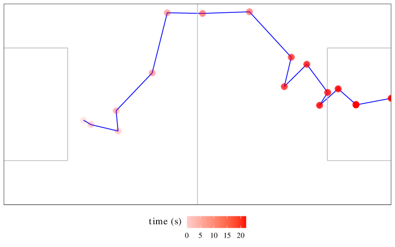
Figure 1: Tracing the locations of the sequence of events that led to the goal scored by Jack Wilshere for Arsenal against Norwich City (voted the best goal of the 2013/14 season).

Figure 1 shows the trajectory of the ball during an attacking move that led to a goal in the 18th minute of the game between Arsenal and Norwich City on October 19, 2013. The goal was scored by Jack Wilshere for Arsenal and was voted as the best goal in the English Premier League for the 2013/14 season.

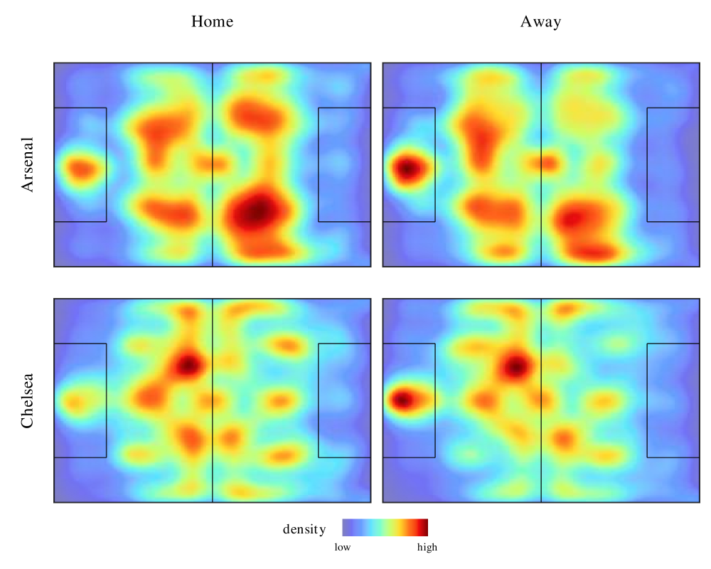
Figure 2: Heat maps showing the density of ball-touches for Arsenal and Chelsea in their home and away games in the 2013/14 season. In all heat maps the team is attacking to the right.

Latent game characteristics, such as the home advantage, and differences in playing styles and formations between the teams are also reflected in the touch-ball events. For example, Figure 2 compares the concentration of ball touches for Arsenal and Chelsea between their home and away games in the 2013/14 season. The playing field is plotted so that the team is always attacking to the right. It is clear that when the teams play at home the density of events is higher towards the opponent’s goal. In fact, the point process modelling framework developed in this paper allows us to quantify home advantage by, for example, learning the relative ability of each team to retain possession when playing at home compared to away (see Section 6.6).

2.2 Data preparation

Table 3: Composite event types along with their labels and observed frequencies in the data.

m	mark label	count
1	Home_Win	10864
2	Home_Dribble	3432
3	Home_Pass_S	152140
4	Home_Pass_U	42344
5	Home_Shot	5127
6	Home_Keeper	3273
7	Home_Save	2208
8	Home_Clear	11780
9	Home_Lose	16534
10	Home_Goal	597
11	Home_Foul	4229
12	Home_Out_Throw	8982
13	Home_Out_GK	3084
14	Home_Out_Corner	2321
15	Home_Pass_O	814

m	mark label	count
16	Away_Win	10829
17	Away_Dribble	3123
18	Away_Pass_S	140975
19	Away_Pass_U	41462
20	Away_Shot	4107
21	Away_Keeper	3555
22	Away_Save	2702
23	Away_Clear	14059
24	Away_Lose	16515
25	Away_Goal	455
26	Away_Foul	4009
27	Away_Out_Throw	8396
28	Away_Out_GK	3697
29	Away_Out_Corner	1779
30	Away_Pass_O	768

We combine the types and outcomes of touch-ball events into in-play and terminal composite events. The in-play composite events are Win, Dribble, Successful Pass (Pass_S), Unsuccessful Pass (Pass_U), Shot, Keeper, Save, Clear and Lose. Win denotes a player regaining possession of the ball from the opponent. Dribble is taking the ball forward with repeated slight touches. Passes are deemed to be successful when the ball is received by a teammate and unsuccessful otherwise. Shots include all attempts on the opponents’ goal, including those missing the target. The Keeper event denotes the goal keeper taking possession of the ball into their hands by picking it up or claiming a cross. The Keeper event is unlike any other in-play event, as the goal keeper is allowed to hold the ball without being challenged for a period of time while waiting for opponents to clear the goal area. As a result, there is often a delay before the next event even though the ball is technically in-play. Saves are events where the goal keeper prevents a shot from crossing the goal line. Clear events are those where a player moves the ball away from their goal area to safety while the Lose event is when a player loses possession of the ball. The terminal composite events are those which result in the ball going out-of-play and are Goal, Foul, Out_Throw, Out_GK, Out_Corner and Offside Pass (Pass_O). The terminal events interrupt the game resulting in a delay before play resumes. Each composite event is tracked for both the home and away teams. For this reason, we append “Home” or “Away” as a prefix to the event label to distinguish between the events of the two teams playing the game. This results in $M=30$ distinct composite events, whose labels and observed frequencies are given in Table 3.

For each touch-ball event, the data also contains the associated $(x,y)$ coordinates on the playing field. We partition the playing field into 3 zones of equal area. The zones and their corresponding labels are shown in Figure 3. Zone 1 is the region where the home team defends their goal, zone 3 is the region where the home team attacks, and zone 2 is the midfield region. It is natural to expect that the control a team has on the game depends on the zone the ball is at. For example, the home team is expected to retain possession of the ball more successfully in zone 1 as compared to zone 3.

Table 4 shows a snapshot of the data after its preparation, including a unique identifier for each game period in the data.

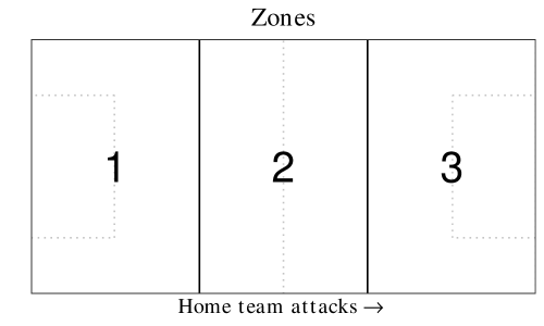
Figure 3: Mapping from event location in $(x,y)$ coordinates to zones.

Table 4: Snapshot of the final data prepared for modelling where each event, indexed by $i=1,...,n$, consists of the following components, the time of occurrence $t_{i}$, the zone $z_{i}$, and the mark $m_{i}$. The home and away team information for each game is assumed to be known and the first event ($t_{1},z_{1},m_{1}$) in each game period is considered to be deterministic and therefore, not modelled.

i	id	period	team_id	time ($t_{i}$)	zone ($z_{i}$)	mark ($m_{i}$)
1	101	1	1	0	2	18
2	101	1	1	1	2	19
3	101	1	2	3	1	8
4	101	1	1	6	3	16
5	101	1	1	8	3	18
6	101	1	1	15	2	18
7	101	1	1	16	1	19
8	101	1	2	19	1	12

3 Marked point processes

3.1 Conditional intensity function

Sequences of events over time are conveniently represented as realisations of a point process. Oftentimes, the events can carry additional information, which are assumed to be realisations of random variables, referred to as marks. The collection of the times $\{t_{i}\}$ at which the events occur and the marks $\{m_{i}\}$ is a marked point process, whose ground process, is the process for $\{t_{i}\}$ only.

A marked point process is typically specified through its joint conditional intensity function

$$\lambda^{*}(t,m)=\lambda^{*}_{g}(t)f^{*}(m\mid t)\,,$$ (1)

where $\lambda^{*}_{g}(t)$ is the conditional intensity of the ground process and $f^{*}(m\mid t)$ is the conditional probability density or mass function of the mark $m$ at time $t$. Both $\lambda^{*}_{g}(t)$ and $f^{*}(m\mid t)$ in (1) are understood as being conditional on $\mathcal{F}_{t^{-}}$, which is the filtration of the marked point process up to but not including $t$.

3.2 Marked Hawkes processes

Marked Hawkes processes are point processes whose defining characteristic is that they self-excite, meaning that each arrival increases the rate of future arrivals for a period of time. More formally, consider a realisation of a marked point process, consisting of event times $\{t_{i}\}$ with $t_{i}\in\mathbb{R}^{+}$ and $t_{i}>t_{i-1}$, and marks $m_{i}\in\{1,\ldots,M\}$ $(i=1,\dots,n)$, where $M$ is the number of discrete marks. The marked Hawkes process is most intuitively specified using its mark dependent conditional intensity function $\lambda^{*}(t,m)$, which for an exponentially decaying intensity is (Rasmussen, 2013, expression 2.2),

$$\lambda^{*}(t,m)=\mu\delta_{m}+\sum_{t_{j}<t}\epsilon\beta\mathrm{e}^{-\beta(t-t_{j})}\gamma_{m_{j}\to m}\,.$$ (2)

In (2), the parameter $\mu>0$ is a constant background intensity and $\delta_{m}\in(0,1)$ is the background mark probability for mark $m$ with $\sum_{m=1}^{M}\delta_{m}=1$. The parameter $\epsilon\in(0,1)$ is the excitation factor, $\beta>0$ is the exponential decay rate and $\gamma_{m_{j}\to m}\in(0,1)$ is the probability the excitation from an event of mark $m_{j}$ triggers an event of mark $m$, with $\sum_{m=1}^{M}\gamma_{m_{j}\to m}=1$ for any $m_{j}\in\{1,\ldots,M\}$.

3.3 Limitations of the marked Hawkes process model

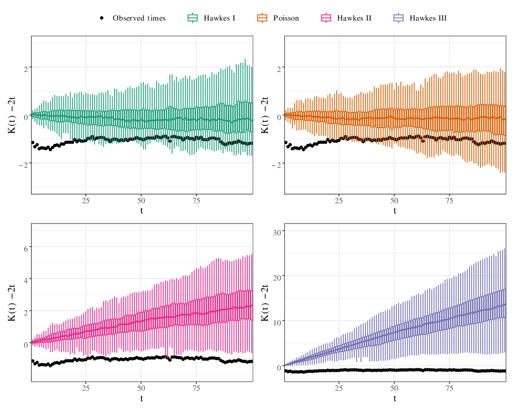
Figure 4: The K function estimate $\hat{K}(t)-2t$ of the observed event times (black points) from the first game of the season between Aston Villa and Arsenal. Hawkes I (green) is a Hawkes process with parameters $(\mu,\epsilon,\beta)=(0.4183,0.0035,0.0004)$ estimated from the observed times using maximum likelihood. A Hawkes process with $\epsilon=0$ is the trivial case with no excitation that reduces to a Poisson process (orange) with estimated rate $\mu=0.4189$. Hawkes II (pink) has parameters $(\mu,\epsilon,\beta)=(0.2594,0.4,0.01)$ and Hawkes III (purple) has parameters $(\mu,\epsilon,\beta)=(0.1068,0.8,0.01)$. Hawkes II and Hawkes III are examples of processes with moderate and severe clustering respectively, whose $\mu$ parameters were estimated from the observed times using maximum likelihood after fixing $\epsilon,\beta$. The box plots of the estimates for the Hawkes and Poisson processes were computed using $100$ independent simulations of each process over the same time interval as the observed times.

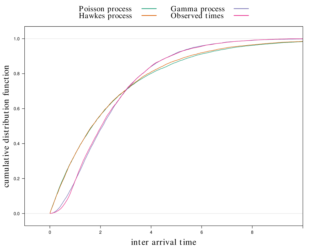
Figure 5: Comparing the cumulative distribution functions (CDFs) of the inter-arrival times of events simulated from a Poisson process (green), a Hawkes process (orange), a Gamma process (purple) and observed event times in football (pink). Empirical CDFs were computed using $10,000$ inter-arrival times in each case.

The specification in (2) describes a marked Hawkes process that is linear in the sense that the excitations from different arrivals add up, not only increasing the probability of triggering an event of a particular type, but also concentrating the occurrence times for a certain period of time. For this reason, marked Hawkes processes have proven useful in a wide range of applications, where events tend to cluster in time, such as the modelling of earthquakes (Ogata, 1998), gang violence (Mohler et al., 2011) and financial market events (Bowsher, 2007).

However, in applications like the modelling of event sequences in football, each event triggers other events of a particular type with high probability, while it is not necessarily true that the occurrence times cluster.

As an illustration that the observed events in football do not exhibit clustering, consider only the collection of the times $\{t_{i}\}$ at which the events occur. A succinct method to investigate the aggregation of the points is using the non-parametric Ripley’s K-function summary (Ripley, 1977), which is the reduced second moment measure. An estimator of the K-function in the one-dimensional case is derived in Diggle (1985) as

$$\hat{K}(t)=\frac{T}{n^{2}}\sum_{i=1}^{n}\sum_{j\neq i}w_{ij}\mathbbm{1}(|t_{i}-t_{j}|\leq t)\,,$$ (3)

where $(0,T)$ is the time interval over which the $n$ points are observed, $\mathbbm{1}(.)$ is the indicator function, and $w_{ij}$ is an edge correction taking values $w_{ij}=1$ if $|t_{i}-t_{j}|\leq\min(t_{i},T-t_{i})$ and $w_{ij}=2$, otherwise.

For a homogeneous Poisson process, $K(t)=2t$. If $K(t)>2t$, the process is said to be over-dispersed relative to the Poisson, and exhibits some degree of clustering. If $K(t)<2t$, the process is under-dispersed relative to the Poisson, and tends towards regular occurrences. Figure 4 shows the K function estimate, $\hat{K}(t)-2t$ for $t\in\{1,2,\ldots,100\}$, of the observed event times from the first game of the season between Aston Villa and Arsenal ($n=1279$). We also compare the estimates from those observed times with the estimates of the events simulated from several one-dimensional Hawkes processes with conditional intensity of the form, $\lambda^{*}(t)=\mu+\sum_{t_{j}<t}\epsilon\beta\mathrm{e}^{-\beta(t-t_{j})}$. Hawkes I (green) is the fitted Hawkes process with parameters $(\mu,\epsilon,\beta)=(0.4183,0.0035,0.0004)$ estimated from the observed times using maximum likelihood. Note that the estimated $\epsilon$ is very close to 0, indicating no clustering. A Hawkes process with $\epsilon=0$ is the trivial case with no excitation that reduces to a Poisson process (orange) with estimated rate $\mu=0.4189$. Hawkes II (pink) has parameters $(\mu,\epsilon,\beta)=(0.2594,0.4,0.01)$ and Hawkes III (purple) has parameters $(\mu,\epsilon,\beta)=(0.1068,0.8,0.01)$. Hawkes II and Hawkes III are examples of processes with moderate and severe clustering respectively, whose $\mu$ parameters were estimated from the observed times using maximum likelihood after fixing $\epsilon,\beta$. The box plots of the estimates for the Hawkes and Poisson processes were computed using $100$ independent simulations of each process over the same time interval as the observed times.

The $\hat{K}(t)-2t$ values for the Hawkes II and Hawkes III processes quickly get above 0 and increase with $t$ demonstrating the behaviour of processes with different degrees of clustering. On the other hand, the $\hat{K}(t)-2t$ values for the fitted Hawkes process (Hawkes I) and the Poisson process concentrate around 0, being indicative of the expected behaviour of processes where points do not cluster. The $\hat{K}(t)-2t$ values from the observed times range from -1.4 to -0.9 indicating slight under-dispersion relative to the Poisson process. In other words, the observed times in football exhibit no clustering and in fact show evidence of being more regular than the Poisson process.

Another method to investigate the aggregation of points is by looking at distribution of the inter-arrival times. Figure 5 shows the empirical distribution function of the first $10,000$ inter-arrival times from the first 7 games of the league season. We also plot the cumulative distribution functions of a homogeneous Poisson process and a Hawkes process, whose parameters are estimated from the aforementioned $10,000$ events using maximum likelihood. The fitted Hawkes process is far from the empirical distribution function, and almost identical to the fitted Poisson process confirming that the arrival times in football do not cluster. This is further evidence that Hawkes processes are not appropriate for modelling events such as those observed in football, that tend not to cluster in time. Figure 5 also includes the cumulative distribution function of a fitted Gamma process, which, as is apparent provides an excellent fit to the observed inter-arrival times.

4 Specification of flexible marked point processes

4.1 Decoupling the modelling of times and marks

According to the decomposition of a multivariate distribution function in Cox (1975, expression 2) the likelihood of a marked point process observed in $(0,T)$ can always be factorised as

$$\mathcal{L}(\mathcal{F}_{t_{n}}\mid\bm{\zeta},\bm{\theta})=\prod_{i=1}^{n}\left\{g(t_{i}\mid\mathcal{F}_{t_{i-1}};\bm{\zeta})f(m_{i}\mid t_{i},\mathcal{F}_{t_{i-1}};\bm{\theta})\right\}\left\{1-G(T\mid\mathcal{F}_{t_{n}};{\bm{\zeta}})\right\}\,,$$ (4)

where $g$, $G$, and $f$ are the conditional density and distribution function for the times, and the probability mass function for the marks, respectively, and $\bm{\zeta},\bm{\theta}$ are unknown parameter vectors that may or may not share components. The last term in (4) accounts for the fact that the unobserved occurrence time $t_{n+1}$ must be after the end of the observation interval $(0,T)$. Therefore, an alternative approach to specify a marked point process is to specify the functions $g(\cdot\mid\mathcal{F}_{t_{i-1}};\bm{\zeta})$ and $f(\cdot\mid t_{i},\mathcal{F}_{t_{i-1}};\bm{\theta})$, separately, and combine them as in (4). The key insight in the current work is to derive the specification for the marks $f(\cdot\mid t_{i},\mathcal{F}_{t_{i-1}};\bm{\theta})$ from the joint conditional intensity function of a marked Hawkes process model, and then to specify a probability density function for the times $g(\cdot\mid\mathcal{F}_{t_{i-1}};\bm{\zeta})$ best suited to our application. In this way, we can restrict the characteristic excitation property of marked Hawkes processes exclusively to the modelling of the marks, and have the freedom to specify a different model for the occurrence times.

By the definition of the conditional intensity function for a marked point process in (1), $f(m_{i}\mid t_{i},\mathcal{F}_{t_{i-1}};\bm{\theta})=\lambda^{*}(t_{i},m_{i})/\sum_{m=1}^{M}\lambda^{*}(t_{i},m)$. Plugging in $\lambda^{*}(t_{i},m)$ from (2) in the latter expression, gives

$$f(m_{i}\mid t_{i},\mathcal{F}_{t_{i-1}};\bm{\theta})=\frac{\delta_{m_{i}}+\sum_{t_{j}<t_{i}}\alpha^{*}\mathrm{e}^{-\beta(t_{i}-t_{j})}\gamma_{m_{j}\to m_{i}}}{1+\sum_{t_{j}<t_{i}}\alpha^{*}\mathrm{e}^{-\beta(t_{i}-t_{j})}}\,,$$ (5)

where $\alpha^{*}=\frac{\epsilon\beta}{\mu}$. Expression (5) makes it immediately apparent, that the parameters $\mu$ and $\epsilon$ of the marked Hawkes process as specified by (2) are not always identifiable for general specifications of $g(\cdot\mid\mathcal{F}_{t_{i-1}};\bm{\zeta})$ in (4). Apart from a mathematical fact, this is also rather intuitive, because $\mu$ and $\epsilon$ in  (2) characterise the evolution of the Hawkes process in the time dimension and the sequence of marks is not sufficient to identify them.

The specification of the marked point process likelihood is complete once a probability density function $g(\cdot\mid\mathcal{F}_{t_{i-1}};\bm{\zeta})$ for the event times is specified.

We should highlight here that the marked point processes from the factorisation in (4) are generally different to the ones that result by assuming separability of the conditional intensity functions (see, for example, González et al., 2016, Section 6.5). A separable conditional intensity functions has the form

$$\lambda^{*}(t,m)=\lambda^{*}_{g}(t)f^{*}(m)\,.$$

and implies that the conditional distribution of the mark does not depend on the occurrence time $t$. Separability is a convenient assumption because it allows for the sequence of marks to be modelled separately from the sequence of times. In contrast, the factorisation in (4) allows the conditional distribution of the mark to depend on the time of occurrence as well as the history, still allowing for estimating ${\bm{\theta}}$ separately from ${\bm{\zeta}}$, if ${\bm{\theta}}$ and ${\bm{\zeta}}$ do not share components.

The proposed marked point process model also allows the recovery of the hidden branching structure of the process, a key feature of Hawkes Processes (Hawkes and Oakes, 1974). In Section 6.8, we calculate the branching structure probabilities and quantify the relative contributions of the background process and previous occurrences to the triggering of a new event.

4.2 Parameter interpretation

In (5), the mark probability of each event in the sequence is determined by a combined additive effect from a background component and all previous occurrences. The first term $\delta_{m_{i}}$ in the numerator is the mark probability associated with the background component, while each term $\alpha^{*}\mathrm{e}^{-\beta(t_{i}-t_{j})}\gamma_{m_{j}\to m_{i}}$ is the contribution from the excitation caused by a previous occurrence in the sequence.

The background mark probability $\delta_{m}\in(0,1)$ is the probability an event has a mark $m$ if the event is triggered solely by the background component. The excitation factor $\alpha^{*}\geq 0$ is a scaling factor applied to the contributions from the previous occurrences to the event mark probability. Large values of $\alpha^{*}$ indicate a stronger dependence of the process on its history, because the contributions from previous occurrences are weighted higher relative to the background component. The decay rate $\beta>0$ is the exponential rate at which the excitations from previous occurrences decay over time. The parameter $\gamma_{m_{j}\to m_{i}}\in(0,1)$ is the probability the excitation from an event of mark $m_{j}$ triggers an event of mark $m_{i}$. In other words, $\gamma_{m_{j}\to m_{i}}$ can be viewed as the conversion rate for the transition from an event with mark $m_{j}$ to an event with mark $m_{i}$.

In summary, as in marked Hawkes processes, the specification for the marks in (5) captures not only all cross-excitations between the various marks but also the rate at which these excitations decay over time.

4.3 Covariate-driven cross excitation

The conditional distribution of marks with probability mass function (5), allows to drive the cross-excitation of the marks using covariates. The conversion rates $\gamma_{m_{j}\to m}$ can be linked to a covariate vector ${\bm{x}}=(x_{1},\ldots,x_{p})^{\top}$ observed at the current time through the baseline-category logit specification (see, for example, Agresti, 2007, Section 6.1)

$$\log\left(\frac{\gamma_{m_{j}\to m}}{\gamma_{m_{j}\to M}}\right)=\phi_{m_{j}\to m}+{\bm{\omega}}_{m}^{\top}{\bm{x}}\qquad(m=1,\ldots,M-1)\,,$$ (6)

where ${\bm{\omega}}_{m}$ is an unknown $p$-vector of regression parameters. Then, keeping all covariates apart from $x_{t}$ fixed, $\omega_{mt}$ is the log of the ratio of odds for category $m$ versus the baseline category $M$ at $x_{t}+1$ to that at $x_{t}$ $(t=1,\ldots,p)$. Also, by setting all covariates $x_{t}$ equal to 0, $\phi_{m_{j}\to m_{i}}$ is the log of the ratio of odds for category $m$ versus the baseline category $M$. The covariate vector ${\bm{x}}$ can include a combination of process-specific covariates that are time-invariant, and event-specific covariates. For example, in Section 5.2, we use (6) to parameterise the marked point process in terms of the relative abilities of teams for each event type, and produce team rankings per event-type.

4.4 Spatio-temporal marked point processes

We can readily extend the factorisation of the likelihood in (4) to include conditional densities for the event locations, when the latter are observed. We can write

$$\mathcal{L}(\mathcal{F}_{t_{n}}\mid\bm{\psi})=\prod_{i=1}^{n}\left\{g(t_{i}\mid\mathcal{F}_{t_{i-1}};\bm{\zeta})h(z_{i}\mid t_{i},\mathcal{F}_{t_{i-1}};\bm{\eta})f(m_{i}\mid t_{i},z_{i},\mathcal{F}_{t_{i-1}};\bm{\theta})\right\}\left\{1-G(T\mid\mathcal{F}_{t_{n}};{\bm{\zeta}})\right\}\,,$$ (7)

where $\{z_{i}\}$ is the collection of random variables corresponding to the spatial component of the process, which is characterised by the conditional probability mass or density functions $h(\cdot\mid t_{i},\mathcal{F}_{t_{i-1}};\bm{\eta})$ with $\bm{\eta}$ being a parameter vector that may or may not share parameters with $\bm{\zeta}$ and $\bm{\theta}$, and $\bm{\psi}=(\bm{\zeta}^{\top},\bm{\eta}^{\top},\bm{\theta}^{\top})^{\top}$. The filtration $\mathcal{F}_{t_{i}}$ now includes all times, marks and locations up to time $t_{i}$.

If the process ends at the last occurrence time $t_{n}$, then the last term $1-G(T\mid\mathcal{F}_{t_{n}};{\bm{\zeta}})$ in (4) and (7) is not part of the likelihood (see, for example Lindqvist, 2006, Section 4.2). This is the case in the modelling of touch-ball event sequences in football we consider here, where the process ends with or immediately after the last event observed in each half of the game.

5 Bayesian modelling of in-game event sequences

5.1 Preamble

The framework for specifying flexible marked point processes of Section 4 is rather attractive for the modelling of in-game event sequences in football and other team sports. Firstly, cross-excitation of in-game events is a natural assumption because any event in an event sequence is likely to be triggered by one or more of the previous events. For example, following a corner kick, the next event is with high probability one among a shot on goal, a defensive clearance or a claim by the keeper. Such effects can be naturally and readily captured by the parameters of the conditional mark distribution in (5), which involves not only the magnitudes of all cross-excitations between the various event types but also the rate at which these excitations decay over time. Secondly, the preliminary analyses in Section 3.3 provides strong evidence that occurrence times do not necessarily cluster, as off-the-shelf marked Hawkes processes imply. Hence, the freedom to use a more flexible conditional distribution for the occurrence times, such as a Gamma process, is a rather attractive prospect. Furthermore, as discussed in Section 4.3, team information can be incorporated in the model in a direct way as covariate information to drive the cross-excitation based on the relative abilities of the teams.

Overall, as we demonstrate later, the framework of Section 4 can be used to provide valuable explanatory tools into the underlying dynamics of the game for the coaching staff and inform strategic decision making. It can also produce predictions of events, such as goals, in a specified time horizon, and of game outcomes that can enhance, among other things, the viewing experience in televised games.

5.2 Excitation-based models

Assume that the touch-ball events in $S$ game periods are $S$ realisations of independent spatio-temporal point processes, with the $s$th realisation involving $n_{s}$ events. Denote by $t_{si}$, $m_{si}$, and $z_{si}$ the occurrence time, mark and location of the $i$-th event in the $s$th realisation, respectively. Each of the $S$ independent spatio-temporal marked point processes has a likelihood as in (7) after dropping the last term, and with conditional probability mass function for the marks as in (5). The product of the $S$ likelihoods is the overall likelihood based on the $S$ game periods.

The probability density functions for the occurrence times within each period are set to

$$g(t_{si}\mid\mathcal{F}_{st_{si-1}};\bm{\zeta}) =p(t_{si}-t_{si-1}\mid m_{si-1},\bm{a},\bm{b})$$

$$t_{si}-t_{si-1}\mid m_{si-1},\bm{a},\bm{b} \sim\text{Gamma}(a_{m_{si-1}},b_{m_{si-1}})\,,$$ (8)

where $\mathcal{F}_{st_{si}}$ denotes the filtration of the $s$th process up to time $t_{si}$.

By this specification, the time to next event is modelled using a gamma distribution with shape and rate parameters that are specific to the mark of the last observed event. In this way, we wish to capture the differences in the expected time to the next event across the different event types. For example, we expect a shorter time to the next event after an in-play event like a Pass, compared to that of an out-of-play event like a Foul. Even within the group of out-of-play events, we expect a shorter delay following a Throw-in as compared to a Goal event.

For a discrete set of locations $\{1,\ldots,Z\}$, the conditional probability mass function for the current location is set to

$$h(z_{si}\mid t_{si},\mathcal{F}_{st_{si-1}};\bm{\eta}) =\eta_{(z_{si-1},\mathop{m_{si-1}})\to z_{si}}\,,$$ (9)

where $\eta_{(z_{si-1},\mathop{m_{si-1}})\to z_{si}}$ is the probability of transitioning into location $z_{si}$ given the location $z_{si-1}$ and the mark $m_{si-1}$ of the last observed event. Expression (9) models the sequence of locations as a discrete first-order Markov chain (see, for example, Norris, 1997) with a transition probability matrix $\bm{\eta}$. The current state of the Markov chain is determined by the combination of the location and the mark of the last observed event, and the probability of transitioning into the next location depends only on the current state. The state space of the Markov chain is given by the Cartesian product $\{1,\dots,Z\}\times\{1,\dots,M\}$.

We consider four alternative parameterisations for the conditional probability mass function for the marks. The S$\beta$ (scalar $\beta$) spatio-temporal marked point process results from (8), (9) and a conditional mark distribution of the form (5), that is

$$f(m_{si}\mid t_{si},\mathcal{F}_{st_{si-1}};\bm{\theta})=\frac{\delta_{m_{si}}+\sum_{t_{sj}<t_{si}}\mathrm{e}^{\alpha-\beta(t_{si}-t_{sj})}\gamma_{m_{sj}\to m_{si}}}{1+\sum_{t_{sj}<t_{si}}\mathrm{e}^{\alpha-\beta(t_{si}-t_{sj})}}\,,$$ (10)

where $\alpha=\log(\alpha^{*})$. The V$\beta$ (vector $\beta$) model results from (8), (9) and

$$f(m_{si}\mid t_{i},\mathcal{F}_{st_{si-1}};\bm{\theta})=\frac{\delta_{m_{si}}+\sum_{t_{sj}<t_{si}}\mathrm{e}^{\alpha-\beta_{m_{sj}}(t_{si}-t_{sj})}\gamma_{m_{sj}\to m_{si}}}{1+\sum_{t_{sj}<t_{si}}\mathrm{e}^{\alpha-\beta_{m_{sj}}(t_{si}-t_{sj})}}\,,$$ (11)

where $\beta_{m}$ is the exponential decay rate of the excitation caused by an event of mark $m$. V$\beta$ allows the decay rates to depend on the mark of the event causing the excitation. Hence, S$\beta$ is formally nested in V$\beta$ and results when $\beta=\beta_{1}=\ldots=\beta_{M}$. The M$\beta$ (matrix $\beta$) process results from (8), (9) and

$$f(m_{si}\mid t_{si},z_{si},\mathcal{F}_{st_{si-1}};\bm{\theta})=\frac{\delta_{m_{si}\mid z_{si}}+\sum_{t_{sj}<t_{si}}\mathrm{e}^{\alpha-\beta_{m_{sj}\to m_{si}\mid z_{si}}(t_{si}-t_{sj})}\gamma_{m_{sj}\to m_{si}\mid z_{si}}}{\sum_{m=1}^{M}\left[{\delta_{m\mid z_{si}}+\sum_{t_{sj}<t_{si}}\mathrm{e}^{\alpha-\beta_{m_{sj}\to m\mid z_{si}}(t_{si}-t_{sj})}\gamma_{m_{sj}\to m\mid z_{si}}}\right]}\,,$$ (12)

where $\beta_{m\to m^{\prime}\mid z}$ is the decay rate of the excitation caused by an event of mark $m$ on an event of mark $m^{\prime}$ at location $z$. Specification (12) allows the decay rates to vary both with the pair of marks involved in the excitation and across locations, and allows the background mark probabilities $\bm{\delta}$ and event conversion rates $\bm{\gamma}$ to vary across location. The M$\beta$ model can be used to account for scenarios like those where a Corner event excites a Pass event in the short term and a Shot event in the longer term ($\beta_{\textsf{Corner}\to\textsf{Pass}\mid 3}>\beta_{\textsf{Corner}\to\textsf{Shot}\mid 3}$). It also allows us to capture effects such as how a team is more likely to make more passes and retain possession of the ball in the defensive zone, while attempting more shots on goal in the attacking zone ($\gamma_{\textsf{Pass}\to\textsf{Pass}\mid 1}>\gamma_{\textsf{Pass}\to\textsf{Pass}\mid 3}$ and $\gamma_{\textsf{Pass}\to\textsf{Shot}\mid 3}>\gamma_{\textsf{Pass}\to\textsf{Shot}\mid 2}$). The final model we consider is the M$\beta$A (matrix $\beta$ with abilities) where the baseline category logits of the conversion rates in (6) are driven by team information as

$$\log\left(\frac{\gamma_{m_{sj}\to m\mid z}(c)}{\gamma_{m_{sj}\to M\mid z}(c)}\right)=\phi_{m_{sj}\to m\mid z}+\omega_{cm}\quad(m=1,\dots,M-1;c=1,\ldots,C)\,.$$ (13)

In the above expression, $\phi_{m\to m^{\prime}\mid z}$ is a location-dependent baseline conversion, and $c$ is the team in possession of the ball attempting the event conversion. The parameter $\omega_{cm}$, then, reflects the ability of a team to complete a conversion to an event of mark $m$.

5.3 Prior distributions

The shape and rate parameters of the Gamma distributions for the inter-arrival times in (8) are assigned independent exponential priors with rates $a^{\prime}$ and $b^{\prime}$, respectively. The probability mass function for the locations specified in (9) models the locations as a multinomial distribution given the current state of the Markov chain. The conjugate prior for the multinomial distribution is the Dirichlet distribution (see, for example, Gelman et al., 2013, Section 3.4) and therefore we assign a Dirichlet prior on the multinomial probabilities $\bm{\eta}$ with a common concentration rate parameter $\nu$. The background mark probability vector $\bm{\delta}$ in the S$\beta$, V$\beta$, M$\beta$ and M$\beta$A models is also assigned a Dirichlet prior with concentration hyper-parameter $\delta^{\prime}$. The location-specific mark probability vectors $(\delta_{1\mid 1},\ldots,\delta_{M\mid 1})^{\top},\ldots,(\delta_{1\mid Z},\ldots,\delta_{M\mid Z})^{\top}$ in the M$\beta$ and M$\beta$A models are assigned independent Dirichlet priors with concentration hyper-parameter $\delta^{\prime\prime}$. The excitation factor $\alpha$ is assigned a normal prior with mean $0$ and standard deviation $\sigma_{\alpha}$. The decay rate parameter $\beta$ in the S$\beta$ model, the parameters $\beta_{1},\ldots,\beta_{M}$ in the V$\beta$ model, and their location-specific counterparts in the M$\beta$ and M$\beta$A models are assigned independent exponential priors with a common rate $\beta^{\prime}$. The parameters $\phi_{m\to m^{\prime}\mid z}$ and $\omega_{cm}$ $(m,m^{\prime}=1,\ldots,M;z=1,\ldots,Z;c=1,\ldots,C)$ in the M$\beta$A model are assigned independent Normal priors with mean $0$ and standard error $\sigma_{\gamma}$. The conversion rate parameters $(\gamma_{m\to 1},\ldots,\gamma_{m\to M})^{\top}$ in the S$\beta$ and V$\beta$ models, and their location-specific counterparts in the M$\beta$ model are assigned independent Dirichlet priors with a common concentration rate parameter $\gamma^{\prime}$.

5.4 Posterior distributions

The time and location conditional distributions corresponding to (8) and (9) share no parameters with each other, and no parameters with any of the conditional mark distributions for the S$\beta$, V$\beta$, M$\beta$, and M$\beta$A models. Furthermore, the likelihood in (7) can be factorised into a term depending only on the time parameters $\bm{\zeta}$, a term depending only on the location parameters $\bm{\eta}$ and a term depending only on the mark parameters $\bm{\theta}$. Given that the priors for $\bm{\zeta}$, $\bm{\eta}$ and $\bm{\theta}$ are also independent, the derivation of, or sampling from, the posterior distributions can be performed separately for each of those parameters.

The priors for the location parameters $\bm{\eta}$ are conjugate, so the posterior for $\bm{\eta}$ is readily obtained. If $\bm{y}=\{y_{i\to j}\}$, for $j\in\{1,\dots,Z\}$, are the observed counts of transitions originating from the state $i$ where $i\in\{1,\dots,Z\}\times\{1,\dots,M\}$, then the posterior distribution of each row of the transition matrix $\bm{\eta_{i}}$ is a Dirichlet distribution with concentration parameters $(y_{i1}+\nu,\ldots,y_{iZ}+\nu)$.

Posterior sampling for the parameter vectors $\bm{a}$, $\bm{b}$ in (8) of the conditional distributions for the times, and the parameters $\bm{\theta}$ of the conditional distributions for the marks in each of the S$\beta$, V$\beta$, M$\beta$, and M$\beta$A models is carried out using the variant of the Hamiltonian Monte Carlo procedure (Duane et al., 1987) that is implemented in Stan (Stan Development Team, 2020).

We have also implemented posterior sampling using a Metropolis-within-Gibbs procedure, which, though, proved to mix poorly in artificial data sets for the S$\beta$, V$\beta$, M$\beta$, and M$\beta$A, rendering it computationally infeasible. As in the case of Hawkes process, the poor mixing stems from the presence of strong correlations between the model parameters as well as the flatness of the likelihood function (Veen and Schoenberg, 2008). Stan, on the other hand, implements the No-U-Turn Sampler (Hoffman and Gelman, 2014) that automatically calibrates tuning parameters in a warm-up phase and can efficiently sample from complex posterior distributions.

5.5 Model complexity

The conditional mark distribution in the M$\beta$ and M$\beta$A models involves a large number of parameters. There are $M^{2}Z$ decay rate parameters and $M(M-1)Z$ baseline conversion rate parameters which makes posterior sampling a computationally challenging task. We have developed a screening procedure based on association rule learning (see, for example, Agrawal et al., 1993) that operates on the data involved in the likelihood and eliminates parameters prior to posterior sampling.

The screening procedure retains only those parameters that capture the most significant event interactions and depends on two constants that need to be chosen. The first is the window size $W$ for the number of transient events, and any event is allowed to be triggered by only one of the $W$ events leading up to it. The other is the number of event pairs $N$ considered in each of the three zones and sets a threshold on the number of significant event interactions that are identified. Full details on the association rule based screening procedure are given in Section S2 of the Supporting Materials.

5.6 Model evaluation

Let ${\bm{X}}^{(train)}$ be the set of the training data on which the likelihood is based on, consisting of $n^{(train)}$ events, and let $\bm{\psi}^{(1)},\ldots,\bm{\psi}^{(R)}$ be $R$ samples from the posterior distribution. Denote by ${\bm{X}}^{(test)}$ the set of held-out test data, consisting of $n^{(test)}$ events.

One method to evaluate the predictive accuracy of each model is to use the log point-wise predictive density (Vehtari et al., 2017) computed on the test data, using the posterior samples

$$\widehat{lpd}=\sum_{(t,z,m)\in{\bm{X}}^{(test)}}\log\left(\frac{1}{R}\sum_{r=1}^{R}L(t,z,m\mid\mathcal{F}_{t^{-}},\bm{\zeta}^{(r)},\bm{\eta}^{(r)},\bm{\theta}^{(r)})\right)\,,$$ (14)

where $L(t,z,m\mid\mathcal{F}_{t^{-}},\bm{\zeta}^{(r)},\bm{\eta}^{(r)},\bm{\theta}^{(r)})$ is the likelihood of $(t,z,m)$ given the filtration $\mathcal{F}_{t^{-}}$ at the posterior sample $\bm{\zeta}^{(r)},\bm{\eta}^{(r)},\bm{\theta}^{(r)}$. Large values of $\widehat{lpd}$ indicate better predictive accuracy.

Apart from S$\beta$, V$\beta$, M$\beta$, and M$\beta$A, we also evaluate the predictive accuracy of two simpler baseline models that do not include Hawkes-like excitation effects. The first baseline model, termed FOMC model, is based on the factorisation of the likelihood of marked spatio-temporal processes in expression (7) with models for the times and locations as in (8) and (9), respectively, but with the conditional probability mass function for the marks being a first-order Markov chain

$$f(m_{i}\mid t_{i},z_{i},\mathcal{F}_{t_{i-1}};\bm{\theta})=\theta_{(z_{i},\mathop{m_{i-1}})\to m_{i}}\,.$$ (15)

In this specification, $\theta_{(z,\mathop{m})\to m^{\prime}}$ is the probability of the event mark $m^{\prime}$ given that last observed event has location $z$ and mark $m$. The second baseline model, termed MSTHP, is the marked spatio-temporal homogeneous Poisson process (Daley and Vere-Jones 2003, Section 7.3), which has likelihood

$$\mathcal{L}^{(P)}(\bm{q}\mid\bm{\rho})=\prod_{m=1}^{M}\prod_{z=1}^{Z}\rho_{mz}^{q_{mz}}\exp\left\{-T\rho_{mz}\right\}\,,$$ (16)

where $\rho_{mz}$ is the Poisson rate parameter and $q_{mz}$ is the number of event occurrences for mark $m$ at location $z$ over a total observation time $T$ in the data.

The FOMC and MSTHP models have conjugate prior distributions and therefore their posteriors are readily obtained. Details on those prior distributions and the derivation of their posterior distributions are given in Section S1 of the Supporting Materials.

Table 5: Zone-wise frequencies for each event type in the training data.

Home
mark		zone
m	label	1	2	3
1	Home_Win	236	257	41
2	Home_Dribble	17	96	96
3	Home_Pass_S	1699	4633	1658
4	Home_Pass_U	541	825	725
5	Home_Shot	0	0	292
6	Home_Keeper	155	0	0
7	Home_Save	106	0	0
8	Home_Clear	557	141	32
9	Home_Lose	122	287	368
10	Home_Goal	0	0	22
11	Home_Foul	62	126	64
12	Home_Out_Throw	97	184	163
13	Home_Out_GK	149	0	0
14	Home_Out_Corner	0	0	112
15	Home_Pass_O	7	19	20

Away
mark		zone
m	label	1	2	3
16	Away_Win	25	204	301
17	Away_Dribble	76	65	19
18	Away_Pass_S	1427	4390	2030
19	Away_Pass_U	542	811	702
20	Away_Shot	193	2	0
21	Away_Keeper	0	0	192
22	Away_Save	0	0	149
23	Away_Clear	27	124	660
24	Away_Lose	323	349	142
25	Away_Goal	20	0	0
26	Away_Foul	46	112	69
27	Away_Out_Throw	143	173	110
28	Away_Out_GK	0	0	220
29	Away_Out_Corner	76	0	0
30	Away_Pass_O	13	11	5

6 Explanatory modelling

Table 6: Posterior summaries and convergence diagnostics from 2000 posterior samples for selected parameters from the M$\beta$A model after screening with $(W,N)=(5,100)$.

parameter	mean	sd	$\hat{R}$	$N^{(eff)}$
$\beta_{3\to 3\mid 1}$	0.52	0.04	1.00	1309.81
$\beta_{27\to 8\mid 1}$	1.97	0.86	1.00	1953.81
$\beta_{24\to 1\mid 2}$	1.51	0.09	1.00	2042.84
$\beta_{3\to 4\mid 2}$	0.65	0.03	1.01	913.52
$\beta_{3\to 5\mid 3}$	0.63	0.04	1.01	1933.43
$\beta_{3\to 10\mid 3}$	0.81	0.24	1.01	882.31
$\phi_{3\to 3\mid 1}$	1.70	0.50	1.01	792.46
$\phi_{27\to 8\mid 1}$	-0.74	0.87	1.00	2159.96
$\phi_{24\to 1\mid 2}$	3.29	0.37	1.02	539.25

parameter	mean	sd	$\hat{R}$	$N^{(eff)}$
$\phi_{3\to 4\mid 2}$	1.81	0.41	1.01	540.41
$\phi_{3\to 5\mid 3}$	1.38	0.35	1.01	576.16
$\phi_{3\to 10\mid 3}$	-1.31	0.59	1.01	1098.83
$\delta_{3\mid 1}$	0.56	0.03	1.00	1805.80
$\delta_{3\mid 2}$	0.24	0.08	1.00	1356.85
$\delta_{3\mid 3}$	0.03	0.01	1.00	2207.39
$\alpha$	6.30	0.09	1.01	866.96
$\omega_{9,3}$	0.59	0.26	1.03	334.15
$\omega_{10,3}$	0.67	0.25	1.01	341.24

6.1 Training

Samples from the posterior distributions for the parameters of the S$\beta$, V$\beta$, M$\beta$, and M$\beta$A models of Section 5.2, and of the FOMC and MSTHP baseline models of Section 5.6 are obtained using all event sequences from the first $20$ games of the league season, played between 17/08/2013 and 26/08/2013, which constitute $\bm{X}^{(train)}$. The training data involves $S=40$ game periods involving of $27,660$ events. Each of the $20$ teams participating in the league plays in two of the $20$ games, one at their home and one at their away venue. As is also described in Section 2.1, there are $M=30$ marks and $Z=3$ zones. Table 5 gives the zone-wise event frequencies across marks in the training data used for modelling, reflecting the large variability in the frequencies both across marks and zones.

For the M$\beta$ and M$\beta$A models, the association rule learning screening procedure of Section 5.5 is employed for all combinations of $W\in\{5,10\}$ and $N\in\{50,100\}$ to eliminate some of the model parameters and reduce the model complexity before posterior sampling.

The hyper-parameters for the prior distributions specified in Section 5.3 are as follows. The hyper-parameters $a^{\prime}$ and $b^{\prime}$ for the exponential priors on the parameters of the Gamma distributions in (8) are both set to $0.01$. The Dirichlet prior on the background mark probabilities $\bm{\delta}$ has concentration hyper-parameter $\delta^{\prime}=1$. The exponential prior on the decay rates $\bm{\beta}$ has a rate hyper-parameter $\beta^{\prime}=0.1$. The Normal priors on the excitation factor $\alpha$ and the baseline-category logit model parameters $\bm{\phi}$ and $\bm{\omega}$ have hyper-parameters $\sigma_{\alpha},\sigma_{\gamma}=10$. The location-specific background mark probability vectors in the M$\beta$ and M$\beta$A models are assigned independent Dirichlet priors with concentration hyper-parameter $\delta^{\prime\prime}=1$.

The ability parameters in the baseline category logit specification for the conversion rates of the M$\beta$A are not directly identifiable. In order to make them so, we set the abilities $\omega_{cm}$ for West Ham United to $0$ $(m=1,\ldots,30)$. Then, $\omega_{cm}>0$ indicates that for team $c$, a previous event is more likely to trigger an event of mark $m$ when compared to the reference team.

Samples from the posterior distributions are obtained by running four parallel chains using the Hamiltonian Monte Carlo procedures implemented in Stan. The Stan templates we used are all provided in the Supporting Materials. Each chain is initialised with different starting values and run for a total of 500 iterations post the warm-up phase. Table 6 gives posterior summaries along with convergence diagnostics for some of the parameters of the M$\beta$A model with $W=5$ and $N=100$; the corresponding chain-wise trace plots are provided in the Supporting Materials.

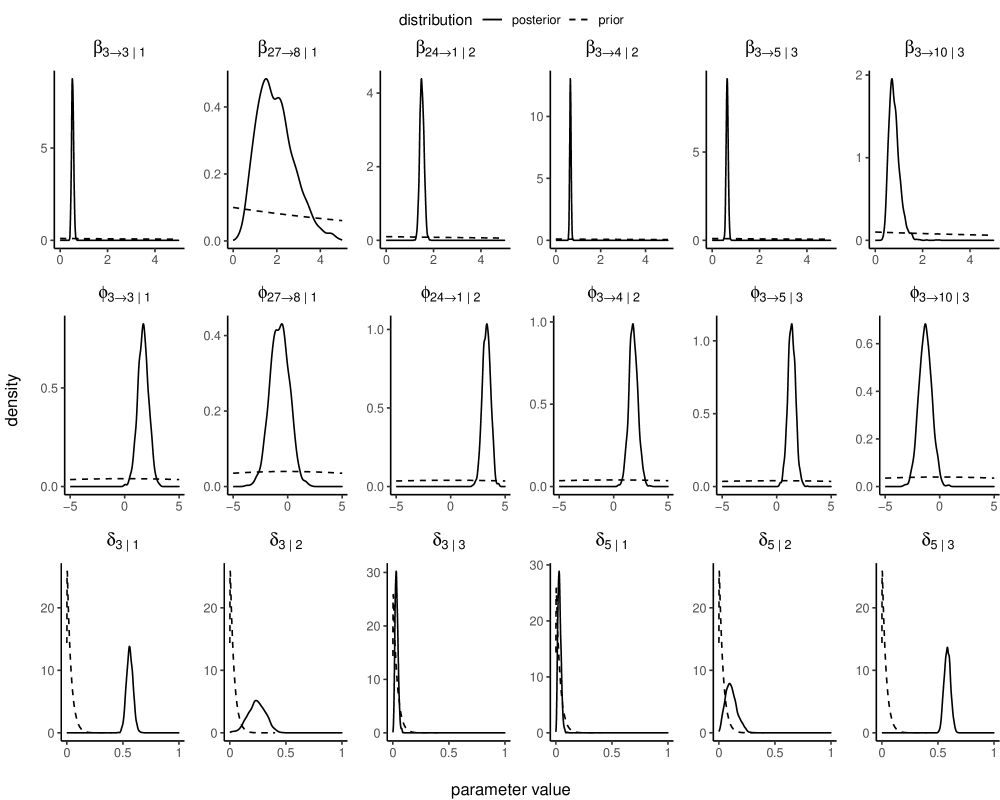
Figure 6: Visualising the impact of prior specifications by overlaying the posterior and prior densities for selected model parameters for the M$\beta$A model with $(W,N)=(5,100)$.

The convergence of the algorithm is assessed using the potential scale reduction factor $\hat{R}$ proposed by Gelman et al. (1992), which is the ratio of the average variance within each chain to the variance of the aggregated samples across chains. If the chains have converged to the stationary distribution, the expected value of $\hat{R}$ is 1. All parameters have $\hat{R}<1.1$, which, as recommended in Gelman et al. (1992), is evidence for convergence. Table 6 also gives the effective sample size (see, for example, Gelman et al., 2013, Section 11.5) for the samples for each of the posterior marginals, which indicate that the sampler returned samples with acceptable autocorrelation. For some parameters the effective sample size is larger than the sample size due to negative autocorrelations. This, as pointed out in Vehtari et al. (2021), is a consequence of the HMC algorithm used in Stan being an antithetic Markov chain which has negative autocorrelations on odd lags. The impact of the prior distributions in Section 5.3 on the posterior samples is minimal as seen, for a selection of parameters, in Figure 6 indicating that the posterior distributions of the parameters have concentrated after accounting for the likelihood.

Table 7: Cumulative log posterior densities $\widehat{lpd}$ over 10 game periods in the test data for all fitted models along with the number of estimated parameters $d^{(par)}$ in each model. For the M$\beta$ models, $W$ is the number of transient events and $N$ is the number of significant event pairs identified in the rule-based framework for reducing model complexity.

model	abbreviation	$d^{(par)}$	$\widehat{lpd}$
Homogeneous Poisson process (Baseline)	MSTHP	90	-35469.50
Matrix $\beta$ $(W,N)=(10,50)$	M$\beta$2	538	-22288.64
Matrix $\beta$ $(W,N)=(5,50)$	M$\beta$1	538	-22152.08
First order Markov chain (Baseline)	FOMC	870	-21898.31
Scalar $\beta$	S$\beta$	902	-21838.04
Vector $\beta$	V$\beta$	915	-21829.81
Matrix $\beta$ with abilities $(W,N)=(5,100)$	M$\beta$A	1539	-21599.81
Matrix $\beta$ $(W,N)=(10,100)$	M$\beta$4	988	-21496.56
Matrix $\beta$ $(W,N)=(5,100)$	M$\beta$3	988	-21342.57

6.2 Model evaluation

The S$\beta$, V$\beta$, M$\beta$, and M$\beta$A models are compared with each other and with the FOMC and MSTHP baseline models of Section 5.6 in terms of their log point-wise predictive density (14) computed on test data. The test data $\bm{X}^{(test)}$ includes all events from the 5 games immediately following the games in the training data, played between 31/08/2013 and 01/09/2013. The test data involves $S=10$ game periods involving of $27,660$ events.

Table 7 gives the log predictive densities $\widehat{lpd}$, summed over all the events in the $10$ game periods in the test data. Table 7 also provides the number of parameters in each model as a measure of their complexity. The three top performing models are the M$\beta$ model after screening with $(W,N)=(5,100)$, followed by M$\beta$ model after screening with $(W,N)=(10,100)$, and M$\beta$A with $(W,N)=(5,100)$. Notably, the M$\beta$ model after screening with $(W,N)=(5,100)$ performs the best among the list of fitted models, significantly outperforming also models of similar complexity, such as the S$\beta$, V$\beta$ and FOMC models. The slightly poorer performance of the M$\beta$A model with $(W,N)=(5,100)$ is most probably due to the fact that, in the training data, each team plays just one game at their home and one at their away venue. Nevertheless, in order to illustrate the full explanatory potential of the modelling framework in Section 4, we focus on inferences based on the posterior samples from the M$\beta$A model.

6.3 Background mark probabilities

Table 8: Posterior means and standard deviations (in parenthesis) of the zone dependent background mark probabilities $\delta_{m\mid z}$ for $z\in\{1,2,3\}$ from the M$\beta$A model. The dots ($\cdot$) denote means and standard deviations less than 0.005.

mark label	1	2	3
Home_Win	.	.	.
Home_Dribble	.	0.01 (0.01)	.
Home_Pass_S	0.56 (0.03)	0.24 (0.08)	0.03 (0.01)
Home_Pass_U	0.06 (0.01)	0.04 (0.02)	0.03 (0.01)
Home_Shot	.	.	.
Home_Keeper	0.04 (0.01)	.	.
Home_Save	.	.	.
Home_Clear	0.05 (0.02)	.	.
Home_Lose	.	0.04 (0.02)	.
Home_Goal	.	.	.
Home_Foul	0.03 (0.01)	0.09 (0.04)	0.02 (0.01)
Home_Out_Throw	.	.	.
Home_Out_GK	.	.	.
Home_Out_Corner	.	.	.
Home_Pass_O	.	0.08 (0.02)	.

mark label	1	2	3
Away_Win	.	.	.
Away_Dribble	.	0.02 (0.02)	.
Away_Pass_S	0.03 (0.01)	0.11 (0.05)	0.58 (0.03)
Away_Pass_U	0.02 (0.01)	0.07 (0.04)	0.05 (0.01)
Away_Shot	.	.	.
Away_Keeper	.	.	0.05 (0.01)
Away_Save	.	.	.
Away_Clear	.	.	.
Away_Lose	0.02 (0.01)	0.07 (0.03)	0.06 (0.01)
Away_Goal	.	.	.
Away_Foul	0.02 (0.01)	0.06 (0.03)	.
Away_Out_Throw	.	.	.
Away_Out_GK	.	.	.
Away_Out_Corner	.	.	.
Away_Pass_O	.	0.05 (0.02)	.

Table 8 gives the posterior means of the background probabilities $\delta_{m\mid z}$ for all marks $m\in\{1,\ldots,30\}$ and all locations $z\in\{1,2,3\}$. The background mark probabilities for the home and away team events in zone 1 are almost equal to those in zone 3 for the away and home team events, respectively. This is as expected because the attacking zone for the home team is the defensive zone for the away team and vice-versa.

The similar probabilities for the home and away background mark probabilities could indicate that the background process of the game is not influenced by home advantage. To confirm this, we fit another M$\beta$A model after constraining all the corresponding home and away background mark probabilities to be equal, for example, $\delta_{\textsf{Home\_Pass\_S}\mid 1}=\delta_{\textsf{Away\_Pass\_S}\mid 3}$, $\delta_{\textsf{Home\_Foul}\mid 3}=\delta_{\textsf{Away\_Foul}\mid 1}$, $\delta_{\textsf{Home\_Dribble}\mid 2}=\delta_{\textsf{Away\_Dribble}\mid 2}$ and so on. The constrained M$\beta$A model has 45 fewer parameters to be estimated as compared to the full M$\beta$A model.

Table 9: Posterior means and standard deviations (in parenthesis) of the event conversion probabilities $\gamma_{m_{j}\to m_{i}\mid z_{i}}$ corresponding to the location $z=2$ from the M$\beta$A model for Manchester united. The $\gamma_{m\to m^{\prime}\mid z}$’s are computed by setting the team identifier $c=11$, (corresponding to Manchester United), for both the home as well as the away events. The highlighted cells (in bold) illustrate the superior ability of Manchester United when playing at home compared to away. The dots ($\cdot$) denote means and standard deviations less than 0.005.

	Home_Win	Home_Dribble	Home_Pass_S	Home_Pass_U	Home_Shot	Home_Keeper	Home_Save	Home_Clear	Home_Lose	Home_Goal	Home_Foul	Home_Out_Throw	Home_Out_GK	Home_Out_Corner	Home_Pass_O	Away_Win	Away_Dribble	Away_Pass_S	Away_Pass_U	Away_Shot	Away_Keeper	Away_Save	Away_Clear	Away_Lose	Away_Goal	Away_Foul	Away_Out_Throw	Away_Out_GK	Away_Out_Corner	Away_Pass_O
Home_Win	.	.	0.41 (0.1)	0.03 (0.02)	.	.	.	.	0.01 (0.01)	.	.	.	.	.	.	0.01 (0.02)	.	.	0.03 (0.02)	.	.	.	0.02 (0.02)	.	.	.	0.44 (0.11)	.	.	.
Home_Dribble	.	.	0.72 (0.14)	0.07 (0.05)	.	.	.	.	0.05 (0.03)	.	.	.	.	.	.	0.07 (0.09)	.	.	.	.	.	.	.	.	.	.	.	.	.	0.08 (0.05)
Home_Pass_S	.	.	0.8 (0.06)	0.08 (0.01)	.	.	.	.	.	.	.	.	.	.	.	.	.	0.03 (0.04)	.	.	.	.	.	.	.	.	0.02 (0.03)	.	.	.
Home_Pass_U	0.02 (0.02)	.	0.02 (0.02)	0.01 (0.01)	.	.	.	0.02 (0.02)	.	.	.	0.02 (0.02)	.	.	.	0.17 (0.04)	.	0.22 (0.03)	0.07 (0.01)	.	.	.	0.15 (0.03)	.	.	.	0.23 (0.05)	.	.	.
Home_Shot	.	.	0.49 (0.24)	.	.	.	.	.	.	.	.	.	.	.	.	.	.	0.31 (0.21)	.	.	.	.	.	.	.	.	.	.	.	0.2 (0.12)
Home_Keeper	.	.	0.4 (0.23)	0.15 (0.14)	.	.	.	.	.	.	.	.	.	.	.	.	.	.	0.15 (0.15)	.	.	.	0.17 (0.16)	.	.	.	.	.	.	0.13 (0.07)
Home_Save	.	.	0.4 (0.23)	.	.	.	.	.	.	.	.	.	.	.	.	.	.	0.4 (0.23)	.	.	.	.	.	.	.	.	.	.	.	0.2 (0.12)
Home_Clear	.	.	0.04 (0.03)	0.02 (0.01)	.	.	.	.	.	.	.	0.04 (0.03)	.	.	.	0.02 (0.01)	.	0.13 (0.03)	0.04 (0.02)	.	.	.	.	0.02 (0.02)	.	.	0.64 (0.09)	.	.	.
Home_Lose	0.02 (0.02)	.	0.02 (0.02)	0.01 (0.01)	.	.	.	0.02 (0.02)	.	.	.	0.02 (0.02)	.	.	.	0.59 (0.08)	.	0.07 (0.02)	.	.	.	.	.	0.1 (0.03)	.	.	0.1 (0.04)	.	.	.
Home_Goal	.	.	.	.	.	.	.	.	.	.	.	.	.	.	.	.	.	0.55 (0.22)	.	.	.	.	.	.	.	.	.	.	.	0.45 (0.22)
Home_Foul	.	.	0.48 (0.15)	0.24 (0.11)	.	.	.	.	.	.	.	.	.	.	.	.	.	.	0.09 (0.09)	.	.	.	.	.	.	.	.	.	.	0.19 (0.1)
Home_Out_Throw	.	.	0.86 (0.05)	0.09 (0.03)	.	.	.	.	.	.	.	.	.	.	.	.	.	.	.	.	.	.	.	.	.	.	.	.	.	.
Home_Out_GK	.	.	.	0.06 (0.05)	.	.	.	.	0.07 (0.09)	.	0.04 (0.05)	0.25 (0.2)	.	.	.	.	.	.	0.14 (0.13)	.	.	.	0.09 (0.06)	0.07 (0.08)	.	.	0.2 (0.18)	.	.	0.07 (0.03)
Home_Out_Corner	.	.	0.7 (0.18)	.	.	.	.	.	.	.	.	.	.	.	.	.	.	.	.	.	.	.	.	.	.	.	.	.	.	0.3 (0.18)
Home_Pass_O	.	.	.	.	.	.	.	.	.	.	.	.	.	.	.	.	.	0.4 (0.19)	0.25 (0.15)	.	.	.	.	.	.	.	.	.	.	0.35 (0.16)
Away_Win	0.05 (0.04)	.	.	0.01 (0.01)	.	.	.	0.02 (0.02)	0.03 (0.02)	.	.	0.59 (0.1)	.	.	.	.	.	0.22 (0.07)	0.02 (0.01)	.	.	.	.	.	.	.	.	.	.	0.03 (0.01)
Away_Dribble	0.31 (0.24)	.	.	.	.	.	.	.	.	.	.	.	.	.	.	.	.	0.49 (0.23)	0.06 (0.05)	.	.	.	.	0.03 (0.03)	.	.	.	.	.	0.11 (0.06)
Away_Pass_S	0.03 (0.04)	.	0.06 (0.09)	0.02 (0.02)	.	.	.	0.02 (0.03)	0.02 (0.03)	.	.	0.06 (0.09)	.	.	.	.	.	0.68 (0.11)	0.06 (0.01)	.	.	.	.	.	.	.	.	.	.	.
Away_Pass_U	0.25 (0.05)	.	0.2 (0.03)	0.07 (0.01)	.	.	.	0.14 (0.03)	.	.	.	0.28 (0.05)	.	.	.	.	.	.	.	.	.	.	.	.	.	.	.	.	.	.
Away_Shot	.	.	0.44 (0.22)	.	.	.	.	.	.	.	.	.	.	.	.	.	.	0.36 (0.21)	.	.	.	.	.	.	.	.	.	.	.	0.2 (0.12)
Away_Keeper	.	.	.	0.16 (0.15)	.	.	.	0.19 (0.16)	.	.	.	.	.	.	.	.	.	0.42 (0.22)	0.11 (0.11)	.	.	.	.	.	.	.	.	.	.	0.13 (0.07)
Away_Save	.	.	0.47 (0.22)	.	.	.	.	.	.	.	.	.	.	.	.	.	.	0.31 (0.2)	.	.	.	.	.	.	.	.	.	.	.	0.22 (0.13)
Away_Clear	0.02 (0.01)	.	0.15 (0.04)	0.05 (0.02)	.	.	.	0.02 (0.01)	.	.	.	0.69 (0.07)	.	.	.	.	.	0.03 (0.02)	.	.	.	.	.	.	.	.	0.01 (0.01)	.	.	.
Away_Lose	0.69 (0.06)	.	0.05 (0.01)	.	.	.	.	.	0.08 (0.02)	.	.	0.1 (0.03)	.	.	.	.	.	.	.	.	.	.	.	.	.	.	.	.	.	.
Away_Goal	.	.	0.73 (0.17)	.	.	.	.	.	.	.	.	.	.	.	.	.	.	.	.	.	.	.	.	.	.	.	.	.	.	0.27 (0.17)
Away_Foul	.	.	.	0.13 (0.12)	.	.	.	.	.	.	.	.	.	.	.	.	.	0.5 (0.15)	0.18 (0.09)	.	.	.	.	.	.	.	.	.	.	0.18 (0.1)
Away_Out_Throw	0.02 (0.02)	.	0.02 (0.02)	.	.	.	.	0.01 (0.01)	.	.	.	0.01 (0.02)	.	.	.	.	.	0.86 (0.06)	0.05 (0.02)	.	.	.	.	.	.	.	.	.	.	.
Away_Out_GK	.	.	.	0.09 (0.08)	.	.	.	0.14 (0.08)	0.13 (0.12)	.	.	0.19 (0.14)	.	.	.	.	.	.	0.11 (0.08)	.	.	.	.	0.1 (0.09)	.	0.06 (0.06)	0.1 (0.09)	.	.	0.08 (0.03)
Away_Out_Corner	.	.	.	.	.	.	.	.	.	.	.	.	.	.	.	.	.	0.6 (0.2)	.	.	.	.	.	.	.	.	.	.	.	0.4 (0.2)
Away_Pass_O	.	.	0.74 (0.15)	0.1 (0.08)	.	.	.	.	.	.	.	.	.	.	.	.	.	.	.	.	.	.	.	.	.	.	.	.	.	0.16 (0.11)

The formal method to test our hypothesis is to calculate the Bayes factor, defined as the ratio of the marginal likelihood of the constrained M$\beta$A model to the marginal likelihood of the full M$\beta$A model. Then a Bayes factor greater than 1 would indicate that there is no evidence in favour of the full M$\beta$A model and therefore, the background mark probabilities do not capture home advantage. However, as a consequence of both M$\beta$A models being high-dimensional ($\sim 1500$ parameters), calculating their marginal likelihoods proved computationally infeasible.

As an alternative, for the constrained M$\beta$A model, we calculate its out-of-sample log predictive density on the same test data as carried out for all the other fitted models in Section 6.2. In fact, the constrained M$\beta$A model ($\widehat{lpd}=-21589.28$) turns out with better predictive performance than the full M$\beta$A model ($\widehat{lpd}=-21599.81$), supporting our claim that the background process of the game is not influenced by home advantage.

(a)

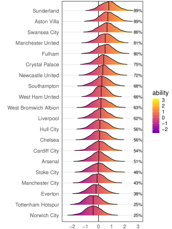
(b)

Figure 7: Posterior distribution of $\phi_{\textsf{Home\_Win}\to\textsf{Home\_Pass\_S}\mid 2}$ + $\omega_{c,\textsf{Home\_Pass\_S}}$ - $\phi_{\textsf{Away\_Win}\to\textsf{Away\_Pass\_S}\mid 2}$ - $\omega_{c,\textsf{Away\_Pass\_S}}$ in (a) and $\phi_{\textsf{Home\_Pass\_S}\to\textsf{Home\_Pass\_S}\mid 2}$ + $\omega_{c,\textsf{Home\_Pass\_S}}$ - $\phi_{\textsf{Away\_Pass\_S}\to\textsf{Away\_Pass\_S}\mid 2}$ - $\omega_{c,\textsf{Away\_Pass\_S}}$ in (b), from the baseline logit specification for incorporating team abilities in (13). Interpreted as the relative ability of a team to convert a Win to a Successful Pass when playing at home compared to away in (a) and similarly from one Successful Pass to another Successful Pass in (b). Teams are ranked in the decreasing order of the means of their respective posterior distributions shown by the overlaid vertical lines.

We also observe that the successful Pass events account for the majority of the background probability mass, while events like Shots and Goals have nearly zero probability. This suggests that the Shot and Goal events are highly unlikely to originate solely from the background component, but are instead triggered by excitations from previous events.

6.4 Excitation factor

The excitation factor $\alpha$ in expression (12) is a scaling factor applied to the contributions from the previous occurrences to the event mark probability. In (12), the background component has a weight of 1, while previous occurrences are weighted by $\exp(\alpha)$.

The 95% highest posterior density interval for $\exp(\alpha)$ is $(451.35,642.54)$, providing evidence that the contributions from previous occurrences carry substantially higher weight relative to the background component. In other words, this indicates that event sequences in football have a significant dependence on their history.

6.5 Decay rates

As mentioned in Section 4.2 the decay rate $\beta_{m\to m^{\prime}\mid z}$ in expression (12) is the exponential decay rate of the excitation caused by an event of mark $m$ on an event of mark $m^{\prime}$ at location $z$. By allowing the decay rates to depend on the pair of marks involved in the excitation, we had hoped to account for scenarios like a Corner event exciting a Pass_S event in the short term and a Shot event in the longer term. Indeed, the 95% highest posterior density interval for $\beta_{\textsf{Home\_Corner}\to\textsf{Home\_Pass\_S}\mid 3}$ is $(1.34,2.36)$ and $\beta_{\textsf{Home\_Corner}\to\textsf{Home\_Shot}\mid 3}$ is $(0.16,0.44)$ illustrating that the $\textsf{Corner}\to\textsf{Shot}$ excitation decays at a much slower rate compared to the $\textsf{Corner}\to\textsf{Pass\_S}$ excitation.

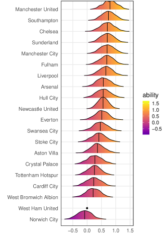
(a)

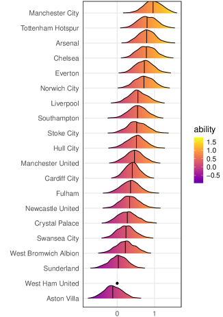
(b)

Figure 8: Posterior distribution of the parameters $\omega_{c,\textsf{Home\_Pass\_S}}$ in (a) and $\omega_{c,\textsf{Away\_Pass\_S}}$ in (b), from the baseline logit specification for incorporating team abilities in expression (13). Teams are ranked in the decreasing order of the means of their respective posterior distributions shown by the overlaid vertical lines.

6.6 Conversion rates

The parameter $\gamma_{m\to m^{\prime}\mid z}$ in expression (12) is the probability the excitation from an event of mark $m$ triggers an event of mark $m^{\prime}$ at location $z$.

Table 9 gives the posterior means and standard deviations of $\gamma_{m\to m^{\prime}\mid z}$ in the midfield region ($z=2$) for Manchester United. The probabilities for the $\textsf{Home\_Win}\to\textsf{Home\_Pass\_S}$, $\textsf{Home\_Dribble}\to\textsf{Home\_Pass\_S}$ and $\textsf{Home\_Pass\_S}\to\textsf{Home\_Pass\_S}$ conversions are higher compared to their away team counterparts, indicating that Manchester United is better in retaining possession of the ball when playing at home compared to away.

Figure 7 provides a ridge-line plot of the log odds ratio for home versus away ability of a team to convert a $\textsf{ Win}\to\textsf{ Pass\_S}$ (Figure 7(a)) and $\textsf{Pass\_S}\to\textsf{ Pass\_S}$ (Figure 7(b)). The teams are listed in decreasing order of the means of their respective posterior log odds ratios which are indicated by vertical lines. The percentage values by each plot, indicate the fraction of the distribution greater than 0. All but two teams in (Figure 7(a)) and five teams in (Figure 7(b)) have greater than $50\%$ of their distribution greater than 0, confirming that the vast majority of teams possess a higher ability to retain possession while playing at home.

In this way, we not only confirm the well-known home advantage effect, but also quantify team performance for games played at home as well as away.

6.7 Team abilities

Figure 8 provides a ridge-line plot of the posterior distribution of the parameters $\omega_{c,\textsf{Home\_Pass\_S}}$ and $\omega_{c,\textsf{Away\_Pass\_S}}$. The teams are listed in the decreasing order of the means of their respective posterior distributions which are indicated by vertical lines. We observe that Manchester United, the team with the highest ability to retain possession in home games (Figure 8(a)), drop significantly down in the rankings for the away games (Figure 8(b)). This is evidence that when Manchester United plays away they seem to deviate from the possession-based strategy they seem to adopt in the home games.

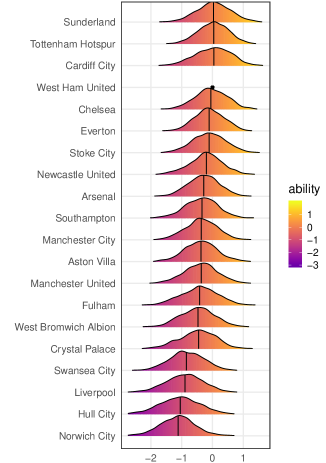
(a)

Team	Shots	Passes	S/P
Cardiff City	18	115	0.16
Sunderland	28	195	0.14
Tottenham Hotspur	37	261	0.14
Aston Villa	20	153	0.13
Newcastle United	22	180	0.12
Crystal Palace	18	148	0.12
Stoke City	24	199	0.12
Everton	40	342	0.12
Chelsea	29	248	0.12
Fulham	19	163	0.12
West Ham United	22	194	0.11
West Bromwich Albion	18	159	0.11
Swansea City	23	214	0.11
Arsenal	30	280	0.11
Southampton	23	223	0.10
Liverpool	28	292	0.10
Manchester United	22	238	0.09
Manchester City	30	330	0.09
Norwich City	19	227	0.08
Hull City	13	191	0.07

(b)

Figure 9: (a) Posterior distribution of $\omega_{c,\textsf{Home\_Shot}}+\omega_{c,\textsf{Away\_Shot}}$, the cumulative ability of a team $c$, relative to West Ham (baseline), to attempt a shot on goal. (b) The number of shots, passes completed in the attacking third and shots per pass completed in the attacking third (S/P) for each team in the training data.

Figure 9(a) provides a ridge-line plot of the posterior distribution of the cumulative ability of a team to attempt a shot on goal. A higher $\omega_{c,\textsf{Home\_Shot}}$, for example, indicates that for the team $c$, an event like Home_Pass_S is more likely to trigger a Home_Shot. We do not expect the cumulative abilities $\omega_{c,\textsf{Home\_Shot}}+\omega_{c,\textsf{Away\_Shot}}$ of the dominant teams to be high, as they might prefer to make additional passes to create better goal scoring opportunities. A weaker team, on the other hand, typically has fewer opportunities to attack and therefore, is more likely to attempt a shot on goal when possible. Indeed, this is what we observe in Figure 9, where we compare the team rankings based on their cumulative ability $\omega_{c,\textsf{Home\_Shot}}+\omega_{c,\textsf{Away\_Shot}}$ with the number of shots per pass completed in the attacking third (S/P column in Figure 9(b)) in the training data. The comparison between Cardiff City and Norwich City is an interesting example of two teams that appear to be similar with 18 and 19 shots on goal attempted, respectively, in their two games in the training data. However, the two teams are at the opposite ends of the ranking based on their cumulative ability $\omega_{c,\textsf{Home\_Shot}}+\omega_{c,\textsf{Away\_Shot}}$, capturing the clear difference between their attacking styles.

Table 10: (a) Team rankings based on the cumulative ability to trigger a particular event type. For example, the column Pass ranks teams in the decreasing order of their posterior means of $\omega_{c,\textsf{Home\_Pass\_S}}+\omega_{c,\textsf{Away\_Pass\_S}}$. The teams are ordered in (a) by the rankings based on their passing ability, which is a good indicator of the final position in the league table of the 2013/14 season in (b).

(a)

Team	Pass	Shot	Goal	Win	Save
Manchester City	1	11	1	15	11
Chelsea	2	5	11	20	4
Arsenal	3	9	3	5	7
Southampton	4	10	8	7	19
Manchester United	5	13	4	2	18
Everton	6	6	17	11	14
Liverpool	7	18	12	9	5
Hull City	8	19	15	1	10
Tottenham Hotspur	9	2	14	3	6
Fulham	10	14	7	14	3
Stoke City	11	7	9	12	8
Newcastle United	12	8	19	16	17
Sunderland	13	1	13	8	2
Swansea City	14	17	18	17	12
Cardiff City	15	3	2	19	15
Norwich City	16	20	10	4	20
Crystal Palace	17	16	16	13	16
West Bromwich Albion	18	15	20	10	1
Aston Villa	19	12	5	6	13
West Ham United	20	4	6	18	9

(b)

League Position	Team
1	Manchester City
2	Liverpool
3	Chelsea
4	Arsenal
5	Everton
6	Tottenham Hotspur
7	Manchester United
8	Southampton
9	Stoke City
10	Newcastle United
11	Crystal Palace
12	Swansea City
13	West Ham United
14	Sunderland
15	Aston Villa
16	Hull City
17	West Bromwich Albion
18	Norwich City
19	Fulham
20	Cardiff City

Table 10(a) shows the team rankings based on the cumulative ability to trigger five different event types. For example, the Pass column ranks teams in the decreasing order of their posterior means of $\omega_{c,\textsf{Home\_Pass\_S}}+\omega_{c,\textsf{Away\_Pass\_S}}$. The teams are ordered in Table 10(a) by the rankings based on their cumulative passing ability. Despite training on just the first 20 out of 380 games of the 2013/14 season, the rankings based on the passing ability is a good indicator of the positions the teams finished in the final league table of the 2013/14 season in Table 10(b).

6.8 Event genealogy

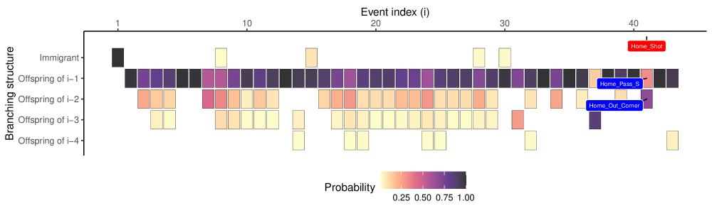
Figure 10: Posterior means of branching structure probabilities for events in the first 4 minutes of the game between Chelsea and Hull City on 18/08/2013. The highlighted event Home_Shot has a higher probability of being an offspring of the event Home_Out_Corner than being an offspring of the more recent Home_Pass_S event.

The branching structure $u_{si}$ indicates whether the $i$th event in $s$th sequence is an “immigrant” $(u_{si}=0)$ or an “offspring” of a previous event with index $j$ $(u_{si}=j)$. Given an observed event sequence $\mathcal{F}_{st_{sn_{s}}}$, the conditional branching structure probabilities $\mathbb{P}(u_{si}\mid\mathcal{F}_{st_{si}})$ based on the model specification in expression (12) are

$$\mathbb{P}(u_{si}=0\mid\mathcal{F}_{st_{si}}) =\frac{\delta_{m_{si}\mid z_{si}}}{\delta_{m_{si}\mid z_{si}}+\sum_{t_{sk}<t_{si}}\mathrm{e}^{\alpha-\beta_{m_{sk}\to m_{si}\mid z_{si}}(t_{si}-t_{sk})}\gamma_{m_{sk}\to m_{si}\mid z_{si}}}\,,$$

$$\mathbb{P}(u_{si}=j\mid\mathcal{F}_{st_{si}}) =\begin{cases}\frac{\mathrm{e}^{\alpha-\beta_{m_{sj}\to m_{si}\mid z_{si}}(t_{si}-t_{sj})}\gamma_{m_{sj}\to m_{si}\mid z_{si}}}{\delta_{m_{si}}+\sum_{t_{sk}<t_{si}}\mathrm{e}^{\alpha-\beta_{m_{sk}\to m_{si}\mid z_{si}}(t_{si}-t_{sk})}\gamma_{m_{sk}\to m_{si}\mid z_{si}}}&\text{for $t_{sj}<t_{si}$}\\ 0&\text{for $t_{sj}\geq t_{si}$}\end{cases}\,.$$ (17)

The branching structure probabilities in (17) quantify the relative contributions of the background process and previous occurrences in the mark probability of the $i$th event in the $s$th sequence. Figure 10 shows the posterior means of the branching structure probabilities for all events in the first four minutes of the game between Chelsea and Hull City on 18/08/2013. To illustrate the flexibility of the model to account for dependence between events over arbitrary durations of time, we highlight the event Home_Shot showing a higher probability of being an offspring of the event Home_Out_Corner than being an offspring of the more recent Home_Pass_S event.

7 Model-based predictions

Finally, we illustrate how the mechanistic modelling framework presented in this paper can be used to simulate event sequences in football and obtain predictions of event probabilities in real-time. We split the game between Arsenal and Tottenham Hotspur (01/09/2013) in the test data into 30-second intervals. For each interval, given the history of events up to but not including the interval, we simulate events over the next 30 seconds $Q=100$ times for each of the $R=500$ posterior samples from the M$\beta$A model with the tuning parameter setting ($W=5$, $N=100$).

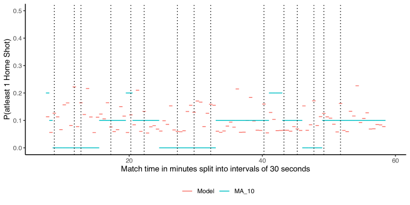
Figure 11: Forecasting the probability of observing at least one Home Shot event in 30-second intervals during the game between Arsenal and Tottenham Hotspur (01/09/2013) in the test data. Intervals with observed Home Shot events are highlighted using dotted lines. MA_10 is a 10-step moving average model used as a benchmark for comparison.

In Figure 11, we plot the proportion of all simulations within each interval where at least one Home_Shot event was simulated, and use dotted lines to denote the intervals where a Home_Shot event was actually observed. We also include a 10-step moving average model (MA_10) as a benchmark for comparison. We excluded the first 5 minutes of the game to ensure that we have predictions from both the models being compared. A quick inspection reveals that in 11 of the 15 intervals in which a Home_Shot is observed, the model predicts a shot probability greater than the 10-step moving average model.

In Figure 12, we formally validate the performance of the model against three moving average models for the classification task of whether a shot will be observed in an interval. For this purpose, we use data from the first 20 games in the test set, where we excluded the first 15 intervals of each game to ensure that we have predictions from all the four models being compared. To validate the models, we had a total of 1959 intervals out of which 202 intervals had at least one Home_Shot event. The area under the Receiver Operating Characteristic (ROC) curve is a performance measure that evaluates the performance of a classification model over all classification thresholds. The area under the curve (AUC) values are given in the legend and clearly confirm the superior performance of the model.

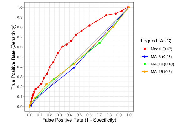
Figure 12: Validating the model performance against three moving average models for the task of whether a shot will be observed in each 30-second interval over the first 20 games in the test set. MA_5 is a 5-step moving average model and so on. The ROC curve evaluates the performance of a classification model over all classification thresholds. The area under the curve (AUC) values in the legend clearly confirm the superior performance of the model.

8 Discussion and concluding remarks

Building on the decomposition of a multivariate distribution function, we showed how the joint modelling in classical point process models like Hawkes processes, can be decoupled. The introduced flexible modelling framework can, for example, retain the characteristic property of excitation in Hawkes processes in the model for the marks while avoiding the clustering of event times. A comprehensive Bayesian approach for the modelling of flexible marked spatio-temporal point processes was developed including an approach to evaluate the predictive accuracy of the fitted Bayesian models using the out-of-sample log predictive density.

We presented a case study showing how the modelling framework developed in this paper can be tailored to separately model the components of the events in football, namely, the times, the locations and the event types. We were also able to incorporate team information into the model in a direct way that captured the relative abilities of the teams for each event type. We developed a method based on association rules to reduce the increased model complexity introduced by model extensions. The rule-based approach identified significant event interactions within sequences by placing thresholds on measures of significance. We then evaluated the accuracy of the excitation based models by comparing against two baseline models and confirmed the superior performance of the models with excitation effects.

We provided a detailed parameter description showing how the model parameters can be used to gain valuable insight into football. The excitation framework of the best performing model captured both the magnitudes and the durations of all pairwise event interactions across different locations. From the conversion rate parameters, we were able to quantify the well-known home advantage effect. We also discussed how the team ability parameters can be used to obtain rankings for the teams by event type, that can be used as predictors for team performance. The team ability parameters also captured some interesting differences in the playing styles of the teams, that were not immediately apparent just by looking at the data. In this way, the model along with its parameters can be used to develop a deeper understanding of the game-play by the coaching staff and inform strategic decision making. The proposed model can also be used to simulate the sequence of events in a game to obtain real-time predictions of event probabilities. We believe these predictions would enhance, among other aspects, the viewing experience of televised games.

The dataset we used consists of events from a single English Premier League season, which has a total of 380 games. However, as described in Section 6.1, we only used the first 20 games of the season as training data for the modelling exercise, over which every team in the league plays exactly one game each at Home and Away venues. This represents the minimum number of games required to ensure identifiability of all model parameters, specifically the team abilities. Even though the volume of data was kept to the minimum for computational reasons, our results illustrate that the model can provide valuable insights with limited data. So, the methodology developed in this paper can be readily applied to other team sports like rugby, hockey, basketball, American football etc where there may be fewer events per game or fewer games in a season.

Multiple seasons can be modelled together as if it were just one season using the modelling framework we propose, as long as the game rules, and hence, the definition of the events being considered does not change. Another aspect of the tournament to note is the relegation and promotion of teams within the league, which results in some teams not playing the same number of games over multiple seasons. A limitation of the proposed model is that the game periods are exchangeable, because the likelihood is invariant to the order in which the game periods and the games occur. It would be more natural to allow for the team ability parameters in (6) to be time-varying, especially over multiple seasons during which team players and managers are likely to change. Due to computational reasons we were not able to utilise most of the data even within a single season and current work focuses on overcoming this computational barrier using variational inference (Blei et al., 2017).

As none of the methods have been tailored specifically to football or even sports for that matter, they can be applied to a wide range of applications that generate event data streams. Specifically, the conversion rate parameters can be used to capture the triggering structure between different event types, for example, the probability of large earthquakes triggering smaller aftershocks. Also, the team ability parameters can be used for other multi-agent environments, for example, accidents by car type, countries in the analyses of financial events, individuals in identity systems, and so on.

9 Supporting materials

The raw data that motivated this work has been provided by Stratagem Technologies Ltd and consists of all touch-ball events for the 2013/14 season of the English Premier League. The raw data cannot be disclosed as the authors do not have the license to do so. The GitHub repository https://github.com/ForeStats/flexible-msttp-football provides all the computer code used for the data pre-processing and the Stan templates used to carry out the analyses presented in this paper. We also provide guidance on how the code can be used to apply our methods to similar data sets, like the publicly-available 2020/21 FA Women’s Super League Data provided by StatsBomb Inc. at https://github.com/statsbomb/open-data. Section S1 of the Supporting Materials document provides details on the prior distributions and the derivation of their posterior distributions for the FOMC and MSTHP models. Section S2 gives details on the association rule based screening procedure used to identify the most significant event interactions. We also provide the chain-wise trace plots for some of the parameters of the M$\beta$A model with $W=5$ and $N=100$.

10 Acknowledgements

The authors thank Stratagem Technologies Ltd for giving access to all touch-ball events from all English Premier League games in the 2013/14 season.

See pages - of supporting.pdf

References

- Agrawal et al. (1993) Agrawal, R., T. Imieliundefinedski, and A. Swami (1993). Mining association rules between sets of items in large databases. SIGMOD Rec. 22(2), 207–216.
- Agresti (2007) Agresti, A. (2007). An Introduction to Categorical Data Analysis (2nd ed.). Hoboken, NJ: Wiley.
- Blei et al. (2017) Blei, D. M., A. Kucukelbir, and J. D. McAuliffe (2017). Variational inference: A review for statisticians. Journal of the American statistical Association 112(518), 859–877.
- Borrie et al. (2002) Borrie, A., G. K. Jonsson, and M. S. Magnusson (2002). Temporal pattern analysis and its applicability in sport: an explanation and exemplar data. Journal of sports sciences 20(10), 845–852.
- Bowsher (2007) Bowsher, C. G. (2007). Modelling security market events in continuous time: Intensity based, multivariate point process models. Journal of Econometrics 141(2), 876–912.
- Clemente et al. (2015) Clemente, F. M., M. S. Couceiro, F. M. L. Martins, and R. S. Mendes (2015). Using network metrics in soccer: a macro-analysis. Journal of human kinetics 45(1), 123–134.
- Cox (1975) Cox, D. R. (1975). Partial likelihood. Biometrika 62(2), 269–276.
- Daley and Vere-Jones (2003) Daley, D. J. and D. Vere-Jones (2003). An introduction to the theory of point processes. Vol. I (2nd ed.). New York: Springer-Verlag.
- Decroos et al. (2018) Decroos, T., L. Bransen, J. Van Haaren, and J. Davis (2018). Actions Speak Louder Than Goals: Valuing Player Actions in Soccer. arXiv:1802.07127.
- Decroos et al. (2017) Decroos, T., V. Dzyuba, J. V. Haaren, and J. Davis (2017). Predicting soccer highlights from spatio-temporal match event streams. In S. P. Singh and S. Markovitch (Eds.), AAAI, pp. 1302–1308.
- Diggle (1985) Diggle, P. (1985). A kernel method for smoothing point process data. Journal of the Royal Statistical Society: Series C (Applied Statistics) 34(2), 138–147.
- Diggle (2013) Diggle, P. J. (2013). Statistical Analysis of Spatial and Spatio-Temporal Point Patterns (3rd ed.). Boca Raton, Florida: CRC Press.
- Duane et al. (1987) Duane, S., A. D. Kennedy, B. J. Pendleton, and D. Roweth (1987). Hybrid monte carlo. Physics letters B 195(2), 216–222.
- Duch et al. (2010) Duch, J., J. S. Waitzman, and L. A. N. Amaral (2010). Quantifying the performance of individual players in a team activity. PLOS One 5(6), e10937+.
- Gelman et al. (2013) Gelman, A., J. Carlin, H. Stern, D. Dunson, A. Vehtari, and D. Rubin (2013). Bayesian Data Analysis (3rd ed.). Boca Raton, Florida: CRC Press.
- Gelman et al. (1992) Gelman, A., D. B. Rubin, et al. (1992). Inference from iterative simulation using multiple sequences. Statistical science 7(4), 457–472.
- González et al. (2016) González, J. A., F. J. Rodríguez-Cortés, O. Cronie, and J. Mateu (2016). Spatio-temporal point process statistics: a review. Spatial Statistics 18, 505–544.
- Grund (2012) Grund, T. U. (2012). Network structure and team performance: The case of english premier league soccer teams. Social Networks 34(4), 682–690.
- Gudmundsson and Horton (2017) Gudmundsson, J. and M. Horton (2017). Spatio-temporal analysis of team sports. ACM Computing Surveys (CSUR) 50(2), 1–21.
- Hawkes (1971) Hawkes, A. G. (1971). Spectra of some self-exciting and mutually exciting point processes. Biometrika 58(1), 83–90.
- Hawkes and Oakes (1974) Hawkes, A. G. and D. Oakes (1974). A cluster process representation of a self-exciting process. Journal of Applied Probability 11(03), 493–503.
- Hoffman and Gelman (2014) Hoffman, M. D. and A. Gelman (2014). The no-u-turn sampler: Adaptively setting path lengths in hamiltonian monte carlo. Journal of Machine Learning Research 15(1), 1593–1623.
- Lindqvist (2006) Lindqvist, B. H. (2006). On the statistical modeling and analysis of repairable systems. Statistical Science 21(4), 532–551.
- Mackay (2017) Mackay, N. (2017). Predicting goal probabilities for possessions in football. Master’s thesis, Vrije Universiteit Amsterdam.
- Mohler et al. (2011) Mohler, G. O., M. B. Short, P. J. Brantingham, F. P. Schoenberg, and G. E. Tita (2011). Self-exciting point process modeling of crime. Journal of the American Statistical Association 106(493), 100–108.
- Narayanan (2021) Narayanan, S. (2021). Bayesian Modelling of Flexible Marked Point Processes with Applications to Event Sequences from Association Football. Ph. D. thesis, University of Warwick, Coventry. http://webcat.warwick.ac.uk/record=b3520069S̃15.
- Norris (1997) Norris, J. R. (1997). Markov Chains. Cambridge: Cambridge University Press.
- Ogata (1998) Ogata, Y. (1998). Space-time point-process models for earthquake occurrences. Annals of the Institute of Statistical Mathematics 50(2), 379–402.
- Passos et al. (2011) Passos, P., K. Davids, D. Araújo, N. Paz, J. Minguéns, and J. Mendes (2011). Networks as a novel tool for studying team ball sports as complex social systems. Journal of Science and Medicine in Sport 14(2), 170–176.
- Pena and Touchette (2012) Pena, J. L. and H. Touchette (2012). A network theory analysis of football strategies. arXiv:1206.6904.
- Rasmussen (2013) Rasmussen, J. G. (2013). Bayesian inference for hawkes processes. Methodology and Computing in Applied Probability 15(3), 623–642.
- Ripley (1977) Ripley, B. D. (1977). Modelling spatial patterns. Journal of the Royal Statistical Society: Series B (Methodological) 39(2), 172–192.
- Robberechts et al. (2019) Robberechts, P., J. Van Haaren, and J. Davis (2019). Who will win it? an in-game win probability model for football. arXiv:1906.05029.
- Routley and Schulte (2015) Routley, K. and O. Schulte (2015). A markov game model for valuing player actions in ice hockey. In M. Meila and T. Heskes (Eds.), UAI, pp. 782–791.
- Stan Development Team (2020) Stan Development Team (2020). Cmdstan: the command-line interface to stan. Version 2.22.1.
- Van Haaren et al. (2016) Van Haaren, J., S. Hannosset, and J. Davis (2016). Strategy discovery in professional soccer match data. In Proceedings of the KDD-16 Workshop on Large-Scale Sports Analytics, pp. 1–4.
- Veen and Schoenberg (2008) Veen, A. and F. P. Schoenberg (2008). Estimation of space–time branching process models in seismology using an em–type algorithm. Journal of the American Statistical Association 103(482), 614–624.
- Vehtari et al. (2017) Vehtari, A., A. Gelman, and J. Gabry (2017). Practical bayesian model evaluation using leave-one-out cross-validation and waic. Statistics and computing 27(5), 1413–1432.
- Vehtari et al. (2021) Vehtari, A., A. Gelman, D. Simpson, B. Carpenter, and P.-C. Bürkner (2021). Rank-Normalization, Folding, and Localization: An Improved for Assessing Convergence of MCMC (with Discussion). Bayesian Analysis 16(2), 667–718.
- Wang et al. (2015) Wang, Q., H. Zhu, W. Hu, Z. Shen, and Y. Yao (2015). Discerning tactical patterns for professional soccer teams: an enhanced topic model with applications. In Proceedings of the 21th ACM SIGKDD International Conference on Knowledge Discovery and Data Mining, pp. 2197–2206.