Key words:
Growth-collapse processes,
Poisson shot noise,
uniform cut-off,
stochastic integrals with jumps,
moments,
cumulants.
1 Introduction
Markovian growth-collapse processes, see Eliazar and Klafter ( 2004 ) Davis ( 1984 ) Frolkova and Mandjes ( 2019 )
The computation of moments of growth-collapse processes has been
the object of several approaches, see
Boxma et al. ( 2006 ) Daw and Pender ( 2020 )
In this paper,
we apply general moment identities
written as sums over partitions
for Poisson stochastic integrals with
random integrands, see Privault ( 2012a b ; 2009 2016 )
Let ( N t ) t ∈ + subscript subscript 𝑁 𝑡 subscript 𝑡 absent (N_{t})_{t\in_{+}} λ 𝜆 \lambda + , and
consider a process ( Y t ) t ∈ + subscript subscript 𝑌 𝑡 subscript 𝑡 absent (Y_{t})_{t\in_{+}}
Y t = ∫ 0 t f ( N s − ) 𝑑 N s , t ≥ 0 . formulae-sequence subscript 𝑌 𝑡 superscript subscript 0 𝑡 𝑓 subscript 𝑁 superscript 𝑠 differential-d subscript 𝑁 𝑠 𝑡 0 Y_{t}=\int_{0}^{t}f(N_{s^{-}})dN_{s},\qquad t\geq 0.
As the left limit f ( N s − ) 𝑓 subscript 𝑁 superscript 𝑠 f(N_{s^{-}}) ( ℱ s ) s ∈ + subscript subscript ℱ 𝑠 subscript 𝑠 absent ({\cal F}_{s})_{s\in_{+}} ( N s ) s ∈ + subscript subscript 𝑁 𝑠 subscript 𝑠 absent (N_{s})_{s\in_{+}} Y t subscript 𝑌 𝑡 Y_{t} Brémaud ( 1999 )
𝔼 [ Y t ] = λ 𝔼 [ ∫ 0 t f ( N s − ) 𝑑 s ] = λ ∫ 0 t 𝔼 [ f ( N s − ) ] 𝑑 s , t ≥ 0 . formulae-sequence 𝔼 delimited-[] subscript 𝑌 𝑡 𝜆 𝔼 delimited-[] superscript subscript 0 𝑡 𝑓 subscript 𝑁 superscript 𝑠 differential-d 𝑠 𝜆 superscript subscript 0 𝑡 𝔼 delimited-[] 𝑓 subscript 𝑁 superscript 𝑠 differential-d 𝑠 𝑡 0 \mathbb{E}[Y_{t}]=\lambda\mathbb{E}\left[\int_{0}^{t}f(N_{s^{-}})ds\right]=\lambda\int_{0}^{t}\mathbb{E}\left[f(N_{s^{-}})\right]ds,\qquad t\geq 0.
This calculation does not apply however to the process
f ( N s ) 𝑓 subscript 𝑁 𝑠 f(N_{s}) ( ℱ s ) s ∈ + subscript subscript ℱ 𝑠 subscript 𝑠 absent ({\cal F}_{s})_{s\in_{+}} Slivnyak ( 1962 ) Mecke ( 1967 )
𝔼 [ Y t ] = λ 𝔼 [ ∫ 0 t ε s + f ( N s ) 𝑑 s ] = λ 𝔼 [ ∫ 0 t f ( 1 + N s ) 𝑑 s ] , t ≥ 0 , formulae-sequence 𝔼 delimited-[] subscript 𝑌 𝑡 𝜆 𝔼 delimited-[] superscript subscript 0 𝑡 subscript superscript 𝜀 𝑠 𝑓 subscript 𝑁 𝑠 differential-d 𝑠 𝜆 𝔼 delimited-[] superscript subscript 0 𝑡 𝑓 1 subscript 𝑁 𝑠 differential-d 𝑠 𝑡 0 \mathbb{E}[Y_{t}]=\lambda\mathbb{E}\left[\int_{0}^{t}\varepsilon^{+}_{s}f(N_{s})ds\right]=\lambda\mathbb{E}\left[\int_{0}^{t}f(1+N_{s})ds\right],\qquad t\geq 0,
where ε s + subscript superscript 𝜀 𝑠 \varepsilon^{+}_{s} s ≥ 0 𝑠 0 s\geq 0
In order to compute higher order moments we will
apply a nonlinear extension of the
Slivnyak-Mecke identity, see Proposition 2.1 3
Y t = ∑ k = 1 N t g ( T k , k , N t ) = ∫ 0 t g ( s , N s , N t ) 𝑑 N s , subscript 𝑌 𝑡 superscript subscript 𝑘 1 subscript 𝑁 𝑡 𝑔 subscript 𝑇 𝑘 𝑘 subscript 𝑁 𝑡 superscript subscript 0 𝑡 𝑔 𝑠 subscript 𝑁 𝑠 subscript 𝑁 𝑡 differential-d subscript 𝑁 𝑠 Y_{t}=\sum_{k=1}^{N_{t}}g(T_{k},k,N_{t})=\int_{0}^{t}g(s,N_{s},N_{t})dN_{s},
where ( T k ) k ≥ 1 subscript subscript 𝑇 𝑘 𝑘 1 (T_{k})_{k\geq 1} ( N t ) t ∈ + subscript subscript 𝑁 𝑡 subscript 𝑡 absent (N_{t})_{t\in_{+}} 3.1 3.2 4
Y t = ∑ k = 1 N t f k ( T k ) ( 1 − U k ) ∏ l = k + 1 N t U l , t ∈ + , Y_{t}=\sum_{k=1}^{N_{t}}f_{k}(T_{k})(1-U_{k})\prod_{l=k+1}^{N_{t}}U_{l},\qquad t\in_{+},
where ( U k ) k ≥ 1 subscript subscript 𝑈 𝑘 𝑘 1 (U_{k})_{k\geq 1} [ 0 , 1 ] 0 1 [0,1] ( N t ) t ∈ + subscript subscript 𝑁 𝑡 subscript 𝑡 absent (N_{t})_{t\in_{+}} 4.1
In particular, in Proposition 5.1
𝔼 [ ( X t ) n ] = ( n + 1 ) ! λ n ∑ k = 0 n ( − 1 ) k ( k + 1 ) n − 1 ( n k ) e − k λ t / ( k + 1 ) , t ∈ + , \mathbb{E}[(X_{t})^{n}]=\frac{(n+1)!}{\lambda^{n}}\sum_{k=0}^{n}(-1)^{k}(k+1)^{n-1}{n\choose k}\mathrm{e}^{-k\lambda t/(k+1)},\qquad t\in_{+}, (1.1)
for the moments of all orders n ≥ 0 𝑛 0 n\geq 0
X t = t − ∑ k = 1 N t T k ( 1 − U k ) ∏ l = k + 1 N t U l , t ∈ + , X_{t}=t-\sum_{k=1}^{N_{t}}T_{k}(1-U_{k})\prod_{l=k+1}^{N_{t}}U_{l},\qquad t\in_{+},
where ( U k ) k ≥ 1 subscript subscript 𝑈 𝑘 𝑘 1 (U_{k})_{k\geq 1} [ 0 , 1 ] 0 1 [0,1] Boxma et al. ( 2006 ) Daw and Pender ( 2020 ) 1.1
lim t → ∞ 𝔼 [ ( X t ) n ] = ( n + 1 ) ! λ n , n ≥ 1 , formulae-sequence subscript → 𝑡 𝔼 delimited-[] superscript subscript 𝑋 𝑡 𝑛 𝑛 1 superscript 𝜆 𝑛 𝑛 1 \lim_{t\to\infty}\mathbb{E}[(X_{t})^{n}]=\frac{(n+1)!}{\lambda^{n}},\qquad n\geq 1,
which recover
the gamma stationary distribution of ( X t ) t ∈ + subscript subscript 𝑋 𝑡 subscript 𝑡 absent (X_{t})_{t\in_{+}} 2 2 2 Boxma et al. ( 2006 )
Finally, in Section 6
Y ( m ) = ∑ k = 1 m g ( T k , k , m ) = ∫ 0 T m g ( s , N s , m ) 𝑑 N s , m ≥ 1 , formulae-sequence 𝑌 𝑚 superscript subscript 𝑘 1 𝑚 𝑔 subscript 𝑇 𝑘 𝑘 𝑚 superscript subscript 0 subscript 𝑇 𝑚 𝑔 𝑠 subscript 𝑁 𝑠 𝑚 differential-d subscript 𝑁 𝑠 𝑚 1 Y(m)=\sum_{k=1}^{m}g(T_{k},k,m)=\int_{0}^{T_{m}}g(s,N_{s},m)dN_{s},\qquad m\geq 1,
see Corollaries 6.2 6.3
X ( m ) = T m − ∑ k = 1 m T k ( 1 − U k ) ∏ l = k + 1 m U l , m ≥ 1 , formulae-sequence 𝑋 𝑚 subscript 𝑇 𝑚 superscript subscript 𝑘 1 𝑚 subscript 𝑇 𝑘 1 subscript 𝑈 𝑘 superscript subscript product 𝑙 𝑘 1 𝑚 subscript 𝑈 𝑙 𝑚 1 X(m)=T_{m}-\sum_{k=1}^{m}T_{k}(1-U_{k})\prod_{l=k+1}^{m}U_{l},\qquad m\geq 1,
where ( U k ) k ≥ 1 subscript subscript 𝑈 𝑘 𝑘 1 (U_{k})_{k\geq 1} [ 0 , 1 ] 0 1 [0,1] 6.4 6.5 Boxma et al. ( 2006 )
We proceed as follows.
In Section 2 3 4 5 6
2 Moment identities for Poisson stochastic integrals
In this section we review the computation of moments of
Poisson stochastic integrals with random integrands using sums over partitions,
see Proposition 3.1 in Privault ( 2012a ) ( N t ) t ∈ + subscript subscript 𝑁 𝑡 subscript 𝑡 absent (N_{t})_{t\in_{+}} N t = ω ( [ 0 , t ] ) subscript 𝑁 𝑡 𝜔 0 𝑡 N_{t}=\omega([0,t]) ω ( d s ) 𝜔 𝑑 𝑠 \omega(ds) λ ( d s ) 𝜆 𝑑 𝑠 \lambda(ds) ( T k ) k ≥ 1 subscript subscript 𝑇 𝑘 𝑘 1 (T_{k})_{k\geq 1} s 1 , … , s k ∈ + subscript subscript 𝑠 1 … subscript 𝑠 𝑘
absent s_{1},\ldots,s_{k}\in_{+} ϵ s 1 + ⋯ ϵ s k + subscript superscript italic-ϵ subscript 𝑠 1 ⋯ subscript superscript italic-ϵ subscript 𝑠 𝑘 \epsilon^{+}_{s_{1}}\cdots\epsilon^{+}_{s_{k}}
( ϵ s 1 + ⋯ ϵ s k + F ) ( ω ) = F ( ω ∪ { s 1 , … , s k } ) subscript superscript italic-ϵ subscript 𝑠 1 ⋯ subscript superscript italic-ϵ subscript 𝑠 𝑘 𝐹 𝜔 𝐹 𝜔 subscript 𝑠 1 … subscript 𝑠 𝑘 (\epsilon^{+}_{s_{1}}\cdots\epsilon^{+}_{s_{k}}F)(\omega)=F(\omega\cup\{s_{1},\ldots,s_{k}\})
acting on random variables F 𝐹 F s 1 , … , s k subscript 𝑠 1 … subscript 𝑠 𝑘
s_{1},\ldots,s_{k} ω ( d x ) 𝜔 𝑑 𝑥 \omega(dx) F 𝐹 F F = f ( N t 1 , … , N t n ) 𝐹 𝑓 subscript 𝑁 subscript 𝑡 1 … subscript 𝑁 subscript 𝑡 𝑛 F=f(N_{t_{1}},\ldots,N_{t_{n}})
ϵ s 1 + ⋯ ϵ s k + F = f ( N t 1 + # { k : s k ≤ t 1 } , … , N t n + # { k : s k ≤ t n } ) . subscript superscript italic-ϵ subscript 𝑠 1 ⋯ subscript superscript italic-ϵ subscript 𝑠 𝑘 𝐹 𝑓 subscript 𝑁 subscript 𝑡 1 # conditional-set 𝑘 subscript 𝑠 𝑘 subscript 𝑡 1 … subscript 𝑁 subscript 𝑡 𝑛 # conditional-set 𝑘 subscript 𝑠 𝑘 subscript 𝑡 𝑛 \epsilon^{+}_{s_{1}}\cdots\epsilon^{+}_{s_{k}}F=f(N_{t_{1}}+\#\{k\ :\ s_{k}\leq t_{1}\},\ldots,N_{t_{n}}+\#\{k\ :\ s_{k}\leq t_{n}\}).
The following moment identity, see Proposition 3.1 in Privault ( 2012a ) Privault ( 2016 ) { π 1 , … , π k } subscript 𝜋 1 … subscript 𝜋 𝑘 \{\pi_{1},\ldots,\pi_{k}\} { 1 , … , n } 1 … 𝑛 \{1,\ldots,n\} u : + × Ω ⟶ u:_{+}\times\Omega\longrightarrow
Proposition 2.1
Let ( u s ( ω ) ) s ∈ + subscript subscript 𝑢 𝑠 𝜔 subscript 𝑠 absent (u_{s}(\omega))_{s\in_{+}} s ∈ + subscript 𝑠 absent s\in_{+} n ≥ 1 𝑛 1 n\geq 1
𝔼 [ ( ∫ 0 T u s 𝑑 N s ) n ] 𝔼 delimited-[] superscript superscript subscript 0 𝑇 subscript 𝑢 𝑠 differential-d subscript 𝑁 𝑠 𝑛 \displaystyle\mathbb{E}\left[\left(\int_{0}^{T}u_{s}dN_{s}\right)^{n}\right] (2.1)
= ∑ k = 1 n ∑ π 1 ∪ ⋯ ∪ π k = { 1 , … , n } 𝔼 [ ∫ 0 t ⋯ ∫ 0 t ϵ s 1 + ⋯ ϵ s k + ( u | π 1 | ( s 1 , ω ) ⋯ u | π k | ( s k , ω ) ) λ ( d s 1 ) ⋯ λ ( d s k ) ] , absent superscript subscript 𝑘 1 𝑛 subscript subscript 𝜋 1 ⋯ subscript 𝜋 𝑘 1 … 𝑛 𝔼 delimited-[] superscript subscript 0 𝑡 ⋯ superscript subscript 0 𝑡 subscript superscript italic-ϵ subscript 𝑠 1 ⋯ subscript superscript italic-ϵ subscript 𝑠 𝑘 superscript 𝑢 subscript 𝜋 1 subscript 𝑠 1 𝜔 ⋯ superscript 𝑢 subscript 𝜋 𝑘 subscript 𝑠 𝑘 𝜔 𝜆 𝑑 subscript 𝑠 1 ⋯ 𝜆 𝑑 subscript 𝑠 𝑘 \displaystyle=\sum_{k=1}^{n}\sum_{\pi_{1}\cup\cdots\cup\pi_{k}=\{1,\ldots,n\}}\mathbb{E}\left[\int_{0}^{t}\cdots\int_{0}^{t}\epsilon^{+}_{s_{1}}\cdots\epsilon^{+}_{s_{k}}\big{(}u^{|\pi_{1}|}(s_{1},\omega)\cdots u^{|\pi_{k}|}(s_{k},\omega)\big{)}\lambda(ds_{1})\cdots\lambda(ds_{k})\right],
where the power | π i | subscript 𝜋 𝑖 |\pi_{i}| π i subscript 𝜋 𝑖 \pi_{i} π 1 , … , π k subscript 𝜋 1 … subscript 𝜋 𝑘
\pi_{1},\ldots,\pi_{k} { 1 , … , n } 1 … 𝑛 \{1,\ldots,n\}
In the sequel we will frequently use the equivalent
combinatorial expressions
∑ k = 1 n ∑ π 1 ∪ … ∪ π k = { 1 , … , n } f k ( | π 1 | , … , | π k | ) superscript subscript 𝑘 1 𝑛 subscript subscript 𝜋 1 … subscript 𝜋 𝑘 1 … 𝑛 subscript 𝑓 𝑘 subscript 𝜋 1 … subscript 𝜋 𝑘 \displaystyle\sum_{k=1}^{n}\sum_{\pi_{1}\cup\ldots\cup\pi_{k}=\{1,\ldots,n\}}f_{k}(|\pi_{1}|,\ldots,|\pi_{k}|) = \displaystyle= ∑ k = 1 n n ! k ! ∑ p 1 + ⋯ + p k = n p 1 , … , p k ≥ 1 f k ( p 1 , … , p k ) p 1 ! ⋯ p k ! superscript subscript 𝑘 1 𝑛 𝑛 𝑘 subscript FRACOP subscript 𝑝 1 ⋯ subscript 𝑝 𝑘 𝑛 subscript 𝑝 1 … subscript 𝑝 𝑘
1 subscript 𝑓 𝑘 subscript 𝑝 1 … subscript 𝑝 𝑘 subscript 𝑝 1 ⋯ subscript 𝑝 𝑘 \displaystyle\sum_{k=1}^{n}\frac{n!}{k!}\sum_{p_{1}+\cdots+p_{k}=n\atop p_{1},\ldots,p_{k}\geq 1}\frac{f_{k}(p_{1},\ldots,p_{k})}{p_{1}!\cdots p_{k}!}
= \displaystyle= ∑ k = 1 n n ! k ! ∑ q 0 = 0 < q 1 < ⋯ < q k = n f k ( q 1 − q 0 , … , q k − q k − 1 ) ( q 1 − q 0 ) ! ⋯ ( q k − q k − 1 ) ! superscript subscript 𝑘 1 𝑛 𝑛 𝑘 subscript subscript 𝑞 0 0 subscript 𝑞 1 ⋯ subscript 𝑞 𝑘 𝑛 subscript 𝑓 𝑘 subscript 𝑞 1 subscript 𝑞 0 … subscript 𝑞 𝑘 subscript 𝑞 𝑘 1 subscript 𝑞 1 subscript 𝑞 0 ⋯ subscript 𝑞 𝑘 subscript 𝑞 𝑘 1 \displaystyle\sum_{k=1}^{n}\frac{n!}{k!}\sum_{q_{0}=0<q_{1}<\cdots<q_{k}=n}\frac{f_{k}(q_{1}-q_{0},\ldots,q_{k}-q_{k-1})}{(q_{1}-q_{0})!\cdots(q_{k}-q_{k-1})!}
for f k subscript 𝑓 𝑘 f_{k} ℕ k superscript ℕ 𝑘 {\mathord{\mathbb{N}}}^{k} k = 1 , … , n 𝑘 1 … 𝑛
k=1,\ldots,n x 1 , … , x n ∈ subscript 𝑥 1 … subscript 𝑥 𝑛
absent x_{1},\ldots,x_{n}\in f k ( p 1 , … , p k ) = x p 1 ⋯ x p k subscript 𝑓 𝑘 subscript 𝑝 1 … subscript 𝑝 𝑘 subscript 𝑥 subscript 𝑝 1 ⋯ subscript 𝑥 subscript 𝑝 𝑘 f_{k}(p_{1},\ldots,p_{k})=x_{p_{1}}\cdots x_{p_{k}} n ≥ 1 𝑛 1 n\geq 1
B n ( x 1 , … , x n ) subscript 𝐵 𝑛 subscript 𝑥 1 … subscript 𝑥 𝑛 \displaystyle B_{n}(x_{1},\ldots,x_{n}) = \displaystyle= ∑ k = 1 n n ! k ! ∑ p 1 + ⋯ + p k = n p 1 ≥ 1 , … , p k ≥ 1 x p 1 ⋯ x p k p 1 ! ⋯ p k ! superscript subscript 𝑘 1 𝑛 𝑛 𝑘 subscript FRACOP subscript 𝑝 1 ⋯ subscript 𝑝 𝑘 𝑛 formulae-sequence subscript 𝑝 1 1 …
subscript 𝑝 𝑘 1 subscript 𝑥 subscript 𝑝 1 ⋯ subscript 𝑥 subscript 𝑝 𝑘 subscript 𝑝 1 ⋯ subscript 𝑝 𝑘 \displaystyle\sum_{k=1}^{n}\frac{n!}{k!}\sum_{p_{1}+\cdots+p_{k}=n\atop p_{1}\geq 1,\ldots,p_{k}\geq 1}\frac{x_{p_{1}}\cdots x_{p_{k}}}{p_{1}!\cdots p_{k}!}
= \displaystyle= ∑ k = 0 n ∑ π 1 ∪ ⋯ ∪ π k = { 1 , … , n } x | π 1 | ⋯ x | π k | . superscript subscript 𝑘 0 𝑛 subscript subscript 𝜋 1 ⋯ subscript 𝜋 𝑘 1 … 𝑛 subscript 𝑥 subscript 𝜋 1 ⋯ subscript 𝑥 subscript 𝜋 𝑘 \displaystyle\sum_{k=0}^{n}~{}\sum_{\pi_{1}\cup\cdots\cup\pi_{k}=\{1,\ldots,n\}}x_{|\pi_{1}|}\cdots x_{|\pi_{k}|}.
We will also use the relation
𝔼 [ X n ] = B n ( κ X ( 1 ) , … , κ X ( n ) ) 𝔼 delimited-[] superscript 𝑋 𝑛 subscript 𝐵 𝑛 superscript subscript 𝜅 𝑋 1 … superscript subscript 𝜅 𝑋 𝑛 \mathbb{E}[X^{n}]=B_{n}(\kappa_{X}^{(1)},\ldots,\kappa_{X}^{(n)}) 𝔼 [ X n ] 𝔼 delimited-[] superscript 𝑋 𝑛 \mathbb{E}[X^{n}] κ X ( n ) superscript subscript 𝜅 𝑋 𝑛 \kappa_{X}^{(n)} X 𝑋 X
κ n X = ∑ k = 1 n ( k − 1 ) ! ( − 1 ) k − 1 ∑ π 1 ∪ ⋯ ∪ π k = { 1 , … , n } 𝔼 [ X | π 1 | ] ⋯ 𝔼 [ X | π k | ] , n ≥ 1 , formulae-sequence subscript superscript 𝜅 𝑋 𝑛 superscript subscript 𝑘 1 𝑛 𝑘 1 superscript 1 𝑘 1 subscript subscript 𝜋 1 ⋯ subscript 𝜋 𝑘 1 … 𝑛 𝔼 delimited-[] superscript 𝑋 subscript 𝜋 1 ⋯ 𝔼 delimited-[] superscript 𝑋 subscript 𝜋 𝑘 𝑛 1 \kappa^{X}_{n}=\sum_{k=1}^{n}(k-1)!(-1)^{k-1}\sum_{\pi_{1}\cup\cdots\cup\pi_{k}=\{1,\ldots,n\}}\mathbb{E}\big{[}X^{|\pi_{1}|}\big{]}\cdots\mathbb{E}\big{[}X^{|\pi_{k}|}\big{]},\qquad n\geq 1, (2.2)
see Theorem 1 of Lukacs ( 1955 ) Leonov and Shiryaev ( 1959 )
Shot noise processes
Before moving to the setting of Markovian growth-collapse processes,
we use the case of Poisson shot noise processes as an illustration for
the result of Proposition 2.1 ( S t ) t ∈ + subscript subscript 𝑆 𝑡 subscript 𝑡 absent (S_{t})_{t\in_{+}}
S t = ∑ k = 1 N t J k g ( T k , t ) = ∑ k = 1 N t J N T k g ( T k , t ) = ∫ 0 t J N s g ( s , t ) 𝑑 N s , t ∈ + , formulae-sequence subscript 𝑆 𝑡 superscript subscript 𝑘 1 subscript 𝑁 𝑡 subscript 𝐽 𝑘 𝑔 subscript 𝑇 𝑘 𝑡 superscript subscript 𝑘 1 subscript 𝑁 𝑡 subscript 𝐽 subscript 𝑁 subscript 𝑇 𝑘 𝑔 subscript 𝑇 𝑘 𝑡 superscript subscript 0 𝑡 subscript 𝐽 subscript 𝑁 𝑠 𝑔 𝑠 𝑡 differential-d subscript 𝑁 𝑠 subscript 𝑡 absent S_{t}=\sum_{k=1}^{N_{t}}J_{k}g(T_{k},t)=\sum_{k=1}^{N_{t}}J_{N_{T_{k}}}g(T_{k},t)=\int_{0}^{t}J_{N_{s}}g(s,t)dN_{s},\qquad t\in_{+},
where ( J k ) k ≥ 0 subscript subscript 𝐽 𝑘 𝑘 0 (J_{k})_{k\geq 0} g ( ⋅ , ⋅ ) 𝑔 ⋅ ⋅ g(\cdot,\cdot) Daw and Pender ( 2020 ) λ ( d s ) = λ d s 𝜆 𝑑 𝑠 𝜆 𝑑 𝑠 \lambda(ds)=\lambda ds λ > 0 𝜆 0 \lambda>0 g ( s , t ) = e − β ( t − s ) 𝑔 𝑠 𝑡 superscript e 𝛽 𝑡 𝑠 g(s,t)=\mathrm{e}^{-\beta(t-s)} β > 0 𝛽 0 \beta>0
Proposition 2.2
For any n ≥ 1 𝑛 1 n\geq 1
𝔼 [ S t n ] = B n ( 𝔼 [ J 1 ] ∫ 0 t g ( s , t ) 𝑑 s , … , 𝔼 [ J 1 n ] ∫ 0 t g n ( s , t ) 𝑑 s ) , 𝔼 delimited-[] superscript subscript 𝑆 𝑡 𝑛 subscript 𝐵 𝑛 𝔼 delimited-[] subscript 𝐽 1 superscript subscript 0 𝑡 𝑔 𝑠 𝑡 differential-d 𝑠 … 𝔼 delimited-[] superscript subscript 𝐽 1 𝑛 superscript subscript 0 𝑡 superscript 𝑔 𝑛 𝑠 𝑡 differential-d 𝑠 \mathbb{E}[S_{t}^{n}]=B_{n}\left(\mathbb{E}\big{[}J_{1}\big{]}\int_{0}^{t}g(s,t)ds,\ldots,\mathbb{E}\big{[}J_{1}^{n}\big{]}\int_{0}^{t}g^{n}(s,t)ds\right),
where B n subscript 𝐵 𝑛 B_{n} n ≥ 1 𝑛 1 n\geq 1
Proof.
Taking
u s ( ω ) := J N s g ( s , t ) assign subscript 𝑢 𝑠 𝜔 subscript 𝐽 subscript 𝑁 𝑠 𝑔 𝑠 𝑡 u_{s}(\omega):=J_{N_{s}}g(s,t) 2.1
𝔼 [ S t n ] = 𝔼 [ ( ∑ k = 1 N t J N T k g ( T k , t ) ) n ] 𝔼 delimited-[] superscript subscript 𝑆 𝑡 𝑛 𝔼 delimited-[] superscript superscript subscript 𝑘 1 subscript 𝑁 𝑡 subscript 𝐽 subscript 𝑁 subscript 𝑇 𝑘 𝑔 subscript 𝑇 𝑘 𝑡 𝑛 \displaystyle\mathbb{E}[S_{t}^{n}]=\mathbb{E}\left[\left(\sum_{k=1}^{N_{t}}J_{N_{T_{k}}}g(T_{k},t)\right)^{n}\right]
= 𝔼 [ ( ∑ k = 1 N t u T k ( ω ) ) n ] absent 𝔼 delimited-[] superscript superscript subscript 𝑘 1 subscript 𝑁 𝑡 subscript 𝑢 subscript 𝑇 𝑘 𝜔 𝑛 \displaystyle=\mathbb{E}\left[\left(\sum_{k=1}^{N_{t}}u_{T_{k}}(\omega)\right)^{n}\right]
= ∑ l = 1 n ∑ π 1 ∪ ⋯ ∪ π l = { 1 , … , n } 𝔼 [ ∫ 0 t ⋯ ∫ 0 t ϵ s 1 + ⋯ ϵ s l + ( u | π 1 | ( s 1 , ω ) ⋯ u | π l | ( s l , ω ) ) λ ( d s 1 ) ⋯ λ ( d s l ) ] absent superscript subscript 𝑙 1 𝑛 subscript subscript 𝜋 1 ⋯ subscript 𝜋 𝑙 1 … 𝑛 𝔼 delimited-[] superscript subscript 0 𝑡 ⋯ superscript subscript 0 𝑡 subscript superscript italic-ϵ subscript 𝑠 1 ⋯ subscript superscript italic-ϵ subscript 𝑠 𝑙 superscript 𝑢 subscript 𝜋 1 subscript 𝑠 1 𝜔 ⋯ superscript 𝑢 subscript 𝜋 𝑙 subscript 𝑠 𝑙 𝜔 𝜆 𝑑 subscript 𝑠 1 ⋯ 𝜆 𝑑 subscript 𝑠 𝑙 \displaystyle=\sum_{l=1}^{n}\sum_{\pi_{1}\cup\cdots\cup\pi_{l}=\{1,\ldots,n\}}\mathbb{E}\left[\int_{0}^{t}\cdots\int_{0}^{t}\epsilon^{+}_{s_{1}}\cdots\epsilon^{+}_{s_{l}}\big{(}u^{|\pi_{1}|}(s_{1},\omega)\cdots u^{|\pi_{l}|}(s_{l},\omega)\big{)}\lambda(ds_{1})\cdots\lambda(ds_{l})\right]
= ∑ l = 1 n ∑ π 1 ∪ ⋯ ∪ π l = { 1 , … , n } ∫ 0 t ⋯ ∫ 0 t g | π 1 | ( s 1 , t ) ⋯ g | π l | ( s l , t ) 𝔼 [ ϵ s 1 + ⋯ ϵ s l + ( J N s 1 | π 1 | ⋯ J N s l | π l | ) ] λ ( d s 1 ) ⋯ λ ( d s l ) absent superscript subscript 𝑙 1 𝑛 subscript subscript 𝜋 1 ⋯ subscript 𝜋 𝑙 1 … 𝑛 superscript subscript 0 𝑡 ⋯ superscript subscript 0 𝑡 superscript 𝑔 subscript 𝜋 1 subscript 𝑠 1 𝑡 ⋯ superscript 𝑔 subscript 𝜋 𝑙 subscript 𝑠 𝑙 𝑡 𝔼 delimited-[] subscript superscript italic-ϵ subscript 𝑠 1 ⋯ subscript superscript italic-ϵ subscript 𝑠 𝑙 superscript subscript 𝐽 subscript 𝑁 subscript 𝑠 1 subscript 𝜋 1 ⋯ superscript subscript 𝐽 subscript 𝑁 subscript 𝑠 𝑙 subscript 𝜋 𝑙 𝜆 𝑑 subscript 𝑠 1 ⋯ 𝜆 𝑑 subscript 𝑠 𝑙 \displaystyle=\sum_{l=1}^{n}\sum_{\pi_{1}\cup\cdots\cup\pi_{l}=\{1,\ldots,n\}}\int_{0}^{t}\cdots\int_{0}^{t}g^{|\pi_{1}|}(s_{1},t)\cdots g^{|\pi_{l}|}(s_{l},t)\mathbb{E}\big{[}\epsilon^{+}_{s_{1}}\cdots\epsilon^{+}_{s_{l}}\big{(}J_{N_{s_{1}}}^{|\pi_{1}|}\cdots J_{N_{s_{l}}}^{|\pi_{l}|}\big{)}\big{]}\lambda(ds_{1})\cdots\lambda(ds_{l})
= ∑ l = 1 n ∑ π 1 ∪ ⋯ ∪ π l = { 1 , … , n } ∫ 0 t ⋯ ∫ 0 t g | π 1 | ( s 1 , t ) ⋯ g | π l | ( s l , t ) 𝔼 [ J N s 1 | π 1 | ] 𝔼 [ J 1 + N s 1 | π 1 | ] ⋯ 𝔼 [ J l − 1 + N s l | π l | ] λ ( d s 1 ) ⋯ λ ( d s l ) absent superscript subscript 𝑙 1 𝑛 subscript subscript 𝜋 1 ⋯ subscript 𝜋 𝑙 1 … 𝑛 superscript subscript 0 𝑡 ⋯ superscript subscript 0 𝑡 superscript 𝑔 subscript 𝜋 1 subscript 𝑠 1 𝑡 ⋯ superscript 𝑔 subscript 𝜋 𝑙 subscript 𝑠 𝑙 𝑡 𝔼 delimited-[] superscript subscript 𝐽 subscript 𝑁 subscript 𝑠 1 subscript 𝜋 1 𝔼 delimited-[] superscript subscript 𝐽 1 subscript 𝑁 subscript 𝑠 1 subscript 𝜋 1 ⋯ 𝔼 delimited-[] superscript subscript 𝐽 𝑙 1 subscript 𝑁 subscript 𝑠 𝑙 subscript 𝜋 𝑙 𝜆 𝑑 subscript 𝑠 1 ⋯ 𝜆 𝑑 subscript 𝑠 𝑙 \displaystyle=\sum_{l=1}^{n}\sum_{\pi_{1}\cup\cdots\cup\pi_{l}=\{1,\ldots,n\}}\int_{0}^{t}\cdots\int_{0}^{t}g^{|\pi_{1}|}(s_{1},t)\cdots g^{|\pi_{l}|}(s_{l},t)\mathbb{E}\big{[}J_{N_{s_{1}}}^{|\pi_{1}|}\big{]}\mathbb{E}\big{[}J_{1+N_{s_{1}}}^{|\pi_{1}|}\big{]}\cdots\mathbb{E}\big{[}J_{l-1+N_{s_{l}}}^{|\pi_{l}|}\big{]}\lambda(ds_{1})\cdots\lambda(ds_{l})
= ∑ l = 1 n ∑ π 1 ∪ ⋯ ∪ π l = { 1 , … , n } 𝔼 [ J 1 | π 1 | ] ⋯ 𝔼 [ J 1 | π l | ] ∫ 0 t ⋯ ∫ 0 t g | π 1 | ( s 1 , t ) ⋯ g | π l | ( s l , t ) λ ( d s 1 ) ⋯ λ ( d s l ) . absent superscript subscript 𝑙 1 𝑛 subscript subscript 𝜋 1 ⋯ subscript 𝜋 𝑙 1 … 𝑛 𝔼 delimited-[] superscript subscript 𝐽 1 subscript 𝜋 1 ⋯ 𝔼 delimited-[] superscript subscript 𝐽 1 subscript 𝜋 𝑙 superscript subscript 0 𝑡 ⋯ superscript subscript 0 𝑡 superscript 𝑔 subscript 𝜋 1 subscript 𝑠 1 𝑡 ⋯ superscript 𝑔 subscript 𝜋 𝑙 subscript 𝑠 𝑙 𝑡 𝜆 𝑑 subscript 𝑠 1 ⋯ 𝜆 𝑑 subscript 𝑠 𝑙 \displaystyle=\sum_{l=1}^{n}\sum_{\pi_{1}\cup\cdots\cup\pi_{l}=\{1,\ldots,n\}}\mathbb{E}\big{[}J_{1}^{|\pi_{1}|}\big{]}\cdots\mathbb{E}\big{[}J_{1}^{|\pi_{l}|}\big{]}\int_{0}^{t}\cdots\int_{0}^{t}g^{|\pi_{1}|}(s_{1},t)\cdots g^{|\pi_{l}|}(s_{l},t)\lambda(ds_{1})\cdots\lambda(ds_{l}).
□ □ \square
We note that Proposition 2.2 Lukacs ( 1955 )
𝔼 [ e α S t ] 𝔼 delimited-[] superscript e 𝛼 subscript 𝑆 𝑡 \displaystyle\mathbb{E}[\mathrm{e}^{\alpha S_{t}}] = \displaystyle= ∑ n ≥ 0 α n n ! 𝔼 [ S t n ] subscript 𝑛 0 superscript 𝛼 𝑛 𝑛 𝔼 delimited-[] superscript subscript 𝑆 𝑡 𝑛 \displaystyle\sum_{n\geq 0}\frac{\alpha^{n}}{n!}\mathbb{E}[S_{t}^{n}]
= \displaystyle= ∑ n ≥ 0 α n n ! B n ( 𝔼 [ J 1 ] ∫ 0 t g ( s , t ) 𝑑 s , … , 𝔼 [ J 1 n ] ∫ 0 t g n ( s , t ) 𝑑 s ) subscript 𝑛 0 superscript 𝛼 𝑛 𝑛 subscript 𝐵 𝑛 𝔼 delimited-[] subscript 𝐽 1 superscript subscript 0 𝑡 𝑔 𝑠 𝑡 differential-d 𝑠 … 𝔼 delimited-[] superscript subscript 𝐽 1 𝑛 superscript subscript 0 𝑡 superscript 𝑔 𝑛 𝑠 𝑡 differential-d 𝑠 \displaystyle\sum_{n\geq 0}\frac{\alpha^{n}}{n!}B_{n}\left(\mathbb{E}\big{[}J_{1}\big{]}\int_{0}^{t}g(s,t)ds,\ldots,\mathbb{E}\big{[}J_{1}^{n}\big{]}\int_{0}^{t}g^{n}(s,t)ds\right)
= \displaystyle= exp ( ∑ n ≥ 1 α n n ! 𝔼 [ J 1 n ] ∫ 0 t g n ( s , t ) 𝑑 s ) subscript 𝑛 1 superscript 𝛼 𝑛 𝑛 𝔼 delimited-[] superscript subscript 𝐽 1 𝑛 superscript subscript 0 𝑡 superscript 𝑔 𝑛 𝑠 𝑡 differential-d 𝑠 \displaystyle\exp\left(\sum_{n\geq 1}\frac{\alpha^{n}}{n!}\mathbb{E}\big{[}J_{1}^{n}\big{]}\int_{0}^{t}g^{n}(s,t)ds\right)
= \displaystyle= exp ( ∫ 0 t ( e α g ( s , t ) J 1 − 1 ) 𝑑 s ) , superscript subscript 0 𝑡 superscript e 𝛼 𝑔 𝑠 𝑡 subscript 𝐽 1 1 differential-d 𝑠 \displaystyle\exp\left(\int_{0}^{t}\big{(}\mathrm{e}^{\alpha g(s,t)J_{1}}-1\big{)}ds\right),
which recovers the cumulants of S t subscript 𝑆 𝑡 S_{t} J 1 subscript 𝐽 1 J_{1}
κ S t ( n ) = 𝔼 [ J 1 n ] ∫ 0 t g n ( s , t ) 𝑑 s , n ≥ 1 . formulae-sequence superscript subscript 𝜅 subscript 𝑆 𝑡 𝑛 𝔼 delimited-[] superscript subscript 𝐽 1 𝑛 superscript subscript 0 𝑡 superscript 𝑔 𝑛 𝑠 𝑡 differential-d 𝑠 𝑛 1 \kappa_{S_{t}}^{(n)}=\mathbb{E}\big{[}J_{1}^{n}\big{]}\int_{0}^{t}g^{n}(s,t)ds,\qquad n\geq 1.
3 Moments of jump processes
From now on we assume that ( N t ) t ∈ + subscript subscript 𝑁 𝑡 subscript 𝑡 absent (N_{t})_{t\in_{+}} λ > 0 𝜆 0 \lambda>0
Y t = ∑ k = 1 N t g ( T k , k , N t ) = ∫ 0 t g ( s , N s , N t ) 𝑑 N s , t ∈ + . formulae-sequence subscript 𝑌 𝑡 superscript subscript 𝑘 1 subscript 𝑁 𝑡 𝑔 subscript 𝑇 𝑘 𝑘 subscript 𝑁 𝑡 superscript subscript 0 𝑡 𝑔 𝑠 subscript 𝑁 𝑠 subscript 𝑁 𝑡 differential-d subscript 𝑁 𝑠 subscript 𝑡 absent Y_{t}=\sum_{k=1}^{N_{t}}g(T_{k},k,N_{t})=\int_{0}^{t}g(s,N_{s},N_{t})dN_{s},\qquad t\in_{+}. (3.1)
Proposition 3.1
Let ( Y t ) t ∈ + subscript subscript 𝑌 𝑡 subscript 𝑡 absent (Y_{t})_{t\in_{+}} 3.1 n ≥ 1 𝑛 1 n\geq 1
𝔼 [ ( Y t ) n ] = ∑ k = 1 n λ k ∑ π 1 ∪ … ∪ π k = { 1 , … , n } ∫ 0 t ⋯ ∫ 0 t 𝔼 [ ∏ l = 1 k g | π l | ( s l , l + N s l , k + N t ) ] 𝑑 s 1 ⋯ 𝑑 s n . 𝔼 delimited-[] superscript subscript 𝑌 𝑡 𝑛 superscript subscript 𝑘 1 𝑛 superscript 𝜆 𝑘 subscript subscript 𝜋 1 … subscript 𝜋 𝑘 1 … 𝑛 superscript subscript 0 𝑡 ⋯ superscript subscript 0 𝑡 𝔼 delimited-[] superscript subscript product 𝑙 1 𝑘 superscript 𝑔 subscript 𝜋 𝑙 subscript 𝑠 𝑙 𝑙 subscript 𝑁 subscript 𝑠 𝑙 𝑘 subscript 𝑁 𝑡 differential-d subscript 𝑠 1 ⋯ differential-d subscript 𝑠 𝑛 \mathbb{E}[(Y_{t})^{n}]=\sum_{k=1}^{n}~{}\lambda^{k}\sum_{\pi_{1}\cup\ldots\cup\pi_{k}=\{1,\ldots,n\}}\int_{0}^{t}\cdots\int_{0}^{t}\mathbb{E}\left[\prod_{l=1}^{k}g^{|\pi_{l}|}(s_{l},l+N_{s_{l}},k+N_{t})\right]ds_{1}\cdots ds_{n}.
Proof.
We have
𝔼 [ ( Y t ) n ] 𝔼 delimited-[] superscript subscript 𝑌 𝑡 𝑛 \displaystyle\mathbb{E}[(Y_{t})^{n}] = \displaystyle= 𝔼 [ ( ∫ 0 t g ( s , N s , N t ) 𝑑 N s ) n ] 𝔼 delimited-[] superscript superscript subscript 0 𝑡 𝑔 𝑠 subscript 𝑁 𝑠 subscript 𝑁 𝑡 differential-d subscript 𝑁 𝑠 𝑛 \displaystyle\mathbb{E}\left[\left(\int_{0}^{t}g(s,N_{s},N_{t})dN_{s}\right)^{n}\right]
= \displaystyle= ∑ k = 1 n λ k ∑ π 1 ∪ … ∪ π k = { 1 , … , n } ∫ 0 t ⋯ ∫ 0 t 𝔼 [ ϵ s 1 + ⋯ ϵ s n + ∏ l = 1 k g | π l | ( s l , N s l , N t ) ] 𝑑 s 1 ⋯ 𝑑 s n superscript subscript 𝑘 1 𝑛 superscript 𝜆 𝑘 subscript subscript 𝜋 1 … subscript 𝜋 𝑘 1 … 𝑛 superscript subscript 0 𝑡 ⋯ superscript subscript 0 𝑡 𝔼 delimited-[] subscript superscript italic-ϵ subscript 𝑠 1 ⋯ subscript superscript italic-ϵ subscript 𝑠 𝑛 superscript subscript product 𝑙 1 𝑘 superscript 𝑔 subscript 𝜋 𝑙 subscript 𝑠 𝑙 subscript 𝑁 subscript 𝑠 𝑙 subscript 𝑁 𝑡 differential-d subscript 𝑠 1 ⋯ differential-d subscript 𝑠 𝑛 \displaystyle\sum_{k=1}^{n}~{}\lambda^{k}\sum_{\pi_{1}\cup\ldots\cup\pi_{k}=\{1,\ldots,n\}}\int_{0}^{t}\cdots\int_{0}^{t}\mathbb{E}\left[\epsilon^{+}_{s_{1}}\cdots\epsilon^{+}_{s_{n}}\prod_{l=1}^{k}g^{|\pi_{l}|}(s_{l},N_{s_{l}},N_{t})\right]ds_{1}\cdots ds_{n}
= \displaystyle= ∑ k = 1 n λ k ∑ π 1 ∪ … ∪ π k = { 1 , … , n } ∫ 0 t ⋯ ∫ 0 t 𝔼 [ ∏ l = 1 k g p l ( s l , l + N s l , k + N t ) ] 𝑑 s 1 ⋯ 𝑑 s n , superscript subscript 𝑘 1 𝑛 superscript 𝜆 𝑘 subscript subscript 𝜋 1 … subscript 𝜋 𝑘 1 … 𝑛 superscript subscript 0 𝑡 ⋯ superscript subscript 0 𝑡 𝔼 delimited-[] superscript subscript product 𝑙 1 𝑘 superscript 𝑔 subscript 𝑝 𝑙 subscript 𝑠 𝑙 𝑙 subscript 𝑁 subscript 𝑠 𝑙 𝑘 subscript 𝑁 𝑡 differential-d subscript 𝑠 1 ⋯ differential-d subscript 𝑠 𝑛 \displaystyle\sum_{k=1}^{n}~{}\lambda^{k}\sum_{\pi_{1}\cup\ldots\cup\pi_{k}=\{1,\ldots,n\}}\int_{0}^{t}\cdots\int_{0}^{t}\mathbb{E}\left[\prod_{l=1}^{k}g^{p_{l}}(s_{l},l+N_{s_{l}},k+N_{t})\right]ds_{1}\cdots ds_{n},
where the sum runs over all partitions
π 1 , … , π k subscript 𝜋 1 … subscript 𝜋 𝑘
\pi_{1},\ldots,\pi_{k} { 1 , … , n } 1 … 𝑛 \{1,\ldots,n\} □ □ \square
Next, we specialize Proposition 3.1 g ( s , k , n ) 𝑔 𝑠 𝑘 𝑛 g(s,k,n)
g ( s , k , n ) = f k ( s ) W k n , 𝑔 𝑠 𝑘 𝑛 subscript 𝑓 𝑘 𝑠 superscript subscript 𝑊 𝑘 𝑛 g(s,k,n)=f_{k}(s)W_{k}^{n},
where
W k n = ( 1 − Z k ) ∏ l = k + 1 n Z l , 1 ≤ k ≤ n , formulae-sequence superscript subscript 𝑊 𝑘 𝑛 1 subscript 𝑍 𝑘 superscript subscript product 𝑙 𝑘 1 𝑛 subscript 𝑍 𝑙 1 𝑘 𝑛 W_{k}^{n}=(1-Z_{k})\prod_{l=k+1}^{n}Z_{l},\qquad 1\leq k\leq n,
and ( Z k ) k ≥ 1 subscript subscript 𝑍 𝑘 𝑘 1 (Z_{k})_{k\geq 1} ( N t ) t ∈ + subscript subscript 𝑁 𝑡 subscript 𝑡 absent (N_{t})_{t\in_{+}} m n = 𝔼 [ Z n ] subscript 𝑚 𝑛 𝔼 delimited-[] superscript 𝑍 𝑛 m_{n}=\mathbb{E}[Z^{n}] n ≥ 0 𝑛 0 n\geq 0
Y t = ∑ k = 1 N t f k ( T k ) ( 1 − Z k ) ∏ l = k + 1 N t Z l , t ∈ + . Y_{t}=\sum_{k=1}^{N_{t}}f_{k}(T_{k})(1-Z_{k})\prod_{l=k+1}^{N_{t}}Z_{l},\qquad t\in_{+}. (3.2)
Corollary 3.2
Let ( Y t ) t ∈ + subscript subscript 𝑌 𝑡 subscript 𝑡 absent (Y_{t})_{t\in_{+}} 3.2 n ≥ 1 𝑛 1 n\geq 1
𝔼 [ ( Y t ) n ] = n ! e λ t ( m n − 1 ) ∑ k = 1 n λ k ∑ q 0 = 0 < q 1 < ⋯ < q k = n 𝔼 delimited-[] superscript subscript 𝑌 𝑡 𝑛 𝑛 superscript e 𝜆 𝑡 subscript 𝑚 𝑛 1 superscript subscript 𝑘 1 𝑛 superscript 𝜆 𝑘 subscript subscript 𝑞 0 0 subscript 𝑞 1 ⋯ subscript 𝑞 𝑘 𝑛 \displaystyle\mathbb{E}[(Y_{t})^{n}]=n!\mathrm{e}^{\lambda t(m_{n}-1)}\sum_{k=1}^{n}\lambda^{k}\hskip-11.38092pt\sum_{q_{0}=0<q_{1}<\cdots<q_{k}=n}
∫ 0 t ∫ 0 s k ⋯ ∫ 0 s 2 ∏ l = 1 k ( f l q l − q l − 1 ( s l ) ( q l − q l − 1 ) ! C q l − 1 , q l − q l − 1 e λ s l ( m q l − 1 − m q l ) ) d s 1 ⋯ d s k , superscript subscript 0 𝑡 superscript subscript 0 subscript 𝑠 𝑘 ⋯ superscript subscript 0 subscript 𝑠 2 superscript subscript product 𝑙 1 𝑘 superscript subscript 𝑓 𝑙 subscript 𝑞 𝑙 subscript 𝑞 𝑙 1 subscript 𝑠 𝑙 subscript 𝑞 𝑙 subscript 𝑞 𝑙 1 subscript 𝐶 subscript 𝑞 𝑙 1 subscript 𝑞 𝑙 subscript 𝑞 𝑙 1
superscript e 𝜆 subscript 𝑠 𝑙 subscript 𝑚 subscript 𝑞 𝑙 1 subscript 𝑚 subscript 𝑞 𝑙 𝑑 subscript 𝑠 1 ⋯ 𝑑 subscript 𝑠 𝑘 \displaystyle\qquad\qquad\quad\int_{0}^{t}\int_{0}^{s_{k}}\cdots\int_{0}^{s_{2}}\prod_{l=1}^{k}\left(\frac{f_{l}^{q_{l}-q_{l-1}}(s_{l})}{(q_{l}-q_{l-1})!}C_{q_{l-1},q_{l}-q_{l-1}}\mathrm{e}^{\lambda s_{l}(m_{q_{l-1}}-m_{q_{l}})}\right)ds_{1}\cdots ds_{k},
t ∈ + subscript 𝑡 absent t\in_{+} , where
C p , q := 𝔼 [ ( 1 − Z ) p Z q ] = ∑ k = 0 p ( p k ) ( − 1 ) k m q + k , p , q ≥ 0 . formulae-sequence assign subscript 𝐶 𝑝 𝑞
𝔼 delimited-[] superscript 1 𝑍 𝑝 superscript 𝑍 𝑞 superscript subscript 𝑘 0 𝑝 binomial 𝑝 𝑘 superscript 1 𝑘 subscript 𝑚 𝑞 𝑘 𝑝 𝑞
0 C_{p,q}:=\mathbb{E}[(1-Z)^{p}Z^{q}]=\sum_{k=0}^{p}{p\choose k}(-1)^{k}m_{q+k},\qquad p,q\geq 0.
Proof.
By Proposition 3.1 n ≥ 1 𝑛 1 n\geq 1
𝔼 [ ( Y t ) n ] = n ! ∑ k = 1 n λ k ∑ p 1 + ⋯ + p k = n p 1 , … , p k ≥ 1 𝔼 delimited-[] superscript subscript 𝑌 𝑡 𝑛 𝑛 superscript subscript 𝑘 1 𝑛 superscript 𝜆 𝑘 subscript FRACOP subscript 𝑝 1 ⋯ subscript 𝑝 𝑘 𝑛 subscript 𝑝 1 … subscript 𝑝 𝑘
1 \displaystyle\!\!\mathbb{E}[(Y_{t})^{n}]=n!\sum_{k=1}^{n}\lambda^{k}\sum_{p_{1}+\cdots+p_{k}=n\atop p_{1},\ldots,p_{k}\geq 1}
∫ 0 t ∫ 0 s k ⋯ ∫ 0 s 2 f p 1 ( s 1 ) ⋯ f p k ( s k ) p 1 ! ⋯ p k ! 𝔼 [ ϵ s 1 + ⋯ ϵ s n + ( W N s 1 N t ) p 1 ⋯ ( W N s k N t ) p k ] 𝑑 s 1 ⋯ 𝑑 s k . superscript subscript 0 𝑡 superscript subscript 0 subscript 𝑠 𝑘 ⋯ superscript subscript 0 subscript 𝑠 2 superscript 𝑓 subscript 𝑝 1 subscript 𝑠 1 ⋯ superscript 𝑓 subscript 𝑝 𝑘 subscript 𝑠 𝑘 subscript 𝑝 1 ⋯ subscript 𝑝 𝑘 𝔼 delimited-[] subscript superscript italic-ϵ subscript 𝑠 1 ⋯ subscript superscript italic-ϵ subscript 𝑠 𝑛 superscript superscript subscript 𝑊 subscript 𝑁 subscript 𝑠 1 subscript 𝑁 𝑡 subscript 𝑝 1 ⋯ superscript superscript subscript 𝑊 subscript 𝑁 subscript 𝑠 𝑘 subscript 𝑁 𝑡 subscript 𝑝 𝑘 differential-d subscript 𝑠 1 ⋯ differential-d subscript 𝑠 𝑘 \displaystyle\qquad\quad\int_{0}^{t}\int_{0}^{s_{k}}\cdots\int_{0}^{s_{2}}\frac{f^{p_{1}}(s_{1})\cdots f^{p_{k}}(s_{k})}{p_{1}!\cdots p_{k}!}\mathbb{E}\left[\epsilon^{+}_{s_{1}}\cdots\epsilon^{+}_{s_{n}}\big{(}W_{N_{s_{1}}}^{N_{t}}\big{)}^{p_{1}}\cdots\big{(}W_{N_{s_{k}}}^{N_{t}}\big{)}^{p_{k}}\right]ds_{1}\cdots ds_{k}.
For p 1 + ⋯ + p k = n subscript 𝑝 1 ⋯ subscript 𝑝 𝑘 𝑛 p_{1}+\cdots+p_{k}=n 0 ≤ s 1 < ⋯ < s k ≤ s k + 1 := t 0 subscript 𝑠 1 ⋯ subscript 𝑠 𝑘 subscript 𝑠 𝑘 1 assign 𝑡 0\leq s_{1}<\cdots<s_{k}\leq s_{k+1}:=t
𝔼 [ ϵ s 1 + ⋯ ϵ s k + ( ( W N s 1 N t ) p 1 ⋯ ( W N s k N t ) p k ) ] = 𝔼 [ ( W 1 + N s 1 k + N t ) p 1 ⋯ ( W k + N s k k + N t ) p k ] 𝔼 delimited-[] subscript superscript italic-ϵ subscript 𝑠 1 ⋯ subscript superscript italic-ϵ subscript 𝑠 𝑘 superscript superscript subscript 𝑊 subscript 𝑁 subscript 𝑠 1 subscript 𝑁 𝑡 subscript 𝑝 1 ⋯ superscript superscript subscript 𝑊 subscript 𝑁 subscript 𝑠 𝑘 subscript 𝑁 𝑡 subscript 𝑝 𝑘 𝔼 delimited-[] superscript superscript subscript 𝑊 1 subscript 𝑁 subscript 𝑠 1 𝑘 subscript 𝑁 𝑡 subscript 𝑝 1 ⋯ superscript superscript subscript 𝑊 𝑘 subscript 𝑁 subscript 𝑠 𝑘 𝑘 subscript 𝑁 𝑡 subscript 𝑝 𝑘 \displaystyle\!\!\!\!\!\!\!\!\!\!\!\!\!\!\!\!\!\!\!\!\mathbb{E}\left[\epsilon^{+}_{s_{1}}\cdots\epsilon^{+}_{s_{k}}\Big{(}\big{(}W_{N_{s_{1}}}^{N_{t}}\big{)}^{p_{1}}\cdots\big{(}W_{N_{s_{k}}}^{N_{t}}\big{)}^{p_{k}}\Big{)}\right]=\mathbb{E}\left[\big{(}W_{1+N_{s_{1}}}^{k+N_{t}}\big{)}^{p_{1}}\cdots\big{(}W_{k+N_{s_{k}}}^{k+N_{t}}\big{)}^{p_{k}}\right]
= \displaystyle= 𝔼 [ ( ( 1 − Z 1 + N s 1 ) ∏ l = 2 + N s 1 k + N t Z l ) p 1 ⋯ ( ( 1 − Z k + N s k ) ∏ l = k + 1 + N s k k + N t Z l ) p k ] 𝔼 delimited-[] superscript 1 subscript 𝑍 1 subscript 𝑁 subscript 𝑠 1 superscript subscript product 𝑙 2 subscript 𝑁 subscript 𝑠 1 𝑘 subscript 𝑁 𝑡 subscript 𝑍 𝑙 subscript 𝑝 1 ⋯ superscript 1 subscript 𝑍 𝑘 subscript 𝑁 subscript 𝑠 𝑘 superscript subscript product 𝑙 𝑘 1 subscript 𝑁 subscript 𝑠 𝑘 𝑘 subscript 𝑁 𝑡 subscript 𝑍 𝑙 subscript 𝑝 𝑘 \displaystyle\mathbb{E}\left[\left((1-Z_{1+N_{s_{1}}})\prod_{l=2+N_{s_{1}}}^{k+N_{t}}Z_{l}\right)^{p_{1}}\cdots\left((1-Z_{k+N_{s_{k}}})\prod_{l=k+1+N_{s_{k}}}^{k+N_{t}}Z_{l}\right)^{p_{k}}\right]
= \displaystyle= 𝔼 [ ∏ l = 1 k ( ( 1 − Z l + N s l ) p l ( Z l + N s l ) p 1 + ⋯ + p l − 1 ∏ p = 1 + N s l N s l + 1 ( Z l + p ) p 1 + ⋯ + p l ) ] 𝔼 delimited-[] superscript subscript product 𝑙 1 𝑘 superscript 1 subscript 𝑍 𝑙 subscript 𝑁 subscript 𝑠 𝑙 subscript 𝑝 𝑙 superscript subscript 𝑍 𝑙 subscript 𝑁 subscript 𝑠 𝑙 subscript 𝑝 1 ⋯ subscript 𝑝 𝑙 1 superscript subscript product 𝑝 1 subscript 𝑁 subscript 𝑠 𝑙 subscript 𝑁 subscript 𝑠 𝑙 1 superscript subscript 𝑍 𝑙 𝑝 subscript 𝑝 1 ⋯ subscript 𝑝 𝑙 \displaystyle\mathbb{E}\left[\prod_{l=1}^{k}\left((1-Z_{l+N_{s_{l}}})^{p_{l}}(Z_{l+N_{s_{l}}})^{p_{1}+\cdots+p_{l-1}}\prod_{p=1+N_{s_{l}}}^{N_{s_{l+1}}}(Z_{l+p})^{p_{1}+\cdots+p_{l}}\right)\right]
= \displaystyle= 𝔼 [ ∏ l = 1 k ( C p 1 + ⋯ + p l − 1 , p l ( m p 1 + ⋯ + p l ) N s l + 1 − N s l ) ] 𝔼 delimited-[] superscript subscript product 𝑙 1 𝑘 subscript 𝐶 subscript 𝑝 1 ⋯ subscript 𝑝 𝑙 1 subscript 𝑝 𝑙
superscript subscript 𝑚 subscript 𝑝 1 ⋯ subscript 𝑝 𝑙 subscript 𝑁 subscript 𝑠 𝑙 1 subscript 𝑁 subscript 𝑠 𝑙 \displaystyle\mathbb{E}\left[\prod_{l=1}^{k}\left(C_{p_{1}+\cdots+p_{l-1},p_{l}}(m_{p_{1}+\cdots+p_{l}})^{N_{s_{l+1}}-N_{s_{l}}}\right)\right]
= \displaystyle= ∏ l = 1 k ( C p 1 + ⋯ + p l − 1 , p l e λ ( s l + 1 − s l ) ( m p 1 + ⋯ + p l − 1 ) ) superscript subscript product 𝑙 1 𝑘 subscript 𝐶 subscript 𝑝 1 ⋯ subscript 𝑝 𝑙 1 subscript 𝑝 𝑙
superscript e 𝜆 subscript 𝑠 𝑙 1 subscript 𝑠 𝑙 subscript 𝑚 subscript 𝑝 1 ⋯ subscript 𝑝 𝑙 1 \displaystyle\prod_{l=1}^{k}\left(C_{p_{1}+\cdots+p_{l-1},p_{l}}\mathrm{e}^{\lambda(s_{l+1}-s_{l})(m_{p_{1}+\cdots+p_{l}}-1)}\right)
= \displaystyle= e λ t ( m n − 1 ) ∏ l = 1 k ( C p 1 + ⋯ + p l − 1 , p l e λ s l ( m p 1 + ⋯ + p l − 1 − m p 1 + ⋯ + p l ) ) . superscript e 𝜆 𝑡 subscript 𝑚 𝑛 1 superscript subscript product 𝑙 1 𝑘 subscript 𝐶 subscript 𝑝 1 ⋯ subscript 𝑝 𝑙 1 subscript 𝑝 𝑙
superscript e 𝜆 subscript 𝑠 𝑙 subscript 𝑚 subscript 𝑝 1 ⋯ subscript 𝑝 𝑙 1 subscript 𝑚 subscript 𝑝 1 ⋯ subscript 𝑝 𝑙 \displaystyle\mathrm{e}^{\lambda t(m_{n}-1)}\prod_{l=1}^{k}\big{(}C_{p_{1}+\cdots+p_{l-1},p_{l}}\mathrm{e}^{\lambda s_{l}(m_{p_{1}+\cdots+p_{l-1}}-m_{p_{1}+\cdots+p_{l}})}\big{)}.
□ □ \square
5 Moments of growth-collapse processes
In this section we consider the growth-collapse process
( X t ) t ∈ + subscript subscript 𝑋 𝑡 subscript 𝑡 absent (X_{t})_{t\in_{+}} Boxma et al. ( 2006 ) X t := t − Y t assign subscript 𝑋 𝑡 𝑡 subscript 𝑌 𝑡 X_{t}:=t-Y_{t}
X t = t − ∑ k = 1 N t g ( T k , k , N t ) = t − ∫ 0 t g ( s , N s , N t ) 𝑑 N s , t ∈ + . formulae-sequence subscript 𝑋 𝑡 𝑡 superscript subscript 𝑘 1 subscript 𝑁 𝑡 𝑔 subscript 𝑇 𝑘 𝑘 subscript 𝑁 𝑡 𝑡 superscript subscript 0 𝑡 𝑔 𝑠 subscript 𝑁 𝑠 subscript 𝑁 𝑡 differential-d subscript 𝑁 𝑠 subscript 𝑡 absent X_{t}=t-\sum_{k=1}^{N_{t}}g(T_{k},k,N_{t})=t-\int_{0}^{t}g(s,N_{s},N_{t})dN_{s},\qquad t\in_{+}.
The moments of X t subscript 𝑋 𝑡 X_{t} 4.1
𝔼 [ ( X t ) n ] = 𝔼 [ ( t − Y t ) n ] = ( − 1 ) n ( 𝔼 [ ( Y t ) n ] − ∑ k = 0 n − 1 ( n k ) t n − k ( − 1 ) k 𝔼 [ ( X t ) k ] ) . 𝔼 delimited-[] superscript subscript 𝑋 𝑡 𝑛 𝔼 delimited-[] superscript 𝑡 subscript 𝑌 𝑡 𝑛 superscript 1 𝑛 𝔼 delimited-[] superscript subscript 𝑌 𝑡 𝑛 superscript subscript 𝑘 0 𝑛 1 binomial 𝑛 𝑘 superscript 𝑡 𝑛 𝑘 superscript 1 𝑘 𝔼 delimited-[] superscript subscript 𝑋 𝑡 𝑘 \mathbb{E}[(X_{t})^{n}]=\mathbb{E}[(t-Y_{t})^{n}]=(-1)^{n}\left(\mathbb{E}[(Y_{t})^{n}]-\sum_{k=0}^{n-1}{n\choose k}t^{n-k}(-1)^{k}\mathbb{E}[(X_{t})^{k}]\right). (5.1)
The next proposition extends Theorems 4 and 5 as well as Corollary 1
of Boxma et al. ( 2006 ) Daw and Pender ( 2020 ) Boxma et al. ( 2006 ) ( X t ) t ∈ + subscript subscript 𝑋 𝑡 subscript 𝑡 absent (X_{t})_{t\in_{+}} Γ ( 2 , λ ) Γ 2 𝜆 \Gamma(2,\lambda) 2 2 2 λ 𝜆 \lambda κ ( n ) ( ∞ ) = 2 ( n − 1 ) ! / λ n superscript 𝜅 𝑛 2 𝑛 1 superscript 𝜆 𝑛 \kappa^{(n)}(\infty)=2(n-1)!/\lambda^{n} n ≥ 1 𝑛 1 n\geq 1
Proposition 5.1
The moments of the growth-collapse process
X t = t − ∑ k = 1 N t f k ( T k ) ( 1 − U k ) ∏ l = k + 1 N t U l , t ∈ + , X_{t}=t-\sum_{k=1}^{N_{t}}f_{k}(T_{k})(1-U_{k})\prod_{l=k+1}^{N_{t}}U_{l},\qquad t\in_{+},
with uniform cut-offs ( U k ) k ≥ 1 subscript subscript 𝑈 𝑘 𝑘 1 (U_{k})_{k\geq 1} [ 0 , 1 ] 0 1 [0,1]
𝔼 [ ( X t ) n ] = ( n + 1 ) ! λ n ∑ k = 0 n ( − 1 ) k ( k + 1 ) n − 1 ( n k ) e − k λ t / ( k + 1 ) , n ≥ 0 , t ∈ + . \mathbb{E}[(X_{t})^{n}]=\frac{(n+1)!}{\lambda^{n}}\sum_{k=0}^{n}(-1)^{k}(k+1)^{n-1}{n\choose k}\mathrm{e}^{-k\lambda t/(k+1)},\quad n\geq 0,\quad t\in_{+}.
As a consequence, the asymptotic moments of
( X t ) t ∈ + subscript subscript 𝑋 𝑡 subscript 𝑡 absent (X_{t})_{t\in_{+}}
lim t → ∞ 𝔼 [ ( X t ) n ] = ( n + 1 ) ! λ n , n ≥ 1 . formulae-sequence subscript → 𝑡 𝔼 delimited-[] superscript subscript 𝑋 𝑡 𝑛 𝑛 1 superscript 𝜆 𝑛 𝑛 1 \lim_{t\to\infty}\mathbb{E}[(X_{t})^{n}]=\frac{(n+1)!}{\lambda^{n}},\qquad n\geq 1.
Before proving Proposition 5.1 X t subscript 𝑋 𝑡 X_{t} 4.3 4.6 5.1
𝔼 [ X t ] = − 𝔼 [ Y t ] + t = λ 2 e − λ t / 2 ∫ 0 t s 1 e λ s 1 / 2 𝑑 s 1 = 2 λ ( − e − λ t / 2 + 1 ) 𝔼 delimited-[] subscript 𝑋 𝑡 𝔼 delimited-[] subscript 𝑌 𝑡 𝑡 𝜆 2 superscript e 𝜆 𝑡 2 superscript subscript 0 𝑡 subscript 𝑠 1 superscript e 𝜆 subscript 𝑠 1 2 differential-d subscript 𝑠 1 2 𝜆 superscript e 𝜆 𝑡 2 1 \mathbb{E}[X_{t}]=-\mathbb{E}[Y_{t}]+t=\frac{\lambda}{2}\mathrm{e}^{-\lambda t/2}\int_{0}^{t}s_{1}\mathrm{e}^{\lambda s_{1}/2}ds_{1}=\frac{2}{\lambda}(-\mathrm{e}^{-\lambda t/2}+1) (5.2)
and
𝔼 [ ( X t ) 2 ] = 𝔼 [ ( Y t ) 2 ] − t 2 + 2 t 𝔼 [ X t ] = 3 ! λ 2 ( 3 e − 2 λ t / 3 − 4 e − λ t / 2 + 1 ) , 𝔼 delimited-[] superscript subscript 𝑋 𝑡 2 𝔼 delimited-[] superscript subscript 𝑌 𝑡 2 superscript 𝑡 2 2 𝑡 𝔼 delimited-[] subscript 𝑋 𝑡 3 superscript 𝜆 2 3 superscript e 2 𝜆 𝑡 3 4 superscript e 𝜆 𝑡 2 1 \mathbb{E}[(X_{t})^{2}]=\mathbb{E}[(Y_{t})^{2}]-t^{2}+2t\mathbb{E}[X_{t}]=\frac{3!}{\lambda^{2}}\left(3\mathrm{e}^{-2\lambda t/3}-4\mathrm{e}^{-\lambda t/2}+1\right), (5.3)
see Theorems 4 and 5 of Boxma et al. ( 2006 ) 4.5
𝔼 [ ( X t ) 3 ] 𝔼 delimited-[] superscript subscript 𝑋 𝑡 3 \displaystyle\mathbb{E}[(X_{t})^{3}] = \displaystyle= − 𝔼 [ ( Y t ) 3 ] + t 3 − 3 t 2 𝔼 [ X t ] + 3 t 𝔼 [ X t 2 ] 𝔼 delimited-[] superscript subscript 𝑌 𝑡 3 superscript 𝑡 3 3 superscript 𝑡 2 𝔼 delimited-[] subscript 𝑋 𝑡 3 𝑡 𝔼 delimited-[] superscript subscript 𝑋 𝑡 2 \displaystyle-\mathbb{E}[(Y_{t})^{3}]+t^{3}-3t^{2}\mathbb{E}[X_{t}]+3t\mathbb{E}[X_{t}^{2}] (5.4)
= \displaystyle= 4 ! λ 3 ( − 16 e − 3 λ t / 4 + 27 e − 2 λ t / 3 − 12 e − λ t / 2 + 1 ) , 4 superscript 𝜆 3 16 superscript e 3 𝜆 𝑡 4 27 superscript e 2 𝜆 𝑡 3 12 superscript e 𝜆 𝑡 2 1 \displaystyle\frac{4!}{\lambda^{3}}\big{(}-16\mathrm{e}^{-3\lambda t/4}+27\mathrm{e}^{-2\lambda t/3}-12\mathrm{e}^{-\lambda t/2}+1\big{)},
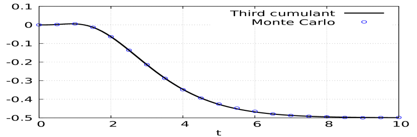
and therefore the third cumulant of X t subscript 𝑋 𝑡 X_{t} 2.2
κ ( 3 ) ( t ) = 2 2 ! λ 3 ( − 27 e − 7 λ t / 6 + 96 e − 3 λ t / 4 − 135 e − 2 λ t / 3 + 4 e − 3 λ t / 2 + 24 e − λ t + 39 e − λ t / 2 − 1 ) , superscript 𝜅 3 𝑡 2 2 superscript 𝜆 3 27 superscript e 7 𝜆 𝑡 6 96 superscript e 3 𝜆 𝑡 4 135 superscript e 2 𝜆 𝑡 3 4 superscript e 3 𝜆 𝑡 2 24 superscript e 𝜆 𝑡 39 superscript e 𝜆 𝑡 2 1 \kappa^{(3)}(t)=2\frac{2!}{\lambda^{3}}\big{(}-27\mathrm{e}^{-7\lambda t/6}+96\mathrm{e}^{-3\lambda t/4}-135\mathrm{e}^{-2\lambda t/3}+4\mathrm{e}^{-3\lambda t/2}+24\mathrm{e}^{-\lambda t}+39\mathrm{e}^{-\lambda t/2}-1\big{)},\quad (5.5)
see Figure 2
Figure 2 : Third cumulant (5.5
From (4.6 5.2 5.5
𝔼 [ ( X t ) 4 ] 𝔼 delimited-[] superscript subscript 𝑋 𝑡 4 \displaystyle\mathbb{E}[(X_{t})^{4}] = \displaystyle= 𝔼 [ ( Y t ) 4 ] − t 4 + 4 t 3 𝔼 [ X t ] − 6 t 2 𝔼 [ ( X t ) 2 ] + 4 t 𝔼 [ X t 3 ] 𝔼 delimited-[] superscript subscript 𝑌 𝑡 4 superscript 𝑡 4 4 superscript 𝑡 3 𝔼 delimited-[] subscript 𝑋 𝑡 6 superscript 𝑡 2 𝔼 delimited-[] superscript subscript 𝑋 𝑡 2 4 𝑡 𝔼 delimited-[] superscript subscript 𝑋 𝑡 3 \displaystyle\mathbb{E}[(Y_{t})^{4}]-t^{4}+4t^{3}\mathbb{E}[X_{t}]-6t^{2}\mathbb{E}[(X_{t})^{2}]+4t\mathbb{E}[X_{t}^{3}]
= \displaystyle= 5 ! λ 4 ( 125 e − 4 λ t / 5 − 256 e − 3 λ t / 4 + 162 e − 2 λ t / 3 − 32 e − λ t / 2 + 1 ) , 5 superscript 𝜆 4 125 superscript e 4 𝜆 𝑡 5 256 superscript e 3 𝜆 𝑡 4 162 superscript e 2 𝜆 𝑡 3 32 superscript e 𝜆 𝑡 2 1 \displaystyle\frac{5!}{\lambda^{4}}\big{(}125\mathrm{e}^{-4\lambda t/5}-256\mathrm{e}^{-3\lambda t/4}+162\mathrm{e}^{-2\lambda t/3}-32\mathrm{e}^{-\lambda t/2}+1\big{)}, (5.6)
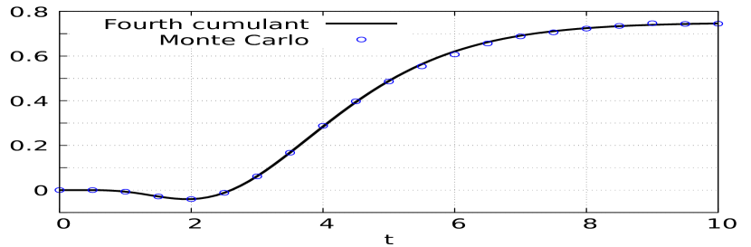
and therefore the fourth cumulant of X t subscript 𝑋 𝑡 X_{t} 2.2
κ ( 4 ) ( t ) superscript 𝜅 4 𝑡 \displaystyle\kappa^{(4)}(t) = \displaystyle= 2 3 ! λ 4 ( − 8 e − 2 λ t + 504 e − 7 λ t / 6 + 1250 e − 4 λ t / 5 − 256 e − 5 λ t / 4 − 2304 e − 3 λ t / 4 \displaystyle 2\frac{3!}{\lambda^{4}}\big{(}-8\mathrm{e}^{-2\lambda t}+504\mathrm{e}^{-7\lambda t/6}+1250\mathrm{e}^{-4\lambda t/5}-256\mathrm{e}^{-5\lambda t/4}-2304\mathrm{e}^{-3\lambda t/4}
+ 72 e − 5 λ t / 3 − 81 e − 4 λ t / 3 + 1206 e − 2 λ t / 3 − 64 e − 3 λ t / 2 − 168 e − λ t − 152 e − λ t / 2 + 1 ) , \displaystyle+72\mathrm{e}^{-5\lambda t/3}-81\mathrm{e}^{-4\lambda t/3}+1206\mathrm{e}^{-2\lambda t/3}-64\mathrm{e}^{-3\lambda t/2}-168\mathrm{e}^{-\lambda t}-152\mathrm{e}^{-\lambda t/2}+1\big{)},
see Figure 3
Figure 3 : Fourth cumulant (5
Proof of Proposition 5.1 ( X t ) t ∈ + subscript subscript 𝑋 𝑡 subscript 𝑡 absent (X_{t})_{t\in_{+}} Boxma et al. ( 2006 ) Daw and Pender ( 2020 ) 𝔼 [ ( X t ) n ] 𝔼 delimited-[] superscript subscript 𝑋 𝑡 𝑛 \mathbb{E}[(X_{t})^{n}]
d d t 𝔼 [ ( X t ) n ] = n 𝔼 [ ( X t ) n − 1 ] − λ n n + 1 𝔼 [ ( X t ) n ] . 𝑑 𝑑 𝑡 𝔼 delimited-[] superscript subscript 𝑋 𝑡 𝑛 𝑛 𝔼 delimited-[] superscript subscript 𝑋 𝑡 𝑛 1 𝜆 𝑛 𝑛 1 𝔼 delimited-[] superscript subscript 𝑋 𝑡 𝑛 \frac{d}{dt}\mathbb{E}[(X_{t})^{n}]=n\mathbb{E}[(X_{t})^{n-1}]-\frac{\lambda n}{n+1}\mathbb{E}[(X_{t})^{n}].
Based on the intuition gained from
(5.2 5.6
𝔼 [ ( X t ) n ] = ( n + 1 ) ! λ n ∑ k = 0 n a k , n e − k λ t / ( k + 1 ) , 𝔼 delimited-[] superscript subscript 𝑋 𝑡 𝑛 𝑛 1 superscript 𝜆 𝑛 superscript subscript 𝑘 0 𝑛 subscript 𝑎 𝑘 𝑛
superscript e 𝑘 𝜆 𝑡 𝑘 1 \mathbb{E}[(X_{t})^{n}]=\frac{(n+1)!}{\lambda^{n}}\sum_{k=0}^{n}a_{k,n}\mathrm{e}^{-k\lambda t/(k+1)},
which, by identification of terms, yields the recurrence relation
a k , n = n ( k + 1 ) n − k a k , n − 1 , 0 ≤ k < n , formulae-sequence subscript 𝑎 𝑘 𝑛
𝑛 𝑘 1 𝑛 𝑘 subscript 𝑎 𝑘 𝑛 1
0 𝑘 𝑛 a_{k,n}=\frac{n(k+1)}{n-k}a_{k,n-1},\qquad 0\leq k<n,
hence
a k , n = ( k + 1 ) n − k ( n k ) a k , k , 0 ≤ k < n . formulae-sequence subscript 𝑎 𝑘 𝑛
superscript 𝑘 1 𝑛 𝑘 binomial 𝑛 𝑘 subscript 𝑎 𝑘 𝑘
0 𝑘 𝑛 a_{k,n}=(k+1)^{n-k}{n\choose k}a_{k,k},\qquad 0\leq k<n.
In addition, the initial condition t = 0 𝑡 0 t=0
∑ k = 0 n a k , n = 0 , superscript subscript 𝑘 0 𝑛 subscript 𝑎 𝑘 𝑛
0 \sum_{k=0}^{n}a_{k,n}=0,
hence
∑ k = 0 n ( k + 1 ) n − k ( n k ) a k , k = 0 , superscript subscript 𝑘 0 𝑛 superscript 𝑘 1 𝑛 𝑘 binomial 𝑛 𝑘 subscript 𝑎 𝑘 𝑘
0 \sum_{k=0}^{n}(k+1)^{n-k}{n\choose k}a_{k,k}=0,
which is solved by taking a k , k = ( − 1 ) k ( k + 1 ) k − 1 subscript 𝑎 𝑘 𝑘
superscript 1 𝑘 superscript 𝑘 1 𝑘 1 a_{k,k}=(-1)^{k}(k+1)^{k-1}
S ( n , n + 1 ) = ∑ k = 0 n ( − 1 ) n − k ( k + 1 ) n ( n + 1 k + 1 ) = ( n + 1 ) ∑ k = 0 n ( k + 1 ) n − 1 ( n k ) ( − 1 ) k = 0 , 𝑆 𝑛 𝑛 1 superscript subscript 𝑘 0 𝑛 superscript 1 𝑛 𝑘 superscript 𝑘 1 𝑛 binomial 𝑛 1 𝑘 1 𝑛 1 superscript subscript 𝑘 0 𝑛 superscript 𝑘 1 𝑛 1 binomial 𝑛 𝑘 superscript 1 𝑘 0 S(n,n+1)=\sum_{k=0}^{n}(-1)^{n-k}(k+1)^{n}{n+1\choose k+1}=(n+1)\sum_{k=0}^{n}(k+1)^{n-1}{n\choose k}(-1)^{k}=0,
which follows from the vanishing of the Stirling numbers
of the second kind S ( n , n + 1 ) 𝑆 𝑛 𝑛 1 S(n,n+1) Abramowitz and Stegun ( 1972 ) □ □ \square
6 Embedded growth-collapse chain
In this section we show that Proposition 2.1
Y ( m ) = Y T m = ∑ k = 1 m g ( T k , k , m ) = ∫ 0 ∞ g ( s , N s , m ) 𝟏 [ 0 , T m ] ( s ) 𝑑 N s , m ≥ 1 . formulae-sequence 𝑌 𝑚 subscript 𝑌 subscript 𝑇 𝑚 superscript subscript 𝑘 1 𝑚 𝑔 subscript 𝑇 𝑘 𝑘 𝑚 superscript subscript 0 𝑔 𝑠 subscript 𝑁 𝑠 𝑚 subscript 1 0 subscript 𝑇 𝑚 𝑠 differential-d subscript 𝑁 𝑠 𝑚 1 Y(m)=Y_{T_{m}}=\sum_{k=1}^{m}g(T_{k},k,m)=\int_{0}^{\infty}g(s,N_{s},m){\bf 1}_{[0,T_{m}]}(s)dN_{s},\qquad m\geq 1. (6.1)
Proposition 6.1
Let ( Y ( m ) ) m ≥ 1 subscript 𝑌 𝑚 𝑚 1 (Y(m))_{m\geq 1} 6.1 n , m ≥ 1 𝑛 𝑚
1 n,m\geq 1
𝔼 [ ( Y ( m ) ) n ] = 𝔼 delimited-[] superscript 𝑌 𝑚 𝑛 absent \displaystyle\mathbb{E}\big{[}(Y(m))^{n}\big{]}=
n ! ∑ k = 1 n λ k ∑ 0 = q 0 < q 1 < ⋯ < q k − 1 < q k = n 𝔼 [ ∫ 0 ∞ ∫ 0 s k ⋯ ∫ 0 s 2 𝟏 { N s k − ≤ m − k } ∏ l = 1 k ( g ( s l , l + N s l , m ) ) q l − q l − 1 ( q l − q l − 1 ) ! d s 1 ⋯ d s k ] . 𝑛 superscript subscript 𝑘 1 𝑛 superscript 𝜆 𝑘 subscript 0 subscript 𝑞 0 subscript 𝑞 1 ⋯ subscript 𝑞 𝑘 1 subscript 𝑞 𝑘 𝑛 𝔼 delimited-[] superscript subscript 0 superscript subscript 0 subscript 𝑠 𝑘 ⋯ superscript subscript 0 subscript 𝑠 2 subscript 1 subscript 𝑁 superscript subscript 𝑠 𝑘 𝑚 𝑘 superscript subscript product 𝑙 1 𝑘 superscript 𝑔 subscript 𝑠 𝑙 𝑙 subscript 𝑁 subscript 𝑠 𝑙 𝑚 subscript 𝑞 𝑙 subscript 𝑞 𝑙 1 subscript 𝑞 𝑙 subscript 𝑞 𝑙 1 𝑑 subscript 𝑠 1 ⋯ 𝑑 subscript 𝑠 𝑘 \displaystyle n!\sum_{k=1}^{n}\lambda^{k}\sum_{0=q_{0}<q_{1}<\cdots<q_{k-1}<q_{k}=n}\mathbb{E}\left[\int_{0}^{\infty}\int_{0}^{s_{k}}\cdots\int_{0}^{s_{2}}{\bf 1}_{\{N_{{s_{k}}^{-}}\leq m-k\}}\prod_{l=1}^{k}\frac{\big{(}g(s_{l},l+N_{s_{l}},m)\big{)}^{q_{l}-q_{l-1}}}{(q_{l}-q_{l-1})!}ds_{1}\cdots ds_{k}\right].
Proof.
By Proposition 2.1 { s ≤ T m } = { N s − < m } 𝑠 subscript 𝑇 𝑚 subscript 𝑁 superscript 𝑠 𝑚 \{s\leq T_{m}\}=\{N_{s^{-}}<m\} s > 0 𝑠 0 s>0 n ≥ 1 𝑛 1 n\geq 1
𝔼 [ ( ∑ k = 1 m g ( T k , k , m ) ) n ] = 𝔼 [ ( ∫ 0 ∞ g ( s , N s , m ) 𝟏 [ 0 , T m ] ( s ) 𝑑 N s ) n ] 𝔼 delimited-[] superscript superscript subscript 𝑘 1 𝑚 𝑔 subscript 𝑇 𝑘 𝑘 𝑚 𝑛 𝔼 delimited-[] superscript superscript subscript 0 𝑔 𝑠 subscript 𝑁 𝑠 𝑚 subscript 1 0 subscript 𝑇 𝑚 𝑠 differential-d subscript 𝑁 𝑠 𝑛 \displaystyle\mathbb{E}\left[\left(\sum_{k=1}^{m}g(T_{k},k,m)\right)^{n}\right]=\mathbb{E}\left[\left(\int_{0}^{\infty}g(s,N_{s},m){\bf 1}_{[0,T_{m}]}(s)dN_{s}\right)^{n}\right]
= ∑ k = 1 n k ! λ k ∑ π 1 ∪ ⋯ ∪ π k = { 1 , … , n } 𝔼 [ ∫ 0 ∞ ∫ 0 s k ⋯ ∫ 0 s 2 ϵ s 1 + ⋯ ϵ s k + ∏ l = 1 k ( g ( s l , N s l , m ) 𝟏 { N s l − < m } ) | π l | d s 1 ⋯ d s k ] absent superscript subscript 𝑘 1 𝑛 𝑘 superscript 𝜆 𝑘 subscript subscript 𝜋 1 ⋯ subscript 𝜋 𝑘 1 … 𝑛 𝔼 delimited-[] superscript subscript 0 superscript subscript 0 subscript 𝑠 𝑘 ⋯ superscript subscript 0 subscript 𝑠 2 subscript superscript italic-ϵ subscript 𝑠 1 ⋯ subscript superscript italic-ϵ subscript 𝑠 𝑘 superscript subscript product 𝑙 1 𝑘 superscript 𝑔 subscript 𝑠 𝑙 subscript 𝑁 subscript 𝑠 𝑙 𝑚 subscript 1 subscript 𝑁 superscript subscript 𝑠 𝑙 𝑚 subscript 𝜋 𝑙 𝑑 subscript 𝑠 1 ⋯ 𝑑 subscript 𝑠 𝑘 \displaystyle=\sum_{k=1}^{n}k!\lambda^{k}\sum_{\pi_{1}\cup\cdots\cup\pi_{k}=\{1,\ldots,n\}}\mathbb{E}\left[\int_{0}^{\infty}\int_{0}^{s_{k}}\cdots\int_{0}^{s_{2}}\epsilon^{+}_{s_{1}}\cdots\epsilon^{+}_{s_{k}}\prod_{l=1}^{k}\big{(}g(s_{l},N_{s_{l}},m){\bf 1}_{\{N_{s_{l}^{-}}<m\}}\big{)}^{|\pi_{l}|}ds_{1}\cdots ds_{k}\right]
= ∑ k = 1 n k ! λ k ∑ π 1 ∪ ⋯ ∪ π k = { 1 , … , n } 𝔼 [ ∫ 0 ∞ ∫ 0 s k ⋯ ∫ 0 s 2 ∏ l = 1 k ( g ( s l , l + N s l , m ) 𝟏 { l − 1 + N s l − < m } ) | π l | d s 1 ⋯ d s k ] absent superscript subscript 𝑘 1 𝑛 𝑘 superscript 𝜆 𝑘 subscript subscript 𝜋 1 ⋯ subscript 𝜋 𝑘 1 … 𝑛 𝔼 delimited-[] superscript subscript 0 superscript subscript 0 subscript 𝑠 𝑘 ⋯ superscript subscript 0 subscript 𝑠 2 superscript subscript product 𝑙 1 𝑘 superscript 𝑔 subscript 𝑠 𝑙 𝑙 subscript 𝑁 subscript 𝑠 𝑙 𝑚 subscript 1 𝑙 1 subscript 𝑁 superscript subscript 𝑠 𝑙 𝑚 subscript 𝜋 𝑙 𝑑 subscript 𝑠 1 ⋯ 𝑑 subscript 𝑠 𝑘 \displaystyle=\sum_{k=1}^{n}k!\lambda^{k}\sum_{\pi_{1}\cup\cdots\cup\pi_{k}=\{1,\ldots,n\}}\mathbb{E}\left[\int_{0}^{\infty}\int_{0}^{s_{k}}\cdots\int_{0}^{s_{2}}\prod_{l=1}^{k}\big{(}g(s_{l},l+N_{s_{l}},m){\bf 1}_{\{l-1+N_{s_{l}^{-}}<m\}}\big{)}^{|\pi_{l}|}ds_{1}\cdots ds_{k}\right]
= ∑ k = 1 n k ! λ k ∑ π 1 ∪ ⋯ ∪ π k = { 1 , … , n } 𝔼 [ ∫ 0 ∞ ∫ 0 s k ⋯ ∫ 0 s 2 𝟏 { N s k − ≤ m − k } ∏ l = 1 k ( g ( s l , l + N s l , m ) ) | π l | d s 1 ⋯ d s k ] . absent superscript subscript 𝑘 1 𝑛 𝑘 superscript 𝜆 𝑘 subscript subscript 𝜋 1 ⋯ subscript 𝜋 𝑘 1 … 𝑛 𝔼 delimited-[] superscript subscript 0 superscript subscript 0 subscript 𝑠 𝑘 ⋯ superscript subscript 0 subscript 𝑠 2 subscript 1 subscript 𝑁 superscript subscript 𝑠 𝑘 𝑚 𝑘 superscript subscript product 𝑙 1 𝑘 superscript 𝑔 subscript 𝑠 𝑙 𝑙 subscript 𝑁 subscript 𝑠 𝑙 𝑚 subscript 𝜋 𝑙 𝑑 subscript 𝑠 1 ⋯ 𝑑 subscript 𝑠 𝑘 \displaystyle=\sum_{k=1}^{n}k!\lambda^{k}\sum_{\pi_{1}\cup\cdots\cup\pi_{k}=\{1,\ldots,n\}}\mathbb{E}\left[\int_{0}^{\infty}\int_{0}^{s_{k}}\cdots\int_{0}^{s_{2}}{\bf 1}_{\{N_{{s_{k}}^{-}}\leq m-k\}}\prod_{l=1}^{k}\big{(}g(s_{l},l+N_{s_{l}},m)\big{)}^{|\pi_{l}|}ds_{1}\cdots ds_{k}\right].
□ □ \square
Next, we specialize Proposition 6.1 g ( s , k , m ) 𝑔 𝑠 𝑘 𝑚 g(s,k,m)
g ( s , k , m ) = f k ( s ) ( 1 − Z k ) ∏ l = k + 1 m Z l , 𝑔 𝑠 𝑘 𝑚 subscript 𝑓 𝑘 𝑠 1 subscript 𝑍 𝑘 superscript subscript product 𝑙 𝑘 1 𝑚 subscript 𝑍 𝑙 g(s,k,m)=f_{k}(s)(1-Z_{k})\prod_{l=k+1}^{m}Z_{l}, (6.2)
where ( Z k ) k ≥ 1 subscript subscript 𝑍 𝑘 𝑘 1 (Z_{k})_{k\geq 1} ( N t ) t ∈ + subscript subscript 𝑁 𝑡 subscript 𝑡 absent (N_{t})_{t\in_{+}} m n = 𝔼 [ Z n ] subscript 𝑚 𝑛 𝔼 delimited-[] superscript 𝑍 𝑛 m_{n}=\mathbb{E}[Z^{n}] n ≥ 0 𝑛 0 n\geq 0
Corollary 6.2
Let ( Y ( m ) ) m ≥ 1 subscript 𝑌 𝑚 𝑚 1 (Y(m))_{m\geq 1} 6.2 n , m ≥ 1 𝑛 𝑚
1 n,m\geq 1
𝔼 [ ( Y ( m ) ) n ] = n ! ∑ k = 1 n ∑ i = 0 m − k λ k + i i ! m n m − i − k ∑ 0 = q 0 < q 1 < ⋯ < q k − 1 < q k = n 𝔼 delimited-[] superscript 𝑌 𝑚 𝑛 𝑛 superscript subscript 𝑘 1 𝑛 superscript subscript 𝑖 0 𝑚 𝑘 superscript 𝜆 𝑘 𝑖 𝑖 superscript subscript 𝑚 𝑛 𝑚 𝑖 𝑘 subscript 0 subscript 𝑞 0 subscript 𝑞 1 ⋯ subscript 𝑞 𝑘 1 subscript 𝑞 𝑘 𝑛 \displaystyle\mathbb{E}\big{[}(Y(m))^{n}\big{]}=n!\sum_{k=1}^{n}\sum_{i=0}^{m-k}\frac{\lambda^{k+i}}{i!}m_{n}^{m-i-k}\sum_{0=q_{0}<q_{1}<\cdots<q_{k-1}<q_{k}=n}
∏ l = 1 k C q l − 1 , q l − q l − 1 ( q l − q l − 1 ) ! ∫ 0 ∞ e − λ s k ∫ 0 s k ⋯ ∫ 0 s 2 ( s 1 + ∑ l = 1 k − 1 m p 1 + ⋯ + p l ( s l + 1 − s l ) ) i ∏ l = 1 k f l , m q l − q l − 1 ( s l ) d s 1 ⋯ d s k . superscript subscript product 𝑙 1 𝑘 subscript 𝐶 subscript 𝑞 𝑙 1 subscript 𝑞 𝑙 subscript 𝑞 𝑙 1
subscript 𝑞 𝑙 subscript 𝑞 𝑙 1 superscript subscript 0 superscript e 𝜆 subscript 𝑠 𝑘 superscript subscript 0 subscript 𝑠 𝑘 ⋯ superscript subscript 0 subscript 𝑠 2 superscript subscript 𝑠 1 superscript subscript 𝑙 1 𝑘 1 subscript 𝑚 subscript 𝑝 1 ⋯ subscript 𝑝 𝑙 subscript 𝑠 𝑙 1 subscript 𝑠 𝑙 𝑖 superscript subscript product 𝑙 1 𝑘 superscript subscript 𝑓 𝑙 𝑚
subscript 𝑞 𝑙 subscript 𝑞 𝑙 1 subscript 𝑠 𝑙 𝑑 subscript 𝑠 1 ⋯ 𝑑 subscript 𝑠 𝑘 \displaystyle\prod_{l=1}^{k}\frac{C_{q_{l-1},q_{l}-q_{l-1}}}{(q_{l}-q_{l-1})!}\int_{0}^{\infty}\mathrm{e}^{-\lambda s_{k}}\int_{0}^{s_{k}}\cdots\int_{0}^{s_{2}}\left(s_{1}+\sum_{l=1}^{k-1}m_{p_{1}+\cdots+p_{l}}(s_{l+1}-s_{l})\right)^{i}\prod_{l=1}^{k}f_{l,m}^{q_{l}-q_{l-1}}(s_{l})ds_{1}\cdots ds_{k}.
Proof.
Using the fact that the jumps of ( N s ) s ∈ [ 0 , s k ] subscript subscript 𝑁 𝑠 𝑠 0 subscript 𝑠 𝑘 (N_{s})_{s\in[0,s_{k}]} [ 0 , s k ] 0 subscript 𝑠 𝑘 [0,s_{k}] N s k = i subscript 𝑁 subscript 𝑠 𝑘 𝑖 N_{s_{k}}=i 6.1
𝔼 [ ( ∑ k = 1 m g ( T k , k , m ) ) n ] = ∑ k = 1 n k ! λ k ∑ π 1 ∪ ⋯ ∪ π k = { 1 , … , n } 𝔼 delimited-[] superscript superscript subscript 𝑘 1 𝑚 𝑔 subscript 𝑇 𝑘 𝑘 𝑚 𝑛 superscript subscript 𝑘 1 𝑛 𝑘 superscript 𝜆 𝑘 subscript subscript 𝜋 1 ⋯ subscript 𝜋 𝑘 1 … 𝑛 \displaystyle\mathbb{E}\left[\left(\sum_{k=1}^{m}g(T_{k},k,m)\right)^{n}\right]=\sum_{k=1}^{n}k!\lambda^{k}\sum_{\pi_{1}\cup\cdots\cup\pi_{k}=\{1,\ldots,n\}}
𝔼 [ ∫ 0 ∞ ∫ 0 s k ⋯ ∫ 0 s 2 𝟏 { N s k − ≤ m − k } ∏ l = 1 k ( f l , m ( s l ) ( 1 − Z l + N s l ) ∏ j = l + 1 + N s l m Z j ) | π l | d s 1 ⋯ d s k ] 𝔼 delimited-[] superscript subscript 0 superscript subscript 0 subscript 𝑠 𝑘 ⋯ superscript subscript 0 subscript 𝑠 2 subscript 1 subscript 𝑁 superscript subscript 𝑠 𝑘 𝑚 𝑘 superscript subscript product 𝑙 1 𝑘 superscript subscript 𝑓 𝑙 𝑚
subscript 𝑠 𝑙 1 subscript 𝑍 𝑙 subscript 𝑁 subscript 𝑠 𝑙 superscript subscript product 𝑗 𝑙 1 subscript 𝑁 subscript 𝑠 𝑙 𝑚 subscript 𝑍 𝑗 subscript 𝜋 𝑙 𝑑 subscript 𝑠 1 ⋯ 𝑑 subscript 𝑠 𝑘 \displaystyle\quad\mathbb{E}\left[\int_{0}^{\infty}\int_{0}^{s_{k}}\cdots\int_{0}^{s_{2}}{\bf 1}_{\{N_{{s_{k}}^{-}}\leq m-k\}}\prod_{l=1}^{k}\left(f_{l,m}(s_{l})(1-Z_{l+N_{s_{l}}})\prod_{j=l+1+N_{s_{l}}}^{m}Z_{j}\right)^{|\pi_{l}|}ds_{1}\cdots ds_{k}\right]
= ∑ k = 1 n k ! λ k ∑ π 1 ∪ ⋯ ∪ π k = { 1 , … , n } absent superscript subscript 𝑘 1 𝑛 𝑘 superscript 𝜆 𝑘 subscript subscript 𝜋 1 ⋯ subscript 𝜋 𝑘 1 … 𝑛 \displaystyle=\sum_{k=1}^{n}k!\lambda^{k}\sum_{\pi_{1}\cup\cdots\cup\pi_{k}=\{1,\ldots,n\}}
𝔼 [ ∫ 0 ∞ ∫ 0 s k ⋯ ∫ 0 s 2 𝟏 { N s k − ≤ m − k } ∏ l = 1 k ( f l , m p l ( s l ) C p 1 + ⋯ + p l − 1 , p l ( m p 1 + ⋯ + p l ) N s l + 1 − N s l ) d s 1 ⋯ d s k ] 𝔼 delimited-[] superscript subscript 0 superscript subscript 0 subscript 𝑠 𝑘 ⋯ superscript subscript 0 subscript 𝑠 2 subscript 1 subscript 𝑁 superscript subscript 𝑠 𝑘 𝑚 𝑘 superscript subscript product 𝑙 1 𝑘 superscript subscript 𝑓 𝑙 𝑚
subscript 𝑝 𝑙 subscript 𝑠 𝑙 subscript 𝐶 subscript 𝑝 1 ⋯ subscript 𝑝 𝑙 1 subscript 𝑝 𝑙
superscript subscript 𝑚 subscript 𝑝 1 ⋯ subscript 𝑝 𝑙 subscript 𝑁 subscript 𝑠 𝑙 1 subscript 𝑁 subscript 𝑠 𝑙 𝑑 subscript 𝑠 1 ⋯ 𝑑 subscript 𝑠 𝑘 \displaystyle\quad\mathbb{E}\left[\int_{0}^{\infty}\int_{0}^{s_{k}}\cdots\int_{0}^{s_{2}}{\bf 1}_{\{N_{{s_{k}}^{-}}\leq m-k\}}\prod_{l=1}^{k}\left(f_{l,m}^{p_{l}}(s_{l})C_{p_{1}+\cdots+p_{l-1},p_{l}}(m_{p_{1}+\cdots+p_{l}})^{N_{s_{l+1}}-N_{s_{l}}}\right)ds_{1}\cdots ds_{k}\right]
= n ! ∑ k = 1 n λ k p 1 ! ⋯ p k ! ∑ i = 0 m − k ℙ ( N s k − = i ) ∑ p 1 + ⋯ + p k = n p 1 , … , p k ≥ 1 absent 𝑛 superscript subscript 𝑘 1 𝑛 superscript 𝜆 𝑘 subscript 𝑝 1 ⋯ subscript 𝑝 𝑘 superscript subscript 𝑖 0 𝑚 𝑘 ℙ subscript 𝑁 superscript subscript 𝑠 𝑘 𝑖 subscript FRACOP subscript 𝑝 1 ⋯ subscript 𝑝 𝑘 𝑛 subscript 𝑝 1 … subscript 𝑝 𝑘
1 \displaystyle=n!\sum_{k=1}^{n}\frac{\lambda^{k}}{p_{1}!\cdots p_{k}!}\sum_{i=0}^{m-k}{\mathord{\mathbb{P}}}(N_{{s_{k}}^{-}}=i)\sum_{p_{1}+\cdots+p_{k}=n\atop p_{1},\ldots,p_{k}\geq 1}
∫ 0 ∞ ∫ 0 s k ⋯ ∫ 0 s 2 ∏ l = 1 k ( f l , m p l ( s l ) C p 1 + ⋯ + p l − 1 , p l ) ( s 1 + ∑ l = 1 k − 1 m p 1 + ⋯ + p l ( s l + 1 − s l ) s k ) i m n m − i − k d s 1 ⋯ d s k superscript subscript 0 superscript subscript 0 subscript 𝑠 𝑘 ⋯ superscript subscript 0 subscript 𝑠 2 superscript subscript product 𝑙 1 𝑘 superscript subscript 𝑓 𝑙 𝑚
subscript 𝑝 𝑙 subscript 𝑠 𝑙 subscript 𝐶 subscript 𝑝 1 ⋯ subscript 𝑝 𝑙 1 subscript 𝑝 𝑙
superscript subscript 𝑠 1 superscript subscript 𝑙 1 𝑘 1 subscript 𝑚 subscript 𝑝 1 ⋯ subscript 𝑝 𝑙 subscript 𝑠 𝑙 1 subscript 𝑠 𝑙 subscript 𝑠 𝑘 𝑖 superscript subscript 𝑚 𝑛 𝑚 𝑖 𝑘 𝑑 subscript 𝑠 1 ⋯ 𝑑 subscript 𝑠 𝑘 \displaystyle\quad\int_{0}^{\infty}\int_{0}^{s_{k}}\cdots\int_{0}^{s_{2}}\prod_{l=1}^{k}\big{(}f_{l,m}^{p_{l}}(s_{l})C_{p_{1}+\cdots+p_{l-1},p_{l}}\big{)}\left(\frac{s_{1}+\sum_{l=1}^{k-1}m_{p_{1}+\cdots+p_{l}}(s_{l+1}-s_{l})}{s_{k}}\right)^{i}m_{n}^{m-i-k}ds_{1}\cdots ds_{k}
= n ! ∑ k = 1 n λ k + i ∑ p 1 + ⋯ + p k = n p 1 , … , p k ≥ 1 ∑ i = 0 m − k m n m − i − k i ! ∏ l = 1 k C p 1 + ⋯ + p l − 1 , p l p l ! absent 𝑛 superscript subscript 𝑘 1 𝑛 superscript 𝜆 𝑘 𝑖 subscript FRACOP subscript 𝑝 1 ⋯ subscript 𝑝 𝑘 𝑛 subscript 𝑝 1 … subscript 𝑝 𝑘
1 superscript subscript 𝑖 0 𝑚 𝑘 superscript subscript 𝑚 𝑛 𝑚 𝑖 𝑘 𝑖 superscript subscript product 𝑙 1 𝑘 subscript 𝐶 subscript 𝑝 1 ⋯ subscript 𝑝 𝑙 1 subscript 𝑝 𝑙
subscript 𝑝 𝑙 \displaystyle=n!\sum_{k=1}^{n}\lambda^{k+i}\sum_{p_{1}+\cdots+p_{k}=n\atop p_{1},\ldots,p_{k}\geq 1}\sum_{i=0}^{m-k}\frac{m_{n}^{m-i-k}}{i!}\prod_{l=1}^{k}\frac{C_{p_{1}+\cdots+p_{l-1},p_{l}}}{p_{l}!}
∫ 0 ∞ e − λ s k ∫ 0 s k ⋯ ∫ 0 s 2 ∏ l = 1 k f l , m p l ( s l ) ( s 1 + ∑ l = 1 k − 1 m p 1 + ⋯ + p l ( s l + 1 − s l ) ) i d s 1 ⋯ d s k . superscript subscript 0 superscript e 𝜆 subscript 𝑠 𝑘 superscript subscript 0 subscript 𝑠 𝑘 ⋯ superscript subscript 0 subscript 𝑠 2 superscript subscript product 𝑙 1 𝑘 superscript subscript 𝑓 𝑙 𝑚
subscript 𝑝 𝑙 subscript 𝑠 𝑙 superscript subscript 𝑠 1 superscript subscript 𝑙 1 𝑘 1 subscript 𝑚 subscript 𝑝 1 ⋯ subscript 𝑝 𝑙 subscript 𝑠 𝑙 1 subscript 𝑠 𝑙 𝑖 𝑑 subscript 𝑠 1 ⋯ 𝑑 subscript 𝑠 𝑘 \displaystyle\quad\int_{0}^{\infty}\mathrm{e}^{-\lambda s_{k}}\int_{0}^{s_{k}}\cdots\int_{0}^{s_{2}}\prod_{l=1}^{k}f_{l,m}^{p_{l}}(s_{l})\left(s_{1}+\sum_{l=1}^{k-1}m_{p_{1}+\cdots+p_{l}}(s_{l+1}-s_{l})\right)^{i}ds_{1}\cdots ds_{k}.
□ □ \square
Uniform cut-offs
The next result specializes Corollary 6.2
Corollary 6.3
Let ( Y ( m ) ) m ≥ 1 subscript 𝑌 𝑚 𝑚 1 (Y(m))_{m\geq 1} 6.2 ( Z k ) k ≥ 1 subscript subscript 𝑍 𝑘 𝑘 1 (Z_{k})_{k\geq 1} n , m ≥ 1 𝑛 𝑚
1 n,m\geq 1
𝔼 [ ( Y ( m ) ) n ] 𝔼 delimited-[] superscript 𝑌 𝑚 𝑛 \displaystyle\mathbb{E}\big{[}(Y(m))^{n}\big{]} = \displaystyle= ∑ k = 1 n ∑ i = 0 m − k λ k + i i ! ( n + 1 ) m − i − k ∑ 0 = q 0 < q 1 < ⋯ < q k − 1 < q k = n ∏ l = 1 k 1 1 + q l superscript subscript 𝑘 1 𝑛 superscript subscript 𝑖 0 𝑚 𝑘 superscript 𝜆 𝑘 𝑖 𝑖 superscript 𝑛 1 𝑚 𝑖 𝑘 subscript 0 subscript 𝑞 0 subscript 𝑞 1 ⋯ subscript 𝑞 𝑘 1 subscript 𝑞 𝑘 𝑛 superscript subscript product 𝑙 1 𝑘 1 1 subscript 𝑞 𝑙 \displaystyle\sum_{k=1}^{n}\sum_{i=0}^{m-k}\frac{\lambda^{k+i}}{i!(n+1)^{m-i-k}}\sum_{0=q_{0}<q_{1}<\cdots<q_{k-1}<q_{k}=n}\prod_{l=1}^{k}\frac{1}{1+q_{l}}
∫ 0 ∞ e − λ s k ∫ 0 s k ⋯ ∫ 0 s 2 ( s 1 + ∑ l = 1 k − 1 s l + 1 − s l 1 + q l ) i ∏ l = 1 k f l , m q l − q l − 1 ( s l ) d s 1 ⋯ d s k . superscript subscript 0 superscript e 𝜆 subscript 𝑠 𝑘 superscript subscript 0 subscript 𝑠 𝑘 ⋯ superscript subscript 0 subscript 𝑠 2 superscript subscript 𝑠 1 superscript subscript 𝑙 1 𝑘 1 subscript 𝑠 𝑙 1 subscript 𝑠 𝑙 1 subscript 𝑞 𝑙 𝑖 superscript subscript product 𝑙 1 𝑘 superscript subscript 𝑓 𝑙 𝑚
subscript 𝑞 𝑙 subscript 𝑞 𝑙 1 subscript 𝑠 𝑙 𝑑 subscript 𝑠 1 ⋯ 𝑑 subscript 𝑠 𝑘 \displaystyle\quad\int_{0}^{\infty}\mathrm{e}^{-\lambda s_{k}}\int_{0}^{s_{k}}\cdots\int_{0}^{s_{2}}\left(s_{1}+\sum_{l=1}^{k-1}\frac{s_{l+1}-s_{l}}{1+q_{l}}\right)^{i}\prod_{l=1}^{k}f_{l,m}^{q_{l}-q_{l-1}}(s_{l})ds_{1}\cdots ds_{k}.
Proof.
By Corollary 6.2
𝔼 [ ( ∑ k = 1 m g ( T k , k , m ) ) n ] = n ! ∑ k = 1 n λ k + i ∑ p 1 + ⋯ + p k = n p 1 , … , p k ≥ 1 ∑ i = 0 m − k m n m − i − k i ! ∏ l = 1 k C p 1 + ⋯ + p l − 1 , p l p l ! 𝔼 delimited-[] superscript superscript subscript 𝑘 1 𝑚 𝑔 subscript 𝑇 𝑘 𝑘 𝑚 𝑛 𝑛 superscript subscript 𝑘 1 𝑛 superscript 𝜆 𝑘 𝑖 subscript FRACOP subscript 𝑝 1 ⋯ subscript 𝑝 𝑘 𝑛 subscript 𝑝 1 … subscript 𝑝 𝑘
1 superscript subscript 𝑖 0 𝑚 𝑘 superscript subscript 𝑚 𝑛 𝑚 𝑖 𝑘 𝑖 superscript subscript product 𝑙 1 𝑘 subscript 𝐶 subscript 𝑝 1 ⋯ subscript 𝑝 𝑙 1 subscript 𝑝 𝑙
subscript 𝑝 𝑙 \displaystyle\mathbb{E}\left[\left(\sum_{k=1}^{m}g(T_{k},k,m)\right)^{n}\right]=n!\sum_{k=1}^{n}\lambda^{k+i}\sum_{p_{1}+\cdots+p_{k}=n\atop p_{1},\ldots,p_{k}\geq 1}\sum_{i=0}^{m-k}\frac{m_{n}^{m-i-k}}{i!}\prod_{l=1}^{k}\frac{C_{p_{1}+\cdots+p_{l-1},p_{l}}}{p_{l}!}
∫ 0 ∞ e − λ s k ∫ 0 s k ⋯ ∫ 0 s 2 ∏ l = 1 k f l , m p l ( s l ) ( s 1 + ∑ l = 1 k − 1 m p 1 + ⋯ + p l ( s l + 1 − s l ) ) i d s 1 ⋯ d s k superscript subscript 0 superscript e 𝜆 subscript 𝑠 𝑘 superscript subscript 0 subscript 𝑠 𝑘 ⋯ superscript subscript 0 subscript 𝑠 2 superscript subscript product 𝑙 1 𝑘 superscript subscript 𝑓 𝑙 𝑚
subscript 𝑝 𝑙 subscript 𝑠 𝑙 superscript subscript 𝑠 1 superscript subscript 𝑙 1 𝑘 1 subscript 𝑚 subscript 𝑝 1 ⋯ subscript 𝑝 𝑙 subscript 𝑠 𝑙 1 subscript 𝑠 𝑙 𝑖 𝑑 subscript 𝑠 1 ⋯ 𝑑 subscript 𝑠 𝑘 \displaystyle\int_{0}^{\infty}\mathrm{e}^{-\lambda s_{k}}\int_{0}^{s_{k}}\cdots\int_{0}^{s_{2}}\prod_{l=1}^{k}f_{l,m}^{p_{l}}(s_{l})\left(s_{1}+\sum_{l=1}^{k-1}m_{p_{1}+\cdots+p_{l}}(s_{l+1}-s_{l})\right)^{i}ds_{1}\cdots ds_{k}
= \displaystyle= n ! ∑ k = 1 n λ k + i ∑ p 1 + ⋯ + p k = n p 1 , … , p k ≥ 1 ∑ i = 0 m − k m n m − i − k i ! ∏ l = 1 k ( p 1 + ⋯ + p l − 1 ) ! ( p 1 + ⋯ + p l + 1 ) ! 𝑛 superscript subscript 𝑘 1 𝑛 superscript 𝜆 𝑘 𝑖 subscript FRACOP subscript 𝑝 1 ⋯ subscript 𝑝 𝑘 𝑛 subscript 𝑝 1 … subscript 𝑝 𝑘
1 superscript subscript 𝑖 0 𝑚 𝑘 superscript subscript 𝑚 𝑛 𝑚 𝑖 𝑘 𝑖 superscript subscript product 𝑙 1 𝑘 subscript 𝑝 1 ⋯ subscript 𝑝 𝑙 1 subscript 𝑝 1 ⋯ subscript 𝑝 𝑙 1 \displaystyle n!\sum_{k=1}^{n}\lambda^{k+i}\sum_{p_{1}+\cdots+p_{k}=n\atop p_{1},\ldots,p_{k}\geq 1}\sum_{i=0}^{m-k}\frac{m_{n}^{m-i-k}}{i!}\prod_{l=1}^{k}\frac{(p_{1}+\cdots+p_{l-1})!}{(p_{1}+\cdots+p_{l}+1)!}
∫ 0 ∞ e − λ s k ∫ 0 s k ⋯ ∫ 0 s 2 ∏ l = 1 k f l , m p l ( s l ) ( s 1 + ∑ l = 1 k − 1 m p 1 + ⋯ + p l ( s l + 1 − s l ) ) i d s 1 ⋯ d s k . superscript subscript 0 superscript e 𝜆 subscript 𝑠 𝑘 superscript subscript 0 subscript 𝑠 𝑘 ⋯ superscript subscript 0 subscript 𝑠 2 superscript subscript product 𝑙 1 𝑘 superscript subscript 𝑓 𝑙 𝑚
subscript 𝑝 𝑙 subscript 𝑠 𝑙 superscript subscript 𝑠 1 superscript subscript 𝑙 1 𝑘 1 subscript 𝑚 subscript 𝑝 1 ⋯ subscript 𝑝 𝑙 subscript 𝑠 𝑙 1 subscript 𝑠 𝑙 𝑖 𝑑 subscript 𝑠 1 ⋯ 𝑑 subscript 𝑠 𝑘 \displaystyle\int_{0}^{\infty}\mathrm{e}^{-\lambda s_{k}}\int_{0}^{s_{k}}\cdots\int_{0}^{s_{2}}\prod_{l=1}^{k}f_{l,m}^{p_{l}}(s_{l})\left(s_{1}+\sum_{l=1}^{k-1}m_{p_{1}+\cdots+p_{l}}(s_{l+1}-s_{l})\right)^{i}ds_{1}\cdots ds_{k}.
□ □ \square
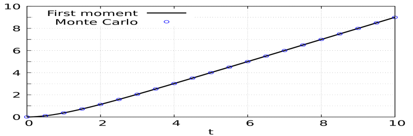
The first moments of Y ( m ) 𝑌 𝑚 Y(m) f l , m ( s ) = s subscript 𝑓 𝑙 𝑚
𝑠 𝑠 f_{l,m}(s)=s
Y ( m ) = Y T m = ∑ k = 1 m T k ( 1 − U k ) ∏ l = k + 1 m U l , m ≥ 1 , formulae-sequence 𝑌 𝑚 subscript 𝑌 subscript 𝑇 𝑚 superscript subscript 𝑘 1 𝑚 subscript 𝑇 𝑘 1 subscript 𝑈 𝑘 superscript subscript product 𝑙 𝑘 1 𝑚 subscript 𝑈 𝑙 𝑚 1 Y(m)=Y_{T_{m}}=\sum_{k=1}^{m}T_{k}(1-U_{k})\prod_{l=k+1}^{m}U_{l},\qquad m\geq 1,
where ( U k ) k ≥ 1 subscript subscript 𝑈 𝑘 𝑘 1 (U_{k})_{k\geq 1} [ 0 , 1 ] 0 1 [0,1]
First moment
For n = 1 𝑛 1 n=1 6.3
𝔼 [ Y ( m ) ] = 1 λ ∑ i = 0 m − 1 1 i ! 2 m − i − 1 ∫ 0 ∞ e − s 1 s 1 i s 1 2 𝑑 s 1 = 2 − m + m − 1 λ , 𝔼 delimited-[] 𝑌 𝑚 1 𝜆 superscript subscript 𝑖 0 𝑚 1 1 𝑖 superscript 2 𝑚 𝑖 1 superscript subscript 0 superscript e subscript 𝑠 1 superscript subscript 𝑠 1 𝑖 subscript 𝑠 1 2 differential-d subscript 𝑠 1 superscript 2 𝑚 𝑚 1 𝜆 \mathbb{E}\big{[}Y(m)\big{]}=\frac{1}{\lambda}\sum_{i=0}^{m-1}\frac{1}{i!2^{m-i-1}}\int_{0}^{\infty}\mathrm{e}^{-s_{1}}s_{1}^{i}\frac{s_{1}}{2}ds_{1}=\frac{2^{-m}+m-1}{\lambda},
which is consistent with Theorem 7 in Boxma et al. ( 2006 )
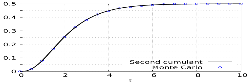
Second moment
For n = 2 𝑛 2 n=2
𝔼 [ ( Y ( m ) ) 2 ] 𝔼 delimited-[] superscript 𝑌 𝑚 2 \displaystyle\mathbb{E}\big{[}(Y(m))^{2}\big{]}
= 1 λ 2 ∑ i = 0 m − 1 1 i ! 3 m − 1 − i ∫ 0 ∞ e − s 1 s 1 i s 1 2 3 𝑑 s 1 + 1 2 λ 2 ∑ i = 0 m − 2 1 i ! 3 m − 2 − i ∫ 0 ∞ e − s 2 ∫ 0 s 2 ( s 1 + s 2 2 ) i s 1 s 2 3 𝑑 s 1 𝑑 s 2 absent 1 superscript 𝜆 2 superscript subscript 𝑖 0 𝑚 1 1 𝑖 superscript 3 𝑚 1 𝑖 superscript subscript 0 superscript e subscript 𝑠 1 superscript subscript 𝑠 1 𝑖 superscript subscript 𝑠 1 2 3 differential-d subscript 𝑠 1 1 2 superscript 𝜆 2 superscript subscript 𝑖 0 𝑚 2 1 𝑖 superscript 3 𝑚 2 𝑖 superscript subscript 0 superscript e subscript 𝑠 2 superscript subscript 0 subscript 𝑠 2 superscript subscript 𝑠 1 subscript 𝑠 2 2 𝑖 subscript 𝑠 1 subscript 𝑠 2 3 differential-d subscript 𝑠 1 differential-d subscript 𝑠 2 \displaystyle=\frac{1}{\lambda^{2}}\sum_{i=0}^{m-1}\frac{1}{i!3^{m-1-i}}\int_{0}^{\infty}\mathrm{e}^{-s_{1}}s_{1}^{i}\frac{s_{1}^{2}}{3}ds_{1}+\frac{1}{2\lambda^{2}}\sum_{i=0}^{m-2}\frac{1}{i!3^{m-2-i}}\int_{0}^{\infty}\mathrm{e}^{-s_{2}}\int_{0}^{s_{2}}\left(\frac{s_{1}+s_{2}}{2}\right)^{i}s_{1}\frac{s_{2}}{3}ds_{1}ds_{2}
= 1 λ 2 ( 2 3 m + m − 1 2 m − 1 − m + m 2 ) . absent 1 superscript 𝜆 2 2 superscript 3 𝑚 𝑚 1 superscript 2 𝑚 1 𝑚 superscript 𝑚 2 \displaystyle=\frac{1}{\lambda^{2}}\left(\frac{2}{3^{m}}+\frac{m-1}{2^{m-1}}-m+m^{2}\right).
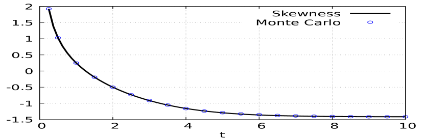
Third moment
For n = 3 𝑛 3 n=3
𝔼 [ Y ( m ) 3 ] 𝔼 delimited-[] 𝑌 superscript 𝑚 3 \displaystyle\mathbb{E}\big{[}Y(m)^{3}\big{]} = \displaystyle= 1 λ 3 ∑ i = 0 m − 1 1 i ! 4 m − 1 − i ∫ 0 ∞ e − s 1 s 1 i + 3 4 𝑑 s 1 1 superscript 𝜆 3 superscript subscript 𝑖 0 𝑚 1 1 𝑖 superscript 4 𝑚 1 𝑖 superscript subscript 0 superscript e subscript 𝑠 1 superscript subscript 𝑠 1 𝑖 3 4 differential-d subscript 𝑠 1 \displaystyle\frac{1}{\lambda^{3}}\sum_{i=0}^{m-1}\frac{1}{i!4^{m-1-i}}\int_{0}^{\infty}\mathrm{e}^{-s_{1}}\frac{s_{1}^{i+3}}{4}ds_{1} (6.5)
+ 1 λ 3 ∑ i = 0 m − 2 1 i ! 4 m − 2 − i ∫ 0 ∞ e − s 2 ∫ 0 s 2 ( ( s 1 + s 2 2 ) i s 1 2 s 2 2 4 + ( 2 s 1 + s 2 3 ) i s 1 2 3 s 2 4 ) 𝑑 s 1 𝑑 s 2 1 superscript 𝜆 3 superscript subscript 𝑖 0 𝑚 2 1 𝑖 superscript 4 𝑚 2 𝑖 superscript subscript 0 superscript e subscript 𝑠 2 superscript subscript 0 subscript 𝑠 2 superscript subscript 𝑠 1 subscript 𝑠 2 2 𝑖 subscript 𝑠 1 2 superscript subscript 𝑠 2 2 4 superscript 2 subscript 𝑠 1 subscript 𝑠 2 3 𝑖 superscript subscript 𝑠 1 2 3 subscript 𝑠 2 4 differential-d subscript 𝑠 1 differential-d subscript 𝑠 2 \displaystyle+\frac{1}{\lambda^{3}}\sum_{i=0}^{m-2}\frac{1}{i!4^{m-2-i}}\int_{0}^{\infty}\mathrm{e}^{-s_{2}}\int_{0}^{s_{2}}\left(\left(\frac{s_{1}+s_{2}}{2}\right)^{i}\frac{s_{1}}{2}\frac{s_{2}^{2}}{4}+\left(\frac{2s_{1}+s_{2}}{3}\right)^{i}\frac{s_{1}^{2}}{3}\frac{s_{2}}{4}\right)ds_{1}ds_{2}
+ 1 λ 3 ∑ i = 0 m − 3 1 i ! 4 m − 3 − i ∫ 0 ∞ e − s 3 ∫ 0 s 3 ∫ 0 s 2 ( 3 s 1 + s 2 + 2 s 3 6 ) i s 1 2 s 2 3 s 3 4 𝑑 s 1 𝑑 s 2 𝑑 s 3 . 1 superscript 𝜆 3 superscript subscript 𝑖 0 𝑚 3 1 𝑖 superscript 4 𝑚 3 𝑖 superscript subscript 0 superscript e subscript 𝑠 3 superscript subscript 0 subscript 𝑠 3 superscript subscript 0 subscript 𝑠 2 superscript 3 subscript 𝑠 1 subscript 𝑠 2 2 subscript 𝑠 3 6 𝑖 subscript 𝑠 1 2 subscript 𝑠 2 3 subscript 𝑠 3 4 differential-d subscript 𝑠 1 differential-d subscript 𝑠 2 differential-d subscript 𝑠 3 \displaystyle+\frac{1}{\lambda^{3}}\sum_{i=0}^{m-3}\frac{1}{i!4^{m-3-i}}\int_{0}^{\infty}\mathrm{e}^{-s_{3}}\int_{0}^{s_{3}}\int_{0}^{s_{2}}\left(\frac{3s_{1}+s_{2}+2s_{3}}{6}\right)^{i}\frac{s_{1}}{2}\frac{s_{2}}{3}\frac{s_{3}}{4}ds_{1}ds_{2}ds_{3}.
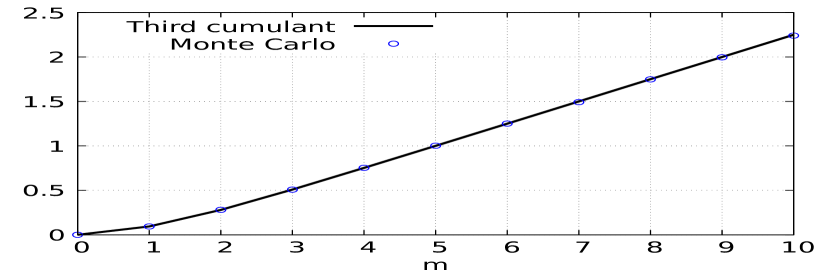
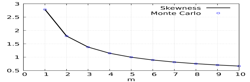
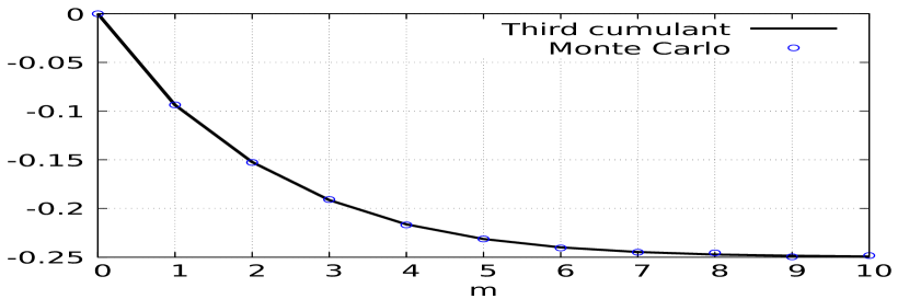
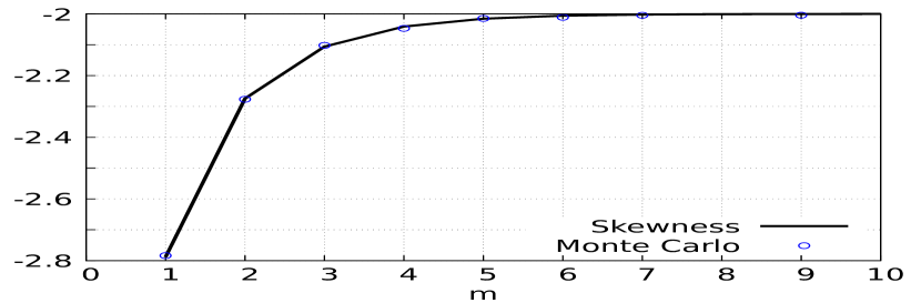
Although the last partial summation (6.5 4
Figure 4 : Third cumulant and skewness of Y ( m ) 𝑌 𝑚 Y(m)
Fourth moment
For n = 4 𝑛 4 n=4
𝔼 [ Y ( m ) 4 ] = 1 λ 4 ∑ i = 0 m − 1 1 i ! 5 m − 1 − i ∫ 0 ∞ e − s 1 s 1 i + 4 5 𝑑 s 1 𝔼 delimited-[] 𝑌 superscript 𝑚 4 1 superscript 𝜆 4 superscript subscript 𝑖 0 𝑚 1 1 𝑖 superscript 5 𝑚 1 𝑖 superscript subscript 0 superscript e subscript 𝑠 1 superscript subscript 𝑠 1 𝑖 4 5 differential-d subscript 𝑠 1 \displaystyle\mathbb{E}\big{[}Y(m)^{4}\big{]}=\frac{1}{\lambda^{4}}\sum_{i=0}^{m-1}\frac{1}{i!5^{m-1-i}}\int_{0}^{\infty}\mathrm{e}^{-s_{1}}\frac{s_{1}^{i+4}}{5}ds_{1}
+ 1 λ 4 ∑ i = 0 m − 2 1 i ! 5 m − 2 − i ∫ 0 ∞ e − s 2 ∫ 0 s 2 ( ( s 1 + s 2 2 ) i s 1 2 s 2 3 5 + ( 3 s 1 + s 2 4 ) i s 1 3 4 s 2 5 + ( 2 s 1 + s 2 3 ) i s 1 2 3 s 2 2 5 ) 𝑑 s 1 𝑑 s 2 1 superscript 𝜆 4 superscript subscript 𝑖 0 𝑚 2 1 𝑖 superscript 5 𝑚 2 𝑖 superscript subscript 0 superscript e subscript 𝑠 2 superscript subscript 0 subscript 𝑠 2 superscript subscript 𝑠 1 subscript 𝑠 2 2 𝑖 subscript 𝑠 1 2 superscript subscript 𝑠 2 3 5 superscript 3 subscript 𝑠 1 subscript 𝑠 2 4 𝑖 superscript subscript 𝑠 1 3 4 subscript 𝑠 2 5 superscript 2 subscript 𝑠 1 subscript 𝑠 2 3 𝑖 superscript subscript 𝑠 1 2 3 superscript subscript 𝑠 2 2 5 differential-d subscript 𝑠 1 differential-d subscript 𝑠 2 \displaystyle+\frac{1}{\lambda^{4}}\sum_{i=0}^{m-2}\frac{1}{i!5^{m-2-i}}\int_{0}^{\infty}\mathrm{e}^{-s_{2}}\int_{0}^{s_{2}}\left(\left(\frac{s_{1}+s_{2}}{2}\right)^{i}\frac{s_{1}}{2}\frac{s_{2}^{3}}{5}+\left(\frac{3s_{1}+s_{2}}{4}\right)^{i}\frac{s_{1}^{3}}{4}\frac{s_{2}}{5}+\left(\frac{2s_{1}+s_{2}}{3}\right)^{i}\frac{s_{1}^{2}}{3}\frac{s_{2}^{2}}{5}\right)ds_{1}ds_{2}
+ 1 λ 4 ∑ i = 0 m − 3 1 i ! 5 m − 3 − i ∫ 0 ∞ e − s 3 ∫ 0 s 3 ∫ 0 s 2 1 superscript 𝜆 4 superscript subscript 𝑖 0 𝑚 3 1 𝑖 superscript 5 𝑚 3 𝑖 superscript subscript 0 superscript e subscript 𝑠 3 superscript subscript 0 subscript 𝑠 3 superscript subscript 0 subscript 𝑠 2 \displaystyle+\frac{1}{\lambda^{4}}\sum_{i=0}^{m-3}\frac{1}{i!5^{m-3-i}}\int_{0}^{\infty}\mathrm{e}^{-s_{3}}\int_{0}^{s_{3}}\int_{0}^{s_{2}}
( ( 8 s 1 + s 2 + 3 s 3 12 ) i s 1 2 3 s 2 4 s 3 5 + ( 4 s 1 + 2 s 2 + 2 s 3 8 ) i s 1 2 s 2 2 4 s 3 5 + ( 3 s 1 + s 2 + 2 s 3 6 ) i s 1 2 s 2 3 s 3 2 5 ) d s 1 d s 2 d s 3 superscript 8 subscript 𝑠 1 subscript 𝑠 2 3 subscript 𝑠 3 12 𝑖 superscript subscript 𝑠 1 2 3 subscript 𝑠 2 4 subscript 𝑠 3 5 superscript 4 subscript 𝑠 1 2 subscript 𝑠 2 2 subscript 𝑠 3 8 𝑖 subscript 𝑠 1 2 superscript subscript 𝑠 2 2 4 subscript 𝑠 3 5 superscript 3 subscript 𝑠 1 subscript 𝑠 2 2 subscript 𝑠 3 6 𝑖 subscript 𝑠 1 2 subscript 𝑠 2 3 superscript subscript 𝑠 3 2 5 𝑑 subscript 𝑠 1 𝑑 subscript 𝑠 2 𝑑 subscript 𝑠 3 \displaystyle\left(\left(\frac{8s_{1}+s_{2}+3s_{3}}{12}\right)^{i}\frac{s_{1}^{2}}{3}\frac{s_{2}}{4}\frac{s_{3}}{5}+\left(\frac{4s_{1}+2s_{2}+2s_{3}}{8}\right)^{i}\frac{s_{1}}{2}\frac{s_{2}^{2}}{4}\frac{s_{3}}{5}+\left(\frac{3s_{1}+s_{2}+2s_{3}}{6}\right)^{i}\frac{s_{1}}{2}\frac{s_{2}}{3}\frac{s_{3}^{2}}{5}\right)ds_{1}ds_{2}ds_{3}
+ 1 λ 4 ∑ i = 0 m − 4 1 i ! 5 m − 4 − i ∫ 0 ∞ e − s 4 ∫ 0 s 4 ∫ 0 s 3 ∫ 0 s 2 ( 6 s 1 + 2 s 2 + s 3 + 3 s 4 12 ) i ∏ l = 1 4 s 1 2 s 2 3 s 3 4 s 4 5 d s 1 d s 2 d s 3 s 4 , 1 superscript 𝜆 4 superscript subscript 𝑖 0 𝑚 4 1 𝑖 superscript 5 𝑚 4 𝑖 superscript subscript 0 superscript e subscript 𝑠 4 superscript subscript 0 subscript 𝑠 4 superscript subscript 0 subscript 𝑠 3 superscript subscript 0 subscript 𝑠 2 superscript 6 subscript 𝑠 1 2 subscript 𝑠 2 subscript 𝑠 3 3 subscript 𝑠 4 12 𝑖 superscript subscript product 𝑙 1 4 subscript 𝑠 1 2 subscript 𝑠 2 3 subscript 𝑠 3 4 subscript 𝑠 4 5 𝑑 subscript 𝑠 1 𝑑 subscript 𝑠 2 𝑑 subscript 𝑠 3 subscript 𝑠 4 \displaystyle+\frac{1}{\lambda^{4}}\sum_{i=0}^{m-4}\frac{1}{i!5^{m-4-i}}\int_{0}^{\infty}\mathrm{e}^{-s_{4}}\int_{0}^{s_{4}}\int_{0}^{s_{3}}\int_{0}^{s_{2}}\left(\frac{6s_{1}+2s_{2}+s_{3}+3s_{4}}{12}\right)^{i}\prod_{l=1}^{4}\frac{s_{1}}{2}\frac{s_{2}}{3}\frac{s_{3}}{4}\frac{s_{4}}{5}ds_{1}ds_{2}ds_{3}s_{4},
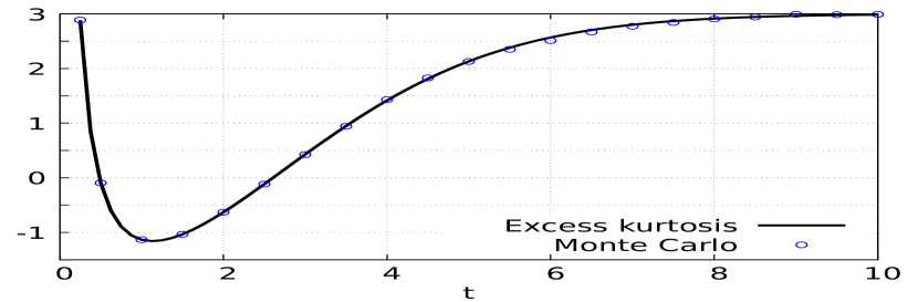
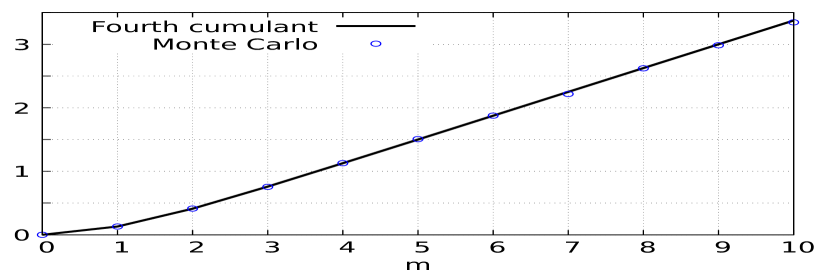
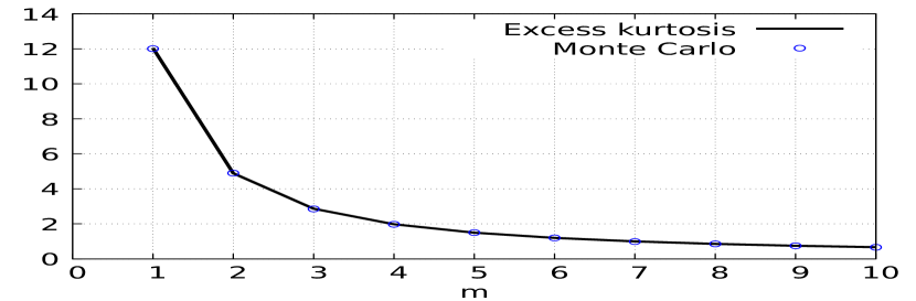
see Figure 5
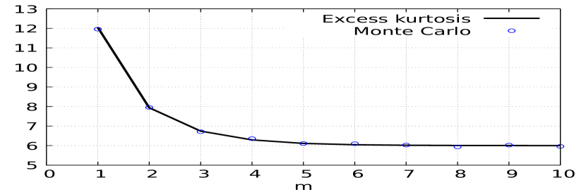
Figure 5 : Fourth cumulant and excess kurtosis of Y ( m ) 𝑌 𝑚 Y(m)
Compensated embedded chain
Finally, we consider the compensated embedded chain
X ( m ) 𝑋 𝑚 \displaystyle X(m) := assign \displaystyle:= Y T m − f m ( T m ) subscript 𝑌 subscript 𝑇 𝑚 subscript 𝑓 𝑚 subscript 𝑇 𝑚 \displaystyle Y_{T_{m}}-f_{m}(T_{m}) (6.6)
= \displaystyle= − f m ( T m ) + ∑ k = 1 m g ( T k , k , m ) subscript 𝑓 𝑚 subscript 𝑇 𝑚 superscript subscript 𝑘 1 𝑚 𝑔 subscript 𝑇 𝑘 𝑘 𝑚 \displaystyle-f_{m}(T_{m})+\sum_{k=1}^{m}g(T_{k},k,m)
= \displaystyle= − f m ( T m ) + ∑ k = 1 m f k ( s ) ( 1 − Z k ) ∏ l = k + 1 n Z l , m ≥ 1 , subscript 𝑓 𝑚 subscript 𝑇 𝑚 superscript subscript 𝑘 1 𝑚 subscript 𝑓 𝑘 𝑠 1 subscript 𝑍 𝑘 superscript subscript product 𝑙 𝑘 1 𝑛 subscript 𝑍 𝑙 𝑚
1 \displaystyle-f_{m}(T_{m})+\sum_{k=1}^{m}f_{k}(s)(1-Z_{k})\prod_{l=k+1}^{n}Z_{l},\qquad m\geq 1,
where ( Z k ) k ≥ 1 subscript subscript 𝑍 𝑘 𝑘 1 (Z_{k})_{k\geq 1} m n = 𝔼 [ Z n ] subscript 𝑚 𝑛 𝔼 delimited-[] superscript 𝑍 𝑛 m_{n}=\mathbb{E}[Z^{n}] n ≥ 0 𝑛 0 n\geq 0 6.1 g ( s , m , m ) = f m ( s ) ( 1 − Z m ) 𝑔 𝑠 𝑚 𝑚 subscript 𝑓 𝑚 𝑠 1 subscript 𝑍 𝑚 g(s,m,m)=f_{m}(s)(1-Z_{m}) g ( s , m , m ) = f m ( s ) ( 1 − Z m ) − f m ( s ) = − f m ( s ) Z m 𝑔 𝑠 𝑚 𝑚 subscript 𝑓 𝑚 𝑠 1 subscript 𝑍 𝑚 subscript 𝑓 𝑚 𝑠 subscript 𝑓 𝑚 𝑠 subscript 𝑍 𝑚 g(s,m,m)=f_{m}(s)(1-Z_{m})-f_{m}(s)=-f_{m}(s)Z_{m} 6.1 6.2 i = m − k 𝑖 𝑚 𝑘 i=m-k N s k = m − k subscript 𝑁 subscript 𝑠 𝑘 𝑚 𝑘 N_{s_{k}}=m-k LABEL:fjkldsf3 ),
by changing
the last term C q k − 1 , q k − q k − 1 subscript 𝐶 subscript 𝑞 𝑘 1 subscript 𝑞 𝑘 subscript 𝑞 𝑘 1
C_{q_{k-1},q_{k}-q_{k-1}} l = k 𝑙 𝑘 l=k ∏ l = 1 k C q l − 1 , q l − q l − 1 superscript subscript product 𝑙 1 𝑘 subscript 𝐶 subscript 𝑞 𝑙 1 subscript 𝑞 𝑙 subscript 𝑞 𝑙 1
\displaystyle\prod_{l=1}^{k}C_{q_{l-1},q_{l}-q_{l-1}} ( − 1 ) q k − q k − 1 m q k = ( − 1 ) q k − q k − 1 m n superscript 1 subscript 𝑞 𝑘 subscript 𝑞 𝑘 1 subscript 𝑚 subscript 𝑞 𝑘 superscript 1 subscript 𝑞 𝑘 subscript 𝑞 𝑘 1 subscript 𝑚 𝑛 (-1)^{q_{k}-q_{k-1}}m_{q_{k}}=(-1)^{q_{k}-q_{k-1}}m_{n}
Corollary 6.4
Let ( X ( m ) ) m ≥ 1 subscript 𝑋 𝑚 𝑚 1 (X(m))_{m\geq 1} 6.6 n , m ≥ 1 𝑛 𝑚
1 n,m\geq 1
𝔼 [ ( X ( m ) ) n ] = n ! ∑ k = 1 n ∑ i = 0 m − k − 1 λ k + i i ! m n m − i − k ∑ 0 = q 0 < q 1 < ⋯ < q k − 1 < q k = n 𝔼 delimited-[] superscript 𝑋 𝑚 𝑛 𝑛 superscript subscript 𝑘 1 𝑛 superscript subscript 𝑖 0 𝑚 𝑘 1 superscript 𝜆 𝑘 𝑖 𝑖 superscript subscript 𝑚 𝑛 𝑚 𝑖 𝑘 subscript 0 subscript 𝑞 0 subscript 𝑞 1 ⋯ subscript 𝑞 𝑘 1 subscript 𝑞 𝑘 𝑛 \displaystyle\mathbb{E}\big{[}(X(m))^{n}\big{]}=n!\sum_{k=1}^{n}\sum_{i=0}^{m-k-1}\frac{\lambda^{k+i}}{i!}m_{n}^{m-i-k}\sum_{0=q_{0}<q_{1}<\cdots<q_{k-1}<q_{k}=n}
∫ 0 ∞ e − λ s k ∫ 0 s k ⋯ ∫ 0 s 2 ( s 1 + ∑ l = 1 k − 1 m q l ( s l + 1 − s l ) ) i ∏ l = 1 k C q l − 1 , q l − q l − 1 f l , m q l − q l − 1 ( s l ) ( q l − q l − 1 ) ! d s 1 ⋯ d s k superscript subscript 0 superscript e 𝜆 subscript 𝑠 𝑘 superscript subscript 0 subscript 𝑠 𝑘 ⋯ superscript subscript 0 subscript 𝑠 2 superscript subscript 𝑠 1 superscript subscript 𝑙 1 𝑘 1 subscript 𝑚 subscript 𝑞 𝑙 subscript 𝑠 𝑙 1 subscript 𝑠 𝑙 𝑖 superscript subscript product 𝑙 1 𝑘 subscript 𝐶 subscript 𝑞 𝑙 1 subscript 𝑞 𝑙 subscript 𝑞 𝑙 1
superscript subscript 𝑓 𝑙 𝑚
subscript 𝑞 𝑙 subscript 𝑞 𝑙 1 subscript 𝑠 𝑙 subscript 𝑞 𝑙 subscript 𝑞 𝑙 1 𝑑 subscript 𝑠 1 ⋯ 𝑑 subscript 𝑠 𝑘 \displaystyle\int_{0}^{\infty}\mathrm{e}^{-\lambda s_{k}}\int_{0}^{s_{k}}\cdots\int_{0}^{s_{2}}\left(s_{1}+\sum_{l=1}^{k-1}m_{q_{l}}(s_{l+1}-s_{l})\right)^{i}\prod_{l=1}^{k}\frac{C_{q_{l-1},q_{l}-q_{l-1}}f_{l,m}^{q_{l}-q_{l-1}}(s_{l})}{(q_{l}-q_{l-1})!}ds_{1}\cdots ds_{k}
+ n ! ∑ k = 1 min ( n , m ) λ m ( m − k ) ! ∑ 0 = q 0 < q 1 < ⋯ < q k − 1 < q k = n ( − 1 ) q k − q k − 1 m n 𝑛 superscript subscript 𝑘 1 𝑛 𝑚 superscript 𝜆 𝑚 𝑚 𝑘 subscript 0 subscript 𝑞 0 subscript 𝑞 1 ⋯ subscript 𝑞 𝑘 1 subscript 𝑞 𝑘 𝑛 superscript 1 subscript 𝑞 𝑘 subscript 𝑞 𝑘 1 subscript 𝑚 𝑛 \displaystyle+n!\sum_{k=1}^{\min(n,m)}\frac{\lambda^{m}}{(m-k)!}\sum_{0=q_{0}<q_{1}<\cdots<q_{k-1}<q_{k}=n}(-1)^{q_{k}-q_{k-1}}m_{n}
∫ 0 ∞ e − λ s k f k , m n − q k − 1 ( s k ) ∫ 0 s k ⋯ ∫ 0 s 2 ( s 1 + ∑ l = 1 k − 1 m q l ( s l + 1 − s l ) ) m − k ∏ l = 1 k − 1 C q l − 1 , q l − q l − 1 f l , m q l − q l − 1 ( s l ) ( q l − q l − 1 ) ! d s 1 ⋯ d s k . superscript subscript 0 superscript e 𝜆 subscript 𝑠 𝑘 superscript subscript 𝑓 𝑘 𝑚
𝑛 subscript 𝑞 𝑘 1 subscript 𝑠 𝑘 superscript subscript 0 subscript 𝑠 𝑘 ⋯ superscript subscript 0 subscript 𝑠 2 superscript subscript 𝑠 1 superscript subscript 𝑙 1 𝑘 1 subscript 𝑚 subscript 𝑞 𝑙 subscript 𝑠 𝑙 1 subscript 𝑠 𝑙 𝑚 𝑘 superscript subscript product 𝑙 1 𝑘 1 subscript 𝐶 subscript 𝑞 𝑙 1 subscript 𝑞 𝑙 subscript 𝑞 𝑙 1
superscript subscript 𝑓 𝑙 𝑚
subscript 𝑞 𝑙 subscript 𝑞 𝑙 1 subscript 𝑠 𝑙 subscript 𝑞 𝑙 subscript 𝑞 𝑙 1 𝑑 subscript 𝑠 1 ⋯ 𝑑 subscript 𝑠 𝑘 \displaystyle\int_{0}^{\infty}\mathrm{e}^{-\lambda s_{k}}f_{k,m}^{n-q_{k-1}}(s_{k})\int_{0}^{s_{k}}\cdots\int_{0}^{s_{2}}\left(s_{1}+\sum_{l=1}^{k-1}m_{q_{l}}(s_{l+1}-s_{l})\right)^{m-k}\prod_{l=1}^{k-1}\frac{C_{q_{l-1},q_{l}-q_{l-1}}f_{l,m}^{q_{l}-q_{l-1}}(s_{l})}{(q_{l}-q_{l-1})!}ds_{1}\cdots ds_{k}.
Similarly, according to Corollary 6.3
X ( m ) = T m − ∑ k = 1 m T k ( 1 − U k ) ∏ l = k + 1 m U l , 𝑋 𝑚 subscript 𝑇 𝑚 superscript subscript 𝑘 1 𝑚 subscript 𝑇 𝑘 1 subscript 𝑈 𝑘 superscript subscript product 𝑙 𝑘 1 𝑚 subscript 𝑈 𝑙 X(m)=T_{m}-\sum_{k=1}^{m}T_{k}(1-U_{k})\prod_{l=k+1}^{m}U_{l}, (6.7)
with ( U k ) k ≥ 1 subscript subscript 𝑈 𝑘 𝑘 1 (U_{k})_{k\geq 1} ∏ l = 1 k 1 1 + q l superscript subscript product 𝑙 1 𝑘 1 1 subscript 𝑞 𝑙 \displaystyle\prod_{l=1}^{k}\frac{1}{1+q_{l}} i = m − k 𝑖 𝑚 𝑘 i=m-k LABEL:fjkldsf3-2 )
by
( − 1 ) q k − q k − 1 m q k C q k − 1 , q k − q k − 1 = ( − 1 ) q k − q k − 1 ( 1 + q k ) ! ( 1 + q k ) q k − 1 ! ( q k − q k − 1 ) ! = ( − 1 ) q k − q k − 1 ( n q k − 1 ) , superscript 1 subscript 𝑞 𝑘 subscript 𝑞 𝑘 1 subscript 𝑚 subscript 𝑞 𝑘 subscript 𝐶 subscript 𝑞 𝑘 1 subscript 𝑞 𝑘 subscript 𝑞 𝑘 1
superscript 1 subscript 𝑞 𝑘 subscript 𝑞 𝑘 1 1 subscript 𝑞 𝑘 1 subscript 𝑞 𝑘 subscript 𝑞 𝑘 1 subscript 𝑞 𝑘 subscript 𝑞 𝑘 1 superscript 1 subscript 𝑞 𝑘 subscript 𝑞 𝑘 1 binomial 𝑛 subscript 𝑞 𝑘 1 \frac{(-1)^{q_{k}-q_{k-1}}m_{q_{k}}}{C_{q_{k-1},q_{k}-q_{k-1}}}=\frac{(-1)^{q_{k}-q_{k-1}}(1+q_{k})!}{(1+q_{k})q_{k-1}!(q_{k}-q_{k-1})!}=(-1)^{q_{k}-q_{k-1}}{n\choose q_{k-1}},
as is done in the next corollary.
Corollary 6.5
Let ( X ( m ) ) m ≥ 1 subscript 𝑋 𝑚 𝑚 1 (X(m))_{m\geq 1} 6.7 ( U k ) k ≥ 1 subscript subscript 𝑈 𝑘 𝑘 1 (U_{k})_{k\geq 1} n , m ≥ 1 𝑛 𝑚
1 n,m\geq 1
𝔼 [ ( Y ( m ) ) n ] 𝔼 delimited-[] superscript 𝑌 𝑚 𝑛 \displaystyle\mathbb{E}\big{[}(Y(m))^{n}\big{]} = \displaystyle= ∑ k = 1 n ∑ i = 0 m − k − 1 λ k + i i ! ( n + 1 ) m − i − k ∑ 0 = q 0 < q 1 < ⋯ < q k − 1 < q k = n superscript subscript 𝑘 1 𝑛 superscript subscript 𝑖 0 𝑚 𝑘 1 superscript 𝜆 𝑘 𝑖 𝑖 superscript 𝑛 1 𝑚 𝑖 𝑘 subscript 0 subscript 𝑞 0 subscript 𝑞 1 ⋯ subscript 𝑞 𝑘 1 subscript 𝑞 𝑘 𝑛 \displaystyle\sum_{k=1}^{n}\sum_{i=0}^{m-k-1}\frac{\lambda^{k+i}}{i!(n+1)^{m-i-k}}\sum_{0=q_{0}<q_{1}<\cdots<q_{k-1}<q_{k}=n}
∫ 0 ∞ e − λ s k ∫ 0 s k ⋯ ∫ 0 s 2 ( s 1 + ∑ l = 1 k − 1 s l + 1 − s l 1 + q l ) i ∏ l = 1 k f l , m q l − q l − 1 ( s l ) 1 + q l d s 1 ⋯ d s k superscript subscript 0 superscript e 𝜆 subscript 𝑠 𝑘 superscript subscript 0 subscript 𝑠 𝑘 ⋯ superscript subscript 0 subscript 𝑠 2 superscript subscript 𝑠 1 superscript subscript 𝑙 1 𝑘 1 subscript 𝑠 𝑙 1 subscript 𝑠 𝑙 1 subscript 𝑞 𝑙 𝑖 superscript subscript product 𝑙 1 𝑘 superscript subscript 𝑓 𝑙 𝑚
subscript 𝑞 𝑙 subscript 𝑞 𝑙 1 subscript 𝑠 𝑙 1 subscript 𝑞 𝑙 𝑑 subscript 𝑠 1 ⋯ 𝑑 subscript 𝑠 𝑘 \displaystyle\quad\int_{0}^{\infty}\mathrm{e}^{-\lambda s_{k}}\int_{0}^{s_{k}}\cdots\int_{0}^{s_{2}}\left(s_{1}+\sum_{l=1}^{k-1}\frac{s_{l+1}-s_{l}}{1+q_{l}}\right)^{i}\prod_{l=1}^{k}\frac{f_{l,m}^{q_{l}-q_{l-1}}(s_{l})}{1+q_{l}}ds_{1}\cdots ds_{k}
+ ∑ k = 1 min ( n , m ) λ m ( m − k ) ! ∑ 0 = q 0 < q 1 < ⋯ < q k − 1 < q k = n ( − 1 ) q k − q k − 1 ( n q k − 1 ) superscript subscript 𝑘 1 𝑛 𝑚 superscript 𝜆 𝑚 𝑚 𝑘 subscript 0 subscript 𝑞 0 subscript 𝑞 1 ⋯ subscript 𝑞 𝑘 1 subscript 𝑞 𝑘 𝑛 superscript 1 subscript 𝑞 𝑘 subscript 𝑞 𝑘 1 binomial 𝑛 subscript 𝑞 𝑘 1 \displaystyle+\sum_{k=1}^{\min(n,m)}\frac{\lambda^{m}}{(m-k)!}\sum_{0=q_{0}<q_{1}<\cdots<q_{k-1}<q_{k}=n}(-1)^{q_{k}-q_{k-1}}{n\choose q_{k-1}}
∫ 0 ∞ e − λ s k ∫ 0 s k ⋯ ∫ 0 s 2 ( s 1 + ∑ l = 1 k − 1 s l + 1 − s l 1 + q l ) m − k ∏ l = 1 k f l , m q l − q l − 1 ( s l ) 1 + q l d s 1 ⋯ d s k . superscript subscript 0 superscript e 𝜆 subscript 𝑠 𝑘 superscript subscript 0 subscript 𝑠 𝑘 ⋯ superscript subscript 0 subscript 𝑠 2 superscript subscript 𝑠 1 superscript subscript 𝑙 1 𝑘 1 subscript 𝑠 𝑙 1 subscript 𝑠 𝑙 1 subscript 𝑞 𝑙 𝑚 𝑘 superscript subscript product 𝑙 1 𝑘 superscript subscript 𝑓 𝑙 𝑚
subscript 𝑞 𝑙 subscript 𝑞 𝑙 1 subscript 𝑠 𝑙 1 subscript 𝑞 𝑙 𝑑 subscript 𝑠 1 ⋯ 𝑑 subscript 𝑠 𝑘 \displaystyle\quad\int_{0}^{\infty}\mathrm{e}^{-\lambda s_{k}}\int_{0}^{s_{k}}\cdots\int_{0}^{s_{2}}\left(s_{1}+\sum_{l=1}^{k-1}\frac{s_{l+1}-s_{l}}{1+q_{l}}\right)^{m-k}\prod_{l=1}^{k}\frac{f_{l,m}^{q_{l}-q_{l-1}}(s_{l})}{1+q_{l}}ds_{1}\cdots ds_{k}.
When f l , m ( s ) = s subscript 𝑓 𝑙 𝑚
𝑠 𝑠 f_{l,m}(s)=s 6.5
𝔼 [ ( X ( m ) ) 2 ] = 1 λ 2 ( 2 − 4 ( 1 2 ) m + 2 ( 1 3 ) m ) 𝔼 delimited-[] superscript 𝑋 𝑚 2 1 superscript 𝜆 2 2 4 superscript 1 2 𝑚 2 superscript 1 3 𝑚 \mathbb{E}\big{[}(X(m))^{2}\big{]}=\frac{1}{\lambda^{2}}\left(2-4\left(\frac{1}{2}\right)^{m}+2\left(\frac{1}{3}\right)^{m}\right)
which recovers Theorem 7 in Boxma et al. ( 2006 )
Figure 6 : Third cumulant and skewness of X ( m ) 𝑋 𝑚 X(m)
Higher order moments of X ( m ) 𝑋 𝑚 X(m) 6.5 f l , m ( s ) = s subscript 𝑓 𝑙 𝑚
𝑠 𝑠 f_{l,m}(s)=s 3 3 3 4 4 4 6 7
Figure 7 : Fourth cumulant and kurtosis of X ( m ) 𝑋 𝑚 X(m)