Bayesian inference on the isospin splitting of nucleon effective mass from giant resonances in ²⁰⁸Pb

Abstract

From a Bayesian analysis of the electric dipole polarizability, the constrained energy of isovector giant dipole resonance, the peak energy of isocalar giant quadrupole resonance and the constrained energy of isocalar giant monopole resonance in ²⁰⁸Pb, we extract the isoscalar and isovector effective masses in nuclear matter at saturation density $\rho_{0}$ as $m_{s,0}^{\ast}/m=0.87_{-0.04}^{+0.04}$ and $m_{v,0}^{\ast}/m=0.78_{-0.05}^{+0.06}$ at $90\%$ confidence level. The obtained constraints on $m_{s,0}^{\ast}$ and $m_{v,0}^{\ast}$ lead to a positive isospin splitting of nucleon effective mass in asymmetric nuclear matter of isospin asymmetry $\delta$ at $\rho_{0}$ as $m_{n-p}^{*}/m=(0.20^{+0.15}_{-0.14})\delta$. In addition, the symmetry energy at the subsaturation density $\rho^{\ast}=0.05~{}\mathrm{fm}^{-3}$ is determined to be $E_{\mathrm{sym}}(\rho^{\ast})=16.7\pm 1.3$ MeV at $90\%$ confidence level.

I Introduction

The nucleon effective mass, which characterizes the momentum or energy dependence of single nucleon potential in nuclear medium, is crucial in nuclear physics and astrophysics Jeukenne et al. (1976); Mahaux et al. (1985); Jaminon and Mahaux (1989); Li and Chen (2015); Li et al. (2018). While various kinds of nucleon effective masses have been defined in nonrelativistic and relativistic approaches Mahaux et al. (1985); Jaminon and Mahaux (1989); Li and Chen (2015); Li et al. (2018); Chen et al. (2007); Li et al. (2008), here we focus on the total effective mass normally used in the nonrelativistic approach. In asymmetric nuclear matter, effective masses of neutrons and protons, $m_{n}^{\ast}$ and $m_{p}^{\ast}$, may be different due to the momentum dependence of the symmetry potential. The difference $m_{n-p}^{\ast}\equiv m_{n}^{\ast}-m_{p}^{\ast}$ is the so-called isospin splitting of nucleon effective mass, which plays an important role in many physical phenomena and questions in nuclear physics, astrophysics, and cosmology Li and Chen (2015); Li et al. (2018). For example, the $m_{n-p}^{\ast}$ affects the isospin dynamics in heavy-ion collisions  Li et al. (2004); Li and Chen (2005); Chen et al. (2005); Rizzo et al. (2005); Giordano et al. (2010); Feng (2012); Zhang et al. (2014); Xie and Zhang (2014), thermodynamic properties of asymmetric nuclear matter Behera et al. (2011); Xu et al. (2015); Xu (2015), and cooling of neutron stars Baldo et al. (2014).

Due to the limited isospin asymmetry in normal nuclei, the accurate determination of $m_{n-p}^{\ast}$ is rather difficult. Even the sign of $m_{n-p}^{\ast}$ remains a debated issue. For example, $m_{n-p}^{\ast}>0$ in neutron-rich matter at the nuclear saturation density $\rho_{0}\approx 0.16$ fm^-3 is favored by optical model analyses of nucleon-nucleus scattering data Li et al. (2015); Xu et al. (2010), Skyrme energy density functional (EDF) Zhang and Chen (2016) and transport model Kong et al. (2017) analyses of nuclear giant resonances, Brueckner-Hartree-Fock calculations Zuo et al. (1999, 2005); Ma et al. (2004); van Dalen et al. (2005), chiral effective theory Zhang et al. (2018); Holt et al. (2013, 2016) and an analysis of various constraints on the magnitude and density slope of symmetry energy Li and Han (2013), whereas the transport model analyses on single and/or double n/p ratio in heavy-ion collisions  Coupland et al. (2016); Morfouace et al. (2019) (but see Ref. Kong et al. (2015)) and an energy density functional study on nuclear electric dipole polarizability Malik et al. (2018) lead to opposite conclusions.

To understand these contradictive results and eventually determine the isospin splitting of nucleon effective mass needs not only the improvement of both theoretical models/calculations and experimental measurements, but also more sophisticated analysis approaches to quantifying the model uncertainties based on given experimental measurements. The latter is a quite general issue in nuclear theory, where due to the lack of a well-settled ab initio starting point, a lot of effective theories or models have been developed with parameters determined by fitting empirical knowledge or experimental data Dobaczewski et al. (2014). Over the past decade, various statistical approaches, e.g., covariance analysis Reinhard and Nazarewicz (2010); Piekarewicz et al. (2015), Bayesian analysis McDonnell et al. (2015); Bernhard et al. (2015); Pratt et al. (2015); Xie and Li (2019, 2020); Drischler et al. (2020); Xu et al. (2020); Kejzlar et al. (2020) and bootstrap method Bertsch and Bingham (2017); Pastore (2019), have been introduced in nuclear physics studies to quantify uncertainties and evaluate correlations of model parameters. Among them, the Bayesian inference method has been accepted as a powerful statistical approach and extensively used in various areas of nuclear physics. For a very recent review on Bayesian analysis and its applications in nuclear structure study, we refer the readers to Ref. Kejzlar et al. (2020).

In our previous work Zhang and Chen (2016), we have extracted the isospin splitting of nucleon effective mass from the isovector giant dipole resonance (IVGDR) and isocalar giant quadrupole resonance (ISGQR) of ²⁰⁸Pb based on random phase approximation (RPA) calculations using a number of representative Skyrme interactions. However, some factors in the analysis, e.g., the choice of Skyrme interactions and the priorly assumed linear $1/E_{\mathrm{GQR}}^{2}$-$m_{s,0}^{\ast}$ relations, could affect the conclusions, and the statistical meaning of the obtained uncertainties are therefore unclear. In the present work, within the framework of Skyrme energy density functional theory and random phase approximation approach, we employ the Bayesian inference method to extract the isospin splitting of nucleon effective mass from the electric dipole polarizability Tamii et al. (2011); Roca-Maza et al. (2015), the constrained energy in IVGDR Dietrich and Berman (1988) and the ISGQR peak energy Roca-Maza et al. (2013a) in ²⁰⁸Pb. The binding energy Wang et al. (2017), the charge radius Angeli and Marinova (2013), the constrained energy of isocalar giant monopole resonance (ISGMR) Patel et al. (2013) and the neutron $3p_{1/2}-3p_{3/2}$ energy splitting Vautherin and Brink (1972) of ²⁰⁸Pb are also included in the analysis to guarantee the energy density functional can always reasonably describe the ground state and collective excitation state of ²⁰⁸Pb. The isoscalar and isovector effective masses, and the neutron-proton effective mass splitting at saturation density together with the symmetry energy at the subsaturation density $\rho^{\ast}=0.05~{}\mathrm{fm}^{-3}$ are extracted from the Bayesian analysis.

The paper is organized as follows. In Sec. II, we introduce the theoretical models and statistical approaches used in this work. In the next section presented are the results for the uncertainties of model parameters, the isospin splitting of nucleon effective mass at $\rho_{0}$ and the symmetry energy at $\rho^{\ast}=0.05~{}\mathrm{fm}^{-3}$. Finally, we draw conclusions in Sec. IV.

II Model and Method

II.1 Nucleon effective mass in Skyrme energy density functional

As in Ref. Zhang and Chen (2016), we study the nucleon effective mass within the standard Skyrme energy density functional based on the conventional Skyrme interaction:

$$v(\bm{r}_{1},\bm{r}_{2}) = t_{0}(1+x_{0}P_{\sigma})\delta(\bm{r}_{1}-\bm{r}_{2})$$ (1)

$$+\frac{1}{2}t_{1}(1+x_{1}P_{\sigma})[\bm{k}^{\prime 2}\delta(\bm{r}_{1}-\bm{r}_{2})+\mathrm{c.c.}]$$

$$+t_{2}(1+x_{2}P_{\sigma})\bm{k}^{\prime}\cdot\delta(\bm{r}_{1}-\bm{r}_{2})\bm{k}$$

$$+\frac{1}{6}t_{3}(1+x_{3}P_{\sigma})\rho^{\alpha}\left(\frac{\bm{r}_{1}+\bm{r}_{2}}{2}\right)\delta(\bm{r}_{1}-\bm{r}_{2})$$

$$+iW_{0}(\bm{\sigma}_{1}+\bm{\sigma}_{2})\cdot[\bm{k}^{\prime}\times\delta(\bm{r}_{1}-\bm{r}_{2})\bm{k}].$$

Here $\bm{\sigma}_{i}$ is the Pauli spin operator, $P_{\sigma}=(1+\bm{\sigma}_{1}\cdot\bm{\sigma}_{2})/2$ is the spin-exchange operator, $\bm{k}=-i(\bm{\nabla}_{1}-\bm{\nabla}_{2})/2$ is the relative momentum operator, and $\bm{k}^{\prime}$ is the conjugate operator of $\bm{k}$ acting on the left.

Within the framework of Skyrme energy density functional, the 9 parameters $t_{0}-t_{3}$, $x_{0}-x_{3}$ and $\alpha$ of the Skyrme interaction can be expressed in terms of 9 macroscopic quantities (pseudo-observables): the nuclear saturation density $\rho_{0}$, the energy per particle of symmetric nuclear matter $E_{0}(\rho_{0})$, the incompressibility $K_{0}$, the isocalar effective mass $m_{s,0}^{*}$ at $\rho_{0}$, the isovector effective mass $m_{v,0}^{*}$ at $\rho_{0}$, the gradient coefficient $G_{S}$, the symmetry-gradient coefficient $G_{V}$, and the magnitude $E_{\mathrm{sym}}(\rho_{0})$ and density slope $L$ of the nuclear symmetry energy at $\rho_{0}$ Chen et al. (2010); Chen and Gu (2012); Kortelainen et al. (2010). The detailed analytical expressions can be found in Ref. Chen et al. (2010); Chen and Gu (2012). Since the 9 macroscopic quantities have clear physical meaning and available empirical ranges, in the Bayesian analysis, we use them as model parameters. Consequently, our model has the following 10 parameters:

$$\bm{p} = \{\rho_{0},~{}E_{0}(\rho_{0}),~{}K_{0},~{}E_{\mathrm{sym}}(\rho_{0}),~{}L,$$ (2)

$$~{}G_{S},~{}G_{V},~{}W_{0},~{}m_{s,0}^{\ast},~{}m_{v,0}^{\ast}\}.$$

In terms of the Skyrme parameter $t_{0}\sim t_{3}$ and $x_{0}\sim x_{3}$, the nucleon effective mass in asymmetric nuclear matter with density $\rho$ and isospin asymmetry $\delta$ can be expressed as Chabanat et al. (1997)

$$\frac{\hbar^{2}}{2m_{q}^{\ast}(\rho,\delta)} = \frac{\hbar^{2}}{2m}+\frac{1}{4}t_{1}\left[\left(1+\frac{1}{2}x_{1}\right)\rho-\left(\frac{1}{2}+x_{1}\right)\rho_{q}\right]$$ (3)

$$+ \frac{1}{4}t_{2}\left[\left(1+\frac{1}{2}x_{2}\right)\rho+\left(\frac{1}{2}+x_{2}\right)\rho_{q}\right].$$

The well-known isocalar and isovector effective masses, $m_{s}^{\ast}$ and $m_{v}^{\ast}$, which are respectively defined as the proton (neutron) effective mass in symmetric nuclear matter and pure neutron (proton) matter, are then given by Chabanat et al. (1997)

$$\frac{\hbar^{2}}{2m_{s}^{\ast}(\rho)}=\frac{\hbar^{2}}{2m}+\frac{3}{16}t_{1}\rho+\frac{1}{16}t_{2}(4x_{2}+5)\rho,$$ (4)

$$\frac{\hbar^{2}}{2m_{v}^{*}(\rho)}=\frac{\hbar^{2}}{2m}+\frac{1}{8}t_{1}(x_{1}+2)\rho+\frac{1}{8}t_{2}(x_{2}+2)\rho.$$ (5)

Once given $m_{s}^{\ast}$ and $m_{v}^{\ast}$, the isospin splitting of nucleon effective mass can be obtained as Zhang and Chen (2015)

$$m^{\ast}_{n-p}(\rho,\delta) \equiv \frac{m_{n}^{\ast}-m_{p}^{\ast}}{m}=2\frac{m_{s}^{\ast}}{m}\sum_{n=1}^{\infty}\left(\frac{m_{s}^{\ast}-m_{v}^{\ast}}{m_{v}^{\ast}}\delta\right)^{2n-1}$$ (6)

$$= \sum_{n=1}^{\infty}\Delta m^{*}_{2n-1}(\rho)\delta^{2n-1},$$

with the isospin splitting coefficients $\Delta m^{*}_{2n-1}(\rho)$ given by

$$\Delta m^{*}_{2n-1}(\rho)=2\frac{m_{s}^{\ast}}{m}\left(\frac{m_{s}^{\ast}}{m_{v}^{\ast}}-1\right)^{2n-1}.$$ (7)

In the following, we use $\Delta m_{1}^{\ast}$ to indicate the linear isospin splitting coefficient at the saturation density $\rho_{0}$.

II.2 Nuclear giant resonances

Nuclear giant resonances are usually studied using random phase approximation (RPA) approach Colò et al. (2013). For a given excitation operator $\hat{F}_{JM}$, the strength function is calculated as:

$$S(E)=\sum_{\nu}|\langle\nu\|\hat{F}_{J}\|\tilde{0}\rangle|^{2}\delta(E-E_{\nu}),$$ (8)

with $E_{\nu}$ being the energy of RPA excitation state $|\nu\rangle$, and the moments $m_{k}$ of strength function (sum rules) are usually evaluated as:

$$m_{k}=\int dEE^{k}S(E)=\sum_{\nu}|\langle\nu\|\hat{F}_{J}\|\tilde{0}\rangle|^{2}E_{\nu}^{k}.$$ (9)

For the ISGMR, IVGDR and ISGQR studied here, the excitation operators are defined as:

$$\hat{F}^{\mathrm{IS}}_{0} = \sum_{i}^{A}r_{i}^{2}$$ (10)

$$\hat{F}^{\mathrm{IV}}_{1M} = \frac{N}{A}\sum^{Z}_{i=1}r_{i}Y_{\text{1M}}(\hat{r}_{i})-\frac{Z}{A}\sum^{N}_{i=1}r_{i}Y_{\text{1M}}(\hat{r}_{i}),$$ (11)

$$\hat{F}^{\mathrm{IS}}_{2M} = \sum_{i=1}^{A}r_{i}^{2}Y_{2M}(\hat{r}_{i}),$$ (12)

where $Z$, $N$ and $A$ are proton, neutron and mass number, respectively; $r_{i}$ is the nucleon’s radial coordinate; $Y_{\text{1M}}(\hat{r_{i}})$ and $Y_{\text{2M}}(\hat{r_{i}})$ are the corresponding spherical harmonic function.

Particularly, in linear response theory, the inverse energy weighted sum rule can also be extracted from the constrained Hartree-Fock (CHF) approach Bohigas et al. (1979); Sil et al. (2006):

$$m_{-1}=-\left.\frac{1}{2}\frac{d^{2}\langle\lambda|\mathcal{H}|\lambda\rangle}{d\lambda^{2}}\right|_{\lambda=0},$$ (13)

where $|\lambda\rangle$ is the ground-state for the nuclear system Hamilton $\mathcal{H}$ constrained by the field $\lambda\hat{F}_{J}$.

The energy of isoscalar giant monopole resonance (GMR), i.e., the breathing mode, is an important probe of the incompressibility in nuclear matter. It can be evaluated in the constrained approximation Blaizot (1980) as

$$E_{\mathrm{GMR}}=\sqrt{\frac{m_{1}(\mathrm{GMR})}{m_{-1}(\mathrm{GMR})}},$$ (14)

where the energy weighted sum rule $m_{1}$ of ISGMR is related to the ground-state rms radius $\langle r^{2}\rangle$ by Bohr and Mottelson (1975)

$$m_{1}(\mathrm{GMR})=2\frac{\hbar^{2}}{m}A\langle r^{2}\rangle.$$ (15)

Therefore, we calculate the $E_{\mathrm{GMR}}$ by using the CHF method for computational efficiency.

For the isovector giant dipole resonance, we consider two observables, the electric dipole polarizability $\alpha_{\mathrm{D}}$ and the constrained energy $E_{\mathrm{GDR}}\equiv\sqrt{m_{1}/m_{-1}}$. The $\alpha_{\mathrm{D}}$ in ²⁰⁸Pb probes the symmetry energy at about $\rho_{0}/3$ Zhang and Chen (2015) and is therefore sensitive to both the magnitude and density slope of the symmetry energy at saturation density Roca-Maza et al. (2013b). It is related to the inverse energy-weighted sum rule in the IVGDR by

$$\alpha_{\mathrm{D}}=\frac{8\pi}{9}e^{2}m_{-1}(\mathrm{GDR}).$$ (16)

Meanwhile, the energy weighted sum rule $m_{1}$ of IVGDR is related to the isovector effective mass at saturation density $m_{v,0}^{\ast}$ via Colò et al. (2013); Zhang and Chen (2016)

$$m_{1}(\mathrm{GDR})=\frac{9}{4\pi}\frac{\hbar^{2}}{2m}\frac{NZ}{A}(1+\kappa)\approx\frac{9\hbar^{2}}{8\pi}\frac{NZ}{A}\frac{1}{m_{v,0}^{\ast}},$$ (17)

where $\kappa$ is the well-known Thomas-Reiche-Kuhn sum rule enhancement. One then has approximately

$$~{}E_{\mathrm{GDR}}^{2}\propto\frac{1}{m_{v,0}^{\ast}\alpha_{\mathrm{D}}},$$ (18)

which suggests that the $E_{\mathrm{GDR}}$ is negatively correlated to the $m_{v,0}^{\ast}$.

As well known, the excitation energy of isocalar giant quadruple resonance is sensitive to the isoscalar effective mass at saturation density. For example in the harmonic oscillator model, the ISGQR energy is Bohr and Mottelson (1975); Roca-Maza et al. (2013a)

$$E_{\mathrm{GQR}}=\sqrt{\frac{2m}{m_{s,0}^{*}}}\hbar\omega_{0}$$ (19)

with $\hbar\omega_{0}$ being the frequency of the harmonic oscillator. In the present work, we determine the $E_{\mathrm{GQR}}$ as the peak energy of the response function obtained from RPA calculations. To obtain continuous response function, the discrete RPA results are smeared out with Lorentzian functions. The width of Lorentzian functions is taken to be $3$ MeV to roughly reproduce experimental width $\sim 3$ MeV of ISGQR.

Table 1: Prior ranges of the ten parameters used.

Quantity	lower limit	upper limit
$\rho_{0}~{}(\mathrm{fm}^{-3})$	0.155	0.165
$E_{0}~{}(\mathrm{MeV})$	-16.5	-15.5
$K_{0}~{}(\mathrm{MeV})$	210.0	250.0
$E_{\mathrm{sym}}(\rho_{0})~{}(\mathrm{MeV})$	29.0	35.0
$L~{}(\mathrm{MeV})$	20.0	120.0
$G_{S}~{}(\mathrm{MeV}\cdot\mathrm{fm}^{5})$	110.0	170.0
$G_{V}~{}(\mathrm{MeV}\cdot\mathrm{fm}^{5})$	-70.0	70.0
$W_{0}~{}(\mathrm{MeV}\cdot\mathrm{fm}^{5})$	110.0	140.0
$m_{s,0}^{\ast}/m$	0.7	1.0
$m_{v,0}^{\ast}/m$	0.6	0.9

Table 2: Experimental values and uncertainties used for the binding energy $E_{B}$ Wang et al. (2017), the charge radius $r_{C}$ Angeli and Marinova (2013), the breathing mode energy $E_{\mathrm{GMR}}$ Patel et al. (2013), the neutron $3p_{1/2}-3p_{3/2}$ energy level splitting $\epsilon_{ls}$ Vautherin and Brink (1972), the electric dipole polarizability $\alpha_{\mathrm{D}}$ Tamii et al. (2011); Roca-Maza et al. (2015), the IVGDR constrained energy Dietrich and Berman (1988) and the ISGQR peak energy Roca-Maza et al. (2013a) in ²⁰⁸Pb.

	value	$\sigma$
$E_{B}$ (MeV)	-1363.43	0.5
$r_{C}$ (fm)	5.5012	0.01
$E_{\mathrm{GMR}}$ (MeV)	13.5	0.1
$\epsilon_{ls}$ (MeV)	0.89	0.09
$\alpha_{\mathrm{D}}~{}(\mathrm{fm}^{3})$	19.6	0.6
$E_{\mathrm{GDR}}$ (MeV)	13.46	0.1
$E_{\mathrm{GQR}}$ (MeV)	10.9	0.1

II.3 Bayesian analysis

The Bayesian analysis method has been widely accepted as a powerful statistical approach to quantifying the uncertainties and evaluating the correlations of model parameters as well as making predictions with certain confidence level according to experimental measurements and empirical knowledge McDonnell et al. (2015); Bernhard et al. (2015); Pratt et al. (2015); Xie and Li (2019, 2020); Drischler et al. (2020); Xu et al. (2020); Kejzlar et al. (2020). In this work, we employ the MADAI package MAD to do Bayesian analysis based on the Gaussian process emulators. For details on the statistical approach, we refer the readers to, e.g., Ref. Bernhard et al. (2015).

According to Bayes’ theorem, the posterior probability distribution of model parameter $\bm{p}$ (which we are seeking for) given experimental measurements $\bm{\mathcal{O}}^{\mathrm{exp}}$ for a set of observables $\bm{\mathcal{O}}$ can be evaluated as

$$P(\bm{p}|\mathcal{M},\bm{\mathcal{O}}^{\mathrm{exp}})=\frac{P(\mathcal{M},\bm{\mathcal{O}}^{\mathrm{exp}}\mid\bm{p})P(\bm{p})}{\int P(\mathcal{M},\bm{\mathcal{O}}^{\mathrm{exp}}\mid\bm{p})P(\bm{p})d\bm{p}},$$ (20)

where $\mathcal{M}$ is the given model, $P(\bm{p})$ is the prior probability of model parameters $\bm{p}$ before being confronted with the experimental measurements $\bm{\mathcal{O}}^{\mathrm{exp}}$, and $P(\mathcal{M},\bm{\mathcal{O}}^{\mathrm{exp}}|\bm{p})$ denotes the likelihood or the conditional probability of observing $\bm{\mathcal{O}}^{\mathrm{exp}}$ given the model $\mathcal{M}$ predictions at $\bm{p}$. The posterior univariate distribution of a single model parameter $p_{i}$ is given by

$$P(p_{i}|\mathcal{M},\bm{\mathcal{O}}^{\mathrm{exp}})=\frac{\int P(\bm{p}|\mathcal{M},\bm{\mathcal{O}}^{\mathrm{exp}})d\prod_{j\neq i}p_{j}}{\int P(\bm{p}|\mathcal{M},\bm{\mathcal{O}}^{\mathrm{exp}})d\prod_{j}p_{j}},$$ (21)

and the correlated bivariate distribution of two parameters $p_{i}$ and $p_{j}$ is given by

$$P[(p_{i},p_{j})|\mathcal{M},\bm{\mathcal{O}}^{\mathrm{exp}}]=\frac{\int P(\bm{p}|\mathcal{M},\bm{\mathcal{O}}^{\mathrm{exp}})d\prod_{k\neq i,j}p_{k}}{\int P(\bm{p}|\mathcal{M},\bm{\mathcal{O}}^{\mathrm{exp}})d\prod_{k}p_{k}}.$$ (22)

From the univariate distribution, the mean value of $p_{i}$ can be calculated as

$$\langle p_{i}\rangle=\int p_{i}P(p_{i}|\mathcal{M},\bm{\mathcal{O}}^{\mathrm{exp}})dp_{i}.$$ (23)

The confidence interval of $p_{i}$ at a confidence level $1-\alpha$ is normally obtained as the interval between the $(50\alpha)^{\text{th}}$ and $(100-50\alpha)^{\text{th}}$ percentile of the posterior univariate distribution. Particularly, the median value $U_{p_{i}}$ of $p_{i}$ is defined as the $50^{\mathrm{th}}$ percentile, i.e.,

$$\int^{U_{p_{i}}}_{-\infty}P(p_{i}|\mathcal{M},\bm{\mathcal{O}}^{\mathrm{exp}})dp_{i}=0.5.$$ (24)

For the prior distribution, we assume the ten parameters uniformly distributed in the empirical ranges listed in Tab. 1. As can be seen from Eq. (20), the posterior distribution is determined by the combination of the prior distribution and likelihood function, which depends on the experimental measurement for observable. Therefore, the prior distribution is very important in the Bayesian analysis and can significantly affect the extracted constraints. Nevertheless, in the present work, due to the relatively poor knowledge on $m_{s,0}^{\ast}$ and $m_{v,0}^{\ast}$ in the Skyrme EDF, we assume large prior ranges for $m_{s,0}^{\ast}$ and $m_{v,0}^{\ast}$ and thus the constraints on nucleon effective masses are mainly due to the giant resonance observables. Narrowing the prior ranges of all parameters by $20\%$ only slightly reduces the posterior uncertainties of the iospin splitting of nucleon effective mass by few percent.

The likelihood function is taken to be the commonly used Gaussian form

$$P(\mathcal{M},\bm{\mathcal{O}}^{\mathrm{exp}}_{i}\mid\bm{p})\propto\mathrm{exp}\left\{-\sum_{i}\frac{[\mathcal{O}_{i}(\bm{p})-\mathcal{O}^{\mathrm{exp}}_{i}]^{2}}{2\sigma_{i}^{2}}\right\},$$ (25)

where $\mathcal{O}_{i}(\bm{p})$ is the model prediction for an observable at given point $\bm{p}$, $\mathcal{O}^{\mathrm{exp}}_{i}$ is the corresponding experimental measurement, and $\sigma_{i}$ is the uncertainty or the width of likelihood function. For a given parameter set $\bm{p}$, we calculate the following 7 observables in ²⁰⁸Pb from Hartree-Fock, CHF and RPA calculations: the electric dipole polarizability $\alpha_{\rm{D}}$ Tamii et al. (2011); Roca-Maza et al. (2015), the IVGDR constrained energy $E_{\rm{GDR}}$Dietrich and Berman (1988), the ISGQR peak energy $E_{\mathrm{GQR}}$ Roca-Maza et al. (2013a), the binding energy $E_{B}$ Wang et al. (2017), the charge radius $r_{C}$ Angeli and Marinova (2013), the breathing mode energy $E_{\mathrm{GMR}}$ Patel et al. (2013) and the neutron $3p_{1/2}-3p_{3/2}$ energy level splitting $\epsilon_{ls}$ Vautherin and Brink (1972). The experimental values for the 7 observables together with the assigned uncertainties are listed in Tab. 2. For the $\alpha_{\mathrm{D}}$ and $E_{\mathrm{GMR}}$, the $\sigma_{i}$ are taken to be their experimental uncertainties given in Refs. Tamii et al. (2011) and Patel et al. (2013); for the well determined $E_{B}$, $r_{C}$, $\epsilon_{ls}$ and $E_{\mathrm{GDR}}$, we assign them artificial $1\sigma$ errors of $0.5$ MeV, $0.01$ fm, $0.09$ MeV and $0.1$ MeV, respectively; for the experimental value and uncertainty of $E_{\mathrm{GQR}}$, we use the weighted average of experimental measurements, $10.9\pm 0.1$ MeV reported in Ref. Roca-Maza et al. (2013a). We note that decreasing the artificial errors of $E_{B}$, $r_{C}$, $\epsilon_{ls}$ and $E_{\mathrm{GDR}}$ by half only slightly reduces the posterior uncertainty of $\Delta m_{1}^{*}$ by about $7\%$, and does not affect the constraint on the symmetry energy at the subsaturation density $\rho^{*}=0.05~{}\mathrm{fm}^{-3}$.

According to the prior distribution and defined likelihood function, the Markov chain Monte Carlo (MCMC) process using Metropolis-Hastings algorithm is performed to evaluate the posterior distributions of model parameters. For 10-dimensional parameter space in this work, a huge number of MCMC steps are needed to extract posterior distributions, and thus theoretical calculations for all MCMC steps are infeasible. Instead, in this work, we first sample a number of parameter sets in the designed parameter space, and train Gaussian process (GP) emulators Rasmussen and Williams (2006) using the model predictions with the sampled parameter sets. The obtained GPs provide fast interpolators and are used to evaluate the likelihood function in each MCMC step.

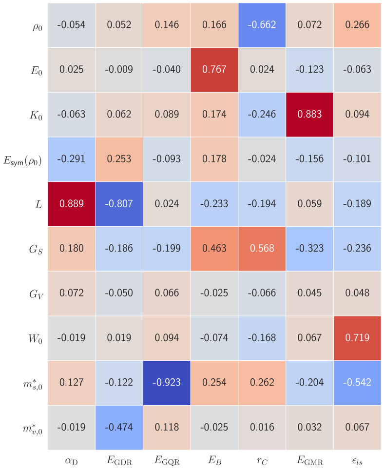
Figure 1: (Color online). Visualization of the Pearson correlation coefficients among model parameters and observables from the training data. The numerical values of correlation coefficients are annotated and color-coded, where darker red indicates more positive values and darker blue indicates more negative.

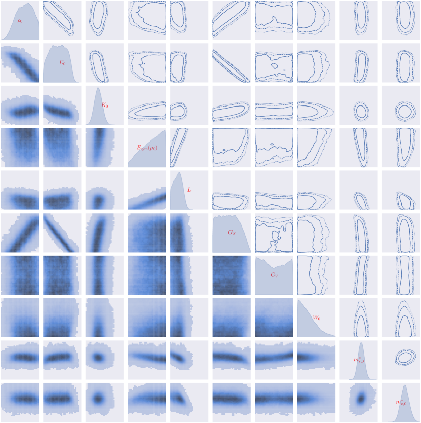
Figure 2: (Color online). Univariate and bivariate posterior distributions of the 10 model parameters. The solid, dashed and dotted lines in the upper-right panels enclose $68.3\%$, $90\%$ and $95.4\%$ confidence regions, respectively; the diagonal plots show Gaussian kernel density estimations of the posterior marginal distribution for respective parameters; in the lower-left panels are scatter histograms of MCMC samples. The range of variations of the 10 parameters are the prior range listed in Table 1.

Table 3: Best value, mean, median and confidence intervals of the model parameters from MCMC sampling.

	best	mean	median	$68.3\%$ C.I.	$90\%$ C.I.	$95.4\%$ C.I.
$\rho_{0}~{}(\text{fm}^{-3})$	0.1597	0.1612	0.1613	$0.1589\sim 0.1635$	$0.1577\sim 0.1644$	$0.1570\sim 0.1647$
$E_{0}~{}(\text{MeV})$	-16.04	-16.10	-16.10	$-16.34\sim-15.87$	$-16.44\sim-15.78$	$-16.47\sim-15.74$
$K_{0}~{}(\text{MeV})$	224.6	223.5	223.4	$219.4\sim 227.6$	$216.9\sim 230.3$	$215.6\sim 231.8$
$E_{\text{sym}}(\rho_{0})~{}(\text{MeV})$	34.4	32.7	33.0	$30.9\sim 34.4$	$29.9\sim 34.8$	$29.5\sim 34.9$
$L(\rho_{0})~{}(\text{MeV})$	48.8	40.3	40.4	$27.9\sim 51.9$	$22.8\sim 58.1$	$21.4\sim 61.1$
$G_{S}~{}(\text{MeV}\cdot\text{fm}^{5})$	125.7	135.5	135.1	$118.2\sim 152.5$	$112.7\sim 160.3$	$111.2\sim 163.5$
$G_{V}~{}(\text{MeV}\cdot\text{fm}^{5})$	65.0	-1.6	-3.1	$-50.9\sim 49.5$	$-64.1\sim 63.9$	$-67.3\sim 67.3$
$W_{0}~{}(\text{MeV}\cdot\text{fm}^{5})$	111.6	118.4	117.0	$112.0\sim 125.1$	$110.6\sim 131.4$	$110.3\sim 134.7$
$m_{s,0}^{*}/m$	0.88	0.87	0.87	$0.84\sim 0.89$	$0.83\sim 0.91$	$0.82\sim 0.92$
$m_{v,0}^{*}/m$	0.78	0.78	0.78	$0.75\sim 0.81$	$0.73\sim 0.84$	$0.72\sim 0.85$

III Results and Discussions

We first generated 2500 parameter sets using the maximin Latin cube sampling method Morris and Mitchell (1995). 24 of them are near the edge of the allowed parameter space and lead to numerical instability in Hartree-Fock (HF) or RPA calculations. Therefore, we discarded the 24 parameter sets and used the left 2476 parameter sets in HF, CHF and RPA calculation to obtain the training data for Gaussian emulators.

Results from the 2476 training points can inform us of correlations between observables and model parameters. We show in Fig. 1 the Pearson correlation coefficients among model parameters and the chosen 7 observables obtained from the training data. In Fig. 1, darker red indicates positive larger value and thus stronger positive correlation, and darker blue indicates more negative value and thus stronger negative correlation. One can expect that the parameters strongly correlated with the chosen observables are more likely to be constrained. Particularly, it is seen that the correlations among observables in nuclear giant resonances and model parameters are nicely consistent with the empirical knowledge introduced in Chapter II.2: the $\alpha_{\mathrm{D}}$ is positively (negatively) correlated to $L$ [$E_{\mathrm{sym}}(\rho_{0})$] because it is mostly sensitive to the symmetry energy at $\rho^{\ast}=0.05~{}\mathrm{fm}^{-3}$ Zhang and Chen (2015); the $E_{\mathrm{GDR}}$ is negatively correlated to both $m_{v,0}^{\ast}$ and $L$, but positively to $E_{\mathrm{sym}}(\rho_{0})$, which can be understood from Eq. (18) and the dependence of $\alpha_{\mathrm{D}}$ on $L$ and $E_{\mathrm{sym}}(\rho_{0})$; the $E_{\mathrm{GQR}}$ is strongly negatively correlated with $m_{s,0}^{\ast}$ [see Eq. (19)]; the $E_{\mathrm{GMR}}$ is mostly sensitive to the incompressibility $K_{0}$. Meanwhile, the $G_{V}$ is weakly correlated to all observables, and therefore can not be well constrained in the present analysis.

Based on the training data, Gaussian process emulators were tuned to quickly predict model output for MCMC process. With the help of GPs, we first ran $10^{6}$ burn-in MCMC steps to allow the chain to reach equilibrium, and then generated $10^{7}$ points in parameter space via the MCMC sampling. The posterior distributions of model parameters are then extracted from the $10^{7}$ samples, and visualized in Fig. 2. The lower-left panels show the bivariate scatter histograms of the MCMC samples; the diagonal ones present the univariate posterior distribution of the model parameters; the solid, dashed, and dotted lines in the upper-right panels enclose $68.3\%$, $90\%$ and $95.4\%$ confidence regions, respectively. Fig. 2 intuitively present the uncertainties and correlations of the model parameter imposed by the experimental measurements for the chosen observables. Remarkably, $K_{0}$, $m_{s,0}^{\ast}$, and $m_{v,0}^{\ast}$ are well constrained by the giant monopole, dipole and quadruple resonances, respectively. Another interesting feature is the strong positive correlation between $E_{\mathrm{sym}}(\rho_{0})$ and $L$, which can be understood by the fact that $\alpha_{\mathrm{D}}$ is positively correlated to $L$ but negative to $E_{\mathrm{sym}}(\rho_{0})$ (see Fig. 1). Similarly, the $E_{B}$ datum leads to a negative $E_{0}$-$G_{S}$ correlation, and $r_{C}$ datum results in a positive $\rho_{0}$-$G_{S}$ correlation. Therefore, the combination of $E_{B}$ and $r_{C}$ leads to a negative $\rho_{0}$-$E_{0}$ correlation.

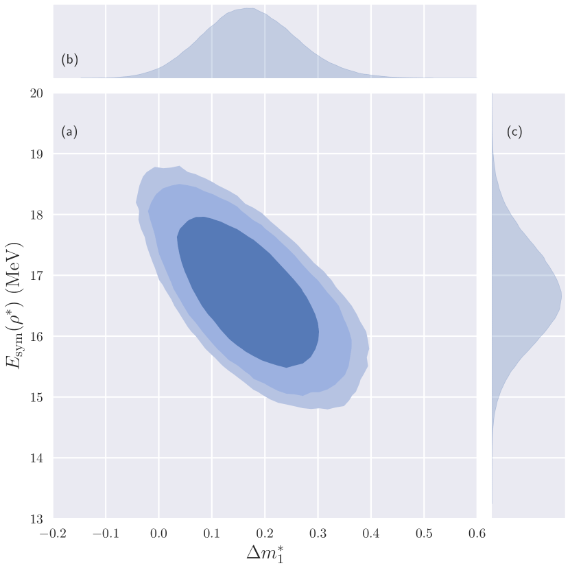
Figure 3: (Color online). Posterior bivariate (a) and univariate [(b) and (c)] distributions of $E_{\mathrm{sym}}(\rho^{\ast})$ at $\rho^{\ast}=0.05~{}\mathrm{fm}^{-3}$ and the linear isospin splitting coefficient $\Delta m_{1}^{\ast}$ at $\rho_{0}$. The shaded regions in window (a) indicate the $68.3\%$, $90\%$ and $95.4\%$ confidence regions.

To quantify the posterior distribution from the Bayesian analysis, we list statistical quantities estimated from the MCMC samples, including the mean value, median value and confidence intervals at $68.3\%$, $90\%$ and $95.4\%$ confidence levels. The best value, i.e., the parameter set that gives the largest likelihood function, is also listed for reference. In particular, we obtain $m_{s,0}^{\ast}/m=0.87_{-0.03}^{+0.02}$ and $m_{v,0}^{\ast}/m=0.78_{-0.03}^{+0.03}$ at $68\%$ confidence level, and $m_{s,0}^{\ast}/m=0.87_{-0.04}^{+0.04}$ and $m_{v,0}^{\ast}/m=0.78_{-0.05}^{+0.06}$ at $90\%$ confidence level. The results are consistent with $m_{s,0}^{\ast}=0.91\pm 0.05$ and $m_{v,0}^{\ast}/m=0.8\pm 0.03$ extracted from the GDR and GQR in Ref. Zhang and Chen (2016) using the conventional method. We would like to mention that that compared with our previous work in Ref. Zhang and Chen (2016), where a conventional analysis was carried out based on only 50 representative Skyrme EDFs, the present work extract the posterior distributions of model parameters from a huge number of parameter sets from MCMC sampling. The uncertainties of model parameters are thus better evaluated and the constraints obtained in the present work should be more reliable. The obtained $90\%$ confidence interval for $m_{v,0}^{\ast}$ is also in very good agreement with the result of $0.79_{-0.06}^{+0.06}$ from a recent Bayesian analysis of giant dipole resonance in ²⁰⁸Pb Xu et al. (2020). Note that compared with the present work, the Bayesian analysis in Ref. Xu et al. (2020) uses the same GDR data, but the MCMC process is based on fully self-consistent RPA calculations. Therefore, the consistence between the two results also verifies the reliability of Gaussian emulators as a fast surrogate of real model calculations.

In Fig. 3, we further show the posterior bivariate and univariate distributions of the symmetry energy at $\rho^{\ast}=0.05~{}\mathrm{fm}^{-3}$ and the linear isospin splitting coefficient $\Delta m_{1}^{\ast}$ at $\rho_{0}$. Because of the approximate relations $E_{\mathrm{sym}}(\rho^{\ast})\propto 1/\alpha_{\mathrm{D}}$ and $E_{\mathrm{GDR}}^{2}\propto(\alpha_{\mathrm{D}}m_{v,0}^{\ast})^{-1}$, the GDR data lead to positive correlation between $E_{\mathrm{sym}}(\rho^{\ast})$ and $m_{v,0}^{\ast}$. Therefore, Fig. 3 exhibits a negative $E_{\mathrm{sym}}(\rho^{\ast})$-$\Delta m_{1}$ correlations [see Eq. (7)]. The confidence intervals of $E_{\mathrm{sym}}(\rho^{\ast})$ and $\Delta m^{*}_{1}$ can be extracted from their univariate distributions shown in Fig. 3 (b) and (c). Specifically, we obtained $E_{\mathrm{sym}}(\rho^{\ast})=16.7_{-0.8}^{+0.8}~{}\mathrm{MeV}$ and $\Delta m_{1}^{\ast}=0.20_{-0.09}^{+0.09}$ at $68.3\%$ confidence level, and $E_{\mathrm{sym}}(\rho^{\ast})=16.7_{-1.3}^{+1.3}~{}\mathrm{MeV}$ and $\Delta m_{1}^{\ast}=0.20_{-0.14}^{+0.15}$ at $90\%$ confidence level. For the higher order terms, we find, for example, $\Delta m_{3}^{\ast}$ is less than 0.01 at $90\%$ confidence level and therefore can be neglected.

Within the uncertainties, the present constraint on $\Delta m_{1}^{\ast}$ is consistent with the constraints $m_{n-p}^{\ast}/m=(0.32\pm 0.15)\delta$  Xu et al. (2010) and $m_{n-p}^{\ast}/m=(0.41\pm 0.15)\delta$ Li et al. (2015) extracted from the global optical model analysis of nucleon-nucleus scattering data, and also agrees with $\Delta m_{1}^{\ast}=0.27$ obtained by analysing various constraints on the magnitude and density slope of the symmetry energy Li and Han (2013). It is also consistent with the constraints from analyses of isovector GDR and isocalar GQR with RPA calculations using Skyrme interactions Zhang and Chen (2016) and transport model using an improved isospin- and momentum-dependent interaction Kong et al. (2017). In addition, the present constraint $E_{\mathrm{sym}}(\rho^{*})=16.7^{+1.3}_{-1.3}$ MeV is consistent with the result $15.91\pm 0.99$ MeV obtained in Ref. Zhang and Chen (2015) where the data on the $\alpha_{\mathrm{D}}$ in ²⁰⁸Pb does not consider the contribution of the quasideuteron effect Roca-Maza et al. (2015). Including the quasideuteron effect will slightly enhance the $E_{\mathrm{sym}}(\rho^{*})$ and thus improves the agreement with the present result.

To end the section, we would like to discuss the limitations of the present work. In this work we only focus on nuclear giant resonances in ²⁰⁸Pb. However, the $m_{v,0}^{\ast}$ from the GDR of ²⁰⁸Pb is not consistent with the GDR in ¹⁶O Erler et al. (2010). Describing the giant resonances simultaneously in light and heavy nuclei is still a challenge. For the ambiguities in determining nucleon effective masses from nuclear giant resonances, we refer the readers to Ref. Li et al. (2018). It is also worth mentioning that due to the simple quadratic momentum dependence of the single-nucleon potential in Skyrme energy density functional, the nucleon effective mass is momentum independent and only has a simple density dependence[see Eq. (3)], which is not the case in microscopic many body theories like chiral effective theory Holt et al. (2013, 2016). The extended Skyrme pseudopotential Carlsson et al. (2008); Raimondi et al. (2011); Wang et al. (2018) with higher order momentum-dependent terms may help to address the issues on the isospin splitting of nucleon effective mass.

IV Conclusions

Within the framework of Skyrme energy density functional and random phase approximation, we have done a Bayesian analysis for the data on the ground and collective excitation states of ²⁰⁸Pb to extract information on the nucleon effective mass and its isospin splitting. Our results indicate that the isoscalar effective mass $m^{*}_{s,0}/m$ exhibits a particularly strong correlation with the peak energy of isocalar giant quadrupole resonance, and the isovector effective mass $m^{*}_{v,0}/m$ is correlated with the constrained energy of isovector giant dipole resonance. By including in the analysis the constrained energy of the isoscalar monopole resonance, the peak energy of isocalar giant quadrupole resonance, the electric dipole polarizability and the constrained energy of the isovector giant dipole resonance, we have constrained the isocalar and isovector effective masses, and the isospin splitting of nucleon effective mass at saturation density, respectively, as $m_{s,0}^{\ast}/m=0.87^{+0.04}_{-0.04}$, $m_{v,0}^{\ast}/m=0.78^{+0.06}_{-0.05}$, and $m_{n-p}^{\ast}/m=(0.20_{-0.14}^{+0.15})\delta$ at $90\%$ confidence level. Corresponding to the $68.3\%$ ($1\sigma$) confidence level, the constraints become $m^{*}_{s,0}/m=0.87^{+0.02}_{-0.03}$, $m^{*}_{v,0}/m=0.78^{+0.03}_{-0.03}$, and $m_{n-p}^{\ast}/m=(0.20_{-0.08}^{+0.09})\delta$. In addition, the symmetry energy at the subsaturation density $\rho^{\ast}=0.05~{}\mathrm{fm}^{-3}$ has been constrained as $E_{\mathrm{sym}}(\rho^{\ast})=16.7_{-0.8}^{+0.8}~{}\mathrm{MeV}$ at $68.3\%$ confidence level, and $E_{\mathrm{sym}}(\rho^{\ast})=16.7_{-1.3}^{+1.3}~{}\mathrm{MeV}$ at $90\%$ confidence level.

References

- Jeukenne et al. (1976) J. Jeukenne, A. Lejeune, and C. Mahaux, Phys. Rep. 25, 83 (1976).
- Mahaux et al. (1985) C. Mahaux, P. Bortignon, R. Broglia, and C. Dasso, Phys. Rep. 120, 1 (1985).
- Jaminon and Mahaux (1989) M. Jaminon and C. Mahaux, Phys. Rev. C 40, 354 (1989).
- Li and Chen (2015) B.-A. Li and L.-W. Chen, Mod. Phys. Lett. A 30, 1530010 (2015).
- Li et al. (2018) B. A. Li, B. J. Cai, L. W. Chen, and J. Xu, Prog. Part. Nucl. Phys. 99, 29 (2018), eprint 1801.01213.
- Chen et al. (2007) L. W. Chen, C. M. Ko, and B. A. Li, Phys. Rev. C 76, 054316 (2007).
- Li et al. (2008) B. A. Li, L. W. Chen, and C. M. Ko, Phys. Rep. 464, 113 (2008).
- Li et al. (2004) B.-A. Li, C. B. Das, S. Das Gupta, and C. Gale, Phys. Rev. C 69, 011603 (2004).
- Li and Chen (2005) B.-A. Li and L.-W. Chen, Phys. Rev. C 72, 064611 (2005).
- Chen et al. (2005) L.-W. Chen, C. M. Ko, and B.-A. Li, Phys. Rev. Lett. 94, 032701 (2005).
- Rizzo et al. (2005) J. Rizzo, M. Colonna, and M. D. Toro, Phys. Rev. C 72, 064609 (2005).
- Giordano et al. (2010) V. Giordano, M. Colonna, M. Di Toro, V. Greco, and J. Rizzo, Phys. Rev. C 81, 044611 (2010).
- Feng (2012) Z.-Q. Feng, Phys. Lett. B 707, 83 (2012).
- Zhang et al. (2014) Y. Zhang, M. Tsang, Z. Li, and H. Liu, Phys. Lett. B 732, 186 (2014).
- Xie and Zhang (2014) W.-J. Xie and F.-S. Zhang, Phys. Lett. B 735, 250 (2014).
- Behera et al. (2011) B. Behera, T. R. Routray, and S. K. Tripathy, J. Phys. G 38, 115104 (2011).
- Xu et al. (2015) J. Xu, L.-W. Chen, and B.-A. Li, Phys. Rev. C 91, 014611 (2015).
- Xu (2015) J. Xu, Phys. Rev. C 91, 037601 (2015).
- Baldo et al. (2014) M. Baldo, G. F. Burgio, H.-J. Schulze, and G. Taranto, Phys. Rev. C 89, 048801 (2014).
- Li et al. (2015) X.-H. Li, W.-J. Guo, B.-A. Li, L.-W. Chen, F. J. Fattoyev, and W. G. Newton, Phys. Lett. B 743, 408 (2015).
- Xu et al. (2010) C. Xu, B.-A. Li, and L.-W. Chen, Phys. Rev. C 82, 054607 (2010).
- Zhang and Chen (2016) Z. Zhang and L. W. Chen, Phys. Rev. C 93, 034335 (2016).
- Kong et al. (2017) H.-Y. Kong, J. Xu, L.-W. Chen, B.-A. Li, and Y.-G. Ma, Phys. Rev. C 95, 034324 (2017).
- Zuo et al. (1999) W. Zuo, I. Bombaci, and U. Lombardo, Phys. Rev. C 60, 024605 (1999).
- Zuo et al. (2005) W. Zuo, L. G. Cao, B. A. Li, U. Lombardo, and C. W. Shen, Phys. Rev. C 72, 014005 (2005).
- Ma et al. (2004) Z.-Y. Ma, J. Rong, B.-Q. Chen, Z.-Y. Zhu, and H.-Q. Song, Phys. Lett. B 604, 170 (2004).
- van Dalen et al. (2005) E. N. E. van Dalen, C. Fuchs, and A. Faessler, Phys. Rev. Lett. 95, 022302 (2005).
- Zhang et al. (2018) Z. Zhang, Y. Lim, J. W. Holt, and C. M. Ko, Phys. Lett. B 777, 73 (2018).
- Holt et al. (2013) J. W. Holt, N. Kaiser, G. A. Miller, and W. Weise, Phys. Rev. C 88, 024614 (2013).
- Holt et al. (2016) J. W. Holt, N. Kaiser, and G. A. Miller, Phys. Rev. C 93, 064603 (2016).
- Li and Han (2013) B. A. Li and X. Han, Phys. Lett. B 727, 276 (2013).
- Coupland et al. (2016) D. D. S. Coupland, M. Youngs, Z. Chajecki, W. G. Lynch, M. B. Tsang, Y. X. Zhang, M. A. Famiano, T. K. Ghosh, B. Giacherio, M. A. Kilburn, et al., Phys. Rev. C 94, 011601 (2016).
- Morfouace et al. (2019) P. Morfouace, C. Y. Tsang, Y. Zhang, W. G. Lynch, M. B. Tsang, D. D. S. Coupland, M. Youngs, Z. Chajecki, M. A. Famiano, T. K. Ghosh, et al., Phys. Lett. B 799, 135045 (2019).
- Kong et al. (2015) H.-Y. Kong, Y. Xia, J. Xu, L.-W. Chen, B.-A. Li, and Y.-G. Ma, Phys. Rev. C 91, 047601 (2015).
- Malik et al. (2018) T. Malik, C. Mondal, B. K. Agrawal, J. N. De, and S. K. Samaddar, Phys. Rev. C 98, 064316 (2018), eprint 1811.09077.
- Dobaczewski et al. (2014) J. Dobaczewski, W. Nazarewicz, and P. G. Reinhard, J. Phys. G 41, 074001 (2014).
- Reinhard and Nazarewicz (2010) P. G. Reinhard and W. Nazarewicz, Phys. Rev. C 81, 051303(R) (2010).
- Piekarewicz et al. (2015) J. Piekarewicz, W. C. Chen, and F. J. Fattoyev, J. Phys. G 42, 034018 (2015).
- McDonnell et al. (2015) J. D. McDonnell, N. Schunck, D. Higdon, J. Sarich, S. M. Wild, and W. Nazarewicz, Phys. Rev. Lett. 114, 122501 (2015).
- Bernhard et al. (2015) J. E. Bernhard, P. W. Marcy, C. E. Coleman-Smith, S. Huzurbazar, R. L. Wolpert, and S. A. Bass, Phys. Rev. C 91, 054910 (2015).
- Pratt et al. (2015) S. Pratt, E. Sangaline, P. Sorensen, and H. Wang, Phys. Rev. Lett. 114, 202301 (2015).
- Xie and Li (2019) W.-J. Xie and B.-A. Li, Astrophys. J. 883, 174 (2019).
- Xie and Li (2020) W.-J. Xie and B.-A. Li, Astrophys. J. 899, 4 (2020).
- Drischler et al. (2020) C. Drischler, R. J. Furnstahl, J. A. Melendez, and D. R. Phillips, Phys. Rev. Lett. 125, 202702 (2020).
- Xu et al. (2020) J. Xu, J. Zhou, Z. Zhang, W.-J. Xie, and B.-A. Li, Phys. Lett. B 810, 135820 (2020).
- Kejzlar et al. (2020) V. Kejzlar, L. Neufcourt, W. Nazarewicz, and P.-G. Reinhard, J. Phys. G 47, 094001 (2020).
- Bertsch and Bingham (2017) G. F. Bertsch and D. Bingham, Phys. Rev. Lett. 119, 252501 (2017), eprint 1703.08844.
- Pastore (2019) A. Pastore, J. Phys. G 46, 052001 (2019), eprint 1810.05585.
- Tamii et al. (2011) A. Tamii, I. Poltoratska, P. Von Neumann-Cosel, Y. Fujita, T. Adachi, C. A. Bertulani, J. Carter, M. Dozono, H. Fujita, K. Fujita, et al., Phys. Rev. Lett. 107, 062502 (2011).
- Roca-Maza et al. (2015) X. Roca-Maza, X. Viñas, M. Centelles, B. K. Agrawal, G. Colò, N. Paar, J. Piekarewicz, and D. Vretenar, Phys. Rev. C 92, 064304 (2015).
- Dietrich and Berman (1988) S. S. Dietrich and B. L. Berman, At. Data Nucl. Data Tables 38, 199 (1988).
- Roca-Maza et al. (2013a) X. Roca-Maza, M. Brenna, B. K. Agrawal, P. F. Bortignon, G. Colò, L. G. Cao, N. Paar, and D. Vretenar, Phys. Rev. C 87, 034301 (2013a).
- Wang et al. (2017) M. Wang, G. Audi, F. G. Kondev, W. J. Huang, S. Naimi, and X. Xu, Chin. Phys. C 41, 030003 (2017).
- Angeli and Marinova (2013) I. Angeli and K. Marinova, At. Data Nucl. Data Tables 99, 69 (2013).
- Patel et al. (2013) D. Patel, U. Garg, M. Fujiwara, T. Adachi, H. Akimune, G. Berg, M. Harakeh, M. Itoh, C. Iwamoto, A. Long, et al., Phys. Lett. B 726, 178 (2013).
- Vautherin and Brink (1972) D. Vautherin and D. M. Brink, Phys. Rev. C 5, 626 (1972).
- Chen et al. (2010) L. W. Chen, C. M. Ko, B. A. Li, and J. Xu, Phys. Rev. C 82, 024321 (2010).
- Chen and Gu (2012) L.-W. Chen and J.-Z. Gu, J. Phys. G 39, 035104 (2012).
- Kortelainen et al. (2010) M. Kortelainen, T. Lesinski, J. Moré, W. Nazarewicz, J. Sarich, N. Schunck, M. V. Stoitsov, and S. Wild, Phys. Rev. C 82, 024313 (2010).
- Chabanat et al. (1997) E. Chabanat, P. Bonche, P. Haensel, J. Meyer, and R. Schaeffer, Nucl. Phys. A 627, 710 (1997).
- Zhang and Chen (2015) Z. Zhang and L. W. Chen, Phys. Rev. C 92, 031301(R) (2015).
- Colò et al. (2013) G. Colò, L. Cao, N. Van Giai, and L. Capelli, Comput. Phys. Commun. 184, 142 (2013).
- Bohigas et al. (1979) O. Bohigas, A. Lane, and J. Martorell, Phys. Rep. 51, 267 (1979).
- Sil et al. (2006) T. Sil, S. Shlomo, B. K. Agrawal, and P.-G. Reinhard, Phys. Rev. C 73, 034316 (2006).
- Blaizot (1980) J. Blaizot, Phys. Rep. 64, 171 (1980).
- Bohr and Mottelson (1975) A. Bohr and B. Mottelson, Nuclear Structure, Vols. I and II (Benjamin, London, 1975).
- Roca-Maza et al. (2013b) X. Roca-Maza, M. Brenna, G. Colò, M. Centelles, X. Viñas, B. K. Agrawal, N. Paar, D. Vretenar, and J. Piekarewicz, Phys. Rev. C 88, 024316 (2013b).
- (68) URL https://madai.phy.duke.edu.
- Rasmussen and Williams (2006) C. E. Rasmussen and C. K. I. Williams, Gaussian Processes for Machine Learning (MIT Press, Cambridge, MA, 2006).
- Morris and Mitchell (1995) M. D. Morris and T. J. Mitchell, J. Stat. Plan. Inf. 43, 381 (1995).
- Erler et al. (2010) J. Erler, P. Klüpfel, and P.-G. Reinhard, J. Phys. G 37, 064001 (2010).
- Carlsson et al. (2008) B. G. Carlsson, J. Dobaczewski, and M. Kortelainen, Phys. Rev. C 78, 044326 (2008).
- Raimondi et al. (2011) F. Raimondi, B. G. Carlsson, and J. Dobaczewski, Phys. Rev. C 83, 054311 (2011).
- Wang et al. (2018) R. Wang, L. W. Chen, and Y. Zhou, Phys. Rev. C 98, 054618 (2018).