Localization and Mapping using Instance-specific Mesh Models

Abstract

This paper focuses on building semantic maps, containing object poses and shapes, using a monocular camera. This is an important problem because robots need rich understanding of geometry and context if they are to shape the future of transportation, construction, and agriculture. Our contribution is an instance-specific mesh model of object shape that can be optimized online based on semantic information extracted from camera images. Multi-view constraints on the object shape are obtained by detecting objects and extracting category-specific keypoints and segmentation masks. We show that the errors between projections of the mesh model and the observed keypoints and masks can be differentiated in order to obtain accurate instance-specific object shapes. We evaluate the performance of the proposed approach in simulation and on the KITTI dataset by building maps of car poses and shapes.

I Introduction

Autonomous robots bring compelling promises of revolutionizing many aspects of our lives, including transportation, agriculture, mining, construction, security, and environmental monitoring. Transitioning robotic systems from highly structured factory environments to partially known, dynamically changing operational conditions, however, requires perceptual capabilities and contextual reasoning that rival those of biological systems. The foundations of artificial perception lie in the twin technologies of inferring geometry (e.g., occupancy mapping) and semantic content (e.g., scene and object recognition). Visual-inertial odometry (VIO) [1, 2, 3] and Simultaneous Localization And Mapping (SLAM) [4] are approaches capable of tracking the pose of a robotic system while simultaneously reconstructing a sparse [5, 6] or dense [7, 8] geometric representation of the environment. Current VIO and SLAM techniques achieve impressive performance, yet most rely on low-level geometric features such as points [9, 10] and planes [11, 12] and are unable to extract semantic content. Computer vision techniques based on deep learning recently emerge as a potentially revolutionary way for context comprehension. A major research challenge today is to exploit information provided by deep learning, such as category-specific object keypoints [13, 14], semantic edges [15], and segmentation masks [16], in VIO and SLAM algorithms to build rich models of the shape, structure, and function of objects.

This paper addresses camera localization and object-level mapping, incorporating object categories, poses, and shapes. Our main contribution is the development of an instance-specific object shape model based on a triangular mesh and differentiable functions that measure the discrepancy in the image plane between projections of the model and detected semantic information. We utilize semantic keypoints [13, 14, 17] and segmentation masks [16] trained on open-source datasets [18] as observations for optimizing the error functions. Initialized from a pre-defined mean category-level model, the optimization steps are inspired by the recently proposed differentiable mesh renderer [19], which allows back-propagation of mask errors measured on a rendered image to update the mesh vertices. We generalize this approach to full $SE(3)$ camera and object pose representations and allow multi-view observation constraints and multi-object reconstruction. The pixel-level information from the segmentation masks is used to incrementally refine the instance-specific object models, which are significantly more accurate than generic category-level ones.

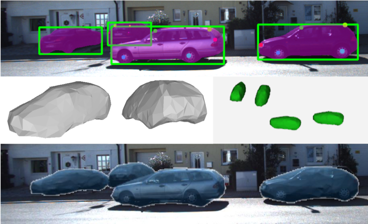
Figure 1: Our objective is to build detailed environment maps incorporating object poses and shapes. The figure from KITTI [20] in the top row shows the kind of information that our method relies on: bounding boxes (green), segmentation masks (magenta) and semantic keypoints (multiple colors). The middle row includes the reconstructed mesh models and 3D configuration. The last row shows the projection result.

II Related Work

The problem of incorporating semantic information in SLAM has gained increasing attention in recent years [4, 21]. In an early approach [22], objects are inserted in the map based on matching of feature descriptors to the models in a database, constructed offline using structure from motion. The camera trajectory provides multi-view information for object pose estimation but the object detections are not used as constraints to optimize the camera trajectory. Recent works often consider the optimization of object and camera poses simultaneously. SLAM++ [23] optimizes the camera and object poses jointly using a factor graph and moreover reconstructs dense surface mesh models of pre-defined object categories. A limitation of this work is that the estimated object shapes are pre-defined and rigid instead of being optimized to match the specific instances detected online.

The popularity of joint optimization of camera and object poses keeps increasing with the advent of robust 2-D object detectors based on structured models [24] and deep neural networks [25, 26]. The stacked hourglass model [13] is used by several works [14, 27] to extract mid-level object parts and, in turn, perform factor graph inference to recover the global positions and orientations of objects detected from a monocular camera. In [28], a deep network object detector is used to generate object hypotheses, which are subsequently validated using geometric and semantic cues and optimized via nonlinear filtering. Some of these approaches [29, 27, 28] use inertial measurements and probabilistic data association among detections and objects as additional constraints in the optimization. While most approaches focus on static objects, [30] uses a stereo camera to track ego-motion and dynamic 3-D objects in urban driving scenarios. The authors use bundle adjustment to fuse 3-D object measurements obtained from detection and viewpoint classification.

Various 3D object representations, including pointclouds [31, 32], voxels [33, 34], meshes [19, 35], and quadrics [36, 12], have been proposed in the literature. We are particularly interested in object models that can be constrained from multi-view observations and can adapt their pose and shape to specific object instances observed online. Tulsiani, Kar, et al. [32] learn a deformable pointcloud model with mean shape and deformation bases to fit object silhouettes at test time. The perspective transformer nets [33] use perspective projection to synthesize observations from different views and can be utilized for multi-view shape optimization. Introducing object models into the online inference process of SLAM requires compact representations that can be optimized and stored efficiently. QuadricSLAM [36, 12] parameterizes objects using dual ellipsoids, which can be extracted directly from bounding box detections and optimized using few parameters. A triangular mesh model of object shapes is proposed by [35] and is optimized from a single image using object keypoints and silhouettes. The optimization proceses uses approximate gradients of a mesh rasterization function obtained via the neural mesh renderer [19]. In this work, we generalize the deformable mesh model to $SE(3)$ camera and object poses and allow multi-view constraints and multi-object reconstruction.

III Problem Formulation

We consider the problem of detecting, localizing, and estimating the shape of object instances present in the scene, and estimating the pose of a camera over time. The states we are interested in estimating are the camera poses $\mathcal{C}\triangleq\{c_{t}\}_{t=1}^{T}$ with $c_{t}\in SE(3)$ and the object shapes and poses $\mathcal{O}\triangleq\{o_{n}\}_{n=1}^{N}$. More precisely, a camera pose $c_{t}:=(R_{c_{t}},p_{c_{t}})$ is determined by its position $p_{c_{t}}\in\mathbb{R}^{3}$ and orientation $R_{c_{t}}\in SO(3)$, while an object state $o_{n}=(\mu_{n},R_{o_{n}},p_{o_{n}})$ consists of a pose $R_{o_{n}}\in SO(3)$, $p_{o_{n}}\in\mathbb{R}^{3}$ and shape $\mu_{n}$, specified as a 3-D triangular mesh $\mu_{n}=(V_{n},F_{n})$ in the object canonical frame with vertices $V_{n}\in\mathbb{R}^{3\times|V_{n}|}$ and faces $F_{n}\in\mathbb{R}^{3\times|F_{n}|}$. Each row of $F_{n}$ contains the indices of 3 vertices that form a triangular face. A subset of the mesh vertices are designated as keypoints – distinguishing locations on an object’s surface (e.g., car door, windshield, or tires) that may be detected using a camera sensor. We define a keypoint association matrix $A_{n}\in\mathbb{R}^{|V_{n}|\times|K_{n}|}$ that generates $|K_{n}|$ keypoints $K_{n}=V_{n}A_{n}$ from all mesh vertices.

Suppose that a sequence $\mathcal{I}\triangleq\{i_{t}\}^{T}_{t=1}$ of $T$ images $i_{t}\in\mathbb{R}^{W\times H}$, collected from the corresponding camera poses $\{c_{t}\}_{t=1}^{T}$, are available for the estimation task. From each image $i_{t}$, we extract a set of object observations $\mathcal{Z}_{t}\triangleq\{z_{lt}=(\xi_{lt},s_{lt},y_{lt})\}_{l=1}^{L_{t}}$, consisting of a detected object’s category $\xi_{lt}\in\Xi$, a segmentation masks $s_{lt}\in\{0,1\}^{W\times H}$ and the pixel coordiantes of detected keypoints $y_{lt}\in\mathbb{R}^{2\times|K_{lt}|}$. We suppose that $\Xi$ is a finite set of pre-defined detectable object categories and that the data association $n=\pi_{t}(l)$ of observations to object instances is known (we describe an object tracking approach in Sec. IV-A but global data association can also be performed [37, 38, 29]). See Fig. 1 for example object observations.

For a given estimate of the camera pose $\hat{c}_{t}$ and the object state $\hat{o}_{n}$, we can predict expected semantic mask $\hat{s}_{lt}$ and semantic keypoint observations $\hat{y}_{lt}$ using a perspective projection model:

$$\hat{s}_{lt} =\mathcal{R}_{\text{mask}}(\hat{c}_{t},\hat{o}_{n})$$ (1)

$$\hat{y}_{lt} =\mathcal{R}_{\text{kps}}(\hat{c}_{t},\hat{o}_{n},A_{n})$$

where the mask and keypoint projection functions $\mathcal{R}_{\text{mask}}$, $\mathcal{R}_{\text{kps}}$ will be defined precisely in Sec. IV. The camera and object estimates can be optimized by reducing the error between the predicted $\hat{\mathcal{Z}}_{1:T}$ and the actual $\mathcal{Z}_{1:T}$ observations. We define loss functions $\mathcal{L}_{\text{mask}}$, measuring discrepancy between semantic masks, and $\mathcal{L}_{\text{kps}}$, measuring discrepancy among semantic keypoints, as follows:

$$\mathcal{L}_{\text{mask}}(s,\hat{s})= -\frac{\|s\odot\hat{s}\|_{1}}{\|s+\hat{s}-s\odot\hat{s}\|_{1}}$$ (2)

$$\mathcal{L}_{\text{kps}}(y,\hat{y})= \|y-\hat{y}\cdot vis(\hat{y})\|_{F}^{2}$$

where $\odot$ is an element-wise product and $vis(\hat{y}_{lt})\in\{0,1\}^{|K_{n}|\times|K_{lt}|}$ is a binary selection matrix that discards unobservable object keypoints.

Problem.

Given object observations $\mathcal{Z}_{1:T}$, determine the camera poses $\mathcal{C}$ and object states $\mathcal{O}$ that minimize the mask and keypoint losses:

$$\min_{\mathcal{C},\mathcal{O}}\sum_{t=1}^{T}\sum_{l=1}^{L_{t}} \left(w_{\text{mask}}\mathcal{L}_{\text{mask}}(s_{lt},\mathcal{R_{\text{mask}}}(c_{t},o_{\pi_{t}(l)}))\right.$$ (3)

$$+\left.w_{\text{kps}}\mathcal{L}_{\text{kps}}\left(y_{lt},\mathcal{R}_{\text{kps}}(c_{t},o_{\pi_{t}(l)},A_{\pi_{t}(l)})\right)\right)$$

where $w_{\text{mask}}$, $w_{\text{kps}}$ are scalar weight parameters specifying the relative importance of the mask and keypoint loss functions.

IV Technical Approach

We begin by describing how the object observations $\mathcal{Z}_{t}$ are obtained. Next, we provide a rigorous definition of the perspective projection models in (1), which, in turn, define the loss functions in (2) precisely. Finally, in order to perform the optimization in (3), we derive the gradients of $\mathcal{L}_{\text{mask}}$ and $\mathcal{L}_{\text{kps}}$ with respect to $c_{t}$ and $o_{t}$.

IV-A Semantic Perception

We extract both category-level (object category $\xi_{lt}$ and keypoints $y_{lt}$) and instance-level (segmentation masks $s_{lt}$) semantic information from the camera images. For each frame, we first use pre-trained model [39] to get object detection results represented with bounding boxes and instance segmentations inside the boxes. Each object is assigned to one of the class labels in $\Xi$. Then we extract semantic keypoints $y_{lt}$ within the bounding box of each detected object using the pre-trained stacked hourglass model of [17], which is widely used for human-joint/object-keypoint detector. The $l$-th detection result at time $t$ contains the object category $\xi_{lt}\in\Xi$, keypoints $y_{lt}\in\mathbb{R}^{2\times|K_{lt}|}$, mask $s_{lt}\in\{0,1\}^{W\times H}$, bounding box $\beta_{lt}\in\mathbb{R}^{4}$ (2-D location, width, and height) as shown in Fig. 1, object detection confidence $u_{lt}\in\mathbb{R}$ and keypoint detection confidences $q_{lt}\in\mathbb{R}^{|K_{lt}|}$.

We develop an object tracking approach in order to associate the semantic observations obtained over time with the object instance that generated them. We extend the KLT-based ORB-feature-tracking method of [40] to track semantic features $y_{lt}$ by accounting for their individual labels (e.g., car wheel, car door) and share object category $\xi_{lt}$. In detail, let $z_{lt}$ be a semantic observation from a newly detected object at time $t$. The objective is to determine if $z_{lt}$ matches any of the semantic observations $z_{m,t+1}\in\mathcal{Z}_{t+1}$ at time $t+1$ given that both have the same category label, i.e., $\xi_{lt}=\xi_{m,t+1}$. We apply the KLT optical flow algorithm [41] to estimate the locations $y_{l,t+1}$ of the semantic features $y_{lt}$ in the image plane at time $t+1$. We use the segmentation mask $s_{m,t+1}$ of the $m$-th semantic observation to determine if $y_{l,t+1}$ are inliers (i.e., if the segmentation mask $s_{m,t+1}$ is $1$ at image location $y_{l,t+1}$) with respect to observation $m$. Let $in(y_{l,t+1},s_{m,t+1})\in\{0,1\}^{|K_{lt}|}$ return a binary vector indicating whether each keypoint is an inlier or not. We repeat the process in reverse to determine if the backpropagated keypoints $y_{m,t}$ of observation $m$ are inliers with respect to observation $l$. Eventually, we compute a matching score based on the inliers and their detection confidences:

$$M_{lm}=\sum_{k=1}^{K_{lt}}in(y_{l,t+1}^{(k)},s_{m,t+1}^{(k)})\cdot in(y_{m,t}^{(k)},s_{l,t}^{(k)})\cdot q_{lt}^{(k)}$$ (4)

where $q_{lt}^{(k)}$ is the $k$-th element of $q_{lt}$. Finally, we match observation $l$ to the observation at time $t+1$ that maximizes the score, i.e., $m^{*}=\arg\max_{k}M_{lm}$. If the object bounding boxes $\beta_{lt}$ and $\beta_{m^{*},t+1}$ have compatible width and height, we declare that object $l$ has been successfully tracked to time $t+1$. Otherwise, we declare that object track $l$ has been lost.

IV-B Mesh Renderer as an Observation Model

Next, we develop the observation models $\mathcal{R}_{\text{mask}}$ and $\mathcal{R}_{\text{kps}}$ that specify how a semantic observations $z=(\xi,s,y)$ is generated by a camera with pose $(R_{c},p_{c})\in SE(3)$ observing an object of class $\xi\in\Xi$ with pose $(R_{o},p_{o})\in SE(3)$ and mesh shape $\mu=(V,F)$ with keypoint association matrix $A$. Let $K$ be the intrinsic matrix of the camera, defined as:

$$K=\begin{bmatrix}fs_{u}&fs_{n}&c_{u}\\ 0&fs_{v}&c_{v}\end{bmatrix}\in\mathbb{R}^{2\times 3},$$ (5)

where $f$ is the focal length in meters, $(s_{u},s_{v})$ is the pixels per meter resolution of the image array, $(c_{u},c_{v})$ is the image center in pixels and $s_{n}$ is a rectangular pixel scaling factor. Let $x:=VAe_{k}\in\mathbb{R}^{3}$ be the coordinates of the $k$-th object keypoint in the object frame, where $e_{k}$ is a standard basis vector. The projection of $x$ onto the image frame can be determined by first projecting it from the object frame to the camera frame using $(R_{o},p_{o})$ and $(R_{c},p_{c})$ and then the perspective projection $\pi:\mathbb{R}^{3}\rightarrow\mathbb{R}^{3}$, and the linear transformation $K$. In detail, this sequence of transformations leads to the pixel coordinates of $x$ as follows:

$$y^{(k)}=K\pi(R_{c}^{T}(R_{o}x+p_{o}-p_{c}))\in\mathbb{R}^{2}$$ (6)

where the standard perspective projection function is:

$$\pi(x)=\begin{bmatrix}x_{1}/x_{3}&x_{2}/x_{3}&x_{3}/x_{3}\end{bmatrix}^{T}$$ (7)

Applying the same transformation to all object keypoints $VA$ simultaneously leads to the keypoint projection model:

$$\mathcal{R}_{\text{cam}}(c,o,A) :=R_{c}^{T}(R_{o}VA+(p_{o}-p_{c})\mathbf{1}^{T})$$ (8)

$$\mathcal{R}_{\text{kps}}(c,o,A) :=K\pi\mathcal{R}_{\text{cam}}(c,o,A)$$

where $\mathbf{1}$ is a vector whose elements are all equal to $1$.

To define $\mathcal{R}_{\text{mask}}$, we need an extra rasterization step, which projects the object faces $F$ to the image frame. A rasterization function, $Raster(\cdot)$, can be defined using the standard method in [42], which assumes that if multiple faces are present, only the frontmost one is drawn at each pixel. Kato et al. [19] also show how to obtain an approximate gradient for the rasterization function. Relying on [42] and [19] for $Raster(\cdot)$, we can define the mask projection model:

$$\mathcal{R}_{\text{mask}}(c,o):=Raster\left(\mathcal{R}_{\text{cam}}(c,o,I),F\right)$$ (9)

Now that the projection models (1) and hence the loss functions (2) have been well defined, the final step needed to perform the optimization in (3) is to derive their gradients. We assume that the connectivity $F$ of the object mesh is fixed and the mesh is deformed only by changing the locations of the vertices $V$. We use the results of [19] for the gradient $\nabla_{V}Raster(V,F)$. Since $\mathcal{R}_{\text{mask}}$ is a function of $\mathcal{R}_{\text{cam}}$ according to (9), we only need to derive the following:

$$\nabla_{\hat{s}}\mathcal{L}_{\text{mask}}(s,\hat{s}),\; \nabla_{\hat{y}}\mathcal{L}_{\text{kps}}(y,\hat{y}),$$ (10)

$$\nabla_{c}\mathcal{R}_{\text{kps}}(c,o,A),\; \nabla_{o}\mathcal{R}_{\text{kps}}(c,o,A).$$

Our results are summarized in the following propositions.

Proposition 1.

The gradients of the loss functions $\mathcal{L}_{\text{mask}}(s,\hat{s})$ and $\mathcal{L}_{\text{kps}}(y,\hat{y})$ in (2) with respect to the estimated mask $\hat{s}\in\{0,1\}^{W\times H}$ and keypoint pixel coordinates $\hat{y}\in\mathbb{R}^{2\times K}$ are:

$$\nabla_{\hat{y}}\mathcal{L}_{\text{kps}}(y,\hat{y}) =2\,(\hat{y}\cdot vis(\hat{y})-y)\,vis(\hat{y})^{T}$$ (11)

$$\nabla_{\hat{s}}\mathcal{L}_{\text{mask}}(s,\hat{s}) =-\frac{1}{U(s,\hat{s})}\cdot s+\frac{I(s,\hat{s})}{U^{2}(s,\hat{s})}\cdot(\mathbf{1}\mathbf{1}^{T}-s)$$

where $I(s,\hat{s}):=\|s\odot\hat{s}\|_{1}$ and $U(s,\hat{s}):=\|s+\hat{s}-s\odot\hat{s}\|_{1}$.

Proposition 2.

Let $y^{(i)}=\mathcal{R}_{\text{kps}}(c,o,I)\in\mathbb{R}^{2}$ be the pixel coordinates of the $i$-th vertex $v_{i}:=Ve_{i}$ of an object with pose $(R_{o},p_{o})\in SE(3)$ obtained by projecting $v_{i}$ onto the image plane of a camera with pose $(R_{c},p_{c})\in SE(3)$, calibration matrix $K\in\mathbb{R}^{2\times 3}$. Let $\theta_{c},\theta_{o}\in\mathbb{R}^{3}$ be the axis-angle representations of $R_{c}$ and $R_{o}$, respectively, so that $R_{c}=\exp(\lfloor\theta_{c}\times\rfloor)$ and $R_{o}=\exp(\lfloor\theta_{o}\times\rfloor)$ and $\lfloor\cdot\times\rfloor$ is the hat map. Then, the derivative of $y^{(i)}$ with respect to $\alpha\in\{\theta_{c},p_{c},\theta_{o},p_{o},v_{i}\}$ is:

$$\frac{\partial y^{(i)}}{\partial\alpha}=K\frac{\partial\pi}{\partial x}(\gamma)\frac{\partial\gamma}{\partial\alpha}$$ (12)

where:

$$\frac{\partial\pi}{\partial x}(x) =\frac{1}{x_{3}}\begin{bmatrix}1&0&-x_{1}/x_{3}\\ 0&1&-x_{2}/x_{3}\\ 0&0&0\end{bmatrix}$$

$$\gamma =R_{c}^{T}(R_{o}v_{i}+p_{o}-p_{c})$$ (13)

$$\frac{\partial\gamma}{\partial p_{c}} =-R_{c}^{T}\quad\frac{\partial\gamma}{\partial p_{o}}=R_{c}^{T}\quad\frac{\partial\gamma}{\partial v_{i}}=R_{c}^{T}R_{o}$$

$$\frac{\partial\gamma}{\partial\theta_{c}} =R_{c}^{T}\lfloor(R_{o}v_{i}+p_{o}-p_{c})\times\rfloor J_{rSO(3)}(-\theta_{c})$$

$$\frac{\partial\gamma}{\partial\theta_{o}} =-R_{c}^{T}R_{o}\lfloor{v}_{i}\times\rfloor J_{rSO(3)}(\theta_{o})$$

and $J_{rSO(3)}(\theta)$ is the right Jacobian of $SO(3)$, which is necessary because the gradient needs to be projected from the tangent space to the $SO(3)$ manifold [43, Ch. 10.6], and can be computed in closed form:

$$J_{rSO(3)}(\theta)=I_{3}-\frac{1-\cos\|\theta\|}{\|\theta\|^{2}}\lfloor\theta\times\rfloor+\frac{\|\theta\|-\sin\|\theta\|}{\|\theta\|^{3}}\lfloor\theta\times\rfloor^{2}.$$ (14)

Proof.

By definition (8), $y^{(i)}=K\pi(\gamma)$ so most steps follow by the chain rule. We only discuss the relationship between the axis-angle vectors $\theta_{c}$, $\theta_{o}$ and the orientations $R_{c}$, $R_{o}$. Any rotation matrix $R\in SO(3)$ can be associated with a vector $\theta\in\mathbb{R}^{3}$ specifying it as a rotation about a fixed axis $\frac{\theta}{\|\theta\|_{2}}$ through an angle $\|\theta\|_{2}$. The axis-angle representation $\theta$ is related to $R$ through the exponential and logarithm maps:

$$\lfloor\theta\times\rfloor=\log(R)=\frac{\|\theta\|}{2\sin\|\theta\|}(R-R^{T})$$

See [44] and [43] for details. Consider the derivative of $\gamma$ with respect to $\theta_{o}$. The right Jacobian of $SO(3)$ satisfies the following for small $\delta\theta$:

$$\exp(\lfloor(\theta+\delta\theta)\times\rfloor)\approx\exp(\lfloor\theta\times\rfloor)\exp(\lfloor(J_{rSO(3)}(\theta)\delta\theta)\times\rfloor)$$

Using this and $R_{o}=\exp(\lfloor{\theta}_{o}\times\rfloor)$, we can compute:

$$\frac{\partial\gamma}{\partial\theta_{o}} =R_{c}^{T}\frac{\partial\exp(\lfloor\theta_{o}\times\rfloor)v_{i}}{\partial\theta_{o}}$$ (15)

$$=R_{c}^{T}R_{o}\frac{\partial}{\partial\delta\theta_{o}}\lfloor(J_{rSO(3)}(\theta_{o})\delta_{o}\theta)\times\rfloor v_{i}$$

$$=-R_{c}^{T}R_{o}\lfloor v\times\rfloor_{i}J_{rSO(3)}(\theta_{o})\frac{\partial\delta\theta_{o}}{\partial\delta\theta_{o}}$$

The derivative of $\gamma$ with respect to $\theta_{c}$ can be obtained using the same approach. ∎

In conclusion, we derived explicit definitions for the observation models $\mathcal{R}_{\text{kps}}$, $\mathcal{R}_{\text{mask}}$, the loss functions $\mathcal{L}_{\text{mask}}$, $\mathcal{L}_{\text{kps}}$, and their gradients directly taking the $SO(3)$ constraints into account via the axis-angle parameterization. As a result, we can treat (3) as an unconstrained optimization problem and solve it using gradient descent. The explicit gradient equations in Prop. 2 allow solving an object mapping-only problem by optimizing with respect to $\mathcal{O}$, a camera localization-only problem by optimizing with respect to $\mathcal{C}$, or a simultaneous localization and mapping problem.

IV-C Optimization Initialization

We implemented the localization and mapping tasks separately. In the localization task, we initialize the camera pose using inertial odometry obtained from integration of IMU measurements [1]. The camera pose is optimized sequentially between every two images via (3), leading to an object-level visual-inertial odometry algorithm.

To initialize the object model in the mapping task, we collect high-quality keypoints (according to $q_{lt}$ defined in Sec. IV-A) from multiple frames until an object track is lost. The 3-D positions of these keypoints are estimated by optimizing $\mathcal{L}_{\text{kps}}$ only using the Levenberg-Marquardt algorithm. Using a predefined category-level mesh model(mean model) with known keypoints, we apply the Kabsch algorithm [45] to initialize the object pose (i.e., the transformation from the detected 3-D keypoints to the category-level model keypoints). After initialization, we take two steps to optimize the object states. First, we fix the mesh vertices and optimize the pose based on the combined loss function in (3). Next, we fix the object pose, and optimize the mesh vertices using only the mask loss because the keypoint loss affects only few vertices. To improve the deformation optimization and obtain a smooth mesh model, we add regularization using the mean mesh curvature. The curvature is computed using a discretization of the continuous Laplace-Beltrami operator [46, 47]. Constraints from symmetric object categories can be enforced by directly defining the mesh shape model to be symmetric.

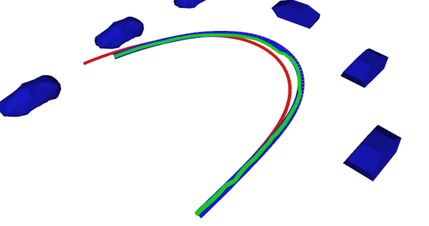
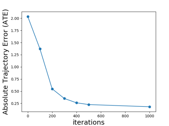
Figure 2: Left: Localization results from a simulated dataset, showing car poses (blue), the ground truth camera trajectory (blue), the inertial odometry used for initialization (red), and the optimized camera trajectory (green). Right: Change of Absolute Trajectory Error versus number of optimization iterations.

V Experiments

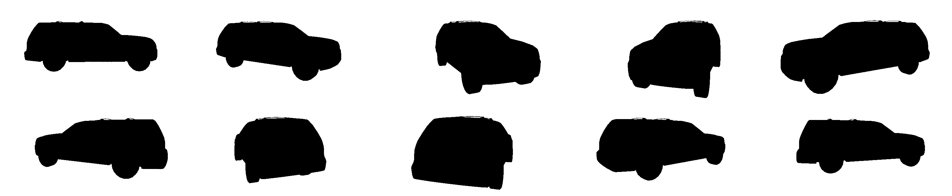
Figure 3: Views used to evaluate the object-level mapping approach in simulation.

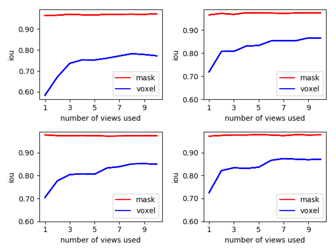
Figure 4: Mask and 3-D voxel intersection over union (IoU) results obtained with different numbers of object views for four different object instances (see Fig. 5).

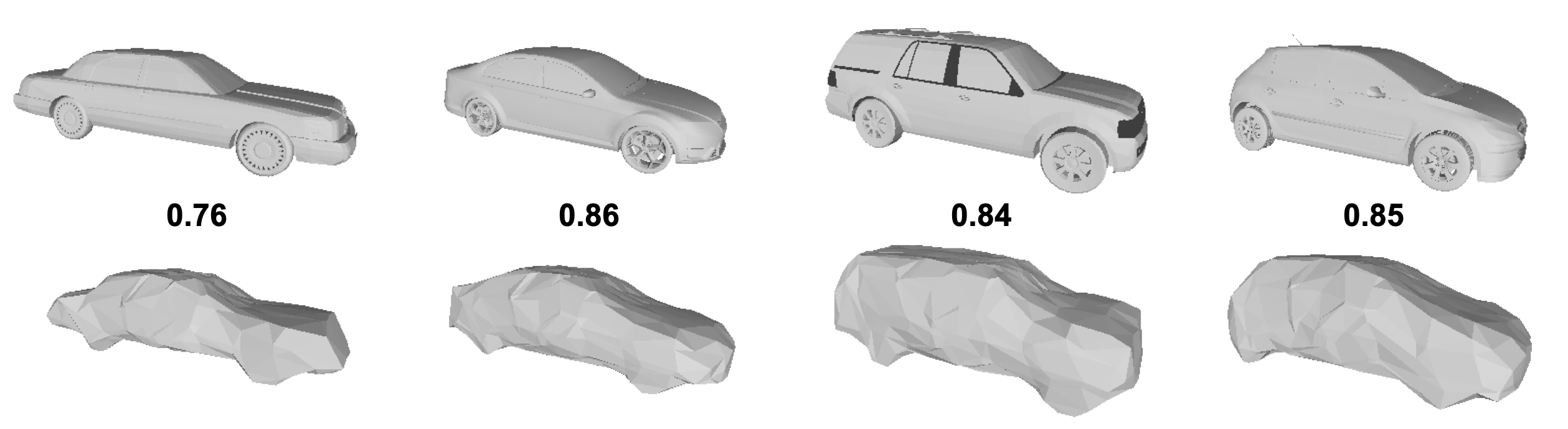
Figure 5: Qualitative comparison between estimated car shapes (bottom row) obtained from a simulation sequence and ground truth object meshes (top row). The numbers indicate 3D IoU.

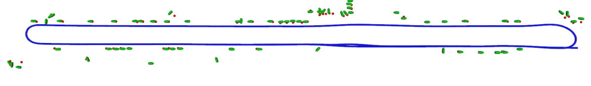
Figure 6: Qualitative results showing the accuracy of the estimated car positions (green) on sequence 06 of the KITTI odometry dataset in comparison with hand-labeled ground truth (red) obtained from [48]. The camera trajectory (blue) is shown as well.

Figure 7: Top: the semantic observations. Bottom: the projection of reconstructed mesh models.

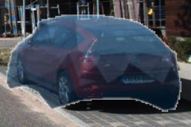
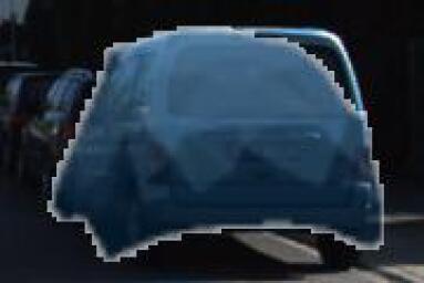
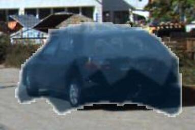
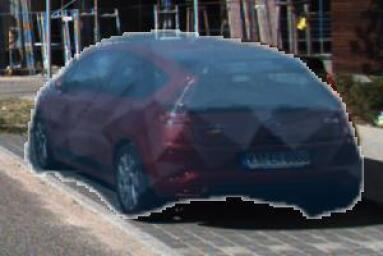
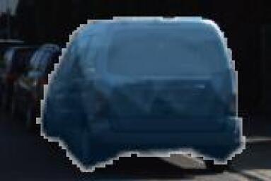
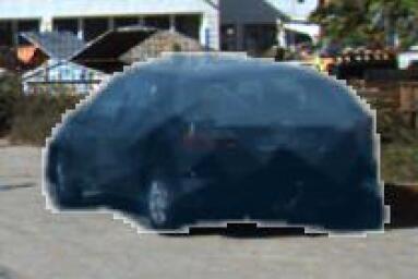
Figure 8: Top: category-level model before shape optimization. Bottom: instance-level model after shape optimization.

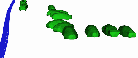
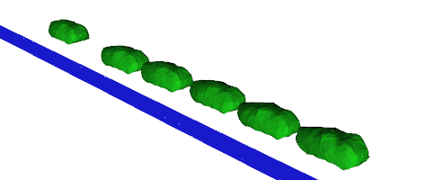
Figure 9: Left: 2D observation of mesh models. Right: corresponding 3D configuration. Trajectory in blue.

We evaluated the ability of the proposed localization and mapping technique to optimize the camera trajectory and reconstruct object poses and shapes using both simulated and real data. Our experiments used images from a monocular camera and inertial odometry information and focused on detecting, localizing and reconstructing cars object because 1) KITTI dataset with multiple cars is widely used and 2) there is pre-trained object detector and keypoint extractor for cars. We represented cars using a symmetric mesh model with 642 vertices and 1280 faces.

V-A Simulation Dataset

To model the real mechanism of IMU, we chose a sub-sequence IMU measurement and associated groundtruth pose from synchronized KITTI odometry dataset. We collected camera images following the groundtruth pose in a simulated Gazebo environment populated with car mesh models, so that we simulated a real camera-IMU sensor (see Fig. 2). The car models were annotated with keypoints and both the car surface and the keypoints were colored in contrasting colors to simplify the semantic segmentation and keypoint detection tasks. The simulated experiments used ground-truth data association among the observations. We evaluated both the localization and the mapping tasks.

For the localization task, we used a sequence with 70 frames and synchronized IMU measurements and 6 known cars were placed around. We initialized the estimation by predicting the transformation between two camera poses based on the IMU odometry. Then, we optimized the predicted camera pose by solving problem (3) and used the IMU to predict the next pose. An example camera trajectory and the associated localization results are shown in Fig. 2. We can see that our optimization successfully reduced the error accumulated from IMU integration.

The mapping performance was evaluated on a sequence of images obtained from different views of a single object (see Fig. 3). The optimization was initialized using a generic category-level car mesh and its vertices were optimized based on the detected keypoints and segmentation masks. The mapping quality is evaluated qualitatively using the Intersection over Union (IoU) ratio between the predicted and groundtruth car masks volumes. In detail, the mask IoU compares the area differences between predicted binary car masks, while the voxel IoU compares the voxelized volume of the predicted and groundtruth car models. Fig. 4 shows the dependence of the mapping accuracy on the number of different views used. The optimized car meshes are shown in Fig. 5. The differences among car models are clearly visible in the reconstructed meshes and their shapes are very close to the corresponding groundtruth shapes. Using only a few views, the optimization process is able to deform the mesh vertices to fit the segmentation masks but not necessarily align the estimated model with the real 3-D shape. As more observations become available, the 3D IoU increases, which makes sense since different views can provide information about additional instance-level characteristics. Based only on 3 views, the IoU reaches over 0.8, while the generic category-level mesh has an average IoU of 0.63 with respect to the different object instances.

TABLE I: 2D projection mIoU with respect to object segmentation on three KITTI sequence [20]

Dataset	09_26	09_26	09_30
	0048	0035	0020
Frames	22	131	1101
Detected objects	6	28	77
Single image mesh prediction [35]	0.692	0.642	0.641
With pose estimation	0.735	0.656	0.689
With pose and shape estimation	0.778	0.675	0.725

V-B KITTI Dataset

Experiments with real observations were carried out using the KITTI dataset [20]. We choose three sequences with different lengths. The experiments used the ground-truth camera poses and evaluated only the mapping task. The object detector, semantic segmentation [39] and the keypoint detector [17] algorithms used pre-trained weights. Semantic observations were collected as described in Sec. IV-A. The poses and shapes of the detected cars were initialized and optimized as described in Sec. IV-C. Fig. 6 shows a bird-eye view of the estimated car poses and compares the results with the ground truth car positions provided in [48]. The poses and shapes of 56 out of 62 marked cars were reconstructed, with an average position error across all cars of 1.9 meters. Fig. 7 shows some estimated 3-D car mesh models projected back onto the camera images. Fig. 8 compares the differences between the category-level and instance-specific models. Fig. 9 shows the estimated model shapes and poses in 3D. Since groundtruth object shapes are not available, we evaluate the quality of shape reconstruction based on the 2D IoU compared with the observed instance segmentation masks. We trained a single-image mesh predictor [35] on car data from the PASCAL3D+ dataset [18] and calculated its mean IoU for individual objects over multiple frames. Table I shows that our multi-view optimization method improves the IoU by leveraging semantic information from multiple images. The reconstruction quality on the real dataset is limited by the accuracy of the semantic information because the optimization objective is to align the predicted car shapes with the observed semantic masks and keypoints. The viewpoint changes on the real dataset are smaller, making the reconstruction task harder than in simulation. The pose estimation relies heavily on the keypoint detections, which in some cases are not robust enough. Nevertheless, our approach is able to generate accurate instance-specific mesh models in an environment containing occlusion and different lighting conditions.

VI Conclusion

This work demonstrates that object categories, shapes and poses can be recovered from visual semantic observations. The key innovation is the development of differentiable keypoint and segmentation mask projection models that allow object shape to be used for simultaneous semantic mapping and camera pose optimization. In contrast with existing techniques, our method generates accurate instance-level reconstructions of multiple objects, incorporating multi-view semantic information. Future work will extend the mesh reconstruction to multiple object categories and will focus on data association techniques for object re-identification and loop closure. Our ultimate goal is to develop an online SLAM algorithm that unifies semantic, geometric, and inertial measurements to allow rich environment understanding and contextual reasoning.

References

- [1] A. Mourikis and S. Roumeliotis, “A Multi-State Constraint Kalman Filter for Vision-aided Inertial Navigation,” University of Minnesota, Tech. Rep., 2006.
- [2] M. Bloesch, S. Omari, M. Hutter, and R. Siegwart, “Robust visual inertial odometry using a direct EKF-based approach,” in IEEE/RSJ IROS, 2015, pp. 298–304.
- [3] T. Qin, P. Li, and S. Shen, “Vins-mono: A robust and versatile monocular visual-inertial state estimator,” IEEE Transactions on Robotics, vol. 34, no. 4, pp. 1004–1020, 2018.
- [4] C. Cadena, L. Carlone, H. Carrillo, Y. Latif, D. Scaramuzza, J. Neira, I. Reid, and J. J. Leonard, “Past, present, and future of simultaneous localization and mapping: Toward the robust-perception age,” IEEE Transactions on Robotics, vol. 32, no. 6, pp. 1309–1332, 2016.
- [5] J. Engel, T. Schöps, and D. Cremers, “LSD-SLAM: Large-scale direct monocular SLAM,” in ECCV, 2014.
- [6] R. Mur-Artal and J. D. Tardós, “ORB-SLAM2: an open-source SLAM system for monocular, stereo and RGB-D cameras,” IEEE Transactions on Robotics, vol. 33, no. 5, pp. 1255–1262, 2017.
- [7] R. Newcombe, “Dense Visual SLAM,” Ph.D. dissertation, Imperial College London, 2012.
- [8] T. Whelan, R. Salas-Moreno, B., A. Davison, and S. Leutenegger, “ElasticFusion: Real-Time Dense SLAM and Light Source Estimation,” IJRR, vol. 35, no. 14, pp. 1697–1716, 2016.
- [9] D. G. Lowe, “Distinctive image features from scale-invariant keypoints,” International journal of computer vision, vol. 60, no. 2, pp. 91–110, 2004.
- [10] E. Rublee, V. Rabaud, K. Konolige, and G. Bradski, “ORB: An efficient alternative to SIFT or SURF,” in IEEE International Conference on Computer Vision (ICCV), 2011, pp. 2564–2571.
- [11] M. Kaess, “Simultaneous localization and mapping with infinite planes,” in IEEE Intl. Conf. on Robotics and Automation, ICRA, 2015.
- [12] M. Hosseinzadeh, Y. Latif, T. Pham, N. Sünderhauf, and I. D. Reid, “Towards semantic SLAM: points, planes and objects,” arXiv, vol. 1804.09111, 2018.
- [13] A. Newell, K. Yang, and J. Deng, “Stacked hourglass networks for human pose estimation,” in European Conference on Computer Vision. Springer, 2016, pp. 483–499.
- [14] G. Pavlakos, X. Zhou, A. Chan, K. G. Derpanis, and K. Daniilidis, “6-DoF Object Pose from Semantic Keypoints,” in IEEE International Conference on Robotics and Automation (ICRA), 2017.
- [15] Z. Yu, C. Feng, M. Liu, and S. Ramalingam, “CASENet: Deep Category-Aware Semantic Edge Detection,” in IEEE Conference on Computer Vision and Pattern Recognition (CVPR), 2017.
- [16] K. He, G. Gkioxari, P. Dollar, and R. Girshick, “Mask r-cnn.” IEEE transactions on pattern analysis and machine intelligence, 2018.
- [17] X. Zhou, A. Karpur, L. Luo, and Q. Huang, “Starmap for category-agnostic keypoint and viewpoint estimation,” in European Conference on Computer Vision (ECCV), 2018, pp. 318–334.
- [18] Y. Xiang, R. Mottaghi, and S. Savarese, “Beyond pascal: A benchmark for 3d object detection in the wild,” in IEEE Winter Conference on Applications of Computer Vision (WACV), 2014.
- [19] H. Kato, Y. Ushiku, and T. Harada, “Neural 3D Mesh Renderer,” in IEEE Conf. on Computer Vision and Pattern Recognition, 2018.
- [20] A. Geiger, P. Lenz, C. Stiller, and R. Urtasun, “Vision meets robotics: The KITTI dataset,” The International Journal of Robotics Research, vol. 32, no. 11, pp. 1231–1237, 2013.
- [21] A. J. Davison, “FutureMapping: The Computational Structure of Spatial AI Systems,” arXiv, vol. 1803.11288, 2018.
- [22] J. Civera, D. Gálvez-López, L. Riazuelo, J. D. Tardós, and J. Montiel, “Towards semantic SLAM using a monocular camera,” in IEEE/RSJ Int. Conf. on Intelligent Robots and Systems (IROS), 2011.
- [23] R. F. Salas-Moreno, R. A. Newcombe, H. Strasdat, P. H. Kelly, and A. J. Davison, “SLAM++: Simultaneous Localisation and Mapping at the Level of Objects,” in IEEE Conference on Computer Vision and Pattern Recognition (CVPR), 2013, pp. 1352–1359.
- [24] P. Felzenszwalb, R. Girshick, D. McAllester, and D. Ramanan, “Object Detection with Discriminatively Trained Part-Based Models,” IEEE Trans. on PAMI, vol. 32, no. 9, pp. 1627–1645, 2010.
- [25] R. Girshick, J. Donahue, T. Darrell, and J. Malik, “Rich feature hierarchies for accurate object detection and semantic segmentation,” in IEEE CVPR, 2014.
- [26] K. He, X. Zhang, S. Ren, and J. Sun, “Deep residual learning for image recognition,” in IEEE CVPR, 2016.
- [27] N. Atanasov, S. Bowman, K. Daniilidis, and G. Pappas, “A Unifying View of Geometry, Semantics, and Data Association in SLAM,” in International Joint Conference on Artificial Intelligence (IJCAI), 2018.
- [28] X. Fei and S. Soatto, “Visual-inertial object detection and mapping,” in European Conference on Computer Vision (ECCV), 2018.
- [29] S. Bowman, N. Atanasov, K. Daniilidis, and G. Pappas, “Probabilistic data association for semantic SLAM,” in IEEE International Conference on Robotics and Automation (ICRA), 2017, pp. 1722–1729.
- [30] P. Li, T. Qin, and S. Shen, “Stereo Vision-based Semantic 3D Object and Ego-motion Tracking for Autonomous Driving,” in European Conference on Computer Vision (ECCV), 2018, pp. 664–679.
- [31] H. Fan, H. Su, and L. Guibas, “A Point Set Generation Network for 3D Object Reconstruction from a Single Image,” in IEEE Conf. on Computer Vision and Pattern Recognition (CVPR), 2017.
- [32] S. Tulsiani, A. Kar, J. Carreira, and J. Malik, “Learning category-specific deformable 3d models for object reconstruction,” IEEE Trans. on PAMI, vol. 39, no. 4, pp. 719–731, 2017.
- [33] X. Yan, J. Yang, E. Yumer, Y. Guo, and H. Lee, “Perspective transformer nets: Learning single-view 3d object reconstruction without 3d supervision,” in Advances in Neural Information Processing Systems, 2016, pp. 1696–1704.
- [34] S. Tulsiani, T. Zhou, A. A. Efros, and J. Malik, “Multi-view supervision for single-view reconstruction via differentiable ray consistency,” in IEEE Conference on Computer Vision and Pattern Recognition (CVPR), 2017, pp. 209–217.
- [35] A. Kanazawa, S. Tulsiani, A. A. Efros, and J. Malik, “Learning category-specific mesh reconstruction from image collections,” in European Conference on Computer Vision (ECCV), 2018.
- [36] L. Nicholson, M. Milford, and N. Sünderhauf, “Quadricslam: Constrained dual quadrics from object detections as landmarks in semantic slam,” arXiv preprint arXiv:1804.04011, 2018.
- [37] J. Neira and J. D. Tardos, “Data association in stochastic mapping using the joint compatibility test,” IEEE Transactions on Robotics and Automation, vol. 17, no. 6, pp. 890–897, 2001.
- [38] M. Kaess and F. Dellaert, “Covariance recovery from a square root information matrix for data association,” Robotics and Autonomous Systems, vol. 57, no. 12, pp. 1198–1210, 2009.
- [39] F. Massa and R. Girshick, “maskrnn-benchmark: Fast, modular reference implementation of Instance Segmentation and Object Detection algorithms in PyTorch,” 2018.
- [40] K. Sun, K. Mohta, B. Pfrommer, M. Watterson, S. Liu, Y. Mulgaonkar, C. J. Taylor, and V. Kumar, “Robust stereo visual inertial odometry for fast autonomous flight,” IEEE Robotics and Automation Letters, vol. 3, no. 2, pp. 965–972, 2018.
- [41] B. D. Lucas and T. Kanade, “An Iterative Image Registration Technique with an Application to Stereo Vision,” in International Joint Conference on Artificial Intelligence (IJCAI), 1981.
- [42] S. Marschner and P. Shirley, Fundamentals of computer graphics. CRC Press, 2015.
- [43] G. Chirikjian, Stochastic Models, Information Theory, and Lie Groups, Volume 2: Analytic Methods and Modern Applications. Springer Science & Business Media, 2011, vol. 2.
- [44] Y. Ma, S. Soatto, J. Kosecka, and S. Sastry, An Invitation to 3-D Vision: from Images to Geometric Models. Springer Science & Business Media, 2012, vol. 26.
- [45] W. Kabsch, “A solution for the best rotation to relate two sets of vectors,” Acta Crystallographica, vol. 32, no. 5, pp. 922–923, 1976.
- [46] U. Pinkall and K. Polthier, “Computing discrete minimal surfaces and their conjugates,” Experimental mathematics, vol. 2, no. 1, 1993.
- [47] O. Sorkine, “Differential representations for mesh processing,” in Computer Graphics Forum, vol. 25, no. 4, 2006, pp. 789–807.
- [48] N. Atanasov, M. Zhu, K. Daniilidis, and G. J. Pappas, “Localization from semantic observations via the matrix permanent,” The International Journal of Robotics Research, vol. 35, no. 1-3, pp. 73–99, 2016.