Phase Reduction and Synchronization
of Coupled Noisy Oscillators

Abstract

We study the synchronization behavior of a noisy network in which each system is driven by two sources of state-dependent noise: (1) an intrinsic noise which is common among all systems and can be generated by the environment or any internal fluctuations, and (2) a coupling noise which is generated by interactions with other systems. After providing sufficient conditions that foster synchronization in networks of general noisy systems, we focus on weakly coupled networks of noisy oscillators and, using the first- and second-order phase response curves (PRCs), we derive a reduced order stochastic differential equation to describe the corresponding phase evolutions. Finally, we derive synchronization conditions based on the PRCs and illustrate the theoretical results on a couple of models.

Key words. Noisy networks, stochastic synchronization, phase reduction, first-order phase response curve, second-order phase response curve, stochastic averaging theory.

1 Introduction

Coupled oscillator models are fundamental in modeling and analyzing the synchronization behavior of systems with rhythmic behavior, including systems in ecology, neuroscience, and engineering [1, 2, 3, 4, 5, 6, 7]. These simple models often miss environmental fluctuations as well as internal and external disturbances. Therefore, a stochastic dynamics approach provides a significant compromise to keep modeling complexity tractable and still capture important phenomena.

Phase Response Curves (PRCs), which are computable both mathematically and experimentally [1, 8, 9, 10], provide fundamental information about how these oscillator models perform in a neighborhood of a stable limit cycle and facilitate a reduction of a high dimensional model to a 1-dimensional phase model. Furthermore, when multiple oscillator models interact with each other, such 1-dimensional reduced models enable the development of coupled oscillator models that use only the phase information and relative timing of their limit cycles.

PRC theory is typically developed for small deterministic perturbations around a stable limit cycle and in such cases it is sufficient to consider only the first order effects of the perturbation on the limit cycle. In this paper, we consider stochastic perturbations to the limit cycle and develop a stochastic phase reduced model.

The idea of phase reduction goes back at least to [11] and has been expanded and formalized in subsequent works, including [12, 1, 13]. The references [14, 15, 16] provide a good tutorial introduction to the topic. Phase reduction for noisy oscillators has also received remarkable attention [4, 3, 17, 18, 19, 20, 21, 22, 23, 24, 25, 26, 27]. Compared with these works, we provide complementary techniques that illuminate phase reduction from a PRCs perspective. Ermentrout et al. [28] and Teramae et al. [29, 17] consider a setup very similar to that studied in the present paper. However, their computations rely on the Stratonovich interpretation of stochastic differential equations, which leads to different reduced order models than those derived below using the Itô interpretation.

Our main goal is to find conditions that foster synchronization in networks of weakly coupled stochastically perturbed oscillators. In such networks, the oscillators can sense a common perturbation or perturbation through their interactions with other oscillators in the network. Toward this end, we contribute two types of results. First, we provide conditions that foster synchronization in a network of systems which sense two different sources of noise: (1) an intrinsic state-dependent noise which is common among all systems and can be generated by the environment or any internal fluctuations, and (2) a state-dependent coupling noise which is generated by interactions with other systems. Although our goal is to study a network of weakly coupled oscillators, our first result is not limited to such a network and is valid for more general networks. Second, we develop a stochastic phase reduced model for a network of weakly coupled noisy oscillators, where we use the notion of first- and second-order phase response curves, and averaging theory for stochastic differential equations. Finally, we apply the developed stochastic synchronization theory to the coupled phase equations to obtain the desired results.

The remainder of the paper is organized as follows. In Section 2, we prove the main results of this paper. After introducing noisy networks and defining stochastic synchronization, we provide conditions that foster stochastic synchronization in noisy networks. In Section 3, we recall some background on PRCs and phase reduction. In Section 4, we derive the phase reduced model for noisy oscillators and develop computational techniques to determine second-order PRCs. In Section 5, we derive the phase reduced model for weakly coupled noisy oscillators In Section 6, we apply the results of Section 2 to the phase reduced models in Section 5 to find conditions that foster synchronization in weakly coupled noisy oscillators. We illustrate these theoretical results on a couple of models. Finally, we conclude in Section 7.

2 Stochastic synchronization in noisy networks

In this section, we consider a noisy network of $N$ nonlinear systems with two sources of state-dependent noise: (1) an intrinsic noise which is common among all systems and can be generated by the environment or any internal fluctuations, and (2) a coupling noise which is generated by interactions with other systems. For $i=1,\ldots,N$, let the stochastic differential equation (SDE)

$$d\phi_{i}\;=\;\underbrace{\mathcal{F}(\phi_{i}{\color[rgb]{0,0,0}{,t}})dt+\sigma{\mathcal{K}}(\phi_{i}{\color[rgb]{0,0,0}{,t}})dW}_{\text{intrinsic dynamics}}\;+\underbrace{\displaystyle\sum_{j=1}^{N}c_{ij}\left(\epsilon\mathcal{H}({\color[rgb]{0,0,0}{\phi_{j},\phi_{i}}})dt+\delta\mathcal{C}({\color[rgb]{0,0,0}{\phi_{j},\phi_{i}}})dW_{ij}(t)\right)}_{\text{coupling dynamics}}$$ (1)

describe the dynamics of system $i$ with state $\phi_{i}\in\mathbb{R}^{n}$. The intrinsic and coupling dynamics of system $i$ are described as below.

Intrinsic dynamics. The systems are identical and governed by an $n-$dimensional vector of nonlinear functions, $\mathcal{F}$. There is a source of noise in (1) which is common among all the systems in the network and described by $\sigma\mathcal{K}(\phi_{i}{\color[rgb]{0,0,0}{,t}})dW$. The constant $\sigma\geq 0$ is the common noise intensity, $\mathcal{K}(\phi_{i}{\color[rgb]{0,0,0}{,t}})\in\mathbb{R}^{n\times n}$, and $W$ is an $n-$dimensional vector of independent standard Wiener processes.

Coupling dynamics. Denote the underlying network graph by $\mathcal{G}$ and assume that it is an undirected and weighted graph with weight $c_{ij}$, i.e., $c_{ij}=c_{ji}\geq 0$, with $c_{ij}>0$ if $i$ and $j$ are connected; and $c_{ij}=0$ if $i$ and $j$ are not connected. The interaction between system $i$ and another system, say $j$, influences the dynamics of $i$ through a deterministic term $c_{ij}\epsilon\mathcal{H}(\phi_{j},\phi_{i})dt$ and a stochastic term $c_{ij}\delta\mathcal{C}(\phi_{j},\phi_{i})dW_{ij}$, where $\mathcal{C}(\phi_{j},\phi_{i})\in\mathbb{R}^{n\times n}$, and $\mathbf{W}_{i}=(W_{i1},\ldots,W_{iN})^{\top}$ is a vector of independent standard Wiener processes. The constants $\epsilon\geq 0$ and $\delta\geq 0$ respectively describe the coupling strength and interaction noise intensity of the overall network while $\epsilon c_{ij}$ and $\delta c_{ij}$ respectively specify the coupling strength and noise intensity of each connection. We further assume that if $\epsilon=0$ or $\mathcal{H}\equiv 0$ then $\delta=0$.

For now, we only assume that $\mathcal{F}$, $\mathcal{H}$, $\mathcal{K}$, and $\mathcal{C}$ are nonlinear functions and they are nice enough so that (1) has a unique solution, for example, they are Lipschitz and satisfy a linear growth condition. See [30, Section 2.3] for more details. Later in Theorems 1 and 2 below, we will discuss appropriate conditions of these functions.

Equation (1) represents a broad range of network dynamics that can model many biological systems. For example, this framework covers the interconnected Kuramoto phase oscillators that model the brain’s neural activity where the neural dynamics are subject to noise. The level of a functional connection between two regions is proportional to synchronization between the oscillators’ phases associated with the two regions [31]. As another example, the framework covers a coupled bursting models [32, 33] that approximate the dynamics of coupled central pattern generators (CPGs) [34, 35] which are complex networks of neurons that produce rhythmic behaviors, such as walking. Synchronization properties and clusters formation of coupled CPGs explain the generation of various gait patterns in animal locomotions [36, 37].

After reviewing definitions of stochastic stability and stochastic synchronization, in Theorems 1-3, we will provide sufficient conditions that foster stochastic synchronization in (1).

Definition 1 (Stochastic stability).

Let $x(t)$ be a solution of an SDE. Then,

Moment exponential stability.

$x(t)$ is $p-$th ($p>0$) moment exponentially stable if there are a pair of positive constants $C$ and $c$ and a neighborhood $\Omega_{0}$ of $x(0)$ such that for any solution $y$ with $y(0)\in\Omega_{0}$

$$\mathbb{E}\|y(t)-x(t)\|^{p}<C\;\mathbb{E}\|y(0)-x(0)\|^{p}e^{-ct},\quad\forall t>0,$$

where $\mathbb{E}$ denotes the expected value and $\|\cdot\|$ denotes the Euclidean norm. When $p=2$, it is said to be exponentially stable in mean square.

Almost sure exponential stability.

$x(t)$ is almost sure exponentially stable if there is a neighborhood $\Omega_{0}$ of $x(0)$ such that for any solution $y$ with $y(0)\in\Omega_{0}$

$$\limsup_{t\to\infty}\dfrac{1}{t}\;\log\|y(t)-x(t)\|<0,\quad\text{almost surely (a.s.), }$$

which means $\mathbb{P}\left\{\limsup_{t\to\infty}\frac{1}{t}\;\log\|y(t)-x(t)\|<0\right\}=1$.

Definition 2 (Stochastic invariance).

A set $\mathcal{S}$ is called an invariance set for an SDE, if for any $x_{0}\in\mathcal{S}$,

$$\mathbb{P}\left\{x(t)\in\mathcal{S},\;\forall t\geq 0\right\}=1,$$

where $x(t)$ is a solution of the SDE starting from $x_{0}$ at $t=0$.

Moreover, for a fixed $p>0$, $\mathcal{S}$ is called $p-$th moment (respectively, almost sure) exponentially stable if any $x\in\mathcal{S}$ is $p-$th moment (respectively, almost sure) exponentially stable.

Definition 3 (Stochastic synchronization).

Let $\mathcal{S}$ be the set of states $x=(x_{1},\ldots,x_{N})^{\top}$ such that $x_{1}=\cdots=x_{N}$, i.e., $\mathcal{S}:=\{x\;|\;x_{1}=\cdots=x_{N}\}$. We say that $\mathcal{S}$ is a synchronization manifold if it is stochastically invariant and ($p-$th moment or almost surely) exponentially stable. We say that a network stochastically synchronizes if it admits a synchronization manifold, i.e., there exist $c,C>0$ such that for any solution $x(t)$, there exists $s(t)\in\mathcal{S}$ such that

$$\mathbb{E}\|x(t)-s(t)\|^{p}<C\;\mathbb{E}\|x(0)-s(0)\|^{p}e^{-ct},\quad\forall t>0,$$ (2)

or for any solution $x(t)$, there exists $s(t)\in\mathcal{S}$ such that

$$\limsup_{t\to\infty}\dfrac{1}{t}\;\log\|x(t)-s(t)\|<0,\quad a.s.$$

There have been some efforts to find conditions for synchronization in stochastic networks. For example, in [38] a sufficient condition for synchronization in a stochastic network of nonlinear systems is given. In this reference, the authors consider nonlinear state- (and time-) dependent diffusion matrices, however, they assume that the deterministic coupling is linear, i.e., $\mathcal{H}$ is assumed to be linear. In [39] the authors consider a stochastic network of nonlinear systems with linear coupling and a common noise. Here, we study the synchronization properties of a network of nonlinear systems in the presence of both nonlinear noisy coupling functions and nonlinear common noise. There are also some interesting results which guarantee synchronization onset in networks with no coupling but common noise, i.e., $\epsilon=\delta=0$ and $\sigma>0$, [29].

Although the systems in (1) can be of any arbitrary dimension, in the following theorem, for the ease of notation, we assume that the state variables are 1-dimensional, $n=1$.

We denote the Laplacian matrix of the underlying network graph $\mathcal{G}$ by $L_{[c]}$ (where the subscript $[c]$ represents the weights $c_{ij}$s) and its eigenvalues by $0=\lambda_{1,[c]}\leq\lambda_{2,[c]}\leq\cdots\leq\lambda_{N,[c]}$.

Theorem 1 (Stochastic synchronization: exponential stability in mean square).

Fix $\Omega_{1}\subset\mathbb{R}$ and let $\Omega_{2}:=\{x-y\;|\>x,y\in\Omega_{1}\}$. Consider (1) and assume that:

1. there exists a constant $\bar{c}_{\mathcal{F}}$ such that for all $x,y\in\Omega_{1}$ and $t\geq 0$,

   $$(x-y)(\mathcal{F}(x{\color[rgb]{0,0,0}{,t}})-\mathcal{F}(y{\color[rgb]{0,0,0}{,t}}))\leq\bar{c}_{\mathcal{F}}(x-y)^{2};$$

2. $\mathcal{H}:\Omega_{1}\times\Omega_{1}\to\mathbb{R}$ satisfies $\mathcal{H}(x,y)=-\mathcal{H}(y,x)$ and there exists a constant $\underline{c}_{\mathcal{H}}$ such that for all $x,y\in\Omega_{1}$, $\underline{c}_{\mathcal{H}}(x-y)^{2}\leq(x-y)\mathcal{H}(x,y)$;

3. there exists a non-negative constant $\bar{c}_{\mathcal{C}}$ such that for all $x,y\in\Omega_{1}$, $|\mathcal{C}(x,y)|\leq\bar{c}_{\mathcal{C}}|x-y|$; and

4. there exists a non-negative constant $\bar{c}_{\mathcal{K}}$ such that for all $x\in\Omega_{1}$ and $t\geq 0$,

   $$|\mathcal{K}(x{\color[rgb]{0,0,0}{,t}})-\mathcal{K}(y{\color[rgb]{0,0,0}{,t}})|\leq\bar{c}_{\mathcal{K}}|x-y|.$$

Then for any solution $(\phi_{1},\ldots,\phi_{N})^{\top}$,

$$\mathbb{E}\sum_{i=1}^{N}|\phi_{i}(t)-\psi(t)|^{2}<\mathbb{E}\sum_{i=1}^{N}|\phi_{i}(0)-\psi(0)|^{2}e^{-ct},\quad\forall t>0,$$

where $\psi(t)=\frac{1}{N}\sum_{i=1}^{N}\phi_{i}(t)$ and

$$c:=-2\bar{c}_{\mathcal{F}}+{2}\epsilon\underline{c}_{\mathcal{H}}\lambda-\delta^{2}\bar{c}_{\mathcal{C}}^{2}(1-\frac{1}{N})\lambda_{N,[c^{2}]}-\sigma^{2}\bar{c}_{\mathcal{K}}^{2}.$$ (3)

In (3), if $\underline{c}_{\mathcal{H}}>0$, then $\lambda=\lambda_{2,[c]}$, otherwise, $\lambda=\lambda_{N,[c]}$. $\lambda_{N,[c^{2}]}$ denotes the largest eigenvalue of the Laplacian matrix of network graph $\mathcal{G}$ with weights $c_{ij}^{2}$.

Therefore, the network stochastically synchronizes (in the sense of (2) with $p=2$) when $c>0$.

Proof.

The proof has three main steps:

Step 1. Introducing a synchronization manifold.

Let $(\phi_{1},\ldots,\phi_{N})^{\top}$ be a solution of (1), $\psi(t):=\frac{1}{N}\sum_{i=1}^{N}\phi_{i}(t)$ be the average of $\phi_{i}$’s, and $e_{i}:=\phi_{i}-\psi$ be the corresponding error. The dynamics of $(e_{1},\ldots,e_{N},\psi)$ can be written as:

$$\left(\begin{array}[]{c}de_{1}\\ \vdots\\ de_{N}\end{array}\right) =\left(\begin{array}[]{cccc}1-\frac{1}{N}&-\frac{1}{N}&\cdots&-\frac{1}{N}\\ &\ddots&&\\ -\frac{1}{N}&-\frac{1}{N}&\cdots&1-\frac{1}{N}\end{array}\right)_{N\times N}\left(\left(\begin{array}[]{c}\mathcal{F}(e_{1}+\psi{\color[rgb]{0,0,0}{,t}})\\ \vdots\\ \mathcal{F}(e_{N}+\psi{\color[rgb]{0,0,0}{,t}})\end{array}\right)+\epsilon\left(\begin{array}[]{c}{H_{1}}(e{\color[rgb]{0,0,0}{,\psi}})\\ \vdots\\ {H_{N}}(e{\color[rgb]{0,0,0}{,\psi}})\end{array}\right)\right)dt$$ (16)

$$+\left(\begin{array}[]{cccc}1-\frac{1}{N}&-\frac{1}{N}&\cdots&-\frac{1}{N}\\ &\ddots&&\\ -\frac{1}{N}&-\frac{1}{N}&\cdots&1-\frac{1}{N}\end{array}\right)_{N\times N}\left(\begin{array}[]{cccc}K(e,\psi{\color[rgb]{0,0,0}{,t}})\;|\;C_{1}(e{\color[rgb]{0,0,0}{,\psi}})\;|\;\cdots\;|\;C_{N}(e{\color[rgb]{0,0,0}{,\psi}})\end{array}\right)\left(\begin{array}[]{c}d{W}\\ d\mathbf{W}_{1}\\ \vdots\\ d\mathbf{W}_{N}\end{array}\right),$$ (25)

$$d\psi =\dfrac{1}{N}\sum_{i=1}^{N}\left(\mathcal{F}(e_{i}+\psi{\color[rgb]{0,0,0}{,t}})+\epsilon{H}_{i}(e{\color[rgb]{0,0,0}{,\psi}})\right)dt+\dfrac{\delta}{N}\sum_{i,j=1}^{N}c_{ji}\mathcal{C}(e_{j},e_{i})dW_{ij}+\dfrac{\sigma}{N}\sum_{i=1}^{N}\mathcal{K}(e_{i}+\psi{\color[rgb]{0,0,0}{,t}})dW,$$ (26)

where for $i=1,\ldots,N$,

$$H_{i}(e{\color[rgb]{0,0,0}{,\psi}}) =\epsilon\sum_{j=1}^{N}c_{ij}\mathcal{H}({\color[rgb]{0,0,0}{e_{j}+\psi,e_{i}+\psi}}),$$

$${K}(e,\psi{\color[rgb]{0,0,0}{,t}}) =\sigma(\mathcal{K}(e_{1}+\psi{\color[rgb]{0,0,0}{,t}})-\mathcal{K}(\psi{\color[rgb]{0,0,0}{,t}}),\ldots,\mathcal{K}(e_{N}+\psi{\color[rgb]{0,0,0}{,t}})-\mathcal{K}(\psi{\color[rgb]{0,0,0}{,t}}))^{\top},$$

and $C_{i}(e{\color[rgb]{0,0,0}{,\psi}})$ is an ${N\times N}$ matrix which its $i-$th row is $\delta(c_{i1}\mathcal{C}({\color[rgb]{0,0,0}{e_{1}+\psi,e_{i}+\psi}}),\ldots,c_{iN}\mathcal{C}({\color[rgb]{0,0,0}{e_{N}+\psi,e_{i}+\psi}})$ and its other rows are zero row vectors, and $d\mathbf{W}_{i}=(dW_{i1},\ldots,dW_{iN})^{\top}$ is an $N-$dimensional Wiener increment. We denote the $N\times N$ matrix in (16) by $A$.

Let $e=(e_{1},\ldots,e_{N})^{\top}$ and $\boldsymbol{y}=(e_{1},\ldots,e_{N},\psi)^{\top}$, and define $V({\color[rgb]{0,0,0}{\boldsymbol{y},t}})=\frac{1}{2}e^{\top}e$. Note that the set of zeros of $V$ is

$$\mathcal{S}:=\{(e_{1},\ldots,e_{N},\psi{\color[rgb]{0,0,0}{,t}})^{\top}\in\Omega_{2}^{N}\times\Omega_{1}{\color[rgb]{0,0,0}{\times[0,\infty)}}\;|\;e_{1}=\cdots=e_{N}=0\}.$$

This set is a candidate for the desired synchronization manifold. In the following two steps we show that if $c>0$, then $V$ becomes a Lyapunov function where $\dot{V}(\boldsymbol{y},t)\leq-c<0$. Then we conclude that $\mathcal{S}$ is an exponentially stable invariant set for (16)-(26) and therefore it is the synchronization manifold.

Step 2. Invariance of the synchronization manifold.

Note that the Itô derivative of $V$ is equal to

$$dV({\color[rgb]{0,0,0}{\boldsymbol{y},t}})=\mathcal{L}V({\color[rgb]{0,0,0}{\boldsymbol{y},t}})dt+V_{{\color[rgb]{0,0,0}{\boldsymbol{y}}}}{\color[rgb]{0,0,0}{(\boldsymbol{y},t)}}^{\top}g({\color[rgb]{0,0,0}{\boldsymbol{y},t}})dW,$$

where

$$\mathcal{L}V({\color[rgb]{0,0,0}{\boldsymbol{y},t}}):={\color[rgb]{0,0,0}{V_{t}(\boldsymbol{y},t)+}}V_{{\color[rgb]{0,0,0}{\boldsymbol{y}}}}({\color[rgb]{0,0,0}{\boldsymbol{y},t}})^{\top}f({\color[rgb]{0,0,0}{\boldsymbol{y},t}})+\frac{1}{2}\mathrm{tr}\left[g^{\top}({\color[rgb]{0,0,0}{\boldsymbol{y},t}})V_{\boldsymbol{y}\boldsymbol{y}}({\color[rgb]{0,0,0}{\boldsymbol{y},t}})g({\color[rgb]{0,0,0}{\boldsymbol{y},t}})\right].$$ (27)

The $(N+1)-$dimensional vectors $f({\color[rgb]{0,0,0}{\boldsymbol{y},t}})$ and $g({\color[rgb]{0,0,0}{\boldsymbol{y},t}})$ are respectively the drift and diffusion terms of (16)-(26), $V_{t}=\frac{\partial V}{\partial t}=0$, $V_{\boldsymbol{y}}=\frac{\partial V}{\partial\boldsymbol{y}}=(e^{\top},0)^{\top}$, and $V_{\boldsymbol{y}\boldsymbol{y}}(\boldsymbol{y},t)$ is the $(N+1\times N+1)$ Hessian matrix of $V$ which is a diagonal matrix with all entries equal to 1 except the last diagonal entry which is equal to 0. The trace operator is denoted by $\mathrm{tr}[\cdot]$. We show that there exists $c_{\mathcal{L}}>0$ such that $\mathcal{L}V\leq-c_{\mathcal{L}}V$. Then by [40, Theorem 1] we conclude that $\mathcal{S}$ is an invariant set for (16)-(26).

• Because $e_{1}+\cdots+e_{N}=0$, $e^{\top}A=e^{\top}$, and $e^{\top}\left(\begin{array}[]{c}\mathcal{F}(\psi{\color[rgb]{0,0,0}{,t}})\\ \vdots\\ \mathcal{F}(\psi{\color[rgb]{0,0,0}{,t}})\end{array}\right)=0$. Therefore, the second term of the right hand side of (27) becomes:

  $$V_{\boldsymbol{y}}(\boldsymbol{y},t)^{\top}f({\color[rgb]{0,0,0}{\boldsymbol{y},t}}) =(e^{\top},0)^{\top}f(e,\psi{\color[rgb]{0,0,0}{,t}})$$

  $$=(e_{1},\ldots,e_{N})\left\{\left(\begin{array}[]{c}\mathcal{F}(e_{1}+\psi{\color[rgb]{0,0,0}{,t}})\\ \vdots\\ \mathcal{F}(e_{N}+\psi{\color[rgb]{0,0,0}{,t}})\end{array}\right)+\left(\begin{array}[]{c}\mathcal{F}(\psi{\color[rgb]{0,0,0}{,t}})\\ \vdots\\ \mathcal{F}(\psi{\color[rgb]{0,0,0}{,t}})\end{array}\right)+\epsilon\left(\begin{array}[]{c}{H_{1}}(e{\color[rgb]{0,0,0}{,\psi}})\\ \vdots\\ {H_{N}}(e{\color[rgb]{0,0,0}{,\psi}})\end{array}\right)\right\}$$

  $$=\sum_{i=1}^{N}e_{i}(\mathcal{F}(e_{i}+\psi{\color[rgb]{0,0,0}{,t}})-\mathcal{F}(\psi{\color[rgb]{0,0,0}{,t}}))+\epsilon\sum_{i=1}^{N}e_{i}H_{i}(e{\color[rgb]{0,0,0}{,\psi}})$$

  By condition (i) and the definition of $V$, the first sum satisfies

  $$\sum_{i=1}^{N}e_{i}(\mathcal{F}(e_{i}+\psi{\color[rgb]{0,0,0}{,t}})-\mathcal{F}(\psi{\color[rgb]{0,0,0}{,t}})) \leq\bar{c}_{\mathcal{F}}\sum_{i=1}^{N}e_{i}^{2}=2\bar{c}_{\mathcal{F}}V(\boldsymbol{y},t).$$

  By condition (ii) and using $c_{ij}=c_{ji}$, the second sum satisfies

  $$\epsilon\sum_{i=1}^{N}e_{i}H_{i}(e{\color[rgb]{0,0,0}{,\psi}}) =\epsilon\sum_{i=1}^{N}e_{i}\sum_{j=1}^{N}c_{ji}\mathcal{H}({\color[rgb]{0,0,0}{e_{j}+\psi,e_{i}+\psi}})$$

  $$=\frac{\epsilon}{2}\sum_{i=1}^{N}\sum_{j=1}^{N}c_{ji}(e_{i}\mathcal{H}({\color[rgb]{0,0,0}{e_{j}+\psi,e_{i}+\psi}})+e_{j}\mathcal{H}({\color[rgb]{0,0,0}{e_{i}+\psi,e_{j}+\psi}}))$$

  $$=-\frac{\epsilon}{2}\sum_{i=1}^{N}\sum_{j=1}^{N}c_{ji}(e_{i}-e_{j})\mathcal{H}({\color[rgb]{0,0,0}{e_{i}+\psi,e_{j}+\psi}})$$ condition (ii)

  $$<-\frac{\epsilon}{2}\sum_{i=1}^{N}\sum_{j=1}^{N}c_{ji}\underline{c}_{\mathcal{H}}(e_{i}-e_{j})^{2}$$ condition (ii)

  $$=-{\epsilon}\underline{c}_{\mathcal{H}}e^{\top}L_{[c]}e,$$

  Since $e^{\top}v_{1}=0$, where $v_{1}=(1,\ldots,1)^{\top}$ is the eigenvector of $L_{[c]}$ corresponding to $\lambda_{1,[c]}=0$, by min-max theorem, $\lambda_{2,[c]}e^{\top}e\leq e^{\top}L_{[c]}e\leq\lambda_{N,[c]}e^{\top}e$. Therefore, depending on the sign of $\underline{c}_{\mathcal{H}}$, we have:

  $${\epsilon}\sum_{i=1}^{N}e_{i}H_{i}(e{\color[rgb]{0,0,0}{,\psi}}) <-{\epsilon}\underline{c}_{\mathcal{H}}e^{\top}L_{[c]}e\leq-{\epsilon}\underline{c}_{\mathcal{H}}\lambda_{2,[c]}e^{\top}e=-{2}\epsilon\underline{c}_{\mathcal{H}}\lambda_{2,[c]}V({\color[rgb]{0,0,0}{\boldsymbol{y},t}}) \underline{c}_{\mathcal{H}}>0$$ for , or

  $${\epsilon}\sum_{i=1}^{N}e_{i}H_{i}(e{\color[rgb]{0,0,0}{,\psi}}) <-{\epsilon}\underline{c}_{\mathcal{H}}e^{\top}L_{[c]}e\leq-{\epsilon}\underline{c}_{\mathcal{H}}\lambda_{N,[c]}e^{\top}e=-{2}\epsilon\underline{c}_{\mathcal{H}}\lambda_{N,[c]}V({\color[rgb]{0,0,0}{\boldsymbol{y},t}}) \text{for $\underline{c}_{\mathcal{H}}<0$}.$$

  Therefore, $V_{\boldsymbol{y}}(\boldsymbol{y},t)^{\top}f({\color[rgb]{0,0,0}{\boldsymbol{y},t}})\leq(2\bar{c}_{\mathcal{F}}-{2}\epsilon\underline{c}_{\mathcal{H}}\lambda)V(\boldsymbol{y},t).$

• A straightforward matrix multiplication implies that the third term of $\mathcal{L}V$ satisfies:

  $$\frac{1}{2}\mathrm{tr}\left[g^{\top}({\color[rgb]{0,0,0}{\boldsymbol{y},t}})V_{\boldsymbol{y}\boldsymbol{y}}(\boldsymbol{y},t)g({\color[rgb]{0,0,0}{\boldsymbol{y},t}})\right]=\frac{\delta^{2}}{2}\left(1-\frac{1}{N}\right)\sum_{i=1}^{N}\sum_{j=1}^{N}c_{ij}^{2}\mathcal{C}^{2}({\color[rgb]{0,0,0}{e_{j}+\psi,e_{i},\psi}})+{\frac{1}{2}\|A{K}(e,\psi{\color[rgb]{0,0,0}{,t}})\|^{2}},$$

  where by condition (iii)

  $$\frac{\delta^{2}}{2}\left(1-\frac{1}{N}\right)\sum_{i=1}^{N}\sum_{j=1}^{N}c_{ij}^{2}\mathcal{C}^{2}({\color[rgb]{0,0,0}{e_{j}+\psi,e_{i},\psi}}) \leq\frac{\delta^{2}}{2}\left(1-\frac{1}{N}\right)\bar{c}^{2}_{\mathcal{C}}\sum_{i=1}^{N}\sum_{j=1}^{N}c_{ij}^{2}(e_{j}-e_{i})^{2}$$

  $$=\frac{\delta^{2}}{2}\left(1-\frac{1}{N}\right)\bar{c}^{2}_{\mathcal{C}}e^{\top}L_{[c^{2}]}e$$

  $$\leq\frac{\delta^{2}}{2}\left(1-\frac{1}{N}\right)\bar{c}^{2}_{\mathcal{C}}\lambda_{N,[c^{2}]}e^{\top}e$$

  $$=\delta^{2}\left(1-\frac{1}{N}\right)\bar{c}^{2}_{\mathcal{C}}\lambda_{N,[c^{2}]}V(\boldsymbol{y},t).$$

  Using the fact that the largest eigenvalue of $A$ is equal to one and by condition (iv)

  $${\frac{1}{2}\|A{K}(e,\psi{\color[rgb]{0,0,0}{,t}})\|^{2}\leq\frac{1}{2}\|{K}(e,\psi{\color[rgb]{0,0,0}{,t}})\|^{2}=}\frac{\sigma^{2}}{2}\sum_{i=1}^{N}(\mathcal{K}(e_{i}+\psi{\color[rgb]{0,0,0}{,t}})-\mathcal{K}(\psi{\color[rgb]{0,0,0}{,t}}))^{2}\;\leq\;\frac{\sigma^{2}}{2}\sum_{i=1}^{N}\bar{c}_{\mathcal{K}}^{2}e_{i}^{2}\;=\;\sigma^{2}\bar{c}_{\mathcal{K}}^{2}V(\boldsymbol{y},t).$$

Therefor, $\mathcal{L}V(\boldsymbol{y},t)\leq-c_{\mathcal{L}}V(\boldsymbol{y},t)$ where $c_{\mathcal{L}}=c=-2\bar{c}_{\mathcal{F}}+{2}\epsilon\underline{c}_{\mathcal{H}}\lambda-\delta^{2}\bar{c}_{\mathcal{C}}^{2}(1-\frac{1}{N})\lambda_{N,[c^{2}]}-\sigma^{2}\bar{c}_{\mathcal{K}}^{2}.$ If $c>0$ then $\mathcal{L}V\leq-cV<0,$ and by [40, Theorem 1], $\mathcal{S}$ becomes an invariant set for (16)-(26).

Step 3. Stability of the synchronization manifold.

As we discussed in Step 2, the Itô derivative of $V$ is $dV(\boldsymbol{y},t)=\mathcal{L}(V(\boldsymbol{y},t))dt+V_{\boldsymbol{y}}^{\top}g(\boldsymbol{y},t)dW$. By Dynkin’s formula, $\mathbb{E}\int_{s}^{t}V_{\boldsymbol{y}}(\boldsymbol{y}(\tau),\tau)^{\top}g(\boldsymbol{y}(\tau),\tau)dW(\tau)=0$, and

$$\mathbb{E}V(\boldsymbol{y}(t),t)-\mathbb{E}V(\boldsymbol{y}(s),s) =\mathbb{E}\int_{s}^{t}dV(\boldsymbol{y}(\tau),\tau)\;d\tau$$

$$=\mathbb{E}\int_{s}^{t}\mathcal{L}V(\boldsymbol{y}(\tau),\tau)\;d\tau+\mathbb{E}\int_{s}^{t}V_{\boldsymbol{y}}(\boldsymbol{y}(\tau),\tau)^{\top}g(\boldsymbol{y}(\tau),\tau)dW(\tau)$$

$$=\mathbb{E}\int_{s}^{t}\mathcal{L}V(\boldsymbol{y}(\tau),\tau)\;d\tau$$ Dynkin’s formula,

$$\leq-c\;\mathbb{E}\int_{s}^{t}V(\boldsymbol{y}(\tau),\tau)\;d\tau$$ Step 2,

$$\leq-c\;\int_{s}^{t}\mathbb{E}V(\boldsymbol{y}(\tau),\tau)\;d\tau \text{Fubini's Theorem}.$$

The last inequality holds because $\mathbb{E}V(\boldsymbol{y}(\tau),\tau)$ is a continuous function of $\tau$ and hence its integral on $[s,t]$ is finite. Let $h(t)=\mathbb{E}V(\boldsymbol{y}(t),t)$, then by Gronwall’s Inequality, $h(t)-h(s)\leq-c\int_{s}^{t}h(\tau)\;d\tau$ implies that $h(t)\leq h(0)e^{-ct}$. Hence,

$$\mathbb{E}V(\boldsymbol{y}(t),t)\leq\mathbb{E}V(\boldsymbol{y}(0),0)e^{-ct}\quad\Rightarrow\quad\mathbb{E}\|e(t)\|^{2}\leq\mathbb{E}\|e(0)\|^{2}\;e^{-ct},$$

or equivalently,

$$\qquad\mathbb{E}\sum_{i=1}^{N}|\phi_{i}(t)-\psi(t)|^{2}\leq\mathbb{E}\sum_{i=1}^{N}|\phi_{i}(0)-\psi(0)|^{2}\;e^{-ct}.$$

If $c>0$, then $\mathcal{S}$ becomes exponentially stable. Therefore, by the definition of stochastic synchronization and Step 2, $\mathcal{S}$ becomes a synchronization manifold.

∎

In Theorem 1, we showed that if a network synchronizes in the absence of any noises (common noise or noise induced by the interactions among the nodes in the network), it could also synchronize in the presence of a sufficiently small noise and we found an upper bound for the noise intensities which guarantee such a behavior, i.e., we proved that if the noise intensities are such that $c>0$, then the network preserves its synchronization behavior. Unlike in Theorem 1, in the following theorem, $c$ can be negative and the system synchronizes. Indeed, the next result shows that noise intensities can be beneficial for networks synchronization.

Theorem 2 (Stochastic synchronization: $p-$th moment exponential stability).

Consider conditions (i-iv) of Theorem 1 and furthermore assume that

1. $\mathcal{C}:\Omega_{1}\times\Omega_{1}\to\mathbb{R}$ satisfies $\mathcal{C}(x,y)=-\mathcal{C}(y,x)$ (or $\mathcal{C}(x,y)=\mathcal{C}(y,x)$) and there exists a constant $\underline{c}_{\mathcal{C}}$ such that for all $x,y\in\Omega_{1}$, $\underline{c}_{\mathcal{C}}|x-y|\leq|\mathcal{C}(x,y)|$; and

2. there exists a non-negative constant $\underline{c}_{\mathcal{K}}$ such that for all $x,y\in\Omega_{1}$ and $t\geq 0$,

   $$\underline{c}_{\mathcal{K}}(x-y)^{2}\leq(x-y)(\mathcal{K}(x{\color[rgb]{0,0,0}{,t}})-\mathcal{K}(y{\color[rgb]{0,0,0}{,t}})).$$

Let

$$\alpha_{1}=-c/2,\quad\alpha_{2}^{2}=(\sigma\underline{c}_{\mathcal{K}})^{2}+\frac{\delta^{2}\underline{c}_{\mathcal{C}}^{2}\lambda_{2,[c]}^{2}}{12},$$

and assume that $0\leq\alpha_{1}<\alpha_{2}^{2}$. Then for $0<p<2(1-\frac{\alpha_{1}}{\alpha_{2}^{2}})\leq 2$ and $\alpha:=-p[(\frac{p}{2}-1)\alpha_{2}^{2}-\alpha_{1}]$ (which is positive), (1) stochastically synchronizes, i.e.,

$$\mathbb{E}\left(\sum_{i=1}^{N}|\phi_{i}(t)-\psi(t)|^{2}\right)^{p/2}\leq\mathbb{E}\left(\sum_{i=1}^{N}|\phi_{i}(0)-\psi(0)|^{2}\right)^{p/2}\;e^{-\alpha t}.$$

To prove Theorem 2, we use the following lemma which is a modified version of [30, Chapter 4, Corollary 4.6].

Lemma 1.

Consider $dx=f(x{\color[rgb]{0,0,0}{,t}})dt+g(x{\color[rgb]{0,0,0}{,t}})dW$ and assume that there exist constants $\alpha_{1}$ and $\alpha_{2}$ such that for any $t\geq 0$,

$$x^{\top}f(x{\color[rgb]{0,0,0}{,t}})+\frac{1}{2}\mathrm{tr}[g^{\top}(x{\color[rgb]{0,0,0}{,t}})g(x{\color[rgb]{0,0,0}{,t}})]\;\leq\;\alpha_{1}x^{\top}x,\quad\text{and}$$ (28)

$$\alpha_{2}x^{\top}x\leq\|x^{\top}g{\color[rgb]{0,0,0}{(x,t)}}\|.$$ (29)

If $0\leq\alpha_{1}<\alpha_{2}^{2}$, then the trivial solution of $dx=f(x{\color[rgb]{0,0,0}{,t}})dt+g(x{\color[rgb]{0,0,0}{,t}})dW$ is $p-$th moment exponentially stable provided $0<p<2(1-\frac{\alpha_{1}}{\alpha_{2}^{2}})\leq 2$ and $\alpha:=-p[(\frac{p}{2}-1)\alpha_{2}^{2}-\alpha_{1}]>0$, i.e., $\forall t>0$

$$\mathbb{E}\|x(t)\|^{p}<\mathbb{E}\|x(0)\|^{p}e^{-\alpha t}.$$

Proof of Theorem 2. Under the conditions of Theorems 1 and 2, we apply Lemma 1 to (16). The left hand side of (28) is equivalent to $\mathcal{L}(V(\boldsymbol{y},t))$ which we showed $\mathcal{L}(V(\boldsymbol{y},t))\leq-cV(\boldsymbol{y},t)=-\frac{c}{2}e^{\top}e$. Therefore, $\alpha_{1}=-c/2$. A straightforward matrix multiplications gives:

$$\|e^{\top}g\|^{2} =\|e^{\top}A\left(\begin{array}[]{cccc}K(e,\psi,t)\;|\;C_{1}(e,\psi)\;|\;\cdots\;|\;C_{N}(e,\psi)\end{array}\right)\|^{2}$$

$$=\|e^{\top}\left(\begin{array}[]{cccc}K(e,\psi,t)\;|\;C_{1}(e,\psi)\;|\;\cdots\;|\;C_{N}(e,\psi)\end{array}\right)\|^{2} e^{\top}A=e^{\top}$$

$$=\sigma^{2}\left(\sum_{i=1}^{N}e_{i}\mathcal{K}(e_{i}+\psi,t)\right)^{2}+\delta^{2}\sum_{i=1}^{N}e_{i}^{2}\sum_{j=1}^{N}c_{ij}^{2}\mathcal{C}^{2}(e_{j}+\psi,e_{i}+\psi)$$

$$=\sigma^{2}\left(\sum_{i=1}^{N}(e_{i}+\psi-\psi)(\mathcal{K}(e_{i}+\psi,t)-\mathcal{K}(\psi,t))\right)^{2} \mathcal{K}(\psi)\sum e_{i}=0$$

$$\quad+\frac{\delta^{2}}{2}\sum_{i,j=1}^{N}c_{ij}^{2}(e_{i}^{2}+e_{j}^{2})\mathcal{C}^{2}(e_{i}+\psi,e_{j}+\psi) \mathcal{C}(x,y)=\pm\mathcal{C}(y,x)$$

$$\geq(\sigma\underline{c}_{\mathcal{K}})^{2}\left(\sum_{i=1}^{N}e_{i}^{2}\right)^{2}$$ conditions (ii) & (i) of Theorem 2

$$\quad+\frac{\delta^{2}}{2}\frac{\underline{c}_{\mathcal{C}}^{2}}{2}\sum_{i,j=1}^{N}c_{ij}^{2}(e_{i}-e_{j})^{4} e_{i}^{2}+e_{j}^{2}\geq\frac{(e_{i}-e_{j})^{2}}{2}$$ and

$$\geq\left((\sigma\underline{c}_{\mathcal{K}})^{2}+\frac{\delta^{2}}{2}\frac{\underline{c}_{\mathcal{C}}^{2}}{2}\frac{\lambda_{2,[c]}^{2}}{{N}}\right)(e^{\top}e)^{2}.$$

The last inequality holds because $\sum c_{ij}^{2}(e_{i}-e_{j})^{4}=\sum(c_{ij}(e_{i}-e_{j})^{2})^{2}\geq\frac{1}{{N}}\left(\sum c_{ij}(e_{i}-e_{j})^{2}\right)^{2}.$ Therefore, $\alpha_{2}^{2}=(\sigma\underline{c}_{\mathcal{K}})^{2}+\dfrac{\delta^{2}\underline{c}_{\mathcal{C}}^{2}\lambda_{2,[c]}^{2}}{{4N}}$. By Lemma 1, for $p<2-2{\alpha_{1}}/{\alpha_{2}^{2}}$,

$$\mathbb{E}\left(\sum_{i=1}^{N}|\phi_{i}(t)-\psi(t)|^{2}\right)^{p/2}\leq\mathbb{E}\left(\sum_{i=1}^{N}|\phi_{i}(0)-\psi(0)|^{2}\right)^{p/2}\;e^{-\alpha t},$$

where $\alpha=p\alpha_{1}-p(p/2-1)\alpha_{2}^{2}$. ∎

Theorem 3 (Stochastic synchronization: almost sure exponential stability).

Consider conditions (i-iv) of Theorem 1 and conditions (i-ii) of Theorem 2. Then

$$\limsup_{t\to\infty}\dfrac{1}{t}\;\log(\|e(t)\|)\leq\alpha_{1}-\alpha_{2}^{2},\quad a.s.$$

Proof.

Proof by [30, Chapter 4, Theorem 4.3]. ∎

Remark 1.

Consider a deterministic network which does not synchronize, i.e., $2\bar{c}_{\mathcal{F}}-{2}\epsilon\underline{c}_{\mathcal{H}}\lambda\geq 0$. Theorem 3 guarantees that for $\bar{c}_{\mathcal{K}}^{2}<2\underline{c}_{\mathcal{K}}^{2}$, a common noise, with sufficiently large intensity, forces the network to synchronize.

Example 1.

Consider the following variation of the leader-follower oscillator.

$$d\phi_{i}=\sin(r\phi_{i}-\phi_{i}^{3})dt+\sigma\sin(\phi_{i})dW+\sum_{j=1}^{N}c_{ij}\left(\epsilon\sin(\phi_{j}-\phi_{i})dt+\delta\sin(\phi_{j}-\phi_{i})dW_{ij}\right),$$

where $\epsilon$ is the coupling strength, $c_{ij}$ is unity if oscillator $i$ and $j$ are neighbors in the interaction graph, otherwise it is zero, $\sigma\geq 0$ is the common noise strength, $\delta>0$ is the coupling noise intensity, and $sin(\phi_{i})dW$ is the added common noise. Consider three particles interacting on a line graph and select parameters $\epsilon=1.3$, $r=5$, and $\delta=0.1$. Figure 1 shows the evolution of state and the norm of disagreement vector in the state for $\sigma=\{0,1\}$. Disagreement is computed by $\boldsymbol{e}=L\boldsymbol{\phi}$, where $L$ is the Laplacian matrix and $\boldsymbol{\phi}$ is the vector of $\phi_{i}$.

(a) $\sigma=0$

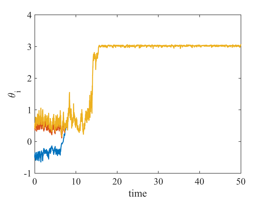
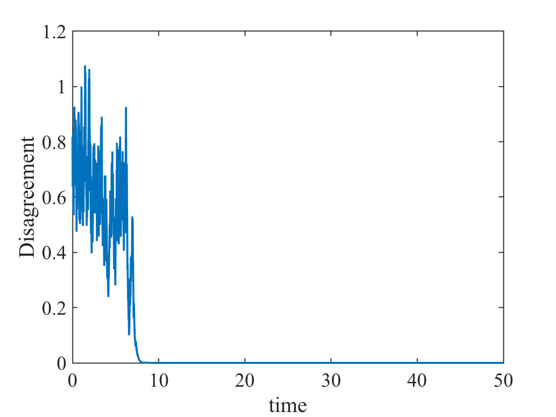
(b) $\sigma=1$

Figure 1: (a) In the absence of a common noise, the oscillators do not synchronize. (b) Addition of common noise enables synchronization of oscillators.

3 Phase reduction: A short review

3.1 Phase reduction for deterministic oscillators

In this section we first review the phase reduction technique for oscillators. Consider the autonomous system

$$\dot{x}=F(x),\quad x\in\mathbb{R}^{m},\quad m\geq 2,$$ (30)

with an asymptotically stable hyperbolic limit cycle $x^{\gamma}(t)$ of period $T$ and frequency $\omega=\frac{2\pi}{T}$. The phase of an oscillator, denoted by $\theta(t)$, is the time that has elapsed as its state moves around the limit cycle $x^{\gamma}(t)$, starting from an arbitrary reference point $\bar{\theta}$ on the cycle, called relative phase. The phase, defined by $\theta(t)=\omega t+\bar{\theta}\quad(\mbox{mod}\;2\pi)$, reduces the dynamics of (30) to the following scalar phase equation

$$\dot{\theta}(t)=\omega.$$

There is a one to one correspondence between phase $\theta$ and each point $x$ on the limit cycle $x^{\gamma}(t)$. This correspondence defines the following phase map [13, 14] on the basin of attraction of $x^{\gamma}(t)$:

$$\Phi(x(t)):=\theta(t)=\omega t+\bar{\theta},\quad x\in x^{\gamma},$$

with dynamics

$$\dot{\Phi}(x(t))=\nabla\Phi(x)\cdot\dot{x}=\nabla\Phi(x)\cdot F(x)=\omega,\quad x\in x^{\gamma},$$ (31)

where $\cdot$ denotes the inner product.

We now consider the effect of small perturbations to the dynamics of (30), which no longer leave $x^{\gamma}(t)$ invariant. To this end, we first generalize the definition of the phase map to a neighborhood of $x^{\gamma}(t)$. Since $x^{\gamma}(t)$ is asymptotically stable, for any point $y$ in the basin of attraction of $x^{\gamma}(t)$, there exists an $x\in x^{\gamma}(t)$ such that as $t\to\infty$, $\|X(t,x)-X(t,y)\|\to 0$, where $X(\cdot,x)$ is the unique solution of (30) with initial condition $x$, and $\|\cdot\|$ is an arbitrary norm in $\mathbb{R}^{n}$. The set of all such points $y$ is called the isochron of $x$. For any $x\in x^{\gamma}$, all the points on the isochron of $x$ have the same phase as $x$, i.e., $\Phi$ can be extended to the basin of attraction of $x^{\gamma}$ as follows:

$$\Phi(y):=\Phi(x)=\theta,\quad\forall y\in\mbox{isochron of $x$}.$$

Note that the isochron of $x$ is a level set of $\Phi(x)$.

Now consider (30) with a small perturbation $G$, which could describe the coupling to other oscillators.

$$\dot{x}=F(x)+\epsilon G(x,\ldots),\quad x\in\mathbb{R}^{m},\quad 0<\epsilon\ll 1.$$ (32)

Then, using (31), we have

$$\dot{\Phi}(x(t))=\nabla\Phi\cdot\dot{x}=\nabla\Phi\cdot(F+\epsilon G)=\omega+\epsilon\;\nabla\Phi\cdot G.$$

Therefore, by definition of the phase map, the dynamics of (32) can be reduced to the following phase equation

$$\dot{\theta}=\omega+\epsilon\;\nabla\Phi\cdot G.$$

The gradient of the phase map, $\nabla\Phi$, called the phase response curve (PRC) and captures changes in the phase per unit perturbation for small perturbations, plays an important role in reducing the system (32). In this work, we also use the Hessian of the phase map. To distinguish between the gradient and the Hessian, we refer to the gradient as the first-order PRC and the Hessian as the second-order PRC. In what follows, we review two essential methods to compute first-order PRCs.

3.2 Computation of first-order phase response curves

The first-order PRC, denoted by $\boldsymbol{Z}(\theta)$, is defined by the gradient of the phase map $\nabla\Phi(x)$ at the point on the limit cycle associated with phase $\theta$. The first-order PRC can be computed using a direct method in which a perturbation is introduced at each point of the limit cycle and the resulting change in phase is recorded,

$$\boldsymbol{Z}_{i}(\theta)=\frac{\partial\Phi}{\partial x_{i}}({x})=\lim_{r\to 0}\frac{1}{r}\left(\Phi({x}+r\hat{i})-\Phi(x)\right),\quad x\in x^{\gamma},$$

where $\hat{i}$ is the $i$-th coordinate vector.

Alternatively, the adjoint method can be used that solves the following ODE in reverse time [6, 10]

$$\frac{d}{dt}\nabla{\Phi}(x^{\gamma}(t))=-DF^{\top}(x^{\gamma}(t))\nabla{\Phi}(x^{\gamma}(t)),$$ (33)

with constraint

$$\nabla{\Phi}(x^{\gamma}(0))\cdot F(x^{\gamma}(0))=\omega,$$ (34)

where $DF^{\top}$ denotes the transpose of the Jacobian of $F$. Note that due to the negative sign in front of $-DF^{\top}$, the stability of the adjoint equation (33) is the opposite of the stability of the limit cycle. Hence, the adjoint equation needs to be solved in reverse time.

4 Phase reduction for a single noisy oscillator

We now focus on the effect of noise in the dynamics of equation (30) and its phase reduction. Consider (30) with multiplicative white noise

$$dx=F(x)dt+\sigma K(x)dW(t),$$ (35)

where $K(x)\in\mathbb{R}^{m\times m}$ is the diffusion matrix, $0<\sigma\ll 1$ is a constant determining the intensity of noise, and $dW(t)$ is a standard $m$-dimensional Weiner process increment. We could equivalently write the corresponding Langevin system

$$\dfrac{d{x}}{dt}=F(x)+\sigma K(x)\xi(t),$$

where $\xi$ is $m-$dimensional white Gaussian noise. Therefore, we interpret (35) in Itô sense.

In the absence of noise, $\sigma=0$, the SDE (35) becomes an ODE $\dot{x}=F(x)$, that we assume it admits an asymptotically stable limit cycle $x^{\gamma}(t)$ with time period $T$ and frequency $\omega=\frac{2\pi}{T}$. We denote $x^{\gamma}(t)$ by $\gamma(\theta(t))=\gamma(\omega t+\psi(t))$, where $\theta(t)$ and $\psi(t)$ are the asymptotic phase and relative phase, respectively. By a noisy oscillator, denoted by $x(t)$, we mean the solution of (35) which can be approximated by $x^{\gamma}(t)$ for sufficiently small $\sigma$.

Before we discuss the phase reduction of noisy oscillators, we first introduce the second-order PRC, denoted by $\boldsymbol{H}(\theta)$ and defined by the Hessian of the phase map $\nabla^{2}\Phi(x)$ at the point on the limit cycle associated with phase $\theta$. In Section 4.1, we will discuss the second-order PRC in details.

Proposition 1 (Phase reduction of noisy oscillators).

For the noisy oscillator (35), the dynamics of the phase in a neighborhood of the limit cycle is

$$d\theta=\Big{(}\omega+\frac{\sigma^{2}}{2}\mathrm{tr}\big{[}K(\gamma(\theta))^{\top}\boldsymbol{H}(\theta)K(\gamma(\theta))\big{]}\Big{)}dt+\sigma\boldsymbol{Z}(\theta)^{\top}K(\gamma(\theta))dW(t).$$ (36)

Proof.

since we interpret (35) in Itô sense, we apply the Itô chain rule [41, Theorem 4.16] to the phase map $\Phi(x(t))$ to obtain

$$d\Phi(x) =\nabla\Phi(x)\cdot F(x)dt+\sigma\nabla\Phi(x)\cdot K(x)dW(t)$$

$$\quad+\frac{1}{2}\big{(}F(x)dt+\sigma K(x)dW(t)\big{)}^{\top}\nabla^{2}\Phi(x)\big{(}F(x)dt+\sigma K(x)dW(t)\big{)}$$

$$\approx\nabla\Phi(x^{\gamma})\cdot F(x^{\gamma})dt+\sigma\nabla\Phi(x^{\gamma})\cdot K(x^{\gamma})dW(t)$$

$$\quad+\frac{1}{2}\big{(}F(x^{\gamma})dt+\sigma K(x^{\gamma})dW(t)\big{)}^{\top}\nabla^{2}\Phi(x^{\gamma})\big{(}F(x^{\gamma})dt+\sigma K(x^{\gamma})dW(t)\big{)}$$

$$=\Big{(}\omega+\frac{\sigma^{2}}{2}\mathrm{tr}\big{[}K(x^{\gamma})^{\top}\nabla^{2}\Phi(x^{\gamma})K(x^{\gamma})\big{]}\Big{)}dt+\sigma\nabla\Phi(x^{\gamma})\cdot K(x^{\gamma})dW(t),$$

which yields the desired result similar to [41, Theorem 4.16]. ∎

Note that the phase equation derived in Proposition 1 is different from the existing phase equations (using PRC approach), e.g., [28] and [29, 17]. Our approach to compute $d\theta$ is to interpret the SDEs in Itô and employ Itô chain rule, while in the literature, the SDEs are interpreted in Stratonovich and after computing $d\theta$ using ordinary chain rules, they are transferred to SDEs in the Itô sense. In an Appendix we provide a few examples which explain the difference between the two approaches.

Remark 2.

If $K(x)$ is the identity, (36) reduces to

$$d\theta=\Big{(}\omega+\frac{\sigma^{2}}{2}\sum_{i=1}^{n}\boldsymbol{H}_{ii}(\theta)\Big{)}dt+\sigma\boldsymbol{Z}(\theta)^{\top}dW(t),$$ (37)

where $\boldsymbol{H}_{ii}$s are the diagonal entries of $\boldsymbol{H}$.

Example 2.

(Phase reduction of noisy Hopf bifurcation normal form.) We consider the normal form of a supercritical Hopf bifurcation with additive noise:

$$\begin{split}dx_{1}&=(\mu x_{1}-\omega x_{2}-(x_{1}^{2}+x_{2}^{2})x_{1})dt+\sigma dW_{1}(t),\\ dx_{2}&=(\omega x_{1}+\mu x_{2}-(x_{1}^{2}+x_{2}^{2})x_{2})dt+\sigma dW_{2}(t).\end{split}$$ (38)

Recall that, without noise, the dynamics of (38) yields a circular limit cycle centered at the origin with radius $\sqrt{\mu}$ and frequency $\omega$. Furthermore, given the phase $\theta$ on the limit cycle, the associated point $(x_{1}^{\gamma},x_{2}^{\gamma})=(\sqrt{\mu}\cos(\theta),\sqrt{\mu}\sin(\theta))$. Equivalently, $\theta=\Phi(x_{1}^{\gamma},x_{2}^{\gamma})=\tan^{-1}(x_{2}^{\gamma}/x_{1}^{\gamma})$. It follows immediately that

$$\begin{split}\boldsymbol{Z}(\theta)=\frac{1}{\sqrt{\mu}}\left(\begin{array}[]{cc}-\sin(\theta)\\ \cos(\theta)\end{array}\right),\quad\boldsymbol{H}(\theta)=\frac{1}{\mu}\left(\begin{array}[]{cccc}\sin(2\theta)&-\cos(2\theta)\\ -\cos(2\theta)&-\sin(2\theta)\end{array}\right).\end{split}$$ (39)

Therefore, using (37), the phase reduction for the noisy Hopf bifurcation normal form (38) is

$$d\theta=\omega dt+\frac{\sigma}{\sqrt{\mu}}dW(t).$$

4.1 Computation of second-order phase response curves

The Hessian of the phase map, denoted by $\boldsymbol{H}(\theta(t))=\nabla^{2}\Phi(x(t))$ and called the second-order PRC, plays an important role in phase reduction of stochastic oscillators [42, 25, 43]. Similar to the first-order PRC, the second-order PRC can be computed using a direct method as follows.

$$\boldsymbol{H}_{ij}(\theta)=\frac{\partial^{2}\Phi}{\partial x_{i}\partial x_{j}}(x)=\lim_{r\to 0}\frac{1}{r}\left(\dfrac{\partial\Phi}{\partial x_{j}}(x+r\hat{i})-\dfrac{\partial\Phi}{\partial x_{j}}(x)\right).$$

Note that for an identity diffusion matrix $K$, one only needs to compute the diagonal entries of $\boldsymbol{H}$, as follows (without computing the first-order PRC).

$$\boldsymbol{H}_{ii}(\theta)=\lim_{r\to 0}\frac{1}{r}\left(\Phi(x+r\hat{i})-2\Phi(x)+\Phi(x-r\hat{i})\right).$$

Alternatively, the second-order PRC solves the following ODE in reverse time

$$\dot{\boldsymbol{H}}(\theta)=-\nabla^{2}{F}(\boldsymbol{Z}(\theta)\otimes{I})-DF^{\top}\boldsymbol{H}(\theta)-\boldsymbol{H}(\theta)DF,$$ (40)

where all the arguments $(x^{\gamma}(t))$ from $\nabla^{2}F$ and $DF$ are dropped; $\nabla^{2}F=[\nabla^{2}F_{1}\cdots\nabla^{2}F_{n}]$ is an $m\times m^{2}$ matrix and represents the Hessian matrix of the vector field $F$, $\otimes$ is the Kronecker product and $I$ is the $m\times m$ identity matrix. The initial condition is determined by the following constraint

$$F^{\top}(x^{\gamma}(0))\boldsymbol{H}(\theta)F(x^{\gamma}(0))=-\left(F^{\top}DF^{\top}\right)(x^{\gamma}(0))\boldsymbol{Z}(\theta).$$ (41)

Proposition 2 (Computing the second-order PRC).

Consider system (30) with an asymptotically stable limit cycle $x^{\gamma}(t)$ and its corresponding phase map $\Phi$. Let $\nabla^{2}\Phi$ be the Hessian matrix of the phase map $\Phi$. Then $\nabla^{2}\Phi$ solves (40) with constraint (41). $\square$

Proof.

Let $x^{\gamma}_{p}(t):=x^{\gamma}(t)+r{p}(t)$ be a solution of (30) which starts at $x^{\gamma}_{p}(0):=x^{\gamma}(0)+r{\boldsymbol{p}}(0)$, where $0<r\ll 1$ and ${p}(t)$ represent the magnitude and the direction of the perturbation, respectively. Since $r{p}(0)$ is very small and $x^{\gamma}(t)$ is asymptotically stable, for any $t>0$, $rp(t)$ remains small and it therefore satisfies, including $\mathcal{O}(r^{2})$ terms

$$\begin{split}&r\dot{p}(t)=\boldsymbol{F}(x^{\gamma}(t)+r{p}(t))-F(x^{\gamma}(t))\\ \ &=\left(\begin{array}[]{ccc}r\boldsymbol{p}(t)^{\top}\nabla\boldsymbol{F}_{1}(\boldsymbol{x}^{\gamma}(t))+\dfrac{r^{2}}{2}\boldsymbol{p}(t)^{\top}\nabla^{2}\boldsymbol{F}_{1}(\boldsymbol{x}^{\gamma}(t))\boldsymbol{p}(t)\\ \vdots\\ r\boldsymbol{p}(t)^{\top}\nabla\boldsymbol{F}_{n}(\boldsymbol{x}^{\gamma}(t))+\dfrac{r^{2}}{2}\boldsymbol{p}(t)^{\top}\nabla^{2}\boldsymbol{F}_{n}(\boldsymbol{x}^{\gamma}(t))\boldsymbol{p}(t)\end{array}\right)\\ &=rD{\boldsymbol{F}}(\boldsymbol{x}^{\gamma}(t)){\boldsymbol{p}}(t)+\dfrac{r^{2}}{2}\left(\begin{array}[]{ccc}\boldsymbol{p}(t)^{\top}\nabla^{2}\boldsymbol{F}_{1}(\boldsymbol{x}^{\gamma}(t))\boldsymbol{p}(t)\\ \vdots\\ \boldsymbol{p}(t)^{\top}\nabla^{2}\boldsymbol{F}_{n}(\boldsymbol{x}^{\gamma}(t))\boldsymbol{p}(t)\end{array}\right).\end{split}$$ (42)

Let $\Delta\theta:=\Phi(\boldsymbol{x}^{\gamma}_{p}(t))-\Phi(\boldsymbol{x}^{\gamma}(t))$ be the phase difference of $\boldsymbol{x}^{\gamma}(t)$ and its perturbation $\boldsymbol{x}^{\gamma}_{p}(t)$. Then the Taylor expansion of $\Phi$ at $\boldsymbol{x}^{\gamma}(t)$ gives, up to $\mathcal{O}(r^{2})$:

$$\begin{split}\Delta\theta&=\Phi(\boldsymbol{x}^{\gamma}_{p}(t))-\Phi(\boldsymbol{x}^{\gamma}(t))\\ &=\Phi(\boldsymbol{x}^{\gamma}+r{\boldsymbol{p}}(t))-\Phi(\boldsymbol{x}^{\gamma}(t))\\ &=r{\boldsymbol{p}}(t)^{\top}\nabla\Phi(\boldsymbol{x}^{\gamma}(t))+\dfrac{r^{2}}{2}{\boldsymbol{p}}(t)^{\top}\nabla^{2}\Phi(\boldsymbol{x}^{\gamma}(t)){\boldsymbol{p}}(t).\end{split}$$ (43)

Note that since the limit cycle is asymptotically stable and the perturbation is small enough such that $\boldsymbol{x}_{p}^{\gamma}(t)$ remains within the basin of attraction of $\boldsymbol{x}^{\gamma}(t)$, although the phases of $\boldsymbol{x}^{\gamma}(t)$ and $\boldsymbol{x}^{\gamma}_{p}(t)$ change with time, their difference remains constant. Therefore, taking the time derivative of both sides of (43), and dropping the arguments $t$ from $\boldsymbol{p}$ and $\boldsymbol{x}^{\gamma}(t)$ from $\nabla^{2}\boldsymbol{F}_{i}$, $\nabla\Phi$ and $\nabla^{2}\Phi,$ we get

$$\begin{split}0&=r\left[\dot{\boldsymbol{p}}^{\top}\nabla\Phi+{\boldsymbol{p}}^{\top}\dfrac{d}{dt}\nabla\Phi\right]\\ &+\dfrac{r^{2}}{2}\left[\dot{\boldsymbol{p}}^{\top}\nabla^{2}\Phi\;{\boldsymbol{p}}+{\boldsymbol{p}}^{\top}\frac{d}{dt}\nabla^{2}\Phi\;{\boldsymbol{p}}+{\boldsymbol{p}}^{\top}\nabla^{2}\Phi\;\dot{\boldsymbol{p}}\right].\end{split}$$ (44)

Substituting (42) into (44) and dropping the argument $\boldsymbol{x}^{\gamma}(t)$ from $D{\boldsymbol{F}}$, we get

$$\begin{split}0&=r\left[{\boldsymbol{p}}^{\top}D{\boldsymbol{F}}^{\top}\nabla\Phi+{\boldsymbol{p}}^{\top}\dfrac{d}{dt}\nabla\Phi\right]+\dfrac{r^{2}}{2}\left(\begin{array}[]{ccc}\boldsymbol{p}^{\top}\nabla^{2}\boldsymbol{F}_{1}\boldsymbol{p}\\ \vdots\\ \boldsymbol{p}^{\top}\nabla^{2}\boldsymbol{F}_{n}\boldsymbol{p}\end{array}\right)\cdot\nabla\Phi\\ &+\dfrac{r^{2}}{2}\left[{\boldsymbol{p}}^{\top}D{\boldsymbol{F}}^{\top}\nabla^{2}\Phi\;{\boldsymbol{p}}+{\boldsymbol{p}}^{\top}\frac{d}{dt}\nabla^{2}\Phi\;{\boldsymbol{p}}+{\boldsymbol{p}}^{\top}\nabla^{2}\Phi\;D{\boldsymbol{F}}{\boldsymbol{p}}\right]\\ &=r{\boldsymbol{p}}^{\top}\left[D{\boldsymbol{F}}^{\top}\nabla\Phi+\dfrac{d}{dt}\nabla\Phi\right]+\dfrac{r^{2}}{2}{\boldsymbol{p}}^{\top}\times\\ &\left[\nabla^{2}{\bf F}(\nabla\Phi\otimes{\boldsymbol{I}})+D{\boldsymbol{F}}^{\top}\nabla^{2}\Phi\;+\frac{d}{dt}\nabla^{2}\Phi\;+\nabla^{2}\Phi\;D{\boldsymbol{F}}\right]{\boldsymbol{p}}.\end{split}$$ (45)

Since (45) holds for any arbitrary small perturbation, the following two equations must hold:

$$\dfrac{d}{dt}\nabla\Phi=-D{\boldsymbol{F}}^{\top}\nabla\Phi,$$ (46)

which is the adjoint equation (33) for the PRC; and

$$\dfrac{d\nabla^{2}\Phi}{dt}=-\nabla^{2}{\bf F}(\nabla\Phi\otimes{\boldsymbol{I}})-D{\boldsymbol{F}}^{\top}\nabla^{2}\Phi-\nabla^{2}\Phi\;D{\boldsymbol{F}},$$ (47)

which is the ODE (40), after replacing $\nabla^{2}\Phi$ by $H$ and $\nabla\Phi$ by $\boldsymbol{Z}$. Next we show that (41) holds. To this end, we take the second time derivative of the phase map $\Phi(\boldsymbol{x}^{\gamma}(t))=\theta(t)=\omega t+\bar{\theta}$ and evaluate it at $\boldsymbol{x}^{\gamma}(0)$. The first derivative gives

$$\dfrac{d\Phi}{dt}(\boldsymbol{x}^{\gamma}(t))=\boldsymbol{F}^{\top}\nabla\Phi=\omega.$$ (48)

Note that this equation guarantees the constraint (34) for the PRC. Taking another time derivative of (48) yields

$$\dfrac{d^{2}\Phi}{dt^{2}}=\boldsymbol{F}^{\top}\nabla^{2}\Phi\boldsymbol{F}+\boldsymbol{F}^{\top}D\boldsymbol{F}^{\top}\nabla\Phi=0.$$ (49)

Note that the second term of the sum holds because by the chain rule,

$$\dfrac{d}{dt}\boldsymbol{F}(\boldsymbol{x}^{\gamma}(t)) =\frac{\partial\boldsymbol{F}}{\partial\boldsymbol{x}}(\boldsymbol{x}^{\gamma}(t))\frac{d\boldsymbol{x}^{\gamma}}{dt}(t)$$ (50)

$$=D\boldsymbol{F}(\boldsymbol{x}^{\gamma}(t))\boldsymbol{F}(\boldsymbol{x}^{\gamma}(t)).$$

Therefore, for any time $t$

$$(\boldsymbol{F}^{\top}\nabla^{2}\Phi\boldsymbol{F})(\boldsymbol{x}^{\gamma}(t)) =-(\boldsymbol{F}^{\top}D\boldsymbol{F}^{\top}\nabla\Phi)(\boldsymbol{x}^{\gamma}(t)).$$

and in particular at $t=0$, after replacing $\nabla^{2}\Phi(\boldsymbol{x}^{\gamma}(0))$ by $H(\bar{\theta})$ and $\nabla\Phi(\boldsymbol{x}^{\gamma}(0))$ by $\boldsymbol{Z}(\bar{\theta})$, we get the desired constraint, (41). ∎

A proof of Proposition 2 can be found in [44, Section 2].

Remark 3.

The following choices of initial conditions for $\nabla\Phi$ and $\nabla^{2}\Phi$ guarantee the constraints given in (34) and (41), respectively:

$$\nabla\Phi(x^{\gamma}(0)) =\dfrac{\omega}{(F^{\top}F)(x^{\gamma}(0))}F(x^{\gamma}(0)),$$

$$\nabla^{2}\Phi(x^{\gamma}(0)) =-\dfrac{\omega}{2(F^{\top}F)(x^{\gamma}(0))}(DF+DF^{\top})(x^{\gamma}(0)).$$

Remark 4.

In what follows, we vectorize [45] equation (40) and combine the corresponding equations of the first- and second-order PRC. Let $\boldsymbol{H}_{v}=\text{vec}(\boldsymbol{H})$ be the vectorization of $\boldsymbol{H}$, i.e., the vector of the columns of $\boldsymbol{H}$. Then,

$$\begin{split}\dot{\boldsymbol{Z}}&=-DF^{\top}\boldsymbol{Z},\\ \dot{\boldsymbol{H}}_{v}&=-(I\otimes DF^{\top}+DF^{\top}\otimes I)\boldsymbol{H}_{v}-(I\otimes\nabla^{2}F)\text{vec}({\boldsymbol{Z}\otimes I}),\\ &=-(I\otimes DF^{\top}+DF^{\top}\otimes I)\boldsymbol{H}_{v}-({\boldsymbol{Z}^{\top}\otimes I\otimes I})\text{vec}(\nabla^{2}F),\end{split}$$ (51)

with constraints

$$F^{\top}(x^{\gamma}(0))\boldsymbol{Z}(0) =\omega,$$

$$(F^{\top}\otimes F^{\top})(x^{\gamma}(0))\boldsymbol{H}_{v}(0) =\left(F^{\top}DF^{\top}\boldsymbol{Z}\right)(x^{\gamma}(0)),$$

where the following vectorization equalities are used for arbitrary matrices $A$, $B$, and $C$:

$$\text{vec}(AB) =(I\otimes A)\text{vec}(B)=(B^{\top}\otimes I)\text{vec}(A),$$

$$\text{vec}(ABC) =(C^{\top}\otimes A)\text{vec}(B).$$

Here $I$ is an identity matrix of the appropriate size.

Remark 5.

Due to the negative sign in the right hand side of (40), or equivalently (51), its stability is the opposite of the stability of the limit cycle. Hence, the equation needs to be solved in reverse time.

Example 3.

(Hopf bifurcation normal form.) For the Hopf bifurcation dynamics (38) with $\sigma=0$, it can be verified that the matrix $\boldsymbol{H}$ derived in (39) satisfies (40).

Example 4.

(Van der Pol oscillator.) We now consider the van der Pol oscillator with additive white noise

$$dx_{1} =\left(x_{1}-\frac{1}{3}x_{1}^{3}-x_{2}\right)dt+\sigma dW_{1}(t)$$ (52a)

$$dx_{2} =x_{1}dt+\sigma dW_{2}(t).$$ (52b)

Figure 2 shows the first-order PRC and the second-order PRC for dynamics (52) with $\sigma=0$. These 2-component PRCs are computed by numerically solving (51) with initial conditions discussed in Remark 3.

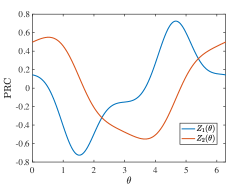
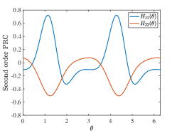
Figure 2: The components of the first-order PRC (left) and the second-order PRC (right) of the Van der Pol oscillator.

5 Phase reduction of weakly coupled noisy oscillators

In this section, we derive coupled phase equations of a network of noisy oscillators which are weakly connected through noisy interactions. For $i=1,\ldots,N$, let

$$d{x_{i}}=\underbrace{F(x_{i})dt+\sigma K(x_{i})dW_{i}(t)}_{\text{intrinsic dynamics}}\;+\;\underbrace{\sum_{j=1}^{N}c_{ij}\big{(}\epsilon H(x_{j},x_{i})dt+\delta C(x_{j},x_{i})dW_{ij}(t)\big{)}}_{\text{coupling dynamics}}$$ (53)

describe the dynamics of each oscillator $i$ and its interaction with its adjacent oscillators, the set of oscillators which are connected to $i$. The set up of (53) is very similar to (1): There is an underlying weighted graph with weight $c_{ij}$ which does not need to be undirected, i.e., $c_{ij}\neq c_{ji}$.

The first two terms describe the dynamics of each isolated oscillator as discussed in (35). We assume that the oscillators have identical dynamics and allow small common noise on their dynamics. The noise can arise from a noisy environment, which affects the dynamics of each individual, or the intrinsic property of the agents. In terms of modeling, one may assume that the model parameters are buried in noise. The last two terms of (53) describe the noisy interactions between oscillator $i$ and its adjacent oscillators. This noise arises from the edges of the graph.

In (53), the state variable $x_{i}$, the internal dynamics $F(x_{i})$, and the deterministic interaction function $H(x_{j},x_{i})$ are $m-$dimensional vectors. The $m\times m$ diffusion matrices $\sigma K$ and $\delta C$ describe the correlation of common noise and interaction noise, respectively. The vectors $dW_{i}$ and $dW_{ij}$ are $m-$dimensional standard Wiener process increments, i.e., $\langle dW_{i}^{k}(t),dW_{i}^{l}(s)\rangle=\delta_{kl}(t-s)$, where $dW_{i}^{k}$ is the $k-$th argument of $dW_{i}$. Similarly, $\langle dW_{ij}^{k}(t),dW_{ij}^{l}(s)\rangle=\delta_{kl}(t-s)$, where $dW_{ij}^{k}$ is the $k-$th argument of $dW_{ij}$.

The constant parameters $\epsilon$, $\sigma$, and $\delta$, which respectively represent the deterministic coupling strength, the common and interaction noise intensities, are assumed to be sufficiently small and satisfy

$$\mathcal{O}(\sigma)=\mathcal{O}(\delta)=\mathcal{O}(\sqrt{\epsilon}),\qquad 0<\epsilon\ll 1.$$ (54)

For $\epsilon=\sigma=\delta=0$, (53) reduces to $\dot{x}_{i}=F(x_{i})$, that we assume admits an asymptotically stable limit cycle $x_{i}^{\gamma}$ with frequency $\omega$. We denote $x_{i}^{\gamma}$ by $\gamma(\theta_{i}(t))=\gamma(\omega t+\psi_{i}(t))$, where $\theta_{i}$ and $\psi_{i}$ are respectively the asymptotic phase and relative phase of oscillator $i$.

A solution of (53), denoted by $x_{i}(t)$, is called a noisy oscillator. Note that we assume that $\epsilon$, $\sigma$, and $\delta$ are small enough so that the trajectories stay within the basin of attraction of the limit cycles $x_{i}^{\gamma}$ after receiving the deterministic and stochastic perturbations. We also assume that $x_{i}$ can be approximated by $x_{i}^{\gamma}$.

Proposition 3 (Phase reduction of weakly coupled noisy oscillators).

For the noisy coupled oscillators (53), the dynamics of the coupled phases $\theta_{i}$ in neighborhoods of the limit cycles are

$$d\theta_{i} =\left(\omega+\epsilon\sum_{j}c_{ij}\boldsymbol{Z}^{\top}H+\frac{\sigma^{2}}{2}\mathrm{tr}[K^{\top}\boldsymbol{H}K]+\frac{\delta^{2}}{2}\mathrm{tr}\Big{[}\sum_{j}c_{ij}^{2}C^{\top}\boldsymbol{H}C\Big{]}\right)\;dt$$

$$\quad+\sigma\boldsymbol{Z}^{\top}K\;dW_{i}(t)+\delta\sum_{j}c_{ij}\boldsymbol{Z}^{\top}C\;dW_{ij}(t),$$ (55)

where $\boldsymbol{Z}=\boldsymbol{Z}(\theta_{i})$, $\boldsymbol{H}=\boldsymbol{H}(\theta_{i})$, $H=H(\gamma(\theta_{j}),\gamma(\theta_{i}))$, $K=K(\gamma(\theta_{i}))$, $C=C(\gamma(\theta_{j}),\gamma(\theta_{i}))$, and $\sum_{j}=\sum_{j=1}^{N}$.

Note that we use $H$ for the coupling function and $\boldsymbol{H}$ for the second-order PRC.

Proof.

We apply the Itô formula [41, Theorem 4.16] to the phase map $\Phi(x_{i}(t))$. Then

$$d\Phi(x_{i}) =\nabla\Phi(x_{i})\cdot\Big{[}F(x_{i})+\epsilon\sum_{j}c_{ij}H(x_{j},x_{i})\Big{]}dt$$

$$\quad+\nabla\Phi(x_{i})\cdot\Big{(}\sigma K(x_{i})dW_{i}(t)+\delta\sum_{j}c_{ij}C(x_{j},x_{i})dW_{ij}(t)\Big{)}$$

$$\quad+\frac{1}{2}\Big{[}F(x_{i})dt+\epsilon\sum_{j}c_{ij}H(x_{j},x_{i})dt+\sigma K(x_{i})dW_{i}(t)+\delta\sum_{j}c_{ij}C(x_{j},x_{i})dW_{ij}(t)\Big{]}^{\top}$$

$$\qquad\nabla^{2}\Phi(x_{i})\Big{[}F(x_{i})dt+\epsilon\sum_{j}c_{ij}H(x_{j},x_{i})dt+\sigma K(x_{i})dW_{i}(t)+\delta\sum_{j}c_{ij}C(x_{j},x_{i})dW_{ij}(t)\Big{]}$$

$$=\nabla\Phi(x_{i})\cdot\Big{[}F(x_{i})+\epsilon\sum_{j}c_{ij}H(x_{j},x_{i})\Big{]}dt$$

$$\quad+\nabla\Phi(x_{i})\cdot\Big{(}\sigma K(x_{i})dW_{i}(t)+\delta\sum_{j}c_{ij}C(x_{j},x_{i})dW_{ij}(t)\Big{)}$$

$$\quad+\frac{1}{2}\mathrm{tr}\Big{[}\sigma^{2}K(x_{i})^{\top}\nabla^{2}\Phi(x_{i})K(x_{i})+\delta^{2}\sum_{j}c_{ij}^{2}C(x_{j},x_{i})^{\top}\nabla^{2}\Phi(\boldsymbol{x}_{i})C(x_{j},x_{i})\Big{]}dt$$

$$\approx\nabla\Phi(x_{i}^{\gamma})\cdot\Big{[}F(x_{i}^{\gamma})+\epsilon\sum_{j}c_{ij}H(x_{j}^{\gamma},x_{i}^{\gamma})\Big{]}dt$$

$$\quad+\nabla\Phi(x_{i}^{\gamma})\cdot\Big{(}\sigma K(x_{i}^{\gamma})dW_{i}(t)+\delta\sum_{j}c_{ij}C(x_{j}^{\gamma},x_{i}^{\gamma})dW_{ij}(t)\Big{)}$$

$$\quad+\frac{1}{2}\mathrm{tr}\Big{[}\sigma^{2}K(x_{i}^{\gamma})^{\top}\nabla^{2}\Phi(x_{i}^{\gamma})K(x_{i}^{\gamma})+\delta^{2}\sum_{j}c_{ij}^{2}C(x_{j}^{\gamma},x_{i}^{\gamma})^{\top}\nabla^{2}\Phi(x_{i}^{\gamma})C(x_{j}^{\gamma},x_{i}^{\gamma})\Big{]}dt$$

$$=\Big{[}\omega+\epsilon\sum_{j}c_{ij}\nabla\Phi(x_{i}^{\gamma})\cdot H(x_{j}^{\gamma},x_{i}^{\gamma})\Big{]}dt$$

$$\quad+\frac{1}{2}\mathrm{tr}\Big{[}\sigma^{2}K(x_{i}^{\gamma})^{\top}\nabla^{2}\Phi(x_{i}^{\gamma})K(x_{i}^{\gamma})+\delta^{2}\sum_{j}c_{ij}^{2}C(x_{j}^{\gamma},x_{i}^{\gamma})^{\top}\nabla^{2}\Phi(x_{i}^{\gamma})C(x_{j}^{\gamma},x_{i}^{\gamma})\Big{]}dt$$

$$\quad+\nabla\Phi(x_{i}^{\gamma})\cdot\Big{(}\sigma K(x_{i}^{\gamma})dW_{i}(t)+\delta\sum_{j}c_{ij}C(x_{j}^{\gamma},x_{i}^{\gamma})dW_{ij}(t)\Big{)},$$

which yields the desired result. The first equality is obtained by the Itô formula, the second equality obtained from the equalities $dt\cdot dt=dt\cdot dW_{i}=dt\cdot dW_{ij}=dW_{ij}\cdot dW_{i}=0$ and $dW_{i}\cdot dW_{i}=dW_{ij}\cdot dW_{ik}=\delta_{jk}dt$. The approximation is obtained by the assumption that each noisy oscillator $x_{i}$ can be approximated by $x_{i}^{\gamma}$, and the last equality obtained from $\nabla\Phi(x_{i}^{\gamma})\cdot F(x_{i}^{\gamma})=\omega$. ∎

6 Stochastic synchronization of coupled phase reduced equations

In this section, we apply Theorems 1 and 2 (and similarly Theorem 3) to the coupled phase equations (3) and, based on the given PRCs, $\boldsymbol{Z}$ and $\boldsymbol{H}$, we will design appropriate $K,H,$ and $C$ that guarantee the oscillators’ synchronization.

In what follows, we consider three separate cases: (1) no edge coupling, (2) deterministic edge coupling, and (3) stochastic edge coupling.

Case 1. No edge coupling. First, we consider $N$ oscillators which are connected only through a common noise, i.e., consider (3) with no coupling ($c_{ij}=c_{ji}=0$) and $dW_{i}=d\hat{W}$, where $d\hat{W}$ is an $m-$dimensional Wiener increment.

$$d\theta_{i} =\left(\omega+\frac{\sigma^{2}}{2}\mathrm{tr}[K^{\top}\boldsymbol{H}K]\right)\;dt+\sigma\boldsymbol{Z}^{\top}K\;d\hat{W}(t),$$ (56)

and check conditions (i) and (iv) of Theorem 1 and condition (ii) of Theorem 2. To apply these theorem, (56) must be in the format of (1), with a $1-$dimensional Wiener increment. To this end, we write $\sigma\boldsymbol{Z}^{\top}K\;d\hat{W}(t)$ as $\sigma\mathcal{K}\;dW(t)$ where $\mathcal{K}=\sqrt{\boldsymbol{Z}^{\top}KK^{\top}\boldsymbol{Z}}$ is a scalar and $dW$ is a $1-$dimensional Wiener increment.

$$d\theta_{i} =\left(\omega+\frac{\sigma^{2}}{2}\mathrm{tr}[K^{\top}\boldsymbol{H}K]\right)\;dt+\sigma\mathcal{K}\;dW(t).$$ (57)

Condition i of Theorem 1.

Assume that $K$ is differentiable and let

$$\bar{c}_{\mathcal{F}}:=\dfrac{\sigma^{2}}{2}{\sup_{(\phi,t)\in(-\frac{\pi}{2},\frac{\pi}{2})\times[0,T)}}\lambda_{\max}\left[\frac{\partial}{\partial\phi}\Big{(}K(\gamma(\omega t+\phi))^{\top}\boldsymbol{H}(\omega t+\phi)K(\gamma(\omega t+\phi))\Big{)}\right],$$ (58)

where $\lambda_{\max}[A]$ denotes the maximum eigenvalue of $A$. Then, for $\phi,\eta\in{(-\frac{\pi}{2},\frac{\pi}{2})}$ and $t\in[0,T)$:

$$(\phi-\eta)(\mathcal{F}(\phi,t)-\mathcal{F}(\eta,t))\leq\bar{c}_{\mathcal{F}}(\phi-\eta)^{2},$$

where $\mathcal{F}(\phi,t)=\omega+\frac{\sigma^{2}}{2}\mathrm{tr}[K(\gamma(\omega t+\phi))^{\top}\boldsymbol{H}(\omega t+\phi)K(\gamma(\omega t+\phi))].$ We used $\mathrm{tr}[A]=\sum_{i=1}^{N}e_{i}^{\top}Ae_{i}$, where $e_{i}$s are the standard basis of $\mathbb{R}^{N}$, and $e_{i}^{\top}Ae_{i}\leq\lambda_{\max}[A]e_{i}^{\top}e_{i}.$

Condition iv of Theorem 1 and condition ii of Theorem 2.

Assume that $K$ is differentiable. Then $\mathcal{K}(\phi,t)=\sqrt{\boldsymbol{Z}(\omega t+\phi)^{\top}(KK^{\top})(\gamma(\omega t+\phi))\boldsymbol{Z}(\omega t+\phi)}$ becomes differentiable and for any $\phi,\eta\in(-\frac{\pi}{2},\frac{\pi}{2})$ and $t\in[0,T)$,

$$|\mathcal{K}(\phi,t)-\mathcal{K}(\eta,t)|\leq\bar{c}_{\mathcal{K}}|\phi-\eta|,\quad\text{where}\quad\bar{c}_{\mathcal{K}}:={\sup_{(\phi,t)\in(-\frac{\pi}{2},\frac{\pi}{2})\times[0,T)}}\frac{\partial}{\partial\phi}\mathcal{K}(\phi,t),$$ (59)

and

$$\underline{c}_{\mathcal{K}}(\phi-\eta)^{2}\leq(\phi-\eta)(\mathcal{K}(\phi,t)-\mathcal{K}(\eta,t)),\quad\text{where}\quad\underline{c}_{\mathcal{K}}:={\inf_{(\phi,t)\in(-\frac{\pi}{2},\frac{\pi}{2})\times[0,T)}}\frac{\partial}{\partial\phi}\mathcal{K}(\phi,t).$$ (60)

In summary, we proved the following proposition.

Proposition 4.

Consider (57) and assume $K$ is differentiable. Then (57) stochastically synchronizes if

$$-2\bar{c}_{\mathcal{F}}+\sigma^{2}(2\underline{c}_{\mathcal{K}}^{2}-\bar{c}_{\mathcal{K}}^{2})=\sigma^{2}(2\underline{c}_{\mathcal{K}}^{2}-\bar{c}_{\mathcal{K}}^{2}-\bar{\lambda}_{\mathcal{F}})>0,$$

where $\bar{\lambda}_{\mathcal{F}}=\frac{2}{\sigma^{2}}\bar{c}_{\mathcal{F}},$ and the constant bounds are defined in (58)-(60).

Note that for an appropriate choice of $\alpha$, the corresponding level set of the Lyapunov function $\frac{1}{2}e^{\top}e$, denoted by $\mathscr{L}_{\alpha}:=\{\phi_{i}\;|\>\frac{1}{2}e^{\top}e=\alpha\}$ becomes a subset of $(-\frac{\pi}{2},\frac{\pi}{2})^{N}$. Therefore, since the Lyapunov function is decreasing, $\mathscr{L}_{\alpha}$ becomes an invariant set and the choice of the Lyapunov function remains valid.

Example 5.

We consider three Van der Pol oscillators (52) subject to the common noise $W_{1}$ and $W_{2}$ with intensity $\sigma=0.5$. The simulation results are shown in Figure 3(a). The state of oscillator $i$ is denoted by $(x_{1}^{i},x_{2}^{i})$. The applied noise is removed once synchronization is achieved. In this example, $K$ is chosen as an identity matrix and thus $\mathcal{F}=\omega+\frac{\sigma^{2}}{2}\mathrm{tr}(H)$ and $\mathcal{K}=\sqrt{\boldsymbol{Z}^{\top}\boldsymbol{Z}}$. It can be verified that condition of Proposition 4 is satisfied in a neighborhood of $\phi=0$ but it is not satisfied for every $\phi\in(-\frac{\pi}{2},\frac{\pi}{2})$. This illustrates that synchronization may be achieved beyond regimes obtained by the sufficient conditions in Proposition 4.

(a) Noise-induced synchronization

(b) Coupling-induced synchronization

Figure 3: Synchronization of three Van der Pol Oscillators. (a) Three oscillators subject to the same common noise. Noise is removed once the synchronization is achieved. (b) Three coupled Van der Pol oscillators interacting on a line graph with diffusive coupling.

Case 2. Deterministic coupling and deterministic averaging theory. Next, we consider $N$ oscillators which are connected through a common noise and a deterministic coupling among themselves, i.e., consider (3) with nonzero coupling $H$, zero stochastic coupling $C$, and as discussed in Case 1, we let $\sigma\mathcal{K}\;dW$ describes the common noise:

$$d\theta_{i} =\left(\omega+\frac{\sigma^{2}}{2}\mathrm{tr}[K^{\top}\boldsymbol{H}K]+\epsilon\sum_{j}c_{ij}\boldsymbol{Z}^{\top}H\right)\;dt+\sigma\mathcal{K}\;dW(t).$$ (61)

Note that in order to use the results of Theorems 1-3, the coupling function $\boldsymbol{Z}^{\top}H$ must satisfy $\boldsymbol{Z}(x)^{\top}H(y,x)=-\boldsymbol{Z}(y)^{\top}H(x,y)$. In what follows, we show that if we use the Averaging Theory ([46, Theorem 4.1.1]), we can approximate $\boldsymbol{Z}(x)^{\top}H(y,x)$ by $\mathcal{H}(y-x)$ ($\mathcal{H}$ will be defined in (66) below). Then, by assuming $H(y,x)=-H(x,y)$, we can conclude that $\mathcal{H}(y-x)=-\mathcal{H}(x-y)$, as desired.

For any $i=1,\ldots,N$, let

$$\phi_{i}(t)=\theta_{i}(t)-\omega t-\frac{\sigma^{2}}{2}\int_{0}^{t}\mathrm{tr}[K^{\top}\boldsymbol{H}K](\theta_{i}(\tau))\;d\tau-\sigma\int_{0}^{t}\mathcal{K}(\theta_{i}(\tau))\;dW(\tau).$$ (62)

Then, for any $i$,

$$d\phi_{i}(t) =\epsilon\sum_{j}c_{ij}\boldsymbol{Z}(\theta_{i}(t))^{\top}H(\gamma(\theta_{j}(t)),\gamma(\theta_{i}(t))).$$ (63)

Note that $d\phi_{i}(t)$ is of order $\epsilon$, and in (54), we assumed that $\mathcal{O}(\epsilon)=\mathcal{O}(\sigma^{2})$. Therefore, to keep $d\phi_{i}(t)$ of order $\epsilon$, we approximate the arguments $\theta_{i}$ and $\theta_{j}$ in the right hand side of $d\phi_{i}(t)$ by $\omega t+\phi_{i}$ and $\omega t+\phi_{j}$, respectively, and ignore the terms of order $\sigma$ and $\sigma^{2}$:

$$d\phi_{i}(t) =\epsilon\sum_{j}c_{ij}\boldsymbol{Z}(\omega t+\phi_{i}(t))^{\top}H(\gamma(\omega t+\phi_{j}(t)),\gamma(\omega t+\phi_{i}(t))).$$ (64)

Applying Averaging Theory to (64), we get the following approximation of order $\epsilon$ for $d\phi_{i}(t)$:

$$d\phi_{i}(t) =\epsilon\sum_{j}c_{ij}\mathcal{H}(\phi_{j}-\phi_{i}),$$ (65)

where

$$\mathcal{H}(\phi)=\dfrac{1}{2\pi}\int_{0}^{2\pi}\boldsymbol{Z}(\xi)^{\top}H(\gamma(\xi+\phi),\gamma(\xi))\;d\xi.$$ (66)

Combining (61), (62), and (65), we get

$$d\theta_{i} =\left(\omega+\frac{\sigma^{2}}{2}\mathrm{tr}[K^{\top}\boldsymbol{H}K](\theta_{i})+\epsilon\sum_{j}c_{ij}\mathcal{H}(\theta_{j}-\theta_{i})\right)\;dt+\sigma\mathcal{K}(\theta_{i})\;dW(t).$$

Note that we used $\epsilon\mathcal{H}(\psi_{j}-\psi_{i})\approx\epsilon\mathcal{H}(\theta_{j}-\theta_{i})$, since we are only interested in terms of order $\epsilon$.

Now we check the conditions of Theorems 1-2, where $\mathcal{F}=\omega+\frac{\sigma^{2}}{2}\mathrm{tr}[K^{\top}\boldsymbol{H}K]$ and $\mathcal{H}$ is as defined in (66).

Condition i of Theorem 1.

Assume that $K$ is differentiable and let

$$\hat{c}_{\mathcal{F}}={\sup_{\phi\in(-\frac{\pi}{2},\frac{\pi}{2})}}\frac{N}{2}\lambda_{\max}\left[\frac{\partial}{\partial\phi}\left(K(\gamma(\phi))^{\top}\boldsymbol{H}(\phi)K(\gamma(\phi))\right)\right],$$ (67)

where $\lambda_{\max}[A]$ denotes the maximum eigenvalue of $A$. Then, for $\phi,\eta\in{(-\frac{\pi}{2},\frac{\pi}{2})}$

$$(\phi-\eta)(\mathcal{F}(\phi)-\mathcal{F}(\eta))\leq\bar{c}_{\mathcal{F}}(\phi-\eta)^{2},\quad\bar{c}_{\mathcal{F}}=\sigma^{2}\hat{c}_{\mathcal{F}}.$$

We used $\mathrm{tr}[A]=\sum_{i=1}^{N}e_{i}^{\top}Ae_{i}$, where $e_{i}$s are the standard basis of $\mathbb{R}^{N}$, and $e_{i}^{\top}Ae_{i}\leq\lambda_{\max}[A]e_{i}^{\top}e_{i}.$

Condition ii of Theorem 1.

Assume that $H(x,y)=-H(y,x)$ and let

$$\ \underline{c}_{\mathcal{H}}=\inf_{\phi{\in(-\frac{\pi}{2},\frac{\pi}{2})}}\frac{1}{2\pi\phi^{2}}\int_{0}^{2\pi}\phi\;\boldsymbol{Z}(\xi)^{\top}H(\gamma(\xi+\phi),\gamma(\xi))\;d\xi.$$ (68)

Then $\mathcal{H}(\phi)$ becomes an odd function and $\phi\mathcal{H}(\phi)\geq\underline{c}_{\mathcal{H}}\phi^{2}.$

Condition iv of Theorem 1 and condition ii of Theorem 2.

Assume that $K$ is differentiable. Then $\mathcal{K}(\phi,t)=\sqrt{\boldsymbol{Z}(\omega t+\phi)^{\top}(KK^{\top})(\gamma(\omega t+\phi))\boldsymbol{Z}(\omega t+\phi)}$ becomes differentiable and for any $\phi,\eta\in(-\frac{\pi}{2},\frac{\pi}{2})$ and $t\in[0,T)$,

$$|\mathcal{K}(\phi,t)-\mathcal{K}(\eta,t)|\leq\bar{c}_{\mathcal{K}}|\phi-\eta|,\quad\text{where}\quad\bar{c}_{\mathcal{K}}:={\sup_{(\phi,t)\in(-\frac{\pi}{2},\frac{\pi}{2})\times[0,T)}}\frac{\partial}{\partial\phi}\mathcal{K}(\phi,t),$$ (69)

and

$$\underline{c}_{\mathcal{K}}(\phi-\eta)^{2}\leq(\phi-\eta)(\mathcal{K}(\phi,t)-\mathcal{K}(\eta,t)),\quad\text{where}\quad\underline{c}_{\mathcal{K}}:={\inf_{(\phi,t)\in(-\frac{\pi}{2},\frac{\pi}{2})\times[0,T)}}\frac{\partial}{\partial\phi}\mathcal{K}(\phi,t).$$ (70)

In summary, we proved the following proposition.

Proposition 5.

Consider (61). Assume $K$ is differentiable and $H(x,y)=-H(y,x)$. Then (61) stochastically synchronizes if one of the following conditions hold:

1. $c:=-2\sigma^{2}\hat{c}_{\mathcal{F}}+{2}\epsilon\underline{c}_{\mathcal{H}}\lambda-\sigma^{2}\bar{c}_{\mathcal{K}}^{2}>0,$

2. $c<0$ but $c+2\sigma^{2}\underline{c}_{\mathcal{K}}^{2}>0,$

where the constant bounds are defined in (67)-(70).

Example 6.

We now consider three diffusively coupled Van der Pol oscillators (52) interacting on a line graph. Let the state of oscillator $i$ be denoted by $(x_{1}^{i},x_{2}^{i})$. Then, the coupling input is chosen to enter only $x_{1}^{i}$ dynamics and is selected as $\epsilon\sum_{j\in\mathcal{N}_{i}}(x_{1}^{j}-x_{1}^{i})$, where $\epsilon=0.1$ is the coupling strength and $\mathcal{N}_{i}$ is the set of neighbors of oscillator $i$. The simulation results are shown in Figure 3(b). It is easy to verify that since the underlying interaction graph is connected, the conditions of Proposition 5 are satisfied and synchronization is achieved.

Case 3. Stochastic coupling and stochastic averaging theory. Finally, we consider $N$ oscillators which are connected through a common noise and deterministic and stochastic coupling among themselves, i.e., consider (3) with nonzero coupling $H$ and nonzero stochastic coupling $C$:

$$d\theta_{i} =\left(\omega+\epsilon\sum_{j}c_{ij}\boldsymbol{Z}^{\top}H+\frac{\sigma^{2}}{2}\mathrm{tr}[K^{\top}\boldsymbol{H}K]+\frac{\delta^{2}}{2}\mathrm{tr}\Big{[}\sum_{j}c_{ij}^{2}C^{\top}\boldsymbol{H}C\Big{]}\right)\;dt$$

$$\quad+\sigma\boldsymbol{Z}^{\top}K\;dW_{i}(t)+\delta\sum_{j}c_{ij}\boldsymbol{Z}^{\top}C\;dW_{ij}(t).$$ (71)

Similar to Case 1, to apply Theorems 1-3, (72) must be of the format of (1), with one dimensional $dW_{i}$ and $dW_{ij}$. Assume identical $dW_{i}$s and let $\mathcal{K}$ and $dW$ be as defined in Case 1. Also, let

$$\hat{\mathcal{C}}(\theta_{i},\theta_{j})=\sqrt{\boldsymbol{Z}(\theta_{i})^{\top}(CC^{\top})(\gamma(\theta_{j}),\gamma(\theta_{i}))\boldsymbol{Z}(\theta_{i})},$$

and write (6) as

$$d\theta_{i} =\left(\omega+\epsilon\sum_{j}c_{ij}\boldsymbol{Z}^{\top}H+\frac{\sigma^{2}}{2}\mathrm{tr}[K^{\top}\boldsymbol{H}K]+\frac{\delta^{2}}{2}\mathrm{tr}\Big{[}\sum_{j}c_{ij}^{2}C^{\top}\boldsymbol{H}C\Big{]}\right)\;dt+\sigma\mathcal{K}\;dW(t)+\delta\sum_{j}c_{ij}\hat{\mathcal{C}}\;dW_{ij}(t),$$ (72)

where $dW$ and $dW_{ij}$ (with a slight abuse of notation) are one dimensional Wiener increments and $\mathcal{K}$ and $\hat{\mathcal{C}}$ are scalars.

For any $i=1,\ldots,N$, let

$$\psi_{i}(t)= \theta_{i}(t)-\omega t-\frac{\sigma^{2}}{2}\int_{0}^{t}\mathrm{tr}[K^{\top}\boldsymbol{H}K](\theta_{i}(\tau))\;d\tau-\sigma\int_{0}^{t}\mathcal{K}(\theta_{i}(\tau))\;dW(\tau).$$ (73)

Then, for any $i$,

$$d\psi_{i}(t) =\epsilon\sum_{j}c_{ij}\boldsymbol{Z}(\theta_{i}(t))^{\top}H(\gamma(\theta_{j}(t)),\gamma(\theta_{i}(t)))\;dt+\frac{\delta^{2}}{2}\mathrm{tr}\Big{[}\sum_{j}c_{ij}^{2}C(\gamma(\theta_{j}),\gamma(\theta_{i}))^{\top}\boldsymbol{H}(\theta_{i}(\tau))C(\gamma(\theta_{j}),\gamma(\theta_{i}))\Big{]}\;dt$$

$$\quad+\delta\sum_{j}c_{ij}\hat{\mathcal{C}}(\theta_{j}(t),\theta_{i}(t))\;dW_{ij}(t).$$

Note that $d\psi_{i}(t)$ has two deterministic terms of order $\epsilon$ and one stochastic term of order $\sqrt{\epsilon}$, since in (54), we assumed that $\mathcal{O}(\delta)=\mathcal{O}(\sqrt{\epsilon})$. Therefore, to keep $d\psi_{i}(t)$ of order $\epsilon$ in the deterministic terms and of order $\mathcal{O}(\delta)$ in the stochastic term, we approximate the arguments $\theta_{i}(t)$ and $\theta_{j}(t)$ in the right hand side of $d\psi_{i}(t)$ by $\omega t+\psi_{i}$ and $\omega t+\psi_{j}$, respectively, and ignore the terms of order $\sigma$ and $\sigma^{2}$.

$$d\psi_{i}(t) =\epsilon\sum_{j}c_{ij}\boldsymbol{Z}(\omega t+\psi_{i}(t))^{\top}H(\gamma(\omega t+\psi_{j}(t),\gamma(\omega t+\psi_{i}(t)))\;dt$$

$$\quad+\frac{\delta^{2}}{2}\mathrm{tr}\Big{[}\sum_{j}c_{ij}^{2}C(\gamma(\omega t+\psi_{j}(t)),\gamma(\omega t+\psi_{i}(t)))^{\top}\boldsymbol{H}(\omega t+\psi_{i}(t)(\tau))C(\gamma(\omega t+\psi_{j}(t)),\gamma(\omega t+\psi_{i}(t)))\Big{]}\;dt$$

$$\quad+\delta\sum_{j}c_{ij}\hat{\mathcal{C}}(\omega t+\psi_{j}(t),\omega t+\psi_{i}(t))\;dW_{ij}(t).$$ (74)

Similar to the argument that we had below (61), here we use an averaging theory to approximate (6) so that the conditions of Theorems 1-3 hold. Since (6) is an SDE, we employ a stochastic version of averaging theory, as described below.

In the following proposition, which is slightly modified from the materials in [47, Chapter 7, Section 9] , we state the Averaging Theory for SDEs, analogs to the Averaging Theory for ODEs.

Proposition 6 (An averaging principle for SDEs).

Consider the time dependent stochastic differential equation

$$dX=\varepsilon\alpha(X,t)dt+\sqrt{\varepsilon}\beta(X,t)dW^{(n)}(t),$$ (75)

where $X\in\mathbb{R}^{r},{\alpha:\mathbb{R}^{r}\times(-\infty,\infty)\mapsto\mathbb{R}^{r},\beta:\mathbb{R}^{r}\times(-\infty,\infty)\mapsto\mathbb{R}^{r\times n}}$, $W^{(n)}$ is an $n-$dimensional Wiener process, and $\varepsilon$ is a small time scale, $0<\varepsilon\ll 1$. Assume that the entries of $\alpha(X,t)$ and the diffusion matrix $\beta(X,t)$ are $T-$periodic functions on $t$ and let

$$\bar{\alpha}(X) =\dfrac{1}{T}\int_{0}^{T}\alpha(X,s)\;ds, {\bar{\alpha}:\mathbb{R}^{r}\mapsto\mathbb{R}^{r}},$$ (76)

$$(\bar{\beta}(X))_{ij} =\left(\dfrac{1}{T}\int_{0}^{T}\left(\beta(X,s)\beta^{\top}(X,s)\right)_{ij}\;ds\right)^{\frac{1}{2}}, {\bar{\beta}:\mathbb{R}^{r}\mapsto\mathbb{R}^{r\times r}},$$ (77)

be the averages of $\alpha$ and $\beta$, respectively, where $(A)_{ij}$ denotes the $(i,j)^{th}$ entries of a matrix $A$. Then, for a sufficiently small $\epsilon>0$, any solution of the non-autonomous equation (75), denoted by $X(t)$, can be approximated by $\bar{X}(t)$, a solution of the following autonomous equation

$$d\bar{X}=\varepsilon\bar{\alpha}(X)dt+\sqrt{\varepsilon}\bar{\beta}(X)dW^{(r)}(t),$$ (78)

where $W^{(r)}$ is an $r-$dimensional Wiener process.

We apply Proposition 6, with $r=1$, to the scalar SDE (6) and obtain:

$$d\psi_{i}\;=\;\epsilon\displaystyle\sum_{j=1}^{N}c_{ij}\mathcal{H}_{1}(\psi_{j}-\psi_{i})\;dt+\delta^{2}\displaystyle\sum_{j=1}^{N}c_{ij}^{2}\mathcal{H}_{2}(\psi_{j}-\psi_{i})\;dt+\delta\displaystyle\sum_{j=1}^{N}c_{ij}\mathcal{C}(\psi_{j}-\psi_{i})dW_{ij}(t),$$ (79)

where the drift and the diffusion terms are

$$\mathcal{H}_{1}(\phi) =\dfrac{1}{{2\pi}}\int_{0}^{2\pi}\boldsymbol{Z}(\xi)^{\top}H(\gamma(\xi+\phi),\gamma(\xi))\;d\xi,$$ (80)

$$\mathcal{H}_{2}(\phi) =\dfrac{1}{4\pi}\int_{0}^{2\pi}\mathrm{tr}\big{[}C(\gamma(\xi+\phi),\gamma(\xi))^{\top}\boldsymbol{H}(\xi)C(\gamma(\xi+\phi),\gamma(\xi))\big{]}\;d\xi,$$ (81)

$$\mathcal{C}^{2}(\phi) =\dfrac{1}{2\pi}\int_{0}^{2\pi}\hat{\mathcal{C}}^{2}(\xi+\phi,\xi)\;d\xi=\dfrac{1}{2\pi}\int_{0}^{2\pi}\boldsymbol{Z}(\xi)^{\top}(CC^{\top})(\gamma(\xi+\phi),\gamma(\xi))\boldsymbol{Z}(\xi)\;d\xi.$$ (82)

Combining (72), (73), and (79), we get

$$d\theta_{i} =\left(\omega+\frac{\sigma^{2}}{2}\mathrm{tr}[K^{\top}\boldsymbol{H}K]+{\delta^{2}}\sum_{j}c_{ij}^{2}\mathcal{H}_{2}(\theta_{j}-\theta_{i})+\epsilon\sum_{j}c_{ij}\mathcal{H}_{1}(\theta_{j}-\theta_{i})\right)\;dt$$

$$\quad+\sigma\mathcal{K}(\theta_{i})\;dW(t)+\delta\sum_{j}c_{ij}\mathcal{C}(\theta_{j}-\theta_{i})\;dW_{ij}(t).$$ (83)

Note that we used $\mathcal{H}_{i}(\psi_{j}-\psi_{i})\approx\mathcal{H}_{i}(\theta_{j}-\theta_{i})$, since we are only interested in deterministic terms of order $\epsilon$ and used $\mathcal{C}(\psi_{j}-\psi_{i})\approx\mathcal{C}(\theta_{j}-\theta_{i})$, since we are only interested in stochastic terms of order $\sqrt{\epsilon}$ (or $\delta$).

Now we check the conditions of Theorems 1-2, where $\mathcal{F}=\omega+\frac{\sigma^{2}}{2}\mathrm{tr}[K^{\top}\boldsymbol{H}K]$ and $\mathcal{C}$ is as defined in (82). Here, we assume that $c_{ij}=1$, then $\mathcal{H}=\mathcal{H}_{1}+\mathcal{H}_{2}$ where $\mathcal{H}_{i}$s are as defined in (80)-(81).

Condition i of Theorem 1.

Assume that $K$ is differentiable and let

$$\hat{c}_{\mathcal{F}}={\sup_{\phi\in(-\frac{\pi}{2},\frac{\pi}{2})}}\frac{N}{2}\lambda_{\max}\left[\frac{\partial}{\partial\phi}\left(K(\gamma(\phi))^{\top}\boldsymbol{H}(\phi)K(\gamma(\phi))\right)\right],$$ (84)

where $\lambda_{\max}[A]$ denotes the maximum eigenvalue of $A$. Then, for $\phi,\eta\in{(-\frac{\pi}{2},\frac{\pi}{2})}$

$$(\phi-\eta)(\mathcal{F}(\phi)-\mathcal{F}(\eta))\leq\bar{c}_{\mathcal{F}}(\phi-\eta)^{2},\quad\bar{c}_{\mathcal{F}}=\sigma^{2}\hat{c}_{\mathcal{F}}.$$

We used $\mathrm{tr}[A]=\sum_{i=1}^{N}e_{i}^{\top}Ae_{i}$, where $e_{i}$s are the standard basis of $\mathbb{R}^{N}$, and $e_{i}^{\top}Ae_{i}\leq\lambda_{\max}[A]e_{i}^{\top}e_{i}.$

Condition ii of Theorem 1.

Assume that $H$ and $C$ are appropriate functions such that $\mathcal{H}=\mathcal{H}_{1}+\mathcal{H}_{2}$ is an odd function. Then $\phi\mathcal{H}(\phi)\geq\underline{c}_{\mathcal{H}}\phi^{2},$ where

$$\underline{c}_{\mathcal{H}}=\inf_{\phi\neq 0{\in(-\frac{\pi}{2},\frac{\pi}{2})}}\frac{\phi\mathcal{H}_{1}(\phi)+\phi\mathcal{H}_{2}(\phi)}{\phi^{2}},$$ (85)

Condition iii of Theorem 1.

$|\mathcal{C}(\phi)|\leq\bar{c}_{\mathcal{C}}|\phi|$, where

$$\bar{c}_{\mathcal{C}}:=\sup_{\phi\neq 0\in(-\frac{\pi}{2},\frac{\pi}{2})}\dfrac{|\mathcal{C}(\phi)|}{|\phi|}.$$ (86)

Condition i of Theorem 2.

If we can choose an appropriate $C$ that guarantees $\mathcal{H}$ is odd and $\mathcal{C}$ is even odd or even, then $\underline{c}_{\mathcal{C}}|\phi|\leq|\mathcal{C}(\phi)|$, where

$$\underline{c}_{\mathcal{C}}:=\inf_{\phi\neq 0\in(-\frac{\pi}{2},\frac{\pi}{2})}\dfrac{|\mathcal{C}(\phi)|}{|\phi|}.$$ (87)

Condition iv of Theorem 1 and condition ii of Theorem 2.

Assume that $K$ is differentiable. Then $\mathcal{K}(\phi,t)=\sqrt{\boldsymbol{Z}(\omega t+\phi)^{\top}(KK^{\top})(\gamma(\omega t+\phi))\boldsymbol{Z}(\omega t+\phi)}$ becomes differentiable and for any $\phi,\eta\in(-\frac{\pi}{2},\frac{\pi}{2})$ and $t\in[0,T)$,

$$|\mathcal{K}(\phi,t)-\mathcal{K}(\eta,t)|\leq\bar{c}_{\mathcal{K}}|\phi-\eta|,\quad\text{where}\quad\bar{c}_{\mathcal{K}}:={\sup_{(\phi,t)\in(-\frac{\pi}{2},\frac{\pi}{2})\times[0,T)}}\frac{\partial}{\partial\phi}\mathcal{K}(\phi,t),$$ (88)

and

$$\underline{c}_{\mathcal{K}}(\phi-\eta)^{2}\leq(\phi-\eta)(\mathcal{K}(\phi,t)-\mathcal{K}(\eta,t)),\quad\text{where}\quad\underline{c}_{\mathcal{K}}:={\inf_{(\phi,t)\in(-\frac{\pi}{2},\frac{\pi}{2})\times[0,T)}}\frac{\partial}{\partial\phi}\mathcal{K}(\phi,t).$$ (89)

In summary, we proved the following proposition.

Proposition 7.

Consider (72) with $c_{ij}=c_{ji}=1$. Assume $K$ is differentiable and $C$ and $H$ are chosen such that $\mathcal{H}$ is an odd function. Then (72) stochastically synchronizes if one of the following holds:

1. $c:=-2\sigma^{2}\hat{c}_{\mathcal{F}}+{2}\epsilon\underline{c}_{\mathcal{H}}\lambda-\delta^{2}\bar{c}_{\mathcal{C}}^{2}(1-\frac{1}{N})\lambda_{N}-\sigma^{2}\bar{c}_{\mathcal{K}}^{2}>0.$

2. $c<0$ but $c+2\sigma^{2}\underline{c}_{\mathcal{K}}^{2}>0.$

If $C$ can make $\mathcal{C}$ an odd or an even function, then (72) stochastically synchronizes if $c>0$ or $c<0$ but $c+2\sigma^{2}\underline{c}_{\mathcal{K}}^{2}+\dfrac{\delta^{2}\underline{c}_{\mathcal{C}}^{2}\lambda_{2}^{2}}{6}>0.$ The constant bounds are defined in (84)-(89).

7 Conclusions

In this paper, we first considered networks of non-linear systems with non-linear coupling which are driven by two sources of state-dependent white noise: a common noise and a noise generated by the interactions between the systems. We provided sufficient conditions that guarantee stochastic synchronization in such noisy networks and discussed the cases that noise can be useful or harmful for network synchronization. Next, we focused on networks of oscillators (instead of any arbitrary system) which are weakly coupled (instead of any arbitrary coupling) and using the notion of first- and second-order PRCs and averaging theory for deterministic and stochastic systems, we derived the corresponding stochastic phase equations. Then, we examined the synchronization conditions that we found in the first part of the paper, and provided new synchronization conditions in terms of the first- and second-order PRCs. We provided numerical examples to illustrate our results.

Future directions for investigation include: (1) Leveraging the one dimensional phase reduction of an $m$ dimensional noisy oscillator, we will compute various statistical properties of the time period of the noisy limit cycle. One period of the noisy limit cycle can be interpreted as the first passage/hitting time of the phase variable $\theta$ evolving according to (3) with absorbing boundary at $\theta=2\pi$ and initial condition at $\theta=0$. (2) Using the corresponding Fokker-Planck equations, we will analytically estimate the moments of the time period of the synchronization solution that we discussed in this paper. Comparing the moments of the time periods of the synchronization solution and each isolated oscillator would allow us to understand the effect of coupling functions on the precision of the oscillators. (3) We will consider a network of heterogeneous systems and provide conditions for stochastic cluster synchronization.

Appendix

In this appendix we provide a few examples to clarify the difference between our approach and the existing approaches.

Example 7.

Consider the following SDE with a constant diffusion term, i.e., the Itô and Stratonovich interpretations are identical:

$$dx=axdt+b\;dW.$$ (90)

Now we let $z=\sin(x)$ and compute $dz$. There are two ways to compute $dz$.

First, we interpret (90) in Stratonovich and apply the ordinary chain rule. This gives the following SDE in Stratonovich:

$$dz=ax\cos(x)dt+b\cos(x)dW,$$

which by Itô lemma, it transfers to the following SDE in Itô:

$$dz=\left(ax\cos(x)-\frac{b^{2}}{2}\sin(x)\cos(x)\right)dt+b\cos(x)dW.$$ (91)

Second, we interpret (90) in Itô and apply the Itô chain rule. This gives the following SDE in Itô:

$$dz=\left(ax\cos(x)-\frac{b^{2}}{2}\sin(x)\right)dt+b\cos(x)dW.$$ (92)

Although both (91) and (92) describe $dz$ in the Itô sense, they are not identical.

Example 8.

Consider the following Ornstein–Uhlenbeck SED with Stratonovich interpretation:

$$dx=axdt+bxdW.$$ (93)

Now we let $z=\ln(x)$ and compute $dz$. Similar to the previous example, we employ two ways to compute $dz$.

First, since (93) is interpreted as Stratonovich, we apply the ordinary chain rule. This gives the following SDE in Stratonovich:

$$dz=adt+b\;dW.$$

Now by Itô lemma, we transfer it to the following SDE in the Itô sense:

$$dz=adt+b\;dW.$$ (94)

Second, we transfer (93) to an SDE with Itô interpretation. This gives the following SDE in Itô:

$$dx=\left(ax-\frac{b^{2}x}{2}\right)dt+b\;dW.$$

Now, we apply the Itô chain rule to get:

$$dz=\left(a-\frac{b^{2}}{2}\right)dt+b\;dW.$$ (95)

Note that both (94) and (95) describe $dz$ in the Itô sense, however, they are not identical.

Example 9.

Now we consider the Van der Pol oscillator discussed in Example 4 with $\sigma\neq 0$ and compute $d\theta$ where $\theta$ is the corresponding phase. Following the first method discussed in the above examples, $d\theta$ becomes:

$$d\theta=\left(\omega+\frac{\sigma^{2}}{2}\boldsymbol{Z}(\theta)^{\top}\boldsymbol{Z}^{\prime}(\theta)\right)dt+\sigma\boldsymbol{Z}(\theta)^{\top}dW,$$ (96)

and following the second method discussed in the above examples, $d\theta$ becomes:

$$d\theta=\left(\omega+\frac{\sigma^{2}}{2}\mathrm{tr}[\boldsymbol{H}(\theta)]\right)dt+\sigma\boldsymbol{Z}(\theta)^{\top}dW.$$ (97)

Fig 4 shows that $\boldsymbol{Z}(\theta)^{\top}\boldsymbol{Z}^{\prime}(\theta)$ and $\mathrm{tr}[\boldsymbol{H}(\theta)]$ are not identical. Therefore, (96) which is derived in [28, 29, 17] and (97) which is derived in this work, are not identical.

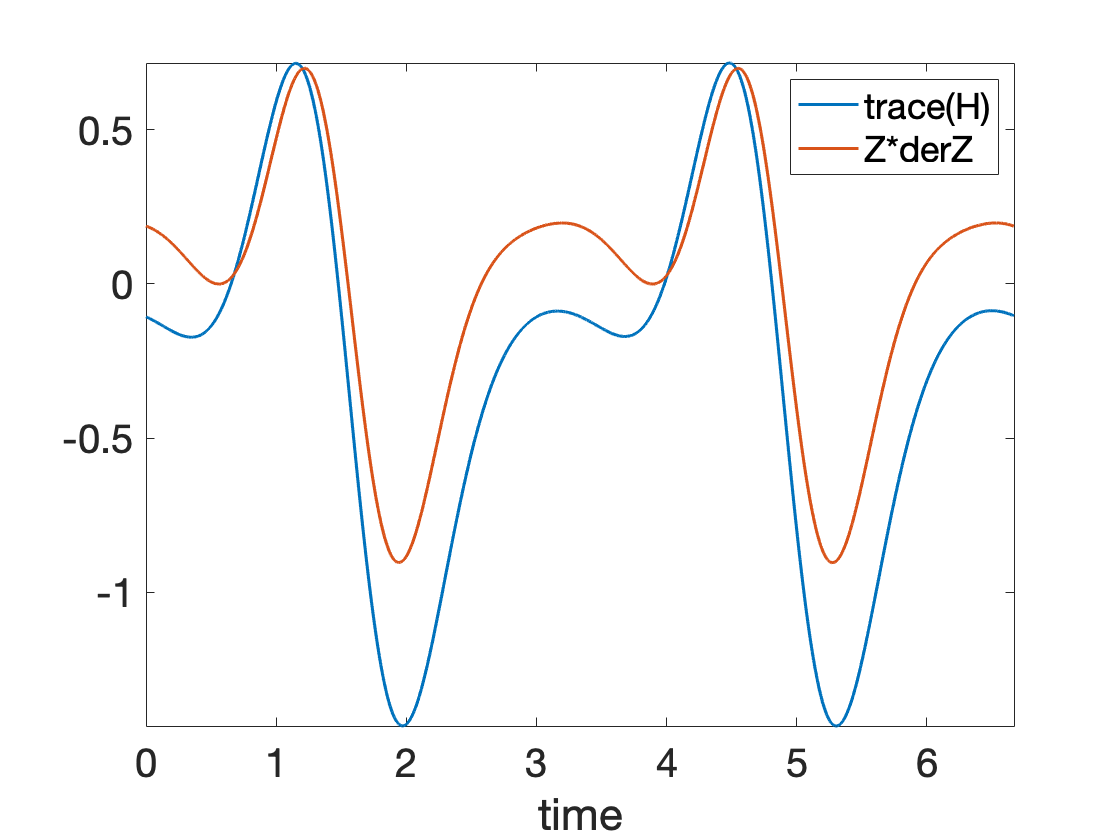
Figure 4: The comparison of $\boldsymbol{Z}(\theta)^{\top}\boldsymbol{Z}^{\prime}(\theta)$ and $\mathrm{tr}[\boldsymbol{H}(\theta)]$ in the Van der Pol oscillator.

References

• [1] A. T. Winfree, The Geometry of Biological Time, vol. 12. Springer Science & Business Media, 2001.
• [2] F. C. Hoppensteadt and E. M. Izhikevich, Weakly Connected Neural Networks, vol. 126. Springer Science & Business Media, 2012.
• [3] A. Demir, A. Mehrotra, and J. Roychowdhury, “Phase noise in oscillators: A unifying theory and numerical methods for characterization,” IEEE Transactions on Circuits and Systems—I: Fundamental Theory and Applications, vol. 47, no. 5, p. 655, 2000.
• [4] A. Hajimiri and T. H. Lee, “A general theory of phase noise in electrical oscillators,” IEEE Journal of Solid-State Circuits, vol. 33, no. 2, pp. 179–194, 1998.
• [5] A. Goldbeter, “Computational approaches to cellular rhythms,” Nature, vol. 420, no. 6912, p. 238, 2002.
• [6] G. B. Ermentrout and D. H. Terman, Mathematical Foundations of Neuroscience, vol. 35. Springer Science & Business Media, 2010.
• [7] Y. Kuramoto, Chemical Oscillations, Waves, and Turbulence. Courier Corporation, 2003.
• [8] T. Tateno and H. P. C. Robinson, “Phase resetting curves and oscillatory stability in interneurons of rat somatosensory cortex,” Biophysical journal, vol. 92, pp. 683–695, 2007.
• [9] N. W. Gouwens, H. Zeberg, K. Tsumoto, T. Tateno, K. Aihara, and H. P. C. Robinson, “Synchronization of firing in cortical fast-spiking interneurons at gamma frequencies: a phase-resetting analysis,” PLoS computational biology, vol. 6, p. e1000951, 2010.
• [10] M. A. Schwemmer and T. J. Lewis, “The theory of weakly coupled oscillators,” in Phase Response Curves in Neuroscience, pp. 3–31, Springer, 2012.
• [11] I. Malkin, Methods of Poincaré and Liapunov in the Theory of Nonlinear Oscillations. Moscow: Gostexizdat, 1949.
• [12] A. Winfree, “Patterns of phase compromise in biological cycles,” Journal of Mathematical Biology, vol. 1, no. 1, pp. 73–93, 1974.
• [13] J. Guckenheimer, “Isochrons and phaseless sets,” Journal of Mathematical Biology, vol. 1, no. 3, pp. 259–273, 1975.
• [14] N. W. Schultheiss, A. A. Prinz, and R. J. Butera, Phase Response Curves in Neuroscience: Theory, Experiment, and Analysis. Springer Science & Business Media, 2011.
• [15] P. Sacre and R. Sepulchre, “Sensitivity analysis of oscillator models in the space of phase-response curves: Oscillators as open systems,” IEEE Control Systems Magazine, vol. 34, no. 2, pp. 50–74, 2014.
• [16] E. Brown, J. Moehlis, and P. Holmes, “On the phase reduction and response dynamics of neural oscillator populations,” Neural Computation, vol. 16, no. 4, pp. 673–715, 2004.
• [17] J.-N. Teramae, H. Nakao, and G. B. Ermentrout, “Stochastic phase reduction for a general class of noisy limit cycle oscillators,” Physical Review Letters, vol. 102, no. 19, p. 194102, 2009.
• [18] J. T. C. Schwabedal and A. Pikovsky, “Effective phase dynamics of noise-induced oscillations in excitable systems,” Phys. Rev. E, vol. 81, p. 046218, Apr 2010.
• [19] J. T. C. Schwabedal and A. Pikovsky, “Phase description of stochastic oscillations,” Phys. Rev. Lett., vol. 110, p. 204102, May 2013.
• [20] J. M. Newby and M. A. Schwemmer, “Effects of moderate noise on a limit cycle oscillator: Counterrotation and bistability,” Phys. Rev. Lett., vol. 112, p. 114101, Mar 2014.
• [21] J. Moehlis, “Improving the precision of noisy oscillators,” Physica D: Nonlinear Phenomena, vol. 272, pp. 8–17, 2014.
• [22] P. J. Thomas and B. Lindner, “Asymptotic phase for stochastic oscillators,” Phys. Rev. Lett., vol. 113, p. 254101, Dec 2014.
• [23] M. Bonnin, “Phase oscillator model for noisy oscillators,” The European Physical Journal Special Topics, vol. 226, pp. 3227–3237, 2017.
• [24] M. Bonnin, “Amplitude and phase dynamics of noisy oscillators,” International Journal of Circuit Theory and Applications, vol. 45, no. 5, pp. 636–659, 2017.
• [25] P. C. Bressloff and J. N. MacLaurin, “A variational method for analyzing stochastic limit cycle oscillators,” SIAM Journal on Applied Dynamical Systems, vol. 17, no. 3, pp. 2205–2233, 2018.
• [26] P. J. Thomas and B. Lindner, “Phase descriptions of a multidimensional ornstein-uhlenbeck process,” Phys. Rev. E, vol. 99, p. 062221, Jun 2019.
• [27] P. C. Bressloff and J. N. MacLaurin, “Phase reduction of stochastic biochemical oscillators,” SIAM Journal on Applied Dynamical Systems, vol. 19, no. 1, pp. 151–180, 2020.
• [28] G. B. Ermentrout, B. Beverlin, T. Troyer, and T. I. Netoff, “The variance of phase-resetting curves,” Journal of Computational Neuroscience, vol. 31, pp. 185–197, 2011.
• [29] J.-N. Teramae and D. Tanaka, “Robustness of the noise-induced phase synchronization in a general class of limit cycle oscillators,” Physical Review Letters, vol. 93, no. 20, p. 204103, 2004.
• [30] X. Mao, Stochastic Differential Equations and Applications. Woodhead Publishing, second ed., 2011.
• [31] T. Menara, G. Baggio, D. S. Bassett, and F. Pasqualetti, “A framework to control functional connectivity in the human brain,” in 2019 IEEE 58th Conference on Decision and Control (CDC), pp. 4697–4704, 2019.
• [32] R. M. Ghigliazza and P. Holmes, “Minimal models of bursting neurons: How multiple currents, conductances, and timescales affect bifurcation diagrams,” SIAM Journal on Applied Dynamical Systems, vol. 3, no. 4, pp. 636–670, 2004.
• [33] R. M. Ghigliazza and P. Holmes, “A minimal model of a central pattern generator and motoneurons for insect locomotion,” SIAM Journal on Applied Dynamical Systems, vol. 3, no. 4, pp. 671–700, 2004.
• [34] E. Marder and D. Bucher, “Central pattern generators and the control of rhythmic movements,” Current Biol., vol. 11, no. 23, pp. R986–R996, 2001.
• [35] A. Ijspeert, “Central pattern generators for locomotion control in animals and robots: A review,” Neural Networks, vol. 21, no. 4, pp. 642–653, 2008.
• [36] Z. Aminzare, V. Srivastava, and P. Holmes, “Gait transitions in a phase oscillator model of an insect central pattern generator,” SIAM Journal on Applied Dynamical Systems, vol. 17, no. 1, pp. 626–671, 2018.
• [37] Z. Aminzare and P. Holmes, “Heterogeneous inputs to central pattern generators can shape insect gaits,” SIAM Journal on Applied Dynamical Systems, vol. 18, no. 2, pp. 1037–1059, 2019.
• [38] G. Russo, F. Wirth, and R. Shorten, “On synchronization in continuous-time networks of nonlinear nodes with state-dependent and degenerate noise diffusion,” IEEE Transactions on Automatic Control, vol. 64, no. 1, pp. 389–395, 2019.
• [39] G. Russo and R. Shorten, “On common noise-induced synchronization in complex networks with state-dependent noise diffusion processes,” Physica D: Nonlinear Phenomena, vol. 369, pp. 47–54, 2018.
• [40] A. M. Stanzhitskii, “Investigation of invariant sets of Itô stochastic systems with the use of lyapunov functions,” Ukrainian Mathematical Journal, vol. 53, pp. 323–327, 02 2001.
• [41] T. Björk, Arbitrage Theory in Continuous Time. Oxford University Press, 2009.
• [42] G. Giacomin, C. Poquet, and A. Shapira, “Small noise and long time phase diffusion in stochastic limit cycle oscillators,” Journal of Differential Equations, vol. 264, no. 2, pp. 1019–1049, 2018.
• [43] Z. Aminzare, P. Holmes, and V. Srivastava, “On phase reduction and time period of noisy oscillators,” in 2019 IEEE 58th Conference on Decision and Control (CDC), pp. 4717–4722, Dec 2019.
• [44] D. Wilson and B. Ermentrout, “Greater accuracy and broadened applicability of phase reduction using isostable coordinates,” Journal of Mathematical Biology, vol. 76, no. 1-2, pp. 37–66, 2018.
• [45] H. D. Macedo and J. N. Oliveira, “Typing linear algebra: A biproduct-oriented approach,” Science of Computer Programming, vol. 78, no. 11, pp. 2160–2191, 2013.
• [46] J. Guckenheimer and P. Holmes, Nonlinear oscillations, dynamical systems, and bifurcations of vector fields, vol. 42. Springer Science & Business Media, 2013.
• [47] M. Freidlin and A. Wentzell, Random Perturbations of Dynamical Systems. Springer-Verlag Berlin Heidelberg, third edition ed., 2012.