Causal Inference in the Time of Covid-19

Abstract

In this paper we develop statistical methods for causal inference in epidemics. Our focus is in estimating the effect of social mobility on deaths in the first year of the Covid-19 pandemic. We propose a marginal structural model motivated by a bbasic epidemic model. We estimate the counterfactual time series of deaths under interventions on mobility. We conduct several types of sensitivity analyses. We find that the data support the idea that reduced mobility causes reduced deaths, but the conclusion comes with caveats. There is evidence of sensitivity to model misspecification and unmeasured confounding which implies that the size of the causal effect needs to be interpreted with caution. While there is little doubt the effect is real, our work highlights the challenges in drawing causal inferences from pandemic data.

T1Ventura and Wasserman are members of the Delphi Group at CMU delphi.cmu.edu. This project arose from their work with Delphi. We are grateful for their help and support. We thank Rob Tibshirani and the reviewers for suggestions that greatly improved the paper. All the data can be obtained from the Delphi website covidcast.cmu.edu.

, and

August 10 2021

1 Introduction

During a pandemic, it is reasonable to expect that reduced social mobility will lead to fewer deaths. But how do we quantify this effect? In this paper we combine ideas from mechanistic epidemic models with modern causal inference tools to answer this question using state level data on deaths and mobility. Our goal is not to provide definitive estimates for the effects but rather to develop some methods and highlight the challenges in doing causal inference for pandemics. We also show how a generative epidemic model motivates a semiparametric causal model.

We use state death data at the weekly level. The data are available at the daily county level but the weekly state level data are more reliable. Indeed, the data are subject to many reporting issues. It is not uncommon for a state to fail to report many deaths for a few days and then suddenly report a bunch of unreported deaths on a single day. The problems are worse at the county level. Also, there are many small counties with very little data. We find using weekly state level data to be a good compromise between the quantity and quality of the data. We also note that epidemic analyses, such as flu surveillance, are generally done at the weekly level.

Epidemics are usually modeled by using generative models, which fully specify the distribution of the outcome (deaths). The most common epidemic models relate exposure, infections, recoveries and deaths by way of a set of differential equations. The simplest version is the SIR model (susceptible, infected, recovered) but there are many flavors of the model. We review the basic model in Section 4.

Instead of a generative model, we use a marginal structural model (MSM) (Robins, Hernan and Brumback (2000); Robins (2000)). An MSM is a semiparametric model that directly models the effect of mobility on death without specifying a generative model. Because it is semiparametric, it makes fewer assumptions than a generative model. However, our MSM is motivated by a modified SIR-type generative model.

We model deaths in each state separately to reduce confounding due to state differences. After obtaining model parameter estimates for each state, we will be interested in the causal question: what would happen if we set mobility to a certain value? For example, how many deaths would have occurred if mobility had been reduced earlier, or if people had remained more vigilant throughout? We follow standard causal language and refer to changing mobility as an intervention. A different notion of intervention would be a policy change like closing schools. In this case, mobility is a mediator meaning that the intervention affects the outcome through mobility. In this paper we focus on the effect of mobility on deaths and refer to hypothetically setting mobility to a certain value as an intervention. Providing estimates of the effect of mobility on deaths is valuable so that we can tell policy makers what mobility level they should aim for with their interventions. Analyzing the effect of interventions is also of interest but in this paper we focus on the effect of mobility on deaths.

We will see that the data provide evidence for an effect of mobility. But the data are very limited. As mentioned above, we use state-specific models with weekly resolution due to concerns about data quality and unmeasured confounding due to geographic differences. The result is that we have about 40 observations per state. With so little data, we are restricted to use fairly simple models. We do find significant causal effects but we conduct sensitivity analyses that show that the effects need to be interpreted cautiously. This sensitivity analysis includes assessing the impact of model assumptions and unobserved confounding.

Related Work. A number of researchers have considered modeling the effect of causal interventions (such as mobility and masks) on Covid-19. Notable examples are Unwin et al. (2020), Chang et al. (2020), and IHME (2020). These authors develop very detailed epidemic models of the dynamics of the disease. One advantage of such an approach is that one can then consider the effects of a large array of potential interventions. Further, the models themselves are of great interest for understanding the dynamics of Covid-19. However, these models are very complex, and they involve a large number of parameters including parameters for various latent variables. Fitting such models and assessing uncertainty is challenging. Some authors take a Bayesian approach with informative priors. Others use heuristics such as reporting intervals based on using various settings of the parameters. To the best of our knowledge, it is not known how to get valid, frequentist confidence intervals in these complex models. This is not meant as a criticism of these papers but rather, this reflects the intrinsic difficulty of dealing with such models. Furthermore, when used for causal analysis, parametrically specified epidemic models are susceptible to a problem known as the null paradox which we discuss in Section 4.2.

In contrast, our goal is to make the model as simple as possible and to use standard estimating equation methods so that standard errors can be obtained fairly easily. We do not claim that our approach is superior but we do believe that the model and the resulting confidence intervals are more transparent. Getting precise results from our simple model turns out to be challenging and raises doubts about the accuracy of published studies using highly complex models.

The papers by Chernozhukov, Kasahara and Schrimpf (2020) and Xiong et al. (2020) are much closer to ours. The authors of Chernozhukov, Kasahara and Schrimpf (2020) use a set of causal linear structural equations to model weekly cases as a function of social behavior (mobility) and social behavior as a function of policies. They model several policies simultaneously and they model all states simultaneously. They do obtain valid frequentist confidence intervals. Xiong et al. (2020) construct a measure of mobility inflow and using daily county level cases they fit a linear structural model to relate cases to mobility inflow. Our approach differs in several ways: we model deaths, we focus only on the effect of mobility, we model one state at a time, and we use a MSM rather than a generative model. By modeling within each state, we have much less data at our disposal, which makes modeling challenging. On the other hand, the threat of confounding due to state differences is reduced. By using a marginal structural model, our approach is semiparametric and so makes fewer assumptions. Unlike these authors, we focus on deaths instead of cases because we find the data on cases to be quite unreliable in general; for example, the availability of testing changed over time in various ways within and across states. Moreover, the data early in the pandemic are very important and this is when case data were least reliable. Also, we place a strong emphasis on sensitivity analysis. These analyses complement each other nicely.

Paper Outline. We describe the data in Section 2. In Section 3 we review some basics of causal inference. In Section 4 we construct the models that we will use and we explain how the models are fit in Section 5. The results are presented in Section 6. Concluding remarks are in Section 7.

2 Data

As mentioned earlier, we model each state separately, at the weekly level. The data for each state have the form

$$(A_{1},Y_{1}),\ldots,(A_{T},Y_{T})$$

where $A_{t}$ is mobility on week $t$ and $Y_{t}$ is the number of deaths due to Covid-19 on week $t$. We obtained our data from CMU’s Delphi group (cmu.covidcast.edu) which gets the death data from Johns Hopkins (https://coronavirus.jhu.edu) and the mobility data from Safegraph (safegraph.com). The data are from Feb 15 2020 (week 1) to December 25 2020 (week 45).

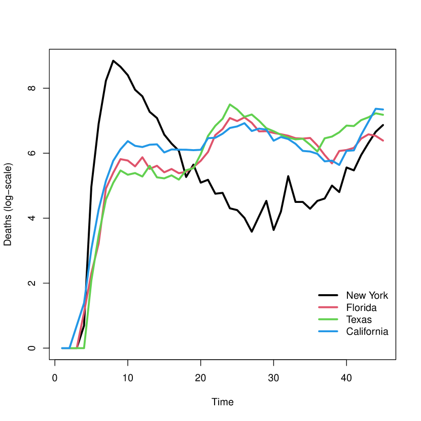
(a) Plot of log deaths versus time (weeks), from Feb 15 2020 (week 1) to December 25 2020 (week 45), for four populous states.

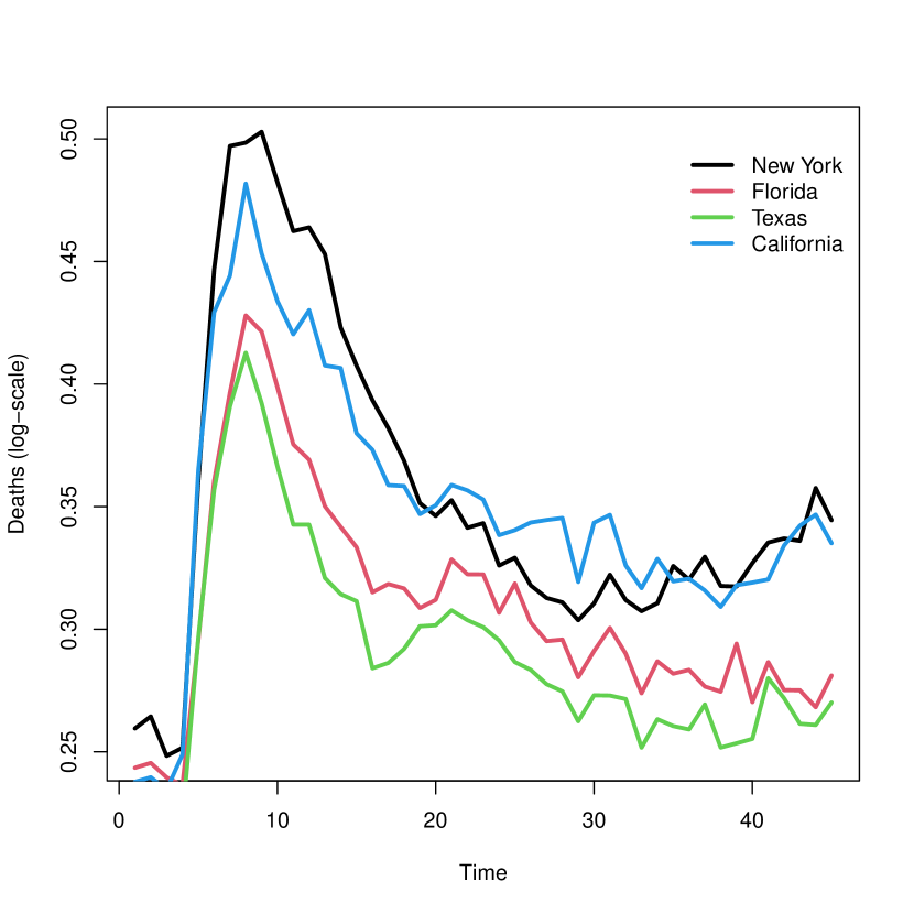
(b) Plot of anti-mobility measure “stay at home” versus week.

Figure 1: Plots of log deaths and anti-mobility across time.

Figure 1 shows log deaths $L_{t}=\log(Y_{t}+1)$ and “proportion at home” $A_{t}$ which is one of the mobility measures, for four states. This is the fraction of mobile devices that did not leave the immediate area of their home. In this case, a higher value means less mobility so we can think of this measure as anti-mobility. This is the variable we will use throughout. In the rest of the paper we standardize mobility by subtracting $A_{1}$ from each value of $A_{t}$ so that mobility starts at zero.

3 Causal Inference

In this section, we briefly review basic ideas from causal inference. Consider weekly mobility and death data $(A_{1},Y_{1}),\ldots,(A_{T},Y_{T})$ in one state. Define $\overline{A}_{t}=(A_{1},\ldots,A_{t})$ and $\overline{Y}_{t}=(Y_{1},\ldots,Y_{t})$ for $t\geq 1$.

Now consider the causal question: what would $Y_{t}$ be if we set $\overline{A}_{t}$ equal to some value $\overline{a}_{t}=(a_{1},\ldots,a_{t})$? Let $Y^{\overline{a}_{t}}_{t}$ denote this counterfactual quantity. It is important to distinguish the observed data $(\overline{A}_{T},\overline{Y}_{T})$ from the collection of unobserved counterfactual random variables

$$\Bigl{\{}Y^{\overline{a}_{T}}:\ \overline{a}_{T}\in\mathbb{R}^{T}\Bigr{\}},$$

which is an infinite collection of random vectors, one for each possible mobility trajectory $\overline{a}_{T}$. We make the usual consistency assumption that $\overline{Y}_{T}=\overline{Y}_{T}^{\overline{A}_{T}}$. To make sure this is clear, consider a simple case where a subject gets either treatment $A=1$ or control $A=0$. In this case, the random variables are $(A,Y,Y^{0},Y^{1})$ and the consistency assumption is that the observed outcome $Y$ satisfies $Y=Y^{1}$ if $A=1$ and $Y=Y^{0}$ if $A=0$.

Causal inference when the treatment varies over time is subtle. It may be tempting to simply regress $Y_{T}$ on the past and get the regression coefficient for mobility. This strategy has serious problems because $\overline{Y}_{T-1}$ are both confounding and mediating variables. Indeed, previous deaths can affect both future mobility and future deaths, while also being affected by previous mobility. More precisely, a large number of deaths implies a large number of infections which can cause future infections which then cause future deaths, and a large number of deaths might scare people into staying home. So we must adjust for past deaths. A common principle in epidemiology is to adjust for pre-treatment variables but not for post-treatment variables. But $Y_{s}$ comes after $A_{s-1}$ and before $A_{s+1}$ making it both a pre-treatment and post-treatment variable. So how do we properly define the causal effect?

The solution is to use Robins’ $g$-formula. Assuming for the moment that there are no other confounding variables except past deaths, Robins (1986) proved that the mean of $Y^{\overline{a}_{t}}_{t}$ is given by the g-formula:

$$\psi(\overline{a}_{t})\equiv\mathbb{E}[Y^{\overline{a}_{t}}_{t}]=\int\cdots\int\mathbb{E}[Y_{t}|\overline{A}_{t}=\overline{a}_{t},\overline{Y}_{t-1}=\overline{y}_{t-1}]\prod_{s=1}^{t-1}p(y_{s}|\overline{y}_{s-1},\overline{a}_{s})\ dy_{s};$$ (1)

$\psi(\overline{a}_{t})$ is the causal effect we seek to estimate. (We note that some authors denote $\mathbb{E}[Y^{\overline{a}_{t}}_{t}]$ by $\mathbb{E}[Y_{t}|{\rm do}(\overline{a}_{t})]$.) When there are other confounders $X_{t}$ besides past deaths, the formula becomes

$$\psi(\overline{a}_{t})\equiv\int\cdots\int\mathbb{E}[Y_{t}|\overline{A}_{t}=\overline{a}_{t},\overline{Y}_{t-1}=\overline{y}_{t-1},\overline{X}_{t-1}=\overline{x}_{t-1}]\prod_{s=1}^{t-1}p(y_{s},x_{s}|\overline{y}_{s-1},\overline{a}_{s},\overline{x}_{s-1})\ dy_{s}\,dx_{s}.$$

Intuitively, the $g$-formula can be obtained as follows. The density of $(\overline{y}_{t},\overline{a}_{t})$ can be written as

$$p(\overline{y}_{t},\overline{a}_{t})=\prod_{s=1}^{t}p(y_{s}|\overline{y}_{s-1},\overline{a}_{s})p(a_{s}|\overline{a}_{s-1},\overline{y}_{s-1}).$$ (2)

Now replace $p(a_{s}|\overline{a}_{s-1},\overline{y}_{s-1})$ with a point mass at $a_{s}$ (i.e. the $A$’s are fixed, no longer random) and then find of the mean of $Y_{t}$ from this new distribution. It will be useful later in the paper to bear in mind that $\psi(\overline{a}_{t})\equiv\psi(\overline{a}_{t},p)$ is a functional of the joint density $p$ from (2).

For the causal effect $\psi(\overline{a}_{t})$ to be identified we require three standard assumptions. These are: (1) there is no unmeasured confounding. Formally, this means that at each time, the treatment is independent of the counterfactuals given the past measured variables. (2) The distribution of treatment has a positive density. (3) Counterfactual consistency: If $\overline{A}_{t}=\overline{a_{t}}$ then $Y_{t}=Y^{\overline{a}_{t}}$. Later we add a fourth assumption, namely, that the dependence of mobility on the past satisfies a Markov condition.

The next question is: how do we estimate $\psi(\overline{a}_{t})$? A natural idea is to plug-in estimates of all the unknown quantities in the $g$-formula which leads to

$$\widehat{\psi}(\overline{a}_{t})\equiv\int\cdots\int\widehat{\mathbb{E}}[Y_{t}|\overline{A}_{t}=\overline{a}_{t},\overline{Y}_{t-1}=\overline{y}_{t-1}]\prod_{s=1}^{t-1}\widehat{p}(y_{s}|\overline{y}_{s-1},\overline{a}_{s})\ dy_{s}.$$ (3)

As discussed in Robins, Hernan and Brumback (2000); Robins (2000, 1989) there are a number of problems with this approach, called g-computation. If we plug-in nonparametric estimates, we quickly face the curse of dimensionality. If we use parametric estimates, we encounter the null-paradox (Robins and Wasserman (1997)): there may be no setting of the parameters which can represent the case where there is no treatment effect, i.e., there is no setting of the parameters which makes $\psi(\overline{a}_{t})$ a constant function of $\overline{a}_{t}$. We discuss the null paradox further in Section 4.2.

An alternative approach to estimating $\psi(\overline{a}_{t})$ (Robins, Hernan and Brumback (2000)) is to directly specify a parametric functional form $g(\overline{a}_{t},\beta)$ for $\psi(\overline{a}_{t})$. Such a model is called a marginal structural model (MSM). Robins, Hernan and Brumback (2000) showed that $\beta$ can be estimated by solving the following inverse-probability-weighted estimating equation:

$$\sum_{t}W_{t}^{*}\ h^{*}(\overline{A}_{t})(Y_{t}-g(\overline{A}_{t},\widehat{\beta}))=0,$$ (4)

where the weights $W_{t}^{*}$ are defined by

$$W_{t}^{*}=\prod_{s=1}^{t}\frac{1}{\pi(A_{s}|\overline{A}_{s-1},\overline{Y}_{s-1})}$$ (5)

and $\pi(a_{t}|\cdot)$ is the conditional density of mobility, assumed to be positive. We follow the common practice (Robins, Hernan and Brumback (2000)) of using stabilized weights

$$W_{t}=\prod_{s=1}^{t}\frac{\pi(A_{s}|\overline{A}_{s-1})}{\pi(A_{s}|\overline{A}_{s-1},\overline{Y}_{s-1})}.$$ (6)

which corresponds to setting $h^{*}(\overline{a}_{t})=h(\overline{a}_{t})\prod_{s=1}^{t}\pi(A_{s}\mid\overline{A}_{s-1})$ for some $h$. We discuss the choice of $h$ in Section 5. We will then find it convenient to rewrite (4) as

$$\sum_{t}W_{t}\ h(\overline{A}_{t})(Y_{t}-g(\overline{A}_{t},\widehat{\beta}))=0.$$ (7)

An MSM is a semiparametric model in the sense that it leaves the data generating process unspecified, subject to the restriction that the functional $\psi(\overline{a}_{t})$ has a specific form. Specifically, let us write $\psi(\overline{a}_{t})$ as $\psi(\overline{a}_{t},p)$ to make it clear that $\psi(\overline{a}_{t},p)$ depends on the joint density of the data $p(\overline{a}_{T},\overline{y}_{T})$ from (2). The model we are using is then

$${\cal P}=\Bigl{\{}p(\overline{a}_{T},\overline{y}_{T}):\ {\rm there\ exists\ }\beta\ {\rm such\ that\ }\psi(\overline{a}_{t},p)=g(\overline{a}_{t},\beta)\ {\rm for\ all\ }t\Bigr{\}}.$$ (8)

The model $g$ is typically chosen to be interpretable. For example, suppose that $g(\overline{a}_{t},\beta)=\beta_{0}+\beta_{1}\sum_{s}a_{s}$. Then the effect of the parameter settings is simple (i.e., mean outcomes only depend linearly on the amount of cumulative treatment), and the null (of no treatment effect) simply corresponds to $\beta_{1}=0$. It is important to keep in mind that this is not a model for the entire data generating process, just for marginal treatment effects, i.e., how mean outcomes under different treatment sequences are connected. Marginal structural models are often chosen to be some arbitrary but simple parametric model. Instead, we choose to specify the marginal structural model $g(a;\beta)$ by the following route: we tentatively specify a generative model and find a closed form formula $g(a,\beta)$ for $\psi(\overline{a}_{t})$. We then drop the generative model and use $g(a,\beta)$ as a MSM. We explain this in more detail in the next section.

Remark.

There is a difference between the standard MSM setup and the one we are considering that warrants mentioning. Typically one assumes access to $n$ different time series $(Z_{1},...,Z_{n}$), with each series $Z=\{(A_{1},Y_{1}),...,(A_{T},Y_{T})\}=(\overline{A}_{T},\overline{Y}_{T})$ observed for $n$ different independent units (e.g., states). There, one could have a different estimating equation at each time, for example,

$$\sum_{i}W_{ti}\ h_{t}(\overline{A}_{ti})(Y_{ti}-g_{t}(\overline{A}_{ti},\widehat{\beta}))=0$$

where the $i$ subscript denotes weights, treatments, outcomes, etc. for series $i$. If there are common parameters across timepoints, then these estimating equations could be combined, for example by summing over time, or using a generalized method of moments approach, etc. However, we model states individually, and so do not assume different states are independent. This leaves us with one observation per state at each time, which we then combine across time (but only within state) to obtain estimating equation (7). This represents the trade-off between independence versus modeling assumptions (e.g., Markov assumptions in the weights, or linearity in $g(\cdot)$): the less we require of one, the more we require of the other.

4 Models

Epidemics are often modeled using differential equations that describe the evolution of certain subgroups over time. Perhaps the most common is the SIR (Susceptible, Infected, Recovered) model (Kermack and McKendrick (1927), Brauer, Castillo-Chavez and Castillo-Chavez (2012), Bjørnstad (2018)) described by the equations

$$\frac{dS_{t}}{dt} =-\frac{\alpha I_{t}S_{t}}{N}$$

$$\frac{dI_{t}}{dt} =\frac{\alpha I_{t}S_{t}}{N}-\gamma I_{t}$$

$$\frac{dR_{t}}{dt} =\gamma I_{t},$$

where $N$ is population size, $S_{t}$ is the number of susceptibles, $I_{t}$ is the number of infected, $R_{t}$ are the removed (by death or recovery) at time $t$ and $\alpha>\gamma$. Solving the second equation conditional on $S_{t}$ yields $I_{t}=I_{t-1}e^{\int_{t-1}^{t}\alpha S_{t}/N-\gamma dt}$, which can be discretized as

$$I_{t}\approx I_{t-1}e^{\alpha S_{t}/N-\gamma}$$ (9)

when $S_{u}\approx S_{t}$ for all $u\in(t-1,t)$. Without intervention, the epidemic grows exponentially, peaks when $S_{t}/N=\gamma/\alpha$ and then decays exponentially. There are numerous generalizations of this model including stochastic versions, discretized versions and models with more states besides $S$, $I$ and $R$.

4.1 The Mobility Model

Our proposed MSM is

$$g(\overline{a}_{t},\nu_{0},\gimel,f)=\sum_{s=1}^{t}f(s,t)e^{\nu_{0}(s)+\sum_{r=1}^{s}\gimel(a_{r})}$$ (10)

with nuisance functions $f$, $\nu_{0}$ and $\gimel$. The model is motivated by the SIR model.

The basic idea of the SIR model is that there is a natural tendency for an epidemic to increase exponentially at the beginning. But there are also elements that reduce the epidemic such as the depletion of susceptible individuals due to recovery and death. At the beginning of a pandemic, reduction of susceptibles will play a negligible role. On the other hand, interventions like lockdowns, school closings etc can have a drastic effect. These considerations lead us to the following working model. We use this working model only to suggest a form for the MSM.

Let $I_{t}$ denote new infections in week $t$. Let

$$A_{t} \sim Q_{t}$$

$$I_{t} =I_{t-1}e^{c_{t}+\gimel(A_{t})}+\delta_{t}$$ (11)

$$Y_{t} =\sum_{s=1}^{t}f(s,t)I_{s}+\xi_{t}$$

where $Q_{t}$ is an arbitrary distribution depending on $(\overline{A}_{t-1},\overline{I}_{t-1},\overline{Y}_{t-1})$, $\delta_{t}$ and $\xi_{t}$ are mean 0 random variables (independent of the other variables), $f(s,t)$ denotes the probability that someone infected at time $s$ dies of COVID at time $t$, the parameter $c_{t}$ is a positive number and $\gimel$ is a smooth function. Notice that the infection process (second equation) has an exponential growth form as in (9), but we model the exponent directly as a function of mobility and time instead of stipulating a model for the susceptibles $S_{t}$. Here, $c_{t}$ represents the evolution of the epidemic without intervention and $\gimel(A_{t})$ is the effect of mobility. We allow $c_{t}$ to vary with $t$ to make the model more general and to allow the spread of Covid-19 to depend on the availability of susceptibles. We write

$$f(s,t)=d(s)f_{0}(s,t)$$ (12)

where $d(s)$ is the probability that someone infected at time $s$ will eventually die of COVID and $f_{0}(s,t)$ is the probability that someone infected at time $s$ and who will eventually die, will die at time $t$. Following Unwin et al. (2020) we take $f_{0}(s,t)$, on the scale of days, to be the density of $T_{1}+T_{2}$ where $T_{1}$ (time from infection to symptoms) is Gamma with mean 5.1 and coefficient of variation 0.86 and $T_{2}$ (time from symptoms to death) is Gamma with mean 18.8 and coefficient of variation 0.45. The resulting distribution can be accurately approximated by a Gamma with mean 23.9 days and coefficient of variation 0.40. Finally, we integrate this distribution over 7 day bins to get $f_{0}(s,t)$ on a weekly scale. A directed graph illustrating the model is given in Figure 2.

Figure 2: Directed graph illustrating the working model. Infections $I_{t}$ are unobserved. We use this model to find the form $g(a;\beta)$ of the causal effect $\psi(a)$. But when we estimate $\beta$ we use a semiparametric estimating equation approach; we do not fit the above model to the data.

At this point, we might use (4.1) as our model. But the $I_{t}$’s are not observed. Furthermore, a non-linear, sequentially specified parametric generative model can suffer from serious anomalies when used for causal inference. In particular, such a model can suffer from the null paradox (Robins (1986, 1989); Robins and Wasserman (1997)). This means that there may be no parameter values that satisfy (i) $Y_{t}$ is conditionally dependent on past values of $A_{s}$ and such that (ii) the null hypothesis of no treatment effect holds. We explain this point in more detail in Section 4.2.

Instead, we apply the $g$-formula to the model specified by (4.1) to find $\mbox{$\mathbb{E}$}[Y_{t}^{\overline{a}_{t}}]$ and use the resulting function as an MSM. This yields

$$\mbox{$\mathbb{E}$}[Y_{t}^{\overline{a}_{t}}]=\sum_{s=1}^{t}f(s,t)e^{\nu_{0}(s)+\sum_{r=1}^{s}\gimel(A_{r})}\equiv g(\overline{a}_{t},\nu_{0},\gimel,f)$$ (13)

where $\nu_{0}(s)=\log I_{1}+\sum_{r=1}^{s}c_{r}$. (We treat $I_{1}$ as an unknown parameter that is absorbed into $\nu_{0}$.) Now we abandon the working model and just interpret $g(\overline{a}_{t},\nu_{0},\gimel,f)$ directly as a model for the counterfactual $\mathbb{E}[Y^{\overline{a}_{t}}]$, that is, as an MSM. Put another way, we start with the model (4.1), find $g(\overline{a}_{t},\nu_{0},\gimel,f)=\mbox{$\mathbb{E}$}[Y^{\overline{a}_{t}}]$, and then expand the model to include all joint distributions that satisfy $\mbox{$\mathbb{E}$}[Y_{t}^{\overline{a}_{t}}]=g(\overline{a}_{t},\nu_{0},\gimel,f)$. This defines the model (8).

The MSM can be fit with the estimating equation (7), which corrects for confounding due to past deaths, not by modeling the entire conditional process, but by weighting by propensity weights $W_{t}$ given by (6). This MSM approach allows us to be agnostic about whether it is our motivating model (4.1) that holds, or some other much more complicated data-generating process. In fact, one can go further and take a completely agnostic view, in which the marginal structural model is not assumed correct at all, but only viewed as an approximation to the true, and possibly very complex, underlying counterfactual mean (Neugebauer and van der Laan, 2007).

To summarize, our approach involves three steps.

1. Tentatively specify a working model for infections $I_{t}$.

2. Find the resulting functional form $g(a;\beta)$ for $\psi(a)$ using the $g$-formula. We use $g(a;\beta)$ as our MSM.

3. Drop the working model and fit the MSM semiparametrically without further assumptions on the data generating process.

It is important to emphasize that when we estimate the causal parameter $\beta$, we do not assume any model for the epidemic process. Note that the model for $I_{t}$ in step 1 is very flexible but it does assume that the mobility effect is additive. An alternative would be to use a more sophisticated epidemic model for $\mbox{$\mathbb{E}$}[I_{t}|{\rm past}]$ in step 1. It would be interesting to do this and this would help unify the traditional approach to epidemic modeling with the MSM approach we are using. However, the implied function $g(a;\beta)$ would not be in closed form and it would be very hard to fit this model especially with only 40 observations.

4.2 The Null Paradox

To see how the null paradox works, consider a simple example with four time ordered variables $(A_{0},I_{1},A_{1},I_{2})$ where $A_{0}$ and $A_{1}$ are mobility and $I_{1}$ and $I_{2}$ are number of infected, which we assume are observed. This is a snippet of the entire time series. A simple epidemic model is

$$A_{0} \sim p(a_{0})$$

$$\log I_{1} =\beta_{0}+\epsilon$$

$$A_{1} \sim p(a_{1}|I_{1},A_{0})$$

$$\log I_{2} =\theta_{0}+\theta_{1}A_{0}+\theta_{2}\log I_{1}+\theta_{3}A_{1}+\delta$$

where $\epsilon$ and $\delta$ are, say, mean 0 Normal random variables. This is meant to capture exponential growth of $I_{t}$ (i.e. the SIR model at early times with no recovered individuals). By applying the $g$-formula, the causal effect of setting $A=(A_{0},A_{1})$ to $a=(a_{0},a_{1})$ is

$$\psi(a)=\mbox{$\mathbb{E}$}[\log I_{2}^{a}]=\theta_{0}+\theta_{1}a_{0}+\theta_{2}\beta_{0}+\theta_{3}a_{1}.$$

This means that, if we simulated the epidemic model with $A=(A_{0},A_{1})$ set to $a=(a_{0},a_{1})$, the mean of $\log I_{2}$ would precisely be $\theta_{0}+\theta_{1}a_{0}+\theta_{2}\beta_{0}+\theta_{3}a_{1}$. Suppose now that there is an unobserved variable $U$ that affects $I_{1}$ and $I_{2}$. For example, $U$ could represent the general health of the population. The variable $U$ is not a confounder as it does not affect $A_{0}$ or $A_{1}$. The causal effect is still given by the $g$-formula with no change. Suppose now that neither $A_{0}$ or $A_{1}$ have a causal effect on $I_{2}$. The set up is shown in Figure 3. Despite the fact that $A_{0}$ and $A_{1}$ have no causal effect on $I_{2}$, it may be verified that $I_{2}$ is conditionally dependent on $A_{0}$ and $A_{1}$. (This follows since $I_{1}$ is a collider on the path $I_{2},U,I_{1},A_{0},A_{1}$.) It follows that the maximum likelihood estimators $\widehat{\theta}_{1}$ and $\widehat{\theta}_{3}$ are not zero (and in fact converges to a nonzero number in the large sample limit). The estimated causal effect is

$$\widehat{\psi}(a)=\widehat{\theta}_{0}+\widehat{\theta}_{1}a_{0}+\widehat{\theta}_{2}\widehat{\beta}_{0}+\widehat{\theta}_{3}a_{1}$$

and will therefore be a function of $a$ even when $a$ has no causal effect.

The details of the model were not important. A similar model is

$$A_{0} \sim p(a_{0})$$

$$I_{1} \sim p(i_{1}|A_{0})$$

$$A_{1} \sim p(a_{1}|I_{1},A_{0})$$

$$I_{2} \sim p(i_{2}|A_{0},I_{1},A_{1})$$

where $\mbox{$\mathbb{E}$}[I_{2}|A_{0},I_{1},A_{1}]=e^{\beta_{0}+\beta_{1}A_{0}+\beta_{2}A_{1}}I_{1}$. In this case

$$\mbox{$\mathbb{E}$}[I_{2}^{a}]=e^{\beta_{0}+\beta_{1}a_{0}+\beta_{2}a_{1}}\mbox{$\mathbb{E}$}[I_{1}|A_{0}].$$

The same argument shows that the estimate will be a function of $a$ even when $a$ has no causal effect.

Figure 3: The null paradox. The directed graph is a snippet of the time series. Mobility is $(A_{0},A_{1})$ and number of infected individuals is $(I_{1},I_{2})$. The latent variable $U$ is not a confounder as it has no arrows to mobility. Neither $A_{0}$ nor $A_{1}$ have a causal effect on $I_{2}$. The variable $I_{1}$ is a collider, meaning that two arrowheads meet at $I_{1}$. This implies that $I_{2}$ and $(A_{0},A_{1})$ are dependent conditional on $I_{1}$. The estimate of the parameters that relate $I_{2}$ to $(A_{0},A_{1})$ in the epidemic model will be non-zero even though there is no causal effect.

4.3 Simplified Models

The MSM is not identified without further constraints. We will take $\gimel(A_{s})=\beta A_{s}$ so that

$$\mbox{$\mathbb{E}$}[Y_{t}^{\overline{a}_{t}}]=\sum_{s=1}^{t}f(s,t)e^{\beta\sum_{r=1}^{s}A_{r}+\nu_{0}(s)}.$$

Solving the estimating equation with this model is unstable and computationally prohibitive. Hence we make two approximations. First, we take $f_{0}(s,t)$ in (12) to be a point mass at $\delta=4$ weeks (approximately its mean). Then we get

$$\mbox{$\mathbb{E}$}[Y_{t}^{\overline{a}_{t}}]=e^{d(t-\delta)+\nu_{0}(t-\delta)+\beta M_{t}}$$

where $M_{t}\equiv M(\overline{a}_{t})=\sum_{s=1}^{t-\delta}a_{s}$. If we approximate $\log\mathbb{E}[Y_{t}^{\overline{a}_{t}}]$ with $\mathbb{E}[\log(Y_{t}^{\overline{a}_{t}})]$ we further obtain

$$\mathbb{E}[L_{t}^{\overline{a}_{t}}]=\log d(t-\delta)+\nu_{0}(t-\delta)+\beta M_{t}$$ (14)

where $L_{t}=\log(Y_{t}+1)$. Finally, we take

$$\nu(t)\equiv\log d(t-\delta)+\nu_{0}(t-\delta)=\sum_{j=1}^{k}\beta_{j}\psi_{j}(t)$$

where $\psi_{1},\ldots,\psi_{k}$ are orthogonal polynomials starting with $\psi_{1}(t)=t$. This model is easy to fit and will be used in Section 6. Note that the probability of dying $d(t)$ is allowed to change smoothly over time, which it likely did as hospitals were better prepared during the second wave. Interestingly, we have consistently found that using $k=1$ leads to unreasonable results as we discuss in Section which means that the disease exponential growth changes with time other than through mobility. The method for choosing $k$ is described in Section 6.2. Note that $\partial\mbox{$\mathbb{E}$}[L_{t}^{\overline{a}_{t}}]/\partial a_{s}=\beta$ for any $s\leq t-\delta$ so $\beta$ has a clear meaning.

The model in (14) was used independently in Shi and Ban (2020) with $k=1$. They used the model for curve fitting and they showed that this simple model fits the data surprisingly well. However, we find that making $\nu(t)$ non-linear (i.e. $k>1$) is important.

We will also consider a different approach to fitting the model. Specifically, we will use deconvolution methods to estimate the unobserved infection process $I_{1},\ldots,I_{T}$. The first equation in (4.1) implies $\mbox{$\mathbb{E}$}[I_{t}]=e^{\nu(t)+\beta\sum_{s}A_{s}}$ suggesting the MSM

$$\mbox{$\mathbb{E}$}[L_{t}^{\overline{a}_{t}}]=\nu(t)+\beta M_{t}$$

which is the same as (14) except that now $L_{t}=\log(I_{t})$ and $M_{t}=\sum_{s=1}^{t}a_{s}$ rather than $M_{t}=\sum_{s=1}^{t-\delta}a_{s}$.

Remark.

We have regularized the model by restricting $\nu(t)$ to have a finite basis expansion. We also considered a different approach in which $\nu(t)$ is restricted to be increasing which seems a natural restriction if $\nu(t)$ is supposed to represent the growth of the pandemic in lieu of intervention. (This is valid only at the start of the pandemic; later in the pandemic, $\nu$ could be decreasing.) Using the methods in Meyer et al. (2008, 2018); Liao and Meyer (2018) we obtained estimates and standard errors. The results were very similar to the results in Section 6.

Counterfactual Estimands. Now we discuss some causal quantities that we can estimate from the model. Let $\overline{a}_{t}=(a_{1},\ldots,a_{t})$ be a mobility profile of interest. After fitting the model we will plot estimates and confidence intervals for counterfactual deaths

$$\theta_{t}=\exp\Bigl{\{}\mbox{$\mathbb{E}$}[L^{\overline{a}_{t}}]\Bigr{\}}$$ (15)

under mobility regime $\overline{a}_{t}$, $t=1,\ldots,T$.

We will consider the following three interventions:

$${\rm Start\ one\ week\ earlier\ }:\ \overline{a}_{T}=(A_{2},A_{3},\ldots,,A_{T+1})$$

$${\rm Start\ two\ weeks\ earlier\ }:\ \overline{a}_{T}=(A_{3},A_{4},\ldots,A_{T+2})$$

$${\rm Stay\ vigilant\ }:\ \overline{a}_{T}=(A_{1},A_{2},\ldots,A_{9},A_{10},A_{10},A_{11},A_{11},A_{12},A_{12},A_{13},A_{13},\ldots)$$

The first two interventions aim to assess COVID-19 infections if we had started sheltering in place one and two weeks earlier. The last intervention halves the slope of the rapid decrease in stay at home mobility after the initial peak in week 9 that is clearly visible in Fig.1. See Figure 6.

5 Fitting the Model

Now we discuss the method for estimating the model.

5.1 Fitting the Semiparametric Model

Recall the MSM

$$\mathbb{E}[L_{t}^{\overline{a}_{t}}]=\nu(t)+\beta M(\overline{a}_{t})$$ (16)

where $\nu(t)=\sum_{j=1}^{k}\beta_{j}\psi_{j}(t)$. We estimate $\nu(t)$ and $\beta$ by solving the estimating equation

$$\sum_{t}h_{t}(\overline{a}_{t})W_{t}[L_{t}-(\widehat{\nu}(t)+\widehat{\beta}M(\overline{a}_{t}))]=0$$ (17)

corresponding to (7). We discuss the estimation of the weights $W_{t}$ in Section 5.2. As is often done for MSMs we choose

$$h_{t}(\overline{a}_{t})=(1,\psi_{1}(t),\ldots,\psi_{k}(t),M(\overline{a}_{t}))^{T}$$

since solving the estimating equation then corresponds to using least squares with weights $W_{t}$. The estimating equation is then the derivative of the weighted sum of squares set to zero.

Recall from (15) that $\theta_{t}=e^{\psi(\overline{a}_{t})}=e^{\nu(t)+\beta M(\overline{a}_{t})}$ which we estimate by $\widehat{\theta}_{t}=e^{\widehat{\nu}(t)+\widehat{\beta}M(\overline{a}_{t})}$. We obtain approximate confidence intervals using the delta method and the aymptotic normality of estimating equations estimators. The asymptotic variance is based on the heteroskedasticity and autocorrelation consistent HAC sandwich estimator (Newey).

5.2 Estimating the Stabilized Weights

To estimate the marginal structural model we need to estimate the stabilized weights

$$W_{t}=\prod_{s=1}^{t}\frac{\pi(A_{s}|\overline{A}_{s-1})}{\pi(A_{s}|\overline{A}_{s-1},\overline{Y}_{s-1})};$$

see (5) and (6). One approach is to plug in estimates of the numerator and denominator densities into the formula for $W_{t}$. But estimating these densities is not easy and ratios of density estimates can be unstable. The problem is exacerbated when we multiply densities. Instead we use a moment-based approach as in Fong et al. (2018); Zhou and Wodtke (2018). The idea is to estimate the vector of weights $W_{1},\ldots,W_{T}$ by noting that they need to satisfy certain moment constraints. Our method is similar to the approach in Zhou and Wodtke (2018).

We rewrite $W_{t}=\prod_{s=1}^{t}V_{s}$ where

$$V_{s}\equiv V_{s}(\overline{A}_{s},\overline{Y}_{s-1})=\frac{\pi(A_{s}|\overline{A}_{s-1})}{\pi(A_{s}|\overline{A}_{s-1},\overline{Y}_{s-1})}.$$

Let $\widetilde{h}_{1}(a_{t})$ and $\widetilde{h}_{2}(y_{t-1})$ be arbitrary functions and define their centered versions by

$$h_{1}(a_{t}) =\widetilde{h}_{1}(a_{t})-\mu_{t}$$

$$h_{2}(y_{t-1}) =\widetilde{h}_{2}(y_{t-1})-\nu_{t}$$

where the conditional means are

$$\mu_{t} \equiv\mu_{t}(\overline{A}_{t-1})=\mbox{$\mathbb{E}$}[\widetilde{h}_{1}(A_{t})|\overline{A}_{t-1}]$$

$$\nu_{t} \equiv\nu_{t}(\overline{A}_{t-\delta-1},\overline{Y}_{t-2})=\mbox{$\mathbb{E}$}[\widetilde{h}_{2}(Y_{t-1})|\overline{A}_{t-\delta-1},\overline{Y}_{t-2}].$$

Weighted products of these functions have mean zero since

$$\mbox{$\mathbb{E}$}[h_{1}(A_{t})h_{2}(Y_{t-1})W_{t}] =\int\cdots\int h_{1}(a_{t})h_{2}(y_{t-1})p(\overline{a}_{t},\overline{y}_{t-1})W_{t}(\overline{a}_{t},\overline{y}_{t-1})\,d\overline{a}_{t}\,d\overline{y}_{t-1}$$

$$=\int\cdots\int h_{1}(a_{t})h_{2}(y_{t-1})\pi(a_{t}|\overline{a}_{t-1},\overline{y}_{t-1})p(y_{t-1}|\overline{a}_{t-1},\overline{y}_{t-2})p(\overline{a}_{t-1},\overline{y}_{t-2})$$

$$\ \ \ \ \ \ \times\frac{\pi(a_{t}|\overline{a}_{t-1})}{\pi(a_{t}|\overline{a}_{t-1},\overline{y}_{t-1})}\left(\prod_{s=1}^{t-1}V_{s}\right)\ \ d\overline{a}_{t}\,d\overline{y}_{t-1}$$

$$=\int\Biggl{\{}\omega(\overline{y}_{t-2},\overline{a}_{t-1})\int h_{1}(a_{t})\pi(a_{t}|\overline{a}_{t-1})da_{t}\ \int h_{2}(y_{t-1})p(y_{t-1}|\overline{a}_{t-1},\overline{y}_{t-2})dy_{t-1}\Biggr{\}}d\overline{a}_{t-1}\,d\overline{y}_{t-2}$$

$$=0$$

from the definition of $h_{1}$ and $h_{2}$, where

$$\omega(\overline{y}_{t-2},\overline{a}_{t-1})=p(\overline{y}_{t-2},\overline{a}_{t-1})\prod_{s=1}^{t-1}V_{s}.$$

Thus, the weights are characterized by the moment constraints

$$\mbox{$\mathbb{E}$}[h_{1}(A_{t})h_{2}(Y_{t-1})W_{t}]=0.$$ (18)

As in Zhou and Wodtke (2018) we estimate the weights by finding $W_{t}$ to satisfy $\mbox{$\mathbb{E}$}[h_{1}(A_{t})h_{2}(Y_{t-1})W_{t}]=0$ for a set of functions $h_{1},h_{2}$. This requires estimating these moments and estimating $\mu_{t}$ and $\nu_{t}$. To proceed, we make a Markov assumption, namely

$$\mbox{$\mathbb{E}$}[\widetilde{h}_{1}(A_{t})|\overline{A}_{t-1}]=\mbox{$\mathbb{E}$}[\widetilde{h}_{1}(A_{t})|A_{t-1},\ldots,A_{t-k}]$$

and

$$\mbox{$\mathbb{E}$}[\widetilde{h}_{2}(Y_{t-1})|\overline{A}_{t-\delta-1},\overline{Y}_{t-2}]=\mbox{$\mathbb{E}$}[\widetilde{h}_{2}(Y_{t-1})|A_{t-1-\delta},\ldots,A_{t-k-\delta},{Y}_{t-2},\ldots,Y_{t-k}]$$

for some $k$. We will use $k=1$ in our analysis. Moreover, we assume homogeneity so that the functions $\mu_{t}$ and $\nu_{t}$ do not depend on $t$. Under the homogeneous Markov assumption, $\mu$ and $\nu$ can be estimated by regression. For example, if $k=1$, $\mu$ can be estimated by regressing $\widetilde{h}_{1}(A_{2}),\dots,\widetilde{h}_{1}(A_{T})$ on $A_{1},\ldots,A_{T-1}$. (We tried both linear and nonparametric regression and obtained similar weights from each approach so we have used linear regression in our results.) The sample versions of the moment conditions (18) are then

$$\frac{1}{T}\sum_{t}H_{tj}W_{t}=0$$

where

$$H_{tj}=(\widetilde{h}_{1j}(A_{t})-\widehat{\mu}_{j})(\widetilde{h}_{2j}(Y_{t-1})-\widehat{\nu}_{j})$$

and $\{(\widetilde{h}_{1j},\widetilde{h}_{2j}):\ j=1,\ldots,J\}$ are a set of pairs of functions, $\widehat{\mu}_{j}$ is the estimate of $\mbox{$\mathbb{E}$}[\widetilde{h}_{1}(A_{t})|A_{t-1},\ldots,A_{t-k}]$ and $\widehat{\nu}_{j}$ is the estimate of $\mbox{$\mathbb{E}$}[\widetilde{h}_{2}(Y_{t-1})|A_{t-1-\delta},\ldots,A_{t-k-\delta},{Y}_{t-2},\ldots,Y_{t-k}]$.

The moment conditions do not completely specify the weights. As in the above references we add a regularization term, in this case, $(1/2)\sum_{t}(W_{t}-1)^{2}$ and we require $\sum_{t}W_{t}=T$. This leads to the following minimization problem: minimize $W_{1},\ldots,W_{T}$ in

$$\frac{1}{2}\sum_{t}(1-W_{t})^{2}+\lambda_{0}\sum_{t}(W_{t}-T)+\sum_{j=1}^{J}\lambda_{j}\sum_{t}W_{t}H_{tj}$$ (19)

where the $\lambda_{j}$’s are Lagrange multipliers. The solution to the minimization is

$$W=\mathbf{1}-H(H^{T}H)^{-1}[H^{T}\bf{1}-D]$$ (20)

where $W=(W_{1},\ldots,W_{T})$, $\mathbf{1}$ is a vector of $1^{\prime}s$, $\mathbf{D}=(T,0,\ldots,0)^{T}$ and

$$H=\left(\begin{array}[]{cccc}1&H_{11}&\cdots&H_{1N}\\ 1&H_{21}&\cdots&H_{2N}\\ \vdots&\vdots&\vdots&\vdots\\ 1&H_{T1}&\cdots&H_{TN}\end{array}\right)$$

and $N$ is the total number of moment constraints. In our case we choose $h_{11}(a)=a$, $h_{12}(a)=a^{2}$, $h_{21}(y)=y$, $h_{22}(y)=y^{2}$.

To include other time varying confounders $X_{t}$ one should replace $h_{2}(y_{t-1})$ with two functions:

$$h_{2}(y_{t-1})=\widetilde{h}_{2}(y_{t-1})-\mbox{$\mathbb{E}$}[\widetilde{h}_{2}(y_{t-1})|\overline{X}_{t-1},\overline{A}_{t-1},\overline{Y}_{t-2}]$$

and

$$h_{3}(x_{t-1})=\widetilde{h}_{3}(x_{t-1})-\mbox{$\mathbb{E}$}[\widetilde{h}_{3}(x_{t-1})|\overline{X}_{t-2},\overline{A}_{t-1},\overline{Y}_{t-2}].$$

The steps for fitting the model are summarized in Fig.(4). Note that we cannot include past infections as a confounder since this variable is not observed. We choose not to include past cases or hospitalizations because the former is terribly biased downward at the beginning of the epidemic, and reliable data for the second is difficult to obtain. We need to assume that adjusting for past deaths serves as an adequate surrogate for infections, cases and hospitalizations. We address the more general problem of unoberved confounding in Section 6.2.

1. Choose the order $k$ of the Markov assumption. 2. Choose $J$ pairs of functions $\Bigl{\{}(\widetilde{h}_{1j}(a),\widetilde{h}_{1j}(y)):\ j=1,\ldots J\Bigl{\}}$. 3. Estimate $\mu_{j}=\mbox{$\mathbb{E}$}[\widetilde{h}_{1j}(A_{t})|A_{t-k},\ldots,A_{t-1}]$ and $\nu_{j}=\mbox{$\mathbb{E}$}[\widetilde{h}_{2j}(Y_{t-1})|A_{t-k-\delta-1},\ldots,A_{t-\delta-1},Y_{t-1-k},\ldots,Y_{t-2}]$ by regression. 4. Compute the weights $W_{1},\ldots,W_{n}$ from $(\ref{eq::W})$. 5. Fit the model $L_{t}=\beta\sum_{i=1}^{t-\delta}A_{s}+\nu(t)+\epsilon_{t}$ using weighed least squares with weights $W_{1},\ldots,W_{n}$.

Figure 4: Steps for fitting the model.

6 Results

In this section we give results for the mobility measure ‘proportion of people staying at home.’ We begin by showing the results of fitting the MSM to each state. Then we report on various types of sensitivity analysis.

6.1 Main Results

Figure 5(a) shows 95 percent confidence intervals for $\widehat{\beta}$ for each state from the marginal structural model in (16). We computed standard errors as if the weights were known, which results in valid but potentially conservative inference as long as the weight models are correctly specified (Tsiatis, 2007). The estimates are mostly negative, as would be expected, since higher $A_{s}$ means less mobility. Interestingly, we find that there turns out to be little confounding due to past deaths, as the fits with and without the estimated weights (not shown) are very similar. Nevertheless, we keep the weights in all the fits as a safeguard. In Section 6.2 we investigate this further by doing a sensitivity analysis.

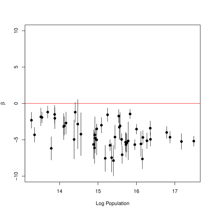
(a) Plot of $\widehat{\beta}$ and 95% confidence interval from the marginal structural model (16) for each state, versus state log population. A value of $\beta=-5$, for example, means that log deaths are reduced by 5 if $A_{s}$ is increased by one percent at any time $s$.

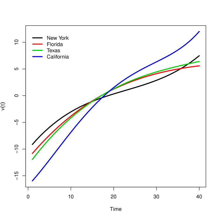
(b) Plot of $\widehat{\nu}(t)$ for four populous states.

Figure 5: Estimates of the MSM parameters defined in (16).

Figure 5(b) shows the estimated smooth function $\widehat{\nu}(t)$ in (16) for four states. The functions are increasing with slopes tapering off as time goes by, and picking back up again in NY and CA around week 35, consistent with deaths rising at that time in these two states; see Figure 1. The shape of $\widehat{\nu}(t)$ is consistent with the usual epidemic dynamics where it is assumed that this component should initially grow (linearly with no interventions and with an infinite pool of susceptibles) on the log-scale at the start of the epidemic and then decrease. Some of the non-linearity probably reflects the fact that the probability $d(t)$ of dying decreases over time due to better hospital treatment, social distancing changes, and the number of susceptibles to COVID-19 decreases over time as recovered patients are likely immune for some period post-infection.

Next we consider counterfactual deaths $\theta_{t}=\exp(\mbox{$\mathbb{E}$}[L^{\overline{a}_{T}}])$ in (15) for the three mobility scenarios described at the end of section 4; two mobility scenarios are shown in Figure 6 for four states. Figure 7 shows the estimates and pointwise 95 percent confidence bands for $\theta_{t}$ for these four states. The plots for all states are in the Supplement.

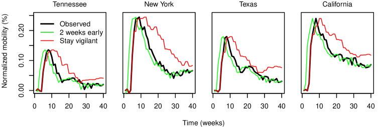
Figure 6: The observed mobility curves and hypothetical interventions for four states. Mobility has been standardized to have value 0 at the beginning of the series. All plots are on the same scale.

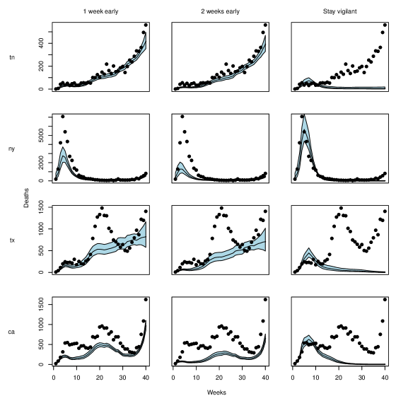
Figure 7: Pointwise 95% confidence bands for deaths $\theta_{t}=\exp(\mbox{$\mathbb{E}$}[L^{\overline{a}_{T}}])$ for the three mobility scenarios $\overline{a}_{T}$ described at the end of section 4; see also Figure 6. Each row is a different state. Each column is a different scenario, start one week early, start two weeks early and stay vigilant. The epidemic in NY started early so staying at home sooner had a large impact. The same is true for PA, IL, MI, NJ, MA. Staying home earlier would not have had as much impact in states such as TN that did not suffer the epidemic early. Staying more vigilant would have had a large impact except for New York. Some lack of fit in the early time period is evident in Texas, where counterfactual deaths exceed observed deaths under ‘stay vigilant’ where mobility has not yet been changed.

Finally, Figure 8 shows 95 percent confidence intervals for $\sum_{t}\exp\left(\mathbb{E}[L^{\overline{a}_{t}}]\right)-\sum_{t}Y_{t}$ and for $\left(\sum_{t}\exp\left(\mathbb{E}[L^{\overline{a}_{t}}]\right)-\sum_{t}Y_{t}\right)/\sum_{t}Y_{t}$ under the ‘stay vigilant’ scenario. We refer to these as total and relative excess deaths, where a negative excess means that lives would be saved. Of course, this number is larger for more populous states, although relative to the total number of observed deaths, all states small and large would have benefited equally from more sustained vigilance. Note that the confidence interval for New York (fourth from right) is very large. New York experienced the pandemic early and responded with large values of $A_{s}$ so it is believable that further vigilance may not have a large effect.

Figure 8: 95% confidence intervals for total excess deaths $\sum_{t}\exp\left(\mathbb{E}[L^{\overline{a}_{t}}]\right)-\sum_{t}Y_{t}$ (top) and relative excess deaths $\left(\sum_{t}\exp\left(\mathbb{E}[L^{\overline{a}_{t}}]\right)-\sum_{t}Y_{t}\right)/\sum_{t}Y_{t}$ (bottom) under the ‘stay vigilant’ scenario. The confidence intervals for NY (fourth from right) and a handful of other states include zero and suggests that staying more vigilant would not have significantly impacted the death toll. On the other hand, many states, small and large, could have reduced their death tolls by over a half.

We now compare our results to those in Unwin et al. (2020). They use a sophisticated model of the epidemic dynamics so a direct comparison is difficult. They estimate a parameter $R_{t}$ that measures how many individuals an infected person will infect. Using a Bayesian approach, they find a 95 percent posterior interval for the change in $R_{t}$ for the U.S. when setting mobility to its maximum value is [26.5,77.0]. The log of the change in $R_{t}$ is roughly equivalent to $-\beta$ in our setting. On the log scale, their interval is [3.3,4.3]. Our effect sizes are similar and slightly larger for the large states. For the middle sized states our effect estimates vary somewhat and are sometimes larger and sometimes smaller than theirs. Overall, the effect estimates are quite similar which is reassuring given how vastly different the methods are. Another point of comparison is Chernozhukov, Kasahara and Schrimpf (2020) who consider a very ambitious model which includes multiple policy interventions and multiple mobility measures (which they call behavior) simultaneously and the model is over all states. Their estimate of the mobility effect on log cases is -0.54 with a standard error of .19. Unlike Unwin et al. (2020), this estimate is very different from ours. We do not know why the effect size is so different from ours. They are using a different measure of mobility (they used Google mobility) which might have some effect. It is possible that some of the mobility effect might be absorbed into their policy effect which could happen if there is model misspecification.

6.2 Sensitivity Analysis

We have made a number of strong assumptions in our model. Our preference would be to weaken these assumptions and use nonparametric methods but the data are too limited to do so. Instead, we now assess the sensitivity of the results to various assumptions. We consider various perturbations of our analysis. These include: (1) changing the model/estimation method (we replace the MSM with a generative model), (2) assessing the Markov assumption (which was used to estimate the weights), (3) checking the accuracy of the point mass approximation (which was used in Section 4.3 to simplify the model) and (4) assessing sensitivity to unmeasured confounding (we have assumed that the only time varying confounders are past values of mobility and death).

1. An Alternative Model. Here we compare the results from the MSM in (16) to the time series AR(1) model:

$$L_{t}=L_{t-1}+\beta A_{t-\delta}+r(t)+\epsilon_{t}$$ (21)

where $r(t)$ is a polynomial of degree $k-1$. This says that, apart from random error, $L_{t}$ differs from $L_{t-1}$ for two reasons, mobility $A_{t-\delta}$ and the natural increase $r(t)$ due to epidemic dynamics (at the start of the epidemic). If we apply the $g$-formula in (1) to this model, we find $\mbox{$\mathbb{E}$}[L_{t}^{\overline{a}_{t}}]=\beta M(\overline{a}_{t})+\nu(t)$ where $\nu(t)=\sum_{s=1}^{t}r(s)$ is a polynomial of order $k$. Hence, this model is consistent with the MSM. In other words, this model is contained in the semiparametric model ${\cal P}$ defined in (8). This model resembles Robins’ blip models (Robins (2000); Vansteelandt et al. (2014)) as it measures the effect of one blip of treatment $A_{t-\delta}$ so we will refer to (21) as the blip model. We will fit (21) by least squares. There are three reasons for fitting this model. First, it as a point of comparison for the MSM. Second, we are able to check residuals and model fit. Third, since it is a regression model, we can use AIC to choose the degree $k-1$ of $r(t)$. We also use this choice of $k$ in the MSM. The degree $k$ chosen by AIC is typically $k=1$ for small states and $k=3$ or $k=4$ for the larger states. A plot of the selected degree versus log population and versus log deaths is in the supplementary material.

The left plot in Figure 9 shows the estimates of $\beta$ and 95 percent confidence intervals for all the states from the blip model in (21), and the right plot compares the estimates of $\beta$ from the MSM and blip models, where we see the similarity of the inferences. Since the blip model is a regression model, it makes sense to compare the observed data to the fits. Fig 10 shows the fitted values and the data for four states. The fit is not perfect but is reasonable. There are some large outliers in some states, mostly in the first few weeks of the pandemic where mobility $A_{t}$ and log deaths $L_{t}$ change rapidly. Because of this we also fitted a robust regression but the results did not change much.

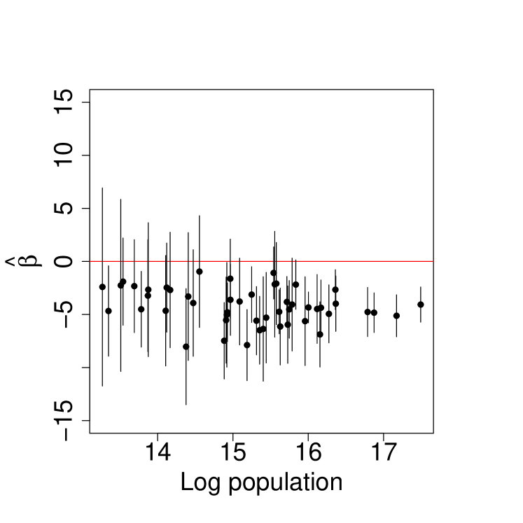
(a) Estimates of $\beta$ from the blip model in
(21) with 95% confidence intervals.

(b) Comparison of estimates of $\beta$ from the blip model and the MSM in (16).

Figure 9: Estimates from the blip model compared with estimates from the MSM model.

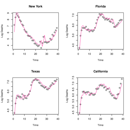
Figure 10: Observed log deaths in four states as functions of time with estimates (red) from the blip model in (21).

2. The Markov Assumption. In Section 5.2, to estimate the weights, we have made the Markov assumption that $A_{t-\delta}$ is conditionally independent of the past given $(A_{t-1-\delta},L_{t-1-\delta})$. We also assumed that $L_{t}$ is conditionally independent of the past given $(A_{t-1-\delta},L_{t-1})$. To assess this assumption, we fit the models

$$A_{t-\delta} =\alpha_{0}+\alpha_{1}A_{t-1-\delta}+\alpha_{2}A_{t-2-\delta}+\alpha_{3}A_{t-3-\delta}+\beta_{1}L_{t-1-\delta}+\beta_{2}L_{t-2-\delta}+\beta_{3}L_{t-3-\delta}+\epsilon_{t}$$

$$L_{t} =\alpha_{0}+\alpha_{1}A_{t-\delta}+\alpha_{2}A_{t-\delta-1}+\alpha_{3}A_{t-\delta-2}+\beta_{1}L_{t-1}+\beta_{2}L_{t-2}+\beta_{3}L_{t-3}+\delta_{t}.$$

Figure 11 shows boxplots of the t-statistics for these parameters. The evidence suggests that the first order Markov assumption is reasonable. The weak dependence of $A_{t}$ on past values of $Y_{t}$ is consistent with the weights $W_{t}$ having almost no effect, i.e. there is little confounding due to past deaths. However, this assessment still assumes that the Markov assumption is homogeneous, that is, that the law of $A_{t}$ given $(A_{t-1},Y_{t-1})$ is constant over time. This assumption is not checkable without invoking further assumptions.

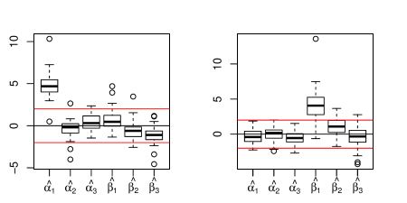
Figure 11: (Left) Boxplots across states of $t$-statistics for the parameters in the model for $A_{t}$ as a function of the past. The horizontal red lines are at $\pm 2$. Only $\widehat{\alpha}_{1}$ is consistently significantly different from zero across states, suggesting that the times series of at home mobility $A_{t}$ is a memory one process. (Right) Same for $Y_{t}$. Only $\widehat{\beta}_{1}$ is consistently significantly different from zero across states, suggesting that the deaths times series $Y_{t}$ is a memory one process.

3. Point Mass Versus Deconvolution. Recall that in Section 4.3 we approximated $f_{0}(s,t)$ with a point mass at $t-\delta$ with $\delta=4$. An alternative is to solve the estimating equation using $g$ defined as in (10) but this is numerically very unstable. Yet another alternative to the point mass approximation is to estimate the number of infections $I$ by deconvolution. From the number of infections, we can estimate the model parameters as in Section 5 without making the point mass approximation, using $\log(I)$ as the outcome variable. We infer $\widetilde{I}_{t}=d(t)I_{t}$ from the optimization:

$$\min_{I\geq 0}\|Y-F\widetilde{I}\|_{2}^{2}+\lambda\sum_{r=2}^{T-1}(\widetilde{I}_{r}-\widetilde{I}_{r-1})^{2},$$ (22)

where $Y$ denotes the vector of weekly deaths and $F$ is a matrix with $(i,j)$-entry equal to $f(i,j)$ if $j\leq i$ and zero otherwise; that is, $F_{ij}$ is proportional to the probability of dying at time $j$ given that infection occurred at time $i$. The parameter $\lambda$ is user-specified and represents a penalty imposed on non-smooth solutions. Because $f$ is proportional to the density of a Gamma random variable, we have $F_{ii}=f(i,i)=0$. To ensure nonzero elements on the diagonal of $F$, we remove the first row and last column (all zeros) from $F$ and solve (22) using $Y=(Y_{2},\ldots,Y_{T})$, thus obtaining an estimate of $\widetilde{I}=(\widetilde{I}_{1},\ldots,\widetilde{I}_{T-1})$. To enforce nonnegative values of $I$, we use the constrained optimization routine L-BFGS-B from optim in R. Using a penalty $\lambda=1$, we report the inferred infections (up to proportionality) $\widehat{I}$ (red line) for California, Florida, New York and Texas in Figure 13 along with the implied deaths computed as $F\widehat{I}$. The latter match the observed deaths well, leading credence to this procedure. In Figure 13, we compare the estimates of $\beta$ from the MSM using the point-mass approximation and those from the MSM using the estimates of infections from the deconvolution step. The estimates are in rough agreement as they lie near the diagonal.

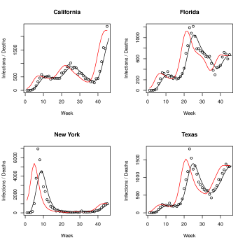
Figure 12: Inferred infections in four states. The red curve is $\widehat{\widetilde{I}_{t}}$, the estimate of the number of infections times the probability of dying if infected by Covid-19, $\widetilde{I}_{t}=d(t)I_{t}$. The black curve is deaths $F\widehat{I}$ computed from the optimization with $\lambda=1$ in (22), and the dots are the observed deaths.

Figure 13: Comparison of estimates of $\widehat{\beta}$ from the MSM using the point-mass approximation versus using estimates of infections via deconvolution for different values of $\lambda$.

4. Unmeasured Confounding. At time $t$, we treated $(A_{1},Y_{1}),\ldots,(A_{t-1},Y_{t-1})$ as confounders. Now suppose there is an unmeasured confounder $U$. We would like to assess $|\widehat{\beta}_{U}-\widehat{\beta}|$ where $\widehat{\beta}_{U}$ is the value of our estimate if we had access to $U$. This quantity is not identified and so any sensitivity analysis must invoke some extra assumption. Let $\Delta=|\widehat{\beta}_{U}-\widehat{\beta}|/{\rm se}(\widehat{\beta})$ denote the unobserved confounding on the standard error scale. So $\Delta=0$ corresponds to no unmeasured confounding, $\Delta=1$ corresponds to saying that the unmeasured confounding is the same size as the standard error, etc. For each state, we enlarge the confidence interval by $\Delta\,{\rm se}(\widehat{\beta})$. We can then ask: how large would $\Delta$ have to be so that the enlarged confidence interval would contain 0. Figure 14(a) shows this critical $\Delta$. We see that for most states, it takes a fairly large $\Delta$ to lose statistical significance. A substantial number of medium to large states are are quite robust to unmeasured confounding.

Adding other potential within state confounders would be desirable but, in a within-state analysis, we can only accommodate time varying confounders. (A fixed confounder is a single variable with no replication and can only be used an across state analysis.) So far we do not have any within-state time varying variables that would be expected to directly affect both $A_{t}$ and $Y_{t}$. One could imagine that a variable like “the percentage of rural cases” could change over time and possibly affect both variables but we do not have such data.

(a) Minimum value of $\Delta$ versus log-population for each state, such that unmeasured confounding of size $\Delta\,{\rm se}(\widehat{\beta})$ causes the confidence interval for $\beta$ to contain 0. For most states, it takes a fairly large $\Delta$ to lose statistical significance.

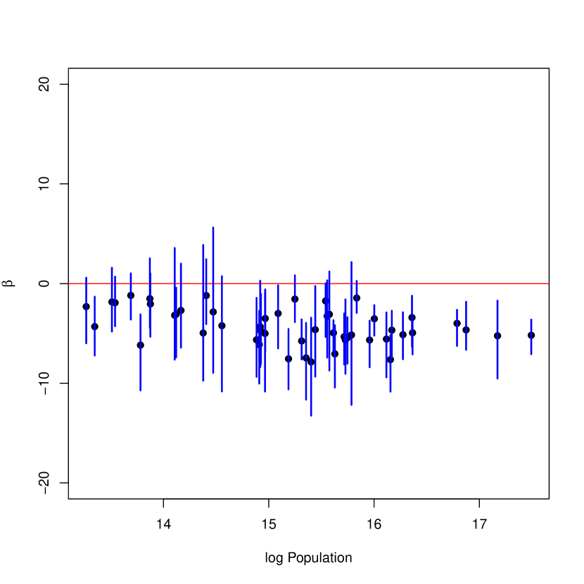
(b) The blue line segments span the lower and upper bounds of $\widehat{\beta}$ over the weights $1/\Gamma\leq\widetilde{W}_{t}/W_{t}\leq\Gamma$ with $\Gamma=3$. The black dots are the original point estimates. The effects for most large and medium states remain significant, indicating robustness to unmeasured confounding.

Figure 14: Unmeasured confounding sensitivity plots.

Next we consider a second style of sensitivity analysis inspired by the approach in Rosenbaum et al. (2010). The effect of unmeasured confounding in our analysis is that the weights $W_{t}$ are misspecified. If there are unobserved confounders $U_{t}$, then the correct weights are

$$\widetilde{W}_{t}=\prod_{s=1}^{t}\frac{\pi(A_{s}|\overline{A}_{s-1})}{\pi(A_{s}|\overline{A}_{s-1},\overline{Y}_{s-1},\overline{U}_{s-1})}$$

whereas we estimated the weights

$$W_{t}=\prod_{s=1}^{t}\frac{\pi(A_{s}|\overline{A}_{s-1})}{\pi(A_{s}|\overline{A}_{s-1},\overline{Y}_{s-1})}.$$

To assess this impact we find the maximum and minimum $\widehat{\beta}$ under the assumption that

$$\frac{W_{t}}{\Gamma}\leq\widetilde{W}_{t}\leq\Gamma W_{t}$$

for $t=1,\ldots,T$ and some $\Gamma\geq 1$. Similar ideas for static, binary treatments have been considered in Zhao, Small and Bhattacharya (2019); Yadlowsky et al. (2018). Figure 14(b) shows the bounds on $\widehat{\beta}$ using $\Gamma=3$. Even with this fairly large value of $\Gamma$ the effects for most large and medium states remain significant indicating robustness to unmeasured confounding. (The method for computing the bounds is in Bonvini et al. (2021).)

6.3 Across Versus Within States

We have focused on within state estimation. An alternative is to fit a model across states as well. Although we are skeptical of combining data over states we do so here for completeness. We fit the blip model with common $\beta$ and, rather than include state level covariates such as population size, proportion of residents in cities, etc., we use a fixed effect for each state. The resulting estimates of $\beta$ and standard errors for $k=1,2,3,4$ are:

$k$	$\widehat{\beta}$	standard error
1	-5.20	0.27
2	-4.60	0.27
3	-3.82	0.34
4	-2.83	0.43

The estimates are consistent with the within state models. AIC chooses $k=1$, which conflicts with the within state analysis with favors larger $k$ for larger states. The likely reason is that combining states adds variability in the combined dataset since $\beta$’s and $\nu(t)$’s are different between states, so there is less signal compared to the noise to estimate a more complicated relationship than a linear. A natural extension of this model is to use a random effects approach, although we do not pursue that here.

7 Discussion

Our approach to modeling the causal effect of mobility on deaths is to construct a marginal structural model whose parameters are estimated by solving an estimating equation. We model each state separately to reduce confounding due to state differences. Our approach has several advantages and disadvantages.

Our modeling assumptions are reasonable in the short term but not in the long term. Eventually, the effects of acquired immunity, masks, vaccinations etc might have to be accounted for by using a more complex form of $\nu$. Also, the effect of mobility $\beta$ could change with new variants.

Estimating the model parameters comes down to solving the estimating equation (17). Computing standard errors and confidence intervals is then straightforward. This is in contrast to more traditional and Icarian epidemic modeling which requires estimating many parameters using grid searches or MCMC. Provably valid confidence intervals are elusive for those methods. On the other hand, the more detailed models might be more realistic and can capture effects that our simple model cannot capture. Moreover, our inferences are asymptotic in nature. When comparing exact Bayesian methods to approximate frequentist methods it is hard to argue that one approach is more valid than the other.

We believe that focusing on weekly data at the state level gives us the best chance of getting data of reasonable quality and helps avoid confounding related to state differences. Further, this allows the causal effect to vary between states. But this results in a paucity of data, a few dozen observations per state. This limits the complexity of the models we can fit and it requires that we make a homogeneous Markov assumption. A natural compromise worthy of future investigation would be to use some sort of random effects model to allow modeling all states simultaneously. This could also permit using data from other countries. At any rate, there is a tradeoff: within state analysis requires stronger modeling assumptions while analyzing all states together requires assuming independence and it assumes we can model all sources of between state confounding.

Detailed dynamic modeling versus the more traditional causal modeling done here (and in Chernozhukov, Kasahara and Schrimpf (2020)) represent two different approaches to causal inference for epidemics. It would be interesting to see a general comparison of these approaches, perhaps eventually leading to some sort of fusion of these ideas.

Finally, let us recap the null paradox. Any nonlinear, sequentially specified parametric model — which includes most epidemic models — has the following problem. There is no value of the parameters that allows both (i) the outcome is conditionally dependent on the intervention variable $A$ and (ii) there is no causal effect of $A$. But, due to baseline variables $U$, (i) and (ii) can both be true. This means that we would find a causal effect even if there is no such effect. We can in principle avoid the null paradox by using nonparametric models but then the model complexity explodes as $T$ increases leading to the curse of dimensionality. Linear models avoid the null paradox but caution is still needed since the causal effect $\psi(a)$ involves complicated nonlinear functions of the regression parameters. Hence, the model is very difficult to interpret and the individual regression parameters do not have a causal interpretation. Also, most epidemic models are not linear.

The quickly growing literature on using sequentially specified epidemic models does include such models. MSMs avoid the null paradox, and this is another reason for using MSMs (or some other semiparametric causal model such as structural nested models). In our case we motivated the MSM by starting with a sequentially specified model. This seems like a reasonable approach for using epidemic models to define an MSM but there may be other approaches as well.

References

- Bjørnstad (2018) {barticle}[author] \bauthor\bsnmBjørnstad, \bfnmOttar N\binitsO. N. (\byear2018). \btitleEpidemics. \bjournalModels and data using R: Springer International Publishing \bpages318. \endbibitem
- Bonvini et al. (2021) {barticle}[author] \bauthor\bsnmBonvini, \bfnmM.\binitsM., \bauthor\bsnmKennedy, \bfnmE.\binitsE., \bauthor\bsnmVentura, \bfnmV.\binitsV. and \bauthor\bsnmWasserman, \bfnmL.\binitsL. (\byear2021). \btitlePropensity Scores and Sensivity Analysis for Marginal Structural Models with Continuous Treatments. \bjournalIn preparation. \endbibitem
- Brauer, Castillo-Chavez and Castillo-Chavez (2012) {bbook}[author] \bauthor\bsnmBrauer, \bfnmFred\binitsF., \bauthor\bsnmCastillo-Chavez, \bfnmCarlos\binitsC. and \bauthor\bsnmCastillo-Chavez, \bfnmCarlos\binitsC. (\byear2012). \btitleMathematical models in population biology and epidemiology \bvolume2. \bpublisherSpringer. \endbibitem
- Chang et al. (2020) {barticle}[author] \bauthor\bsnmChang, \bfnmSerina\binitsS., \bauthor\bsnmPierson, \bfnmEmma\binitsE., \bauthor\bsnmKoh, \bfnmPang Wei\binitsP. W., \bauthor\bsnmGerardin, \bfnmJaline\binitsJ., \bauthor\bsnmRedbird, \bfnmBeth\binitsB., \bauthor\bsnmGrusky, \bfnmDavid\binitsD. and \bauthor\bsnmLeskovec, \bfnmJure\binitsJ. (\byear2020). \btitleMobility network models of COVID-19 explain inequities and inform reopening. \bjournalNature \bpages1–6. \endbibitem
- Chernozhukov, Kasahara and Schrimpf (2020) {barticle}[author] \bauthor\bsnmChernozhukov, \bfnmVictor\binitsV., \bauthor\bsnmKasahara, \bfnmHiroyuki\binitsH. and \bauthor\bsnmSchrimpf, \bfnmPaul\binitsP. (\byear2020). \btitleCausal impact of masks, policies, behavior on early COVID-19 pandemic in the US. \bjournalarXiv preprint arXiv:2005.14168. \endbibitem
- Fong et al. (2018) {barticle}[author] \bauthor\bsnmFong, \bfnmChristian\binitsC., \bauthor\bsnmHazlett, \bfnmChad\binitsC., \bauthor\bsnmImai, \bfnmKosuke\binitsK. \betalet al. (\byear2018). \btitleCovariate balancing propensity score for a continuous treatment: Application to the efficacy of political advertisements. \bjournalThe Annals of Applied Statistics \bvolume12 \bpages156–177. \endbibitem
- IHME (2020) {barticle}[author] \bauthor\bsnmIHME (\byear2020). \btitleModeling COVID-19 scenarios for the United States. \bjournalNature Medicine. \endbibitem
- Kermack and McKendrick (1927) {barticle}[author] \bauthor\bsnmKermack, \bfnmWilliam Ogilvy\binitsW. O. and \bauthor\bsnmMcKendrick, \bfnmAnderson G\binitsA. G. (\byear1927). \btitleA contribution to the mathematical theory of epidemics. \bjournalProceedings of the royal society of london. Series A, Containing papers of a mathematical and physical character \bvolume115 \bpages700–721. \endbibitem
- Liao and Meyer (2018) {barticle}[author] \bauthor\bsnmLiao, \bfnmX.\binitsX. and \bauthor\bsnmMeyer, \bfnmM.\binitsM. (\byear2018). \btitlecgam: Constrained generalized additive model. \bjournalxxxx \bvolumexx \bpagesxxxx. \endbibitem
- Meyer et al. (2008) {barticle}[author] \bauthor\bsnmMeyer, \bfnmMary C\binitsM. C. \betalet al. (\byear2008). \btitleInference using shape-restricted regression splines. \bjournalThe Annals of Applied Statistics \bvolume2 \bpages1013–1033. \endbibitem
- Meyer et al. (2018) {barticle}[author] \bauthor\bsnmMeyer, \bfnmMary C\binitsM. C. \betalet al. (\byear2018). \btitleA framework for estimation and inference in generalized additive models with shape and order restrictions. \bjournalStatistical Science \bvolume33 \bpages595–614. \endbibitem
- Neugebauer and van der Laan (2007) {barticle}[author] \bauthor\bsnmNeugebauer, \bfnmRomain\binitsR. and \bauthor\bparticlevan der \bsnmLaan, \bfnmMark\binitsM. (\byear2007). \btitleNonparametric causal effects based on marginal structural models. \bjournalJournal of Statistical Planning and Inference \bvolume137 \bpages419–434. \endbibitem
- Robins (1986) {barticle}[author] \bauthor\bsnmRobins, \bfnmJames\binitsJ. (\byear1986). \btitleA new approach to causal inference in mortality studies with a sustained exposure period—application to control of the healthy worker survivor effect. \bjournalMathematical modelling \bvolume7 \bpages1393–1512. \endbibitem
- Robins (1989) {barticle}[author] \bauthor\bsnmRobins, \bfnmJames M\binitsJ. M. (\byear1989). \btitleThe analysis of randomized and non-randomized AIDS treatment trials using a new approach to causal inference in longitudinal studies. \bjournalHealth service research methodology: a focus on AIDS \bpages113–159. \endbibitem
- Robins (2000) {bincollection}[author] \bauthor\bsnmRobins, \bfnmJames M\binitsJ. M. (\byear2000). \btitleMarginal structural models versus structural nested models as tools for causal inference. In \bbooktitleStatistical models in epidemiology, the environment, and clinical trials \bpages95–133. \bpublisherSpringer. \endbibitem
- Robins, Hernan and Brumback (2000) {bmisc}[author] \bauthor\bsnmRobins, \bfnmJames M\binitsJ. M., \bauthor\bsnmHernan, \bfnmMiguel Angel\binitsM. A. and \bauthor\bsnmBrumback, \bfnmBabette\binitsB. (\byear2000). \btitleMarginal structural models and causal inference in epidemiology. \endbibitem
- Robins and Wasserman (1997) {bincollection}[author] \bauthor\bsnmRobins, \bfnmJames M\binitsJ. M. and \bauthor\bsnmWasserman, \bfnmL\binitsL. (\byear1997). \btitleEstimation of Effects of Sequential Treatments by Reparameterizing Directed Acyclic Graphs. In \bbooktitleProceedings of the Thirteenth Conference on Uncertainty in Artificial Intelligence \bpages409-420. \bpublisherMorgan Kaufmann. \endbibitem
- Rosenbaum et al. (2010) {bbook}[author] \bauthor\bsnmRosenbaum, \bfnmPaul R\binitsP. R. \betalet al. (\byear2010). \btitleDesign of observational studies \bvolume10. \bpublisherSpringer. \endbibitem
- Shi and Ban (2020) {barticle}[author] \bauthor\bsnmShi, \bfnmYunfeng\binitsY. and \bauthor\bsnmBan, \bfnmXuegang\binitsX. (\byear2020). \btitleCapping Mobility to Control COVID-19: A Collision-based Infectious Disease Transmission Model. \bjournalmedRxiv. \endbibitem
- Tsiatis (2007) {bbook}[author] \bauthor\bsnmTsiatis, \bfnmAnastasios\binitsA. (\byear2007). \btitleSemiparametric theory and missing data. \bpublisherSpringer Science & Business Media. \endbibitem
- Unwin et al. (2020) {barticle}[author] \bauthor\bsnmUnwin, \bfnmH Juliette T\binitsH. J. T., \bauthor\bsnmMishra, \bfnmSwapnil\binitsS., \bauthor\bsnmBradley, \bfnmValerie C\binitsV. C., \bauthor\bsnmGandy, \bfnmAxel\binitsA., \bauthor\bsnmMellan, \bfnmThomas A\binitsT. A., \bauthor\bsnmCoupland, \bfnmHelen\binitsH., \bauthor\bsnmIsh-Horowicz, \bfnmJonathan\binitsJ., \bauthor\bsnmVollmer, \bfnmMichaela AC\binitsM. A., \bauthor\bsnmWhittaker, \bfnmCharles\binitsC., \bauthor\bsnmFilippi, \bfnmSarah L\binitsS. L. \betalet al. (\byear2020). \btitleState-level tracking of COVID-19 in the United States. \bjournalNature communications \bvolume11 \bpages1–9. \endbibitem
- Vansteelandt et al. (2014) {barticle}[author] \bauthor\bsnmVansteelandt, \bfnmStijn\binitsS., \bauthor\bsnmJoffe, \bfnmMarshall\binitsM. \betalet al. (\byear2014). \btitleStructural nested models and G-estimation: the partially realized promise. \bjournalStatistical Science \bvolume29 \bpages707–731. \endbibitem
- Xiong et al. (2020) {barticle}[author] \bauthor\bsnmXiong, \bfnmChenfeng\binitsC., \bauthor\bsnmHu, \bfnmSonghua\binitsS., \bauthor\bsnmYang, \bfnmMofeng\binitsM., \bauthor\bsnmLuo, \bfnmWeiyu\binitsW. and \bauthor\bsnmZhang, \bfnmLei\binitsL. (\byear2020). \btitleMobile device data reveal the dynamics in a positive relationship between human mobility and COVID-19 infections. \bjournalProceedings of the National Academy of Sciences \bvolume117 \bpages27087–27089. \endbibitem
- Yadlowsky et al. (2018) {barticle}[author] \bauthor\bsnmYadlowsky, \bfnmSteve\binitsS., \bauthor\bsnmNamkoong, \bfnmHongseok\binitsH., \bauthor\bsnmBasu, \bfnmSanjay\binitsS., \bauthor\bsnmDuchi, \bfnmJohn\binitsJ. and \bauthor\bsnmTian, \bfnmLu\binitsL. (\byear2018). \btitleBounds on the conditional and average treatment effect with unobserved confounding factors. \bjournalarXiv preprint arXiv:1808.09521. \endbibitem
- Zhao, Small and Bhattacharya (2019) {barticle}[author] \bauthor\bsnmZhao, \bfnmQingyuan\binitsQ., \bauthor\bsnmSmall, \bfnmDylan S\binitsD. S. and \bauthor\bsnmBhattacharya, \bfnmBhaswar B\binitsB. B. (\byear2019). \btitleSensitivity analysis for inverse probability weighting estimators via the percentile bootstrap. \bjournalJournal of the Royal Statistical Society: Series B (Statistical Methodology) \bvolume81 \bpages735–761. \endbibitem
- Zhou and Wodtke (2018) {barticle}[author] \bauthor\bsnmZhou, \bfnmXiang\binitsX. and \bauthor\bsnmWodtke, \bfnmGeoffrey T\binitsG. T. (\byear2018). \btitleResidual balancing weights for marginal structural models: with application to analyses of time-varying treatments and causal mediation. \bjournalarXiv preprint arXiv:1807.10869. \endbibitem