Points of quantum $\mathrm{SL}_{n}$ coming from quantum snakes

Abstract.

We show that the quantized Fock-Goncharov monodromy matrices satisfy the relations of the quantum special linear group $\mathrm{SL}_{n}^{q}$. The proof employs a quantum version of the technology invented by Fock-Goncharov called snakes. This relationship between higher Teichmüller theory and quantum group theory is integral to the construction of a $\mathrm{SL}_{n}$-quantum trace map for knots in thickened surfaces, developed in [Dou21].

For a finitely generated group $\Gamma$ and a suitable Lie group $G$, a primary object of study in low-dimensional geometry and topology is the $G$-character variety

$$\mathscr{R}_{G}(\Gamma)=\left\{\rho:\Gamma\longrightarrow G\right\}/\!\!/\hskip 2.5ptG$$

consisting of group homomorphisms $\rho$ from $\Gamma$ to $G$, considered up to conjugation. Here, the quotient is taken in the algebraic geometric sense of Geometric Invariant Theory [MFK94]. Character varieties can be explored using a wide variety of mathematical skill sets. Some examples include the Higgs bundle approach of Hitchin [Hit92], the dynamics approach of Labourie [Lab06], and the representation theory approach of Fock-Goncharov [FG06b].

In the case where the group $\Gamma=\pi_{1}(\mathfrak{S})$ is the fundamental group of a punctured surface $\mathfrak{S}$ of finite topological type, and where the Lie group $G=\mathrm{SL}_{n}(\mathbb{C})$ is the special linear group, we are interested in studying a relationship between two competing deformation quantizations of the character variety $\mathscr{R}_{\mathrm{SL}_{n}(\mathbb{C})}(\mathfrak{S}):=\mathscr{R}_{\mathrm{SL}_{n}(\mathbb{C})}(\pi_{1}(\mathfrak{S}))$. Here, a deformation quantization $\{\mathscr{R}^{q}\}_{q}$ of a Poisson space $\mathscr{R}$ is a family of non-commutative algebras $\mathscr{R}^{q}$ parametrized by a nonzero complex parameter $q=e^{2\pi i\hbar}$, such that the lack of commutativity in $\mathscr{R}^{q}$ is infinitesimally measured in the semi-classical limit $\hbar\to 0$ by the Poisson bracket of the space $\mathscr{R}$. In the case where $\mathscr{R}=\mathscr{R}_{\mathrm{SL}_{n}(\mathbb{C})}(\mathfrak{S})$ is the character variety, the bracket is provided by the Goldman Poisson structure on $\mathscr{R}_{\mathrm{SL}_{n}(\mathbb{C})}(\mathfrak{S})$ [Gol84, Gol86].

The first quantization of the character variety is the $\mathrm{SL}_{n}(\mathbb{C})$-skein algebra $\mathscr{S}^{q}_{n}(\mathfrak{S})$ of the surface $\mathfrak{S}$; see [Tur89, Wit89, Prz91, BFKB99, Kup96, Sik05]. The skein algebra is motivated by the classical algebraic geometric approach to studying the character variety $\mathscr{R}_{\mathrm{SL}_{n}(\mathbb{C})}(\mathfrak{S})$ via its commutative algebra of regular functions $\mathbb{C}[\mathscr{R}_{\mathrm{SL}_{n}(\mathbb{C})}(\mathfrak{S})]$. An example of a regular function is the trace function $\mathrm{Tr}_{\gamma}:\mathscr{R}_{\mathrm{SL}_{n}(\mathbb{C})}(\mathfrak{S})\to\mathbb{C}$ associated to a closed curve $\gamma\in\pi_{1}(\mathfrak{S})$ sending a representation $\rho:\pi_{1}(\mathfrak{S})\to\mathrm{SL}_{n}(\mathbb{C})$ to the trace $\mathrm{Tr}(\rho(\gamma))\in\mathbb{C}$ of the matrix $\rho(\gamma)\in\mathrm{SL}_{n}(\mathbb{C})$. A theorem of Classical Invariant Theory, due to Procesi [Pro76], says that the trace functions $\mathrm{Tr}_{\gamma}$ generate the algebra of functions $\mathbb{C}[\mathscr{R}_{\mathrm{SL}_{n}(\mathbb{C})}(\mathfrak{S})]$ as an algebra. According to the philosophy of Turaev and Witten, quantizations of the character variety should be of a 3-dimensional nature. Indeed, elements of the skein algebra $\mathscr{S}^{q}_{n}(\mathfrak{S})$ are represented by knots (or links) $K$ in the thickened surface $\mathfrak{S}\times(0,1)$. The skein algebra $\mathscr{S}^{q}_{n}(\mathfrak{S})$ has the advantage of being natural, but is difficult to work with in practice.

The second quantization is the Fock-Goncharov quantum $\mathrm{SL}_{n}(\mathbb{C})$-character variety $\widehat{\mathscr{T}}_{n}^{q}(\mathfrak{S})$; see [FC99, Kas98, FG09]. At the classical level, Fock-Goncharov [FG06b] introduced a framed version $\mathscr{R}_{\mathrm{PSL}_{n}(\mathbb{C})}(\mathfrak{S})_{\mathrm{FG}}$ (often called the $\mathcal{X}$-space) of the $\mathrm{PSL}_{n}(\mathbb{C})$-character variety, which, roughly speaking, consists of points of the character variety $\mathscr{R}_{\mathrm{PSL}_{n}(\mathbb{C})}(\mathfrak{S})$ equipped with additional linear algebraic data attached to the punctures of $\mathfrak{S}$. Associated to each ideal triangulation $\lambda$ of the punctured surface $\mathfrak{S}$ is a $\lambda$-coordinate chart $U_{\lambda}\cong(\mathbb{C}-\{0\})^{N}$ for $\mathscr{R}_{\mathrm{PSL}_{n}(\mathbb{C})}(\mathfrak{S})_{\mathrm{FG}}$ parametrized by $N$ nonzero complex coordinates $X_{1},X_{2},\dots,X_{N}$ where the integer $N$ depends only on the topology of the surface $\mathfrak{S}$ and the rank of the Lie group $\mathrm{SL}_{n}(\mathbb{C})$. More precisely, the coordinates $X_{i}$ are computed by taking various generalized cross-ratios of configurations of $n$-dimensional flags attached to the punctures of $\mathfrak{S}$. When written in terms of these coordinates $X_{i}$ the trace functions $\mathrm{Tr}_{\gamma}=\mathrm{Tr}_{\gamma}(X_{i}^{\pm 1/n})$ associated to closed curves $\gamma$ take the form of Laurent polynomials in $n$-roots of the variables $X_{i}$. At the quantum level, Fock-Goncharov defined $q$-deformed versions $X_{i}^{q}$ of their coordinates, which no longer commute but $q$-commute with each other. A quantum $\lambda$-coordinate chart $U_{\lambda}^{q}=\widehat{\mathscr{T}}_{n}^{q}(\lambda)$ for the quantized character variety $\widehat{\mathscr{T}}_{n}^{q}(\mathfrak{S})$ is obtained by taking rational fractions in these $q$-deformed parameters $X_{i}^{q}$. The quantum character variety $\widehat{\mathscr{T}}_{n}^{q}(\mathfrak{S})$ has the advantage of being easier to work with than the skein algebra $\mathscr{S}^{q}_{n}(\mathfrak{S})$, however it is less intrinsic.

We seek $q$-deformed versions $\mathrm{Tr}_{\gamma}^{q}$ of the trace functions $\mathrm{Tr}_{\gamma}$ associating to a closed curve $\gamma$ a Laurent polynomial in the quantized Fock-Goncharov coordinates $X_{i}^{q}$. Turaev and Witten’s philosophy leads us from the 2-dimensional setting of curves $\gamma$ on the surface $\mathfrak{S}$ to the $3$-dimensional setting of knots $K$ in the thickened surface $\mathfrak{S}\times(0,1)$. In the case of $\mathrm{SL}_{2}(\mathbb{C})$, such a quantum trace map was constructed in [BW11] as an injective algebra homomorphism

$$\mathrm{Tr}^{q}(\lambda):\mathscr{S}_{2}^{q}(\mathfrak{S})\longhookrightarrow\widehat{\mathscr{T}}_{2}^{q}(\lambda)$$

from the $\mathrm{SL}_{2}(\mathbb{C})$-skein algebra to (the quantum $\lambda$-coordinate chart of) the quantized $\mathrm{SL}_{2}(\mathbb{C})$-character variety. Their construction is “by hand”, however it is implicitly related to the theory of the quantum group $\mathrm{U}_{q}(\mathfrak{sl}_{2})$ or, more precisely, of its Hopf dual $\mathrm{SL}_{2}^{q}$; see [Kas95]. Developing a quantum trace map for $\mathrm{SL}_{n}(\mathbb{C})$ requires a more conceptual approach that makes more explicit this connection between higher Teichmüller theory and quantum group theory. In a companion paper [Dou21], we make significant progress in this direction. The goal of the present work is to establish a local building block result that is used in [Dou21].

Loosely speaking, whereas the classical trace $\mathrm{Tr}_{\gamma}(\rho)\in\mathbb{C}$ is a number obtained by evaluating the trace of a $\mathrm{SL}_{n}(\mathbb{C})$-monodromy $\rho$ taken along a curve $\gamma$ in $\mathfrak{S}$, the quantum trace $\mathrm{Tr}_{K}(X_{i}^{q})\in\widehat{\mathscr{T}}_{n}^{q}(\lambda)$ is a Laurent polynomial obtained by evaluating the trace of a quantum monodromy matrix $\mathbf{M}^{q}=\mathbf{M}^{q}(X_{i}^{q})$ associated to a knot $K$ in $\mathfrak{S}\times(0,1)$. This quantum matrix $\mathbf{M}^{q}$, with coefficients in the $q$-deformed fraction algebra $\widehat{\mathscr{T}}_{n}^{q}(\lambda)$, is constructed more or less by taking the product along the knot $K$ of certain local quantum monodromy matrices $\mathbf{M}_{k}^{q}\in\mathrm{M}_{n}(\widehat{\mathscr{T}}_{n}^{q}(\lambda_{k}))$ associated to the triangles $\lambda_{k}$ of the ideal triangulation $\lambda$.

Theorem 1.

The Fock-Goncharov quantum matrices $\mathbf{M}^{q}_{k}\in\mathrm{M}_{n}(\widehat{\mathscr{T}}_{n}^{q}(\lambda_{k}))$ are $\widehat{\mathscr{T}}_{n}^{q}(\lambda_{k})$-points of the dual quantum group $\mathrm{SL}_{n}^{q}$. Namely, these matrices define algebra homomorphisms

$$\varphi(\mathbf{M}^{q}_{k}):\mathrm{SL}_{n}^{q}\longrightarrow\widehat{\mathscr{T}}_{n}^{q}(\lambda_{k})$$

by sending the $n^{2}$-many generators of $\mathrm{SL}_{n}^{q}$ to the $n^{2}$-many entries of the matrix $\mathbf{M}^{q}_{k}$.

See Theorem 32; compare [Dou20, Theorem 3.10] and [Dou21, Theorem 14]. The proof uses a quantum version of the technology invented by Fock-Goncharov called snakes. For a recent and independent appearance of this result (and other related results, as in [Dou20, §4.12] and [Dou21, §5]) in the context of networks and quantum integrable systems, see [CS20, Theorem 2.6] and [SS19, SS17], motived in part by [FG06a, GSV09]; see also [GS19].

1. Fock-Goncharov snakes

We recall some of the classical (as opposed to the quantum) geometric theory of Fock-Goncharov [FG06b], underlying the quantum theory discussed later on; see also [FG07a, FG07b]. This section is a condensed version of [Dou20, Chapter 2]. For other references on Fock-Goncharov coordinates and snakes, see [HN16, GMN14, Mar19]. When $n=2$, these coordinates date back to Thurston’s shearing coordinates for Teichmüller space [Thu97].

Throughout, let $n\in\mathbb{Z}$, $n\geqslant 2$, and let $V$ be a $n$-dimensional complex vector space.

1.1. Linear algebraic preliminaries

1.1.1. Vectors, covectors, and dual subspaces

The dual space $V^{*}$ is the vector space of linear maps $V\to\mathbb{C}$. An element $v\in V$ is called a vector, and an element $u\in V^{*}$ is called a covector.

Given a linear subspace $W\subseteq V$, the dual subspace $W^{\perp}\subseteq V^{*}$ is the linear subspace

$$W^{\perp}=\left\{u\in V^{*};\quad u(v)=0\text{ for all }v\in W\right\}.$$

Fact 2.

The dual subspace operation satisfies the following elementary properties:

1. $(W+W^{\prime})^{\perp}=W^{\perp}\cap W^{\prime\perp}$;

2. $(W\cap W^{\prime})^{\perp}=W^{\perp}+W^{\prime\perp}$;

3. $\mathrm{dim}(W^{\perp})=n-\mathrm{dim}(W)$;

4. $W^{\perp\perp}=W$ under the identification $V^{**}=V$.

1.1.2. Change of basis matrices and projective bases

We will deal with linear bases $\mathscr{U}=\left\{u_{1},u_{2},\dots,u_{n}\right\}$ of the dual space $V^{*}$. We always assume that bases are ordered.

Given a basis $\mathscr{U}=\left\{u_{1},u_{2},\dots,u_{n}\right\}$ of covectors in $V^{*}$, and given a covector $u$ in $V^{*}$, the coordinate covector $[[u]]_{\mathscr{U}}$ of the covector $u$ with respect to the basis $\mathscr{U}$ is the unique row matrix $[[u]]_{\mathscr{U}}=\left(\begin{smallmatrix}y_{1}&y_{2}&\cdots&y_{n}\end{smallmatrix}\right)$ in $\mathrm{M}_{1,n}(\mathbb{C})$ such that $u=\sum_{i=1}^{n}y_{i}u_{i}$. If in addition we are given another basis $\mathscr{U}^{\prime}=\left\{u^{\prime}_{1},u^{\prime}_{2},\dots,u^{\prime}_{n}\right\}$ for $V^{*}$, then the change of basis matrix $\mathbf{B}_{\mathscr{U}\rightarrow\mathscr{U}^{\prime}}$ going from the basis $\mathscr{U}$ to the basis $\mathscr{U}^{\prime}$ is the unique invertible matrix in $\mathrm{GL}_{n}(\mathbb{C})\subseteq\mathrm{M}_{n}(\mathbb{C})$ satisfying

$$[[u]]_{\mathscr{U}}\mathbf{B}_{\mathscr{U}\rightarrow\mathscr{U}^{\prime}}=[[u]]_{\mathscr{U}^{\prime}}\quad\in\mathrm{M}_{1,n}(\mathbb{C})\quad\quad\quad\left(u\in V^{*}\right).$$

An important elementary property for change of basis matrices is

$$\mathbf{B}_{\mathscr{U}\rightarrow\mathscr{U}^{\prime\prime}}=\mathbf{B}_{\mathscr{U}\rightarrow\mathscr{U}^{\prime}}\mathbf{B}_{\mathscr{U}^{\prime}\rightarrow\mathscr{U}^{\prime\prime}}\quad\in\mathrm{GL}_{n}(\mathbb{C})\quad\quad\left(\mathscr{U},\mathscr{U}^{\prime},\mathscr{U}^{\prime\prime}\text{ bases for }V^{*}\right).$$

The nonzero complex numbers $\mathbb{C}-\left\{0\right\}$ act on the set of linear bases $\mathscr{U}$ for $V^{*}$ by scalar multiplication. A projective basis $[\mathscr{U}]$ for $V^{*}$ is an equivalence class for this action.

1.1.3. Complete flags and dual flags

A complete flag, or just flag, $E$ in $V$ is a collection of linear subspaces $E^{(a)}\subseteq V$ indexed by $0\leqslant a\leqslant n$, satisfying the property that each subspace $E^{(a)}$ is properly contained in the subspace $E^{(a+1)}$. In particular, $E^{(a)}$ is $a$-dimensional, $E^{(0)}=\left\{0\right\}$, and $E^{(n)}=V$. Denote the space of flags by $\mathrm{Flag}(V)$.

A basis $\mathscr{V}=\left\{v_{1},v_{2},\dots,v_{n}\right\}$ for $V$ determines a standard ascending flag $E_{0}(\mathscr{V})$ and a standard descending flag $G_{0}(\mathscr{V})$ defined by

$$E_{0}(\mathscr{V})^{(a)}=\mathrm{span}\left\{v_{1},v_{2},\dots,v_{a}\right\},\!\!\quad\quad G_{0}(\mathscr{V})^{(a)}=\mathrm{span}\left\{v_{n},v_{n-1},\dots,v_{n-a+1}\right\}\!\!\quad\quad\left(0\leqslant a\leqslant n\right).$$

Given a flag $E$ in $V$, its dual flag $E^{\perp}$ is the flag in the dual space $V^{*}$ defined by

$$(E^{\perp})^{(a)}=(E^{(n-a)})^{\perp}\quad\subseteq V^{*}\quad\quad\quad\left(0\leqslant a\leqslant n\right).$$

1.1.4. Linear groups

The general linear group $\mathrm{GL}(V)$ is the group of invertible linear maps $V\to V$. The special linear group $\mathrm{SL}(V)$ is the subgroup of $\mathrm{GL}(V)$ consisting of the linear maps $\varphi$ preserving a nontrivial top exterior form $\omega\in\Lambda^{n}(V)-\left\{0\right\}\cong\mathbb{C}-\left\{0\right\}$ on $V$, which is independent of the choice of form $\omega$. Given a flag $E$ in $V$, the Borel subgroup $\mathrm{B}(E)$ associated to $E$ is the subgroup of $\mathrm{GL}(V)$ consisting of the invertible linear maps preserving the flag $E$.

The nonzero complex numbers $\mathbb{C}-\left\{0\right\}$ act on $\mathrm{GL}(V)$ and $\mathrm{B}(E)$ by scalar multiplication, and similarly the $n$-roots of unity $\mathbb{Z}/n\mathbb{Z}\subseteq\mathbb{C}-\left\{0\right\}$ act on $\mathrm{SL}(V)$. The respective quotients are the projective linear groups $\mathrm{PGL}(V)$, $\mathrm{PB}(E)$, and $\mathrm{PSL}(V)$. Since every complex number admits a $n$-root, the natural inclusion $\mathrm{SL}(V)\hookrightarrow\mathrm{GL}(V)$ induces a group isomorphism $\mathrm{PSL}(V)\cong\mathrm{PGL}(V)$. Note $\mathrm{PGL}(V)$ acts transitively on the space of flags $\mathrm{Flag}(V)$, thereby inducing a bijection $\mathrm{Flag}(V)\cong\mathrm{PGL}(V)/\mathrm{PB}(E)$ of $\mathrm{Flag}(V)$ with the left cosets of $\mathrm{PB}(E)$.

1.2. Generic configurations of flags and Fock-Goncharov invariants

1.2.1. Generic pairs of flags

For two flags, the notion of genericity is straightforward.

Definition 3.

A pair of flags $(E,G)\in\mathrm{Flag}(V)\times\mathrm{Flag}(V)=\mathrm{Flag}(V)^{2}$ is generic if any of the following equivalent properties are satisfied: for every $0\leqslant a,c\leqslant n$,

1. 1. the sum $E^{(a)}+G^{(c)}=E^{(a)}\oplus G^{(c)}=V$ is direct for all $a+c=n$;

   2. the dimension formula $\dim(E^{(a)}+G^{(c)})=\min(a+c,n)$ holds;

2. 1. the intersection $E^{(a)}\cap G^{(c)}=\left\{0\right\}$ is trivial for all $a+c=n$;

   2. the dimension formula $\dim(E^{(a)}\cap G^{(c)})=\max(a+c-n,0)$ holds.

Note that the equivalence of these properties can be deduced from the classical relation

$$\dim(E^{(a)}+G^{(c)})+\dim(E^{(a)}\cap G^{(c)})=a+c.$$

Proposition 4.

The diagonal action of $\mathrm{PGL}(V)$ on the space $\mathrm{Flag}(V)^{2}$ restricts to a transitive action on the subset of generic flag pairs.

Proof.

Let $(E,G)\in\mathrm{Flag}(V)^{2}$ be a generic flag pair. By genericity, for every $1\leqslant a\leqslant n$, the subspace $L_{a}=E^{(a)}\cap G^{(n-a+1)}$ is a line in $V$. It follows by genericity that the lines $L_{a}$ form a line decomposition of $V$, namely $V=\oplus_{a=1}^{n}L_{a}$. Fix a basis $\mathscr{V}=\left\{v_{1},v_{2},\dots,v_{n}\right\}$ of $V$. Let $\varphi:V\to V$ be a linear isomorphism sending the line $L_{a}$ to the $a$-th basis vector $v_{a}$. Then $\varphi$ maps the flag pair $(E,G)$ to the standard ascending-descending flag pair $(E_{0}(\mathscr{V}),G_{0}(\mathscr{V}))$. ∎

1.2.2. Generic triples and quadruples of flags

For three or four flags, there are at least two possible notions of genericity. Here we discuss one of them, the Maximum Span Property; for a complementary notion, the Minimum Intersection Property, see [Dou20, §2.10].

Definition 5.

A flag triple $(E,F,G)\in\mathrm{Flag}(V)^{3}$ satisfies the Maximum Span Property if either of the following equivalent conditions are satisfied: for every $0\leqslant a,b,c,\leqslant n$,

1. 1. the sum $E^{(a)}+F^{(b)}+G^{(c)}=E^{(a)}\oplus F^{(b)}\oplus G^{(c)}=V$ is direct for all $a+b+c=n$;

   2. the dimension formula $\mathrm{dim}(E^{(a)}+F^{(b)}+G^{(c)})=\mathrm{min}(a+b+c,n)$ holds.

In this case, the flag triple $(E,F,G)\in\mathrm{Flag}(V)^{3}$ is called a maximum span flag triple.

Maximum span flag quadruples $(E,F,G,H)$ are defined analogously.

1.2.3. Discrete triangle

The discrete $n$-triangle $\Theta_{n}\subseteq\mathbb{Z}_{\geqslant 0}^{3}$ is defined by

$$\Theta_{n}=\left\{(a,b,c)\in\mathbb{Z}^{3}_{\geqslant 0};\quad a+b+c=n\right\}.$$

See Figure 1. The interior $\mathrm{int}(\Theta_{n})\subseteq\Theta_{n}$ of the discrete triangle is defined by

$$\mathrm{int}(\Theta_{n})=\left\{(a,b,c)\in\Theta_{n};\quad a,b,c>0\right\}.$$

An element $\nu\in\Theta_{n}$ is called a vertex of $\Theta_{n}$. Put $\Gamma(\Theta_{n})=\left\{(n,0,0),(0,n,0),(0,0,n)\right\}\subseteq\Theta_{n}$. An element $\nu\in\Gamma(\Theta_{n})$ is called a corner vertex of $\Theta_{n}$.

Figure 1. Discrete triangle, and triangle invariants for a generic flag triple

1.2.4. Fock-Goncharov triangle and edge invariants

For a maximum span triple of flags $(E,F,G)\in\mathrm{Flag}(V)^{3}$, Fock and Goncharov assigned to each interior point $(a,b,c)\in\mathrm{int}(\Theta_{n})$ a triangle invariant $\tau_{abc}(E,F,G)\in\mathbb{C}-\left\{0\right\}$, defined by the formula

$$\tau_{abc}(E,F,G)=\frac{e^{(a-1)}\wedge f^{(b+1)}\wedge g^{(c)}}{e^{(a+1)}\wedge f^{(b-1)}\wedge g^{(c)}}\frac{e^{(a)}\wedge f^{(b-1)}\wedge g^{(c+1)}}{e^{(a)}\wedge f^{(b+1)}\wedge g^{(c-1)}}\frac{e^{(a+1)}\wedge f^{(b)}\wedge g^{(c-1)}}{e^{(a-1)}\wedge f^{(b)}\wedge g^{(c+1)}}\quad\in\mathbb{C}-\left\{0\right\}.$$

Here, $e^{(a^{\prime})}$ is a choice of generator for the $a^{\prime}$-th exterior power $\Lambda^{a^{\prime}}(E^{(a^{\prime})})\subseteq\Lambda^{a^{\prime}}(V)$, $f^{(b^{\prime})}$ is a generator for $\Lambda^{b^{\prime}}(F^{(b^{\prime})})\subseteq\Lambda^{b^{\prime}}(V)$, and $g^{(c^{\prime})}$ is a generator for $\Lambda^{c^{\prime}}(G^{(c^{\prime})})\subseteq\Lambda^{c^{\prime}}(V)$. Since the spaces $\Lambda^{a^{\prime}}(E^{(a^{\prime})})$, $\Lambda^{b^{\prime}}(F^{(b^{\prime})})$, $\Lambda^{c^{\prime}}(G^{(c^{\prime})})$ are lines, the triangle invariant $\tau_{abc}(E,F,G)$ is independent of the choices of generators $e^{(a^{\prime})}$, $f^{(b^{\prime})}$, $g^{(c^{\prime})}$. The Maximum Span Property ensures that each wedge product $e^{(a^{\prime})}\wedge f^{(b^{\prime})}\wedge g^{(c^{\prime})}$ is nonzero in $\Lambda^{a^{\prime}+b^{\prime}+c^{\prime}}(V)=\Lambda^{n}(V)\cong\mathbb{C}$.

The six numerators and denominators appearing in the expression defining $\tau_{abc}(E,F,G)$ can be visualized as the vertices of a hexagon in $\Theta_{n}$ centered at $(a,b,c)$; see Figure 1.

Fact 6.

The triangle invariants $\tau_{abc}(E,F,G)$ satisfy the following symmetries:

1. $\tau_{abc}(E,F,G)=\tau_{cab}(G,E,F)$;

2. $\tau_{abc}(E,F,G)=\tau_{bac}(F,E,G)^{-1}$.

Similarly, for a maximum span quadruple of flags $(E,G,F,F^{\prime})\in\mathrm{Flag}(V)^{4}$, Fock and Goncharov assigned to each integer $1\leqslant j\leqslant n-1$ an edge invariant $\epsilon_{j}(E,G,F,F^{\prime})$ by

$$\epsilon_{j}(E,G,F,F^{\prime})=-\frac{e^{(j)}\wedge g^{(n-j-1)}\wedge f^{(1)}}{e^{(j)}\wedge g^{(n-j-1)}\wedge f^{\prime(1)}}\,\frac{e^{(j-1)}\wedge g^{(n-j)}\wedge f^{\prime(1)}}{e^{(j-1)}\wedge g^{(n-j)}\wedge f^{(1)}}\quad\in\mathbb{C}-\left\{0\right\}.$$

The four numerators and denominators appearing in the expression defining $\epsilon_{j}(E,G,F,F^{\prime})$ can be visualized as the vertices of a square, which crosses the “common edge” between two “adjacent” discrete triangles $\Theta_{n}(G,F,E)$ and $\Theta_{n}(E,F^{\prime},G)$; see Figure 2.

Figure 2. Edge invariants for a generic flag quadruple

1.2.5. Action of $\mathrm{PGL}(V)$ on generic flag triples

We saw earlier that the diagonal action of $\mathrm{PGL}(V)$ on the space of generic flag pairs has a single orbit. The situation is more interesting when $\mathrm{PGL}(V)$ acts on the space of generic flag triples. Note in particular that the triangle invariants $\tau_{abc}(E,F,G)\in\mathbb{C}-\left\{0\right\}$ are preserved under this action.

Theorem 7 (Fock-Goncharov).

Two maximum span flag triples $(E,F,G)$ and $(E^{\prime},F^{\prime},G^{\prime})$ have the same triangle invariants, namely $\tau_{abc}(E,F,G)=\tau_{abc}(E^{\prime},F^{\prime},G^{\prime})$ for every $(a,b,c)\in\mathrm{int}(\Theta_{n})$, if and only if there exists $\varphi\in\mathrm{PGL}(V)$ such that $(\varphi E,\varphi F,\varphi G)=(E^{\prime},F^{\prime},G^{\prime})$.

Conversely, for each choice of nonzero complex numbers $x_{abc}\in\mathbb{C}-\left\{0\right\}$ assigned to the interior points $(a,b,c)\in\mathrm{int}(\Theta_{n})$, there exists a maximum span flag triple $(E,F,G)$ such that $\tau_{abc}(E,F,G)=x_{abc}\in\mathbb{C}-\left\{0\right\}$ for all $(a,b,c)$.

Proof.

See [FG06b, §9]. The proof uses the concept of snakes, due to Fock and Goncharov. For a sketch of the proof and some examples, see [Dou20, §2.19]. ∎

1.3. Snakes and projective bases

1.3.1. Snakes

Snakes are combinatorial objects associated to the $(n-1)$-discrete triangle $\Theta_{n-1}$ (§1.2.3). In contrast to $\Theta_{n}$, we denote the coordinates of a vertex $\nu\in\Theta_{n-1}$ by $\nu=(\alpha,\beta,\gamma)$ corresponding to solutions $\alpha+\beta+\gamma=n-1$ for $\alpha,\beta,\gamma\in\mathbb{Z}_{\geqslant 0}$.

Definition 8.

A snake-head $\eta$ is a fixed corner vertex of the $(n-1)$-discrete triangle

$$\eta\quad\in\left\{(n-1,0,0),(0,n-1,0),(0,0,n-1)\right\}=\Gamma(\Theta_{n-1})\quad\subseteq\Theta_{n-1}.$$

Remark 9.

In a moment, we will define a snake. The most general definition involves choosing a snake-head $\eta\in\Gamma(\Theta_{n-1})$. For simplicity, we define a snake only in the case $\eta=(n-1,0,0)$. The definition for other choices of snake-heads follows by triangular symmetry. We will usually take $\eta=(n-1,0,0)$ and will alert the reader if otherwise.

Definition 10.

A left $n$-snake (for the snake-head $\eta=(n-1,0,0)\in\Gamma(\Theta_{n-1})$), or just snake, $\sigma$ is an ordered sequence $\sigma=(\sigma_{1},\sigma_{2},\dots,\sigma_{n})\in(\Theta_{n-1})^{n}$ of $n$-many vertices $\sigma_{k}=(\alpha_{k},\beta_{k},\gamma_{k})$ in the discrete triangle $\Theta_{n-1}$, called snake-vertices, satisfying

$$\alpha_{k}=k-1,\quad\quad\beta_{k}\geqslant\beta_{k+1},\quad\quad\gamma_{k}\geqslant\gamma_{k+1}\quad\quad\left(k=1,2,\dots,n\right).$$

See Figure 3. On the right hand side, we show a snake $\sigma=(\sigma_{k})_{k}$ in the case $n=5$. On the left hand side, we show how the snake-vertices $\sigma_{k}\in\Theta_{n-1}$ can be pictured as small upward-facing triangles $\Delta$ in the $n$-discrete triangle $\Theta_{n}$.

Figure 3. Snake

1.3.2. Line decomposition of $V^{*}$ associated to a triple of flags and a snake

Fix a maximum span flag triple $(E,F,G)\in\mathrm{Flag}(V)^{3}$. For every vertex $\nu=(\alpha,\beta,\gamma)\in\Theta_{n-1}$,

$$\mathrm{dim}\left((E^{(\alpha)}\oplus F^{(\beta)}\oplus G^{(\gamma)})^{\perp}\right)=1$$

by the Maximum Span Property, since $\alpha+\beta+\gamma=n-1$. Here, we have used the dual subspace construction (§1.1.1). Consequently, the subspace

$$L_{(\alpha,\beta,\gamma)}:=\left(E^{(\alpha)}\oplus F^{(\beta)}\oplus G^{(\gamma)}\right)^{\perp}\quad\subseteq V^{*}$$

is a line for all vertices $(\alpha,\beta,\gamma)\in\Theta_{n-1}$.

If in addition we are given a snake $\sigma=(\sigma_{k})_{k}$, then we may consider the $n$-many lines

$$L_{\sigma_{k}}=L_{(\alpha_{k},\beta_{k},\gamma_{k})}\quad\subseteq V^{*}\quad\quad\left(k=1,\dots,n\right)$$

where the snake-vertex $\sigma_{k}=(\alpha_{k},\beta_{k},\gamma_{k})\in\Theta_{n-1}$. By genericity, we obtain a direct sum

$$V^{*}=\bigoplus_{k=1}^{n}L_{\sigma_{k}}.$$

In summary, a maximum span flag triple $(E,F,G)$ and a snake $\sigma$ provide a line decomposition of the dual space $V^{*}$. In fact, as we will see in a moment, this data provides in addition a projective basis (§1.1.2) of $V^{*}$ compatible with the line decomposition.

1.3.3. Projective basis of $V^{*}$ associated to a triple of flags and a snake

More precisely, we will associate to this data a projective basis $[\mathscr{U}]$ of $V^{*}$, where $\mathscr{U}=\left\{u_{1},u_{2},\dots,u_{n}\right\}$ is a linear basis of $V^{*}$, satisfying the property that the $k$-th basis element $u_{k}\in V^{*}$ is an element of the line $L_{\sigma_{k}}\subseteq V^{*}$ associated to the $k$-th snake-vertex $\sigma_{k}\in\Theta_{n-1}$.

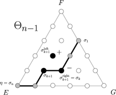
Figure 4. Three coplanar lines involved in the definition of a projective basis

As usual, put $\sigma_{k}=(\alpha_{k},\beta_{k},\gamma_{k})$. We begin by choosing a covector $u_{n}$ in the line $L_{\sigma_{n}}\subseteq V^{*}$, called a normalization. Having defined covectors $u_{n},u_{n-1},\dots,u_{k+1}$, we will define a covector

$$u_{k}\quad\in L_{\sigma_{k}}=\left(E^{(\alpha_{k})}\oplus F^{(\beta_{k})}\oplus G^{(\gamma_{k})}\right)^{\perp}\quad\subseteq V^{*}.$$

By the definition of snakes, we see that given $\sigma_{k+1}$ there are only two possibilities for $\sigma_{k}$, denoted either $\sigma_{k+1}^{\mathrm{left}}$ or $\sigma_{k+1}^{\mathrm{right}}$ depending on its coordinates:

$$\sigma_{k+1}^{\mathrm{left}} =(\alpha^{\mathrm{left}}_{k+1},\beta^{\mathrm{left}}_{k+1},\gamma^{\mathrm{left}}_{k+1}), \alpha^{\mathrm{left}}_{k+1} =k-1, \beta^{\mathrm{left}}_{k+1} =\beta_{k+1}+1, \gamma^{\mathrm{left}}_{k+1} =\gamma_{k+1};$$

$$\sigma_{k+1}^{\mathrm{right}} =(\alpha^{\mathrm{right}}_{k+1},\beta^{\mathrm{right}}_{k+1},\gamma^{\mathrm{right}}_{k+1}), \alpha^{\mathrm{right}}_{k+1} =k-1, \beta^{\mathrm{right}}_{k+1} =\beta_{k+1}, \gamma^{\mathrm{right}}_{k+1} =\gamma_{k+1}+1.$$

See Figure 4, where $\sigma_{k}=\sigma_{k+1}^{\mathrm{right}}$. Thus, the lines $L_{\sigma^{\mathrm{left}}_{k+1}}$ and $L_{\sigma^{\mathrm{right}}_{k+1}}$ can be written

$$\begin{split}L_{\sigma_{k+1}^{\mathrm{left}}}&=\left(E^{(k-1)}\oplus F^{(\beta_{k+1}+1)}\oplus G^{(\gamma_{k+1})}\right)^{\perp}\quad\subseteq V^{*};\\ L_{\sigma_{k+1}^{\mathrm{right}}}&=\left(E^{(k-1)}\oplus F^{(\beta_{k+1})}\oplus G^{(\gamma_{k+1}+1)}\right)^{\perp}\quad\subseteq V^{*}.\end{split}$$

It follows by the Maximum Span Property that the three lines $L_{\sigma_{k+1}}$, $L_{\sigma_{k+1}^{\mathrm{left}}}$, $L_{\sigma_{k+1}^{\mathrm{right}}}$ in $V^{*}$ are distinct and coplanar. Specifically, they lie in the plane

$$\left(E^{(k-1)}\oplus F^{(\beta_{k+1})}\oplus G^{(\gamma_{k+1})}\right)^{\perp}\quad\subseteq V^{*}$$

which is indeed 2-dimensional, since $(k+\beta_{k+1}+\gamma_{k+1})-1=(n-1)-1$. Thus, if $u_{k+1}$ is a nonzero covector in the line $L_{\sigma_{k+1}}$, then there exist unique nonzero covectors $u_{k+1}^{\mathrm{left}}$ and $u_{k+1}^{\mathrm{right}}$ in the lines $L_{\sigma_{k+1}^{\mathrm{left}}}$ and $L_{\sigma_{k+1}^{\mathrm{right}}}$, respectively, such that

$$u_{k+1}+u_{k+1}^{\mathrm{left}}+u_{k+1}^{\mathrm{right}}=0\quad\in V^{*}.$$

Definition 11.

Having chosen $u_{n}\in L_{\sigma_{n}}=L_{(n-1,0,0)}$ and having inductively defined $u_{k^{\prime}}\in L_{\sigma_{k^{\prime}}}$ for $k^{\prime}=n,n-1,\dots,k+1$, define $u_{k}\in L_{\sigma_{k}}$ by the formula

1. if $\sigma_{k}=\sigma_{k+1}^{\mathrm{left}}$, put $u_{k}=+u_{k+1}^{\mathrm{left}}\in L_{\sigma_{k+1}^{\mathrm{left}}}$;

2. if $\sigma_{k}=\sigma_{k+1}^{\mathrm{right}}$, put $u_{k}=-u_{k+1}^{\mathrm{right}}\in L_{\sigma_{k+1}^{\mathrm{right}}}$.

See Figure 4, which falls into the second case. Note if the initial choice of normalization $u_{n}$ is replaced by $\lambda u_{n}$ for some scalar $\lambda$, then $u_{k}$ is replaced by $\lambda u_{k}$ for all $1\leqslant k\leqslant n$. We gather this process produces a projective basis $[\mathscr{U}]=[\left\{u_{1},u_{2},\dots,u_{n}\right\}]$ of $V^{*}$, as desired.

1.4. Snake moves

1.4.1. Shearing (and U-turn) matrices

Let $\mathscr{A}$ be a commutative algebra, such as $\mathscr{A}=\mathbb{C}$. Let $X^{1/n},Z^{1/n}\in\mathscr{A}$, and put $X=(X^{1/n})^{n}$ and $Z=(Z^{1/n})^{n}$. Let $\mathrm{M}_{n}(\mathscr{A})$ (resp. $\mathrm{SL}_{n}(\mathscr{A})$) denote the usual ring of $n\times n$ matrices (resp. having determinant equal to 1) over $\mathscr{A}$ (see §2.1.2).

For $k=1,2,\dots,n-1$ define the $k$-th left-shearing matrix $\mathbf{S}^{\mathrm{left}}_{k}(X)\in\mathrm{SL}_{n}(\mathscr{A})$ by

$$\mathbf{S}^{\mathrm{left}}_{k}(X)=X^{-(k-1)/n}\left(\begin{smallmatrix}X&&&&&&&\\ &\ddots&&&&&&\\ &&X&&&&&\\ &&&1&1&&&\\ &&&&1&&&\\ &&&&&1&&\\ &&&&&&\ddots&\\ &&&&&&&1\end{smallmatrix}\right)\quad\in\mathrm{SL}_{n}(\mathscr{A})\quad\quad\left(X\text{ appears }k-1\text{ times}\right),$$

and define the $k$-th right-shearing matrix $\mathbf{S}^{\mathrm{right}}_{k}(X)\in\mathrm{SL}_{n}(\mathscr{A})$ by

$$\mathbf{S}^{\mathrm{right}}_{k}(X)=X^{+(k-1)/n}\left(\begin{smallmatrix}1&&&&&&&\\ &\ddots&&&&&&\\ &&1&&&&&\\ &&&1&&&\\ &&&1&1&&&\\ &&&&&X^{-1}&&\\ &&&&&&\ddots&\\ &&&&&&&X^{-1}\end{smallmatrix}\right)\quad\in\mathrm{SL}_{n}(\mathscr{A})\quad\quad\left(X\text{ appears }k-1\text{ times}\right).$$

Note that $\mathbf{S}^{\mathrm{left}}_{1}(X)$ and $\mathbf{S}^{\mathrm{right}}_{1}(X)$ do not, in fact, involve the variable $X$, and so we will denote these matrices simply by $\mathbf{S}^{\mathrm{left}}_{1}$ and $\mathbf{S}^{\mathrm{right}}_{1}$, respectively.

For $j=1,2,\dots,n-1$ define the $j$-th edge-shearing matrix $\mathbf{S}^{\mathrm{edge}}_{j}(Z)\in\mathrm{SL}_{n}(\mathscr{A})$ by

$$\mathbf{S}^{\mathrm{edge}}_{j}(Z)=Z^{-j/n}\left(\begin{smallmatrix}Z&&&&&&&\\ &Z&&&&&&\\ &&\ddots&&&&&\\ &&&Z&&&&\\ &&&&1&&&\\ &&&&&1&&\\ &&&&&&\ddots&\\ &&&&&&&1\end{smallmatrix}\right)\quad\in\mathrm{SL}_{n}(\mathscr{A})\quad\quad\left(Z\text{ appears }j\text{ times}\right).$$

Lastly, define the clockwise U-turn matrix $\mathbf{U}$ in $\mathrm{SL}_{n}(\mathbb{C})$ by

$$\mathbf{U}=\left(\begin{smallmatrix}&&&&\\ &&&&(-1)^{n-1}\\ &&&\reflectbox{$\ddots$}&\\ &&+1&&\\ &-1&&&\\ +1&&&&\end{smallmatrix}\right)\quad\in\mathrm{SL}_{n}(\mathbb{C}).$$

1.4.2. Adjacent snake pairs

Definition 12.

We say that an ordered pair $(\sigma,\sigma^{\prime})$ of snakes $\sigma$ and $\sigma^{\prime}$ forms an adjacent pair of snakes if the pair $(\sigma,\sigma^{\prime})$ satisfies either of the following conditions:

1. for some $2\leqslant k\leqslant n-1$,

   1. $\sigma_{j}=\sigma^{\prime}_{j}$             $(1\leqslant j\leqslant k-1$,  $k+1\leqslant j\leqslant n)$,

   2. $\sigma_{k}=\sigma_{k+1}^{\mathrm{right}}\,\,(=\sigma_{k+1}^{\prime\mathrm{right}}),$  and  $\sigma^{\prime}_{k}=\sigma_{k+1}^{\mathrm{left}}\,\,(=\sigma_{k+1}^{\prime\mathrm{left}})$,

   in which case $(\sigma,\sigma^{\prime})$ is called an adjacent pair of diamond-type, see Figure 5;

2. 1. $\sigma_{j}=\sigma^{\prime}_{j}$             $(2\leqslant j\leqslant n)$,

   2. $\sigma_{1}=\sigma_{2}^{\mathrm{right}}\,\,(=\sigma_{2}^{\prime\mathrm{right}})$,  and  $\sigma^{\prime}_{1}=\sigma_{2}^{\mathrm{left}}\,\,(=\sigma_{2}^{\prime\mathrm{left}})$,

   in which case $(\sigma,\sigma^{\prime})$ is called an adjacent pair of tail-type, see Figure 6.

1.4.3. Diamond and tail moves

Until we arrive at the next proposition, let $(\sigma,\sigma^{\prime})$ be an adjacent pair of snakes of diamond-type, as shown in Figure 5.

Consider the snake-vertices $\sigma_{k+1}$ $(=\sigma^{\prime}_{k+1})$, $\sigma_{k}$, $\sigma^{\prime}_{k}$, and $\sigma_{k-1}$ $(=\sigma^{\prime}_{k-1})$. One checks that

$$\alpha_{k}=\alpha^{\prime}_{k}\quad=k-1,\quad\quad\beta_{k}^{\prime}=\beta_{k-1}\quad=\beta_{k+1}+1,\quad\quad\gamma_{k}=\gamma_{k-1}\quad=\gamma_{k+1}+1.$$

Taken together, these three coordinates form a vertex

$$(a,b,c)\quad=(k-1,\beta_{k+1}+1,\gamma_{k+1}+1)\quad\in\mathrm{int}(\Theta_{n})$$

in the interior of the $n$-discrete triangle $\Theta_{n}$ (not $\Theta_{n-1}$). The coordinates of this internal vertex $(a,b,c)$ can also be thought of as delineating the boundary of a small downward-facing triangle $\nabla$ in the discrete triangle $\Theta_{n-1}$, whose three vertices are $\sigma_{k},\sigma^{\prime}_{k}$, $\sigma_{k-1}$ (Figure 5). Put $X_{abc}=\tau_{abc}(E,F,G)\in\mathbb{C}-\left\{0\right\}$, namely $X_{abc}$ is the Fock-Goncharov triangle invariant (§1.2.4) associated to the generic flag triple $(E,F,G)$ and the internal vertex $(a,b,c)\in\mathrm{int}(\Theta_{n})$.

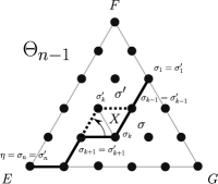
Figure 5. Diamond move

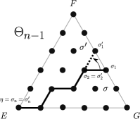
Figure 6. Tail move

The following result is the main ingredient going into the proof of Theorem 7.

Proposition 13.

Let $(E,F,G)$ be a maximum span flag triple, $(\sigma,\sigma^{\prime})$ an adjacent pair of snakes, and $\mathscr{U}$, $\mathscr{U}^{\prime}$ the corresponding normalized projective bases of $V^{*}$ so that $u_{n}=u^{\prime}_{n}\in L_{\sigma_{n}}$.

If $(\sigma,\sigma^{\prime})$ is of diamond-type, then the change of basis matrix $\mathbf{B}_{\mathscr{U}\to\mathscr{U}^{\prime}}\in\mathrm{GL}_{n}(\mathbb{C})$ (§1.1.2) is

$$\mathbf{B}_{\mathscr{U}\to\mathscr{U}^{\prime}}=X_{abc}^{+(k-1)/n}\,\mathbf{S}_{k}^{\mathrm{left}}(X_{abc})\quad\in\mathrm{GL}_{n}(\mathbb{C})\quad\quad(\text{see }\S\ref{sec:theorem-3}).$$

We say this case expresses a diamond move from the snake $\sigma$ to the adjacent snake $\sigma^{\prime}$.

If $(\sigma,\sigma^{\prime})$ is of tail-type, then the change of basis matrix $\mathbf{B}_{\mathscr{U}\to\mathscr{U}^{\prime}}$ equals

$$\mathbf{B}_{\mathscr{U}\to\mathscr{U}^{\prime}}=\mathbf{S}_{1}^{\mathrm{left}}\quad\in\mathrm{SL}_{n}(\mathbb{C}).$$

We say this case expresses a tail move from the snake $\sigma$ to the adjacent snake $\sigma^{\prime}$.

Proof.

See [FG06b, §9]. We also provide a proof in [Dou20, §2.18]. ∎

1.4.4. Right snakes and right snake moves

Our definition of a (left) snake in §1.3.1 took the snake-head $\eta=\sigma_{n}$ to be the $n$-th snake-vertex. There is another possibility, where $\eta=\sigma_{1}$:

Definition 14.

A right $n$-snake $\sigma$ (for the snake-head $\eta=(n-1,0,0)\in\Gamma(\Theta_{n-1})$) is a sequence $\sigma=(\sigma_{1},\sigma_{2},\dots,\sigma_{n})\in(\Theta_{n-1})^{n}$ of $n$-many vertices $\sigma_{k}=(\alpha_{k},\beta_{k},\gamma_{k})$, satisfying

$$\alpha_{k}=n-k,\quad\quad\beta_{k}\geqslant\beta_{k-1},\quad\quad\gamma_{k}\geqslant\gamma_{k-1}\quad\quad\left(k=1,2,\dots,n\right).$$

Right snakes for other snake-heads $\eta\in\Gamma(\Theta_{n-1})$ are similarly defined by triangular symmetry.

To adjust for using right snakes, the definitions of §1.3.3, 1.4.2, 1.4.3 need to be modified.

Given $\sigma_{k-1}$, there are two possibilities for $\sigma_{k}$:

$$\sigma_{k-1}^{\mathrm{left}} =(\alpha^{\mathrm{left}}_{k-1},\beta^{\mathrm{left}}_{k-1},\gamma^{\mathrm{left}}_{k-1}), \alpha^{\mathrm{left}}_{k-1} =n-k, \beta^{\mathrm{left}}_{k-1} =\beta_{k-1}+1, \gamma^{\mathrm{left}}_{k-1} =\gamma_{k-1};$$

$$\sigma_{k-1}^{\mathrm{right}} =(\alpha^{\mathrm{right}}_{k-1},\beta^{\mathrm{right}}_{k-1},\gamma^{\mathrm{right}}_{k-1}), \alpha^{\mathrm{right}}_{k-1} =n-k, \beta^{\mathrm{right}}_{k-1} =\beta_{k-1}, \gamma^{\mathrm{right}}_{k-1} =\gamma_{k-1}+1.$$

The algorithm defining the (ordered) projective basis $[\mathscr{U}]=[\left\{u_{1},u_{2},\dots,u_{n}\right\}]$ becomes:

1. if $\sigma_{k}=\sigma_{k-1}^{\mathrm{left}}$, put $u_{k}=-u_{k-1}^{\mathrm{left}}\in L_{\sigma_{k-1}^{\mathrm{left}}}$;

2. if $\sigma_{k}=\sigma_{k-1}^{\mathrm{right}}$, put $u_{k}=+u_{k-1}^{\mathrm{right}}\in L_{\sigma_{k-1}^{\mathrm{right}}}$.

In particular, the algorithm starts by making a choice of covector $u_{1}\in L_{\sigma_{1}}=L_{(n-1,0,0)}$. Notice that, compared to the setting of left snakes (Definition 11 and Figure 4), the signs defining the projective basis have been swapped.

An ordered pair $(\sigma,\sigma^{\prime})$ of right snakes forms an adjacent pair if either:

1. for some $2\leqslant k\leqslant n-1$,

   1. $\sigma_{j}=\sigma^{\prime}_{j}$             $(1\leqslant j\leqslant k-1$,  $k+1\leqslant j\leqslant n)$,

   2. $\sigma_{k}=\sigma_{k-1}^{\mathrm{left}}\,\,(=\sigma_{k-1}^{\prime\mathrm{left}}),$  and  $\sigma^{\prime}_{k}=\sigma_{k-1}^{\mathrm{right}}\,\,(=\sigma_{k-1}^{\prime\mathrm{right}})$,

   in which case $(\sigma,\sigma^{\prime})$ is called an adjacent pair of diamond-type;

2. 1. $\sigma_{j}=\sigma^{\prime}_{j}$             $(1\leqslant j\leqslant n-1)$,

   2. $\sigma_{n}=\sigma_{n-1}^{\mathrm{left}}\,\,(=\sigma_{n-1}^{\prime\mathrm{left}})$,  and  $\sigma^{\prime}_{n}=\sigma_{n-1}^{\mathrm{right}}\,\,(=\sigma_{n-1}^{\prime\mathrm{right}})$,

   in which case $(\sigma,\sigma^{\prime})$ is called an adjacent pair of tail-type.

Given an adjacent pair $(\sigma,\sigma^{\prime})$ of right snakes of diamond-type, there is naturally associated a vertex $(a,b,c)\in\Theta_{n}$ to which is assigned a Fock-Goncharov triangle invariant $X_{abc}$.

Proposition 15.

Let $(E,F,G)$ be a maximum span triple, $(\sigma,\sigma^{\prime})$ an adjacent pair of right snakes, and $\mathscr{U}$, $\mathscr{U}^{\prime}$ the corresponding normalized projective bases of $V^{*}$ so that $u_{1}=u^{\prime}_{1}\in L_{\sigma_{1}}$.

If $(\sigma,\sigma^{\prime})$ is of diamond-type, then the change of basis matrix $\mathbf{B}_{\mathscr{U}\to\mathscr{U}^{\prime}}\in\mathrm{GL}_{n}(\mathbb{C})$ equals

$$\mathbf{B}_{\mathscr{U}\to\mathscr{U}^{\prime}}=X_{abc}^{-(k-1)/n}\,\mathbf{S}_{k}^{\mathrm{right}}(X_{abc})\quad\in\mathrm{GL}_{n}(\mathbb{C})\quad\quad(\text{see }\S\ref{sec:theorem-3}).$$

If $(\sigma,\sigma^{\prime})$ is of tail-type, then the change of basis matrix $\mathbf{B}_{\mathscr{U}\to\mathscr{U}^{\prime}}$ equals

$$\mathbf{B}_{\mathscr{U}\to\mathscr{U}^{\prime}}=\mathbf{S}_{1}^{\mathrm{right}}\quad\in\mathrm{SL}_{n}(\mathbb{C}).$$

Proof.

See [FG06b, §9]. Similar to the proof of Proposition 13. ∎

Remark 16.

From now on, “snake” means “left snake”, as in Definition 10, and we will say explicitly if we are using “right snakes”.

1.4.5. Snake moves for edges

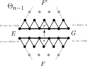
Figure 7. Edge move

Let $(E,G,F,F^{\prime})$ be a maximum span flag quadruple; see §1.2.2. By §1.2.4, for each $j=1,\dots,n-1$ we may consider the Fock-Goncharov edge invariant $Z_{j}=\epsilon_{j}(E,G,F,F^{\prime})\in\mathbb{C}-\left\{0\right\}$ associated to the quadruple $(E,G,F,F^{\prime})$.

Warning: In this subsubsection, we will consider snake-heads $\eta$ in the set of corner vertices $\left\{(n-1,0,0),(0,n-1,0),(0,0,n-1)\right\}$ other than $\eta=(n-1,0,0)$; see Remark 9.

Consider two copies of the discrete triangle; Figure 7. The bottom triangle $\Theta_{n-1}(G,F,E)$ has a maximum span flag triple $(G,F,E)$ assigned to the corner vertices $\Gamma(\Theta_{n-1})$, and the top triangle $\Theta_{n-1}(E,F^{\prime},G)$ has assigned to $\Gamma(\Theta_{n-1})$ a maximum span flag triple $(E,F^{\prime},G)$.

Define two snakes $\sigma$ and $\sigma^{\prime}$ in $\Theta_{n-1}(G,F,E)$ and $\Theta_{n-1}(E,F^{\prime},G)$, respectively, as follows:

$$\sigma_{k} =(n-k,0,k-1) \in\Theta_{n-1}(G,F,E) \left(k=1,\dots,n\right);$$

$$\sigma^{\prime}_{k} =(k-1,0,n-k) \in\Theta_{n-1}(E,F^{\prime},G) \left(k=1,\dots,n\right).$$

Notice that the line decompositions associated to the snakes $\sigma$ and $\sigma^{\prime}$ are the same:

$$L_{\sigma_{k}}=L_{\sigma^{\prime}_{k}}=\left(E^{(k-1)}\oplus G^{(n-k)}\right)^{\perp}\quad\subseteq V^{*}\quad\quad\left(k=1,\dots,n\right).$$

Normalize the two associated projective bases $[\mathscr{U}]$ and $[\mathscr{U}^{\prime}]$ by choosing $u_{n}=u^{\prime}_{n}$ in $L_{\sigma_{n}}=L_{\sigma^{\prime}_{n}}$.

Proposition 17.

The change of basis matrix expressing the snake move $\sigma\to\sigma^{\prime}$ is

$$\mathbf{B}_{\mathscr{U}\to\mathscr{U}^{\prime}}=\prod_{j=1}^{n-1}Z_{j}^{+j/n}\,\mathbf{S}_{j}^{\mathrm{edge}}(Z_{j})\quad\in\mathrm{GL}_{n}(\mathbb{C})\quad\quad(\text{see }\S\ref{sec:theorem-3}).$$

Proof.

See [FG06b, §9]. Similar to the proof of Proposition 13; see also [Dou20, §2.22]. ∎

Next, define snakes $\sigma$ and $\sigma^{\prime}$ in a single discrete triangle $\Theta_{n-1}(E,F,G)$ by (see Figure 8)

$$\sigma_{k} =(n-k,0,k-1) \in\Theta_{n-1} \left(k=1,\dots,n\right);$$

$$\sigma^{\prime}_{k} =(k-1,0,n-k) \in\Theta_{n-1} \left(k=1,\dots,n\right).$$

Notice that the lines $L_{\sigma_{k}}\neq L_{\sigma^{\prime}_{k}}$ in $V^{*}$ are not equal. In fact, $L_{\sigma_{k}}=L_{\sigma^{\prime}_{n-k+1}}$. Normalize the two associated projective bases $[\mathscr{U}]$ and $[\mathscr{U}^{\prime}]$ by choosing $u_{n}=u^{\prime}_{1}$ in $L_{\eta}=L_{\sigma_{n}}=(G^{(n-1)})^{\perp}$.

Proposition 18.

The change of basis matrix expressing the snake move $\sigma\to\sigma^{\prime}$ is

$$\mathbf{B}_{\mathscr{U}\to\mathscr{U}^{\prime}}=\mathbf{U}\quad\in\mathrm{SL}_{n}(\mathbb{C})\quad\quad(\text{see }\S\ref{sec:theorem-3}).$$

Proof.

See [FG06b, §9]. Similar to the proof of Proposition 13; see also [Dou20, §2.22]. ∎

Remark 19.

This last U-turn move will not be needed in this paper, but appears in [Dou21].

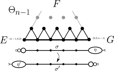
Figure 8. Clockwise U-turn Move

1.5. Triangle and edge invariants as shears

This subsection does not involves snakes. A line $L$ (resp. plane $P$) in $V^{*}$ is a 1-dimensional (resp. 2-dimensional) subspace of $V^{*}$.

Definition 20.

A shear $S$ from a line $L_{1}$ in $V^{*}$ to another line $L_{2}$ in $V^{*}$ is simply a linear isomorphism $S:L_{1}\to L_{2}$.

1.5.1. Triangle invariants as shears

Let $(E,F,G)$ be a maximum span flag triple, and consider an internal vertex $(a,b,c)\in\mathrm{int}(\Theta_{n})$ in the $n$-discrete triangle. As in §1.4.3, the level sets in $\Theta_{n-1}$ defined by the equations $\alpha=a$, $\beta=b$, $\gamma=c$ delineate the boundary of a downward-facing triangle $\nabla$ with vertices $\nu_{1}^{\prime},\nu_{2}^{\prime},\nu_{3}^{\prime}$, which is centered in a larger upward-facing triangle $\Delta$ with vertices $\nu_{1}$, $\nu_{2}$, $\nu_{3}$; see Figure 9. There are also three smaller upward-facing triangles $\Delta_{1}$, $\Delta_{2}$, $\Delta_{3}$ defined by their vertices:

$$\Delta_{1}=\left\{\nu_{1},\nu^{\prime}_{3},\nu^{\prime}_{2}\right\},\quad\quad\Delta_{2}=\left\{\nu_{2},\nu^{\prime}_{1},\nu^{\prime}_{3}\right\},\quad\quad\Delta_{3}=\left\{\nu_{3},\nu^{\prime}_{2},\nu^{\prime}_{1}\right\}.$$

Given one of these small upward-facing triangles, say $\Delta_{1}$, the crucial property we used to define projective bases in §1.3.3 is that the three lines $L_{\nu_{1}}$, $L_{\nu^{\prime}_{3}}$, $L_{\nu^{\prime}_{2}}$ in $V^{*}$ attached to the vertices of $\Delta_{1}$ are coplanar. Consequently, to the triangle $\Delta_{1}$ there are associated six shears: $S^{\Delta_{1}}_{\nu_{1}\nu^{\prime}_{3}}:L_{\nu_{1}}\to L_{\nu^{\prime}_{3}}$ and $S^{\Delta_{1}}_{\nu^{\prime}_{3}\nu^{\prime}_{2}}:L_{\nu^{\prime}_{3}}\to L_{\nu^{\prime}_{2}}$ and $S^{\Delta_{1}}_{\nu^{\prime}_{2}\nu_{1}}:L_{\nu^{\prime}_{2}}\to L_{\nu_{1}}$ and their inverses. For instance, the shear $S^{\Delta_{1}}_{\nu_{1}\nu^{\prime}_{3}}$ sends a point $p$ in $L_{\nu_{1}}$ to the unique point $p^{\prime}$ in $L_{\nu^{\prime}_{3}}$ such that

$$p+p^{\prime}+p^{\prime\prime}=0\quad\in V^{*}$$

for some (unique) point $p^{\prime\prime}\in L_{\nu^{\prime}_{2}}$. And $S^{\Delta_{1}}_{\nu_{1}\nu^{\prime}_{2}}(p)=p^{\prime\prime}$. Similarly for the other triangles $\Delta_{2},\Delta_{3}$.

Let $X_{abc}=\tau_{abc}(E,F,G)$ be the triangle invariant associated to the vertex $(a,b,c)$.

Proposition 21.

Fix a point $p_{0}$ in the line $L_{\nu^{\prime}_{1}}$. Let $p_{1}$ be the point in the line $L_{\nu^{\prime}_{3}}$ resulting from the shear $S^{\Delta_{2}}_{\nu^{\prime}_{1}\nu^{\prime}_{3}}$ associated to the triangle $\Delta_{2}$ applied to the point $p_{0}$, let $p_{2}$ be the point in the line $L_{\nu^{\prime}_{2}}$ resulting from the shear $S^{\Delta_{1}}_{\nu^{\prime}_{3}\nu^{\prime}_{2}}$ associated to the triangle $\Delta_{1}$ applied to the point $p_{1}$, and let $p_{3}$ be the point in the line $L_{\nu^{\prime}_{1}}$ resulting from the shear $S^{\Delta_{3}}_{\nu^{\prime}_{2}\nu^{\prime}_{1}}$ associated to the triangle $\Delta_{3}$ applied to the point $p_{2}$. It follows that

$$p_{3}=+X_{abc}\,p_{0}.$$

This was the case going counterclockwise around the $(a,b,c)$-downward-facing triangle $\nabla$; see Figure 9. If instead one goes clockwise around $\nabla$, then the total shearing is $+X_{abc}^{-1}$.

Proof.

See [FG06b, GMN14]. Similar to that of Proposition 13; see also [Dou20, §2.21]. ∎

1.5.2. Edge invariants as shears

Similarly, consider two discrete triangles $\Theta_{n-1}(E,F^{\prime},G)$ and $\Theta_{n-1}(G,F,E)$ as in the first half of §1.4.5, the edge invariant $Z_{j}=\epsilon_{j}(E,G,F,F^{\prime})$ for $j=1,\dots,n-1$, and two small upward-facing (relatively speaking) triangles $\Delta^{\prime}$ and $\nabla$ in $\Theta_{n-1}(E,F^{\prime},G)$ and $\Theta_{n-1}(G,F,E)$, respectively, as shown in Figure 10.

Proposition 22.

Fix a point $p_{0}$ in the line $L_{\nu^{\prime}_{0}}(E,F^{\prime},G)$. Let $p_{1}$ be the point in the line $L_{\nu_{1}^{\prime}}(E,F^{\prime},G)=L_{\nu_{1}}(G,F,E)$ resulting from the shear $S^{\Delta^{\prime}}_{\nu_{0}^{\prime}\nu^{\prime}_{1}}$ associated to the triangle $\Delta^{\prime}$ applied to the point $p_{0}$, and let $p_{2}$ be the point in the line $L_{\nu_{0}}(G,F,E)=L_{\nu^{\prime}_{0}}(E,F^{\prime},G)$ resulting from the shear $S^{\nabla}_{\nu_{1}\nu_{0}}$ associated to the triangle $\nabla$ applied to the point $p_{1}$. Then

$$p_{2}=-Z_{j}\,p_{0}.$$

This was the case going counterclockwise around the $j$-th diamond; see Figure 10. If instead one goes clockwise around the diamond, then the total shearing is $-Z_{j}^{-1}$.

Proof.

See [FG06b, GMN14]. Similar to that of Proposition 13; see also [Dou20, §2.23]. ∎

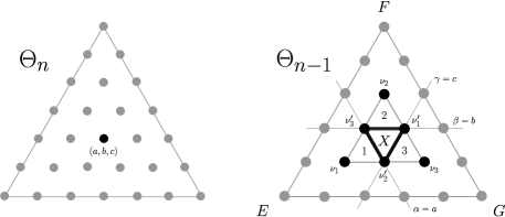
Figure 9. Triangle invariants as shears

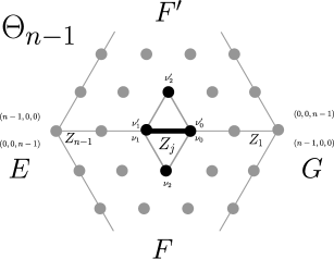
Figure 10. Edge invariants as shears

1.6. Classical left, right, and edge matrices

We begin the process of algebraizing the geometry discussed throughout §1.

Warning: In this subsection, we will consider snake-heads $\eta$ in the set of corner vertices $\left\{(n-1,0,0),(0,n-1,0),(0,0,n-1)\right\}$ other than $\eta=(n-1,0,0)$; see Remark 9. We will also consider both (left) snakes and right snakes; see Remark 16.

1.6.1. Snake sequences

For the left setting: define a snake-head $\eta\in\Gamma(\Theta_{n-1})$ and two (left) snakes $\sigma^{\mathrm{bot}}$, $\sigma^{\mathrm{top}}$, called the bottom and top snakes, respectively, by

$$\eta=(n-1,0,0),\quad\sigma^{\mathrm{bot}}_{k}=(k-1,0,n-k),\quad\sigma^{\mathrm{top}}_{k}=(k-1,n-k,0)\quad\left(k=1,\dots,n\right).$$

See Figure 11. Similarly, for the right setting: define $\eta$ and right snakes $\sigma^{\mathrm{bot}}$, $\sigma^{\mathrm{top}}$ by

$$\eta=(0,0,n-1),\quad\sigma^{\mathrm{bot}}_{k}=(k-1,0,n-k),\quad\sigma^{\mathrm{top}}_{k}=(0,k-1,n-k)\quad\left(k=1,\dots,n\right).$$

In either left or right setting, consider a sequence $\sigma^{\mathrm{bot}}=\sigma^{1},\sigma^{2},\cdots,\sigma^{N-1},\sigma^{N}=\sigma^{\mathrm{top}}$ of snakes having the same snake-head $\eta$ as do $\sigma^{\mathrm{bot}}$ and $\sigma^{\mathrm{top}}$, such that $(\sigma^{\ell},\sigma^{\ell+1})$ is an adjacent pair; see Figure 11. Note that this sequence of snakes is not in general unique. For the $N$-many projective bases $[\mathscr{U}^{\ell}]=[\left\{u^{\ell}_{1},u^{\ell}_{2},\dots,u^{\ell}_{n}\right\}]$ associated to the snakes $\sigma^{\ell}$, choose a common normalization $u_{n}^{\ell}=u_{n}\in L_{\eta}$ (resp. $u_{1}^{\ell}=u_{1}\in L_{\eta}$) when working in the left (resp. right) setting. Then, the change of basis matrix $\mathbf{B}_{\mathscr{U}^{\mathrm{bot}}\to\mathscr{U}^{\mathrm{top}}}$ can be decomposed as (see §1.1.2)

($$\ast \mathbf{B}_{\mathscr{U}^{\mathrm{bot}}\to\mathscr{U}^{\mathrm{top}}}=\mathbf{B}_{\mathscr{U}^{1}\to\mathscr{U}^{2}}\mathbf{B}_{\mathscr{U}^{2}\to\mathscr{U}^{3}}\cdots\mathbf{B}_{\mathscr{U}^{N-1}\to\mathscr{U}^{N}}\quad\in\mathrm{GL}_{n}(\mathbb{C}).$$)

Here, the matrices $\mathbf{B}_{\mathscr{U}^{\ell}\to\mathscr{U}^{\ell+1}}$ are computed in Proposition 13 (resp. Proposition 15) in the left (resp. right) setting, and in particular are completely determined by the triangle invariants $X_{abc}\in\mathbb{C}-\left\{0\right\}$ associated to the internal vertices $(a,b,c)\in\mathrm{int}(\Theta_{n})$ of the $n$-discrete triangle.

Of course, the matrix $\mathbf{B}_{\mathscr{U}^{\mathrm{bot}}\to\mathscr{U}^{\mathrm{top}}}$ is by definition independent of the choice of snake sequence $(\sigma^{\ell})_{\ell}$. For concreteness, we will make a preferred choice of such sequence, depending on whether we are in the left or right setting; these two choices are illustrated in Figure 11.

(a) Left snake sequence (preferred choice)

(b) Right snake sequence (preferred choice)

Figure 11. Classical snake sweep ($n=5$)

1.6.2. Algebraization

Let $\mathscr{A}$ be a commutative algebra (§1.4.1). For $i=1,2,\dots,(n-1)(n-2)/2$, let $X_{i}^{1/n}\in\mathscr{A}$ and put $X_{i}=(X_{i}^{1/n})^{n}$. For $j=1,2,\dots,n-1$, let $Z_{j}^{1/n}\in\mathscr{A}$ and put $Z_{j}=(Z_{j}^{1/n})^{n}$. Note that $(n-1)(n-2)/2$ is the number of triangle invariants $X_{i}=\tau_{abc}(E,F,G)$, and $n-1$ is the number of edge invariants $Z_{j}=\epsilon_{j}(E,G,F,F^{\prime})$ on a single edge.

As a notational convention, given a family $\mathbf{M}_{\ell}\in\mathrm{M}_{n}(\mathscr{A})$ of $n\times n$ matrices, put

$$\begin{split}\prod_{\ell=m}^{p}\mathbf{M}_{\ell}&=\mathbf{M}_{m}\mathbf{M}_{m+1}\cdots\mathbf{M}_{p},\quad\quad\prod_{\ell=p+1}^{m}\mathbf{M}_{\ell}=1\quad\quad\left(m\leqslant p\right),\\ \coprod_{\ell=p}^{m}\mathbf{M}_{\ell}&=\mathbf{M}_{p}\mathbf{M}_{p-1}\cdots\mathbf{M}_{m},\quad\quad\coprod_{\ell=m-1}^{p}\mathbf{M}_{\ell}=1\quad\quad\left(m\leqslant p\right).\end{split}$$

Definition 23.

The left matrix $\mathbf{M}^{\mathrm{left}}(X_{i}\text{'s})$ in $\mathrm{SL}_{n}(\mathscr{A})$ is defined by

$$\mathbf{M}^{\mathrm{left}}(X_{i}\text{'s})=\coprod_{k=n-1}^{1}\left(\mathbf{S}^{\mathrm{left}}_{1}\prod_{\ell=2}^{k}\mathbf{S}^{\mathrm{left}}_{\ell}\left(X_{(\ell-1)(n-k)(k-\ell+1)}\right)\right)\quad\in\mathrm{SL}_{n}(\mathscr{A})$$

where the matrix $\mathbf{S}_{\ell}^{\mathrm{left}}(X_{abc})$ is the $\ell$-th left-shearing matrix; see §1.4.1.

Similarly, the right matrix $\mathbf{M}^{\mathrm{right}}(X_{i}\text{'s})$ in $\mathrm{SL}_{n}(\mathscr{A})$ is defined by

$$\mathbf{M}^{\mathrm{right}}(X_{i}\text{'s})=\coprod_{k=n-1}^{1}\left(\mathbf{S}^{\mathrm{right}}_{1}\prod_{\ell=2}^{k}\mathbf{S}^{\mathrm{right}}_{\ell}\left(X_{(k-\ell+1)(n-k)(\ell-1)}\right)\right)\quad\in\mathrm{SL}_{n}(\mathscr{A})$$

where the matrix $\mathbf{S}_{\ell}^{\mathrm{right}}(X_{abc})$ is the $\ell$-th right-shearing matrix; see §1.4.1.

Lastly, the edge matrix $\mathbf{M}^{\mathrm{edge}}(Z_{j}\text{'s})$ in $\mathrm{SL}_{n}(\mathscr{A})$ is defined by

$$\mathbf{M}^{\mathrm{edge}}(Z_{j}\text{'s})=\prod_{\ell=1}^{n-1}\mathbf{S}^{\mathrm{edge}}_{\ell}(Z_{\ell})\quad\in\mathrm{SL}_{n}(\mathscr{A})$$

where the matrix $\mathbf{S}_{\ell}^{\mathrm{edge}}(Z_{\ell})$ is the $\ell$-th edge-shearing matrix; see §1.4.1. See Figure 12.

Remark 24.

In the case where $\mathscr{A}=\mathbb{C}$ and the $X_{i}=\tau_{abc}(E,F,G)$ and $Z_{j}=\epsilon_{j}(E,G,F,F^{\prime})$ in $\mathbb{C}-\left\{0\right\}$ are the triangle and edge invariants (as in §1.4.3, 1.4.4, 1.4.5): then, the left and right matrices $\mathbf{M}^{\mathrm{left}}(X_{i}\text{'s})$ and $\mathbf{M}^{\mathrm{right}}(X_{i}\text{'s})$ recover the change of basis matrix $\mathbf{B}_{\mathscr{U}^{\mathrm{bot}}\to\mathscr{U}^{\mathrm{top}}}/\mathrm{Det}^{1/n}$ of Eq. ($\ast$ ‣ 1.6.1) in the left and right setting, respectively, normalized to have determinant 1, and decomposed in terms of our preferred snake sequence (Figure 11); and, the edge matrix $\mathbf{M}^{\mathrm{edge}}(Z_{j}\text{'s})$ is the normalization $\mathbf{B}_{\mathscr{U}\to\mathscr{U}^{\prime}}/\mathrm{Det}^{1/n}$ of the change of basis matrix from Proposition 17. Crucially, these normalizations require choosing $n$-roots of the invariants $X_{i}$ and $Z_{j}$.

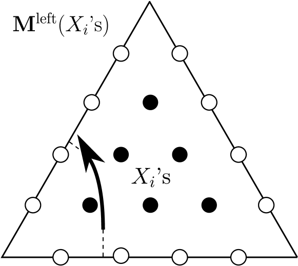
(a) Left matrix

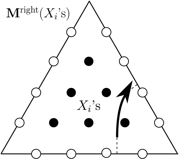
(b) Right matrix

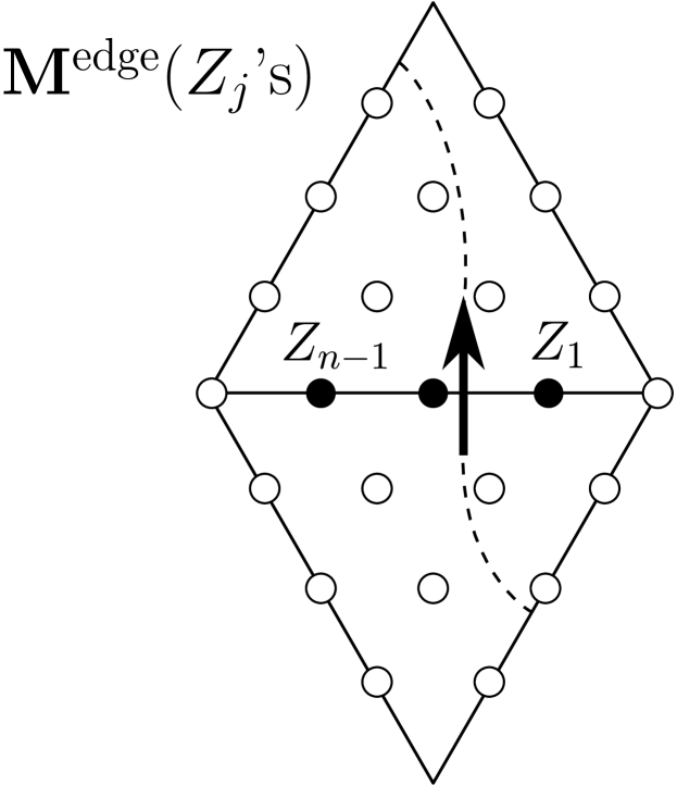
(c) Edge matrix

Figure 12. Classical matrices (viewed from the $\Theta_{n}$-perspective)

2. Quantum matrices

Although we will not use explicitly the geometric results of the previous section, those results motivate the algebraic objects that are the main focus of the present work.

Throughout, let $q\in\mathbb{C}-\left\{0\right\}$ and $\omega=q^{1/n^{2}}$ be a $n^{2}$-root of $q$. Technically, also choose $\omega^{1/2}$.

2.1. Quantum tori, matrix algebras, and the Weyl quantum ordering

2.1.1. Quantum tori

Let $\mathbf{P}$ (for “Poisson”) be an integer $N^{\prime}\times N^{\prime}$ anti-symmetric matrix.

Definition 25.

The quantum torus (with $n$-roots) $\mathscr{T}^{\omega}(\mathbf{P})$ associated to $\mathbf{P}$ is the quotient of the free algebra $\mathbb{C}\{X_{1}^{1/n},X_{1}^{-1/n},\dots,X_{N^{\prime}}^{1/n},X_{N^{\prime}}^{-1/n}\}$ in the indeterminates $X_{i}^{\pm 1/n}$ by the two-sided ideal generated by the relations

$$X_{i}^{m_{i}/n}X_{j}^{m_{j}/n}=\omega^{\mathbf{P}_{ij}m_{i}m_{j}}X_{j}^{m_{j}/n}X_{i}^{m_{i}/n}\quad\quad(m_{i},m_{j}\in\mathbb{Z}),$$

$$X_{i}^{m/n}X_{i}^{-{m/n}}=X_{i}^{-{m/n}}X_{i}^{m/n}=1\quad\quad(m\in\mathbb{Z}).$$

Put $X_{i}^{\pm 1}=(X_{i}^{\pm 1/n})^{n}$. We refer to the $X_{i}^{\pm 1/n}$ as generators, and the $X_{i}$ as quantum coordinates, or just coordinates. Define the subset of fractions

$$\mathbb{Z}/n=\left\{{m/n};\quad m\in\mathbb{Z}\right\}\quad\subseteq\mathbb{Q}.$$

Written in terms of the coordinates $X_{i}$ and the fractions $r\in\mathbb{Z}/n$, the relations above become

$$X_{i}^{r_{i}}X_{j}^{r_{j}}=q^{\mathbf{P}_{ij}r_{i}r_{j}}X_{j}^{r_{j}}X_{i}^{r_{i}}\quad\quad(r_{i},r_{j}\in\mathbb{Z}/n),$$

$$X_{i}^{r}X_{i}^{-r}=X_{i}^{-r}X_{i}^{r}=1\quad\quad(r\in\mathbb{Z}/n).$$

2.1.2. Matrix algebras

Definition 26.

Let $\mathscr{T}$ be a, possibly non-commutative, complex algebra, and let $n^{\prime}$ be a positive integer. The matrix algebra with coefficients in $\mathscr{T}$, denoted $\mathrm{M}_{n^{\prime}}(\mathscr{T})$, is the complex vector space of $n^{\prime}\times n^{\prime}$ matrices, equipped with the usual “left-to-right” multiplicative structure. Namely, the product $\mathbf{M}\mathbf{N}$ of two matrices $\mathbf{M}$ and $\mathbf{N}$ is defined entry-wise by

$$(\mathbf{M}\mathbf{N})_{ij}=\sum_{k=1}^{n^{\prime}}\mathbf{M}_{ik}\mathbf{N}_{kj}\quad\in\mathscr{T}\quad\quad\left(1\leqslant i,j\leqslant n^{\prime}\right).$$

Here, we use the usual convention that the entry $\mathbf{M}_{ij}$ of a matrix $\mathbf{M}$ is the entry in the $i$-th row and $j$-th column. Note that, crucially, the order of $\mathbf{M}_{ik}$ and $\mathbf{N}_{kj}$ in the above equation matters since these elements might not commute.

2.1.3. Weyl quantum ordering

If $\mathscr{T}$ is a quantum torus, then there is a linear map

$$[-]\colon\mathbb{C}\{X_{1}^{\pm 1/n},\dots,X_{N^{\prime}}^{\pm 1/n}\}\to\mathscr{T}$$

called the Weyl quantum ordering, defined on words

$$w=X_{i_{1}}^{r_{1}}\cdots X_{i_{k}}^{r_{k}}\quad\quad(r_{a}\in\mathbb{Z}/n)$$

(that is, $i_{a}$ may equal $i_{b}$ if $a\neq b$), by the equation

$$[w]=\left(q^{-\frac{1}{2}\sum_{1\leqslant a<b\leqslant k}\mathbf{P}_{i_{a}i_{b}}r_{a}r_{b}}\right)w$$

and extended linearly. The Weyl ordering is specially designed to satisfies the symmetry

$$\left[X_{i_{1}}^{r_{1}}\cdots X_{i_{k}}^{r_{k}}\right]=\left[X_{i_{\sigma(1)}}^{r_{\sigma(1)}}\cdots X_{i_{\sigma(k)}}^{r_{\sigma(k)}}\right]$$

for every permutation $\sigma$ of $\left\{1,\dots,k\right\}$. Consequently, there is induced a linear map

$$[-]\colon\mathbb{C}[X_{1}^{\pm 1/n},\dots,X_{N^{\prime}}^{\pm 1/n}]\to\mathscr{T}$$

on the associated commutative Laurent polynomial algebra.

The Weyl ordering induces a linear map of matrix algebras

$$[-]\colon\mathrm{M}_{n^{\prime}}(\mathbb{C}[X_{1}^{\pm 1/n},\dots,X_{N^{\prime}}^{\pm 1/n}])\to\mathrm{M}_{n^{\prime}}(\mathscr{T}),\quad\quad[\mathbf{M}]_{ij}=[\mathbf{M}_{ij}]\quad\in\mathscr{T}.$$

Note the Weyl ordering $[-]$ depends on the choice of $\omega^{1/2}$; see the beginning of §2.

2.2. Fock-Goncharov quantum torus for a triangle

Let $\Gamma(\Theta_{n})$ denote the set of corner vertices $\Gamma(\Theta_{n})=\left\{(n,0,0),(0,n,0),(0,0,n)\right\}$ of the discrete triangle $\Theta_{n}$; see §1.2.3.

Define a set function

$$\mathbf{P}:\left(\Theta_{n}-\Gamma(\Theta_{n})\right)\times\left(\Theta_{n}-\Gamma(\Theta_{n})\right)\to\left\{-2,-1,0,1,2\right\}$$

using the quiver with vertex set $\Theta_{n}-\Gamma(\Theta_{n})$ illustrated in Figure 13. The function $\mathbf{P}$ is defined by sending the ordered tuple $(\nu_{1},\nu_{2})$ of vertices of $\Theta_{n}-\Gamma(\Theta_{n})$ to $2$ (resp. $-2$) if there is a solid arrow pointing from $\nu_{1}$ to $\nu_{2}$ (resp. $\nu_{2}$ to $\nu_{1}$), to $1$ (resp. $-1$) if there is a dotted arrow pointing from $\nu_{1}$ to $\nu_{2}$ (resp. $\nu_{2}$ to $\nu_{1}$), and to $0$ if there is no arrow connecting $\nu_{1}$ and $\nu_{2}$. Note that all of the small downward-facing triangles are oriented clockwise, and all of the small upward-facing triangles are oriented counterclockwise. By labeling the vertices of $\Theta_{n}-\Gamma(\Theta_{n})$ by their coordinates $(a,b,c)$ we may think of the function $\mathbf{P}$ as a $N\times N$ anti-symmetric matrix $\mathbf{P}=(\mathbf{P}_{abc,a^{\prime}b^{\prime}c^{\prime}})$ called the Poisson matrix associated to the quiver. Here, $N=3(n-1)+(n-1)(n-2)/2$; compare §1.6.2.

Definition 27.

The Fock-Goncharov quantum torus

$$\mathscr{T}_{n}^{\omega}=\mathscr{T}_{n}^{\omega}(\Theta_{n})=\mathbb{C}[X_{1}^{\pm 1/n},X_{2}^{\pm 1/n},\dots,X_{N}^{\pm 1/n}]^{\omega}$$

associated to the discrete $n$-triangle $\Theta_{n}$ is the quantum torus $\mathscr{T}^{\omega}(\mathbf{P})$ defined by the $N\times N$ Poisson matrix $\mathbf{P}$, with generators $X_{i}^{\pm 1/n}=X_{abc}^{\pm 1/n}$ for all $(a,b,c)\in\Theta_{n}-\Gamma(\Theta_{n})$.

Note that if $q=\omega=1$, then $\mathscr{T}_{n}^{1}\cong\mathbb{C}[X_{1}^{\pm 1/n},X_{2}^{\pm 1/n},\dots,X_{N}^{\pm 1/n}]$ is the commutative algebra of Laurent polynomials in the variables $X_{i}^{1/n}$.

As a notational convention, for $j=1,2,\dots,n-1$ we write $Z_{j}^{\pm 1/n}$ (resp. $Z_{j}^{\prime\pm 1/n}$ and $Z_{j}^{\prime\prime\pm 1/n}$) in place of $X_{j0(n-j)}^{\pm 1/n}$ (resp. $X_{j(n-j)0}^{\pm 1/n}$ and $X_{0j(n-j)}^{\pm 1/n}$); see Figure 14. So, triangle-coordinates will be denoted $X_{i}=X_{abc}$ for $(a,b,c)\in\mathrm{int}(\Theta_{n})$ while edge-coordinates will be denoted $Z_{j},Z^{\prime}_{j},Z^{\prime\prime}_{j}$.

2.3. Quantum left and right matrices

2.3.1. Weyl quantum ordering for the Fock-Goncharov quantum torus

Let $\mathscr{T}=\mathscr{T}_{n}^{\omega}$ be the Fock-Goncharov quantum torus from §2.2. Then the Weyl ordering $[-]$ of §2.1.3 gives a map

$$[-]:\mathrm{M}_{n}(\mathbb{C}[X_{1}^{\pm 1/n},X_{2}^{\pm 1/n},\dots,X_{N}^{\pm 1/n}])\cong\mathrm{M}_{n}(\mathscr{T}_{n}^{1})\longrightarrow\mathrm{M}_{n}(\mathscr{T}_{n}^{\omega})$$

where we have used the identification $\mathscr{T}_{n}^{1}\cong\mathbb{C}[X_{1}^{\pm 1/n},X_{2}^{\pm 1/n},\dots,X_{N}^{\pm 1/n}]$ discussed in §2.2.

2.3.2. Quantum left and right matrices

Figure 13. Quiver defining the Fock-Goncharov quantum torus

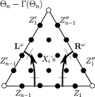
Figure 14. Quantum left and right matrices (compare Figure 12)

For a commutative algebra $\mathscr{A}$, in §1.6.2 we defined the classical matrices $\mathbf{M}^{\mathrm{left}}(X_{i}\text{'s})$, $\mathbf{M}^{\mathrm{right}}(X_{i}\text{'s})$, and $\mathbf{M}^{\mathrm{edge}}(Z_{j}\text{'s})$ in $\mathrm{SL}_{n}(\mathscr{A})$. When $\mathscr{A}=\mathbb{C}[X_{1}^{\pm 1/n},\dots,X_{N}^{\pm 1/n}]\cong\mathscr{T}_{n}^{1}$, we now use these matrices to define the primary objects of study.

Definition 28.

The quantum left matrix $\mathbf{L}^{\omega}$ in $\mathrm{M}_{n}(\mathscr{T}_{n}^{\omega})$ is defined by

$$\mathbf{L}^{\omega}=\mathbf{L}^{\omega}(X_{i},Z_{j},Z^{\prime}_{j}\text{'s})=\left[\mathbf{M}^{\mathrm{edge}}(Z_{j}\text{'s})\mathbf{M}^{\mathrm{left}}(X_{i}\text{'s})\mathbf{M}^{\mathrm{edge}}(Z^{\prime}_{j}\text{'s})\right]\quad\in\mathrm{M}_{n}\left(\mathscr{T}_{n}^{\omega}\right)$$

where we have applied the Weyl quantum ordering $[-]$ discussed in §2.3.1 to the product $\mathbf{M}^{\mathrm{edge}}(Z_{j}\text{'s})\mathbf{M}^{\mathrm{left}}(X_{i}\text{'s})\mathbf{M}^{\mathrm{edge}}(Z^{\prime}_{j}\text{'s})$ of classical matrices in $\mathrm{M}_{n}(\mathscr{T}_{n}^{1})$; see Figure 14.

Similarly, the quantum right matrix $\mathbf{R}^{\omega}$ in $\mathrm{M}_{n}(\mathscr{T}_{n}^{\omega})$ is defined by

$$\mathbf{R}^{\omega}=\mathbf{R}^{\omega}(X_{i},Z_{j},Z^{\prime\prime}_{j}\text{'s})=\left[\mathbf{M}^{\mathrm{edge}}(Z_{j}\text{'s})\mathbf{M}^{\mathrm{right}}(X_{i}\text{'s})\mathbf{M}^{\mathrm{edge}}(Z^{\prime\prime}_{j}\text{'s})\right]\quad\in\mathrm{M}_{n}\left(\mathscr{T}_{n}^{\omega}\right).$$

2.4. Main result

2.4.1. Quantum $\mathrm{SL}_{n}$ and its points

Let $\mathscr{T}$ be a, possibly non-commutative, algebra.

Definition 29.

We say that a $2\times 2$ matrix $\mathbf{M}=\left(\begin{smallmatrix}a&b\\ c&d\end{smallmatrix}\right)$ in $\mathrm{M}_{2}(\mathscr{T})$ is a $\mathscr{T}$-point of the quantum matrix algebra $\mathrm{M}_{2}^{q}$, denoted $\mathbf{M}\in\mathrm{M}_{2}^{q}(\mathscr{T})\subseteq\mathrm{M}_{2}(\mathscr{T})$, if

($$\ast ba=qab,\quad dc=qcd,\quad ca=qac,\quad db=qbd,\quad bc=cb,\quad da-ad=(q-q^{-1})bc\quad\in\mathscr{T}.$$)

We say that a matrix $\mathbf{M}\in\mathrm{M}_{2}(\mathscr{T})$ is a $\mathscr{T}$-point of the quantum special linear group $\mathrm{SL}_{2}^{q}$, denoted $\mathbf{M}\in\mathrm{SL}_{2}^{q}(\mathscr{T})\subseteq\mathrm{M}_{2}^{q}(\mathscr{T})\subseteq\mathrm{M}_{2}(\mathscr{T})$, if $\mathbf{M}\in\mathrm{M}_{2}^{q}(\mathscr{T})$ and the quantum determinant

$$\mathrm{Det}^{q}(\mathbf{M})\quad=da-qbc\quad=ad-q^{-1}bc\quad=1\quad\in\mathscr{T}.$$

These notions are also defined for $n\times n$ matrices, as follows.

Definition 30.

A matrix $\mathbf{M}\in\mathrm{M}_{n}(\mathscr{T})$ is a $\mathscr{T}$-point of the quantum matrix algebra $\mathrm{M}_{n}^{q}$, denoted $\mathbf{M}\in\mathrm{M}_{n}^{q}(\mathscr{T})\subseteq\mathrm{M}_{n}(\mathscr{T})$, if every $2\times 2$ submatrix of $\mathbf{M}$ is a $\mathscr{T}$-point of $\mathrm{M}_{2}^{q}$. That is,

$$\textbf{M}_{im}\textbf{M}_{ik}=q\textbf{M}_{ik}\textbf{M}_{im},\quad\quad\textbf{M}_{jm}\textbf{M}_{im}=q\textbf{M}_{im}\textbf{M}_{jm},$$

$$\textbf{M}_{im}\textbf{M}_{jk}=\textbf{M}_{jk}\textbf{M}_{im},\quad\quad\textbf{M}_{jm}\textbf{M}_{ik}-\textbf{M}_{ik}\textbf{M}_{jm}=(q-q^{-1})\textbf{M}_{im}\textbf{M}_{jk},$$

for all $i<j$ and $k<m$, where $1\leqslant i,j,k,m\leqslant n$.

There is a notion of the quantum determinant $\mathrm{Det}^{q}(\mathbf{M})\in\mathscr{T}$ of a $\mathscr{T}$-point $\mathbf{M}\in\mathrm{M}_{n}^{q}(\mathscr{T})$. A matrix $\mathbf{M}\in\mathrm{M}_{n}(\mathscr{T})$ is a $\mathscr{T}$-point of the quantum special linear group $\mathrm{SL}_{n}^{q}$, denoted $\mathbf{M}\in\mathrm{SL}_{n}^{q}(\mathscr{T})\subseteq\mathrm{M}_{n}^{q}(\mathscr{T})\subseteq\mathrm{M}_{n}(\mathscr{T})$, if both $\mathbf{M}\in\mathrm{M}_{n}^{q}(\mathscr{T})$ and $\mathrm{Det}^{q}(\mathbf{M})=1$.

The definitions satisfy the property that if a $\mathscr{T}$-point $\mathbf{M}\in\mathrm{M}_{n}^{q}(\mathscr{T})\subseteq\mathrm{M}_{n}(\mathscr{T})$ is a triangular matrix, then the diagonal entries $\mathbf{M}_{ii}\in\mathscr{T}$ commute, and $\mathrm{Det}^{q}(\mathbf{M})=\prod_{i}\mathbf{M}_{ii}\in\mathscr{T}$.

Remark 31.

The subsets $\mathrm{M}_{n}^{q}(\mathscr{T})\subseteq\mathrm{M}_{n}(\mathscr{T})$ and $\mathrm{SL}_{n}^{q}(\mathscr{T})\subseteq\mathrm{M}_{n}(\mathscr{T})$ are generally not closed under matrix multiplication (see, however, the sketch of proof below for a relaxed property).

2.4.2. Main result

Take $\mathscr{T}=\mathscr{T}_{n}^{\omega}=\mathscr{T}_{n}^{\omega}(\Theta_{n})$ to be the Fock-Goncharov quantum torus for the discrete $n$-triangle $\Theta_{n}$; see §2.2. For what follows, recall Definition 28.

Theorem 32.

The quantum left and right matrices

$$\mathbf{L}^{\omega},\quad\mathbf{R}^{\omega}\quad\in\mathrm{M}_{n}(\mathscr{T}_{n}^{\omega})$$

are $\mathscr{T}_{n}^{\omega}$-points of the quantum special linear group $\mathrm{SL}_{n}^{q}$. That is, $\mathbf{L}^{\omega},\mathbf{R}^{\omega}\in\mathrm{SL}_{n}^{q}(\mathscr{T}_{n}^{\omega})\subseteq\mathrm{M}_{n}(\mathscr{T}_{n}^{\omega})$.

The proof, provided in §3, uses a quantum version of Fock-Goncharov snakes (§1). Similar objects appeared independently in [CS20, SS17], motivated in part by [FG06a, GSV09].

Sketch of proof (see §3 for more details).

In the case $n=2$, this is an enjoyable calculation. When $n\geqslant 3$, the argument hinges on the following well-known fact: If $\mathscr{T}$ is an algebra with subalgebras $\mathscr{T}^{\prime},\mathscr{T}^{\prime\prime}\subseteq\mathscr{T}$ that commute in the sense that $a^{\prime}a^{\prime\prime}=a^{\prime\prime}a^{\prime}$ for all $a^{\prime}\in\mathscr{T}^{\prime}$ and $a^{\prime\prime}\in\mathscr{T}^{\prime\prime}$, and if $\mathbf{M}^{\prime}\in\mathrm{M}_{n}(\mathscr{T}^{\prime})\subseteq\mathrm{M}_{n}(\mathscr{T})$ and $\mathbf{M}^{\prime\prime}\in\mathrm{M}_{n}(\mathscr{T}^{\prime\prime})\subseteq\mathrm{M}_{n}(\mathscr{T})$ are $\mathscr{T}$-points of $\mathrm{SL}_{n}^{q}$, then the matrix product $\mathbf{M}^{\prime}\mathbf{M}^{\prime\prime}\in\mathrm{M}_{n}(\mathscr{T}^{\prime}\mathscr{T}^{\prime\prime})\subseteq\mathrm{M}_{n}(\mathscr{T})$ is also a $\mathscr{T}$-point of $\mathrm{SL}_{n}^{q}$.

Put $\mathbf{M}_{\mathrm{FG}}:=\mathbf{L}^{\omega}$, the Fock-Goncharov quantum left matrix, say. The proof will go the same for the quantum right matrix. The strategy is to see $\mathbf{M}_{\mathrm{FG}}\in\mathrm{M}_{n}(\mathscr{T}_{n}^{\omega})$ as the product of simpler matrices, over mutually-commuting subalgebras, that are themselves points of $\mathrm{SL}_{n}^{q}$.

More precisely, for a fixed sequence of adjacent snakes $\sigma^{\mathrm{bot}}=\sigma^{1},\sigma^{2},\dots,\sigma^{N}=\sigma^{\mathrm{top}}$ moving left across the triangle from the bottom edge to the top-left edge, we will define for each $i=1,\dots,N-1$ an auxiliary algebra $\mathscr{S}^{\omega}_{j_{i}}$ called a snake-move algebra, $j_{i}\in\{1,\dots,n-1\}$, corresponding to the adjacent snake pair $(\sigma^{i},\sigma^{i+1})$. As a technical step, there is a distinguished subalgebra $\mathscr{T}_{L}\subseteq\mathscr{T}_{n}^{\omega}$ satisfying $\mathbf{M}_{\mathrm{FG}}\in\mathrm{M}_{n}(\mathscr{T}_{L})\subseteq\mathrm{M}_{n}(\mathscr{T}_{n}^{\omega})$. We construct an algebra embedding $\mathscr{T}_{L}\hookrightarrow\bigotimes_{i}\mathscr{S}^{\omega}_{j_{i}}$. Through this embedding, we may view $\mathbf{M}_{\mathrm{FG}}\in\mathrm{M}_{n}(\mathscr{T}_{L})\subseteq~{}\mathrm{M}_{n}(\bigotimes_{i}\mathscr{S}^{\omega}_{j_{i}})$.

Following, we construct, for each $i$, a matrix $\mathbf{M}_{j_{i}}\in\mathrm{M}_{n}(\mathscr{S}^{\omega}_{j_{i}})\subseteq\mathrm{M}_{n}(\bigotimes_{i}\mathscr{S}^{\omega}_{j_{i}})$ with the property that $\mathbf{M}_{j_{i}}$ is a $\mathscr{S}^{\omega}_{j_{i}}$-point of $\mathrm{SL}_{n}^{q}$, in other words $\mathbf{M}_{j_{i}}\in\mathrm{SL}_{n}^{q}(\mathscr{S}^{\omega}_{j_{i}})\subseteq\mathrm{SL}_{n}^{q}(\bigotimes_{i}\mathscr{S}^{\omega}_{{j_{i}}})$. Since by definition the subalgebras $\mathscr{S}^{\omega}_{j_{i}},\mathscr{S}^{\omega}_{j_{i^{\prime}}}\subseteq\bigotimes_{i}\mathscr{S}^{\omega}_{j_{i}}$ commute if $i\neq i^{\prime}$, as they constitute different tensor factors of $\bigotimes_{i}\mathscr{S}^{\omega}_{j_{i}}$, it follows from the essential fact mentioned above that $\mathbf{M}:=\mathbf{M}_{j_{1}}\mathbf{M}_{j_{2}}\cdots\mathbf{M}_{j_{N-1}}\in\mathrm{M}_{n}(\bigotimes_{i}\mathscr{S}^{\omega}_{j_{i}})$ is a $(\bigotimes_{i}\mathscr{S}^{\omega}_{j_{i}})$-point of $\mathrm{SL}_{n}^{q}$, in other words $\mathbf{M}\in~{}\mathrm{SL}_{n}^{q}(\bigotimes_{i}\mathscr{S}^{\omega}_{j_{i}})$.

Now, since this matrix product $\mathbf{M}$, as well as the quantum left matrix $\mathbf{M}_{\mathrm{FG}}$, are being viewed as elements of $\mathrm{M}_{n}(\bigotimes_{i}\mathscr{S}^{\omega}_{j_{i}})$, it makes sense to ask whether $\mathbf{M}_{\mathrm{FG}}\overset{?}{=}\mathbf{M}\in\mathrm{M}_{n}(\bigotimes_{i}\mathscr{S}^{\omega}_{j_{i}})$. Indeed, this turns out to be true, implying that $\mathbf{M}_{\mathrm{FG}}\in\mathrm{SL}_{n}^{q}(\bigotimes_{i}\mathscr{S}^{\omega}_{j_{i}})$. Since, as we know, $\mathbf{M}_{\mathrm{FG}}\in\mathrm{M}_{n}(\mathscr{T}_{L})\subseteq\mathrm{M}_{n}(\bigotimes_{i}\mathscr{S}^{\omega}_{j_{i}})$, we conclude that $\mathbf{M}_{\mathrm{FG}}$ is in $\mathrm{SL}_{n}^{q}(\mathscr{T}_{L})\subseteq\mathrm{SL}_{n}^{q}(\mathscr{T}_{n}^{\omega})$. ∎

2.5. Example

Consider the case $n=4$; see Figure 15. On the right hand side we show the commutation relations in the quantum torus $\mathscr{T}_{4}^{\omega}$, recalling Figure 13, but viewed in $\Theta_{n-1}$ (compare Figures 9 and 10). For instance, some sample commutation relations are:

$$X_{3}Z^{\prime\prime}_{2}=q^{2}X_{3}Z^{\prime\prime}_{2},\quad\quad X_{3}X_{1}=q^{-2}X_{1}X_{3},\quad\quad Z_{3}Z_{2}=qZ_{2}Z_{3},\quad\quad Z_{3}Z^{\prime}_{3}=q^{2}Z^{\prime}_{3}Z_{3}.$$

(a) Left and right matrices

(b) Quiver

Figure 15. Quantum matrices and quantum torus ($n=4$)

Then, the quantum left and right matrices $\mathbf{L}^{\omega}$ and $\mathbf{R}^{\omega}$ are computed as

$$\begin{split}\mathbf{L}^{\omega}=&\Bigg{[}Z_{1}^{-\frac{1}{4}}Z_{2}^{-\frac{2}{4}}Z_{3}^{-\frac{3}{4}}\left(\begin{smallmatrix}Z_{1}Z_{2}Z_{3}&&&\\ &Z_{2}Z_{3}&&\\ &&Z_{3}&\\ &&&1\end{smallmatrix}\right)\left(\begin{smallmatrix}1&1&&\\ &1&&\\ &&1&\\ &&&1\end{smallmatrix}\right)X_{1}^{-\frac{1}{4}}\left(\begin{smallmatrix}X_{1}&&&\\ &1&1&\\ &&1&\\ &&&1\end{smallmatrix}\right)X_{2}^{-\frac{2}{4}}\left(\begin{smallmatrix}X_{2}&&&\\ &X_{2}&&\\ &&1&1\\ &&&1\end{smallmatrix}\right)\\ &\left(\begin{smallmatrix}1&1&&\\ &1&&\\ &&1&\\ &&&1\end{smallmatrix}\right)X_{3}^{-\frac{1}{4}}\left(\begin{smallmatrix}X_{3}&&&\\ &1&1&\\ &&1&\\ &&&1\end{smallmatrix}\right)\left(\begin{smallmatrix}1&1&&\\ &1&&\\ &&1&\\ &&&1\end{smallmatrix}\right)Z_{1}^{\prime-\frac{1}{4}}Z_{2}^{\prime-\frac{2}{4}}Z_{3}^{\prime-\frac{3}{4}}\left(\begin{smallmatrix}Z^{\prime}_{1}Z^{\prime}_{2}Z^{\prime}_{3}&&&\\ &Z^{\prime}_{2}Z^{\prime}_{3}&&\\ &&Z^{\prime}_{3}&\\ &&&1\end{smallmatrix}\right)\Bigg{]};\end{split}$$

and

$$\begin{split}\mathbf{R}^{\omega}=&\Bigg{[}Z_{1}^{-\frac{1}{4}}Z_{2}^{-\frac{2}{4}}Z_{3}^{-\frac{3}{4}}\left(\begin{smallmatrix}Z_{1}Z_{2}Z_{3}&&&\\ &Z_{2}Z_{3}&&\\ &&Z_{3}&\\ &&&1\end{smallmatrix}\right)\left(\begin{smallmatrix}1&&&\\ &1&&\\ &&1&\\ &&1&1\end{smallmatrix}\right)X_{2}^{+\frac{1}{4}}\left(\begin{smallmatrix}1&&&\\ &1&&\\ &1&1&\\ &&&X_{2}^{-1}\end{smallmatrix}\right)X_{1}^{+\frac{2}{4}}\left(\begin{smallmatrix}1&&&\\ 1&1&&\\ &&X_{1}^{-1}&\\ &&&X_{1}^{-1}\end{smallmatrix}\right)\\ &\left(\begin{smallmatrix}1&&&\\ &1&&\\ &&1&\\ &&1&1\end{smallmatrix}\right)X_{3}^{+\frac{1}{4}}\left(\begin{smallmatrix}1&&&\\ &1&&\\ &1&1&\\ &&&X_{3}^{-1}\end{smallmatrix}\right)\left(\begin{smallmatrix}1&&&\\ &1&&\\ &&1&\\ &&1&1\end{smallmatrix}\right)Z_{1}^{\prime\prime-\frac{1}{4}}Z_{2}^{\prime\prime-\frac{2}{4}}Z_{3}^{\prime\prime-\frac{3}{4}}\left(\begin{smallmatrix}Z^{\prime\prime}_{1}Z^{\prime\prime}_{2}Z_{3}^{\prime\prime}&&&\\ &Z^{\prime\prime}_{2}Z^{\prime\prime}_{3}&&\\ &&Z^{\prime\prime}_{3}&\\ &&&1\end{smallmatrix}\right)\Bigg{]}.\end{split}$$

The theorem says that these two matrices are elements of $\mathrm{SL}_{4}^{q}(\mathscr{T}_{4}^{\omega})$. For instance, the entries $a,b,c,d$ of the $2\times 2$ submatrix (arranged as a $4\times 1$ matrix) of $\mathbf{L}^{\omega}$

$$\begin{split}\left(\begin{smallmatrix}a\\ b\\ c\\ d\end{smallmatrix}\right)=\left(\begin{smallmatrix}\mathbf{L}^{\omega}_{13}\\ \mathbf{L}^{\omega}_{14}\\ \mathbf{L}^{\omega}_{23}\\ \mathbf{L}^{\omega}_{24}\end{smallmatrix}\right)=\left(\begin{smallmatrix}[Z_{3}^{\frac{1}{4}}Z_{2}^{\frac{2}{4}}Z_{1}^{\frac{3}{4}}Z_{3}^{\prime\frac{1}{4}}Z_{2}^{\prime-\frac{2}{4}}Z_{1}^{\prime-\frac{1}{4}}X_{1}^{-\frac{1}{4}}X_{2}^{-\frac{2}{4}}X_{3}^{-\frac{1}{4}}]+[Z_{3}^{\frac{1}{4}}Z_{2}^{\frac{2}{4}}Z_{1}^{\frac{3}{4}}Z_{3}^{\prime\frac{1}{4}}Z_{2}^{\prime-\frac{2}{4}}Z_{1}^{\prime-\frac{1}{4}}X_{1}^{-\frac{1}{4}}X_{2}^{\frac{2}{4}}X_{3}^{-\frac{1}{4}}]+\\ +[Z_{3}^{\frac{1}{4}}Z_{2}^{\frac{2}{4}}Z_{1}^{\frac{3}{4}}Z_{3}^{\prime\frac{1}{4}}Z_{2}^{\prime-\frac{2}{4}}Z_{1}^{\prime-\frac{1}{4}}X_{1}^{\frac{3}{4}}X_{2}^{\frac{2}{4}}X_{3}^{-\frac{1}{4}}]\\ [Z_{3}^{\frac{1}{4}}Z_{2}^{\frac{2}{4}}Z_{1}^{\frac{3}{4}}Z_{3}^{\prime-\frac{3}{4}}Z_{2}^{\prime-\frac{2}{4}}Z_{1}^{\prime-\frac{1}{4}}X_{1}^{-\frac{1}{4}}X_{2}^{-\frac{2}{4}}X_{3}^{-\frac{1}{4}}]\\ [Z_{3}^{\frac{1}{4}}Z_{2}^{\frac{2}{4}}Z_{1}^{-\frac{1}{4}}Z_{3}^{\prime\frac{1}{4}}Z_{2}^{\prime-\frac{2}{4}}Z_{1}^{\prime-\frac{1}{4}}X_{1}^{-\frac{1}{4}}X_{2}^{-\frac{2}{4}}X_{3}^{-\frac{1}{4}}]+[Z_{3}^{\frac{1}{4}}Z_{2}^{\frac{2}{4}}Z_{1}^{-\frac{1}{4}}Z_{3}^{\prime\frac{1}{4}}Z_{2}^{\prime-\frac{2}{4}}Z_{1}^{\prime-\frac{1}{4}}X_{1}^{-\frac{1}{4}}X_{2}^{\frac{2}{4}}X_{3}^{-\frac{1}{4}}]\\ [Z_{3}^{\frac{1}{4}}Z_{2}^{\frac{2}{4}}Z_{1}^{-\frac{1}{4}}Z_{3}^{\prime-\frac{3}{4}}Z_{2}^{\prime-\frac{2}{4}}Z_{1}^{\prime-\frac{1}{4}}X_{1}^{-\frac{1}{4}}X_{2}^{-\frac{2}{4}}X_{3}^{-\frac{1}{4}}]\end{smallmatrix}\right)\end{split}$$

satisfy Equation ($\ast$ ‣ 29). For a computer demonstration of this, see [Dou21, Appendix A]. We also verify in that appendix that Equation ($\ast$ ‣ 29) is satisfied by the entries $a,b,c,d$ of the $2\times 2$ submatrix (arranged as a $4\times 1$ matrix) of $\mathbf{R}^{\omega}$

$$\begin{split}\left(\begin{smallmatrix}a\\ b\\ c\\ d\end{smallmatrix}\right)\!=\!\left(\begin{smallmatrix}\mathbf{R}^{\omega}_{31}\\ \mathbf{R}^{\omega}_{32}\\ \mathbf{R}^{\omega}_{41}\\ \mathbf{R}^{\omega}_{42}\end{smallmatrix}\right)\!=\!\left(\begin{smallmatrix}[Z_{3}^{\frac{1}{4}}Z_{2}^{-\frac{1}{2}}Z_{1}^{-\frac{1}{4}}X_{2}^{\frac{1}{4}}X_{1}^{\frac{1}{2}}X_{3}^{\frac{1}{4}}Z_{3}^{\prime\prime\frac{1}{4}}Z_{2}^{\prime\prime\frac{1}{2}}Z_{1}^{\prime\prime\frac{3}{4}}]\\ [Z_{3}^{\frac{1}{4}}Z_{2}^{-\frac{1}{2}}Z_{1}^{-\frac{1}{4}}X_{2}^{\frac{1}{4}}X_{1}^{-\frac{1}{2}}X_{3}^{\frac{1}{4}}Z_{3}^{\prime\prime\frac{1}{4}}Z_{2}^{\prime\prime\frac{1}{2}}Z_{1}^{\prime\prime-\frac{1}{4}}]+[Z_{3}^{\frac{1}{4}}Z_{2}^{-\frac{1}{2}}Z_{1}^{-\frac{1}{4}}X_{2}^{\frac{1}{4}}X_{1}^{\frac{1}{2}}X_{3}^{\frac{1}{4}}Z_{3}^{\prime\prime\frac{1}{4}}Z_{2}^{\prime\prime\frac{1}{2}}Z_{1}^{\prime\prime-\frac{1}{4}}]\\ [Z_{3}^{-\frac{3}{4}}Z_{2}^{-\frac{1}{2}}Z_{1}^{-\frac{1}{4}}X_{2}^{\frac{1}{4}}X_{1}^{\frac{1}{2}}X_{3}^{\frac{1}{4}}Z_{3}^{\prime\prime\frac{1}{4}}Z_{2}^{\prime\prime\frac{1}{2}}Z_{1}^{\prime\prime\frac{3}{4}}]\\ [Z_{3}^{-\frac{3}{4}}Z_{2}^{-\frac{1}{2}}Z_{1}^{-\frac{1}{4}}X_{2}^{-\frac{3}{4}}X_{1}^{-\frac{1}{2}}X_{3}^{\frac{1}{4}}Z_{3}^{\prime\prime\frac{1}{4}}Z_{2}^{\prime\prime\frac{1}{2}}Z_{1}^{\prime\prime-\frac{1}{4}}]+[Z_{3}^{-\frac{3}{4}}Z_{2}^{-\frac{1}{2}}Z_{1}^{-\frac{1}{4}}X_{2}^{\frac{1}{4}}X_{1}^{-\frac{1}{2}}X_{3}^{\frac{1}{4}}Z_{3}^{\prime\prime\frac{1}{4}}Z_{2}^{\prime\prime\frac{1}{2}}Z_{1}^{\prime\prime-\frac{1}{4}}]+\\ +[Z_{3}^{-\frac{3}{4}}Z_{2}^{-\frac{1}{2}}Z_{1}^{-\frac{1}{4}}X_{2}^{\frac{1}{4}}X_{1}^{\frac{1}{2}}X_{3}^{\frac{1}{4}}Z_{3}^{\prime\prime\frac{1}{4}}Z_{2}^{\prime\prime\frac{1}{2}}Z_{1}^{\prime\prime-\frac{1}{4}}]\end{smallmatrix}\right).\end{split}$$

Remark 33.

Puzzlingly, in order for these matrices to satisfy the relations required just to be in $\mathrm{M}_{n}^{q}(\mathscr{T}_{n}^{\omega})$ (let alone $\mathrm{SL}_{n}^{q}(\mathscr{T}_{n}^{\omega})$), they have to be normalized by “dividing out” their determinants. For example, the above matrix $\mathbf{L}^{\omega}$ for $n=4$ would not satisfy the $q$-commutation relations required to be a point of $\mathrm{M}_{4}^{q}$ if we had not included the normalizing term $Z_{1}^{-\frac{1}{4}}Z_{2}^{-\frac{2}{4}}Z_{3}^{-\frac{3}{4}}X_{1}^{-\frac{1}{4}}X_{2}^{-\frac{2}{4}}X_{3}^{-\frac{1}{4}}Z_{1}^{\prime-\frac{1}{4}}Z_{2}^{\prime-\frac{2}{4}}Z_{3}^{\prime-\frac{3}{4}}$, as there would be a $1$ in the bottom corner.

3. Quantum snakes: proof of Theorem 32

Above, we gave a sketch of the proof. We now fill in the details. Our emphasis will be on the left matrix $\mathbf{L}^{\omega}$. The proof for the right matrix $\mathbf{R}^{\omega}$ is similar, as we will discuss in §3.5.

Fix a sequence $\sigma^{\mathrm{bot}}=\sigma^{1},\sigma^{2},\dots,\sigma^{N}=\sigma^{\mathrm{top}}$ of adjacent snakes, as in the left setting; see §1.6.1. The proof is valid for any choice of snake sequence, but we always demonstrate it in figures and examples for our preferred snake sequence; see Figure 11. Note that the example quantum matrices in §2.5 were presented using this preferred sequence.

3.1. Snake-move quantum tori

Definition 34.

For $j=1,\dots,n-1$, the $j$-th snake-move quantum torus $\mathscr{S}^{\omega}_{j}=\mathscr{T}(\mathbf{P}_{j})$ is the quantum torus with Poisson matrix $\mathbf{P}_{j}$ defined by the quiver shown in Figure 16 when $j=2,\dots,n-1$, and in Figure 17 when $j=1$. As usual, there is one generator per edge of the quiver, solid arrows carry a weight $2$, and dotted arrows carry a weight $1$; compare §2.2.

Figure 16. Diamond snake-move algebra ($j=2,\dots,n-1$)

Figure 17. Tail snake-move algebra ($j=1$)

Remark 35.

The quiver of Figure 17 for the tail-move quantum torus is divided into a bottom and top side. Similarly, the quiver of Figure 16 for a diamond-move quantum torus has a bottom and top side, connected by a diagonal. Conceptually speaking, as illustrated in the figures, we think of the bottom side (with un-primed generators $z_{j}$) as the top “snake-skin” $\sigma_{1/2}$ of a snake $\sigma$ that has been “split in half down its length”. Similarly, we think of the top side (with primed generators $z_{j}^{\prime}$) as the bottom snake-skin $\sigma^{\prime}_{1/2}$ of a split snake $\sigma^{\prime}$. Compare Figures 3 and 8, illustrating snakes in the classical setting.

This snake splitting can be seen more clearly in the quantum snake sweep (see §3.3 and Figure 18 below) determined by the sequence of adjacent snakes $\sigma^{\mathrm{bot}}=\sigma^{1},\sigma^{2},\dots,\sigma^{N}=\sigma^{\mathrm{top}}$, where each snake $\sigma^{i}$ is split in half, so that each half’s snake-skin forms a side in one of two adjacent snake-move quantum tori. In the figure, the other halves of the bottom-most and top-most quantum snakes (colored grey) can be thought of as either living in other triangles or not existing at all. Prior to splitting a snake $\sigma$ in half, the snake consists of $n-1$ “vertebrae” connecting the $n$ snake-vertices $\sigma_{k}\in\Theta_{n-1}$. Upon splitting the snake, the $j$-th vertebra splits into two generators $z_{j}$ and $z_{j}^{\prime}$ living in adjacent snake-move quantum tori.

3.2. Quantum snake-move matrices

We turn to the key observation for the proof.

Proposition 36.

For $j=1,\dots,n-1$, the $j$-th quantum snake-move matrix

$$\mathbf{M}_{j}:=\left[\left(\prod_{k=1}^{n-1}\mathbf{S}^{\mathrm{edge}}_{k}(z_{k})\right)\mathbf{S}^{\mathrm{left}}_{j}(x_{j-1})\left(\prod_{k=1}^{n-1}\mathbf{S}^{\mathrm{edge}}_{k}(z^{\prime}_{k})\right)\right]\quad\in\mathrm{M}_{n}(\mathscr{S}^{\omega}_{j})$$

is a $\mathscr{S}^{\omega}_{j}$-point of the quantum special linear group $\mathrm{SL}_{n}^{q}$. That is, $\mathbf{M}_{j}\in\mathrm{SL}_{n}^{q}(\mathscr{S}^{\omega}_{j})\subseteq\mathrm{M}_{n}(\mathscr{S}^{\omega}_{j})$.

Note the use of the Weyl quantum ordering; see §2.1.3. Here, the matrices $\mathbf{S}_{j}^{\mathrm{edge}}(z)$ and $\mathbf{S}_{j}^{\mathrm{left}}(x)$ for $z,x$ in the commutative algebra $\mathscr{S}_{j}^{1}$ are defined as in §1.4.1; see also §2.3.1-2.3.2. Note when $j=1$, the matrix $\mathbf{S}^{\mathrm{left}}_{1}(x_{0})=\mathbf{S}^{\mathrm{left}}_{1}$ is well-defined, despite $x_{0}$ not being defined.

Proof.

This is a direct calculation, checking that the entries of the matrix $\mathbf{M}_{j}$ satisfy the relations of the dual quantum group $\mathrm{SL}_{n}^{q}$ in the $j$-th snake-move quantum torus $\mathscr{S}^{\omega}_{j}$. ∎

For example, in the case $n=4$, $j=3$, the lemma says that the matrix

$$\mathbf{M}_{3}=\left[z_{1}^{-\frac{1}{4}}z_{2}^{-\frac{2}{4}}z_{3}^{-\frac{3}{4}}\left(\begin{smallmatrix}z_{1}z_{2}z_{3}&&&\\ &z_{2}z_{3}&&\\ &&z_{3}&\\ &&&1\end{smallmatrix}\right)x_{2}^{-\frac{2}{4}}\left(\begin{smallmatrix}x_{2}&&&\\ &x_{2}&&\\ &&1&1\\ &&&1\end{smallmatrix}\right)z_{1}^{\prime-\frac{1}{4}}z_{2}^{\prime-\frac{2}{4}}z_{3}^{\prime-\frac{3}{4}}\left(\begin{smallmatrix}z^{\prime}_{1}z^{\prime}_{2}z^{\prime}_{3}&&&\\ &z^{\prime}_{2}z^{\prime}_{3}&&\\ &&z^{\prime}_{3}&\\ &&&1\end{smallmatrix}\right)\right]$$

is in $\mathrm{SL}_{4}^{q}(\mathscr{S}^{\omega}_{3})$. The Weyl ordering is needed to satisfy the quantum determinant relation.

3.3. Technical step: embedding a distinguished subalgebra $\mathscr{T}_{L}$ of $\mathscr{T}_{n}^{\omega}$ into a tensor product of snake-move quantum tori

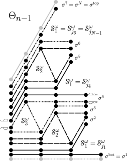
Figure 18. Quantum snake sweep ($n=4$); compare Figure 11(a)

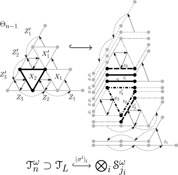
Figure 19. Embedding $\mathscr{T}_{L}$ in the tensor product of snake-move quantum tori

For the snake-sequence $(\sigma^{i})_{i=1,\dots,N}$, to each pair $(\sigma^{i},\sigma^{i+1})$ of adjacent snakes we associate a snake-move quantum torus $\mathscr{S}^{\omega}_{j_{i}}$, recalling Remark 35 and Figure 18. Recall the Fock-Goncharov quantum torus $\mathscr{T}_{n}^{\omega}$; see Figures 13 and 15.

We now take a technical step. Define $\mathscr{T}_{L}\subseteq\mathscr{T}_{n}^{\omega}$ (“$L$” for “Left”) to be the subalgebra generated by all the generators (and their inverses) of $\mathscr{T}_{n}^{\omega}$ except for $Z_{1}^{\prime\prime\pm 1/n},\dots,Z_{n-1}^{\prime\prime\pm 1/n}$; see Figures 14 and 15. We claim that the snake-sequence $(\sigma^{i})_{i}$ (Figure 11) induces an embedding

$$\mathscr{T}_{n}^{\omega}\supseteq\mathscr{T}_{L}\overset{(\sigma^{i})_{i}}{\longhookrightarrow}\bigotimes_{i=1}^{N-1}\mathscr{S}^{\omega}_{j_{i}}$$

of algebras, realizing $\mathscr{T}_{L}\subseteq\mathscr{T}_{n}^{\omega}$ as a subalgebra of the tensor product of the snake-move quantum tori $\mathscr{S}^{\omega}_{j_{i}}$ (tensored from left to right) associated to the adjacent snake pairs $(\sigma^{i},\sigma^{i+1})$.

We explain the embedding through an example, in the case $n=4$; see Figure 19 (compare Figure 18). There, the generator $X_{2}$ (emphasized in the figure), for instance, is mapped to

$$X_{2}\mapsto 1\otimes z^{\prime}_{2}\otimes z_{2}x_{2}z^{\prime}_{2}\otimes z_{2}z^{\prime}_{2}\otimes z_{2}\otimes 1\quad\quad\quad\in\mathscr{S}^{\omega}_{1}\otimes\mathscr{S}^{\omega}_{2}\otimes\mathscr{S}^{\omega}_{3}\otimes\mathscr{S}^{\omega}_{1}\otimes\mathscr{S}^{\omega}_{2}\otimes\mathscr{S}^{\omega}_{1}.$$

Similarly, the generators $Z_{1}$ and $Z^{\prime}_{3}$, say, are mapped to

$$Z_{1}\mapsto z_{1}\otimes 1\otimes 1\otimes 1\otimes 1\otimes 1,\quad\quad Z^{\prime}_{3}\mapsto 1\otimes 1\otimes z^{\prime}_{3}\otimes z_{3}z^{\prime}_{3}\otimes z_{3}z^{\prime}_{3}\otimes z_{3}z^{\prime}_{3}.$$

The remaining generators $Z_{2},Z_{3},X_{1},X_{1}^{\prime},Z_{2}^{\prime},Z_{1}^{\prime}$ are mapped to

$$Z_{2} \mapsto z_{2}z_{2}^{\prime}\otimes z_{2}\otimes 1\otimes 1\otimes 1\otimes 1, Z_{3} \mapsto z_{3}z_{3}^{\prime}\otimes z_{3}z_{3}^{\prime}\otimes z_{3}\otimes 1\otimes 1\otimes 1,$$

$$X_{1} \mapsto z_{1}^{\prime}\otimes z_{1}x_{1}z_{1}^{\prime}\otimes z_{1}z_{1}^{\prime}\otimes z_{1}\otimes 1\otimes 1, X_{1}^{\prime} \mapsto 1\otimes 1\otimes 1\otimes z_{1}^{\prime}\otimes z_{1}x_{1}z_{1}^{\prime}\otimes z_{1},$$

$$Z_{2}^{\prime} \mapsto 1\otimes 1\otimes 1\otimes 1\otimes z_{2}^{\prime}\otimes z_{2}z_{2}^{\prime} Z_{1}^{\prime} \mapsto 1\otimes 1\otimes 1\otimes 1\otimes 1\otimes z_{1}^{\prime}.$$

Note that the monomials (for instance, $z_{2}x_{2}z^{\prime}_{2}$ or $z_{2}z_{2}^{\prime}$) appearing in the $i$-th tensor factor of the image of a generator $X$ or $Z$ of the subalgebra $\mathscr{T}_{L}$ under this mapping consist of mutually commuting generators $x$’s and/or $z$’s of the $i$-th snake-move quantum torus $\mathscr{S}_{j_{i}}^{\omega}$, so the order in which they are written is irrelevant. It is clear from Figure 19 that these images satisfy the relations of $\mathscr{T}_{L}$. In particular, the “interior” dotted arrows lying at each interface between two snake-move quantum tori “cancel each other out”; note that, in Figure 19, we have omitted drawing some of these dotted arrows. We gather that the mapping is well-defined and is an algebra homomorphism. Injectivity follows from the property that every generator (that is, quiver edge) appearing on the right side of Figure 19 corresponds to a unique generator on the left side. Lastly, we technically should have defined the map on the formal $n$-roots of the generators of $\mathscr{T}_{L}$. This is done in the obvious way, for instance,

$$X_{2}^{1/4}\mapsto 1\otimes z^{\prime 1/4}_{2}\otimes z_{2}^{1/4}x_{2}^{1/4}z^{\prime 1/4}_{2}\otimes z_{2}^{1/4}z^{\prime 1/4}_{2}\otimes z_{2}^{1/4}\otimes 1\quad\in\mathscr{S}^{\omega}_{1}\otimes\mathscr{S}^{\omega}_{2}\otimes\mathscr{S}^{\omega}_{3}\otimes\mathscr{S}^{\omega}_{1}\otimes\mathscr{S}^{\omega}_{2}\otimes\mathscr{S}^{\omega}_{1}.$$

Remark 37.

The definition of this embedding is reminiscent of Propositions 21 and 22, where the triangle and edge invariants $X_{i}$ and $Z_{j}$ are decomposed as “products” of shears.

3.4. Finishing the proof

Comparing to the sketch of proof given in §2.4.2, we gather:

• $\mathbf{M}_{\mathrm{FG}}:=\mathbf{L}^{\omega}\quad\in\mathrm{M}_{n}(\mathscr{T}_{L})\quad\subseteq\mathrm{M}_{n}\left(\bigotimes_{i=1}^{N-1}\mathscr{S}^{\omega}_{j_{i}}\right)$;

• $\mathbf{M}:=\mathbf{M}_{j_{1}}\mathbf{M}_{j_{2}}\cdots\mathbf{M}_{j_{N-1}}\quad\in\mathrm{SL}_{n}^{q}\left(\bigotimes_{i=1}^{N-1}\mathscr{S}^{\omega}_{j_{i}}\right)\quad\subseteq\mathrm{M}_{n}\left(\bigotimes_{i=1}^{N-1}\mathscr{S}^{\omega}_{j_{i}}\right)$.

To finish the proof, it remains to show

($$\ast \mathbf{M}_{\mathrm{FG}}\overset{?}{=}\mathbf{M}=\mathbf{M}_{j_{1}}\mathbf{M}_{j_{2}}\cdots\mathbf{M}_{j_{N-1}}\quad\in\mathrm{M}_{n}\left(\bigotimes_{i=1}^{N-1}\mathscr{S}^{\omega}_{j_{i}}\right).$$)

This is straightforward, albeit a bit tricky to write down due to the triangular combinatorics. We first sketch the argument. The strategy is to commute the many variables (as in the right hand side of Figure 19) appearing on the right hand side $\mathbf{M}=\prod_{i}\mathbf{M}_{j_{i}}$ (defined via Proposition 36) of Equation ($\ast$ ‣ 3.4), until $\mathbf{M}$ has been put into the form of the left hand side $\mathbf{M}_{\mathrm{FG}}$ (defined via Definition 28 followed by applying the embedding $\mathscr{T}_{L}\hookrightarrow\bigotimes_{i}\mathscr{S}^{\omega}_{j_{i}}$ of §3.3). This is accomplished by applying the following two facts, whose proofs are immediate.

Lemma 38.

1. If $\widetilde{\mathbf{M}}_{1},\widetilde{\mathbf{M}}_{2},\dots,\widetilde{\mathbf{M}}_{N-1}$ are matrices with coefficients in $q=w=1$ specializations $\mathscr{T}^{1}_{i}$ of quantum tori $\mathscr{T}^{\omega}_{1},\mathscr{T}^{\omega}_{2},\dots,\mathscr{T}^{\omega}_{N-1}$, viewed as factors in $\mathscr{T}^{\omega}_{1}\otimes\mathscr{T}^{\omega}_{2}\otimes\cdots\otimes\mathscr{T}^{\omega}_{N-1}$, then

   $$\left[\widetilde{\mathbf{M}}_{1}\right]\left[\widetilde{\mathbf{M}}_{2}\right]\cdots\left[\widetilde{\mathbf{M}}_{N-1}\right]=\left[\widetilde{\mathbf{M}}_{1}\widetilde{\mathbf{M}}_{2}\cdots\widetilde{\mathbf{M}}_{N-1}\right]\quad\in\mathrm{M}_{n}\left(\mathscr{T}^{\omega}_{1}\otimes\mathscr{T}^{\omega}_{2}\otimes\cdots\otimes\mathscr{T}^{\omega}_{N-1}\right).$$

2. For commuting variables $z$ and $x$, the matrices $\mathbf{S}^{\mathrm{edge}}_{k}(z)$ and $\mathbf{S}^{\mathrm{left}}_{j}(x)$, as in §1.4.1 and Proposition 36, satisfy

   $$\mathbf{S}^{\mathrm{edge}}_{k}(z)\mathbf{S}^{\mathrm{left}}_{j}(x)=\mathbf{S}^{\mathrm{left}}_{j}(x)\mathbf{S}^{\mathrm{edge}}_{k}(z)\quad\text{ if and only if }\quad k\neq j.$$

Proof of Theorem 32.

By part (1) of Lemma 38, it suffices to establish Equation ($\ast$ ‣ 3.4) when $q=\omega=1$, in which case we do not need to worry about the Weyl quantum ordering.

It is helpful to introduce a simplifying notation. For coordinates $z_{k}^{(i)},x^{(i)}_{j},z^{\prime(i)}_{k}\in\mathscr{S}_{j_{i}}^{1}$, put

$$\mathbf{Z}_{k}^{(i)}:=\mathbf{S}_{k}^{\mathrm{edge}}(z_{k}^{(i)}),\quad\quad\mathbf{X}_{j}^{(i)}:=\mathbf{S}^{\mathrm{left}}_{j+1}(x_{j}^{(i)}),\quad\quad\mathbf{Z}_{k}^{\prime(i)}:=\mathbf{S}_{k}^{\mathrm{edge}}(z^{\prime(i)}_{k})\quad\quad\in\mathrm{M}_{n}(\mathscr{S}^{1}_{j_{i}}).$$

In this new notation, the matrices $\mathbf{M}_{j_{i}}\in\mathrm{M}_{n}(\mathscr{S}^{1}_{j_{i}})$ of Proposition 36 can be expressed by

$$\mathbf{M}_{j_{i}}=\left(\prod_{k=1}^{n-1}\mathbf{Z}_{k}^{(i)}\right)\mathbf{X}^{(i)}_{j_{i}-1}\left(\prod_{k=1}^{n-1}\mathbf{Z}_{k}^{\prime(i)}\right)\quad\quad\in\mathrm{M}_{n}(\mathscr{S}^{1}_{j_{i}})$$

and part (2) of Lemma 38 now reads, for any $i_{1},i_{2}\in\{1,2,\dots,N-1\}$,

($$\dagger \mathbf{Z}^{(i_{1})}_{k}\mathbf{X}_{j}^{(i_{2})}=\mathbf{X}_{j}^{(i_{2})}\mathbf{Z}^{(i_{1})}_{k}\in\mathrm{M}_{n}\left(\bigotimes_{i=1}^{N-1}\mathscr{S}^{1}_{j_{i}}\right)\quad\text{ if and only if }\quad k\neq j+1\quad(\text{similarly for }\mathbf{Z}\to\mathbf{Z}^{\prime}).$$)

Example: n=2. In this case, $N=2$, we have $\mathscr{S}_{j_{1}}^{1}=\mathscr{S}_{1}^{1}\cong\mathscr{T}_{L}\subseteq\mathscr{T}_{n}^{1}$, and the embedding $\mathscr{T}_{L}\overset{\sim}{\hookrightarrow}\mathscr{S}_{1}^{1}$ is the identity, $Z_{1}\mapsto z_{1}^{(1)}$, $Z_{1}^{\prime}\mapsto z_{1}^{\prime(1)}$. Equation ($\ast$ ‣ 3.4) is also trivial, reading

$$\begin{split}\mathbf{M}=\mathbf{M}_{1}=\mathbf{Z}_{1}^{(1)}\mathbf{X}_{0}^{(1)}\mathbf{Z}_{1}^{\prime(1)}&=z_{1}^{(1)\frac{-1}{2}}\left(\begin{smallmatrix}z_{1}^{(1)}&0\\ 0&1\end{smallmatrix}\right)\left(\begin{smallmatrix}1&1\\ 0&1\end{smallmatrix}\right)z_{1}^{\prime(1)\frac{-1}{2}}\left(\begin{smallmatrix}z^{\prime(1)}_{1}&0\\ 0&1\end{smallmatrix}\right)\\ &=Z_{1}^{-\frac{1}{2}}\left(\begin{smallmatrix}Z_{1}&0\\ 0&1\end{smallmatrix}\right)\left(\begin{smallmatrix}1&1\\ 0&1\end{smallmatrix}\right)Z_{1}^{\prime-\frac{1}{2}}\left(\begin{smallmatrix}Z^{\prime}_{1}&0\\ 0&1\end{smallmatrix}\right)=\mathbf{S}^{\mathrm{edge}}_{1}(Z_{1})\mathbf{S}^{\mathrm{left}}_{1}\mathbf{S}^{\mathrm{edge}}_{1}(Z_{1}^{\prime})=\mathbf{M}_{\mathrm{FG}}.\end{split}$$

Example: n=3. Here $N=4$, the subalgebra $\mathscr{T}_{L}$ has coordinates $Z_{1},Z_{2},X_{1},Z_{1}^{\prime},Z_{2}^{\prime}$, and the embedding $\mathscr{T}_{L}\hookrightarrow\mathscr{S}^{1}_{1}\otimes\mathscr{S}^{1}_{2}\otimes\mathscr{S}^{1}_{1}$ is defined by (compare the $n=4$ case, Figure 19)

$$Z_{1}\mapsto z_{1}^{(1)},\quad Z_{2}\mapsto z_{2}^{(1)}z_{2}^{\prime(1)}z_{2}^{(2)},\quad X_{1}\mapsto z_{1}^{\prime(1)}z_{1}^{(2)}x_{1}^{(2)}z_{1}^{\prime(2)}z_{1}^{(3)},\quad Z_{1}^{\prime}\mapsto z_{1}^{\prime(3)},\quad Z_{2}^{\prime}\mapsto z_{2}^{\prime(2)}z_{2}^{(3)}z_{2}^{\prime(3)}$$

where we have suppressed the tensor products. Note in this case there is a unique snake-sequence $(\sigma^{i})_{i=1,\dots,4}$ so there is only one associated embedding of $\mathscr{T}_{L}$. Equation ($\ast$ ‣ 3.4) reads

$$\begin{split}\mathbf{M}&=\mathbf{M}_{1}\mathbf{M}_{2}\mathbf{M}_{1}=\underline{\mathbf{Z}_{1}}^{(1)}\underline{\mathbf{Z}_{2}}^{(1)}\underline{\mathbf{X}_{0}}^{(1)}\mathbf{Z}_{1}^{\prime(1)}\mathbf{Z}_{2}^{\prime(1)}\cdot\mathbf{Z}_{1}^{(2)}\mathbf{Z}_{2}^{(2)}\underline{\mathbf{X}_{1}}^{(2)}\mathbf{Z}_{1}^{\prime(2)}\mathbf{Z}_{2}^{\prime(2)}\cdot\mathbf{Z}_{1}^{(3)}\mathbf{Z}_{2}^{(3)}\underline{\mathbf{X}_{0}}^{(3)}\underline{\mathbf{Z}_{1}^{\prime}}^{(3)}\underline{\mathbf{Z}_{2}^{\prime}}^{(3)}\\ &=\underline{\mathbf{Z}_{1}}^{(1)}\cdot\underline{\mathbf{Z}_{2}}^{(1)}\mathbf{Z}_{2}^{\prime(1)}\mathbf{Z}_{2}^{(2)}\cdot\underline{\mathbf{X}_{0}}^{(1)}\cdot\mathbf{Z}_{1}^{\prime(1)}\mathbf{Z}_{1}^{(2)}\underline{\mathbf{X}_{1}}^{(2)}\mathbf{Z}_{1}^{\prime(2)}\mathbf{Z}_{1}^{(3)}\cdot\underline{\mathbf{X}_{0}}^{(3)}\cdot\underline{\mathbf{Z}_{1}^{\prime}}^{(3)}\cdot\mathbf{Z}_{2}^{\prime(2)}\mathbf{Z}_{2}^{(3)}\underline{\mathbf{Z}_{2}^{\prime}}^{(3)}\\ &=\mathbf{S}^{\mathrm{edge}}_{1}(Z_{1})\mathbf{S}^{\mathrm{edge}}_{2}(Z_{2})\mathbf{S}_{1}^{\mathrm{left}}\mathbf{S}^{\mathrm{left}}_{2}(X_{1})\mathbf{S}^{\mathrm{left}}_{1}\mathbf{S}^{\mathrm{edge}}_{1}(Z^{\prime}_{1})\mathbf{S}^{\mathrm{edge}}_{2}(Z^{\prime}_{2})=\mathbf{M}_{\mathrm{FG}}\end{split}$$

where in the third equality we have used the reformulation ($\dagger$ ‣ 3.4) of part (2) of Lemma 38 to commute the matrices. Note that the ordering of terms in any of the seven groupings in the fourth expression is immaterial. The fourth equality uses the embedding $\mathscr{T}_{L}\hookrightarrow\mathscr{S}^{1}_{1}\otimes\mathscr{S}^{1}_{2}\otimes\mathscr{S}^{1}_{1}$.

General case. As we saw in the examples, the expression $\mathbf{M}=\prod_{i=1}^{N-1}\mathbf{M}_{j_{i}}$ is a product of distinct terms of the form $\mathbf{Z}_{k}^{(i)}$, $\mathbf{X}_{j}^{(i)}$, or $\mathbf{Z}_{k}^{\prime(i)}$. Let $A$ be the set of terms. Besides terms of the form $\mathbf{X}_{0}^{(i)}$, there is one term in $A$ for each coordinate $z_{k}^{(i)},x_{j}^{(i)},z^{\prime(i)}_{k}$ of $\bigotimes_{i}^{N-1}\mathscr{S}^{1}_{j_{i}}$; see Figure 19. We show that there is an algorithm that commutes these terms into the correct groupings.

There is a distinguished subset $A_{L}\subseteq A$. In the example $n=2$, $A_{L}=A$, and in the example $n=3$, the terms in $A_{L}$ are underlined above. All the $\mathbf{X}_{0}^{(i)}$ terms are in $A_{L}$. Besides the $\mathbf{X}_{0}^{(i)}$ terms, there is one term in $A_{L}$ for each coordinate $Z_{k},X_{j},Z^{\prime}_{k}$ of $\mathscr{T}_{L}$; see Figure 19. As another example, for $n=4$ and our usual preferred snake sequence $(\sigma^{i})_{i}$, we have $A_{L}=\{\mathbf{Z}_{1}^{(1)},\mathbf{Z}_{2}^{(1)},\mathbf{Z}_{3}^{(1)},\mathbf{X}_{0}^{(1)},\mathbf{X}_{1}^{(2)},\mathbf{X}_{2}^{(3)},\mathbf{X}_{0}^{(4)},\mathbf{X}_{1}^{(5)},\mathbf{X}_{0}^{(6)},\mathbf{Z}_{1}^{\prime(6)},\mathbf{Z}_{2}^{\prime(6)},\mathbf{Z}_{3}^{\prime(6)}\}$; see Figures 18, 19.

Recall that the injectivity of the embedding $\mathscr{T}_{L}\hookrightarrow\bigotimes_{i}^{N-1}\mathscr{S}^{1}_{j_{i}}$ followed immediately from the property that every coordinate $z_{k}^{(i)},x_{j}^{(i)},z^{\prime(i)}_{k}$ of $\bigotimes_{i}^{N-1}\mathscr{S}^{1}_{j_{i}}$ corresponds to a unique coordinate $Z_{k},X_{j},Z^{\prime}_{k}$ of $\mathscr{T}_{L}$; see Figure 19. This property thus defines a retraction $r:A\twoheadrightarrow A_{L}$, namely a projection restricting to the identity on $A_{L}\subseteq A$ (by definition, $\mathbf{X}_{0}^{(i)}\mapsto\mathbf{X}_{0}^{(i)}$). The retraction $r$ can be visualized as collapsing the right side of Figure 19 to obtain the left side.

The desired algorithm grouping the terms in $A$, where there is one grouping per term in $A_{L}$, is defined by selecting an ungrouped term $a\in A$ and commuting it left or right until it is next to $r(a)\in A_{L}$. This commutation is possible by part (2) of Lemma 38, that is, ($\dagger$ ‣ 3.4). ∎

3.5. Setup for the quantum right matrix

We end with a few words about the proof for the quantum right matrix $\mathbf{M}_{\mathrm{FG}}=\mathbf{R}^{\omega}$, which essentially goes the same as for the left matrix.

(i) The right version of the $j$-th snake algebra $\mathscr{S}^{\omega}_{j}$ for $j=1,2,\dots,n-1$ is given by replacing the quivers of Figures 16 and 17 by the quivers shown in Figures 20 and 21, respectively.

(ii) The $j$-th quantum snake-move matrix $\mathbf{M}_{j}$ of Proposition 36 is replaced by

$$\mathbf{M}_{j}:=\left[\left(\prod_{k=1}^{n-1}\mathbf{S}^{\mathrm{edge}}_{k}(z_{k})\right)\mathbf{S}^{\mathrm{right}}_{j}(x_{n-j+1})\left(\prod_{k=1}^{n-1}\mathbf{S}^{\mathrm{edge}}_{k}(z^{\prime}_{k})\right)\right]\quad\in\mathrm{M}_{n}(\mathscr{S}^{\omega}_{j}).$$

Note, when $j=1$, the matrix $\mathbf{S}^{\mathrm{right}}_{1}(x_{n})=\mathbf{S}^{\mathrm{right}}_{1}$ is well-defined, despite $x_{n}$ not being defined.

(iii) The subalgebra $\mathscr{T}_{R}\subseteq\mathscr{T}_{n}^{\omega}$ is generated by all but the $Z^{\prime\pm 1/n}_{j}\text{'s}$; see Figures 14 and 15.

Figure 20. Right diamond snake-move algebra ($j=2,\dots,n-1$)

Figure 21. Right tail snake-move algebra ($j=1$)

References

- [BFKB99] D. Bullock, C. Frohman, and J. Kania-Bartoszyńska. Understanding the Kauffman bracket skein module. J. Knot Theory Ramifications, 8:265–277, 1999.
- [BW11] F. Bonahon and H. Wong. Quantum traces for representations of surface groups in . Geom. Topol., 15:1569–1615, 2011.
- [CS20] L. O. Chekhov and M. Shapiro. Darboux coordinates for symplectic groupoid and cluster algebras. https://arxiv.org/abs/2003.07499, 2020.
- [Dou20] D. C. Douglas. Classical and quantum traces coming from and . PhD thesis, University of Southern California, 2020.
- [Dou21] D. C. Douglas. Quantum traces for : the case . https://arxiv.org/abs/2101.06817, 2021.
- [FC99] V. V. Fock and L. O. Chekhov. Quantum Teichmüller spaces. Teoret. Mat. Fiz., 120:511–528, 1999.
- [FG06a] V. V. Fock and A. B. Goncharov. Cluster -varieties, amalgamation, and Poisson-Lie groups. In Algebraic geometry and number theory, volume 253 of Progr. Math., pages 27–68. Birkhäuser Boston, Boston, MA, 2006.
- [FG06b] V. V. Fock and A. B. Goncharov. Moduli spaces of local systems and higher Teichmüller theory. Publ. Math. Inst. Hautes Études Sci., 103:1–211, 2006.
- [FG07a] V. V. Fock and A. B. Goncharov. Dual Teichmüller and lamination spaces. Handbook of Teichmüller theory, 1:647–684, 2007.
- [FG07b] V. V. Fock and A. B. Goncharov. Moduli spaces of convex projective structures on surfaces. Adv. Math., 208:249–273, 2007.
- [FG09] V. V. Fock and A. B. Goncharov. Cluster ensembles, quantization and the dilogarithm. Ann. Sci. Éc. Norm. Supér., 42:865–930, 2009.
- [GMN14] D. Gaiotto, G. W. Moore, and A. Neitzke. Spectral networks and snakes. Ann. Henri Poincaré, 15:61–141, 2014.
- [Gol84] W. M. Goldman. The symplectic nature of fundamental groups of surfaces. Adv. in Math., 54:200–225, 1984.
- [Gol86] W. M. Goldman. Invariant functions on Lie groups and Hamiltonian flows of surface group representations. Invent. Math., 85:263–302, 1986.
- [GS19] A. B. Goncharov and L. Shen. Quantum geometry of moduli spaces of local systems and representation theory. https://arxiv.org/abs/1904.10491, 2019.
- [GSV09] M. Gekhtman, M. Shapiro, and A. Vainshtein. Poisson geometry of directed networks in a disk. Selecta Math. (N.S.), 15:61–103, 2009.
- [Hit92] N. J. Hitchin. Lie groups and Teichmüller space. Topology, 31:449–473, 1992.
- [HN16] L. Hollands and A. Neitzke. Spectral networks and Fenchel-Nielsen coordinates. Lett. Math. Phys., 106:811–877, 2016.
- [Kas95] C. Kassel. Quantum groups. Springer-Verlag, New York, 1995.
- [Kas98] R. M. Kashaev. Quantization of Teichmüller spaces and the quantum dilogarithm. Lett. Math. Phys., 43:105–115, 1998.
- [Kup96] G. Kuperberg. Spiders for rank 2 Lie algebras. Comm. Math. Phys., 180:109–151, 1996.
- [Lab06] F. Labourie. Anosov flows, surface groups and curves in projective space. Invent. Math., 165:51–114, 2006.
- [Mar19] G. Martone. Positive configurations of flags in a building and limits of positive representations. Math. Z., 293:1337–1368, 2019.
- [MFK94] D. Mumford, J. Fogarty, and F. Kirwan. Geometric invariant theory. Third edition. Springer-Verlag, Berlin, 1994.
- [Pro76] C. Procesi. The invariant theory of matrices. Adv. Math., 19:306–381, 1976.
- [Prz91] J. H. Przytycki. Skein modules of 3-manifolds. Bull. Polish Acad. Sci. Math., 39:91–100, 1991.
- [Sik05] A. S. Sikora. Skein theory for -quantum invariants. Algebr. Geom. Topol., 5:865–897, 2005.
- [SS17] G. Schrader and A. Shapiro. Continuous tensor categories from quantum groups I: algebraic aspects. https://arxiv.org/abs/1708.08107, 2017.
- [SS19] G. Schrader and A. Shapiro. A cluster realization of from quantum character varieties. Invent. Math., 216:799–846, 2019.
- [Thu97] W. P. Thurston. Three-dimensional geometry and topology. Vol. 1. Princeton University Press, Princeton, NJ, 1997.
- [Tur89] V. G. Turaev. Algebras of loops on surfaces, algebras of knots, and quantization. In Braid group, knot theory and statistical mechanics, pages 59–95. World Sci. Publ., Teaneck, NJ, 1989.
- [Wit89] E. Witten. Quantum field theory and the Jones polynomial. Comm. Math. Phys., 121:351–399, 1989.