Multilevel approximation of Gaussian random fields: Covariance compression, estimation
and spatial prediction

Abstract.

Centered Gaussian random fields (GRFs) indexed by compacta such as smooth, bounded domains in Euclidean space or smooth, compact and orientable manifolds are determined by their covariance operators. We consider centered GRFs given sample-wise as variational solutions to coloring operator equations driven by spatial white noise, with pseudodifferential coloring operator being elliptic, self-adjoint and positive from the Hörmander class. This includes the Matérn class of GRFs as a special case. Using microlocal tools and biorthogonal multiresolution analyses on the manifold, we prove that the precision and covariance operators, respectively, may be identified with bi-infinite matrices and finite sections may be diagonally preconditioned rendering the condition number independent of the dimension $p$ of this section. We prove that a tapering strategy by thresholding as e.g. in [Bickel, P.J. and Levina, E. Covariance regularization by thresholding, Ann. Statist., 36 (2008), 2577–2604] applied on finite sections of the bi-infinite precision and covariance matrices results in optimally numerically sparse approximations. Numerical sparsity signifies that only asymptotically linearly many nonzero matrix entries are sufficient to approximate the original section of the bi-infinite covariance or precision matrix using this tapering strategy to arbitrary precision. This tapering strategy is non-adaptive and the locations of these nonzero matrix entries are known a priori. The tapered covariance or precision matrices may also be optimally diagonal preconditioned. Analysis of the relative size of the entries of the tapered covariance matrices motivates novel, multilevel Monte Carlo (MLMC) oracles for covariance estimation, in sample complexity that scales log-linearly with respect to the number $p$ of parameters. This extends [Bickel, P.J. and Levina, E. Regularized Estimation of Large Covariance Matrices, Ann. Stat., 36 (2008), pp. 199–227] to estimation of (finite sections of) pseudodifferential covariances for GRFs by this fast MLMC method. Assuming at hand sections of the bi-infinite covariance matrix in wavelet coordinates, we propose and analyze a novel compressive algorithm for simulating and kriging of GRFs. The complexity (work and memory vs. accuracy) of these three algorithms scales near-optimally in terms of the number of parameters $p$ of the sample-wise approximation of the GRF in Sobolev scales.

1. Introduction

1.1. Background and problem formulation

Several methodologies in uncertainty quantification and data assimilation require the storage of the covariance matrix ${\mathbf{C}}$ or the precision matrix ${\mathbf{P}}={\mathbf{C}}^{-1}$ corresponding to an underlying statistical model as well as computations involving these matrices. Explicit examples include simulations, predictions and Bayesian or likelihood-based inference in spatial statistics. Here, one of the main computational challenges is to handle large datasets, as the covariance and precision matrices ${\mathbf{C}},{\mathbf{P}}$ are, in general, densely populated and, for this reason, the computational cost for predictions or inference is cubic in the number of observations.

A widely used class of statistical models is that of Gaussian processes, which are uniquely defined by their mean and covariance structure. These Gaussian processes may be indexed by subsets $\mathcal{X}$ of $\mathbb{R}^{n}$, such as bounded Euclidean domains and surfaces (or, more generally, manifolds), and also by graphs. In the former case, methods to cope with the computational challenges named above include low-rank approximations such as, e.g., fixed-rank kriging, predictive processes, and process convolutions [5, 17, 39]. Furthermore, approaches which reduce the computational cost by exploiting sparsity have been considered in the literature. More precisely, both sparse approximations of the covariance matrix ${\mathbf{C}}_{ij}=\mathbb{E}[\mathcal{Z}(x_{i})\mathcal{Z}(x_{j})]$ (aka. covariance tapering [24]) and of the precision matrix [21] for a random field $\mathcal{Z}$ have been proposed and used for statistical applications. Alternatively, one can approximate the random field $\mathcal{Z}$ by a finite dimensional basis expansion,

(1.1) $$\mathcal{Z}(x)=\sum\limits_{j=1}^{p}z_{j}\varphi_{j}(x),\qquad x\in\mathcal{X}.$$

Here, it is the choice of the basis functions $\{\varphi_{j}\}_{j=1}^{p}$ that will determine the sparsity pattern of the covariance and precision matrices of the stochastic weights, ${\mathbf{C}}_{ij}=\mathbb{E}[z_{i}z_{j}]$ as well as the corresponding computational cost. For instance, in the stochastic partial differential equation (SPDE) approach as proposed in [45], the Gaussian random field (GRF) $\mathcal{Z}$ on $\mathcal{X}\subset\mathbb{R}^{n}$ is modeled as the solution of a white noise driven SPDE and its precision operator is, in general, a fractional power of an elliptic second-order differential operator. In the case that this power is an integer, the precision operator is local, which facilitates sparsity of ${\mathbf{P}}$ if the functions $\{\varphi_{j}\}_{j=1}^{p}$ in (1.1) are chosen, e.g., as a finite element basis. In the general (fractional-order) case, the covariance and precision operators for the SPDE approach are non-local and more sophisticated methods have to be exploited for computational efficiency [8, 36]. Note also that in the case that $\mathcal{X}$ is a manifold the fractional-order covariance and precision operators can be seen as pseudodifferential operators. As an alternative to the finite element method, multiresolution approximations of the process have been suggested, where the basis functions $\{\varphi_{j}\}_{j=1}^{p}$ in (1.1) originate from a multiresolution analysis (MRA), see [43, 49]. This approach seems to perform well (see also the comparison in [35]); however, to the best of our knowledge no error bounds for these approximations have been derived and, therefore, they need to be adjusted for each specific model.

In the context of graph-based data, significant attention has been directed in recent years at computational and statistical modeling in high dimensional settings, see e.g. [42, 62]. Here, Gaussian random fields play an important role, where the precision operator is a (regularized) discrete, fractional graph Laplacian. It is known that for large data, i.e., in the (high-dimensional) large graph limit, the graph Laplacian converges to a (pseudo)differential operator $\mathcal{P}$, see [23].

In the infinite-dimensional setting, for a compact Riemannian manifold $\mathcal{X}=\mathcal{M}$, we consider GRFs $\mathcal{Z}$ obtained by “coloring” white noise on the Hilbert space $L^{2}(\mathcal{M})$ with the compact inverse of a pseudodifferential operator $\mathcal{A}$ that is a positive, self-adjoint unbounded operator on $L^{2}(\mathcal{M})$. Then, the corresponding covariance and precision operators $\mathcal{C}$ and $\mathcal{P}$ are pseudodifferential operators, and we prove that $\mathcal{C}=\mathcal{A}^{-2}$ and $\mathcal{P}=\mathcal{A}^{2}$. The connection of this setting to the above, is facilitated through biorthogonal Riesz bases (wavelet bases) $\mathbf{\Psi}$ and $\widetilde{\mathbf{\Psi}}$ of $L^{2}(\mathcal{M})$, which give rise to equivalent, bi-infinite matrix representations ${\mathbf{C}},{\mathbf{P}}\in\mathbb{R}^{\mathbb{N}\times\mathbb{N}}$ of $\mathcal{C}$ and $\mathcal{P}$. Finite sections of these bi-infinite matrices with $p$ parameters, i.e., ${\mathbf{C}}\approx{\mathbf{C}}_{p}\in\mathbb{R}^{p\times p}$ and ${\mathbf{P}}\approx{\mathbf{P}}_{p}\in\mathbb{R}^{p\times p}$, correspond to approximate representations of the GRF as in (1.1), where the basis functions $\{\varphi_{j}\}_{j=1}^{p}$ are those functions of the wavelet basis $\mathbf{\Psi}$ corresponding to the finite set of indices used to generate ${\mathbf{C}}_{p},{\mathbf{P}}_{p}$.

1.2. Contributions

In this work we establish optimal numerical sparsity and optimal preconditioning of both, the precision operator $\mathcal{P}$ and the covariance operator $\mathcal{C}$ when represented in the wavelet bases $\mathbf{\Psi}$. Specifically, our compression analysis reveals universal a-priori tapering patterns for finite sections ${\mathbf{C}}_{p},{\mathbf{P}}_{p}\in\mathbb{R}^{p\times p}$ of both, the possibly bi-infinite covariance and the precision matrices ${\mathbf{C}}=\mathcal{C}(\mathbf{\Psi})(\mathbf{\Psi})$, ${\mathbf{P}}=\mathcal{P}(\mathbf{\Psi})(\mathbf{\Psi})\in\mathbb{R}^{\mathbb{N}\times\mathbb{N}}$. We prove that, in the above general setting, the number of nonvanishing coefficients in the numerically tapered matrices ${\mathbf{C}}^{\varepsilon}_{p},{\mathbf{P}}^{\varepsilon}_{p}\in\mathbb{R}^{p\times p}$ scales linearly with $p$ at a certified accuracy $\varepsilon>0$ compared to ${\mathbf{C}}_{p},{\mathbf{P}}_{p}$. In addition, we prove diagonal preconditioning renders the condition numbers of the family of $p$-sections $\{{\mathbf{P}}_{p}\}_{p\geq 1}$, $\{{\mathbf{C}}_{p}\}_{p\geq 1}$ of ${\mathbf{P}}$ and ${\mathbf{C}}$, uniformly bounded with respect to $p\in\mathbb{N}$.

The sparsity bounds for these wavelet matrix representations are closely related to corresponding compression estimates for wavelet representation of elliptic pseudodifferential operators [18]. Our setting accommodates elliptic, self-adjoint pseudodifferential coloring operators $\mathcal{A}$ including, in particular, the Matérn class of GRFs on compact manifolds, but extending substantially beyond these. In particular, stationarity of $\mathcal{Z}$ is not required.

These results on sparsity and preconditioning of ${\mathbf{C}}_{p},{\mathbf{P}}_{p}$ give rise to several applications which are developed in Section 4. Firstly, in Section 4.1, we consider the efficient numerical simulation of the GRF $\mathcal{Z}$ by combining our results on sparsity and preconditioning of the approximate covariance matrix ${\mathbf{C}}^{\varepsilon}_{p}$ with an algorithm to compute the matrix square root based on a contour integral [29]. We furthermore propose and analyze a wavelet-based numerical covariance estimation algorithm for the $p\times p$ section ${\mathbf{C}}_{p}$ of the covariance matrix ${\mathbf{C}}$. The proposed method is of multilevel Monte Carlo type: Given i.i.d. realizations of the GRF $\mathcal{Z}$ in wavelet coordinates with different, sample-dependent spatial resolution, our multilevel, wavelet-based sampling strategy resulting in an approximate covariance matrix $\widetilde{{\mathbf{C}}}_{p}\in\mathbb{R}^{p\times p}$ will require essentially $\mathcal{O}(p)$ data, memory and work. As a final application, we consider spatial prediction (aka. kriging) for the GRF $\mathcal{Z}$ in Section 4.3. Assuming at hand an approximate covariance matrix $\widetilde{{\mathbf{C}}}_{p}$ in a wavelet-based multiresolution representation, we prove (cf. Remark 4.7) that approximate kriging, consistent to the order of spatial resolution and subject to $K$ noisy observation functionals, can be achieved in $\mathcal{O}(K+p)$ work and memory.

1.3. Outline

This paper is structured as follows. Section 2 introduces the abstract setting of GRFs on smooth, compact manifolds, pseudodifferential coloring operators and the corresponding estimates for the Schwartz kernels of these operators. Section 3 recapitulates key technical results on wavelet compression of pseudodifferential operators on manifolds, with particular attention to numerical compression and multilevel preconditioning of covariance and precision matrices resulting as finite sections of the equivalent, bi-infinite matrix representations of the covariance and precision operators. Section 4 presents several major applications of the proposed wavelet compression framework for computational simulation. Specifically, Section 4.1 discusses a functional-integral based algorithm of essentially linear $\mathcal{O}(p)$ work and memory for approximating the square root of the covariance matrix. Section 4.2 presents a multilevel covariance estimation algorithm from i.i.d. samples of a GRF, of essentially $\mathcal{O}(p)$ complexity, and Section 4.3 a novel, sparse kriging algorithm for GRFs resulting from pseudodifferential coloring of white noise. Section 5 then presents a suite of numerical experiments for the simulation and estimation of GRFs on manifolds of dimension $n=1$ and $n=2$. We also comment on the use of the Cholesky decomposition in connection with wavelet coordinates to achieve efficient numerical simulation. Section 6 summarizes the main results, and indicates further applications and extensions of the sparsity and preconditioning results.

Finally, this work contains four appendices: Appendix A briefly recapitulates the Hörmander calculus of pseudodifferential operators on manifolds, Appendix B reviews construction and properties of MRAs on smooth, compact manifolds, Appendix C presents (Whittle–)Matérn covariance models [45, 46] as particular instances of the general theory, and Appendix D provides the justification for the work–accuracy relation for the multilevel Monte Carlo algorithm in Section 4.2.

1.4. Notation

For an open domain $G\subset\mathbb{R}^{n}$, the support of a real-valued function $\phi\colon G\to\mathbb{R}$ is denoted by $\operatorname{supp}(\phi):=\overline{\{x\in G:\phi(x)\neq 0\}}$, where the closure is taken in the ambient space $\mathbb{R}^{n}$. If for some subset $G^{\prime}\subset G\subset\mathbb{R}^{n}$, there exists a compact set $G^{\prime\prime}$ such that $G^{\prime}\subset G^{\prime\prime}\subset G$, we say that $G^{\prime}$ is compactly included in $G$ and write $G^{\prime}\subset\subset G$. The space of all smooth real-valued functions in $G$ is given by $C^{\infty}(G)$, and $C^{\infty}_{0}(G)\subset C^{\infty}(G)$ is the subspace of all smooth functions $\phi$ with $\operatorname{supp}(\phi)\subset\subset G$. For a smoothness order $s\in[0,\infty)$, $H^{s}(G)$ is the Sobolev–Slobodeckij space.

For a smooth, compact Riemannian manifold $\mathcal{M}$ The geodesic distance on $\mathcal{M}$ will be denoted by $\operatorname{dist}(\,\cdot\,,\,\cdot\,)$. For any $q\in[1,\infty)$, $s\in[0,\infty)$, the function spaces $L^{q}(\mathcal{M})$ and $H^{s}(\mathcal{M})$ denote the $q$-integrable functions with respect to the intrinsic measure on $\mathcal{M}$ and the Sobolev–Slobodeckij spaces, respectively. We write $\langle\,\cdot\,,\,\cdot\,\rangle$ for the duality pairing with respect to the spaces $H^{s}(\mathcal{M})$, where we shall not explicitly include the dependence on $s$. For (pseudodifferential) operators on function spaces on $\mathcal{M}$, we shall use calligraphic symbols. Particular such pseudodifferential operators are the coloring operator $\mathcal{A}$, as well as the covariance and precision operators $\mathcal{C}$, $\mathcal{P}$. A generic (pseudodifferential) operator shall often be denoted by $\mathcal{B}$.

For a vector $\mathbf{v}\in\mathbb{R}^{n}$ or a square-summable sequence $\mathbf{v}\in\ell^{2}(\mathcal{J})$ indexed by a countable set $\mathcal{J}$, we define $\|\mathbf{v}\|_{2}:=\sqrt{\sum_{j}v_{j}^{2}}$ . We shall also use the same notation for the operator norm induced by $\|\,\cdot\,\|_{2}$ (note that for $\mathbb{R}^{n}$ this defines a matrix norm on $\mathbb{R}^{n\times n}$). The spectrum and condition number of a matrix $\mathbf{A}$ or an operator $\mathbf{A}$ on $\ell^{2}(\mathcal{J})$ with respect to the norm $\|\,\cdot\,\|_{2}$ is denoted by $\sigma(\mathbf{A})$ and $\operatorname{cond}_{2}(\mathbf{A})$, respectively . In addition, $\|\mathbf{A}\|_{\rm HS}$ denotes the Frobenius norm if $\mathbf{A}\in\mathbb{R}^{n\times n}$ and the Hilbert–Schmidt norm in the more general case that $\mathbf{A}\colon\ell^{2}(\mathcal{J})\to\ell^{2}(\mathcal{J})$.

For any two sequences $(a_{k})_{k\in\mathbb{N}}$ and $(b_{k})_{k\in\mathbb{N}}$, we write $a_{k}\lesssim b_{k}$, if there exists a constant $C>0$ independent of $k$, such that $a_{k}\leq Cb_{k}$ for all $k$. Analogously, we write $b_{k}\gtrsim a_{k}$, and $a_{k}\simeq b_{k}$ whenever both relations hold, $a_{k}\lesssim b_{k}$ and $a_{k}\gtrsim b_{k}$.

Throughout this manuscript, we let $(\Omega,\mathcal{F},\mathbb{P})$ be a complete probability space with expectation operator $\mathbb{E}[\,\cdot\,]$. For two random vectors or random sequences $\mathbf{v},\mathbf{w}$ on $(\Omega,\mathcal{F},\mathbb{P})$, the notation $\mathbf{v}\overset{d}{=}\mathbf{w}$ indicates that $\mathbf{v}$ and $\mathbf{w}$ have identical distribution, and $\mathbf{v}\sim\mathsf{N}(\mathbf{m},{\mathbf{C}})$ denotes a Gaussian distribution with mean $\mathbf{m}$ and covariance ${\mathbf{C}}$.

2. Gaussian random fields on manifolds

We first give a concise presentation of the Gaussian random fields (GRFs) of interest and of the basic setup. A GRF $\mathcal{Z}$ considered in this work on the probability space $(\Omega,\mathcal{F},\mathbb{P})$, is centered and indexed by a compact Riemannian manifold $\mathcal{M}$ of dimension $n\in\mathbb{N}$. Specifically we assume, $(\mathcal{Z}(x))_{x\in\mathcal{M}}$ is a family of $\mathcal{F}$-measurable $\mathbb{R}$-valued random variables such that for all finite sets $\{x_{1},,\ldots,x_{m}\}\subset\mathcal{M}$ the random vector $(\mathcal{Z}(x_{1}),\ldots,\mathcal{Z}(x_{m}))^{\top}$ is centered Gaussian, and such that the mapping $\mathcal{Z}\colon\mathcal{M}\times\Omega\to\mathbb{R}$ is $\mathscr{B}(\mathcal{M})\otimes\mathcal{F}$-measurable. Here, $\mathscr{B}(\mathcal{M})$ denotes the Borel $\sigma$-algebra generated by a topology on $\mathcal{M}$ with respect to a distance $\operatorname{dist}(\,\cdot\,,\,\cdot\,):\mathcal{M}\times\mathcal{M}\to\mathbb{R}$ which may be chosen, e.g., as the geodesic distance on $\mathcal{M}$. In this case, the covariance kernel $k\colon\mathcal{M}\times\mathcal{M}\to\mathbb{R}$, $k(x,x^{\prime}):=\mathbb{E}[\mathcal{Z}(x)\mathcal{Z}(x^{\prime})]$ is a symmetric and positive definite function. Furthermore, we suppose that $(\mathcal{M},\mathscr{B}(\mathcal{M}))$ is equipped with the surface measure $\mu$ induced by the first fundamental form, see [3, Def. 1.73] for a definition, see also Subsection A.1.2 in Appendix A. The precise assumptions on the manifold are spelled out in Assumption 2.1(I) below. For a recap on notation and definitions pertaining to smooth manifolds, the reader is referred to Appendix A.1.

Specifically, we consider a GRF $\mathcal{Z}$ generated by a linear coloring (elliptic pseudodifferential) operator $\mathcal{A}\in OPS^{{\hat{r}}}_{1,0}(\mathcal{M})$ of order ${\hat{r}}>n/2$ via the white noise driven stochastic (pseudo) differential equation (SPDE)

(2.1) $$\mathcal{A}\mathcal{Z}=\mathcal{W}\quad\text{on}\quad\mathcal{M}.$$

Here and throughout, $\mathcal{W}$ denotes white noise on the Hilbertian Lebesgue space $L^{2}(\mathcal{M})$, i.e., it is an $L^{2}(\mathcal{M})$-valued weak random variable, cf. [4, Chap. 6.4], with characteristic function $L^{2}(\mathcal{M})\ni\phi\mapsto\mathbb{E}[\exp(i(\phi,\mathcal{W})_{L^{2}(\mathcal{M})})]=\exp\bigl{(}-\tfrac{1}{2}\|\phi\|_{L^{2}(\mathcal{M})}^{2}\bigr{)}$. Due to ${\hat{r}}>n/2$, the Kolmogorov–Chentsov continuity theorem ensures that there exists a modification of $\mathcal{Z}$ in (2.1) whose realizations are continuous on $\mathcal{M}$, $\mathbb{P}$-a.s. For some of our arguments, we assume that $\{\widetilde{\gamma}_{i}\}_{i=1}^{M}$ is a smooth atlas of $\mathcal{M}$ so that $\widetilde{\gamma}_{i}\colon G\to\widetilde{\gamma}_{i}(G)=:\widetilde{\mathcal{M}}_{i}\subset\mathcal{M}$ is diffeomorphic for some open set $G\subset\mathbb{R}^{n}$ and $\mathcal{M}=\bigcup_{i=1}^{M}\widetilde{\mathcal{M}}_{i}$. Furthermore, we let $\{\chi_{i}\}_{i=1}^{M}$ be a smooth partition of unity corresponding to the atlas $\{\widetilde{\gamma}_{i}\}_{i=1}^{M}$, i.e., for all $i=1,\ldots,M$, the function $\chi_{i}\colon\mathcal{M}\to[0,1]$ is smooth and compactly supported in $\widetilde{\mathcal{M}}_{i}$, and $\sum_{i=1}^{M}\chi_{i}=1$. For every $r\in\mathbb{R}$, the operator class $OPS^{r}_{1,0}(\mathcal{M})$ is then defined through local coordinates and we will therefore first introduce the class $OPS^{r}_{1,0}(G)$ for an open set $G\subset\mathbb{R}^{n}$. To this end, suppose that the symbol $b\in C^{\infty}(G\times\mathbb{R}^{n})$ satisfies that, for every compact set $K\subset\subset G$ and for any $\alpha,\beta\in\mathbb{N}_{0}^{n}$, there exists a constant $C_{K,\alpha,\beta}>0$ such that

(2.2) $$\forall x\in K,\;\;\forall\xi\in\mathbb{R}^{n}:\quad\bigl{|}D^{\beta}_{x}D^{\alpha}_{\xi}b(x,\xi)\bigr{|}\leq C_{K,\alpha,\beta}(1+|\xi|)^{r-|\alpha|}.$$

The class of pseudodifferential operators $OPS^{r}_{1,0}(G)$ consists then of maps

(2.3) $$B\colon C^{\infty}_{0}(G)\to C^{\infty}(G),\quad(Bf)(x):=\int_{\xi\in\mathbb{R}^{n}}b(x,\xi)\hat{f}(\xi)\exp(ix\cdot\xi)\,\mathrm{d}\xi,$$

where we note that the Fourier transform $\hat{f}$ of $f$ is well defined, since $f$ has compact support in $G$. For the manifold $\mathcal{M}$, the operator class $OPS^{r}_{1,0}(\mathcal{M})$ results by localization using coordinate charts of $\mathcal{M}$, i.e., an operator $\mathcal{B}\colon C^{\infty}(\mathcal{M})\to C^{\infty}(\mathcal{M})$ belongs to $OPS^{r}_{1,0}(\mathcal{M})$ if all of the transported operators do, i.e., $B_{i,i^{\prime}}\in OPS^{r}_{1,0}(G)$ for all $i,i^{\prime}=1,\ldots,M$, where

(2.4) $$B_{i,i^{\prime}}f:=\bigl{[}\bigl{(}\mathcal{B}[\chi_{i}(f\circ\widetilde{\gamma}_{i}^{-1})]\bigr{)}\chi_{i^{\prime}}\bigr{]}\circ\widetilde{\gamma}_{i^{\prime}},\quad f\in C_{0}^{\infty}(G),\quad i,i^{\prime}=1,\ldots,M.$$

We refer to Section A.2 in Appendix A for further details. There, also elements of the Hörmander pseudodifferential operator calculus of $OPS^{r}_{1,0}(\mathcal{M})$ are reviewed in Section A.2.4. The Laplace–Beltrami operator on $\mathcal{M}$ is denoted by $\Delta_{\mathcal{M}}$. It is a second-order, elliptic differential operator on $\mathcal{M}$ (e.g., [3, Chap. 4]) and, therefore, an element of $OPS^{2}_{1,0}(\mathcal{M})$. For $s>0$, the Hilbertian Sobolev space $H^{s}(\mathcal{M})$ may thus be defined by (see, e.g., [3, Chap. 2])

(2.5) $$H^{s}(\mathcal{M}):=(1-\Delta_{\mathcal{M}})^{-s/2}\left(L^{2}(\mathcal{M})\right),\quad\|v\|_{H^{s}(\mathcal{M})}:=\bigl{\|}(1-\Delta_{\mathcal{M}})^{s/2}v\bigr{\|}_{L^{2}(\mathcal{M})},$$

see also Subsection A.1.2. For $s>0$, $H^{-s}(\mathcal{M})$ denotes the dual space of $H^{s}(\mathcal{M})$ (with respect to the identification $L^{2}(\mathcal{M})\cong L^{2}(\mathcal{M})^{*}$).

Existence and uniqueness of a solution $\mathcal{Z}$ to the SPDE (2.1) are ensured if the manifold $\mathcal{M}$ and the coloring operator $\mathcal{A}$ in (2.1) satisfy certain regularity and positivity assumptions. These conditions are summarized below.

Assumption 2.1.

1. The manifold $\mathcal{M}$ is a smooth, closed, bounded and connected orientable Riemannian manifold of dimension $n$ immersed into Euclidean space ${\mathbb{R}}^{D}$ for some $D>n$. In particular, $\mathcal{M}$ has no boundary $\partial\mathcal{M}=\emptyset$.

2. The operator $\mathcal{A}\in OPS^{{\hat{r}}}_{1,0}(\mathcal{M})$ for some ${\hat{r}}>n/2$ is self-adjoint and positive in the sense that there exists a constant $a_{-}>0$ such that

   $$\forall w\in H^{{\hat{r}}/2}(\mathcal{M}):\quad\langle\mathcal{A}w,w\rangle\geq a_{-}\|w\|_{H^{{\hat{r}}/2}(\mathcal{M})}^{2}.$$

Under Assumptions 2.1(I)–(II), the operator $\mathcal{A}\in OPS^{{\hat{r}}}_{1,0}(\mathcal{M})$ is a bijective, continuous mapping from $H^{s}(\mathcal{M})$ to $H^{s-{\hat{r}}}(\mathcal{M})$ for any $s\in\mathbb{R}$ (see Proposition A.1(iii)) and, therefore, $\mathcal{Z}$ in (2.1) is well-defined. Moreover, the mapping properties of $\mathcal{A}$ imply regularity of the GRF $\mathcal{Z}$: Since $\mathcal{W}\in H^{-n/2-\varepsilon}(\mathcal{M})$ ($\mathbb{P}$-a.s.) for any $\varepsilon>0$,

(2.6) $$\mathcal{Z}\in H^{s}(\mathcal{M}),\quad\text{for every}\quad s<{\hat{r}}-n/2\quad\text{($\mathbb{P}$-a.s.)},$$

and, for any integrability $q\in(0,\infty)$, $0\leq s<{\hat{r}}-n/2$,

(2.7) $$\mathbb{E}\bigl{[}\|\mathcal{Z}\|_{H^{s}(\mathcal{M})}^{q}\bigr{]}<\infty.$$

This follows, e.g., as in [16, Lem. 3] and [36, Lem. 2.2] using the asymptotic behavior of the eigenvalues of $\mathcal{A}\in OPS_{1,0}^{{\hat{r}}}(\mathcal{M})$ (Weyl’s law).

Example 2.2.

In models of Whittle–Matérn type (see also Appendix C), the pseudodifferential operator $\mathcal{A}$ in (2.1) takes the form $\mathcal{A}=(\mathcal{L}+\kappa^{2})^{\beta}$ with base (pseudo)differential operator $\mathcal{L}\in OPS^{\bar{r}}_{1,0}(\mathcal{M})$ for some $\beta,\bar{r}>0$. In particular, $\kappa\in C^{\infty}(\mathcal{M})$ determines the local correlation scale of the GRF $\mathcal{Z}$. For any $\phi\in C^{\infty}(\mathcal{M})$, the multiplier with $\phi$, i.e., the operator $f\mapsto\phi f$, is an element of $OPS^{0}_{1,0}(\mathcal{M})$. For this reason, $\mathcal{A}\in OPS^{{\hat{r}}}_{1,0}(\mathcal{M})$ with ${\hat{r}}=\beta\bar{r}>0$, see Propositions A.1 and A.2 in Appendix A. Explicit examples include the SPDE-based extensions of GRFs with Matérn covariance structure [46] to the torus $\mathcal{M}=\mathbb{T}^{n}$ or the sphere $\mathcal{M}=\mathbb{S}^{n}$, where $\mathcal{L}=-\Delta_{\mathcal{M}}$, $\bar{r}=2$, and $\kappa>0$ is constant, see e.g. [45].

The covariance operator $\mathcal{C}\colon L^{2}(\mathcal{M})\to L^{2}(\mathcal{M})$ of the GRF $\mathcal{Z}$ in (2.1) is defined through the relation

$$(\mathcal{C}v,w)_{L^{2}(\mathcal{M})}=\mathbb{E}\bigl{[}(\mathcal{Z},v)_{L^{2}(\mathcal{M})}(\mathcal{Z},w)_{L^{2}(\mathcal{M})}\bigr{]}\quad\forall v,w\in L^{2}(\mathcal{M}).$$

If it exists, we define the precision operator $\mathcal{P}:=\mathcal{C}^{-1}$ corresponding to $\mathcal{Z}$. The operators $\mathcal{C},\mathcal{P}$ inherit several properties from the coloring operator $\mathcal{A}$ in (2.1).

Proposition 2.3.

Let ${\hat{r}}>n/2$ and suppose that $\mathcal{M}$ and $\mathcal{A}\in OPS^{{\hat{r}}}_{1,0}(\mathcal{M})$ satisfy Assumptions 2.1(I)–(II). The covariance operator $\mathcal{C}$ of the GRF $\mathcal{Z}$ in (2.1) is then

(2.8) $$\mathcal{C}=\mathcal{A}^{-2}\in OPS^{-2{\hat{r}}}_{1,0}(\mathcal{M})$$

and, for every $s\in\mathbb{R}$, $\mathcal{C}\colon H^{s}(\mathcal{M})\to H^{s+2{\hat{r}}}(\mathcal{M})$ is an isomorphism. Furthermore, under these assumptions, the covariance operator $\mathcal{C}$ in (2.8) is self-adjoint, (strictly) positive definite and compact on $L^{2}(\mathcal{M})$, with a finite trace.

Vice versa, the precision operator $\mathcal{P}$ of the GRF $\mathcal{Z}$ in (2.1) is

(2.9) $$\mathcal{P}=\mathcal{A}^{2}\in OPS^{2{\hat{r}}}_{1,0}(\mathcal{M})$$

and, for every $s\in\mathbb{R}$ it is an isomorphism as a mapping $\mathcal{P}\colon H^{s}(\mathcal{M})\to H^{s-2{\hat{r}}}(\mathcal{M})$. The precision operator $\mathcal{P}=\mathcal{A}^{2}$ is a self-adjoint, positive definite, unbounded operator on $L^{2}(\mathcal{M})$, whose spectrum is discrete and accumulates only at $\infty$.

Proof.

Assumption 2.1 implies that $\mathcal{A}\in OPS^{{\hat{r}}}_{1,0}(\mathcal{M})$ is boundedly invertible. For this reason, by Proposition A.2, the covariance operator $\mathcal{C}=\mathcal{A}^{-2}\in OPS^{-2{\hat{r}}}_{1,0}(\mathcal{M})$ is well-defined, self-adjoint, and positive definite. By Proposition A.1(iii), continuity of $\mathcal{C}\colon H^{s}(\mathcal{M})\to H^{s+2{\hat{r}}}(\mathcal{M})$ for all $s\in\mathbb{R}$ follows. In particular, the choice $s=0$ shows that $\mathcal{C}\colon L^{2}(\mathcal{M})\to L^{2}(\mathcal{M})$ is compact due to the compactness of the embedding $H^{2r}(\mathcal{M})\subset L^{2}(\mathcal{M})$ for any $r>0$ which, in turn, is a consequence of the assumed compactness of $\mathcal{M}$ and of Rellich’s theorem.

To verify that $\mathcal{C}$ has a finite trace on $L^{2}(\mathcal{M})$, we let $\{\lambda_{j}(\mathcal{C})\}_{j\in\mathbb{N}}$ and $\{\lambda_{j}(\mathcal{A})\}_{j\in\mathbb{N}}$ denote the eigenvalues of $\mathcal{C}$ and $\mathcal{A}$, respectively, and we note that self-adjointness of $\mathcal{A}$ (stipulated in Assumption 2.1) and the spectral mapping theorem imply, for all $j\in\mathbb{N}$, the asymptotic behavior $\lambda_{j}(\mathcal{C})=\lambda_{j}(\mathcal{A})^{-2}\simeq j^{-2{\hat{r}}/n}$ for $j\to\infty$. Since $\{j^{-2{\hat{r}}/n}\}_{j\in\mathbb{N}}\in\ell^{1}(\mathbb{N})$ if and only if $2{\hat{r}}/n>1$, the claim follows.

The assertions for $\mathcal{P}$ can be shown along the same lines by using that the eigenvalues of $\mathcal{P}$ are given by $\lambda_{j}(\mathcal{P})=1/\lambda_{j}(\mathcal{C})$. ∎

An important relation between GRFs obtained by “pseudodifferential coloring” of white noise as in (2.1), their covariance operators, and their covariance kernels is established in the classical Schwartz kernel theorem, see e.g. [40, Thm. 5.2.1]. Every continuous function $k\in C(X_{1}\times X_{2})$ on the Cartesian product of two open, nonempty sets $X_{1},X_{2}\subset\mathbb{R}^{n}$ defines an integral operator $\mathcal{K}\colon C(X_{2})\to C(X_{1})$ via

$$(\mathcal{K}\phi)(x_{1})=\int_{{X_{2}}}k(x_{1},x_{2})\phi(x_{2})\,\mathrm{d}x_{2}\quad\forall x_{1}\in X_{1}.$$

This definition may be extended to the case that $k$ is a generalized function and $\phi$ is smooth and compactly supported, cf. [40, Eq. (5.2.1)]. Suppose now that $G\subset\mathbb{R}^{n}$ is open and consider a generic $B\in OPS^{r}_{1,0}(G)$. By the Schwartz kernel theorem, cf. [40, Thm. 5.2.1], the pseudodifferential operator $B$ admits a distributional Schwartz kernel $k_{B}$. We (formally) calculate for $u,v\in C^{\infty}_{0}(G)$ with integrals understood as oscillatory integrals

$$\langle k_{B},u\otimes v\rangle \textstyle=\int_{\operatorname{supp}(v)}v(x)b(x,D)u(x)\,\mathrm{d}x$$

$$\textstyle=\int_{{\operatorname{supp}(v)}}\int_{{\mathbb{R}^{n}}}b(x,\xi)\exp(ix\cdot\xi)v(x)\hat{u}(\xi)\,\mathrm{d}\xi\,\mathrm{d}x$$

$$\textstyle=(2\pi)^{-n}\int_{\operatorname{supp}(v)}\int_{\mathbb{R}^{n}}\int_{\operatorname{supp}(u)}b(x,\xi)\exp(i(x-y)\cdot\xi)v(x)u(y)\,\mathrm{d}y\,\mathrm{d}\xi\,\mathrm{d}x.$$

In the sense of distributions we thus obtain

$$\textstyle k_{B}(x,x-y)=(2\pi)^{-n}\int_{\mathbb{R}^{n}}b(x,\xi)\exp(i(x-y)\cdot\xi)\,\mathrm{d}\xi,$$

so that for $w\in\mathbb{R}^{n}$ and for $\alpha\in\mathbb{N}_{0}^{n}$

(2.10) $$\textstyle w^{\alpha}k_{B}(x,w)=(2\pi)^{-n}\int_{\mathbb{R}^{n}}\exp(iw\cdot\xi)D^{\alpha}_{\xi}b(x,\xi)\,\mathrm{d}\xi$$

with $b(x,\xi)=\int_{G}\exp(-iw\cdot\xi)k_{B}(x,w)\,\mathrm{d}w$ and $w^{\alpha}:=\prod_{i=1}^{n}w_{i}^{\alpha_{i}}$. Since $b(x,\xi)$ satisfies (2.2), the integral in (2.10) is absolutely convergent for $r-|\alpha|<-n$, i.e., $|\alpha|>n+r$. On the compact manifold $\mathcal{M}$, a corresponding result holds by repeating the preceding calculation in coordinate charts $\{\widetilde{\gamma}_{i}\}_{i=1}^{M}$ of (a finite atlas of) $\mathcal{M}$.

Proposition 2.4.

Let $\mathcal{B}\in OPS^{r}_{1,0}(\mathcal{M})$ with corresponding Schwartz kernel $k_{\mathcal{B}}$. In addition, for $i,i^{\prime}=1,\ldots,M$, let $B_{i,i^{\prime}}\in OPS^{r}_{1,0}(G)$ be defined according to (2.4), and denote the corresponding Schwartz kernel by $k_{B_{i,i^{\prime}}}$.

Then, for every $\alpha,\beta\in\mathbb{N}^{n}_{0}$ with $n+r+|\alpha|+|\beta|>0$, there exist constants $c_{\alpha,\beta}>0$ such that, for all $i,i^{\prime}=1,\ldots,M$,

(2.11) $$\forall x^{*},y^{*}\in\widetilde{\mathcal{M}}_{i,i^{\prime}}^{\cap},x^{*}\neq y^{*}:\;\;\bigl{|}\partial^{\alpha}_{x}\partial^{\beta}_{y}k_{B_{i,i^{\prime}}}(x,y)\bigr{|}\leq c_{\alpha,\beta}\operatorname{dist}(x^{*},y^{*})^{-(n+r+|\alpha|+|\beta|)},$$

where we used the notation $\widetilde{\mathcal{M}}_{i,i^{\prime}}^{\cap}:=\widetilde{\mathcal{M}}_{i}\cap\widetilde{\mathcal{M}}_{i^{\prime}}$, $x:=\widetilde{\gamma}_{i}^{-1}(x^{*})$ and $y:=\widetilde{\gamma}_{i^{\prime}}^{-1}(y^{*})$.

In particular, $k_{\mathcal{B}}(\,\cdot\,,\,\cdot\,)\in C^{\infty}(\mathcal{M}\times\mathcal{M}\backslash\bigtriangleup)$ where $\bigtriangleup=\{(x^{*},x^{*}):x^{*}\in\mathcal{M}\}$.

The kernel estimates (2.11) are in principle known. For a detailed derivation of (2.11), we refer, e.g., to [57, Lem. 3.0.2, 3.0.3].

Remark 2.5.

The kernel bound (2.11) is stated with respect to the distance $\operatorname{dist}$ which could be either the geodetic distance intrinsic to $\mathcal{M}$ or also the Euclidean distance of the points $x^{*},y^{*}$ immersed via $\mathcal{M}$ into $\mathbb{R}^{D}$. This follows directly from our assumptions on $\mathcal{M}$, in particular its compactness. The numerical values of the constants $c_{\alpha,\beta}>0$ in (2.11) will, of course, depend on the precise notion of distance employed in (2.11).

Remark 2.6.

In the case that $\mathcal{M}$ and the coefficients of $\mathcal{A}$ in (2.1) are analytic, the kernel estimates (2.11) hold with explicit dependence of the constants $c_{\alpha,\beta}$ on the differentiation orders $|\alpha|$, $|\beta|$. This follows from an analytic version of the pseudodifferential calculus which was developed in [11]. It implies that the covariance kernel is asymptotically smooth in the sense of [28]. This, in turn, mathematically justifies low-rank compressed, numerical approximations of covariance matrices in ${\mathcal{H}}$-matrix format, as described in [28] and, in connection with GRFs on manifolds, in [22]. The presently proposed, wavelet-based compression results and (2.11) hold also for finite differentiability of the covariance function in greater generality.

3. Covariance/precision preconditioning and compression

We consider a GRF $\mathcal{Z}$ indexed by a compact Riemannian manifold $\mathcal{M}$ as described in Assumption 2.1(I). We assume that $\mathcal{Z}$ is colored via the white noise driven SPDE (2.1) with coloring operator $\mathcal{A}\in OPS^{{\hat{r}}}_{1,0}(\mathcal{M})$ satisfying Assumption 2.1(II). We recall from Example 2.2 that the coloring operator $\mathcal{A}$ can possibly be obtained as a fractional power of a shifted base elliptic (pseudo)differential operator $\mathcal{L}\in OPS^{\bar{r}}_{1,0}(\mathcal{M})$. This Whittle–Matérn scenario is detailed in Appendix C. The covariance and precision operators in (2.8) and (2.9) of the GRF $\mathcal{Z}$ allow for equivalent, bi-infinite matrix representations

(3.1) $${\mathbf{C}}=\mathcal{C}(\mathbf{\Psi})(\mathbf{\Psi})\in\mathbb{R}^{\mathbb{N}\times\mathbb{N}}\quad\text{and}\quad{\mathbf{P}}=\mathcal{P}(\mathbf{\Psi})(\mathbf{\Psi})\in\mathbb{R}^{\mathbb{N}\times\mathbb{N}}$$

when represented with respect to a MRA $\mathbf{\Psi}$ as introduced in Subsection 3.1 below.

For a suitable choice of the MRA $\mathbf{\Psi}$ we will show the following.

1. Diagonal preconditioning renders the condition numbers of arbitrary sections of the bi-infinite matrices ${\mathbf{C}}$ and ${\mathbf{P}}$ in (3.1) uniformly bounded with respect to the number of active indices.

2. The covariance and precision operators admit numerically sparse representations with respect to the MRA $\mathbf{\Psi}$.

These are our main findings on the compression of the covariance matrix ${\mathbf{C}}$ and the precision matrix ${\mathbf{P}}$ and they are detailed in Subsections 3.2–3.3.

3.1. Multiresolution analysis on manifolds

We let $\{V_{j}\}_{j>j_{0}}$ be a sequence of nested, linear subspaces $V_{j}\subset V_{j+1}\subset\ldots\subset L^{2}(\mathcal{M})$. We then say that the family $\{V_{j}\}_{j>j_{0}}$ has regularity $\gamma>0$ and (approximation) order $d\in\mathbb{N}$ if

(3.2) $$\begin{split}\gamma&=\sup\left\{s\in\mathbb{R}:V_{j}\subset H^{s}(\mathcal{M})\;\forall j>j_{0}\right\},\\ d&=\sup\Bigl{\{}s\in\mathbb{R}:\inf_{v_{j}\in V_{j}}\|v-v_{j}\|_{L^{2}(\mathcal{M})}\lesssim 2^{-js}\|v\|_{H^{s}(\mathcal{M})}\;\forall v\in H^{s}(\mathcal{M})\;\forall j>j_{0}\Bigr{\}}.\end{split}$$

We shall suppose that the subspaces $\{V_{j}\}_{j>j_{0}}$ are $H^{r/2}(\mathcal{M})$-conforming, i.e., that in (3.2) we have $\gamma>\max\{0,r/2\}$ for some fixed order $r\in\mathbb{R}$.

We furthermore assume that $\dim(V_{j})=\mathcal{O}(2^{nj})$ and, for each $j>j_{0}$, the space $V_{j}$ is spanned by a single-scale basis $\mathbf{\Phi}_{j}$, i.e.,

(3.3) $$\forall j>j_{0}:\quad V_{j}=\operatorname{span}\mathbf{\Phi}_{j},\quad\text{where}\quad\mathbf{\Phi}_{j}:=\{\phi_{j,k}:k\in\Delta_{j}\}.$$

Here, the index set $\Delta_{j}$ describes the spatial localization of elements in $\mathbf{\Phi}_{j}$. We associate with these bases dual single-scale bases defined by

(3.4) $$\forall j>j_{0}:\quad\widetilde{\mathbf{\Phi}}_{j}:=\{\widetilde{\phi}_{j,k}:k\in\Delta_{j}\},\;\;\;\text{with}\quad\langle\phi_{j,k},\widetilde{\phi}_{j,k^{\prime}}\rangle=\delta_{k,k^{\prime}}\quad\forall k,k^{\prime}\in\Delta_{j}.$$

The vector spaces $\widetilde{V}_{j}:=\operatorname{span}\widetilde{\mathbf{\Phi}}_{j}$, $j>j_{0}$, are also nested, $\widetilde{V}_{j}\subset\widetilde{V}_{j+1}\subset\ldots\subset L^{2}(\mathcal{M})$, and the family $\{\widetilde{V}_{j}\}_{j>j_{0}}$ provides regularity $\widetilde{\gamma}>0$ and approximation order $\widetilde{d}$. In particular, having the dual basis at hand, we can define the projector onto $V_{j}$ by

(3.5) $$\forall v\in L^{2}(\mathcal{M}):\quad Q_{j}v:=\sum_{k\in\Delta_{j}}\langle v,\widetilde{\phi}_{j,k}\rangle\phi_{j,k}.$$

We refer to Appendix B for a summary of basic properties of the bases $\mathbf{\Phi}_{j}$ and $\widetilde{\mathbf{\Phi}}_{j}$ and for a brief description how they can be constructed on manifolds.

Given single-scale bases $\mathbf{\Phi}_{j}$ and $\widetilde{\mathbf{\Phi}}_{j}$, set $\nabla_{j}:=\Delta_{j+1}\backslash\Delta_{j}$. One then can construct biorthogonal complement bases

(3.6) $$\mathbf{\Psi}_{j}=\{\psi_{j,k}:k\in\nabla_{j}\}\quad\text{and}\quad\widetilde{\mathbf{\Psi}}_{j}=\{\widetilde{\psi}_{j,k}:k\in\nabla_{j}\},\qquad j>j_{0},$$

satisfying the biorthogonality relation

(3.7) $$\langle\psi_{j,k},\widetilde{\psi}_{j^{\prime},k^{\prime}}\rangle=\delta_{(j,k),(j^{\prime},k^{\prime})}=\begin{cases}1,&\text{if }j=j^{\prime}\text{ and }k=k^{\prime},\\ 0,&\text{otherwise},\end{cases}$$

such that

(3.8) $$\operatorname{diam}(\operatorname{supp}\psi_{j,k})\simeq 2^{-j},\quad j>j_{0},$$

see Appendix B. For $j>j_{0}$, define $W_{j}:=\operatorname{span}\mathbf{\Psi}_{j}$ and $\widetilde{W}_{j}:=\operatorname{span}\widetilde{\mathbf{\Psi}}_{j}$. The biorthogonality (3.7) implies that, for all $j>j_{0}$,

$$V_{j+1}=W_{j}\oplus V_{j},\qquad\widetilde{V}_{j+1}=\widetilde{W}_{j}\oplus\widetilde{V}_{j},\qquad\widetilde{V}_{j}\perp W_{j},\qquad V_{j}\perp\widetilde{W}_{j}.$$

In what follows, we use the convention

$$W_{j_{0}}:=V_{j_{0}+1},\quad\widetilde{W}_{j_{0}}:=\widetilde{V}_{j_{0}+1},\quad\text{and}\quad\;\mathbf{\Psi}_{j_{0}}:=\mathbf{\Phi}_{j_{0}+1},\quad\widetilde{\mathbf{\Psi}}_{j_{0}}:=\widetilde{\mathbf{\Phi}}_{j_{0}+1}.$$

As explained in Appendix B, a biorthogonal dual pair $\mathbf{\Psi},\widetilde{\mathbf{\Psi}}$ of wavelet bases is now obtained from the union of the coarsest single-scale basis and the complement bases, i.e.,

$$\mathbf{\Psi}=\bigcup_{j\geq j_{0}}\mathbf{\Psi}_{j},\qquad\widetilde{\mathbf{\Psi}}=\bigcup_{j\geq j_{0}}\widetilde{\mathbf{\Psi}}_{j}.$$

We refer to $\mathbf{\Psi}$, resp. to $\widetilde{\mathbf{\Psi}}$, as primal, resp. dual, multiresolution analysis (MRAs). Here and throughout, all basis functions in $\mathbf{\Psi}$ and $\widetilde{\mathbf{\Psi}}$ are assumed to be normalized in $L^{2}(\mathcal{M})$. Furthermore, they satisfy the vanishing moment property:

(3.9) $$|\langle v,\psi_{j,k}\rangle|\lesssim 2^{-j(\widetilde{d}+n/2)}\sup\nolimits_{|\alpha|=\widetilde{d},\,x\in\operatorname{supp}(\psi_{j,k})}|\partial^{\alpha}v(x)|\quad\forall(j,k)\in\mathcal{J}.$$

Here, the countable index set is defined by

(3.10) $$\mathcal{J}:=\{(j,k):j\geq j_{0},\;k\in\nabla_{j}\},$$

where we set $\nabla_{j_{0}}:=\Delta_{j_{0}+1}$, and the constant implied in $\lesssim$ in (3.9) independent of $(j,k)\in\mathcal{J}$. A corresponding property holds for the duals $\widetilde{\psi}_{j,k}$. We note that the biorthogonality allows constructions of $\mathbf{\Psi},\widetilde{\mathbf{\Psi}}$ with $\widetilde{d}\gg d$, which will be crucial in effective compression of covariance operators.

The second key property of the multiresolution bases $\mathbf{\Psi},\widetilde{\mathbf{\Psi}}$ is that they comprise Riesz bases for a range of Sobolev spaces on $\mathcal{M}$ and corresponding norm equivalences hold: For all $v\in H^{t}(\mathcal{M})$, we have

(3.11) $$\begin{split}\|v\|_{H^{t}(\mathcal{M})}^{2}&\simeq\sum_{j\geq j_{0}}\sum_{k\in\nabla_{j}}2^{2jt}|\langle v,\widetilde{\psi}_{j,k}\rangle|^{2},\qquad t\in(-\widetilde{\gamma},\gamma),\\ \|v\|_{H^{t}(\mathcal{M})}^{2}&\simeq\sum_{j\geq j_{0}}\sum_{k\in\nabla_{j}}2^{2jt}|\langle v,\psi_{j,k}\rangle|^{2},\qquad t\in(-\gamma,\widetilde{\gamma}).\end{split}$$

3.2. Covariance and precision operator preconditioning

Recall the index set $\mathcal{J}$ from (3.10). For $\lambda=(j,k)\in\mathcal{J}$, we set $|\lambda|:=j$. Furthermore, $\mathbf{D}^{s}$ denotes the bi-infinite diagonal matrix

(3.12) $$\mathbf{D}^{s}:=\operatorname{diag}\bigl{(}2^{s|\lambda|}:\lambda\in\mathcal{J}\bigr{)},\quad s\in\mathbb{R}.$$

The next result is based on Proposition B.1 in Appendix B.

Proposition 3.1.

Let $\mathcal{Z}$ be a GRF indexed by a manifold $\mathcal{M}$ which is defined through the white noise driven SPDE (2.1). Assume that the manifold $\mathcal{M}$ and the coloring operator $\mathcal{A}\in OPS^{{\hat{r}}}_{1,0}(\mathcal{M})$ in (2.1) satisfy Assumptions 2.1(I)–(II). Let $\mathbf{\Psi}$ be a Riesz basis for $L^{2}(\mathcal{M})$ which, properly rescaled, is a MRA in $H^{s}(\mathcal{M})$ for $-{\hat{r}}\leq s\leq 0$ such that the norm equivalences (3.11) hold with $\widetilde{\gamma}>{\hat{r}}$ and $\gamma>0$.

Then, the bi-infinite matrix representation ${\mathbf{C}}$ for the covariance operator (2.8) in the MRA $\mathbf{\Psi}$, see (3.1), satisfies the following:

1. The bi-infinite matrix representation ${\mathbf{C}}$ is symmetric positive definite, and it induces a self-adjoint, positive definite, compact operator on $\ell^{2}(\mathcal{J})$. Furthermore, there exist constants $0<c_{-}\leq c_{+}<\infty$ such that $\sigma(\mathbf{D}^{{\hat{r}}}{\mathbf{C}}\mathbf{D}^{{\hat{r}}})\subset[c_{-},c_{+}]$ and $\operatorname{cond}_{2}(\mathbf{D}^{{\hat{r}}}{\mathbf{C}}\mathbf{D}^{{\hat{r}}})\simeq 1$, with $\mathbf{D}^{{\hat{r}}}$ defined according to (3.12).

2. For every index set $\Lambda\subset\mathcal{J}$ with $p=\#(\Lambda)<\infty$, the $\Lambda$-section of ${\mathbf{C}}$, ${\mathbf{C}}_{\Lambda}=\{{\mathbf{C}}_{\lambda,\lambda^{\prime}}:\lambda,\lambda^{\prime}\in\Lambda\}\in\mathbb{R}^{p\times p}$, is symmetric, positive definite and it satisfies $\sigma(\mathbf{D}^{{\hat{r}}}_{\Lambda}{\mathbf{C}}_{\Lambda}\mathbf{D}^{{\hat{r}}}_{\Lambda})\subset[c_{-},c_{+}]$. Here, $\mathbf{D}^{{\hat{r}}}_{\Lambda}:=\{\mathbf{D}^{{\hat{r}}}_{\lambda,\lambda^{\prime}}:\lambda,\lambda^{\prime}\in\Lambda\}\in\mathbb{R}^{p\times p}$.

Proof.

Under Assumptions 2.1(I)–(II) by Proposition 2.3 $\mathcal{C}=\mathcal{A}^{-2}\in OPS^{-2{\hat{r}}}_{1,0}(\mathcal{M})$ is a self-adjoint, compact operator on $L^{2}(\mathcal{M})$. This implies that the bi-infinite matrix ${\mathbf{C}}$ is symmetric and compact as an operator on $\ell^{2}(\mathcal{J})$. In addition, Assumption 2.1(II) implies positivity of ${\mathbf{C}}$: by Proposition A.1(iii) and Proposition A.2, the linear operator $\mathcal{C}^{-1/2}\colon L^{2}(\mathcal{M})\to H^{-{\hat{r}}}(\mathcal{M})$ is bounded. Thus, there is a constant $C_{0}>0$ such that

$$\|v\|_{H^{-{\hat{r}}}(\mathcal{M})}^{2}=\|\mathcal{C}^{-1/2}\mathcal{C}^{1/2}v\|_{H^{-{\hat{r}}}(\mathcal{M})}^{2}\leq C_{0}\|\mathcal{C}^{1/2}v\|_{L^{2}(\mathcal{M})}^{2}=C_{0}\langle\mathcal{C}v,v\rangle\;\;\forall v\in H^{-{\hat{r}}}(\mathcal{M}).$$

By writing $v=\mathbf{v}^{\top}\mathbf{\Psi}\in H^{-{\hat{r}}}(\mathcal{M})$ for $v\in H^{-{\hat{r}}}(\mathcal{M})$, the norm equivalences in (3.11) imply that there exists a constant $c_{-{\hat{r}}}>0$ such that

$$c_{-{\hat{r}}}^{-1}\|\mathbf{D}^{-{\hat{r}}}\mathbf{v}\|_{2}^{2}\leq\|v\|_{H^{-{\hat{r}}}(\mathcal{M})}^{2}\leq c_{-{\hat{r}}}\|\mathbf{D}^{-{\hat{r}}}\mathbf{v}\|_{2}^{2}$$

and we conclude that, for every $\mathbf{v}\in\ell_{2}(\mathcal{J})$,

$$\|\mathbf{D}^{-{\hat{r}}}\mathbf{v}\|_{2}^{2}\leq c_{-{\hat{r}}}\|v\|_{H^{-{\hat{r}}}(\mathcal{M})}^{2}\leq c_{-{\hat{r}}}C_{0}\langle\mathcal{C}v,v\rangle=c_{-{\hat{r}}}C_{0}\mathbf{v}^{\top}{\mathbf{C}}\mathbf{v}.$$

As $\mathbf{\Psi}$ is a Riesz basis, $\mathbf{v}\neq\mathbf{0}$ holds if and only if $v=\mathbf{v}^{\top}\mathbf{\Psi}\neq 0$, whence

$$\mathbf{v}^{\top}{\mathbf{C}}\mathbf{v}>0\quad\Longleftrightarrow\quad\mathbf{v}\neq\mathbf{0}\qquad\text{and}\qquad\mathbf{v}^{\top}{\mathbf{C}}\mathbf{v}\geq\widetilde{c}\|\mathbf{D}^{-{\hat{r}}}\mathbf{v}\|_{2}^{2}$$

with $\widetilde{c}:=c_{-{\hat{r}}}^{-1}C_{0}^{-1}>0$ follow. Restricting this statement to sequences $\mathbf{v}$ which satisfy $v_{\lambda}=0$ for $\lambda\in\mathcal{J}\setminus\Lambda$, we obtain that also ${\mathbf{C}}_{\Lambda}\in\mathbb{R}^{p\times p}$ is symmetric positive definite, where we recall that $p=\#(\Lambda)<\infty$. Furthermore,

(3.13) $$\mathbf{v}^{\top}{\mathbf{C}}_{\Lambda}\mathbf{v}\geq\widetilde{c}\|\mathbf{D}_{\Lambda}^{-{\hat{r}}}\mathbf{v}\|_{2}^{2}\quad\forall\mathbf{v}\in\mathbb{R}^{p},$$

where the constant $\widetilde{c}>0$ is independent of $\Lambda\subset\mathcal{J}$.

The assumed norm equivalences (3.11) of $\mathbf{\Psi}$ show in particular stability for $t=-{\hat{r}}$ and for $t=0$, and (B.1) holds with $-2{\hat{r}}$ in place of $r$. Thus, (B.2) with ${\mathbf{C}}_{J}$ in place of ${\mathbf{B}}_{J}$ and taking limit $J\to\infty$ implies $\sigma(\mathbf{D}^{{\hat{r}}}{\mathbf{C}}\mathbf{D}^{{\hat{r}}})\subset[c_{-},c_{+}]$ and $\operatorname{cond}_{2}(\mathbf{D}^{{\hat{r}}}{\mathbf{C}}\mathbf{D}^{{\hat{r}}})\simeq 1$ in (i). From this, also $\sigma(\mathbf{D}^{{\hat{r}}}_{\Lambda}{\mathbf{C}}_{\Lambda}\mathbf{D}^{{\hat{r}}}_{\Lambda})\subset[c_{-},c_{+}]$ in (ii) follows, as the convex hull of the spectrum $\sigma({\mathbf{C}}_{\Lambda})$ is contained in that of ${\mathbf{C}}$. ∎

In the next proposition we state the corresponding result for the precision operator $\mathcal{P}$ of the GRF $\mathcal{Z}$.

Proposition 3.2.

Let $\mathcal{Z}$ be a GRF indexed by a manifold $\mathcal{M}$ which is defined through the white noise driven SPDE (2.1). Assume that the manifold $\mathcal{M}$ and the coloring operator $\mathcal{A}\in OPS^{{\hat{r}}}_{1,0}(\mathcal{M})$ in (2.1) satisfy Assumptions 2.1(I)–(II). Let $\mathbf{\Psi}$ be a Riesz basis for $L^{2}(\mathcal{M})$ which, properly rescaled, is a MRA in $H^{s}(\mathcal{M})$ for $0\leq s\leq{\hat{r}}$ such that the norm equivalences (3.11) hold with $\gamma>{\hat{r}}$ and $\widetilde{\gamma}>0$.

Then, the bi-infinite matrix representation ${\mathbf{P}}$ for the precision operator (2.9) in the MRA $\mathbf{\Psi}$, see (3.1), satisfies the following:

1. The bi-infinite matrix representation ${\mathbf{P}}$ is symmetric positive definite and it induces a self-adjoint, positive, unbounded operator on $\ell^{2}(\mathcal{J})$. Furthermore, there exist constants $0<c_{-}\leq c_{+}<\infty$ such that $\sigma(\mathbf{D}^{-{\hat{r}}}{\mathbf{P}}\mathbf{D}^{-{\hat{r}}})\subset[c_{-},c_{+}]$ and $\operatorname{cond}_{2}(\mathbf{D}^{-{\hat{r}}}{\mathbf{P}}\mathbf{D}^{-{\hat{r}}})\simeq 1$, where $\mathbf{D}^{-{\hat{r}}}$ is defined according to (3.12).

2. For every index set $\Lambda\subseteq\mathcal{J}$ with $p=\#(\Lambda)<\infty$, the $\Lambda$-section ${\mathbf{P}}_{\Lambda}$ of ${\mathbf{P}}$ is symmetric, positive definite and $\sigma(\mathbf{D}^{-{\hat{r}}}_{\Lambda}{\mathbf{P}}_{\Lambda}\mathbf{D}^{-{\hat{r}}}_{\Lambda})\subset[c_{-},c_{+}]$.

Remark 3.3.

At first glance, the implementation of the preconditioning in Proposition 3.1(ii) or Proposition 3.2(ii) requires knowledge of the order ${\hat{r}}$ of the coloring operator $\mathcal{A}$ in (2.1). However, note that the diagonal entries of ${\mathbf{C}}_{\Lambda}$ satisfy

$$\langle\mathcal{C}\psi_{j,k},\psi_{j,k}\rangle\simeq 2^{-2{\hat{r}}j}.$$

Therefore, in wavelet coordinates, a diagonal scaling would be sufficient for preconditioning and even improves it. Nonetheless, in covariance estimation from data, the order ${\hat{r}}$ could be estimated from the coefficient decay rate from i.i.d. realizations of $\mathcal{Z}$ in wavelet coordinates. We refer to Subsection 5.4 for a numerical illustration.

3.3. Covariance and precision operator sparsity

The GRF $\mathcal{Z}$ may be expanded in the MRA $\mathbf{\Psi}$,

$$\mathcal{Z}=\mathbf{z}^{\top}\mathbf{\Psi}=\sum_{j\geq j_{0}}\sum_{k\in\nabla_{j}}z_{j,k}\psi_{j,k}:=\sum_{j\geq j_{0}}\sum_{k\in\nabla_{j}}\langle\mathcal{Z},\widetilde{\psi}_{j,k}\rangle\psi_{j,k},$$

or in the dual MRA $\widetilde{\mathbf{\Psi}}$,

(3.14) $$\mathcal{Z}=\widetilde{\mathbf{z}}^{\top}\widetilde{\mathbf{\Psi}}=\sum_{j\geq j_{0}}\sum_{k\in\nabla_{j}}\widetilde{z}_{j,k}\widetilde{\psi}_{j,k}:=\sum_{j\geq j_{0}}\sum_{k\in\nabla_{j}}\langle\mathcal{Z},\psi_{j,k}\rangle\widetilde{\psi}_{j,k}.$$

The latter MRA representation of the GRF $\mathcal{Z}$ is related to the bi-infinite covariance matrix $\mathbf{C}$ via

(3.15) $$\mathbf{C}_{\lambda,\lambda^{\prime}}=\langle\mathcal{C}\psi_{\lambda},\psi_{\lambda^{\prime}}\rangle=\mathbb{E}[\langle\mathcal{Z},\psi_{\lambda}\rangle\langle\mathcal{Z},\psi_{\lambda^{\prime}}\rangle]=\mathbb{E}[\widetilde{z}_{\lambda}\widetilde{z}_{\lambda^{\prime}}]\quad\forall\lambda,\lambda^{\prime}\in\mathcal{J},$$

where we again used the notation $\lambda=(j,k)\in\mathcal{J}$ with $|\lambda|=j\geq j_{0}$ and $k\in\nabla_{j}$. Note that for any $f=\mathbf{f}^{\top}\mathbf{\Psi}=\sum_{\lambda\in\mathcal{J}}f_{\lambda}\psi_{\lambda}$ the MRA coordinates of $\mathcal{C}f$ are (formally) given by

$$\mathcal{C}f=\sum_{\lambda\in\mathcal{J}}(\mathbf{C}\mathbf{f})_{\lambda}\widetilde{\psi}_{\lambda}.$$

Also the white noise driven SPDE (2.1) may be cast in the dual MRA coordinates $\mathcal{Z}=\widetilde{\mathbf{z}}^{\top}\widetilde{\mathbf{\Psi}}$, which implies that $\widetilde{\mathbf{z}}\sim\mathsf{N}(0,\widetilde{\mathbf{A}}^{-1}\widetilde{\mathbf{M}}\widetilde{\mathbf{A}}^{-1})$ and thus by (3.15),

$$\mathbf{C}=\widetilde{\mathbf{A}}^{-1}\widetilde{\mathbf{M}}\widetilde{\mathbf{A}}^{-1}.$$

Here, we used the notation $\widetilde{\mathbf{A}}=\mathcal{A}(\widetilde{\mathbf{\Psi}})(\widetilde{\mathbf{\Psi}})$ and $\widetilde{\mathbf{M}}=\mathrm{Id}(\widetilde{\mathbf{\Psi}})(\widetilde{\mathbf{\Psi}})$ in $\mathbb{R}^{\mathbb{N}\times\mathbb{N}}$.

3.3.1. Matrix estimates

The significance of using MRAs $\mathbf{\Psi},\widetilde{\mathbf{\Psi}}$ for the representation (3.14) is in the numerical sparsity of the corresponding matrices that result after truncating the index set $\mathcal{J}$ to finite index sets $\Lambda$. By numerical sparsity, we mean that for any $\varepsilon>0$ there exists a sparse matrix, which is $\varepsilon$-close to the in general fully populated matrix.

In the following, we use index sets of the form $\Lambda_{J}=\{(j,k):j_{0}\leq j\leq J,k\in\nabla_{j}\}$, $J\geq j_{0}$, and define, throughout what follows,

(3.16) $$p=p(J)=\#(\Lambda_{J}).$$

The matrices will be denoted by ${\mathbf{A}}_{p}:={\mathbf{A}}_{\Lambda_{J}}$, ${\mathbf{C}}_{p}:={\mathbf{C}}_{\Lambda_{J}}$ and ${\mathbf{P}}_{p}:={\mathbf{P}}_{\Lambda_{J}}$. Specifically, when represented in the MRA $\mathbf{\Psi}$ the matrices ${\mathbf{A}}_{p}$, ${\mathbf{C}}_{p}$ and ${\mathbf{P}}_{p}$ of size $p\times p$ corresponding to coloring, covariance and precision (pseudodifferential) operators $\mathcal{A}$, $\mathcal{C}$ and $\mathcal{P}$ of the GRF $\mathcal{Z}$ can be replaced by compressed approximations ${{\mathbf{A}}}^{\varepsilon}_{p}$, ${{\mathbf{C}}}^{\varepsilon}_{p}$ and ${{\mathbf{P}}}^{\varepsilon}_{p}$ of the same size $p\times p$ with $\mathcal{O}(p)$ nonvanishing entries while preserving the consistency orders $\mathcal{O}(p^{-a})$ of these matrices with respect to the exact counterparts ${\mathbf{A}}$, ${\mathbf{C}}$ and ${\mathbf{P}}$. Thus, the components $\widetilde{z}_{\lambda}$ of the random coefficient vectors in the dual representation (3.14) of $\mathcal{Z}$ are generically nonzero, but numerically decorrelate in the sense that $\mathbb{E}[\widetilde{z}_{\lambda}\widetilde{z}_{\lambda^{\prime}}]$ is negligible for most pairs $(\lambda,\lambda^{\prime})$. This facilitates fast approximate simulation of $\mathcal{Z}$ and efficient matrix estimation of ${\mathbf{C}}$, ${\mathbf{P}}$, see Section 4.

Specifically, for a generic pseudodifferential operator $\mathcal{B}\in OPS_{1,0}^{r}(\mathcal{M})$ the kernel estimates (2.11) combined with the cancellation property (3.9) of the MRA $\mathbf{\Psi}$ (and a related property of the dual basis $\widetilde{\mathbf{\Psi}}$) imply that the majority of the $p^{2}$ entries

$$[{\mathbf{B}}_{p}]_{\lambda,\lambda^{\prime}}=\mathcal{B}(\psi_{j^{\prime},k^{\prime}})(\psi_{j,k})=\langle\mathcal{B}\psi_{j^{\prime},k^{\prime}},\psi_{j,k}\rangle,\quad\lambda=(j,k)\in\Lambda_{J},\;\lambda^{\prime}=(j^{\prime},k^{\prime})\in\Lambda_{J},$$

are nonzero, in general, but negligibly small [18, 19, 57]. The following result quantifies this smallness. Recall that the singular support of a function $f$ on $\mathcal{M}$, denoted by $\operatorname{sing}\operatorname{supp}(f)$, is given by $\operatorname{sing}\operatorname{supp}(f)=\{x\in\mathcal{M}:f\text{ is not smooth at }x\}$ and define

(3.17) $$S_{j,k}:=\operatorname{conv}\operatorname{hull}(\operatorname{supp}(\psi_{j,k}))\subset\mathcal{M},\qquad S^{\prime}_{j,k}:=\operatorname{sing}\operatorname{supp}(\psi_{j,k})\subset\mathcal{M},$$

where $(j,k)\in\mathcal{J}$, see (3.10). The next proposition presents asymptotic size bounds on the entries $[{\mathbf{B}}_{p}]_{\lambda,\lambda^{\prime}}$ taken from [18, Thms. 6.1, 6.3].

Proposition 3.4.

Assume that $\mathcal{B}\in OPS^{r}_{1,0}(\mathcal{M})$ and, furthermore, that a pair of mutually biorthogonal MRAs $\mathbf{\Psi}$, $\widetilde{\mathbf{\Psi}}$ with $n+r+2\widetilde{d}>0$ as defined above in local coordinates are available on $\mathcal{M}$, where $\mathcal{M}$ fulfills Assumption 2.1(I).

Then, the bi-infinite matrix representation ${\mathbf{B}}=\mathcal{B}(\mathbf{\Psi})(\mathbf{\Psi})$ of $\mathcal{B}$ has entries which admit the following estimates, uniformly in $j\in\mathbb{N}$:

1. For every $(j,k),(j^{\prime},k^{\prime})\in\mathcal{J}$ such that $S_{j,k}\cap S_{j^{\prime},k^{\prime}}=\emptyset$, we have

   $$|\langle\mathcal{B}\psi_{j^{\prime},k^{\prime}},\psi_{j,k}\rangle|\lesssim 2^{-(j+j^{\prime})(\widetilde{d}+n/2)}\operatorname{dist}(S_{j,k},S_{j^{\prime},k^{\prime}})^{-(n+r+2\widetilde{d})}.$$

2. For every $(j,k),(j^{\prime},k^{\prime})\in\mathcal{J}$ such that $\operatorname{dist}(S^{\prime}_{j,k},S_{j^{\prime},k^{\prime}})\gtrsim 2^{-j^{\prime}}$, we have

   $$|\langle\mathcal{B}\psi_{j^{\prime},k^{\prime}},\psi_{j,k}\rangle|+|\langle\mathcal{B}\psi_{j,k},\psi_{j^{\prime},k^{\prime}}\rangle|\lesssim 2^{jn/2}2^{-j^{\prime}(\widetilde{d}+n/2)}\operatorname{dist}(S^{\prime}_{j,k},S_{j^{\prime},k^{\prime}})^{-(r+\widetilde{d})}.$$

3.3.2. Matrix compression

Proposition 3.4 allows to compress the (densely populated) matrices ${\mathbf{C}}_{p},{\mathbf{P}}_{p}$ corresponding to the action of the covariance and precision operators $\mathcal{C}$ and $\mathcal{P}$ on finite-dimensional subspaces to $O(p)$ nonvanishing entries while retaining optimal asymptotic error bounds afforded by the regularity of $\mathcal{Z}$.

We describe the compression schemes for a generic, elliptic pseudodifferential operator $\mathcal{B}\in OPS^{r}_{1,0}(\mathcal{M})$ of order $r\in\mathbb{R}$. Note that, for our purposes, we have $\mathcal{B}\in\{\mathcal{A},\mathcal{C},\mathcal{P}\}$, where the psudodifferential operators $\mathcal{A}$, $\mathcal{C}$, and $\mathcal{P}$ are as introduced in Section 2. Furthermore, we write $\lambda=(j,k)\in\Lambda_{J}$, $\lambda^{\prime}=(j^{\prime},k^{\prime})\in\Lambda_{J}$. With these multi-indices we associate supports $S_{\lambda},S_{\lambda^{\prime}}\subset\mathcal{M}$ as well as singular supports $S^{\prime}_{\lambda},S^{\prime}_{\lambda^{\prime}}\subset\mathcal{M}$ as defined in (3.17).

Definition 3.5.

The a-priori matrix compression is defined in terms of positive block truncation (or “tapering”) parameters $\{\tau^{\prime}_{jj^{\prime}},\tau_{jj^{\prime}}:j_{0}\leq j,j^{\prime}\leq J\}$ as follows:

(3.18) $$[{\mathbf{B}}^{\varepsilon}_{p}]_{\lambda,\lambda^{\prime}}:=\begin{cases}0&{\rm dist}(S_{\lambda},S_{\lambda^{\prime}})>\tau_{jj^{\prime}}\;\mbox{and}\;j,j^{\prime}>j_{0},\\ 0&{\rm dist}(S_{\lambda},S_{\lambda^{\prime}})\leq 2^{-\min\{j,j^{\prime}\}}\text{ and}\\ &{\rm dist}(S^{\prime}_{\lambda},S_{\lambda^{\prime}})>\tau^{\prime}_{jj^{\prime}}\;\mbox{if}\;j^{\prime}>j\geq j_{0},\\ &{\rm dist}(S_{\lambda},S^{\prime}_{\lambda^{\prime}})>\tau^{\prime}_{jj^{\prime}}\;\mbox{if}\;j>j^{\prime}\geq j_{0},\\ \langle\mathcal{B}\psi_{\lambda^{\prime}},\psi_{\lambda}\rangle&\text{otherwise}.\end{cases}$$

Here, with fixed, real-valued constants

(3.19) $$a,a^{\prime}>1\;\;\text{sufficiently large}\;\text{and}\quad d<d^{\prime}<\widetilde{d}+r,$$

the parameters $\tau_{jj^{\prime}}$ and $\tau^{\prime}_{jj^{\prime}}$ in (3.18) are

(3.20) $$\begin{split}\tau_{jj^{\prime}}&:=a\max\left\{2^{-\min\{j,j^{\prime}\}},2^{[2J(d^{\prime}-r/2)-(j+j^{\prime})(d^{\prime}+\widetilde{d})]/(2\widetilde{d}+r)}\right\},\\ \tau^{\prime}_{jj^{\prime}}&:=a^{\prime}\max\left\{2^{-\max\{j,j^{\prime}\}},2^{[2J(d^{\prime}-r/2)-(j+j^{\prime})d^{\prime}-\max\{j,j^{\prime}\}\widetilde{d}]/(\widetilde{d}+r)}\right\}.\end{split}$$

The operator corresponding to the tapered matrix ${\mathbf{B}}^{\varepsilon}_{p}$ will be denoted by $\mathcal{B}_{p}^{\varepsilon}$.

The compression of (a $p\times p$ section of) the matrix ${\mathbf{B}}=\mathcal{B}(\mathbf{\Psi})(\mathbf{\Psi})$ is based a) on a-priori accessible information on the locations of supports $S_{\lambda},S_{\lambda^{\prime}}\subset\mathcal{M}$ and of singular supports $S^{\prime}_{\lambda},S^{\prime}_{\lambda^{\prime}}\subset\mathcal{M}$, respectively, and b) on sufficiently large (with respect to the order $r$ of $\mathcal{B}$ and $n=\dim(\mathcal{M})$) polynomial exactness orders $d$, $\widetilde{d}$ of the MRAs and norm equivalences $\gamma,\widetilde{\gamma}$ in (3.11). In particular, the second relation in (3.19) imposes an implicit constraint on the MRAs $\mathbf{\Psi},\widetilde{\mathbf{\Psi}}$ in that the order $\widetilde{d}$ of exactness of $\widetilde{\mathbf{\Psi}}$ is greater than the order $d$ of exactness of $\mathbf{\Psi}$ reduced by the order $r$ of $\mathcal{B}$, i.e., $\widetilde{d}>d-r$.

Remark 3.6.

For a coloring operator $\mathcal{A}\in OPS^{{\hat{r}}}_{1,0}(\mathcal{M})$ with ${\hat{r}}>0$, the covariance operator satisfies $\mathcal{C}\in OPS^{-2{\hat{r}}}_{1,0}(\mathcal{M})$ (see Proposition 2.3) so that optimal numerical covariance matrix compression requires MRAs with $\widetilde{d}>d+2{\hat{r}}$ (or $\widetilde{d}>d+2\beta\bar{r}$ if $\mathcal{A}=\mathcal{L}^{\beta}$ with $\mathcal{L}\in OPS^{\bar{r}}_{1,0}$ and $\beta>0$). Correspondingly, due to $\mathcal{P}\in OPS^{2{\hat{r}}}_{1,0}(\mathcal{M})$, optimal precision matrix compression requires MRAs with $\widetilde{d}>d-2{\hat{r}}$, a much less restrictive requirement on the MRAs $\mathbf{\Psi},\widetilde{\mathbf{\Psi}}$. Proposition 3.4 thus implies that in one common MRA the precision matrix ${\mathbf{P}}_{p}$ of the precision operator $\mathcal{P}$ affords stronger compression than the corresponding covariance matrix ${\mathbf{C}}_{p}$, and that the dual system $\widetilde{\mathbf{\Psi}}$ should have a correspondingly larger number $\widetilde{d}$ of vanishing moments.

For a GRF $\mathcal{Z}$ defined via the SPDE (2.1) with a coloring operator $\mathcal{A}\in OPS^{{\hat{r}}}_{1,0}(\mathcal{M})$, most of the $p$ coefficients of $\mathcal{Z}$ have numerically negligible correlation when represented in the MRA $\widetilde{\mathbf{\Psi}}$. That is to say, MRA representations provide spatial numerical decorrelation of the GRF $\mathcal{Z}$. By Propositions 3.1 and 3.4, when represented in suitable MRAs, the Galerkin-projected covariance matrices $\{{\mathbf{C}}_{p}\}_{p\geq 1}$ of $\mathcal{Z}$ furthermore are numerically sparse and well-conditioned, uniformly with respect to the level of spatial resolution $\mathcal{O}(2^{-J})$ of $\mathcal{Z}$ accessed by mesh level $J$, where we recall that $p=\#(\Lambda_{J})$ and $\Lambda_{J}=\{(j,k):j_{0}\leq j\leq J,k\in\nabla_{j}\}$.

3.3.3. Consistency and convergence

The matrix compression in (3.18), (3.19), and (3.20) results in a family $\{{{\mathbf{B}}}^{\varepsilon}_{p(J)}\}_{J\geq j_{0}}$ of compressed matrices ${{\mathbf{B}}}^{\varepsilon}_{p(J)}\in\mathbb{R}^{p(J)\times p(J)}$ and, via the basis $\mathbf{\Psi}$, in associated perturbed operators $\mathcal{B}^{\varepsilon}_{p(J)}$ where $p(J)=\#(\Lambda_{J})$. It turns out that the consistency error in $\mathcal{B}_{p(J)}-\mathcal{B}^{\varepsilon}_{p(J)}$ can be quantified. The assertions of the next proposition are proven in [18, Thms. 9.1 & 10.1].

Proposition 3.7.

Suppose that $\mathcal{M}$ fulfills Assumption 2.1(I) and let $\mathbf{\Psi},\widetilde{\mathbf{\Psi}}$ be MRAs on $\mathcal{M}$ which satisfy $d<\widetilde{d}+r$. In addition, let $\mathcal{B}\in OPS^{r}_{1,0}(\mathcal{M})$ for some $r\in\mathbb{R}$, and assume that $\mathcal{B}$ is self-adjoint and elliptic.

Then, for $r/2\leq t,t^{\prime}\leq d$ and for every $w\in H^{t}(\mathcal{M})$, $v\in H^{t^{\prime}}(\mathcal{M})$, the consistency estimate

(3.21) $$\bigl{|}\bigl{\langle}\bigl{(}\mathcal{B}-\mathcal{B}^{\varepsilon}_{p(J)}\bigr{)}Q_{J}w,Q_{J}v\bigr{\rangle}\bigr{|}\lesssim\varepsilon 2^{J(r-t-t^{\prime})}\|w\|_{{H^{t}(\mathcal{M})}}\|v\|_{H^{t^{\prime}}(\mathcal{M})}$$

holds, where $\lesssim$ is uniform with respect to $J$, and where

(3.22) $$\varepsilon:=a^{-2(d+r/2)}+(a^{\prime})^{-(\widetilde{d}+r)}.$$

If, moreover, $\varepsilon>0$ is sufficiently small (independently of $J$) (or, equivalently, the parameters $a,a^{\prime}>1$ in (3.22) are sufficiently large), the family of compressed operators $\{\mathcal{B}^{\varepsilon}_{p(J)}\}_{J\geq j_{0}}$ is uniformly stable: There exists a constant $c>0$, independent of $J$, such that

$$\forall w_{J}\in V_{J}:\quad\bigl{|}\bigl{\langle}{\mathcal{B}}^{\varepsilon}_{p(J)}w_{J},w_{J}\bigr{\rangle}\bigr{|}\geq c\|w_{J}\|_{H^{r/2}(\mathcal{M})}^{2}.$$

We apply these results to the representations of $\mathcal{C}$ and $\mathcal{P}$ in the MRA $\mathbf{\Psi}$. They afford optimal compressibility of their equivalent, bi-infinite matrix representations (3.1) provided the biorthogonal pair of MRAs $\mathbf{\Psi},\widetilde{\mathbf{\Psi}}$ has sufficient regularity and vanishing moments: Whereas for the diagonal preconditioning results in Section 3.2 only stability in $H^{t}(\mathcal{M})$ was required ($t$ as specified in (3.11) and in Proposition 3.1 or Proposition 3.2, respectively), the numerical compressibility of the bi-infinite matrices ${\mathbf{C}}$ and ${\mathbf{P}}$ is based on additional properties of the MRAs $\mathbf{\Psi},\widetilde{\mathbf{\Psi}}$ quantified by parameters $d,\widetilde{d},\gamma,\widetilde{\gamma}$ from Section 3.1.

Proposition 3.8.

Let $\mathcal{M}$ satisfy Assumption 2.1(I) and let the coloring operator $\mathcal{A}\in OPS^{{\hat{r}}}_{1,0}(\mathcal{M})$ fulfill Assumption 2.1(II) for some ${\hat{r}}>n/2$. In addition, let $\mathbf{\Psi}$ be a MRA such that (3.2)–(3.11) hold with $\widetilde{\gamma}>{\hat{r}}$ and $\gamma>0$. Let $\mathcal{C}=\mathcal{A}^{-2}$ be the covariance operator of the GRF $\mathcal{Z}$ in the SPDE (2.1). Denote the tapered covariance matrix by ${{\mathbf{C}}}^{\varepsilon}_{p(J)}$, with tapering (3.18) and covariance tapering parameters $\{\tau_{jj^{\prime}}(\mathcal{C}),\tau^{\prime}_{jj^{\prime}}(\mathcal{C}):j_{0}\leq j,j^{\prime}\leq J\}$, defined as in (3.19)–(3.20) with $-2{\hat{r}}$ in place of $r$.

Then, there exists $\varepsilon_{0}>0$ such that, for every $\varepsilon\in(0,\varepsilon_{0})$, there are parameter choices $a,a^{\prime}>0$ in (3.19), which are independent of $p(J)$, such that:

1. For every $J\geq j_{0}$, the tapered matrix ${\mathbf{C}}^{\varepsilon}_{p(J)}$ is symmetric, positive definite.

2. Diagonal preconditioning renders ${\mathbf{C}}^{\varepsilon}_{p(J)}$ uniformly well-conditioned: There are constants $0<\widetilde{c}_{-}\leq\widetilde{c}_{+}<\infty$ such that

   $$\forall J\geq j_{0}:\quad\sigma\bigl{(}\mathbf{D}^{{\hat{r}}}_{p(J)}{{\mathbf{C}}}^{\varepsilon}_{p(J)}\mathbf{D}^{{\hat{r}}}_{p(J)}\bigr{)}\subset[\widetilde{c}_{-},\widetilde{c}_{+}].$$

3. The tapered covariance matrices $\{{\mathbf{C}}^{\varepsilon}_{p(J)}\}_{J\geq j_{0}}$ are optimally sparse in the sense that, as $J\to\infty$, the number of non-zero entries of ${\mathbf{C}}^{\varepsilon}_{p(J)}$ is $\mathcal{O}(p(J))$.

4. Let $\mathcal{C}^{\varepsilon}_{p(J)}$ be the operator corresponding to the tapered covariance matrix ${\mathbf{C}}^{\varepsilon}_{p(J)}$ and assume that

   (3.23) $$-{\hat{r}}\leq t,t^{\prime}\leq d<\widetilde{d}-2{\hat{r}}.$$

   Then, for every $J\geq j_{0}$ and all $v\in H^{t^{\prime}}(\mathcal{M}),w\in H^{t}(\mathcal{M})$,

   $$\bigl{|}\bigl{\langle}\bigl{(}\mathcal{C}-\mathcal{C}^{\varepsilon}_{p(J)}\bigr{)}Q_{J}w,Q_{J}v\bigr{\rangle}\bigr{|}\lesssim\varepsilon 2^{J(-2{\hat{r}}-t-t^{\prime})}\|w\|_{H^{t}(\mathcal{M})}\|v\|_{H^{t^{\prime}}(\mathcal{M})}$$

   holds, where $Q_{J}$ is the projector in (3.5).

Proof.

Throughout this proof, we write $p=p(J)$, see also (3.16).

Proof of (iv): The consistency estimate will follow from (3.21) in Proposition 3.7 once the assumptions of that proposition are verified. As Assumptions 2.1(I)–(II) hold, $\mathcal{A}\in OPS^{{\hat{r}}}_{1,0}(\mathcal{M})$ is self-adjoint, positive and $\mathcal{C}=\mathcal{A}^{-2}\in OPS^{-2{\hat{r}}}_{1,0}(\mathcal{M})$ satisfies the assumptions of Proposition 3.7 with $r$ replaced by $-2{\hat{r}}$. Since by assumption also the MRAs $\mathbf{\Psi},\widetilde{\mathbf{\Psi}}$ satisfy (3.2)–(3.11) with $-2{\hat{r}}$ in place of $r$, the tapering scheme (3.18)–(3.20) with covariance tapering parameters $\tau_{jj^{\prime}}(\mathcal{C}),\tau^{\prime}_{jj^{\prime}}(\mathcal{C})$ corresponding to these orders will allow using Proposition 3.7. This implies assertion (iv). The moment conditions on the MRA $\mathbf{\Psi}$ in Remark 3.6 also imply the sparsity assertion (iii) (see [18, Thm. 11.1], [57, Thm. 8.2.10]).

To prove positive definiteness for the tapered covariance matrix ${{\mathbf{C}}}^{\varepsilon}_{p(J)}$, we use positive definiteness of the finite section ${\mathbf{C}}_{p(J)}$, see (ii) of Proposition 3.1, combined with item (iv). Namely, choosing in the tapering coefficients $\tau_{jj^{\prime}}(\mathcal{C}),\tau_{jj^{\prime}}^{\prime}(\mathcal{C})$ the parameter $\varepsilon>0$ sufficiently small, it follows from (iv) with $t=t^{\prime}=-{\hat{r}}$ and the $H^{-{\hat{r}}}(\mathcal{M})$ Riesz basis property of $\mathbf{\Psi}$ that there exists a constant $C>0$, independent of $J$ and $p=p(J)$, such that, for every $\varepsilon\in(0,\varepsilon_{0})$,

(3.24) $$\forall\mathbf{v}\in\mathbb{R}^{p(J)}:\quad\bigl{|}\mathbf{v}^{\top}\bigl{(}{\mathbf{C}}_{p(J)}-{{\mathbf{C}}}^{\varepsilon}_{p(J)}\bigr{)}\mathbf{v}\bigr{|}\leq C\varepsilon\,\bigl{\|}\mathbf{D}_{p(J)}^{-{\hat{r}}}\mathbf{v}\bigr{\|}_{2}^{2}.$$

We therefore find, for $\mathbf{v}\in\mathbb{R}^{p(J)}\setminus\{0\}$ with $v=\mathbf{v}^{\top}\mathbf{\Psi}\in H^{-{\hat{r}}}(\mathcal{M})$,

$$\mathbf{v}^{\top}{\mathbf{C}}^{\varepsilon}_{p(J)}\mathbf{v} =\mathbf{v}^{\top}{\mathbf{C}}_{p(J)}\mathbf{v}+\mathbf{v}^{\top}\bigl{(}{\mathbf{C}}^{\varepsilon}_{p(J)}-{\mathbf{C}}_{p(J)}\bigr{)}\mathbf{v}\geq(\widetilde{c}-C\varepsilon)\bigl{\|}\mathbf{D}^{-{\hat{r}}}_{p(J)}\mathbf{v}\bigr{\|}_{2}^{2}>0,$$

provided that $\varepsilon>0$ is so small that $\widetilde{c}-C\varepsilon>0$. Here $\widetilde{c}>0$ is the constant in (3.13), which is independent of $p$. This proves (i).

To show (ii), we again combine (ii) of Proposition 3.1 with (iv). By (ii) there exists $c_{-},c_{+}>0$ such that $\sigma\bigl{(}\mathbf{D}_{p(J)}^{{\hat{r}}}{\mathbf{C}}_{p(J)}\mathbf{D}_{p(J)}^{{\hat{r}}}\bigr{)}\subset[c_{-},c_{+}]$. Furthermore, by (3.24) $\bigl{\|}\mathbf{D}^{{\hat{r}}}_{p(J)}\bigl{(}{\mathbf{C}}_{p(J)}-{\mathbf{C}}^{\varepsilon}_{p(J)}\bigr{)}\mathbf{D}^{{\hat{r}}}_{p(J)}\bigr{\|}_{2}\leq c_{-}/2$ for sufficiently small $\varepsilon>0$. Thus, we obtain assertion (ii) with $\widetilde{c}_{-}\geq c_{-}/2$ and $\widetilde{c}_{+}\leq c_{+}+c_{-}/2$. ∎

Along the same lines, one proves the following result for the precision operator.

Proposition 3.9.

Let $\mathcal{M}$ satisfy Assumption 2.1(I) and let the coloring operator $\mathcal{A}\in OPS^{{\hat{r}}}_{1,0}(\mathcal{M})$ fulfill Assumption 2.1(II) for some ${\hat{r}}>n/2$. In addition, let $\mathbf{\Psi}$ be a MRA such that (3.2)–(3.11) hold with $\gamma>{\hat{r}}$ and $\widetilde{\gamma}>0$. Let $\mathcal{P}=\mathcal{A}^{2}$ be the precision operator of the GRF $\mathcal{Z}$ in the SPDE (2.1). Denote the tapered precision matrix by ${{\mathbf{P}}}^{\varepsilon}_{p(J)}$, with tapering (3.18) and precision tapering parameters $\{\tau_{jj^{\prime}}(\mathcal{P}),\tau^{\prime}_{jj^{\prime}}(\mathcal{P}):j_{0}\leq j,j^{\prime}\leq J\}$, defined as in (3.19)–(3.20) with $2{\hat{r}}$ in place of $r$.

Then, there exists $\varepsilon_{0}>0$ such that, for every $\varepsilon\in(0,\varepsilon_{0})$, there are parameter choices $a,a^{\prime}>0$ in (3.19), which are independent of $p(J)$, such that

1. For every $J\geq j_{0}$, the tapered matrix ${\mathbf{P}}^{\varepsilon}_{p(J)}$ is symmetric, positive definite.

2. Diagonal preconditioning renders ${\mathbf{P}}^{\varepsilon}_{p(J)}$ uniformly well-conditioned: There are constants $0<\widetilde{c}_{-}\leq\widetilde{c}_{+}<\infty$ such that

   $$\forall J\geq j_{0}:\quad\sigma\bigl{(}\mathbf{D}^{-{\hat{r}}}_{p(J)}{{\mathbf{P}}}^{\varepsilon}_{p(J)}\mathbf{D}^{-{\hat{r}}}_{p(J)}\bigr{)}\subset[\widetilde{c}_{-},\widetilde{c}_{+}].$$

3. The tapered precision matrices $\{{\mathbf{P}}^{\varepsilon}_{p(J)}\}_{J\geq j_{0}}$ are optimally sparse in the sense that, as $J\to\infty$ the number of non-zero entries of ${\mathbf{P}}^{\varepsilon}_{p(J)}$ is $\mathcal{O}(p(J))$.

4. Let $\mathcal{P}^{\varepsilon}_{p(J)}$ be the operator corresponding to the tapered precision matrix ${\mathbf{P}}^{\varepsilon}_{p(J)}$ and assume that

   (3.25) $${\hat{r}}\leq t,t^{\prime}\leq d<\widetilde{d}+2{\hat{r}}.$$

   Then, for every $J\geq j_{0}$ and all $v\in H^{t^{\prime}}(\mathcal{M}),w\in H^{t}(\mathcal{M})$,

   $$\bigl{|}\bigl{\langle}\bigl{(}\mathcal{P}-\mathcal{P}^{\varepsilon}_{p(J)}\bigr{)}Q_{J}w,Q_{J}v\bigr{\rangle}\bigr{|}\lesssim\varepsilon 2^{J(2{\hat{r}}-t-t^{\prime})}\|w\|_{H^{t}(\mathcal{M})}\|v\|_{H^{t^{\prime}}(\mathcal{M})}.$$

   holds, where $Q_{J}$ is the projector in (3.5).

Remark 3.10.

1. Propositions 3.8 and 3.9 state that the matrix representations of both covariance and precision operator of the GRF $\mathcal{Z}$ in suitable wavelet bases can be optimally compressed. We emphasize that in Proposition 3.8, the moment conditions (3.23) on the MRA $\mathbf{\Psi}$ for optimal covariance matrix compression are considerably stronger than (3.25) imposed for optimal precision matrix compression in Proposition 3.9. Note also that in Propositions 3.8 and 3.9 possibly different MRAs for covariance and precision matrix compression are admitted. With respect to one common MRA $\mathbf{\Psi}$ the compressibility of the precision operator matrix is higher than the compressibility of the covariance operator. This is consistent with the fact that a Gaussian Whittle–Matérn field with precision operator $\mathcal{P}=(-\Delta_{\mathcal{M}}+\kappa^{2})^{2\beta}$ (see Appendix C) satisfies a Markov property whenever $2\beta\in\mathbb{N}$, compare e.g. [54, Chap. 3].

2. The results are robust with respect to the parameters $a,a^{\prime}>1$ in (3.19): Once $a,a^{\prime}>1$ are sufficiently large, increasing these values in the parameter choices (3.20) will not affect the asymptotic statements in Propositions 3.8 and 3.9. Increasing $a,a^{\prime}$ will, however, change the constants in the asymptotic error bounds, e.g., the constant implied in $\mathcal{O}(p(J))$ will increase with $a,a^{\prime}$.

3. In the case of the Whittle–Matérn coloring, where $\mathcal{A}=(\mathcal{L}+\kappa^{2})^{\beta}$, see Example 2.2 and Appendix C, a shift function $\kappa^{2}\in C^{\infty}(\mathcal{M})$, which takes large values $\kappa^{2}(x)\geq\kappa_{-}^{2}\gg 0$ (corresponding to small spatial correlation lengths), might allow quantitative improvements in the matrix compression, see Subsection 5.3 for a numerical illustration.

4. For a fixed order ${\hat{r}}>n/2$ of the coloring operator $\mathcal{A}$, the tapering pattern (3.18)–(3.20) is universal, i.e., independent of the particular (pseudodifferential) operators $\mathcal{P}$ and $\mathcal{C}$ and contains explicit a-priori information about the locations of the $\mathcal{O}(p(J))$ many “relevant” entries of ${{\mathbf{C}}}^{\varepsilon}_{p}$, ${{\mathbf{P}}}^{\varepsilon}_{p}$. It may be employed in constructing oracle estimators in graphical LASSO algorithms (e.g., [42, 62] and the references there) to infer ${\mathbf{P}}_{p}$ from (multilevel) estimates for ${\mathbf{C}}_{p}$.

4. Applications: simulation, estimation, and prediction

4.1. Efficient numerical simulation of colored GRFs

As a first application of the results from Section 3 we consider the problem of sampling from the GRF $\mathcal{Z}$ which solves the white noise equation (2.1). We recall from (3.14)–(3.15) that the GRF $\mathcal{Z}$ and the SPDE (2.1) may equivalently be cast in coordinates corresponding to the dual MRA $\widetilde{\mathbf{\Psi}}$:

(4.1) $$\mathcal{Z}=\sum_{\lambda\in\mathcal{J}}\langle\mathcal{Z},\psi_{\lambda}\rangle\widetilde{\psi}_{\lambda}\quad\Longleftrightarrow\quad\widetilde{{\mathbf{A}}}\widetilde{\mathbf{z}}=\mathbf{w}.$$

Here, $\widetilde{{\mathbf{A}}}$ denotes the bi-infinite matrix $\mathcal{A}(\widetilde{\mathbf{\Psi}})(\widetilde{\mathbf{\Psi}})$ and the coefficient sequences $\widetilde{\mathbf{z}},\mathbf{w}$ have entries $\widetilde{z}_{\lambda}=\langle\mathcal{Z},\psi_{\lambda}\rangle$ and $w_{\lambda}=\langle\mathcal{W},\widetilde{\psi}_{\lambda}\rangle$, respectively. By the properties of Gaussian white noise, the random vector $\mathbf{w}$ is $\mathsf{N}(\mathbf{0},\widetilde{\mathbf{M}})$-distributed, where $\widetilde{\mathbf{M}}=\mathrm{Id}(\widetilde{\mathbf{\Psi}})(\widetilde{\mathbf{\Psi}})$ denotes the Gramian with respect to the dual MRA $\widetilde{\mathbf{\Psi}}$. For a sequence $\boldsymbol{\xi}$ of i.i.d. $\mathsf{N}(0,1)$-distributed random variables we therefore conclude that

(4.2) $$\textstyle\mathbf{w}\overset{d}{=}\sqrt{\widetilde{\mathbf{M}}}\,\boldsymbol{\xi}\quad\text{and}\quad\widetilde{\mathbf{z}}\overset{d}{=}\widetilde{{\mathbf{A}}}^{-1}\sqrt{\widetilde{\mathbf{M}}}\,\boldsymbol{\xi},\quad\widetilde{\mathbf{z}}\sim\mathsf{N}(\mathbf{0},{\mathbf{C}}),\quad{\mathbf{C}}=\widetilde{{\mathbf{A}}}^{-1}\widetilde{\mathbf{M}}\widetilde{{\mathbf{A}}}^{-1}.$$

We now consider the vector $\widetilde{\mathbf{z}}_{p}\in\mathbb{R}^{p}$, where the subscript $p=p(J)$ corresponds to the finite index set $\Lambda(J)$ as in (3.16). As a result of the distributional equalities in (4.2), sampling from $\widetilde{\mathbf{z}}_{p}$ can be realized efficiently in essentially (up to $\log$ factors) linear computational cost by approximating the matrix square root of the well-conditioned mass matrix $\widetilde{\mathbf{M}}_{p}$ as suggested in [29] and by preconditioning the compressed matrix $\widetilde{{\mathbf{A}}}^{\varepsilon}_{p}$. (Note that an analogous preconditioning result as in (B.2) of Proposition B.1 can also be obtained for the dual MRA $\widetilde{\mathbf{\Psi}}$.) A similar approach employing MRAs has already been discussed in [36, Sec. 5].

In what follows, we discuss a different viewpoint. A common scenario in applications is that the coloring operator $\mathcal{A}$ is not explicitly available, but the kernel related to the covariance operator $\mathcal{C}$ via the Schwartz kernel theorem (see Section 2) is known. In this case, it is in principle possible to determine all entries for every finite section ${\mathbf{C}}_{p}$ of the bi-infinite covariance matrix ${\mathbf{C}}=\mathcal{C}(\mathbf{\Psi})(\mathbf{\Psi})$ but not of $\widetilde{{\mathbf{A}}}$. For this reason, in order to sample from $\widetilde{\mathbf{z}}_{p}\sim\mathsf{N}(\mathbf{0},{\mathbf{C}}_{p})$, we will focus on approximating the matrix square root $\sqrt{{\mathbf{C}}_{p}}$ of the covariance matrix.

To this end, we first note the following: By letting $\mathbf{I}_{p}\in\mathbb{R}^{p\times p}$ denote the identity matrix and $\boldsymbol{\xi}_{p}\in\mathbb{R}^{p}$ be a random vector with distribution $\boldsymbol{\xi}\sim\mathsf{N}(\mathbf{0},\mathbf{I}_{p})$, we obtain

(4.3) $$\textstyle\widetilde{\mathbf{z}}_{p}\overset{d}{=}\mathbf{D}_{p}^{-{\hat{r}}}\sqrt{\mathbf{D}_{p}^{{\hat{r}}}{\mathbf{C}}_{p}\mathbf{D}_{p}^{{\hat{r}}}}\,\boldsymbol{\xi}_{p},\qquad\widetilde{\mathbf{z}}_{p}\sim\mathsf{N}(\mathbf{0},{\mathbf{C}}_{p}),$$

where ${\hat{r}}>n/2$ is the order of $\mathcal{A}\in OPS_{1,0}^{{\hat{r}}}(\mathcal{M})$ and $\mathbf{D}^{{\hat{r}}}_{p}$ denotes the finite $\Lambda_{J}\times\Lambda_{J}$ section of the diagonal matrix $\mathbf{D}^{{\hat{r}}}$ defined in (3.12). We let ${\mathbf{C}}^{\varepsilon}_{p}$ be the tapered covariance matrix with tapering (3.18)–(3.20) (with $-2{\hat{r}}$ in place of $r$) and define the matrices

(4.4) $$\mathbf{R}_{p}:=\mathbf{D}_{p}^{{\hat{r}}}{\mathbf{C}}_{p}\mathbf{D}_{p}^{{\hat{r}}}\in\mathbb{R}^{p\times p},\qquad\mathbf{R}_{p}^{\varepsilon}:=\mathbf{D}_{p}^{{\hat{r}}}{\mathbf{C}}_{p}^{\varepsilon}\mathbf{D}_{p}^{{\hat{r}}}\in\mathbb{R}^{p\times p},$$

as well as the approximation

(4.5) $$\textstyle\widetilde{\mathbf{z}}_{p}^{\varepsilon}:=\mathbf{D}_{p}^{-{\hat{r}}}\sqrt{\mathbf{D}_{p}^{{\hat{r}}}{\mathbf{C}}_{p}^{\varepsilon}\mathbf{D}_{p}^{{\hat{r}}}}\,\boldsymbol{\xi}_{p}=\mathbf{D}_{p}^{-{\hat{r}}}\sqrt{\mathbf{R}_{p}^{\varepsilon}}\,\boldsymbol{\xi}_{p},\qquad\widetilde{\mathbf{z}}_{p}^{\varepsilon}\sim\mathsf{N}(\mathbf{0},{\mathbf{C}}_{p}^{\varepsilon}).$$

Note that $\mathbf{R}_{p}$ is well-conditioned, uniformly in $J$, and, for $\varepsilon\in(0,\varepsilon_{0})$ sufficiently small, also the compressed (sparse) matrix $\mathbf{R}_{p}^{\varepsilon}$ is uniformly well-conditioned, see Proposition 3.1(ii) and Proposition 3.8(ii)–(iii), respectively. In particular,

(4.6) $$\exists\,\widetilde{c}_{-},\widetilde{c}_{+}>0:\qquad\forall J\geq j_{0}:\quad\sigma\bigl{(}\mathbf{R}^{\varepsilon}_{p}\bigr{)}\subset[\widetilde{c}_{-},\widetilde{c}_{+}].$$

Therefore, the contour integral method suggested in [29] to approximate the matrix square root will converge exponentially in the number of quadrature nodes of the contour integral. Specifically, for fixed $K\in\mathbb{N}$, we consider (see [29, Eq. (4.4) and comments below]) the approximation

(4.7) $${\textstyle\sqrt{\mathbf{R}^{\varepsilon}_{p}}}\approx\mathbf{S}_{K}:=\frac{2E\sqrt{\widetilde{c}_{-}}}{\pi K}\,\mathbf{R}^{\varepsilon}_{p}\,\sum_{k=1}^{K}\frac{\operatorname{dn}\left(t_{k}|1-\widehat{\varkappa}_{\mathrm{R}}^{-1}\right)}{\operatorname{cn}^{2}\left(t_{k}|1-\widehat{\varkappa}_{\mathrm{R}}^{-1}\right)}\left(\mathbf{R}^{\varepsilon}_{p}+w_{k}^{2}\mathbf{I}_{p}\right)^{-1}.$$

Here, $\operatorname{sn},\operatorname{cn}$ and $\operatorname{dn}$ are the Jacobian elliptic functions [1, Ch. 16], $E$ is the complete elliptic integral of the second kind associated with the parameter $\widehat{\varkappa}_{\mathrm{R}}^{-1}$ [1, Ch. 17], $\widehat{\varkappa}_{\mathrm{R}}:=\widetilde{c}_{+}/\widetilde{c}_{-}$, and, for $k\in\{1,\ldots,K\}$,

$$w_{k}:=\sqrt{\widetilde{c}_{-}}\,\frac{\operatorname{sn}\left(t_{k}|1-\widehat{\varkappa}_{\mathrm{R}}^{-1}\right)}{\operatorname{cn}\left(t_{k}|1-\widehat{\varkappa}_{\mathrm{R}}^{-1}\right)}\quad\text{and}\quad t_{k}:=\frac{\bigl{(}k-\tfrac{1}{2}\bigr{)}E}{K}.$$

Employing the approximation $\mathbf{S}_{K}$ from (4.7) in (4.5) finally yields a computable approximation for $\widetilde{\mathbf{z}}_{p}$ in (4.3),

(4.8) $$\widetilde{\mathbf{z}}_{p,K}^{\varepsilon}:=\mathbf{D}^{-{\hat{r}}}_{p}\mathbf{S}_{K}\boldsymbol{\xi}_{p},\qquad\widetilde{\mathbf{z}}_{p,K}^{\varepsilon}\sim\mathsf{N}(\mathbf{0},\mathbf{D}^{-{\hat{r}}}_{p}\mathbf{S}_{K}^{2}\mathbf{D}^{-{\hat{r}}}_{p}).$$

Theorem 4.1.

Suppose that the manifold $\mathcal{M}$ and the operator $\mathcal{A}\in OPS^{{\hat{r}}}_{1,0}(\mathcal{M})$ satisfy Assumptions 2.1(I)–(II) for some ${\hat{r}}>n/2$. Let $\mathcal{C}=\mathcal{A}^{-2}$ be the covariance operator of the GRF $\mathcal{Z}$ that solves the SPDE (2.1), and let $\widetilde{\mathbf{z}}=\langle\mathcal{Z},\Psi\rangle$ be the coordinates of $\mathcal{Z}$ when cast in the dual MRA $\widetilde{\Psi}$, see (3.14). For $p=p(J)$, see (3.16), denote the tapered covariance matrix by ${{\mathbf{C}}}^{\varepsilon}_{p}$, with tapering (3.18)–(3.20), where $\varepsilon\in(0,\varepsilon_{0})$ is sufficiently small such that (i)–(iv) of Proposition 3.8 hold.

1. Let $\mathbf{R}_{p}^{\varepsilon}\in\mathbb{R}^{p\times p}$ be defined as in (4.4) and let $\widetilde{c}_{-},\widetilde{c}_{+}>0$ be the constants in (4.6). Then, the family of matrices $\{\mathbf{S}_{K}\}_{K\in\mathbb{N}}$ defined by (4.7) satisfies

   $$\textstyle\exists c,C>0\quad\forall K\in\mathbb{N}:\quad\bigl{\|}\sqrt{\mathbf{R}^{\varepsilon}_{p}}-\mathbf{S}_{K}\bigr{\|}_{2}\leq Ce^{-cK},$$

   where the constants $c,C>0$ depend on $\varkappa_{\mathrm{R}}=\widetilde{c}_{+}/\widetilde{c}_{-}$, but not on $p$ and $K$.

2. Let the $\mathbb{R}^{p}$-valued random vectors $\widetilde{\mathbf{z}}_{p},\widetilde{\mathbf{z}}_{p}^{\varepsilon},\widetilde{\mathbf{z}}_{p,K}^{\varepsilon}$ be defined as in (4.3), (4.5) and (4.8), respectively. Then, there exist constants $C,c>0$ such that for every $p,K\in\mathbb{N}$, $\varepsilon\in(0,\varepsilon_{0})$, and $0\leq s<{\hat{r}}-n/2$ we have

   (4.9) $$\bigl{(}\mathbb{E}\bigl{[}\|\widetilde{\mathbf{z}}-\widetilde{\mathbf{z}}_{p,K}^{\varepsilon}\|_{2}^{2}\bigr{]}\bigr{)}^{1/2} \leq C\bigl{(}2^{-sJ}+\varepsilon+e^{-cK}\bigr{)}.$$

   In (4.9), the integers $J$ and $p$ are related as in (3.16).

Proof.

Part (i) is proven in [29, Thm. 4.1].

To show (4.9) of (ii), we first split the error as follows,

$$\bigl{(}\mathbb{E}\bigl{[}\|\widetilde{\mathbf{z}}-\widetilde{\mathbf{z}}_{p,K}^{\varepsilon}\|_{2}^{2}\bigr{]}\bigr{)}^{\frac{1}{2}} \leq\bigl{(}\mathbb{E}\bigl{[}\|\widetilde{\mathbf{z}}-\widetilde{\mathbf{z}}_{p}\|_{2}^{2}\bigr{]}\bigr{)}^{\frac{1}{2}}+\bigl{(}\mathbb{E}\bigl{[}\|\widetilde{\mathbf{z}}_{p}-\widetilde{\mathbf{z}}_{p}^{\varepsilon}\|_{2}^{2}\bigr{]}\bigr{)}^{\frac{1}{2}}+\bigl{(}\mathbb{E}\bigl{[}\|\widetilde{\mathbf{z}}_{p}^{\varepsilon}-\widetilde{\mathbf{z}}_{p,K}^{\varepsilon}\|_{2}^{2}\bigr{]}\bigr{)}^{\frac{1}{2}}$$

$$=:\text{(A)}+\text{(B)}+\text{(C)}.$$

To bound term (C), we note the identity

$$\textstyle\mathbb{E}\bigl{[}\|\widetilde{\mathbf{z}}^{\varepsilon}_{p}-\widetilde{\mathbf{z}}_{p,K}^{\varepsilon}\|_{2}^{2}\bigr{]}=\mathbb{E}\Bigl{[}\bigl{\|}\mathbf{D}_{p}^{-{\hat{r}}}\bigl{(}\sqrt{\mathbf{R}_{p}^{\varepsilon}}-\mathbf{S}_{K}\bigr{)}\boldsymbol{\xi}_{p}\bigr{\|}_{2}^{2}\Bigr{]}=\bigl{\|}\mathbf{D}_{p}^{-{\hat{r}}}\bigl{(}\sqrt{\mathbf{R}_{p}^{\varepsilon}}-\mathbf{S}_{K}\bigr{)}\bigr{\|}_{\mathrm{HS}}^{2},$$

which follows from the fact that $\xi_{1},\ldots,\xi_{p}$ are i.i.d. $\mathsf{N}(0,1)$-distributed. Since

$$\textstyle\bigl{\|}\mathbf{D}_{p}^{-{\hat{r}}}\bigl{(}\sqrt{\mathbf{R}_{p}^{\varepsilon}}-\mathbf{S}_{K}\bigr{)}\bigr{\|}_{\mathrm{HS}}=\bigl{\|}\bigl{(}\sqrt{\mathbf{R}_{p}^{\varepsilon}}-\mathbf{S}_{K}\bigr{)}\mathbf{D}_{p}^{-{\hat{r}}}\bigr{\|}_{\mathrm{HS}}\leq\bigl{\|}\sqrt{\mathbf{R}_{p}^{\varepsilon}}-\mathbf{S}_{K}\bigr{\|}_{2}\bigl{\|}\mathbf{D}_{p}^{-{\hat{r}}}\bigr{\|}_{\mathrm{HS}},$$

the estimate $\text{(C)}\leq Ce^{-cK}$ follows from part (i) if $\|\mathbf{D}_{p}^{-{\hat{r}}}\|_{\mathrm{HS}}\lesssim 1$. Indeed, the assumption $\dim(V_{j})=\mathcal{O}(2^{nj})$ combined with the identity $V_{j+1}=W_{j}\oplus V_{j}$ yields that $\#(\nabla_{j})=\dim(W_{j})=\mathcal{O}\bigl{(}(2^{n}-1)2^{nj}\bigr{)}$, for all $j\geq j_{0}$, and by definition (3.12)

$$\bigl{\|}\mathbf{D}_{p}^{-{\hat{r}}}\bigr{\|}_{\mathrm{HS}}^{2}=\sum_{\lambda\in\Lambda_{J}}2^{-2{\hat{r}}|\lambda|}=\sum_{j=j_{0}}^{J}\sum_{k\in\nabla_{j}}2^{-2{\hat{r}}j}\lesssim(2^{n}-1)\sum_{j=j_{0}}^{J}2^{-(2{\hat{r}}-n)j}.$$

Since ${\hat{r}}>n/2$ is assumed, we conclude that

$$\bigl{\|}\mathbf{D}_{p}^{-{\hat{r}}}\bigr{\|}_{\mathrm{HS}}^{2}\lesssim\sum_{j=0}^{\infty}2^{-(2{\hat{r}}-n)j}=\bigl{(}1-2^{-(2{\hat{r}}-n)}\bigr{)}^{-1}<\infty,$$

where the constant implied in $\lesssim$ is independent of $J$ and, thus, of $p=p(J)$.

Similar arguments yield the bound

$$\textstyle\text{(B)}=\bigl{\|}\mathbf{D}_{p}^{-{\hat{r}}}\bigl{(}\sqrt{\mathbf{R}_{p}}-\sqrt{\mathbf{R}_{p}^{\varepsilon}}\bigr{)}\bigr{\|}_{\mathrm{HS}}\leq\bigl{\|}\sqrt{\mathbf{R}_{p}}-\sqrt{\mathbf{R}_{p}^{\varepsilon}}\bigr{\|}_{2}\bigl{\|}\mathbf{D}_{p}^{-{\hat{r}}}\bigr{\|}_{\mathrm{HS}}.$$

We recall from Proposition 3.1(ii) and Proposition 3.8(ii) that

$$\sigma(\mathbf{R}_{p})=\sigma\bigl{(}\mathbf{D}^{{\hat{r}}}_{p}{\mathbf{C}}_{p}\mathbf{D}_{p}^{{\hat{r}}}\bigr{)}\subset[c_{-},c_{+}]\quad\text{and}\quad\sigma\bigl{(}\mathbf{R}_{p}^{\varepsilon}\bigr{)}=\sigma\bigl{(}\mathbf{D}^{{\hat{r}}}_{p}{\mathbf{C}}^{\varepsilon}_{p}\mathbf{D}_{p}^{{\hat{r}}}\bigr{)}\subset[\widetilde{c}_{-},\widetilde{c}_{+}].$$

This allows us to apply a Lipschitz-type estimate for the matrix square root (see, e.g., [56, Lem. 2.2]), which gives

$$\textstyle\bigl{\|}\sqrt{\mathbf{R}_{p}}-\sqrt{\mathbf{R}_{p}^{\varepsilon}}\bigr{\|}_{2}\leq\tfrac{1}{\sqrt{c_{-}}+\sqrt{\widetilde{c}_{-}}}\bigl{\|}\mathbf{R}_{p}-\mathbf{R}_{p}^{\varepsilon}\bigr{\|}_{2}=\tfrac{1}{\sqrt{c_{-}}+\sqrt{\widetilde{c}_{-}}}\bigl{\|}\mathbf{D}_{p}^{{\hat{r}}}({\mathbf{C}}_{p}-{\mathbf{C}}_{p}^{\varepsilon})\mathbf{D}_{p}^{{\hat{r}}}\bigr{\|}_{2}.$$

For the norm on the right-hand side, we then obtain

$$\bigl{\|}\mathbf{D}_{p}^{{\hat{r}}}({\mathbf{C}}_{p}-{\mathbf{C}}_{p}^{\varepsilon})\mathbf{D}_{p}^{{\hat{r}}}\bigr{\|}_{2}=\sup_{\begin{subarray}{c}\mathbf{x}\in\mathbb{R}^{p},\\ \|\mathbf{x}\|_{2}=1\end{subarray}}\bigr{|}\mathbf{x}^{\top}\mathbf{D}_{p}^{{\hat{r}}}({\mathbf{C}}_{p}-{\mathbf{C}}_{p}^{\varepsilon})\mathbf{D}_{p}^{{\hat{r}}}\mathbf{x}\bigr{|}=\sup_{\begin{subarray}{c}\mathbf{v}\in\mathbb{R}^{p},\\ \mathbf{v}\neq 0\end{subarray}}\frac{\bigl{|}\mathbf{v}^{\top}({\mathbf{C}}_{p}-{\mathbf{C}}_{p}^{\varepsilon})\mathbf{v}\bigr{|}}{\|\mathbf{D}_{p}^{-{\hat{r}}}\mathbf{v}\|_{2}^{2}}\lesssim\varepsilon,$$

where the last estimate has already been observed in (3.24) in the proof of Proposition 3.8(i). Thus, $\text{(B)}\lesssim\varepsilon$.

Finally, for term (A) we find, for any $s\in[0,{\hat{r}}-n/2)$, that

$$\text{(A)}^{2}=\mathbb{E}\Biggl{[}\sum_{j>J}\sum_{k\in\nabla_{j}}|\langle\mathcal{Z},\psi_{j,k}\rangle|^{2}\Biggr{]}\leq 2^{-2Js}\mathbb{E}\Biggl{[}\sum_{j\geq j_{0}}\sum_{k\in\nabla_{j}}2^{2js}|\langle\mathcal{Z},\psi_{j,k}\rangle|^{2}\Biggr{]}.$$

For this reason, regularity of the GRF $\mathcal{Z}$ in $L^{2}(\Omega;H^{s}(\mathcal{M}))$, see (2.7), combined with the second of the norm equivalences in (3.11) (recalling the approximation property $\tilde{\gamma}>{\hat{r}}-n/2$ of the dual basis $\widetilde{\Psi}$) show that $\text{(A)}\lesssim 2^{-sJ}\bigl{(}\mathbb{E}\bigl{[}\|\mathcal{Z}\|_{H^{s}(\mathcal{M})}^{2}\bigr{]}\bigr{)}^{1/2}$ for every $s\in[0,{\hat{r}}-n/2)$. This completes the proof of (ii). ∎

4.2. Multilevel Monte Carlo covariance estimation

The estimation of covariance matrices $\boldsymbol{\Sigma}_{p}\in\mathbb{R}^{p\times p}$ of Gaussian random variables $\mathbf{z}$ taking values in $\mathbb{R}^{p}$ from $M$ i.i.d. realizations of $\mathbf{z}$ has received attention in recent years (e.g. [7, 6, 52] and the references there). Focus in these references has been on incorporating a-priori structural assumptions on $\boldsymbol{\Sigma}_{p}$, such as bandedness etc. Here, we utilize the compression patterns from Subsection 3.3 (which are universal for pseudodifferential coloring $\mathcal{A}$ by our results in Section 3).

To this end, we estimate blocks of finite sections ${\mathbf{C}}_{\Lambda_{J}}$, ${\mathbf{P}}_{\Lambda_{J}}$ for the bi-infinite matrix representations (3.1) which resolve the GRF $\mathcal{Z}$ at finite spatial (multi) resolution level $J$, i.e., at spatial resolution $\mathcal{O}(2^{-J})$. We will directly analyze a multilevel estimator. The number $p$ of parameters (in the usual terminology as, e.g., in [52, 7, 6]) in the truncated MRA representation (3.14) of samples of $\mathcal{Z}$ is then $p=\#(\Lambda_{J})=\mathcal{O}(2^{nJ})$.

We suppose that we are given $M$ approximate, i.i.d. samples of the GRF $\mathcal{Z}$ at various levels of spatial resolution with $p=\mathcal{O}(2^{nJ})$ parameters at the highest resolution level $J$. A plain Monte Carlo approach to sample the corresponding covariance matrix would result in computational cost $\mathcal{O}(Mp)$. The goal of multilevel Monte Carlo (MLMC) estimation is to reduce this computational cost while keeping the accuracy consistent: we aim at a sampling strategy reducing the cost of $\mathcal{O}(Mp)$ in certain cases to $\mathcal{O}(\max\{M,p\})$ with asymptotically the same accuracy.

According to Proposition 3.8, the covariance operator $\mathcal{C}$ of the random field $\mathcal{Z}$ in (2.1) satisfies

$$\forall v\in H^{t^{\prime}}(\mathcal{M}),w\in H^{t}(\mathcal{M}):\quad\left|\langle(\mathcal{C}-\mathcal{C}^{\varepsilon}_{p})Q_{J}w,Q_{J}v\rangle\right|\lesssim\varepsilon 2^{J(-2{\hat{r}}-t-t^{\prime})}\|w\|_{t}\|v\|_{t^{\prime}}.$$

The matrix corresponding to the tapered covariance operator $\mathcal{C}^{\varepsilon}_{p}$ may be represented as $\mathbf{C}^{\varepsilon}_{p}=\mathbb{E}\bigl{[}(\widetilde{\mathbf{z}}_{p}\widetilde{\mathbf{z}}_{p}^{\top})^{\varepsilon}\bigr{]}$, with the GRF $\mathcal{Z}$ being cast in the dual MRA, $\mathcal{Z}=\widetilde{\mathbf{z}}^{\top}\widetilde{\mathbf{\Psi}}=\sum_{j\geq j_{0}}\sum_{k\in\nabla_{j}}\widetilde{z}_{j,k}\widetilde{\psi}_{j,k}$ and $\widetilde{\mathbf{z}}_{p}$ denotes the truncated coefficient vector of $\mathcal{Z}$, see (3.14). In the MLMC sampling algorithm we exploit that in wavelet coordinates, the blocks of the covariance matrix need to be approximated with block-dependent threshold accuracy in order to obtain a consistent approximation of the covariance operator $\mathcal{C}$. For $J\geq j_{0}$, define the MLMC estimator by

$$\mathbf{C}_{p}^{\varepsilon}\approx E^{*}_{J}(\mathbf{C}_{p}^{\varepsilon}):=\sum_{j,j^{\prime}=j_{0}}^{J}E_{M_{j,j^{\prime}}}(\mathbf{C}^{\varepsilon}_{\rm global}(j,j^{\prime})).$$

Here, $\mathbf{C}^{\varepsilon}(j,j^{\prime})$ is the section of $\mathbf{C}^{\varepsilon}$ corresponding to $\{(j,k):k\in\nabla_{j}\}\times\{(j^{\prime},k^{\prime}):k^{\prime}\in\nabla_{j^{\prime}}\}$ and $\mathbf{C}^{\varepsilon}_{\rm global}(j,j^{\prime})$ is the respective global matrix with zeros at indices that are not in $\{(j,k):k\in\nabla_{j}\}\times\{(j^{\prime},k^{\prime}):k^{\prime}\in\nabla_{j^{\prime}}\}$. Furthermore, for $j,j^{\prime}\in\{j_{0},\ldots,J\}$, $E_{M_{j,j^{\prime}}}$ denotes a Monte Carlo estimator with $M_{j,j^{\prime}}$ samples. More specifically, the Monte Carlo estimator $E_{M_{j,j^{\prime}}}(\mathbf{C}^{\varepsilon}_{\rm global}(j,j^{\prime}))$ is realized by $M_{j,j^{\prime}}$ i.i.d. samples of the coefficient vector $\widetilde{\mathbf{z}}$ at discretization levels $j,j^{\prime}$ of spatial resolution, i.e.,

$$\mathbf{C}^{\varepsilon}_{p}(j,j^{\prime})\approx E_{M_{j,j^{\prime}}}(\mathbf{C}^{\varepsilon}(j,j^{\prime})):=\frac{1}{M_{j,j^{\prime}}}\sum_{i=1}^{M_{j,j^{\prime}}}\bigl{(}\widetilde{\mathbf{z}}_{i}(j)\widetilde{\mathbf{z}}_{i}(j^{\prime})^{\top}\bigr{)}^{\varepsilon},$$

where $\widetilde{\mathbf{z}}(j^{\prime\prime})$ is the restriction of the coordinate vector to the coordinates with indices in $\{(j^{\prime\prime},k):k\in\nabla_{j^{\prime\prime}}\}$. The operator that corresponds to the MLMC estimator $E_{J}^{*}({\mathbf{C}}_{p}^{\varepsilon})$ will be denoted by $E_{J}^{*}(\mathcal{C}_{p}^{\varepsilon})$, i.e.,

$$\forall\lambda,\lambda^{\prime}\in\Lambda_{J}:\quad\langle E_{J}^{*}(\mathcal{C}_{p}^{\varepsilon})\psi_{\lambda},\psi_{\lambda^{\prime}}\rangle=(E_{J}^{*}({\mathbf{C}}_{p}^{\varepsilon}))_{\lambda,\lambda^{\prime}}.$$

Recall that $\mathbf{B}^{\varepsilon}$ is the tapered version of some matrix $\mathbf{B}$, as defined in Definition 3.5. We suppose that we are given samples, which are independent realizations of $\mathcal{Z}$ at multiple scales of resolution, expressed in terms of the coordinate vector

$$\bigl{\{}\widetilde{\mathbf{z}}_{i}^{j_{0}}:i=1,\ldots,M_{0}\bigr{\}},\ldots,\bigl{\{}\widetilde{\mathbf{z}}_{i}^{J}:i=1,\ldots,M_{J}\bigr{\}},$$

where $\widetilde{\mathbf{z}}^{j}$ denotes the truncation of the coordinate vector $\widetilde{\mathbf{z}}$ to coordinates with indices in $\{(j^{\prime},k^{\prime}):j_{0}\leq j^{\prime}\leq j,k^{\prime}\in\nabla_{j^{\prime}}\}$. In this setting, the sample numbers $M_{j,j^{\prime}}$ are given by

(4.10) $$M_{j,j^{\prime}}:=\widetilde{M}_{\max\{j,j^{\prime}\}},\quad\text{where}\quad\widetilde{M}_{j}:=\sum_{j^{\prime}=j}^{J}M_{j^{\prime}}.$$

Proposition 4.2.

Suppose Assumptions 2.1(I)–(II) hold for some ${\hat{r}}>n/2$. Let further the assumptions of Proposition 3.8 hold with wavelet and dual wavelet parameters $d,\widetilde{d}$ such that $d<\widetilde{d}-2{\hat{r}}$.

Then, for any $\beta<{\hat{r}}-n/2$ and $-{\hat{r}}\leq t,t^{\prime}\leq d$, there exists a constant $C>0$ such that the multilevel Monte Carlo estimator $E_{J}^{*}(\mathcal{C}^{\varepsilon}_{p})$ with sample numbers (4.10) satisfies the error bound

$$\Biggl{\|}\sup_{u\in H^{t}(\mathcal{M})\setminus\{0\}} \sup_{v\in H^{t^{\prime}}(\mathcal{M})\setminus\{0\}}\frac{|\langle({\mathcal{C}}^{\varepsilon}_{p}-E^{*}_{J}({\mathcal{C}}^{\varepsilon}_{p}))Q_{J}u,Q_{J}v\rangle|}{\|u\|_{H^{t}(\mathcal{M})}\|v\|_{H^{t^{\prime}}(\mathcal{M})}}\Biggr{\|}_{L^{2}(\Omega)}$$

$$\leq\frac{2C}{1-2^{-(\min\{t,t^{\prime}\}+\beta)}}\sum_{j=j_{0}}^{J}\frac{1}{\sqrt{\widetilde{M}_{j}}}2^{-j(\min\{t,t^{\prime}\}+\beta)}\left\|\mathcal{Z}\right\|^{2}_{L^{4}(\Omega;H^{\beta}(\mathcal{M}))}.$$

Proof.

By the estimate in [18, Equation (9.3)] (also exploiting the estimates [18, Equations (4.3) and (4.2)])

(I) $$:=\Biggl{\|}\sup_{u\in H^{t}(\mathcal{M})\setminus\{0\}}\sup_{v\in H^{t^{\prime}}(\mathcal{M})\setminus\{0\}}\frac{|\langle({\mathcal{C}}^{\varepsilon}_{p}-E^{*}_{J}(\mathcal{C}^{\varepsilon}_{p}))Q_{J}u,Q_{J}v\rangle|}{\|u\|_{H^{t}(\mathcal{M})}\|v\|_{H^{t^{\prime}}(\mathcal{M})}}\Biggr{\|}_{L^{2}(\Omega)}$$

$$\leq\Biggl{\|}\sum_{j,j^{\prime}=j_{0}}^{J}2^{-jt}2^{-j^{\prime}t^{\prime}}\bigl{\|}{\mathbf{C}}^{\varepsilon}_{p}(j,j^{\prime})-E_{M_{j,j^{\prime}}}({\mathbf{C}}^{\varepsilon}(j,j^{\prime}))\bigr{\|}_{2}\Biggr{\|}_{L^{2}(\Omega)}$$

$$\leq\sum_{j,j^{\prime}=j_{0}}^{J}2^{-jt}2^{-j^{\prime}t^{\prime}}\Bigl{\|}\bigl{\|}{\mathbf{C}}^{\varepsilon}_{p}(j,j^{\prime})-E_{M_{j,j^{\prime}}}({\mathbf{C}}^{\varepsilon}(j,j^{\prime}))\bigr{\|}_{\rm HS}\Bigr{\|}_{L^{2}(\Omega)}$$

$$\leq\sum_{j,j^{\prime}=j_{0}}^{J}\frac{1}{\sqrt{M_{j,j^{\prime}}}}2^{-jt}2^{-j^{\prime}t^{\prime}}\Bigl{\|}\bigl{\|}\widetilde{\mathbf{z}}(j)\widetilde{\mathbf{z}}(j^{\prime})^{\top}\bigr{\|}_{\mathrm{HS}}\Bigr{\|}_{L^{2}(\Omega)},$$

where we used that the operator matrix norm with respect to the Euclidean norm is upper bounded by the Hilbert–Schmidt (or Frobenius) norm. The Frobenius norm satisfies that $\|w(w^{\prime})^{\top}\|_{{\mathrm{HS}}}\leq\|w\|_{2}\|w^{\prime}\|_{2}$ for all $w\in\mathbb{R}^{m}$, $w^{\prime}\in\mathbb{R}^{m^{\prime}}$, $m,m^{\prime}\in\mathbb{N}$. Also note that by (3.11), $\|\widetilde{\mathbf{z}}(j)\|_{2}\lesssim 2^{-j\beta}\|\mathcal{Z}\|_{H^{\beta}(\mathcal{M})}$. Thus,

$$\text{(I)}\leq C\sum_{j,j^{\prime}=j_{0}}^{J}\frac{1}{\sqrt{M_{j,j^{\prime}}}}2^{-j(t+\beta)}2^{-j^{\prime}(t^{\prime}+\beta)}\left\|\mathcal{Z}\right\|^{2}_{L^{4}(\Omega;H^{\beta}(\mathcal{M}))}.$$

Furthermore,

$$\sum_{j,j^{\prime}=j_{0}}^{J}\frac{1}{\sqrt{M_{j,j^{\prime}}}}2^{-j(t+\beta)}2^{-j^{\prime}(t^{\prime}+\beta)}=\sum_{\bar{j}=j_{0}}^{J}\frac{1}{\sqrt{\widetilde{M}_{\bar{j}}}}\sum_{j,j^{\prime}:\max\{j,j^{\prime}\}=\bar{j}}2^{-j(t+\beta)}2^{-j^{\prime}(t^{\prime}+\beta)}$$

and

$$\sum_{j,j^{\prime}:\max\{j,j^{\prime}\}=\bar{j}}2^{-j(t+\beta)} \,2^{-j^{\prime}(t^{\prime}+\beta)}\leq 2^{-\bar{j}(t+\beta)}\sum_{j^{\prime}=0}^{\bar{j}}2^{-j^{\prime}(t^{\prime}+\beta)}+2^{-\bar{j}(t^{\prime}+\beta)}\sum_{j=0}^{\bar{j}}2^{-j(t+\beta)}$$

$$\leq\frac{2^{-\bar{j}(t+\beta)}}{1-2^{-(t^{\prime}+\beta)}}+\frac{2^{-\bar{j}(t^{\prime}+\beta)}}{1-2^{-(t+\beta)}}\leq 2\frac{2^{-\bar{j}(\min\{t,t^{\prime}\}+\beta)}}{1-2^{-(\min\{t,t^{\prime}\}+\beta)}}.$$

In conclusion the asserted estimate follows, i.e.,

$$\text{(I)}\leq\frac{2C}{1-2^{-(\min\{t,t^{\prime}\}+\beta)}}\sum_{\bar{j}=j_{0}}^{J}\frac{1}{\sqrt{\widetilde{M}_{\bar{j}}}}2^{-\bar{j}(\min\{t,t^{\prime}\}+\beta)}\left\|\mathcal{Z}\right\|^{2}_{L^{4}(\Omega;H^{\beta}(\mathcal{M}))}.\qquad\qed$$

The required computational cost of the estimator $E^{*}_{J}$ is

(4.11) $$\textstyle{\rm work}=\mathcal{O}\biggl{(}\sum\limits_{j=j_{0}}^{J}\widetilde{M}_{j}2^{jn}\biggr{)}$$

and by Propositions 3.8 and 4.2 the accuracy is

(4.12) $$\textstyle{\rm error}=\mathcal{O}\biggl{(}2^{-J\alpha_{0}}+\sum\limits_{j=j_{0}}^{J}\widetilde{M}_{j}^{-1/2}2^{-j\alpha}\biggr{)},$$

where $\alpha\leq\alpha_{0}\leq 2{\hat{r}}+t+t^{\prime}$ and $\alpha={\hat{r}}-n/2-\varepsilon_{0}+\min\{t,t^{\prime}\}$ and where we inserted $\beta={\hat{r}}-n/2-\varepsilon_{0}$ for arbitrary small $\varepsilon_{0}>0$. It remains to choose the sample numbers $\widetilde{M}_{j}$ and equivalently the sample numbers $M_{j}$, $j=j_{0},\ldots,J$, in such a way to optimize accuracy versus computational cost. This has been considered in the context of multilevel integration methods and GRFs, e.g., [38]. Following this reference, we choose the following sample numbers

$$\widetilde{M}_{j}=\Bigl{\lceil}\widetilde{M}_{0}2^{-j(n+\alpha)2/3}\Bigr{\rceil},\quad j=j_{0},\ldots,J,$$

and

$$\widetilde{M}_{j_{0}}=\begin{cases}2^{J2\alpha_{0}},&\text{if }2\alpha>n,\\ 2^{J2\alpha_{0}}J^{2},&\text{if }2\alpha=n,\\ 2^{J(2\alpha_{0}+2n/3-4\alpha/3)},&\text{if }2\alpha<n.\end{cases}$$

The overall computational cost is

$${\rm work}=\begin{cases}\mathcal{O}(2^{J2\alpha_{0}}),&\text{if }2\alpha>n,\\ \mathcal{O}(2^{J2\alpha_{0}}J^{3}),&\text{if }2\alpha=n,\\ \mathcal{O}(2^{J(n-2(\alpha_{0}-\alpha))}),&\text{if }2\alpha<n.\end{cases}$$

The proof of the following theorem is postponed to Appendix D.

Theorem 4.3.

Let the assumptions of Proposition 4.2 be satisfied. In addition, let $\alpha_{0}\in[\alpha,2{\hat{r}}+t+t^{\prime}]$ for $\alpha<{\hat{r}}-n/2+\min\{t,t^{\prime}\}$.

An error threshold $\varepsilon>0$ may be achieved, i.e.,

$$\Biggl{\|}\sup_{u\in H^{t}(\mathcal{M})\setminus\{0\}}\sup_{v\in H^{t^{\prime}}(\mathcal{M})\setminus\{0\}}\frac{|\langle({\mathcal{C}}^{\varepsilon}_{p}-E^{*}_{J}({\mathcal{C}}^{\varepsilon}_{p}))Q_{J}u,Q_{J}v\rangle|}{\|u\|_{H^{t}(\mathcal{M})}\|v\|_{H^{t^{\prime}}(\mathcal{M})}}\Biggr{\|}_{L^{2}(\Omega)}=\mathcal{O}(\varepsilon)$$

with computational cost

$${\rm work}=\begin{cases}\mathcal{O}(\varepsilon^{-2})&\text{if }2\alpha>n,\\ \mathcal{O}(\varepsilon^{-2}|\log(\varepsilon^{-1})|)&\text{if }2\alpha=n,\\ \mathcal{O}(\varepsilon^{-(n/\alpha_{0}-2(1-\alpha/\alpha_{0}))})&\text{if }2\alpha<n.\\ \end{cases}$$

Remark 4.4.

The results of Proposition 3.8 on the compression of the covariance matrix can, of course, also be used in combination with single-level Monte Carlo estimation by computing only those entries of the sample covariance matrix which are needed according to the tapering scheme (3.18)–(3.20).

Remark 4.5.

The MLMC convergence results of this section hold in the root mean squared sense. Bounds that hold in probability could also be derived. For the case of single-level Monte Carlo estimation with $M$ samples, a computational cost estimate of $\mathcal{O}(Mp)$ follows readily by [7, Lem. A.3]. Specifically [7, Lem. A.3] (where convergence in probability is derived based on [55]) may be applied to the preconditioned compressed covariance matrix $\mathbf{D}_{p}^{{\hat{r}}}{\mathbf{C}}_{p}^{\varepsilon}\mathbf{D}_{p}^{{\hat{r}}}=(\mathbf{D}_{p}^{{\hat{r}}}{\mathbf{C}}_{p}\mathbf{D}_{p}^{{\hat{r}}})^{\varepsilon}=\mathbb{E}\bigl{[}(\mathbf{D}_{p}^{{\hat{r}}}\,\widetilde{\mathbf{z}}_{p})(\mathbf{D}_{p}^{{\hat{r}}}\,\widetilde{\mathbf{z}}_{p})^{\top}\bigr{]}$. This matrix satisfies the assumptions of [7, Lem. A.3], since it is uniformly well-conditioned. This is a consequence of Proposition 3.8(ii). Similarly, the use of wavelet coordinates will imply $p$-uniform bounds in several classes of regression methods. Bounds of covariance estimators that hold in probability may be of interest when certified bounds on the condition number of the estimator are required. For example when the estimator of the covariance matrix is further used inside an iterative solver for linear systems to approximate the precision matrix.

4.3. Spatial prediction in statistics

Optimal linear prediction of random fields which is also known as “kriging”, is a widely used methodology in spatial statistics for interpolating spatial data subject to uncertainty (see, e.g., [59] and the references there). We note that the kriging predictor can be regarded as an orthogonal projection in $L^{2}(\Omega)$ onto the finite-dimensional subspace generated by the observations. Thus, the theory for kriging without observation noise may be formulated in an infinite-dimensional setting, with a separable Hilbert space as state space of a GRF, see e.g. [50]. For the computational algorithm discussed in this section we shall consider the GRF $\mathcal{Z}$ defined through the SPDE (2.1) and its (bi-infinite) covariance matrix ${\mathbf{C}}\in\mathbb{R}^{\mathbb{N}\times\mathbb{N}}$ represented in the MRA $\mathbf{\Psi}$, which is truncated to a finite dimension $p$, see (3.16), ${\mathbf{C}}\approx{\mathbf{C}}_{p}\in\mathbb{R}^{p\times p}$.

A typical model in applications is to assume that $\mathcal{Z}$ is observed at $K$ distinct spatial locations $\{x_{i}\}_{i=1}^{K}\subset\mathcal{M}$ under i.i.d. centered Gaussian measurement noise:

$$y_{i}=\mathcal{Z}(x_{i})+\eta_{i},\quad i=1,\ldots,K,\qquad\eta_{i}\sim\mathsf{N}(0,\sigma^{2})\quad\text{i.i.d.}$$

One is now interested in predicting the field $\mathcal{Z}$ at an unobserved location $x_{*}\in\mathcal{M}$ (or at several locations) conditioned on the observations $\{y_{i}\}_{i=1}^{K}$. In other words, one needs to calculate the posterior mean $\mathbb{E}[\mathcal{Z}(x_{*})|y_{1},\ldots,y_{K}]$. However, this task turns out to be computationally challenging as, assuming a finite spatial resolution of dimension $p$ for approximating the GRF $\mathcal{Z}$, direct approaches to solve the arising linear systems of equations entail computational costs which are cubic either in $K$ or in $p$ or in both.

In this section we address how the multiresolution representation of the covariance and of the precision matrices of $\mathcal{Z}$ in the MRA $\mathbf{\Psi}$ allow an approximate, compressed kriging process whereby the matrices and vectors are numerically sparse due to the cancellation properties of the MRAs. For $p\in\mathbb{N}$, we truncate the bi-infinite covariance matrix ${\mathbf{C}}$ of the GRF $\mathcal{Z}$ in the MRA $\mathbf{\Psi}$ to the “finite-section” matrix ${\mathbf{C}}_{p}\in\mathbb{R}^{p\times p}$ using the index set $\Lambda_{J}\subset\mathcal{J}$, see (3.16), where $p=\#(\Lambda_{J})$. Also, we consider an abstract setting with functionals $g_{1},\ldots,g_{K}$ which gives us the model

$$\mathbf{y}=\mathbf{G}\widetilde{\mathbf{z}}+\boldsymbol{\eta},$$

where $\mathbf{y}=(y_{1},\ldots,y_{K})^{\top}$ is the random vector corresponding to the observations, $\mathbf{G}\in\mathbb{R}^{K\times p}$ is the observation matrix with entries $G_{i(j,k)}:=\langle g_{i},\widetilde{\psi}_{j,k}\rangle$, and $\widetilde{\mathbf{z}}$, $\boldsymbol{\eta}$ are centered multivariate Gaussian distributed random vectors with covariance matrices ${\mathbf{C}}_{p}\in\mathbb{R}^{p\times p}$ and $\sigma^{2}\mathbf{I}\in\mathbb{R}^{K\times K}$, respectively. We recall that the GRF $\mathcal{Z}=\widetilde{\mathbf{z}}^{\top}\widetilde{\mathbf{\Psi}}$ is represented in the dual MRA $\widetilde{\mathbf{\Psi}}$, see (3.14). Admissible choices for the functionals $g_{i}$ are local averages around points $x_{i}\in\mathcal{M}$. The joint distribution of $\widetilde{\mathbf{z}}$ and $\mathbf{y}$ is thus given by

$$\begin{pmatrix}\widetilde{\mathbf{z}}\\ \mathbf{y}\end{pmatrix}\sim\mathsf{N}\left(\begin{pmatrix}\mathbf{0}\\ \mathbf{0}\end{pmatrix},\begin{pmatrix}{\mathbf{C}}_{p}&{\mathbf{C}}_{p}\mathbf{G}^{\top}\\ \mathbf{G}{\mathbf{C}}_{p}&\mathbf{G}{\mathbf{C}}_{p}\mathbf{G}^{\top}+\sigma^{2}\mathbf{I}\end{pmatrix}\right).$$

Then, the law of the posterior $\widetilde{\mathbf{z}}|\mathbf{y}$ is again Gaussian and the kriging predictor is given by the posterior mean, namely,

(4.13) $$\boldsymbol{\mu}_{\widetilde{\mathbf{z}}|\mathbf{y}}={\mathbf{C}}_{p}\mathbf{G}^{\top}\left(\mathbf{G}{\mathbf{C}}_{p}\mathbf{G}^{\top}+\sigma^{2}\mathbf{I}\right)^{-1}\mathbf{y}.$$

In what follows, we will address how the posterior mean in (4.13) can be approximately realized with low computational cost when represented in the MRA $\widetilde{\mathbf{\Psi}}$ exploiting wavelet compression techniques.

We will proceed in two steps. First, we will analyze the computational cost for approximately computing the posterior mean. Secondly, we estimate the consistency error incurred by the compression of the covariance matrix.

The main challenge is the efficient numerical evaluation of $\left(\mathbf{G}{\mathbf{C}}_{p}\mathbf{G}^{\top}+\sigma^{2}\mathbf{I}\right)^{-1}\mathbf{y}$. It will be approximated numerically by the conjugate gradient (CG) method applied to approximately solve the linear system to find $\mathbf{v}$ such that $(\mathbf{G}{\mathbf{C}}_{p}\mathbf{G}^{\top}+\sigma^{2}\mathbf{I})\mathbf{v}=\mathbf{y}$. It is well-known that after $N$ iterations of CG to approximately solve the linear system ${\mathbf{A}}\mathbf{w}=\mathbf{f}$ by $\mathbf{w}^{N}\in{\mathbb{R}}^{K}$ for a SPD matrix ${\mathbf{A}}$ starting from the initial guess being the zero vector, it holds [26, Thm. 10.2.6] with $\|\mathbf{w}\|_{\mathbf{A}}^{2}:=\mathbf{w}^{\top}\mathbf{A}\mathbf{w}$ that

(4.14) $$\bigl{\|}\mathbf{w}-\mathbf{w}^{N}\bigr{\|}_{{\mathbf{A}}}\leq 2\left(\frac{\sqrt{\operatorname{cond}_{2}(\mathbf{A})}-1}{\sqrt{\operatorname{cond}_{2}(\mathbf{A})}+1}\right)^{N}\|\mathbf{w}\|_{\mathbf{A}}.$$

To estimate the condition number of the matrix $\mathbf{A}:=\mathbf{G}{\mathbf{C}}_{p}\mathbf{G}^{\top}+\sigma^{2}\mathbf{I}$, we observe

$$\forall\mathbf{v}\in\mathbb{R}^{K}:\quad\mathbf{v}^{\top}\mathbf{G}{\mathbf{C}}_{p}\mathbf{G}^{\top}\mathbf{v}\geq 0\;.$$

On the other hand, by Proposition 3.1(ii)

$$\forall\mathbf{v}\in\mathbb{R}^{K}:\quad\mathbf{v}^{\top}\mathbf{G}{\mathbf{C}}_{p}\mathbf{G}^{\top}\mathbf{v}\leq c_{+}\mathbf{v}^{\top}\mathbf{G}\mathbf{G}^{\top}\mathbf{v}.$$

We assume that $g_{i}\in L^{2}(\mathcal{M})$, $i=1,\ldots,K$, and that they have disjoint supports, i.e., $\mu({\rm supp}(g_{i})\cap{\rm supp}(g_{i^{\prime}}))=0$ for any $i,i^{\prime}=1,\ldots,K$ such that $i\neq i^{\prime}$. We obtain with (3.11) that, for every $\mathbf{v}\in\mathbb{R}^{K}$,

$$\mathbf{v}^{\top}\mathbf{G}\mathbf{G}^{\top}\mathbf{v} =\sum_{i,i^{\prime}=1}^{K}\sum_{j,k}v_{i}\langle g_{i},\widetilde{\psi}_{j,k}\rangle\langle g_{i^{\prime}},\widetilde{\psi}_{j,k}\rangle v_{i^{\prime}}$$

$$=\sum_{j,k}\biggl{|}\sum_{i=1}^{K}v_{i}\langle g_{i},\widetilde{\psi}_{j,k}\rangle\biggr{|}^{2}=\sum_{j,k}\biggl{|}\biggl{\langle}\sum_{i=1}^{K}v_{i}g_{i},\widetilde{\psi}_{j,k}\biggr{\rangle}\biggr{|}^{2}\simeq\biggl{\|}\sum_{i=1}^{K}v_{i}g_{i}\biggr{\|}_{L^{2}(\mathcal{M})}^{2}.$$

The disjoint support property of $g_{1},\ldots,g_{K}$ implies that

$$\biggl{\|}\sum_{i=1}^{K}v_{i}g_{i}\biggr{\|}_{L^{2}(\mathcal{M})}^{2}=\sum_{i=1}^{K}v_{i}^{2}\|g_{i}\|_{L^{2}(\mathcal{M})}^{2}\leq\|\mathbf{v}\|^{2}_{2}\max_{i=1,\ldots,K}\bigl{\{}\|g_{i}\|_{L^{2}(\mathcal{M})}^{2}\bigr{\}}.$$

Thus, there exists a constant $C>0$ that depends neither on $K$ nor on $p$ such that for every $\mathbf{v}\in\mathbb{R}^{K}$

$$\mathbf{v}^{\top}\mathbf{G}{\mathbf{C}}_{p}\mathbf{G}^{\top}\mathbf{v}\leq C\|\mathbf{v}\|^{2}_{2}\max_{i=1,\ldots,K}\bigl{\{}\|g_{i}\|_{L^{2}(\mathcal{M})}^{2}\bigr{\}}.$$

We conclude that, for every $\mathbf{v}\in\mathbb{R}^{K}$,

(4.15) $$\sigma^{2}\|\mathbf{v}\|_{2}^{2}\leq\mathbf{v}^{\top}(\mathbf{G}{\mathbf{C}}_{p}\mathbf{G}^{\top}+\sigma^{2}\mathbf{I})\mathbf{v}\leq\Bigl{(}C\max_{i=1,\ldots,K}\bigl{\{}\|g_{i}\|_{L^{2}(\mathcal{M})}^{2}\bigr{\}}+\sigma^{2}\Bigr{)}\|\mathbf{v}\|^{2}_{2},$$

which implies that

(4.16) $$\operatorname{cond}_{2}\bigl{(}\mathbf{G}{\mathbf{C}}_{p}\mathbf{G}^{\top}+\sigma^{2}\mathbf{I}\bigr{)}\leq\frac{C\max_{i=1,\ldots,K}\bigl{\{}\|g_{i}\|_{L^{2}(\mathcal{M})}^{2}\bigr{\}}}{\sigma^{2}}+1.$$

The argument applies verbatim to the compressed matrix ${\mathbf{C}}^{\varepsilon}_{p}$, i.e.,

(4.17) $$\operatorname{cond}_{2}\bigl{(}\mathbf{G}{\mathbf{C}}_{p}^{\varepsilon}\mathbf{G}^{\top}+\sigma^{2}\mathbf{I}\bigr{)}\leq\frac{C\max_{i=1,\ldots,K}\bigl{\{}\|g_{i}\|_{L^{2}(\mathcal{M})}^{2}\bigr{\}}}{\sigma^{2}}+1.$$

Let us denote by

(4.18) $$\boldsymbol{\mu}_{\widetilde{\mathbf{z}}|\mathbf{y}}^{\varepsilon}:={\mathbf{C}}_{p}^{\varepsilon}\mathbf{G}^{\top}\left(\mathbf{G}{\mathbf{C}}_{p}^{\varepsilon}\mathbf{G}^{\top}+\sigma^{2}\mathbf{I}\right)^{-1}\mathbf{y}$$

the posterior mean that results from the compressed covariance matrix ${\mathbf{C}}_{p}^{\varepsilon}$.

Furthermore, let $\mathbf{v}^{N}$ be the result of $N$ iterations of CG to approximately solve the linear system $(\mathbf{G}{\mathbf{C}}_{p}^{\varepsilon}\mathbf{G}^{\top}+\sigma^{2}\mathbf{I})\mathbf{v}=\mathbf{y}$. Then, by (4.16), (4.15) and by (4.14)

$$\bigl{\|}\mathbf{v}-\mathbf{v}^{N}\bigr{\|}_{2}\leq 2\kappa\left(\frac{\sqrt{\kappa}-1}{\sqrt{\kappa}+1}\right)^{N}\|\mathbf{v}\|_{2},$$

where $\kappa:=\sigma^{-2}C\max_{i=1,\ldots,K}\{\|g_{i}\|_{L^{2}(\mathcal{M})}^{2}\}+1$. Furthermore, we denote by $\boldsymbol{\mu}_{\widetilde{\mathbf{z}}|\mathbf{y}}^{\varepsilon,N}:={\mathbf{C}}_{p}^{\varepsilon}\mathbf{G}^{\top}\mathbf{v}^{N}$ and observe that

(4.19) $$\bigl{\|}\boldsymbol{\mu}^{\varepsilon}_{\widetilde{\mathbf{z}}|\mathbf{y}}-\boldsymbol{\mu}_{\widetilde{\mathbf{z}}|\mathbf{y}}^{\varepsilon,N}\bigr{\|}_{2}\leq 2\kappa\left(\frac{\sqrt{\kappa}-1}{\sqrt{\kappa}+1}\right)^{N}\|{\mathbf{C}}_{p}^{\varepsilon}\mathbf{G}^{\top}\|_{2}\|\mathbf{v}\|_{2}.$$

Theorem 4.6.

The computational cost of $\boldsymbol{\mu}_{\widetilde{\mathbf{z}}|\mathbf{y}}^{\varepsilon,N}$ to achieve a consistency error for any $\delta\in(0,1)$

$$\bigl{\|}\boldsymbol{\mu}^{\varepsilon}_{{\widetilde{\mathbf{z}}}|\mathbf{y}}-\boldsymbol{\mu}_{\widetilde{\mathbf{z}}|\mathbf{y}}^{\varepsilon,N}\bigr{\|}_{2}=\mathcal{O}(\delta)$$

is $\mathcal{O}((K\log(p)+p)\sigma^{-1}\log(\delta^{-1}\sigma^{-2}))$, where

$$N\gtrsim\sigma^{-1}\log(\delta^{-1}\sigma^{-2}).$$

Proof.

By elementary manipulations, we observe that the made choice on the number of iterations in CG $N$, guarantees the claimed consistency error by (4.19).

The matrix ${\mathbf{C}}_{p}^{\varepsilon}$ has $\mathcal{O}(p)$ non-zero entries and the matrix $\mathbf{G}$ has $\mathcal{O}(K\log(p))$ many non-zero entries. This implies that the application of the matrix $\mathbf{G}{\mathbf{C}}_{p}^{\varepsilon}\mathbf{G}^{\top}$ to a vector has computational cost $\mathcal{O}(K\log(p)+p)$, which is required $N$ times to compute $\mathbf{v}^{N}$. The computational cost of the application of ${\mathbf{C}}_{p}^{\varepsilon}\mathbf{G}^{\top}$ is again $\mathcal{O}(p+K\log(p))$. Thus, the claimed estimate on the computational cost follows. ∎

Remark 4.7.

As single-scale basis functions have supports proportional to the step size, the observation matrix $\mathbf{G}$ has only $\mathcal{O}(K)$ many, nonzero entries when computed with respect to the single-scale basis $\{\widetilde{\phi}_{j,k}\}$ in comparison with $\mathcal{O}(K+\log(p))$ many nonzero entries when computed with respect to the wavelet basis $\{\widetilde{\psi}_{j,k}\}$. Denoting by ${\bf T}_{\widetilde{\phi}\to\widetilde{\psi}}$ the dual fast wavelet transform, both versions of the observation matrix are interconnected by ${\bf G}_{\widetilde{\phi}}{\bf T}_{\widetilde{\phi}\to\widetilde{\psi}}^{\top}={\bf G}_{\widetilde{\psi}}$. Consequently, as the fast wavelet transform is of linear complexity, computing the action of $\mathbf{G}_{\widetilde{\psi}}{\mathbf{C}}_{p}^{\varepsilon}\mathbf{G}_{\widetilde{\psi}}^{\top}$ to a vector via

(4.20) $${\bf G}_{\widetilde{\phi}}{\bf T}_{\widetilde{\phi}\to\widetilde{\psi}}^{\top}{\mathbf{C}}_{p}^{\varepsilon}{\bf T}_{\widetilde{\phi}\to\widetilde{\psi}}\mathbf{G}_{\widetilde{\phi}}^{\top}$$

reduces the complexity from $\mathcal{O}(K\log(p)+p)$ to $\mathcal{O}(K+p)$. An illustration of this matrix product is found in Figure 7, see Subsection 5.7 for the details.

We estimate the error $\|\boldsymbol{\mu}_{{\widetilde{\mathbf{z}}}|\mathbf{y}}-\boldsymbol{\mu}_{{\widetilde{\mathbf{z}}}|\mathbf{y}}^{\varepsilon}\|_{2}$ incurred by using the compressed covariance matrix ${\mathbf{C}}_{p}^{\varepsilon}$.

Proposition 4.8.

Let the assumptions of Proposition 3.8 hold. Recall that $p=p(J)$ for $J\geq j_{0}$.

Then, there exists a constant $C>0$ independent of $J$ such that

$$\bigl{\|}\boldsymbol{\mu}_{{\widetilde{\mathbf{z}}}|\mathbf{y}}-\boldsymbol{\mu}_{{\widetilde{\mathbf{z}}}|\mathbf{y}}^{\varepsilon}\bigr{\|}_{2}\leq C\sigma^{-4}\|\mathbf{y}\|_{2}\,2^{-2{\hat{r}}J}.$$

Proof.

The result is an elementary bound obtained from the $2$-norm of SPD matrices in terms of their spectrum. For any two symmetric, positive semi-definite matrices $\mathbf{A},\mathbf{B}\in\mathbb{R}^{K\times K}$ it holds that

$$\|(\mathbf{A}+\sigma^{2}\mathbf{I})^{-1}-(\mathbf{B}+\sigma^{2}\mathbf{I})^{-1}\|_{2}\leq\sigma^{-4}\|\mathbf{A}-\mathbf{B}\|_{2}.$$

This can be seen by

$$\mathbf{A}_{\sigma}^{-1}-\mathbf{B}_{\sigma}^{-1}=\mathbf{A}_{\sigma}^{-1}\mathbf{B}_{\sigma}\mathbf{B}_{\sigma}^{-1}-\mathbf{B}_{\sigma}^{-1}=(\mathbf{A}_{\sigma}^{-1}\mathbf{B}_{\sigma}-\mathbf{I})\mathbf{B}_{\sigma}^{-1}$$

and

$$\mathbf{A}_{\sigma}^{-1}\mathbf{B}_{\sigma}-\mathbf{I}=\mathbf{A}_{\sigma}^{-1}\mathbf{B}_{\sigma}-\mathbf{A}_{\sigma}^{-1}\mathbf{A}_{\sigma}=\mathbf{A}_{\sigma}^{-1}(\mathbf{B}_{\sigma}-\mathbf{A}_{\sigma}),$$

which implies

$$\|\mathbf{A}_{\sigma}^{-1}-\mathbf{B}_{\sigma}^{-1}\|_{2}\leq\|\mathbf{A}_{\sigma}^{-1}\|_{2}\|\mathbf{B}_{\sigma}-\mathbf{A}_{\sigma}\|_{2}\|\mathbf{B}_{\sigma}^{-1}\|_{2}=\|\mathbf{A}_{\sigma}^{-1}\|_{2}\|\mathbf{B}_{\sigma}^{-1}\|_{2}\|\mathbf{A}-\mathbf{B}\|_{2},$$

where $\mathbf{A}_{\sigma}:=\mathbf{A}+\sigma^{2}\mathbf{I}$ and $\mathbf{B}_{\sigma}:=\mathbf{B}+\sigma^{2}\mathbf{I}$. The assertion of the proposition now follows by Proposition 3.8 with (4.13) and (4.18). ∎

5. Numerical experiments

5.1. Preliminary remarks and settings

For the numerical illustration of our results, we shall consider the boundary of the domain shown in Figure 1. It is given by the $2\pi$-periodic, analytic parametrization

$$\gamma:[0,2\pi]\to\Gamma=\partial\Omega,\quad\gamma(\phi)=g(\phi)\begin{bmatrix}\cos(\phi)\\ \sin(\phi)\end{bmatrix},$$

where

$$g(\phi)=\alpha_{0}+\frac{1}{100}\sum_{k=1}^{5}\bigl{(}\alpha_{-k}\sin(k\phi)+\alpha_{k}\cos(k\phi)\bigr{)}$$

is a finite Fourier series with the following coefficients:

$\alpha_{-5}=2.2$,	$\alpha_{-4}=0.56$,	$\alpha_{-3}=0.14$,	$\alpha_{-2}=1.1$,	$\alpha_{-1}=1.4$,	$\alpha_{0}=50$,
$\alpha_{5}=0.89$,	$\alpha_{4}=-1.5$,	$\alpha_{3}=-1.2$,	$\alpha_{2}=-1.5$,	$\alpha_{1}=-0.57$.

The covariance kernels under consideration are from the Matérn family [30, 46], namely

$$k_{1/2}(z)=\exp\biggl{(}-\frac{z}{\ell}\biggr{)},\quad k_{3/2}(z)=\biggl{(}1+\frac{\sqrt{3}z}{\ell}\biggr{)}\exp\biggl{(}-\frac{\sqrt{3}z}{\ell}\biggr{)},$$

$$k_{5/2}(z)=\biggl{(}1+\frac{\sqrt{5}}{\ell}z+\frac{5}{3\ell}z^{2}\biggr{)}\exp\biggl{(}-\frac{\sqrt{5}z}{\ell}\biggr{)},$$

where $z=\|x-y\|_{2}$ for $x,y\in\Gamma$ and where the non-dimensional quantity $\ell>0$ denotes the spatial correlation legth. These covariance operators are pseudodifferential operators of order $r=-2$, $r=-4$, and $r=-6$.

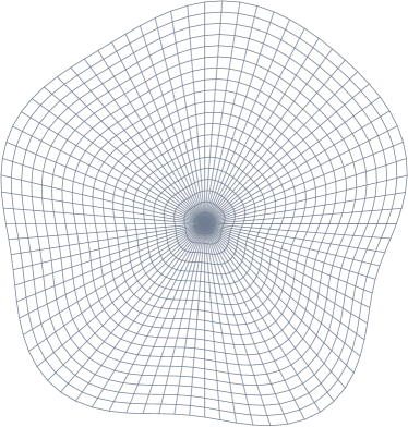
Figure 1. The domain under consideration, with a co-ordinate grid. Its boundary is used for the numerical tests.

We discretize the covariance operators by the (periodic) biorthogonal spline wavelets $\mathbf{\Psi}^{(d,\widetilde{d})}$ constructed in [14]. This class of wavelet bases has two parameters, namely the order $d$ of the underlying spline space and the number of vanishing moments $\widetilde{d}\geq d$, where $d+\widetilde{d}$ is even. When $\widetilde{d}$ increases, then the dual wavelet functions become more regular, enabling preconditioning of pseudodifferential operators of negative order.

For computing the compressed covariance matrix, the domain is scaled to unit diameter. Then, we choose $a=a^{\prime}=2$ and $d^{\prime}=d+(\widetilde{d}-d+r)/4$ in (3.19). This choice turned out to be robust for different applications. The $p\times p$ compressed covariance matrix can be assembled in cost which scales linearly with $p$ if exponentially convergent $hp$–quadrature methods are employed for the computation of matrix entries, cf. [13, 32, 34]. Further matrix operations such as matrix-vector multiplications admit additional a-posteriori compression which is here applied. This was found to reduce the number of nonzero entries by an additional factor between $2$ and $5$, see [18, Thm. 8.3]. The pattern of the compressed system matrix shows the typical “finger-band” structure, see also Figure 2.

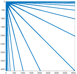
Figure 2. A-priori compression pattern for $p=4096$ wavelets in case of the Matérn covariance kernel $k_{1/2}$ and $\mathbf{\Psi}^{(2,6)}$ (left) and in case of the Matérn covariance kernel $k_{3/2}$ and $\mathbf{\Psi}^{(2,8)}$ (right). In the left and right matrix, only 5.0 % and 6.8 % of the matrix coefficients are relevant, respectively.

5.2. Condition numbers and compression rates

We choose first the correlation length $\ell=1$ and focus on the covariance operators for $k_{1/2}$ and $k_{3/2}$. From the inequality $d<\widetilde{d}+r$ for achieving optimal compression rates, we conclude that we need at least $\widetilde{d}=6$ vanishing moments to discretize $k_{1/2}$ and $\widetilde{d}=8$ vanishing moments to discretize $k_{3/2}$. In our experiments, we also include the borderline case of $\widetilde{d}=d-r$ vanishing moments, which leads only to a loglinear compression rate.

$k_{1/2}$
$p$	$J$	single-scale	nnz	$\mathbf{\Psi}^{(2,4)}$	nnz	$\mathbf{\Psi}^{(2,6)}$	nnz	$\mathbf{\Psi}^{(2,8)}$
32	5	$2.6\cdot 10^{3}$	100	$2.4\cdot 10^{2}$	100	$1.8\cdot 10^{2}$	100	$6.6\cdot 10^{2}$
64	6	$1.1\cdot 10^{4}$	80	$2.7\cdot 10^{2}$	88	$1.9\cdot 10^{2}$	98	$6.7\cdot 10^{2}$
128	7	$4.5\cdot 10^{4}$	60	$3.1\cdot 10^{2}$	65	$1.9\cdot 10^{2}$	71	$6.8\cdot 10^{2}$
256	8	$1.9\cdot 10^{5}$	40	$3.4\cdot 10^{2}$	42	$1.9\cdot 10^{2}$	48	$6.8\cdot 10^{2}$
512	9	$7.6\cdot 10^{5}$	25	$3.7\cdot 10^{2}$	26	$1.9\cdot 10^{2}$	30	$6.8\cdot 10^{2}$
1024	10	$3.1\cdot 10^{6}$	16	$3.9\cdot 10^{2}$	16	$1.9\cdot 10^{2}$	18	$6.8\cdot 10^{2}$
2048	11	$1.2\cdot 10^{7}$	9.4	$4.0\cdot 10^{2}$	9.0	$1.9\cdot 10^{2}$	10	$6.8\cdot 10^{2}$
4096	12	$5.0\cdot 10^{7}$	5.0	$4.2\cdot 10^{2}$	5.0	$1.9\cdot 10^{2}$	5.7	$6.8\cdot 10^{2}$

Table 1. Condition numbers and compression rates in case of the Matérn covariance kernel $k_{1/2}$. The compression rates validate the asymptotically linear behaviour. The condition numbers stay bounded for $\mathbf{\Psi}^{(2,6)}$ and $\mathbf{\Psi}^{(2,8)}$, whereas for $\mathbf{\Psi}^{(2,4)}$ a slight increase is observed.

$k_{3/2}$
$p$	$J$	single-scale	nnz	$\mathbf{\Psi}^{(2,6)}$	nnz	$\mathbf{\Psi}^{(2,8)}$	nnz	$\mathbf{\Psi}^{(2,10)}$
32	5	$3.2\cdot 10^{5}$	100	$2.3\cdot 10^{3}$	100	$1.9\cdot 10^{4}$	100	$1.9\cdot 10^{4}$
64	6	$5.8\cdot 10^{6}$	91	$3.3\cdot 10^{3}$	98	$2.3\cdot 10^{4}$	100	$2.0\cdot 10^{4}$
128	7	$1.1\cdot 10^{8}$	69	$4.9\cdot 10^{3}$	75	$2.5\cdot 10^{4}$	79	$2.0\cdot 10^{4}$
256	8	$1.9\cdot 10^{9}$	48	$6.9\cdot 10^{3}$	51	$2.6\cdot 10^{4}$	55	$2.0\cdot 10^{4}$
512	9	$3.3\cdot 10^{10}$	31	$1.0\cdot 10^{4}$	33	$2.6\cdot 10^{4}$	36	$2.0\cdot 10^{4}$
1024	10	$5.4\cdot 10^{11}$	19	$1.3\cdot 10^{4}$	20	$2.7\cdot 10^{4}$	21	$2.0\cdot 10^{4}$
2048	11	$8.8\cdot 10^{12}$	11	$1.8\cdot 10^{4}$	12	$2.7\cdot 10^{4}$	12	$2.1\cdot 10^{4}$
4096	12	$1.4\cdot 10^{14}$	6.7	$2.5\cdot 10^{4}$	6.8	$2.8\cdot 10^{4}$	7.0	$2.8\cdot 10^{4}$

Table 2. Condition numbers and compression rates in case of the Matérn covariance kernel $k_{3/2}$. The numerical compression rates validate the asymptotically linear behaviour. The numerical condition numbers stay bounded for $\mathbf{\Psi}^{(2,8)}$ and ${\mathbf{\Psi}}^{(2,10)}$, whereas for $\mathbf{\Psi}^{(2,6)}$ a slight increase is observed.

The numerical results are listed in Table 1 for the Matérn covariance kernel $k_{1/2}$ and in Table 2 for the Matérn covariance kernel $k_{3/2}$. We find therein the condition numbers and the a-priori compression rates for the discretization by $p=2^{J}$ piecewise linear hat functions and wavelets, respectively. It is seen from the column labeled “single-scale” that the condition number grows indeed by the factor $2^{|r|}$ in case of the discretization by piecewise linear hat functions. In contrast, the condition numbers in case of the discretization by wavelets is bounded for all choices of $\widetilde{d}$ except for the borderline case $\widetilde{d}=d-r$, where the condition numbers still grow, although quite moderately.

The compression rates, measured by the percentage of the number of nonzero coefficients (nnz) relative to $p^{2}$, are also good in the (borderline) case $\widetilde{d}=d-r$, although then only a loglinear compression rate can generally be expected. This is caused by wavelets with fewer vanishing moments tending to have smaller supports as is known to hold for the wavelets $\psi^{(d,\tilde{d})}$ from [14] which are presently used. Hence, we obtain less matrix coefficients in the system matrix which correspond to wavelets with overlapping supports. The compression pattern of the system matrices and $p=4096$ wavelets are displayed for the Matérn covariance kernel $k_{1/2}$ and $\mathbf{\Psi}^{(2,6)}$ on the left and in case of the Matérn covariance kernel $k_{3/2}$ and $\mathbf{\Psi}^{(2,8)}$ on the right panel of Figure 2.

5.3. Influence of the correlation length on the compression rates

We should finally comment on the dependence of the compression on the correlation length. Since we do not consider the correlation length in the a-priori compression, it has no effect on this compression. Nonetheless, the correlation length has a considerable effect on the a-posteriori compression. This can be seen in Figure 3, where we plotted the compression rates versus the correlation length in case of the Matérn covariance kernels $k_{1/2}$ and $k_{3/2}$ for a fixed level of resolution and wavelet basis (we use $\mathbf{\Psi}^{(2,6)}$ for $k_{1/2}$ and $\mathbf{\Psi}^{(2,8)}$ for $k_{3/2}$). While the a-priori compression rates are fixed, the a-posteriori compression improves as the correlation length decreases. This effect is clear as the correlation becomes more and more local, thus, the far-field interaction gets negligible.

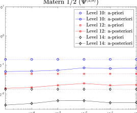
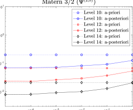
Figure 3. Influence of the correlation length on the compression rates (measured by the number of nonzero matrix entries in percent) in case of the Matérn covariance kernel $k_{1/2}$ and $\mathbf{\Psi}^{(2,6)}$ (left) and in case of the Matérn covariance kernel $k_{3/2}$ and $\mathbf{\Psi}^{(2,8)}$ (right). While the a-priori compression is unchanged, a-posteriori compression improves as the spatial correlation length decreases.

5.4. Decay of the diagonal entries

We next consider the behavior of the diagonal of the covariance matrices in wavelet coordinates. In Figure 4, we plotted the diagonal entries for the Matérn covariance kernels $k_{1/2}$, $k_{3/2}$, and $k_{5/2}$. We clearly see the transition between the levels at the abscissa values $2^{j}$. And indeed, if we compute the mean of the diagonal entries per level, the jump size between subsequent levels is precisely $4$, $16$, and $64$, which corresponds to $2^{-r}$ with $r$ being the operator order. As a consequence, the knowledge of the diagonal entries (or their mean) of just two subsequent levels is sufficient to estimate the coloring operator order, which, in turn, determines the path regularity and the tapering pattern.

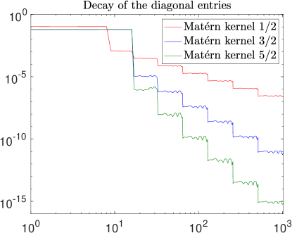
Figure 4. Size of the diagonal coefficients in case of the Matérn covariance kernels $k_{1/2}$, $k_{3/2}$, and $k_{5/2}$ for $\ell=1$ and $n=1$. We clearly observe the decay relative to the level, which depends on the order of the covariance operator. The jump between the level is of relative height $4$, $16$, and $64$ and reflects the operator order. Jump height is $2^{|r|}$, where $r=-(2\nu+1)$.

5.5. Fast simulation

We shall next illustrate the efficient numerical simulation of GRF samples on the algorithm from Subsection 4.1. We apply this algorithm to compute the square root of the compressed covariance matrix. To this end, we employ again the Matérn covariance kernel $k_{1/2}$ and $\mathbf{\Psi}^{(2,6)}$ as well as the Matérn covariance kernel $k_{3/2}$ and $\mathbf{\Psi}^{(2,8)}$. The correlation length is chosen as $\ell=1$. We numerically evaluate the $\|\cdot\|_{2}$ norm error between the exact matrix square root (computed by using the sqrtm-function from Matlab) and the approximation by (4.7) in dependence on the parameter $K$. A sensitive input parameter is $\widehat{\varkappa}_{\mathrm{R}}^{-1}$, which is the ratio between the smallest and largest eigenvalue. Therefore, we use its exact value on one hand and its over- or underestimation by a factor of two on the other hand, which accounts for numerical approximation. The results are displayed in Figure 5.

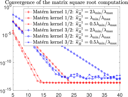
Figure 5. Convergence of the approximation (4.7) of the matrix square root of the diagonally scaled covariance matrix in case of the Matérn covariance kernel $k_{1/2}$ and $\mathbf{\Psi}^{(2,6)}$ and in case of the Matérn covariance kernel $k_{3/2}$ and $\mathbf{\Psi}^{(2,8)}$. The convergence rate is independent on the discretization level.

It tuns out that the convergence heavily depends on $\widehat{\varkappa}_{\mathrm{R}}^{-1}$ and, thus, on the condition number of the matrix under consideration. Especially, underestimation of $\widehat{\varkappa}_{\mathrm{R}}^{-1}$ seems to be harmless while overestimation slows down convergence considerably. Nonetheless, in any case, we achieve after for $K=40$ machine precision. Although the computations have been only carried out for fixed discretization level (namely, for $p=1024$ wavelets), we obtain exactly the same plots for other values of $p$ as the condition number of the covariance matrix stays constant in accordance with Tables 1 and 2.

5.6. Covariance estimation

We shall next illustrate the multilevel Monte Carlo estimation of the covariance matrix. To that end, we consider the $\ell^{2}$-difference between the original (uncompressed) covariance matrix and its approximation by the multilevel Monte Carlo method, using wavelet matrix compression. As test case, we consider the Matèrn kernel $k_{1/2}$, which is of order $-2$. Consequently, it holds $r=1$, $n=1$, and $t=t^{\prime}=0$ in Section 4.2. The wavelet basis used to discretize the covariance matrix is $\mathbf{\Psi}^{(2,6)}$. For the Monte Carlo sampling, we choose the fixed number of $\widetilde{M}_{J}=100$ samples on the finest level $J$ of spatial resolution and increase the number $\tilde{M}_{j}$ of MC samples by the factor $2^{2(n+\alpha)/3}=2$ when passing from spatial resolution level $j$ to $j-1$, $1\leq j\leq J$.

There, we chose the borderline case $\alpha=1/2$. This essentially yields the convergence order $2^{J/2}$ of the multilevel Monte Carlo method.

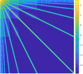
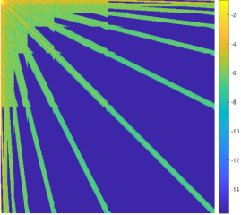
Figure 6. Truth covariance matrix (left) in wavelet representation and its multilevel Monte Carlo estimation (right) for $p=512$ parameters. Spatial dimension $d=1$, Matèrn-covariance kernel $k_{1/2}$, spatial correlation length $\ell=1$, wavelet $\mathbf{\Psi}^{(2,6)}$.

$p$	$J$	$\widetilde{M_{j}}$	$\ell^{2}$-error
8	3	51200	$1.1\cdot 10^{-1}$	—
16	4	25600	$5.4\cdot 10^{-2}$	(2.1)
32	5	12800	$4.9\cdot 10^{-2}$	(1.1)
64	6	6400	$2.9\cdot 10^{-2}$	(1.7)
128	7	3200	$1.9\cdot 10^{-2}$	(1.5)
256	8	1600	$1.3\cdot 10^{-2}$	(1.4)
512	9	800	$1.1\cdot 10^{-2}$	(1.3)
1024	10	400	$8.5\cdot 10^{-3}$	(1.2)
2048	11	200	$5.3\cdot 10^{-3}$	(1.6)
4096	12	100	$2.9\cdot 10^{-3}$	(1.3)

Table 3. MLMC Covariance estimation. Sample sizes $\widetilde{M}_{j}$ and accuracy of the multilevel Monte Carlo covariance estimation, with $\widetilde{M}_{J}=100$, and with $\widetilde{M}_{j}=\widetilde{M}_{J}2^{J-j}$; presented here for $J=12$. Estimation error in operator norm with respect to the (densely populated), exact covariance matrix ${\mathbf{C}}_{p}$ in wavelet coordinates.

The results are presented in Table 3. Here, one figures out the sample numbers $\widetilde{M_{j}}$ per level $j$ in case of discretization level $J=12$. For smaller levels, one just has to remove the largest numbers accordingly. We moreover tabulated the $\ell^{2}$-error between the (uncompressed) covariance matrix and its estimate, where the given numbers correspond to the mean of 10 runs. The convergence order is like expected, as validated by the contraction factor $1.41$ between the levels, which is approximately observed. In Figure 6, one finds the original covariance matrix of size $512\times 512$ on the left and its Monte Carlo estimate on the right. In the (single-level) MC estimate, no a-priori (oracle) information on the sparsity pattern has been provided. Still, the compression pattern has clearly been identified.

5.7. Sparse approximate kriging

We next consider the kriging approach presented in Subsection 4.3 and especially in Remark 4.7. To this end, we consider that we have given $K=32$ locally supported functionals $g_{i}$ which are equidistantly distributed at the boundary $\Gamma$ of the computational domain under consideration. Then, using $p=512$ piecewise linear ansatz functions and wavelets $\mathbf{\Psi}^{(2,6)}$, we obtain the matrix representation (4.20) which is illustrated in Figure 7.

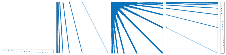
Figure 7. Sparse factorization of the approximate kriging matrix ${\bf G{\mathbf{C}}^{\varepsilon}_{p}G}^{\top}={\bf G}_{\tilde{\phi}}{\bf T}_{\tilde{\phi}\to\tilde{\psi}}^{\top}{\mathbf{C}}_{p}^{\varepsilon}{\bf T}_{\tilde{\phi}\to\tilde{\psi}}\mathbf{G}_{\tilde{\phi}}^{\top}$ according to Theorem 4.6, Remark 4.7 and (4.20).

We emphasize that the matrix which arises from the fast wavelet transform (second and fourth matrix in Figure 7) has obviously $\mathcal{O}(p\log p)$ nonzero matrix coefficients. However, its application to a vector can be realized numerically in $\mathcal{O}(p)$ operations with a very small constant that depends on the filter length of the wavelets.

5.8. Computations of a GRF on $\mathbb{S}^{2}$

After having illustrated the theoretical findings on a manifold in two spatial dimensions, we shall also demonstrate the wavelet compression for GRFs in spatial dimension $n=2$. We consider the simulation of the centered GRF $\mathcal{Z}$ on the unit sphere $\mathcal{M}=\mathbb{S}^{2}\subset\mathbb{R}^{3}$. The covariance kernel under consideration is assumed to be the Matèrn kernel $k_{1/2}$, defined in terms of the geodesic distance on $\mathbb{S}^{2}$, with unit geodesic correlation length. We apply piecewise constant wavelets with three vanishing moments, as constructed in [33]. Since (3.19) is violated and the wavelets are also not suitable for preconditioning since $\widetilde{\gamma}=1/2$, we perform the matrix compression as for an operator of order 0. This is justified since also the Karhunen-Loéve expansion is computed with respect to $L^{2}(\mathbb{S}^{2})$. As pointed out in [31], the Cholesky decomposition of the compressed covariance matrix can efficiently computed with nested dissection reordering, compare Figure 8. Here, we see the original matrix pattern of the compressed covariance operator on the left, its reordered version in the middle, and the resulting Cholesky factor on the right. Indeed, the number of nonzero matrix coefficients of the Cholesky factor is only about 4–5 times higher than that of the compressed covariance operator (compare Table 4). This appears to be consistent with [53, Proposition 1].

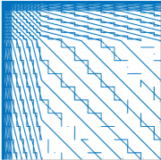
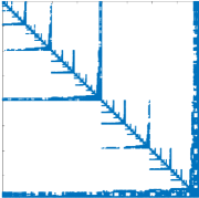
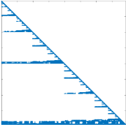
Figure 8. GRF on $\mathcal{M}=\mathbb{S}^{2}$: sparsity pattern of the compressed covariance operator in wavelet coordinates (left), its nested dissection, “skyline” reordering (middle), and sparsity pattern of the exact Cholesky factor (right) of the compressed, reordered covariance matrix ${\mathbf{C}}_{p}\in\mathbb{R}^{p\times p}$ for $p=393216$. Consistent with [53, Proposition 1], see also [25, Chap. 4.2].

The efficient drawing of numerically approximated random samples proceeds as follows. Let ${\bf C}_{J}^{\psi}$ denote the compressed covariance operator, ${\bf C}_{J}^{\psi}={\bf L}_{J}^{\psi}\big{(}{\bf L}_{J}^{\psi}\big{)}^{\top}$ its Cholesky decomposition, and ${\bf G}_{J}^{\phi}$ the mass matrix with respect to the piecewise constant single-scale basis, which is a diagonal matrix. Then, for a uniformly normally distributed random vector ${\bf X}(\omega)$, the random vector ${\bf Y}(\omega)=\big{(}{\bf G}_{J}^{\phi}\big{)}^{-1}{\bf T}_{\psi\to\phi}{\bf L}_{J}^{\psi}{\bf X}(\omega)$ represents the sought Gaussian random field on the unit sphere $\mathbb{S}^{2}$, expressed with respect to the piecewise constant single-scale basis. As can be seen in the last column of Table 4, the computation time per sample is very small. Four realizations can be found in Figure 9.

Sphere
$p$	$J$	nnz(${\bf C}_{J}$)	cpu(${\bf C}_{J}$)	nnz(${\bf L}_{J}$)	cpu(${\bf L}_{J}$)	cpu(sample)
6144	5	4.70	18	10.3	0.65	0.0017
24576	6	1.22	113	4.43	5.1	0.015
98304	7	0.43	692	1.68	26	0.096
393216	8	0.12	4108	0.59	151	0.46
1572864	9	0.03	23374	0.20	865	2.7

Table 4. Compression rates and computing times in case of the Matérn covariance kernel $k_{1/2}$ on the sphere. Once the Cholesky decomposition has been computed, each sample can be computed extremely fast.

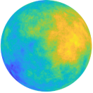
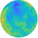
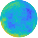
Figure 9. Four realizations of a Gaussian random field on $\mathbb{S}^{2}$ for the Matèrn covariance $k_{1/2}$ with respect to the geodesic distance.

All the computations have been carried out on a compute server with dual 20-core Intel Xeon E5-2698 v4 CPU at 2.2 GHz and 768 GB RAM. The computation of the compressed covariance operator has been done with the help of a C-program on a single core in line with [34], while nested dissection and the Cholesky factorization have been computed by using Matlab.

Let us emphasize that, according to [47, 60], wavelets with the same properties are available also in case of unstructured triangulations. Furthermore, the efficient assembly of the system matrix in case of such wavelets has been presented in [2]. Therefore, the algorithm proposed here can be expected to perform efficiently also in practical situations, e.g., for high-dimensional graphical models, where the present hypotheses may not hold or may be difficult to verify.

6. Conclusions

For a GRF $\mathcal{Z}$ indexed by a smooth manifold $\mathcal{M}$ which is obtained by “coloring” white noise $\mathcal{W}$ with an elliptic, self-adjoint pseudodifferential operator $\mathcal{A}$ as in (2.1), we proved that in suitable wavelet coordinates in $L^{2}(\mathcal{M})$ precision and covariance operators $\mathcal{P}$ and $\mathcal{C}$ of $\mathcal{Z}$ both admit numerical approximations that are optimally sparse. This is to say, for any number $p\in\mathbb{N}$ of leading wavelet coordinates of $\mathcal{Z}$, the $p\times p$ sections ${\mathbf{P}}_{p}$ and ${\mathbf{C}}_{p}$ of equivalent, bi-infinite matrix representations ${\mathbf{P}},{\mathbf{C}}\in\mathbb{R}^{\mathbb{N}\times\mathbb{N}}$ of $\mathcal{C}$ and $\mathcal{P}$ admit sparse approximations ${{\mathbf{P}}}_{p}^{\varepsilon}$ and ${{\mathbf{C}}}_{p}^{\varepsilon}$ with $\mathcal{O}(p)$ nonzero entries that are optimally consistent with $\mathcal{C}$ and $\mathcal{P}$. The location of the $\mathcal{O}(p)$ “essential” entries of ${{\mathbf{P}}}_{p}^{\varepsilon}$ and ${{\mathbf{C}}}_{p}^{\varepsilon}$ is universal (for the pseudodifferential colorings under consideration) and can either be given a-priori, based on regularity of $\mathcal{Z}$, or numerically estimated a-posteriori from the decay of the wavelet coefficients, see Figure 4. This a-posteriori compression is facilitated by a wavelet representation of the GRF $\mathcal{Z}$, since sample-wise smoothness of $\mathcal{Z}$ in Sobolev and Besov scales on $\mathcal{M}$ is encoded in the decay (of the components) of the random coefficient sequence $\widetilde{\mathbf{z}}$ corresponding to the MRA. We furthermore have proven that diagonal preconditioning renders the condition numbers of both, ${{\mathbf{P}}}_{p}^{\varepsilon}$ and ${{\mathbf{C}}}_{p}^{\varepsilon}$, bounded uniformly with respect to the number of parameters, $p$.

The theory and the algorithms do not rely on stationarity of the GRFs. Furthermore, the assumption of self-adjointness on the coloring operator $\mathcal{A}$ was made only for ease of presentation. In the general case $\mathcal{A}^{*}\neq\mathcal{A}$ the covariance operator $\mathcal{C}=(\mathcal{A}^{*}\mathcal{A})^{-1}$ will still be self-adjoint and the GRF $\mathcal{Z}=\mathcal{A}^{-1}\mathcal{W}$ colored by $\mathcal{A}$ has the same distribution as a GRF colored by the self-adjoint operator $|\mathcal{A}|=(\mathcal{A}^{*}\mathcal{A})^{1/2}$.

The wavelet-based numerical covariance compression and preconditioning is in line with work to exploit a-priori structural hypotheses on covariance matrix sparsity for the efficient numerical approximation of (samples of) GRFs and of algorithms to estimate their covariance operators and functions. As one possible extension of the present analysis, the a-priori known locations of the $\mathcal{O}(p)$ many nonzero entries of ${{\mathbf{P}}}_{p}^{\varepsilon}$ and ${{\mathbf{C}}}_{p}^{\varepsilon}$ may be leveraged in oracle versions of covariance estimation methodologies such as (group) LASSO. These are well established for statistical inference in high-dimensional, graphical models (e.g. [42, Condition A1]), where numerical constructions of MRAs have been proposed e.g. in [15].

The hierarchic nature of wavelet MRAs naturally facilitates novel, multilevel versions of established covariance estimation algorithms as described in [7, 6, 52, 42] and the references there. They amount to sampling the GRF $\mathcal{Z}$ represented in the MRA with a number of samples which depends on the spatial resolution level, with large numbers of low-resolution samples, and only few samples at the highest spatial resolution. We presented one such multilevel estimation algorithm and proved its asymptotically optimal, linear complexity for all pseudodifferential colorings under consideration. We introduced a novel, numerically sparse multilevel algorithm for kriging, i.e., for the spatial prediction given data. This is only a first application of the present results to methodologies in spatial statistics and more are conceivable. For instance, the computational benefits of wavelet representations may be exploited for computationally challenging tasks such as statistical inference of parameters.

Appendix A Pseudodifferential operators on manifolds

We consider orientable manifolds satisfying Assumption 2.1(I). In the case that $\mathcal{M}$ is not orientable, there exists a covering manifold $\widetilde{\mathcal{M}}$ of $\mathcal{M}$ with two sheets such that $\widetilde{\mathcal{M}}$ is orientable [3, Thm. I.58] and of dimension $n\geq 1$.

A.1. Surface differential calculus

A tangent vector at $x\in\mathcal{M}$ is a mapping $X\colon f\to X(f)\in\mathbb{R}$ which is defined on the set of functions $f$ that are differentiable in a neighborhood of $x$ which satisfies a) for $\lambda,\mu\in\mathbb{R}$, $X(\lambda f+\mu g)=\lambda X(f)+\mu X(g)$, b) $X(f)=0$if $f$ is flat, c) $X(fg)=f(x)X(g)+g(x)X(f)$. The tangent space $T_{x}(\mathcal{M})$ to $\mathcal{M}$ at $x\in\mathcal{M}$ is the set of tangent vectors at $x$. In any coordinate system $\{x^{i}\}$ in $\mathcal{M}$ at $x$, the vectors $\partial/\partial x^{i}$ defined by $(\partial/\partial x^{i})_{x}(f)=[\partial(f\circ\varphi^{-1})/\partial x^{i}]_{\varphi(x)}$ belong to $T_{x}(\mathcal{M})$, and form a basis of the tangent vector space at $x\in\mathcal{M}$. Here, $\varphi$ is any diffeomorphism on a neighborhood of $x$. Its dual vector space is denoted by $T_{x}^{*}(\mathcal{M})$. The tangent space $T(\mathcal{M})$ to $\mathcal{M}$ is $\bigcup_{x\in\mathcal{M}}T_{x}(\mathcal{M})$, the dual tangent space $T^{*}(\mathcal{M})$ is $\bigcup_{x\in\mathcal{M}}T^{*}_{x}(\mathcal{M})$. The tangent space $T(\mathcal{M})$ carries a vector fiber bundle structure. More generally, for $r,s\in\mathbb{N}$, the fiber bundle $T^{r}_{s}(\mathcal{M})$ of $(r,s)$ tensors is $\bigcup_{x\in\mathcal{M}}T_{x}(\mathcal{M})^{\otimes^{r}}\otimes T_{x}^{*}(\mathcal{M})^{\otimes^{s}}$.

The manifold $\mathcal{M}$ gives rise to the compact metric space $(\mathcal{M},\operatorname{dist}(\,\cdot\,,\,\cdot\,))$, where the distance $\operatorname{dist}(\,\cdot\,,\,\cdot\,)$ can be chosen, for example, as the geodesic distance in $\mathcal{M}$ of two points $x,x^{\prime}\in\mathcal{M}$, see [3, Prop. I.35].

A.1.1. Coordinate charts and triangulations

Provided that the manifold $\mathcal{M}$ of dimension $n$ satisfies Assumption 2.1(I), it can be locally represented as parametric surface consisting of smooth coordinate patches. Specifically, denote by $\Box=[0,1]^{n}$ the unit cube. Then we assume that $\mathcal{M}$ is partitioned into a finite number $M$ of closed patches $\mathcal{M}_{i}$ such that

$$\mathcal{M}=\bigcup_{i=1}^{M}\mathcal{M}_{i},\quad\mathcal{M}_{i}=\gamma_{i}(\Box),\;\;i=1,\ldots,M\;.$$

Here, each $\gamma_{i}\colon\Box\to\mathcal{M}_{i}$ is assumed to be a smooth diffeomorphism. We also assume that there exist smooth extensions $\widetilde{\mathcal{M}}_{i}\supset\mathcal{M}_{i}$ and $\widetilde{\gamma}_{i}\colon\widetilde{\Box}\to\widetilde{\mathcal{M}}_{i}$ such that $\widetilde{\gamma}_{i}|_{\Box}=\gamma_{i}$, where $\widetilde{\Box}=(-1,2)^{n}$. Note that, in the notation of Section 2, $G=\widetilde{\Box}$.

The intersections $\mathcal{M}_{i}\cap\mathcal{M}_{j}$ for $i\neq j$ are either assumed to be empty or to be diffeomorphic to $[0,1]^{k}$ for some $0\leq k<n$. We assume the charts $\gamma_{i}$ to be $C^{0}$-compatible in the sense that for every $\hat{x}\in\mathcal{M}_{i}\cap\mathcal{M}_{i^{\prime}}$ exists a bijective mapping $\Theta\colon\Box\to\Box$ such that $(\gamma_{i^{\prime}}\circ\Theta)(x)=\hat{x}$ for $x=(x_{1},\ldots,x_{n})\in\Box$ with $\gamma_{i}(x)=\hat{x}$. Note that $C^{0}$-compatibility admits $\mathcal{M}=\partial G$ for certain polytopal domains $G$. In the case that $\mathcal{M}=\partial G$ is smooth, we shall assume that the extensions satisfy $\widetilde{\mathcal{M}}_{i}\subset\mathcal{M}$ and that the charts $\gamma_{i}$ are smoothly compatible.

In the construction of MRAs on $\mathcal{M}$, we shall require triangulations of $\mathcal{M}$. We shall introduce these in the Euclidean parameter domain $\Box$ and lift them to the coordinate patches $\mathcal{M}_{i}$ on $\mathcal{M}$ via the charts $\gamma_{i}$.

A mesh of refinement level $j$ on $\mathcal{M}$ is obtained by dyadic subdivisions of depth $j$ of $\Box$ into $2^{jn}$ subcubes $C_{j,k}\subseteq\Box$, where the multi-index $k=(k_{1},\ldots,k_{n})\in\mathbb{N}_{0}^{n}$ tags the location of $C_{j,k}$ with $0\leq k_{m}<2^{j}$. With this construction in each co-ordinate patch, and taking into account the inter-patch compatibility of the charts $\gamma_{i}$, this results in a regular quadrilateral triangulation of $\mathcal{M}$ consisting of $2^{jn}M$ cells $\Gamma_{i,j,k}:=\gamma_{i}(C_{j,k})\subset\mathcal{M}_{i}\subset\mathcal{M}$.

A.1.2. Sobolev spaces

Let $\mathcal{M}$ denote a compact manifold as in Section A.1.1. Sobolev spaces on $\mathcal{M}$ are invariantly defined in the usual fashion, i.e., in local coordinates of a smooth atlas $\{\widetilde{\gamma}_{i}\}_{i=1}^{M}$ of coordinate charts on $\mathcal{M}$.

As in Assumption 2.1(I), we assume that $\mathcal{M}$ has dimension $n\in\mathbb{N}$, $\partial\mathcal{M}=\emptyset$, and is equipped with a (surface) measure $\mu$. It is given in terms of the first fundamental form on $\mathcal{M}$ which, on $\mathcal{M}_{i}$, is given by

(A.1) $$K_{i}(x)=\bigl{(}\partial_{j}\widetilde{\gamma}_{i}(x)\cdot\partial_{j^{\prime}}\widetilde{\gamma}_{i}(x)\bigr{)}_{j,j^{\prime}=1}^{n},\quad x\in\widetilde{\gamma}_{i}^{-1}(\mathcal{M}_{i}).$$

The matrix $K_{i}$ in (A.1) is symmetric and positive definite uniformly in $x\in\widetilde{\mathcal{M}}_{i}$. The $L^{2}(\mathcal{M})$ inner product on $\mathcal{M}$ can then be expressed in the local chart coordinates via

$$(v,w)_{L^{2}(\mathcal{M})} :=\int_{\mathcal{M}}v(x)w(x)\,\mathrm{d}\mu(x)$$

$$=\sum_{i=1}^{M}\int_{\widetilde{\Box}}((\chi_{i}v)\circ\widetilde{\gamma}_{i})(x)((\chi_{i}w)\circ\widetilde{\gamma}_{i})(x)\sqrt{\det(K_{i}(x))}\,\mathrm{d}x,$$

where $\{\chi_{i}\}_{i=1}^{M}$ denotes a smooth partition of unity which is subordinate to the atlas $\{\widetilde{\gamma}_{i}\}_{i=1}^{M}$. For $1\leq p\leq\infty$, $L^{p}(\mathcal{M})$ shall denote the usual space of real-valued, strongly measurable maps $v\colon\mathcal{M}\to\mathbb{R}$ which are $p$-integrable with respect to $\mu$.

Sobolev spaces on $\mathcal{M}$ are invariantly defined by lifting their Euclidean versions on $\widetilde{\Box}$ to $\widetilde{\mathcal{M}}_{i}$ via $\widetilde{\gamma}_{i}$. For $s\geq 0$, the respective norm on $H^{s}(\mathcal{M})$ may be defined by

$$\|v\|_{H^{s}(\mathcal{M})}:=\sum_{i=1}^{M}\|(\chi_{i}v)\circ\widetilde{\gamma}_{i}\|_{H^{s}(\widetilde{\Box})}.$$

This definition is equivalent to the definition of $H^{s}(\mathcal{M})$ and $\|\,\cdot\,\|_{H^{s}(\mathcal{M})}$ in (2.5). For further details the reader is referred to [37, pp. 30–31 of Appendix B] and the references therein. (Note that the proof of this equivalence on the sphere $\mathcal{M}=\mathbb{S}^{2}$ as elaborated in [37] exploits only compactness and smoothness of $\mathbb{S}^{2}$. Thus, it can be generalized to any manifold as considered in this work.)

For $s<0$, the spaces $H^{s}(\mathcal{M})$ are defined by duality, here and throughout identifying $L^{2}(\mathcal{M})$ with its dual space.

A.2. (Pseudo)differential operators

We review basic definitions and notation from the Hörmander–Kohn–Nirenberg calculus of pseudodifferential operators, to the extent that they are needed in our analysis of covariance kernels and operators.

A.2.1. Basic definitions

Let $G$ be an open, bounded subset of $\mathbb{R}^{n}$, $r$, $\rho$, $\delta\in\mathbb{R}$ with $0\leq\rho\leq\delta\leq 1$. The Hörmander symbol class $S^{r}_{\rho,\delta}(G)$ consists of all $b\in C^{\infty}(G\times\mathbb{R}^{n})$ such that, for all $K\subset\subset G$ and for any $\alpha,\beta\in\mathbb{N}_{0}^{n}$, there is a constant $C_{K,\alpha,\beta}>0$ with

(A.2) $$\forall x\in K,\;\;\forall\xi\in\mathbb{R}^{n}:\quad\bigl{|}\partial^{\beta}_{x}\partial^{\alpha}_{\xi}b(x,\xi)\bigr{|}\leq C_{K,\alpha,\beta}(1+|\xi|)^{r-\rho|\alpha|+\delta|\beta|}.$$

When the set $G$ is clear from the context, we write $S^{r}_{\rho,\delta}$. In what follows, we shall restrict ourselves to the particular case $\rho=1$, $\delta=0$, and consider $S^{r}_{1,0}$. In addition, we write $S^{-\infty}_{1,0}:=\bigcap_{r\in\mathbb{R}}S^{r}_{1,0}$. A symbol $b\in S^{r}_{1,0}$ gives rise to a pseudodifferential operator $B$ via the relation (2.3).

When $b\in S^{r}_{1,0}$, the operator $B$ is said to belong to $OPS^{r}_{1,0}(G)$ and it is (in a suitable topology) a continuous operator $B\colon C_{0}^{\infty}(G)\to C^{\infty}(G)$, cf. [61, Thm. II.1.5]. We write $OPS^{-\infty}(G)=\bigcap_{r\in\mathbb{R}}OPS^{r}_{1,0}(G)$. We say that the operator $B\in OPS^{r}_{1,0}(G)$ is elliptic of order $r\in\mathbb{R}$ if, for each compact $K\subset\subset G$, there exist constants $C_{K}>0$ and $R>0$ such that

$$\forall x\in K,\;\;\forall|\xi|\geq R:\quad|b(x,\xi)|\geq C_{K}\bigl{(}1+|\xi|^{2}\bigr{)}^{r}.$$

A.2.2. (Pseudo)differential operators on manifolds

We suppose Assumption 2.1. Having introduced the class $OPS^{r}_{1,0}(G)$ for an Euclidean domain $G$, the operator class $OPS^{r}_{1,0}(\mathcal{M})$ is defined by the usual “lifting to $\mathcal{M}$ in local coordinates” as described, e.g., in [61, Sec. II.5]. The definition is based on the behavior of $OPS^{r}_{1,0}(G)$ under smooth diffeomorphic changes of coordinates which we consider first.

Let $G,\mathcal{O}\subset\mathbb{R}^{n}$ be open and let $\gamma\colon G\to\mathcal{O}$ be a diffeomorphism. Consider $B\in OPS^{r}_{1,0}(G)$, so that $B\colon C_{0}^{\infty}(G)\to C^{\infty}(G)$. We define the transported operator $\widetilde{B}$ by

$$\widetilde{B}\colon C^{\infty}_{0}(\mathcal{O})\to C^{\infty}(\mathcal{O}),\quad u\mapsto B(u\circ\gamma)\circ\gamma^{-1}.$$

For $r\in\mathbb{R}$, we then consider $OPS^{r}_{1,0}(\mathcal{M})$, the Hörmander class of pseudodifferential operators on $\mathcal{M}$ (investigated earlier by Kohn and Nirenberg [44]). We alert the reader to the use of the notation $OPS^{r}(\mathcal{M})$ for the so-called classical pseudo- differential operators which afford (pseudohomogeneous) symbol expansions and comprise a strict subset of $OPS^{r}_{1,0}(\mathcal{M})$, see, e.g., [58].

Pseudodifferential operators in $OPS^{r}_{1,0}(\mathcal{M})$ on manifolds $\mathcal{M}$ are defined in local coordinates. A linear operator $\mathcal{B}\colon C^{\infty}(\mathcal{M})\to C^{\infty}(\mathcal{M})$ is a pseudodifferential operator of order $r\in\mathbb{R}$ on $\mathcal{M}$, $\mathcal{B}\in OPS^{r}_{1,0}(\mathcal{M})$, if for any finite, smooth partition of unity $\bigl{\{}\chi_{i}\in C_{0}^{\infty}(\widetilde{\mathcal{M}}_{i}):i=1,\ldots,\bar{m}\bigr{\}}$ with respect to any atlas $\bigl{\{}\bigl{(}\widetilde{\mathcal{M}}_{i},\widetilde{\gamma}_{i}\bigr{)}\bigr{\}}_{i=1}^{\bar{m}}$ of $\mathcal{M}$ all transported operators satisfy

(A.3) $$f\mapsto B_{i,i^{\prime}}f=f\mapsto\bigl{[}\bigl{(}\mathcal{B}[\chi_{i}(f\circ\widetilde{\gamma}_{i}^{-1})]\bigr{)}\chi_{i^{\prime}}\bigr{]}\circ\widetilde{\gamma}_{i^{\prime}}\in OPS^{r}_{1,0}(\widetilde{\gamma}_{i}^{-1}(\widetilde{\mathcal{M}}_{i}))\quad\forall i,i^{\prime}=1,\ldots,\bar{m}.$$

The class of all such operators is denoted $OPS^{r}_{1,0}(\mathcal{M})$. Importantly, $OPS^{r}_{1,0}(\mathcal{M})$ defined in this way does not depend on the choice of the atlas of $\mathcal{M}$ and is invariantly defined [61, Sec. II.5], [41, Def. 18.1.20].

A.2.3. Principal symbols

For a bounded, open set $\mathcal{O}\subset\mathbb{R}^{n}$, the principal symbol $b_{0}(x,\xi)$ of $B\in OPS^{r}_{1,0}(\mathcal{O})$ is the equivalence class in $S^{r}_{1,0}(\mathcal{O})/S^{r-1}_{1,0}(\mathcal{O})$ (see, e.g., [61, p. 49]). Any member of the equivalence class will be called a principal symbol of $B$. For $\mathcal{B}\in OPS^{r}_{1,0}(\mathcal{M})$, its principal symbol $b_{0}(x,\xi)$ is invariantly (with respect to the choice of atlas on $\mathcal{M}$) defined on $T^{*}(\mathcal{M})$ (see [61, Eq. (5.6)]).

A.2.4. Pseudodifferential calculus

The symbol class $S^{r}_{1,0}$ admits a symbolic calculus (e.g., [61, Prop. II.1.3]). In the sequel, we assume all pseudodifferential operators to be properly supported, see [61, Def. II.3.6]. This is not restrictive, as every $\mathcal{B}\in OPS^{r}_{1,0}(\mathcal{M})$ can be written as $\mathcal{B}=\mathcal{B}_{1}+\mathcal{R}$, where $\mathcal{B}_{1}\in OPS^{r}_{1,0}(\mathcal{M})$ is properly supported and where $\mathcal{R}\in OPS^{-\infty}(\mathcal{M})$ [41, Prop. 18.1.22].

Proposition A.1.

Let $r,t\in\mathbb{R}$ and $\mathcal{A}\in OPS^{r}_{1,0}(\mathcal{M})$, $\mathcal{B}\in OPS^{t}_{1,0}(\mathcal{M})$ be properly supported. Then, it holds

1. $\mathcal{A}+\mathcal{B}\in OPS^{\max\{r,t\}}_{1,0}(\mathcal{M})$,

2. $\mathcal{A}\mathcal{B}\in OPS^{r+t}_{1,0}(\mathcal{M})$,

3. $\forall s\in\mathbb{R}:\;\mathcal{A}\colon H^{s}(\mathcal{M})\to H^{s-r}(\mathcal{M})$ is continuous.

Proof.

The symbol class $S^{r}_{1,0}$ is constructed such that by (A.2), $S^{r}_{1,0}\subseteq S^{\max\{r,t\}}_{1,0}$ and also $S^{t}_{1,0}\subseteq S^{\max\{r,t\}}_{1,0}$. Assertion (i) follows from the construction of the class $OPS^{r}_{1,0}(\mathcal{M})$ via an atlas, see Section A.2.2.

Recall the atlas $\{\widetilde{\gamma}_{i}\}_{i=1}^{M}$ of $\mathcal{M}$ with subordinate smooth partition of unity $\{\chi_{i}\}_{i=1}^{M}$. The transported operators $A_{i,i^{\prime}}$ and $B_{i,i^{\prime}}$ defined according to (A.3) belong to $OPS^{r}_{1,0}(\widetilde{\Box})$ and to $OPS^{t}_{1,0}(\widetilde{\Box})$. By [61, Thm. II.4.4], $A_{j,j^{\prime}}B_{j,j^{\prime}}\in OPS^{r+t}_{1,0}(\widetilde{\Box})$. Thus, claim (ii) holds by the construction of the class $OPS^{r+t}_{1,0}(\mathcal{M})$ in Subsection A.2.2.

Finally, the third assertion (iii) follows from [61, Thm. II.6.5], which is elucidated on [61, p. 53 of Sec. II.7]. ∎

Proposition A.2.

Let $r\in\mathbb{R}$ and $\mathcal{A}\in OPS^{r}_{1,0}(\mathcal{M})$ be self-adjoint, positive definite, and elliptic, i.e., there exists a constant $a_{-}>0$ such that

$$\forall w\in H^{r/2}(\mathcal{M}):\quad\langle\mathcal{A}w,w\rangle\geq a_{-}\|w\|_{H^{r/2}(\mathcal{M})}^{2}.$$

Then, for every $\beta\in\mathbb{R}$, $\mathcal{A}^{\beta}\in OPS^{\beta r}_{1,0}(\mathcal{M})$.

Proof.

Since $a_{-}>0$, $\mathcal{A}$ is invertible. The assertion follows from [58, Thm. 3]. ∎

Appendix B Multiresolution bases on manifolds

In this section we briefly explain how the single-scale basis $\mathbf{\Phi}_{j}$, the dual single-scale basis $\widetilde{\mathbf{\Phi}}_{j}$ as well as the biorthogonal complement bases $\mathbf{\Psi}_{j}$ and $\widetilde{\mathbf{\Psi}}_{j}$ in (3.3), (3.4) and (3.6) can be constructed on a manifold $\mathcal{M}$ which satisfies Assumption 2.1(I). Furthermore, we collect some of their basic properties.

We recall from (3.3) that, for $j>j_{0}$, the subspaces $V_{j}\subset V_{j+1}\subset\ldots\subset L^{2}(\mathcal{M})$ are spanned by single-scale bases $\mathbf{\Phi}_{j}:=\{\phi_{j,k}:k\in\Delta_{j}\}$, where $\Delta_{j}$ denote suitable index sets describing spatial localization of the $\phi_{j,k}$. Furthermore, the subspaces are of cardinality $\dim(V_{j})=\mathcal{O}(2^{nj})$. We assume elements $\phi_{j,k}\in V_{j}$ to be normalized in $L^{2}(\mathcal{M})$, and their supports to scale according to $\operatorname{diam}(\operatorname{supp}\phi_{j,k})\simeq 2^{-j}$. We associate with these bases so-called dual single-scale bases $\widetilde{\mathbf{\Phi}}_{j}:=\{\widetilde{\phi}_{j,k}:k\in\Delta_{j}\}$, for which one has $\langle\phi_{j,k},\widetilde{\phi}_{j,k^{\prime}}\rangle=\delta_{k,k^{\prime}}$ for $k,k^{\prime}\in\Delta_{j}$. Such dual systems of one-scale bases on $\mathcal{M}$ can be lifted in charts $\mathcal{M}_{j}$ via parametrizations $\gamma_{j}$ from tensor products of univariate systems in the parameter domains $\Box\subset\mathbb{R}^{n}$. For example, for primal bases $\mathbf{\Phi}_{j}$ obtained from tensorized, univariate B-splines of order $d$ in $\Box$ with dual bases of order $\widetilde{d}$ such that $d+\widetilde{d}$ is even, the $\mathbf{\Phi}_{j}$ and $\widetilde{\mathbf{\Phi}}_{j}$ have approximation orders $d$ and $\widetilde{d}$, respectively, see (3.2). The respective regularity indices $\gamma$ and $\widetilde{\gamma}$, see (3.2), satisfy $\gamma=d-1/2$, whereas $\widetilde{\gamma}\sim\widetilde{d}$. We refer to [47, 20, 48] for detailed constructions.

The biorthogonality of the systems $\mathbf{\Phi}_{j}$, $\widetilde{\mathbf{\Phi}}_{j}$ allows to introduce canonical projectors $Q_{j}$ and $Q^{*}_{j}$ for $j\in\mathbb{N}$ with $j>j_{0}$:

$$Q_{j}v:=\sum_{k\in\Delta_{j}}\langle v,\widetilde{\phi}_{j,k}\rangle{\phi}_{j,k},\qquad Q^{*}_{j}v:=\sum_{k\in\Delta_{j}}\langle v,\phi_{j,k}\rangle\widetilde{\phi}_{j,k},$$

associated with corresponding multiresolution sequences $\{V_{j}\}_{j>j_{0}}$ and $\{\widetilde{V}_{j}\}_{j>j_{0}}$.

The $L^{2}(\mathcal{M})$-boundedness of $Q_{j}$ implies the Jackson and Bernstein inequalities,

$$\|v-Q_{j}v\|_{H^{s}(\mathcal{M})}\lesssim 2^{-j(t-s)}\|v\|_{H^{t}(\mathcal{M})}\quad\forall v\in H^{t}(\mathcal{M}),$$

for all $-\widetilde{d}\leq s\leq t\leq d$, $s<\gamma$, $-\widetilde{\gamma}<t$, and

$$\|Q_{j}v\|_{H^{s}(\mathcal{M})}\lesssim 2^{j(s-t)}\|Q_{j}v\|_{H^{t}(\mathcal{M})}\quad\forall v\in H^{t}(\mathcal{M}),$$

for all $t\leq s\leq\gamma$, with constants implied in $\lesssim$ which are uniform with respect to $j$.

To define MRAs, we start by introducing index sets $\nabla_{j}:=\Delta_{j+1}\backslash\Delta_{j}$, $j>j_{0}$. Given single-scale bases $\mathbf{\Phi}_{j}$, $\widetilde{\mathbf{\Phi}}_{j}$, the biorthogonal complement bases $\mathbf{\Psi}_{j}$ and $\widetilde{\mathbf{\Psi}}_{j}$ in (3.6) satisfying the biorthogonality relation (3.7) can be constructed such that (3.8) holds. We refer to [47, 48, 51] for particular constructions.

With the convention $Q_{j_{0}}=Q^{*}_{j_{0}}=0$, one has for $v_{J}\in V_{J}$ and for $\widetilde{v}_{J}\in\widetilde{V}_{J}$ that

$$v_{J} {\color[rgb]{1,1,1}:}=\sum_{j=j_{0}}^{J-1}(Q_{j+1}-Q_{j})v_{J}, \widetilde{v}_{J} {\color[rgb]{1,1,1}:}=\sum_{j=j_{0}}^{J-1}(Q^{*}_{j+1}-Q^{*}_{j})\widetilde{v}_{J},$$

$$(Q_{j+1}-Q_{j})v :=\sum_{k\in\nabla_{j}}\langle v,\widetilde{\psi}_{j,k}\rangle\psi_{j,k}, (Q^{*}_{j+1}-Q^{*}_{j})v :=\sum_{k\in\nabla_{j}}\langle v,\psi_{j,k}\rangle\widetilde{\psi}_{j,k}.$$

From this observation, a second wavelet basis $\widetilde{\mathbf{\Psi}}$ such that $\mathbf{\Psi}$ and $\widetilde{\mathbf{\Psi}}$ are mutually biorthogonal in $L^{2}(\mathcal{M})$ is now obtained from the union of the coarse single-scale basis and complement bases, i.e.,

$$\mathbf{\Psi}=\bigcup_{j\geq j_{0}}\mathbf{\Psi}_{j}\quad\text{and}\quad\widetilde{\mathbf{\Psi}}=\bigcup_{j\geq j_{0}}\widetilde{\mathbf{\Psi}}_{j}$$

where we use the convention $\mathbf{\Psi}_{j_{0}}:=\mathbf{\Phi}_{j_{0}+1}$, $\widetilde{\mathbf{\Psi}}_{j_{0}}:=\widetilde{\mathbf{\Phi}}_{j_{0}+1}$ and assume that all basis functions are normalized in $L^{2}(\mathcal{M})$. The bases $\mathbf{\Psi}$ and $\widetilde{\mathbf{\Psi}}$ are called the primal and dual MRAs, respectively.

The key to the preconditioning results for the covariance and precision matrices in Subsection 3.2 is the effect of diagonal preconditioning for pseudodifferential operators in MRAs. To address this, we let $\mathcal{B}\in OPS^{r}_{1,0}(\mathcal{M})$ be a pseudodifferential operator which satisfies Assumption 2.1(II), so that $\mathcal{B}\colon H^{r/2}(\mathcal{M})\to H^{-r/2}(\mathcal{M})$ is an isomorphism. Assume that $\gamma>0$. By (3.11), $\mathbf{\Psi}$ is a Riesz basis for $L^{2}(\mathcal{M})$, so that the corresponding finite section matrices

$${\mathbf{B}}_{J}=\bigl{(}\langle\mathcal{B}\psi_{j^{\prime},k^{\prime}},\psi_{j,k}\rangle\bigr{)}_{j_{0}\leq j,j^{\prime}\leq J,\,k\in\nabla_{j},\,k^{\prime}\in\nabla_{j^{\prime}}}$$

are ill-conditioned, $\operatorname{cond}_{2}({\mathbf{B}}_{J})\simeq 2^{|r|J}$. Stability of the Galerkin projection in $H^{r/2}(\mathcal{M})$ and the Riesz-basis property (3.11) in $H^{r/2}(\mathcal{M})$ imply the following result on diagonal preconditioning of ${\mathbf{B}}_{J}$.

Proposition B.1.

For $r\in\mathbb{R}$, define the diagonal matrix $\mathbf{D}^{r}_{J}\in\mathbb{R}^{p(J)\times p(J)}$ by

$$\mathbf{D}^{r}_{J}=\operatorname{diag}\bigl{(}2^{r|\lambda|}:\lambda\in\Lambda_{J}\bigr{)},$$

where $|\lambda|=j$ for $\lambda=(j,k)$ and, as in (3.16),

$$\Lambda_{J}:=\{(j,k):j_{0}\leq j,j^{\prime}\leq J,k\in\nabla_{j}\},\qquad p(J):=\#(\Lambda_{J}).$$

Suppose that the manifold and the operator $\mathcal{B}\in OPS^{r}_{1,0}(\mathcal{M})$ satisfy Assumptions 2.1(I) and (II), respectively. Furthermore, assume that (3.11) holds with

(B.1) $$r/2\in(-\widetilde{\gamma},\gamma),$$

Then, for every $J\in\mathbb{N}$, the diagonal matrices $\mathbf{D}^{r}_{J}$ define uniformly spectrally equivalent preconditioners for ${\mathbf{B}}_{J}$, i.e.,

(B.2) $$\operatorname{cond}_{2}\bigl{(}\mathbf{D}_{J}^{-r/2}{\mathbf{B}}_{J}\mathbf{D}_{J}^{-r/2}\bigr{)}\simeq 1,$$

with constants implied in $\simeq$ independent of $J$.

Proof.

Under Assumptions 2.1(I)–(II) the operator $\mathcal{B}\in OPS^{r}_{1,0}(\mathcal{M})$ defines an isomorphism between $H^{r/2}(\mathcal{M})$ and $H^{-r/2}(\mathcal{M}))$, see Proposition A.1(iii) and Proposition A.2, and the norm equivalence

$$\|v\|^{2}_{H^{r/2}(\mathcal{M})}\simeq\langle\mathcal{B}v,v\rangle\quad\forall v\in H^{r/2}(\mathcal{M})$$

holds. Here, $\langle\,\cdot\,,\,\cdot\,\rangle$ denotes the $(H^{-r/2}(\mathcal{M}),H^{r/2}(\mathcal{M}))$ duality pairing. The assertion then follows from the Riesz basis property (3.11). ∎

Appendix C Coloring of Whittle–Matérn type

Three essential characteristics of the covariance structure of a random field are given by its smoothness, the correlation length, and the marginal variance. A convenient approach to define models, for which these important properties can be parametrized, i.e., controlled in terms of certain numerical parameters, is to generalize the Matérn covariance family. Such a parametrization in turn facilitates for instance likelihood-based inference in spatial statistics.

Specifically, let us consider the white noise equation (2.1) for an elliptic, self-adjoint coloring pseudodifferential operator $\mathcal{A}$ which is a fractional power $\beta>0$ of an elliptic “base (pseudo)differential coloring operator” $\mathcal{L}\in OPS^{\bar{r}}_{1,0}(\mathcal{M})$ of order $\bar{r}>0$, shifted by the multiplication operator with respect to a nonnegative length-scale function $\kappa\colon\mathcal{M}\to\mathbb{R}$, i.e.,

(C.1) $$\mathcal{A}=\bigl{(}\mathcal{L}+\kappa^{2}\bigr{)}^{\beta}\quad\text{for some}\;\beta>0.$$

Here, $\beta>0$ and $\mathcal{L}$ are such that the resulting coloring operator $\mathcal{A}$ fulfills Assumption 2.1(II). In particular, $\kappa\in C^{\infty}(\mathcal{M})$.

For a linear, second-order (so that $\bar{r}=2$) elliptic (surface) differential operator $\mathcal{L}$ on $\mathcal{M}$ in divergence form, models of this type have been developed, e.g., in [10, 45]. Moreover, computationally efficient methods to sample from such random fields or to employ the models in statistical applications, involving for instance inference or spatial predictions, have been discussed recently, e.g., in [8, 9, 16, 36]. The following proposition extends and unifies these approaches, admitting rather general operators $\mathcal{L}$ (which, in the classic Matérn case, see [46, 63], is the Laplace–Beltrami operator $\mathcal{L}=-\Delta_{\mathcal{M}}\in OPS^{2}_{1,0}(\mathcal{M})$, with $\bar{r}=2$ and constant correlation length parameter $\kappa>0$).

Proposition C.1.

Suppose that the manifold $\mathcal{M}$ satisfies Assumption 2.1(I) and that $\mathcal{L}\in OPS^{\bar{r}}_{1,0}(\mathcal{M})$ for some $\bar{r}>0$ is self-adjoint and positive. Let $\beta>0$ be such that $\bar{r}\beta>n/2$ and let $\mathcal{Z}_{\beta}$ denote the GRF solving the white noise equation (2.1) with coloring operator $\mathcal{A}=(\mathcal{L}+\kappa^{2})^{\beta}$ on $\mathcal{M}$, where $\kappa\colon\mathcal{M}\to\mathbb{R}$ is smooth. Then, the covariance operator $\mathcal{C}_{\beta}$ of the GRF $\mathcal{Z}_{\beta}$ is a self-adjoint operator, (strictly) positive definite, compact operator on $L^{2}(\mathcal{M})$, with finite trace. Furthermore, the covariance operator of $\mathcal{Z}_{\beta}$ is given by

$$\mathcal{C}_{\beta}=\bigl{(}\mathcal{L}+\kappa^{2}\bigr{)}^{-2\beta}\in OPS^{-2\bar{r}\beta}_{1,0}(\mathcal{M}).$$

It defines an isomorphism between $H^{s}(\mathcal{M})$ and $H^{s+2\bar{r}\beta}(\mathcal{M})$ for all $s\in\mathbb{R}$.

The associated precision operator $\mathcal{P}_{\beta}$ satisfies, for all $s\in\mathbb{R}$,

$$\mathcal{P}_{\beta}=\bigl{(}\mathcal{L}+\kappa^{2}\bigr{)}^{2\beta}\in OPS^{2\bar{r}\beta}_{1,0}(\mathcal{M})$$

and, for any $s\in\mathbb{R}$, it defines an isomorphism between $H^{s}(\mathcal{M})$ and $H^{s-2\bar{r}\beta}(\mathcal{M})$.

A GRF $\mathcal{Z}_{\beta}$ defined as in (2.1) with coloring operator $\mathcal{A}=(\mathcal{L}+\kappa^{2})^{\beta}$ admits the regularity

$$\mathcal{Z}_{\beta}\in H^{s}(\mathcal{M}),\quad\text{$\mathbb{P}$-a.s.},\quad\text{for}\quad s<\bar{r}\beta-n/2.$$

Proof.

We first note that by Proposition A.1(i) $\mathcal{L}+\kappa^{2}\in OPS^{\bar{r}}_{1,0}(\mathcal{M})$, since the multiplication operator with the function $\kappa^{2}\in C^{\infty}(\mathcal{M})$ is an element of $OPS^{0}_{1,0}(\mathcal{M})$ By Proposition A.2 $\mathcal{A}=(\mathcal{L}+\kappa^{2})^{\beta}\in OPS^{\bar{r}\beta}_{1,0}(\mathcal{M})$. Therefore all results follow by the same arguments as used in the proof of Proposition 2.3. ∎

Proposition C.1 shows that the covariance and precision operator of the GRF $\mathcal{Z}_{\beta}$ defined by the white noise driven SPDE (2.1) with coloring operator of Whittle–Matérn type, $\mathcal{A}=(\mathcal{L}+\kappa^{2})^{\beta}$, satisfy $\mathcal{C}_{\beta}\in OPS^{-2\bar{r}\beta}_{1,0}(\mathcal{M})$ and $\mathcal{P}_{\beta}\in OPS^{2\bar{r}\beta}_{1,0}(\mathcal{M})$. For this reason, all results of Subsections 3.2 and 3.3 on optimal preconditioning and matrix compression are applicable for covariance operators $\mathcal{B}=\mathcal{C}_{\beta}$ and precision operators $\mathcal{B}=\mathcal{P}_{\beta}$ of Whittle–Matérn type, where the order $r\in\mathbb{R}$ is given by $-2\bar{r}\beta$ and $2\bar{r}\beta$, respectively.

Remark C.2.

The coefficient $\beta>0$ in the Whittle–Matérn like coloring operator $\mathcal{A}=(\mathcal{L}+\kappa^{2})^{\beta}$ and the order $\bar{r}>0$ of the base operator $\mathcal{L}\in OPS^{\bar{r}}_{1,0}(\mathcal{M})$ govern the spatial regularity of the GRF $\mathcal{Z}_{\beta}$ (in $L^{p}(\Omega)$-sense and $\mathbb{P}$-a.s.). The shift $\kappa^{2}$ does not influence the the smoothness, but controls the spatial correlation length of $\mathcal{Z}_{\beta}$. Allowing for a function-valued shift $\kappa^{2}\in C^{\infty}(\mathcal{M})$ thus corresponds to models with a spatially varying correlation length which form an important extension of the classical Matérn model.

As noted in Proposition C.1 above, the corresponding Whittle–Matérn like covariance operator $\mathcal{C}_{\beta}$ is a self-adjoint, positive definite, compact operator on the Hilbert space $L^{2}(\mathcal{M})$. By the spectral theorem and by the (assumed) nondegeneracy of $\mathcal{C}$, there exists a countable system $\{e_{j}\}_{j\in\mathbb{N}}$ of eigenvectors for $\mathcal{C}_{\beta}$ which forms an orthonormal basis for $L^{2}(\mathcal{M})$. The corresponding positive eigenvalues $\{\lambda_{j}(\mathcal{C}_{\beta})\}_{j\in\mathbb{N}}$ accumulate only at zero and we may assume that they are in non-increasing order. This gives rise to a Karhunen–Loève expansion of the centered GRF $\mathcal{Z}_{\beta}$,

(C.2) $$\mathcal{Z}_{\beta}(x,\omega)=\sum_{j\in\mathbb{N}}\sqrt{\lambda_{j}(\mathcal{C}_{\beta})}\,e_{j}(x)\xi_{j}(\omega),$$

with equality in $L^{2}(\Omega;L^{2}(\mathcal{M}))$. Here, $\{\xi_{j}\}_{j\in\mathbb{N}}$ are i.i.d. $\mathsf{N}(0,1)$-distributed random variables.

Partial sums of the Karhunen–Loève expansion (C.2) are of great importance for deterministic numerical approximations of PDE models in UQ which take $\mathcal{Z}_{\beta}$ as a model for a distributed uncertain input data, see, e.g., [12, 27, 36] and the references there. The error in a $J$-term truncation of the expansion (C.2) is governed by the eigenvalue decay $\lambda_{j}(\mathcal{C}_{\beta})\to 0$ as $j\to\infty$. Assuming that $\kappa>0$ is constant on $\mathcal{M}$, we find by using the spectral asymptotics $\lambda_{j}(\mathcal{L})=c^{\prime}j^{\bar{r}/n}+o(j^{\bar{r}/n})$ for $\mathcal{L}$ [61, Thm. XII.2.1] as well as the spectral mapping theorem that

$$\forall j\in\mathbb{N}:\quad\lambda_{j}(\mathcal{C}_{\beta})=\bigl{(}\kappa^{2}+\lambda_{j}(\mathcal{L})\bigr{)}^{-2\beta}=\kappa^{-4\beta}\bigl{(}1+\kappa^{-2}c^{\prime}j^{\bar{r}/n}+o\bigl{(}j^{\bar{r}/n}\bigr{)}\bigr{)}^{-2\beta}.$$

This shows that the asymptotic behavior $\lambda_{j}(\mathcal{C}_{\beta})\simeq j^{-2\beta\bar{r}/n}$, which is expected from [61, Thm. XII.2.1] applied for the operator $\mathcal{C}_{\beta}\in OPS^{-2\beta\bar{r}}_{1,0}(\mathcal{M})$, is only visible for $j>J^{*}=J^{*}(\kappa,\mathcal{L})=\mathcal{O}\bigl{(}\kappa^{2n/\bar{r}}\bigr{)}$, where the constant implied in $\mathcal{O}(\,\cdot\,)$ is independent of the value of $\beta>0$. For $1\leq j\leq J^{*}$, one expects an eigenvalue “plateau”

(C.3) $$\lambda_{j}(\mathcal{C}_{\beta})\simeq\kappa^{-4\beta},\quad 1\leq j\leq J^{*}=\mathcal{O}(\kappa^{2n/\bar{r}}).$$

Since in models of Whittle–Matérn type with $\mathcal{L}\in OPS^{\bar{r}}_{1,0}(\mathcal{M})$ the (nondimensional) spatial correlation length $\bar{\lambda}$ is $\kappa^{-2/\bar{r}}$, (C.3) indicates that for small values of $\bar{\lambda}$, the plateau in the spectrum of $\mathcal{C}_{\beta}$ scales as $J^{*}=\mathcal{O}(\kappa^{2n/\bar{r}})=\bar{\lambda}^{-n}$. Due to $\lambda_{j}(\mathcal{P}_{\beta})=\lambda_{j}(\mathcal{C}_{\beta}^{-1})=1/\lambda_{j}(\mathcal{C}_{\beta})$, analogous statements hold for the precision operator $\mathcal{P}_{\beta}$.

Appendix D Proof of Theorem 4.3

The idea of this proof is similar to techniques in [38] and the references therein.

Proof of Theorem 4.3.

We recall the asymptotic estimates of the computational work and error of the MLMC covariance estimation from (4.11) and (4.12)

(4.11) $${\rm work}=\mathcal{O}\left(\sum_{j=j_{0}}^{J}\widetilde{M}_{j}2^{jn}\right)$$

and

(4.12) $${\rm error}=\mathcal{O}\left(2^{-J\alpha_{0}}+\sum_{j=j_{0}}^{J}\widetilde{M}_{j}^{-1/2}2^{-j\alpha}\right).$$

We seek to find sample numbers $\widetilde{M}_{j}$, $j=0,\ldots,J$ that optimize the computational work to achieve a certain accuracy. We consider $\widetilde{M}_{j}$ as a continuous variable and seek to find stationary points of the Lagrange multiplier function

$$\xi\mapsto g(\xi):=2^{-J\alpha_{0}}+\sum_{j=j_{0}}^{J}\widetilde{M}_{j}^{-1/2}2^{-j\alpha}+\xi\sum_{j=j_{0}}^{J}\widetilde{M}_{j}2^{jn}.$$

Hence, we seek $\widetilde{M}_{j}$, $j=j_{0},\ldots,J$ such that $\partial g(\xi)/\partial\widetilde{M}_{j}=0$, $j=j_{0},\ldots,J$. This results in the conditions $\widetilde{M}_{j}=2^{-j(n+\alpha)2/3}$, $j=j_{0}+1,\ldots,J$, and we thus choose

$$\widetilde{M}_{j}=\lceil\widetilde{M}_{j_{0}}2^{-j(n+\alpha)2/3}\rceil,\quad j=j_{0}+1,\ldots,J,$$

where $\widetilde{M}_{j_{0}}$ is still to be determined. This yields

(D.1) $${\rm work}=\mathcal{O}\left(\widetilde{M}_{j_{0}}\sum_{j=j_{0}}^{J}E_{j}\right)$$

and

$${\rm error}=\mathcal{O}\left(2^{-J\alpha_{0}}+\widetilde{M}_{j_{0}}^{-1/2}\sum_{j=j_{0}}^{J}E_{j}\right),$$

where $E_{j}=2^{-j\alpha 2/3+jn/3}$, $j=j_{0},\ldots,J$. It holds that

$$\sum_{j=j_{0}}^{J}E_{j}=\begin{cases}\mathcal{O}(1)&\text{if }2\alpha>n,\\ \mathcal{O}(J)&\text{if }2\alpha=n,\\ \mathcal{O}(2^{J(n/3-\alpha 2/3)})&\text{if }2\alpha<n.\end{cases}$$

We choose $\widetilde{M}_{j_{0}}$ to equilibrate the error contributions in $2^{-J\alpha_{0}}+\widetilde{M}_{j_{0}}^{-1/2}\sum_{j=0}^{J}E_{j}$, which leads us to

$$\widetilde{M}_{j_{0}}=\begin{cases}2^{2J\alpha_{0}}&\text{if }2\alpha>n,\\ 2^{2J\alpha_{0}}J^{2}&\text{if }2\alpha=n,\\ 2^{J(2\alpha_{0}+2n/3-4\alpha/3)}&\text{if }2\alpha<n.\end{cases}$$

By inserting the corresponding value of $\widetilde{M}_{j_{0}}$ and of $\sum_{j=j_{0}}^{J}E_{j}$ into (D.1), we obtain that

$${\rm work}=\begin{cases}\mathcal{O}(2^{J2\alpha_{0}})&\text{if }2\alpha>n,\\ \mathcal{O}(2^{J2\alpha_{0}}J^{3})&\text{if }2\alpha=n,\\ \mathcal{O}(2^{J(n-2(\alpha_{0}-\alpha))})&\text{if }2\alpha<n\;.\end{cases}$$

The assertion now follows by expressing the computational work as a function of $\varepsilon$ with the choice $\varepsilon=2^{2J\alpha_{0}}$. ∎

References

- [1] M. Abramowitz and I. A. Stegun. Handbook of mathematical functions with formulas, graphs, and mathematical tables, volume 55 of National Bureau of Standards Applied Mathematics Series. For sale by the Superintendent of Documents, U.S. Government Printing Office, Washington, D.C., 1964.
- [2] D. Alm, H. Harbrecht, and U. Krämer. The -wavelet method. J. Comput. Appl. Math., 267:131–159, 2014.
- [3] T. Aubin. Some nonlinear problems in Riemannian geometry. Springer Monographs in Mathematics. Springer-Verlag, Berlin, 1998.
- [4] A. V. Balakrishnan. Applied functional analysis, volume 3 of Applications of Mathematics. Springer-Verlag, New York-Berlin, second edition, 1981.
- [5] S. Banerjee, A. E. Gelfand, A. O. Finley, and H. Sang. Gaussian predictive process models for large spatial data sets. J. R. Stat. Soc. Ser. B Stat. Methodol., 70(4):825–848, 2008.
- [6] P. J. Bickel and E. Levina. Covariance regularization by thresholding. Ann. Statist., 36(6):2577–2604, 2008.
- [7] P. J. Bickel and E. Levina. Regularized estimation of large covariance matrices. Ann. Statist., 36(1):199–227, 2008.
- [8] D. Bolin and K. Kirchner. The rational SPDE approach for Gaussian random fields with general smoothness. J. Comput. Graph. Statist., 29(2):274–285, 2020.
- [9] D. Bolin, K. Kirchner, and M. Kovács. Numerical solution of fractional elliptic stochastic PDEs with spatial white noise. IMA J. Numer. Anal., 40(2):1051–1073, 2020.
- [10] D. Bolin and F. Lindgren. Spatial models generated by nested stochastic partial differential equations, with an application to global ozone mapping. Ann. Appl. Stat., 5(1):523–550, 2011.
- [11] L. Boutet de Monvel and P. Krée. Pseudo-differential operators and Gevrey classes. Ann. Inst. Fourier (Grenoble), 17(fasc., fasc. 1):295–323, 1967.
- [12] J. Charrier, R. Scheichl, and A. L. Teckentrup. Finite element error analysis of elliptic PDEs with random coefficients and its application to multilevel Monte Carlo methods. SIAM J. Numer. Anal., 51(1):322–352, 2013.
- [13] A. Chernov, T. von Petersdorff, and C. Schwab. Exponential convergence of hp quadrature for integral operators with Gevrey kernels. ESAIM Math. Mod. & Num. Anal., 45:387–422, 2011.
- [14] A. Cohen, I. Daubechies, and J.-C. Feauveau. Biorthogonal bases of compactly supported wavelets. Comm. Pure Appl. Math., 45(5):485–560, 1992.
- [15] R. R. Coifman and M. Maggioni. Diffusion wavelets for multiscale analysis on graphs and manifolds. In Wavelets and splines: Athens 2005, Mod. Methods Math., pages 164–188. Nashboro Press, Brentwood, TN, 2006.
- [16] S. G. Cox and K. Kirchner. Regularity and convergence analysis in Sobolev and Hölder spaces for generalized Whittle–Matérn fields. Numer. Math., 146:819–873, 2020.
- [17] N. Cressie and G. Johannesson. Fixed rank kriging for very large spatial data sets. J. R. Stat. Soc. Ser. B Stat. Methodol., 70(1):209–226, 2008.
- [18] W. Dahmen, H. Harbrecht, and R. Schneider. Compression techniques for boundary integral equations—asymptotically optimal complexity estimates. SIAM J. Numer. Anal., 43(6):2251–2271, 2006.
- [19] W. Dahmen, S. Prössdorf, and R. Schneider. Wavelet approximation methods for pseudodifferential equations. II. Matrix compression and fast solution. Adv. Comput. Math., 1(3-4):259–335, 1993.
- [20] W. Dahmen and R. Schneider. Wavelets on manifolds. I. Construction and domain decomposition. SIAM J. Math. Anal., 31(1):184–230, 1999.
- [21] A. Datta, S. Banerjee, A. O. Finley, and A. E. Gelfand. Hierarchical nearest-neighbor Gaussian process models for large geostatistical datasets. J. Amer. Statist. Assoc., 111(514):800–812, 2016.
- [22] J. Dölz, H. Harbrecht, and C. Schwab. Covariance regularity and -matrix approximation for rough random fields. Numer. Math., 135(4):1045–1071, 2017.
- [23] M. M. Dunlop, D. Slepčev, A. M. Stuart, and M. Thorpe. Large data and zero noise limits of graph-based semi-supervised learning algorithms. Appl. Comput. Harmon. Anal., 49(2):655–697, 2020.
- [24] R. Furrer, M. G. Genton, and D. Nychka. Covariance tapering for interpolation of large spatial datasets. J. Comput. Graph. Statist., 15(3):502–523, 2006.
- [25] A. George and J. W. H. Liu. Computer solution of large sparse positive definite systems. Prentice-Hall, Inc., Englewood Cliffs, N.J., 1981. Prentice-Hall Series in Computational Mathematics.
- [26] G. H. Golub and C. F. Van Loan. Matrix computations. Johns Hopkins Studies in the Mathematical Sciences. Johns Hopkins University Press, Baltimore, MD, fourth edition, 2013.
- [27] I. G. Graham, F. Y. Kuo, J. A. Nichols, R. Scheichl, C. Schwab, and I. H. Sloan. Quasi-Monte Carlo finite element methods for elliptic PDEs with lognormal random coefficients. Numer. Math., 131(2):329–368, 2015.
- [28] W. Hackbusch. Hierarchical matrices: algorithms and analysis, volume 49 of Springer Series in Computational Mathematics. Springer, Heidelberg, 2015.
- [29] N. Hale, N. J. Higham, and L. N. Trefethen. Computing , and related matrix functions by contour integrals. SIAM J. Numer. Anal., 46(5):2505–2523, 2008.
- [30] M. Handcock and J. Wallis. An approach to statistical spatial-temporal modeling of meteorological fields. J. Amer. Statist. Assoc., 89(426):368–390, 1994.
- [31] H. Harbrecht and M. Multerer. A fast direct solver for nonlocal operators in wavelet coordinates. J. Comput. Phys., 428:110056, 2021.
- [32] H. Harbrecht and R. Schneider. Wavelet Galerkin Schemes for 2D-BEM. In J. E. et al., editor, Operator Theory: Advances and Applications, volume 121, page 221–260, Basel, 2001. Birkhäuser.
- [33] H. Harbrecht and R. Schneider. Biorthogonal wavelet bases for the boundary element method. Math. Nachr., 269–270:167–188, 2004.
- [34] H. Harbrecht and R. Schneider. Wavelet Galerkin schemes for boundary integral equations. Implementation and quadrature. SIAM J. Sci. Comput., 27(4):1347–1370, 2006.
- [35] M. J. Heaton, A. Datta, A. O. Finley, and et al. A case study competition among methods for analyzing large spatial data. J. Agric. Biol. Environ. Stat., 24(3):398–425, 2019.
- [36] L. Herrmann, K. Kirchner, and C. Schwab. Multilevel approximation of Gaussian random fields: fast simulation. Math. Models Methods Appl. Sci., 30(1):181–223, 2020.
- [37] L. Herrmann, A. Lang, and Ch. Schwab. Numerical analysis of lognormal diffusions on the sphere. Stoch. Partial Differ. Equ. Anal. Comput., 6(1):1–44, 2018.
- [38] L. Herrmann and C. Schwab. Multilevel quasi-Monte Carlo integration with product weights for elliptic PDEs with lognormal coefficients. ESAIM Math. Model. Numer. Anal., 53(5):1507–1552, 2019.
- [39] D. Higdon. Space and space-time modeling using process convolutions. In Quantitative methods for current environmental issues, pages 37–56. Springer, London, 2002.
- [40] L. Hörmander. The analysis of linear partial differential operators. I. Classics in Mathematics. Springer-Verlag, Berlin, 2003. Distribution theory and Fourier analysis, Reprint of the second (1990) edition [Springer, Berlin; MR1065993 (91m:35001a)].
- [41] L. Hörmander. The analysis of linear partial differential operators. III. Classics in Mathematics. Springer, Berlin, 2007. Pseudo-differential operators, Reprint of the 1994 edition.
- [42] J. Janková and S. van de Geer. Inference in high-dimensional graphical models. In Handbook of graphical models, Chapman & Hall/CRC Handb. Mod. Stat. Methods, pages 325–349. CRC Press, Boca Raton, FL, 2019.
- [43] M. Katzfuss. A multi-resolution approximation for massive spatial datasets. J. Amer. Statist. Assoc., 112(517):201–214, 2017.
- [44] J. J. Kohn and L. Nirenberg. An algebra of pseudo-differential operators. Comm. Pure Appl. Math., 18:269–305, 1965.
- [45] F. Lindgren, H. v. Rue, and J. Lindström. An explicit link between Gaussian fields and Gaussian Markov random fields: the stochastic partial differential equation approach. J. R. Stat. Soc. Ser. B Stat. Methodol., 73(4):423–498, 2011. With discussion and a reply by the authors.
- [46] B. Matérn. Spatial variation. Meddelanden från statens skogsforskningsinstitut, 49(5), 1960.
- [47] H. Nguyen and R. Stevenson. Finite-element wavelets on manifolds. IMA J. Numer. Anal., 23(1):149–173, 2003.
- [48] H. Nguyen and R. Stevenson. Finite element wavelets with improved quantitative properties. J. Comput. Appl. Math., 230(2):706–727, 2009.
- [49] D. Nychka, S. Bandyopadhyay, D. Hammerling, F. Lindgren, and S. Sain. A multiresolution Gaussian process model for the analysis of large spatial datasets. J. Comput. Graph. Statist., 24(2):579–599, 2015.
- [50] H. Owhadi and C. Scovel. Conditioning Gaussian measure on Hilbert space. Journal of Mathematical and Statistical Analysis, 1(1):205, 2018.
- [51] N. Rekatsinas and R. Stevenson. A quadratic finite element wavelet Riesz basis. Int. J. Wavelets Multiresolut. Inf. Process., 16(4):1850033, 17, 2018.
- [52] A. J. Rothman, P. J. Bickel, E. Levina, and J. Zhu. Sparse permutation invariant covariance estimation. Electron. J. Stat., 2:494–515, 2008.
- [53] A. J. Rothman, E. Levina, and J. Zhu. A new approach to Cholesky-based covariance regularization in high dimensions. Biometrika, 97(3):539–550, 2010.
- [54] Y. A. Rozanov. Markov random fields. Applications of Mathematics. Springer-Verlag, New York-Berlin, 1982. Translated from the Russian by Constance M. Elson.
- [55] L. Saulis and V. A. Statulevičius. Limit theorems for large deviations, volume 73 of Mathematics and its Applications (Soviet Series). Kluwer Academic Publishers Group, Dordrecht, 1991. Translated and revised from the 1989 Russian original.
- [56] B. A. Schmitt. Perturbation bounds for matrix square roots and Pythagorean sums. Linear Algebra Appl., 174:215–227, 1992.
- [57] R. Schneider. Multiskalen- und Wavelet-Matrixkompression. Advances in Numerical Mathematics. B. G. Teubner, Stuttgart, 1998. Analysisbasierte Methoden zur effizienten Lösung großer vollbesetzter Gleichungssysteme. [Analysis-based methods for the efficient solution of large nonsparse systems of equations].
- [58] R. T. Seeley. Complex powers of an elliptic operator. In Singular Integrals (Proc. Sympos. Pure Math., Chicago, Ill., 1966), pages 288–307. Amer. Math. Soc., Providence, R.I., 1967.
- [59] M. L. Stein. Interpolation of Spatial Data: Some Theory for Kriging. Springer Series in Statistics. Springer-Verlag, New York, 1999.
- [60] J. Tausch and J. White. Multiscale bases for the sparse representation of boundary integral operators on complex geometry. SIAM Journal on Scientific Computing, 24(5):1610–1629, 2003.
- [61] M. E. Taylor. Pseudodifferential operators, volume 34 of Princeton Mathematical Series. Princeton University Press, Princeton, N.J., 1981.
- [62] C. Uhler. Gaussian graphical models. In Handbook of graphical models, Chapman & Hall/CRC Handb. Mod. Stat. Methods, pages 217–238. CRC Press, Boca Raton, FL, 2019.
- [63] P. Whittle. Stochastic processes in several dimensions. Bull. Inst. Internat. Statist., 40:974–994, 1963.