W-infinity Symmetry in the Quantum Hall Effect
Beyond the Edge
Andrea CAPPELLI^(a) and Lorenzo MAFFI^(b,a)

^(a)INFN, Sezione di Firenze
Via G. Sansone 1, 50019 Sesto Fiorentino - Firenze, Italy
^(b)Dipartimento di Fisica, Università di Firenze
Via G. Sansone 1, 50019 Sesto Fiorentino - Firenze, Italy

The description of chiral quantum incompressible fluids by the $W_{\infty}$ symmetry can be extended from the edge, where it encompasses the conformal field theory approach, to the non-conformal bulk. The two regimes are characterized by excitations with different sizes, energies and momenta within the disk geometry. In particular, the bulk quantities have a finite limit for large droplets. We obtain analytic results for the radial shape of excitations, the edge reconstruction phenomenon and the energy spectrum of density fluctuations in Laughlin states.

1 Introduction

A long-standing and long-term problem in the quantum Hall effect [1] is the understanding of Laughlin incompressible fluids [2], their geometry and dynamics, in relatively simple analytic terms. For what concerns the edge physics, a clear description has been given by the conformal field theory (Luttinger liquid) approach [3]. Conformal theories has been developed and generalized to a great extent, leading to extensive model buildings [4][5]. Their bulk counterparts are expressed by the topological Chern-Simons gauge theory, complemented by the Wen-Zee terms accounting for geometric responses [6]. All these results are analytic and exact in the low-energy limit and give access to universal properties of Laughlin and Jain states.

The study of low-energy bulk physics above the topological limit is somehow less developed. The Jain theory of flux attachment and composite fermion excitations has been confirmed experimentally and numerically [7], and it remarkably extends to relativistic regimes for filling fractions near one half [8]. Flux attachment has been successfully described by mean field theory [9][10] and Hartree-Fock approximations [11]. However, the nature of the composite fermion excitation remains rather unclear.

Other approaches have been trying to develop physical models of the composite fermion: one idea is that this is a dipole made by a fermion (elementary) bound to a hole/vortex (collective), whose charges do not precisely cancel each other [12] [13] [14]. In hydrodynamic approaches, the composite fermion is associated to the slow motion of vortex centers, rather than the fast motion of the fluid itself [15]. These studies have also suggested that additional degrees of freedom may be needed, such as a two-dimensional dynamic metric [16] [17].

Another interesting result has been the derivation of the magneto-roton minimum (several minima in general) by a rather simple analysis of fluctuations of the Fermi surface near half filling [18]. This work suggested that the minima occur at momentum values that are universal, i.e. invariant under deformations of the Hamiltonian within the gapped phase.

These theoretical advances suggest a number of questions that motivate the present work:

• Does the dynamics of quantum incompressible fluids encompass all the bulk physics of (spin polarized) Laughlin and Jain states, or additional features/degrees of freedom should be introduced?

• Is it sufficient to restrict oneself to the lowest Landau level for Laughlin filling fractions $\nu=1/(2s+1)$?

• Given that excitations of incompressible fluids are described by the $W_{\infty}$ symmetry [19][20][13], is the relevant physics all accounted for by the representations of this algebra?

• Are there universal features in the low-energy sector(s) of bulk excitations?

In this paper, we show that the analytic methods of the $W_{\infty}$ symmetry, i.e. the study of its algebra and representations [21], can be extended from the domain of edge physics to the description of bulk dynamics. Our methods are introduced in the filled lowest Landau level and then extended to fractional fillings by bosonization. We consider the geometry of the disk with radius $r<R$, that is suitable for discussing both edge and bulk excitations. We first show that the $W_{\infty}$ algebra is nicely rewritten in terms of the Laplace transform of the two-dimensional electron density with respect to $r^{2}$. This quantity is actually the generating function of the higher-spin generators in the algebra, whose expectation values express the radial moments of the density.

The $W_{\infty}$ algebra of Laplace transformed densities takes a simple form in the limit to the edge. As formulated in Ref.[22], this amounts to the combined expansion of radii $r$ and angular momenta $m$ for values near the edge of the droplet, as follows:

$$r=R+x,\qquad m=\frac{R^{2}}{\ell^{2}}+m^{\prime},\qquad|x|<\ell,\qquad|m^{\prime}|<\frac{R}{\ell},\qquad R\to\infty,$$ (1.1)

where $\ell$ is the magnetic length. In this limit, we reobtain the conformal field theory setting, and show that $W_{\infty}$ representation theory allows to compute the radial profile of edge excitations, for integer and fractional fillings.

Next, we observe that our approach can be extended to ‘large’ fluctuations, identified by parameter values,

$$x=O(\ell),\qquad m^{\prime}=O\left(\frac{R}{\ell}\right),\qquad{\bf k}\;\ell=\frac{m^{\prime}\ell}{R}=O(1),\qquad{\bf p}\;\ell=O(1).$$ (1.2)

corresponding to finite $R\to\infty$ limits of edge (k) and bulk (p) momenta, respectively parallel and orthogonal to the edge. More importantly, the form of the Hamiltonian for short-range two-body potentials can be found in this regime, where it admits a bosonic form, allowing analytic computations of the excitation spectrum.

Within this nonlinear, non-conformal setting, we can analyze both bulk and boundary fluctuations and obtain the following results:

• For large excitations, the spectrum is nonlinear and shows a minimum at finite momenta ${\bf k}\;\ell=O(1)$. This is the so-called edge reconstruction phenomenon [23] (also called ‘edge roton’ minimum [24]), namely the tendency of the electron droplet to expel a thin shell at finite radial distance, for shallow confining potentials.

• Particle-hole excitations of the flat density possess a monotonic growing energy with respect to bulk momentum $({\bf p})$; instead, fluctuations around deformed densities, made by accumulating a large charge at the edge, show an oscillating spectrum.

These results illustrate a new analytic method for understanding the low-energy bulk dynamics of quantum incompressible fluids. The study of excitations presented in this paper is not exhaustive and thus cannot exactly pinpoint the magneto-roton excitation seen in experiments and simulations [25]. Nevertheless, more in-depth analyses of this approach may identify this feature.

Our results suggest that the answer to the four questions formulated earlier could be affirmative. The study of $W_{\infty}$ representations in the extended range surely provides universal low-energy bulk features, because the deformation of conformal theory is uniquely determined. The flux attachment is automatically accounted for by generalizing the bosonic expressions from $\nu=1$ to Laughlin states $\nu=1/(2s+1)$, $s=1,2,\dots$. Finally, the restriction to the lowest Landau level seems to be correct in this case.

The outline of the paper is the following. In Section two, we briefly recall previous results of the $W_{\infty}$ symmetry approach. The $W_{\infty}$ algebra has been known since the early days of quantum Hall physics [26]. It has been fully understood within the conformal field theory of edge excitations [21], where it identifies special ‘minimal models’ that precisely match the Jain states [27]. Moreover, it implements corrections to bosonization beyond Luttinger theory [28]. In Section three, we study the algebra of Laplace transformed densities in the edge limit (1.1) and obtain the radial profile of excitations. In Section four, we analyze the algebra and two-body Hamiltonian in the second limit of large excitations (1.2) and obtain the results for bulk physics: the edge reconstruction and edge roton effects and the energy spectrum of bulk fluctuations in presence of a large boundary charge.

2 $W_{\infty}$ symmetry of quantum Hall incompressible fluids

2.1 Quantum area-preserving diffeomorphisms

A two-dimensional incompressible fluid is characterized at the classical level by a constant density $\rho_{o}$. Suppose that the fluid is confined inside a rotational invariant potential, such that it forms a round droplet with sharp boundary (see Fig. 1). Density fluctuations are forbidden in the bulk, thus excitations amount to shape deformations of the droplet. They keep the same area ${\cal A}$, because the number $N$ of constituents of the fluid, say electrons, is also constant, $N=\rho_{o}\mathcal{A}$.

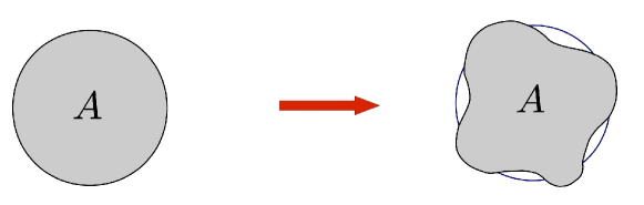
Figure 1: Shape deformation of the droplet under the action of area preserving diffeomorphisms.

We can generate the deformed droplets by coordinate transformations of the plane that keep the area constant: these are the so-called two-dimensional area-preserving diffeomorphisms [19][20]. Their action can be expressed in terms of Poisson brackets, in analogy with canonical transformations of a two-dimensional phase space. It is convenient to use complex coordinates of the plane,

$$z=x^{1}+ix^{2},\qquad\bar{z}=x^{1}-ix^{2},\qquad ds^{2}=dzd\bar{z},\qquad\delta_{z\bar{z}}=\frac{1}{2},\qquad\delta^{z\bar{z}}=2.$$ (2.1)

The Poisson brackets are:

$$\{f,g\}=\varepsilon^{z\bar{z}}\partial_{z}f\;\partial_{\bar{z}}g+\varepsilon^{\bar{z}z}\partial_{\bar{z}}f\;\partial_{z}g,\qquad\varepsilon^{z\bar{z}}=-\varepsilon^{\bar{z}z}=-2i.$$ (2.2)

The area-preserving transformations are given by,

$$\delta_{w}z=\{z,w(z,\bar{z})\},$$ (2.3)

in terms of the generating function $w(z,\bar{z})$. The deformations of the ground-state density $\rho_{GS}$ follows from the chain rule:

$$\rho_{GS}=\rho_{o}\Theta\left(R^{2}-z\bar{z}\right),\qquad\delta_{w}\rho_{GS}=\{\rho,w\}\propto\delta\left(z\bar{z}-R^{2}\right),$$ (2.4)

where $\Theta$ is the step function. We see that fluctuations have support at the boundary $\bar{z}z=R^{2}$, as expected.

A basis of generators can be obtained by expanding the function $w(z,\bar{z})$ in power series,

$$\mathcal{L}_{n,m}=z^{n+1}\bar{z}^{m+1},\qquad w(z,\bar{z})=\sum_{n,m\geq-1}c_{nm}z^{n+1}\bar{z}^{m+1}.$$ (2.5)

These generators obey the following algebra:

$$\left\{\mathcal{L}_{n,m},\mathcal{L}_{k,l}\right\}=\left[\left(m+1\right)\left(k+1\right)-\left(n+1\right)\left(l+1\right)\right]\mathcal{L}_{n+k,m+l},$$ (2.6)

that is called the $w_{\infty}$ algebra of classical area-preserving diffeomorphisms.

We now consider the realization of this symmetry in the quantum Hall effect, starting from the lowest Landau level for simplicity [19]. In the quantum theory, the generators (2.5) become one-body operators,

$$\hat{\mathcal{L}}_{n,m}=\int d^{2}z\ \hat{\Psi}^{\dagger}(z,\bar{z})\ \bar{z}^{m+1}z^{n+1}\ \hat{\Psi}(z,\bar{z}),\qquad n,m\geq-1,$$ (2.7)

where the field operator $\hat{\Psi}(z,\bar{z})$ is,

$$\hat{\Psi}(z,\bar{z})=e^{-z\bar{z}/2\ell^{2}}\ \hat{\varphi}(z),\qquad\hat{\varphi}(z)=\frac{1}{\ell\sqrt{\pi}}\sum_{n=0}^{\infty}\left(\frac{z}{\ell}\right)^{n}\frac{1}{\sqrt{n!}}\ \hat{c}_{n},\qquad\{\hat{c}_{n},\hat{c}^{\dagger}_{m}\}=\delta_{n,m}.$$ (2.8)

In this expression, there appear the analytic field $\hat{\varphi}(z)$, the fermionic creation-annihilation operators, $\hat{c}_{n},\hat{c}^{\dagger}_{m}$, and the magnetic length $\ell=\sqrt{2\hbar/B}$. We set $\ell=1$ in the following, unless when specified.

The coordinates become non-commuting, $[\bar{z},z]=\ell^{2}$, when acting on analytic fields $\hat{\varphi}(z)$, and classical polynomials in $z,\bar{z}$ require a choice of normal ordering. The definition of $\hat{\mathcal{L}}_{n,m}$ in (2.7) adopts the standard prescription, setting $\bar{z}$ to the left of $z$ and then replacing $\bar{z}\to\ell^{2}\partial_{z}$, the holomorphic derivative. Other normal-ordering choices are possible: in the following, it is convenient to consider the case of anti-normal ordering, placing $\bar{z}$ to the right of $z$. In this case, the generators read:

$$\hat{\mathcal{L}}_{n,m} = \int d^{2}z\ e^{-z\bar{z}/\ell^{2}}\ \hat{\varphi}^{\dagger}(z)\ z^{n+1}\left(\ell^{2}\partial_{z}\right)^{m+1}\hat{\varphi}(z)$$ (2.9)

$$= \ell^{n+m+2}\sum_{k\geq 1}\frac{\sqrt{(k+m)!(k+n)!}}{(k-1)!}\ c^{\dagger}_{k+n}c_{k+m}.$$

The Fock-space expression is useful to derive the following commutation relations,

$$\left[\hat{\mathcal{L}}_{n,m},\hat{\mathcal{L}}_{k,l}\right]=\sum_{s=1}^{Min(m,k)} \frac{\ell^{2s}\ \left(m+1\right)!\left(k+1\right)!}{\left(m-s+1\right)!\left(k-s+1\right)!s!}\hat{\mathcal{L}}_{n+k-s+1,m+l-s+1}$$ (2.10)

$$-\left(m\leftrightarrow l,n\leftrightarrow k\right),$$

that are called the $W_{\infty}$ algebra of quantum area-preserving transformations.

Let us discuss a number of properties of this algebra [19].

• On the right hand side there occur a finite number of terms involving increasing powers of $\ell^{2}=2\hslash/B$; the first term corresponds to the quantization of the classical algebra (2.6), the others are higher-order quantum corrections; their form changes for other normal-orderings of $\hat{\mathcal{L}}_{n,m}$.

• The $W_{\infty}$ algebra contains an infinite number of Casimir invariants, the operators $\hat{\mathcal{L}}_{n,n}$ that actually correspond to radial moments $O(r^{2n+2})$ of the density (cf. (2.7)). In particular $\hat{\mathcal{L}}_{0,0}=z\partial_{z}$ is the angular momentum operator and obeys the algebra:

  $$\left[\hat{\mathcal{L}}_{0,0},\hat{\mathcal{L}}_{n,m}\right]=(n-m)\hat{\mathcal{L}}_{n,m}.$$ (2.11)

• It is apparent from the second-quantized expression (2.9) that the $\hat{\mathcal{L}}_{n,m}$ create bosonic particle-hole excitations with angular momentum jump $\Delta k=n-m$, whose amplitude is parameterized by another integer, say $m$.

• Area-preserving diffeomorphisms can be similarly implemented in the higher Landau levels, by replacing the corresponding field operators in (2.7). Actually, the transformations act within each level. The second quantized expression (2.9) is valid for any level by just replacing the corresponding creation-annihilation operators [19].

• The $W_{\infty}$ algebra can be written in another basis by expressing the generating function (2.5) in terms of plane waves, $w_{k,\bar{k}}(z,\bar{z})=\exp(ik\bar{z}/2+i\bar{k}z/2)$. Owing to Eq.(2.7), the corresponding quantum generators become the Fourier modes of the density $\hat{\rho}(k,\bar{k})$, obeying the Girvin-MacDonald-Platzman algebra [26]:

  $$\left[\hat{\rho}(k,\bar{k}),\hat{\rho}(p,\bar{p})\right]=\left(e^{p\bar{k}/4}-e^{\bar{p}k/4}\right)\hat{\rho}(k+p,\bar{k}+\bar{p}).$$ (2.12)

  It is apparent that the $\hat{\rho}(k,\bar{k})$ corresponds to the generating function of polynomial operators $\hat{\mathcal{L}}_{n,m}$ (in the so-called Weyl ordering, e.g. $z\bar{z}\to(z\partial/\partial z+\partial/\partial z\;z)/2$). The Fourier basis is better known in the literature, but the polynomial basis is more convenient for the following discussion of excitations.

Let us now find the action of $W_{\infty}$ generators on the ground state. Consider the lowers Landau level completely filled by $N$ electrons. Its second quantized expression is:

$$|\Omega\rangle=|N,\nu=1\rangle=c^{\dagger}_{N-1}c^{\dagger}_{N-2}\cdots c^{\dagger}_{1}c^{\dagger}_{0}|0\rangle.$$ (2.13)

Being a completely filled Fermi sea, this state does not admit particle-hole transitions decreasing the total angular momentum, that are generated by $\hat{\mathcal{L}}_{n,m}$ with $\Delta k=n-m<0$, see Eq.(2.9). It then follows that the ground state obeys the following conditions:

$$\hat{\mathcal{L}}_{n,m}|\Omega\rangle=0,\qquad{\rm for}\qquad-1\leq n<m.$$ (2.14)

These are called highest-weight conditions, borrowing the language of infinite-dimensional algebra representations [29]. The highest-weight state is the top (or bottom) state of an infinite tower, and is annihilated by half of the ladder operators.

The action of the other $W_{\infty}$ generators is the following. The Casimirs leave the ground state invariant and possess eigenvalues that are polynomials in $N$. For example, the operators,

$$\hat{\mathcal{L}}_{-1,-1}|\Omega\rangle=N|\Omega\rangle,\qquad\hat{\mathcal{L}}_{0,0}|\Omega\rangle=\frac{N(N-1)}{2}|\Omega\rangle,$$ (2.15)

respectively measure the number of particles and the angular momentum.

The $W_{\infty}$ generators with $\Delta k=n-m>0$ increase the angular momentum and create excitations:

$$\hat{\mathcal{L}}_{n,m}|\Omega\rangle=|{\rm excit}\rangle,\qquad{\rm for}\qquad n>m\geq-1.$$ (2.16)

Actually, it can be shown that they generate the entire space of neutral excitations in the lowest Landau level, because the relation (2.9) between $\hat{\mathcal{L}}_{n,m}$ and fermionic bilinears is invertible. These generators provide a kind of non-relativistic bosonization of Hall electrons [19].

In conclusion, we have shown that the $W_{\infty}$ transformations are spectrum-generating, i.e. correspond to the dynamical symmetry of the $\nu=1$ quantum Hall system. Let us add some remarks.

• As is well known, the algebraic approach of dynamical symmetries is only useful when the Hamiltonian can be simply written in terms of the generators. Later we shall see that short-range two-body interactions can indeed be included. So far, we only considered free electrons in a confining potential: a quadratic form $V(z,\bar{z})=\lambda\bar{z}z$ actually corresponds to the generator $\hat{\mathcal{L}}_{0,0}$ with simple commutation relations (2.11).

• Different normal orderings of the $W_{\infty}$ generators amount to redefinitions,

  $$\hat{\mathcal{L}}_{n,m}\quad\longrightarrow\quad\hat{\mathcal{L}}_{n,m}+a\hat{\mathcal{L}}_{n-1,m-1}+b\hat{\mathcal{L}}_{n-2,m-2}+\cdots,$$ (2.17)

  where $a,b,\cdots$ are numerical constants, as easily seen by Eq.(2.7). It follows that the ground-state conditions (2.14) are valid for any choice of normal ordering.

2.2 W-infinity symmetry of Laughlin states

The Laughlin ground states with fillings $\nu=1/(2s+1)=1/3,1/5,\dots$ are better discussed in coordinate representation. Let us rewrite the $W_{\infty}$ generators introduced earlier for $\nu=1$ in terms of the electron coordinates $z_{i}$, $i=1,\dots,N$. They read,

$$\hat{\mathcal{L}}_{n,m}=\sum_{i=1}^{N}z_{i}^{n+1}\;\partial_{z_{i}}^{m+1}.$$ (2.18)

The (analytic part of the) ground state wave function is written

$$\Psi_{1}(z_{1},\dots,z_{N})=\Delta\left(\left\{z_{i}\right\}\right),\qquad\quad\Delta\left(\left\{z_{i}\right\}\right)=\prod_{1=i<j=N}\left(z_{i}-z_{j}\right),$$ (2.19)

in terms of the Vandermonde determinant.

The $W_{\infty}$ highest-weight conditions (2.14) are rewritten:

$$\hat{\mathcal{L}}_{n,m}\Psi_{1}=\sum_{i=1}^{N}z_{i}^{n+1}\;\partial_{z_{i}}^{m+1}\prod_{1=i<j=N}\left(z_{i}-z_{j}\right)=0,\qquad-1\leq n<m.$$ (2.20)

Note that these conditions are not completely trivial in terms of coordinates and actually involve some polynomial identities.

We now define new $W_{\infty}$ generators that fulfill the same highest-weight conditions when acting on Laughlin states. The Laughlin wavefunction reads,

$$\Psi_{2s+1}(z_{1},\dots,z_{N})=\Delta\left(\left\{z_{i}\right\}\right)^{2s+1},\qquad\quad\nu=\frac{1}{2s+1}.$$ (2.21)

We modify the $W_{\infty}$ generators by performing the similarity transformation [30],

$$\hat{\mathcal{L}}_{n,m}^{(1)}\qquad\longrightarrow\qquad\hat{\mathcal{L}}_{n,m}^{(2s+1)} = \Delta\left(\left\{z_{i}\right\}\right)^{2s}\ \hat{\mathcal{L}}_{n,m}^{(1)}\ \Delta\left(\left\{z_{i}\right\}\right)^{-2s}$$ (2.22)

$$= \sum_{i=1}^{N}z_{i}^{n+1}\left(\partial_{z_{i}}-\sum_{j,j\neq i}\frac{2s}{z_{i}-z_{j}}\right)^{m+1}.$$

The new generators $\hat{\mathcal{L}}_{n,m}^{(2s+1)}$ clearly obey the highest-weight conditions (2.14) on Laughlin wavefunctions: for $n<m$, they cannot compress it (although some other operators could); for $n>m$, they generate particle-hole excitations above this state.

Other nice features are:

• The operators (2.22) fulfill the same $W_{\infty}$ algebra (2.10), owing to the similarity transformation. As discussed in Ref.[30], this rather singular transformation may lead to non-holomorphic delta-function singularities, but these are irrelevant in expectation values, due to the zeroes of wavefunctions.

• It can be shown that the modified derivatives in (2.22) are actually arising by coupling electrons to a Chern-Simons statistical field with coupling constant $1/2s$, that “attaches and even number of flux quanta to electrons” [10]. Therefore the similarity transformation (2.22) is actually the Jain composite-fermion map between integer and Laughlin Hall states [7].

2.3 $W_{\infty}$ symmetry of edge excitations

The results of the previous sections can be summarized by saying that integer and fractional Hall states possess the dynamical symmetry of quantum area-preserving diffeomorphisms. Given that these generators span the space of excitations, they should account for both bulk and edge properties of the quantum incompressible fluid.

However, few results were obtained in this general setting because the $W_{\infty}$ generators are too singular in the $N\to\infty$ limit of large droplets, that is relevant for universal features. The eigenvalues of the Casimirs (2.15) grow polynomially in $N$, the Fock space expression (2.9) and the covariant derivatives (2.22) require regularization and renormalization. As a consequence, the $W_{\infty}$ algebra (2.10) does not have a finite large $N$ limit and its renormalized form was not understood so far.

Fortunately, it was found that a well-defined formulation of the $W_{\infty}$ symmetry exists in the Hilbert space of $(1+1)$-dimensional massless field theories, that describe the edge excitations of the Hall droplet [21]. In this setting, $W_{\infty}$ is an extension of the conformal symmetry and the corresponding representations were completely understood in the mathematical literature [31]. The $W_{\infty}$ algebra on the circle edge has a well defined large $N$ limit, where it acquires a unique central extension, corresponding to the conformal anomaly [29].

Therefore, the works [21][27] proposed to study the $W_{\infty}$ symmetry directly in the edge theory and to understand its implications for the conformal field theory description.

The edge excitations of the filled lowest Landau level are described by a massless chiral (Weyl) fermion in one dimension [32]: both theories possess the same one-component fermionic Fock space, but amplitudes and measure of integration are different. The edge is identified as the circle $C_{R}$, $z=R\exp(i\theta)$, and the radial dependence is lost. The earlier quantization (2.7) of $w_{\infty}$ generators is replaced by the following expression:

$$\hat{\mathcal{L}}_{n+i,i}\quad\longrightarrow\quad-\hat{V}_{-n}^{(i+2)}=\oint_{C_{R}}\frac{dz}{iz}\ \hat{\psi}^{\dagger}(z)\ z^{n}\left(z\partial_{z}\right)^{i+1}\hat{\psi}(z),$$ (2.23)

involving the Weyl fermion field,

$$\hat{\psi}(z)=\frac{1}{\sqrt{2\pi}}\sum_{k=-\infty}^{\infty}z^{k-1/2}\ \hat{c}_{k},\qquad\left\{\hat{c}_{n},\hat{c}^{\dagger}_{m}\right\}=\delta_{n,m}.$$ (2.24)

Note that $z\partial_{z}\to-i\partial/\partial\theta$ on the circle and that the $N$ dependence has disappeared.

Therefore, the $W_{\infty}$ algebra on the circle is different from (2.10), with the exception of the leading $O(\hbar)$ term. Nevertheless, it still contains infinite Casimirs $\hat{V}^{(i)}_{0}$, $i=0,1,2,\dots$ that correspond to conserved charges in the conformal theory. The operators $\hat{V}_{n}^{(1)}$ are identified as the modes $\hat{\rho}_{n}$ of the edge density $\hat{\rho}(z)$ in the Weyl theory, while $\hat{V}_{n}^{(2)}$ are the Virasoro operator $\hat{L}_{n}$ [21]. Their algebra reads (omitting the hats on operators hereafter):

$$\left[\rho_{n},\rho_{m}\right]=n\delta_{n+m,0},$$ (2.25)

$$\left[L_{n},\rho_{m}\right]=-m\rho_{n+m},$$

$$\left[L_{n},L_{m}\right]=(n-m)L_{n+m}+\frac{c}{12}n\left(n^{2}-1\right)\delta_{n+m,0},$$ (2.26)

where $c$ is the Virasoro central charge ($c=1$ for the Weyl fermion). The algebra obeyed by higher-spin operators can be found in [28].

The ground state relations (2.14) obeyed by the $W_{\infty}$ generators are mapped in the highest weight conditions of conformal representations, such as [21]:

$$\rho_{k}|\Omega\rangle=0,\qquad L_{k}|\Omega\rangle=0,\qquad k\geq 0.$$ (2.27)

The physical implications of the $W_{\infty}$ symmetry have been investigated for general edge theories beside the Weyl fermion pertaining to $\nu=1$: here we summarize the results.

• In the simplest case, $W_{\infty}$ is the enveloping algebra of the current algebra with central charge $c=1$: namely, the higher-spin currents correspond to polynomials of the edge density $\rho(z)$, generalizing the so-called Sugawara construction: $V^{(1)}(z)=\rho(z)$, $V^{(2)}=:\rho(z)^{2}:$, $V^{(3)}=:\rho(z)^{3}:$, etc [21]. One recovers the chiral Luttinger theory (compactified chiral boson) of Laughlin edge states. The higher-spin currents are automatically implemented without any further condition on the conformal theory.

• The description of edge excitations for the Jain states with $\nu=n/(2sn\pm 1)$ is based on the $n$-component current algebra with central charge $c=n$, whose spectrum is parameterized by an integer-valued symmetric matrix, called $K$ matrix. The specific form of $K$ describing Jain states is obtained from simple phenomenological arguments based on the composite fermion map. General $W_{\infty}$ representations also correspond to current algebras with $c=n$: however, there is a fine structure that allows to identify “minimal models” of $W_{\infty}$ symmetry, possessing a reduced set of excitations [27]. These models realize the $U(1)\times SU(n)_{1}$ extended symmetry and precisely select the $K$ matrix for Jain states. Therefore, the $W_{\infty}$ symmetry and the requirement of minimality are sufficient to a-priori identify the Jain states without any phenomenological input. This purely geometric characterization of the prominent Hall states is rather remarkable.

• The non-Abelian Hall states, such as the Pfaffian with central charge $c=3/2$, cannot directly be identified among $W_{\infty}$ symmetric theories. The explanation of this fact is the that additional features are present. In the case of the Pfaffian, this is the electron pairing mechanism, leading to the incompressible fluid of bosonic compounds. In the works [33], this pairing was described by a projection in a two-fluid $c=2$ model that possess the $W_{\infty}$ symmetry. This description of the Pfaffian by an Abelian “parent” state brings back in the $W_{\infty}$ symmetry and also implies some useful relations for wavefunction modeling.

• While the lower Casimirs $\rho_{0}$ and $L_{0}$ respectively express the charge and Hamiltonian $H=vL_{0}/R$ of edge excitations, the higher ones encode non-relativistic corrections $\Delta H^{(i)}=V^{(i)}_{0}/R^{i-1}$, $i=3,4,\dots,$ to the energy spectrum, forming a series in $1/R$.

In conclusion, the $W_{\infty}$ symmetry of quantum incompressible fluids has definite implications for edge theories. On the contrary, bulk excitations were not much investigated beyond the rather formal results presented in Section 2.1 and 2.2. In particular, the map (2.23) between the bulk operators ${\mathcal{L}}_{n,m}$ (for a given normal ordering) and the edge generators $V_{n}^{(i)}$ was unclear.

3 Radial shape of edge excitations

3.1 Laplace transform and bulk-boundary map

A first understanding of the bulk-boundary map was obtained only recently, by a more careful definition of the edge limit [22] (See also [34]). It was shown that the modes of the edge current $\rho_{n}$ are simply obtained by integrating out the radial dependence of the bulk density,

$$\rho_{m}=\int_{0}^{\infty}drr\int_{0}^{2\pi}d\theta\;\rho(r,\theta)e^{-im\theta},$$ (3.1)

and by taking the limit $R\to\infty$ for values of coordinate $r$ and angular momentum $m$ at the edge of the droplet, as follows:

$$r=R+x,\qquad|x|<1,\qquad m=R^{2}+m^{\prime},\qquad|m^{\prime}|<R,\qquad R\to\infty.$$ (3.2)

In this limit, the $\rho_{n}$ become operators in the edge conformal theory and obey the expected current algebra commutation relations, $\left[\rho_{n},\rho_{m}\right]=n\delta_{n+m,0}$.

In this Section, we are going to extend this map to higher-spin $W_{\infty}$ generators and the full algebra, thus clearly establishing the link between bulk and edge descriptions. Furthermore, in Section four this setup will allow us to go beyond the conformal theory description.

The key idea is to consider the Laplace transform of the bulk density with respect to $r^{2}$:

$$\rho_{k}(\lambda)=\int_{0}^{\infty}drre^{-\lambda r^{2}}\int_{0}^{2\pi}d\theta\;\hat{\rho}(r,\theta)e^{-ik\theta}.$$ (3.3)

Expanding the field operators (2.8) in the Fock basis, we find:

$$\rho_{k}(\lambda)=\sum_{j=0}^{\infty}\frac{1}{(1+\lambda)^{j+1+k/2}}\frac{\Gamma\left(j+1+\frac{k}{2}\right)}{\left(\Gamma(j+1)\Gamma(j+k+1)\right)^{1/2}}c^{\dagger}_{j}c_{j+k}.$$ (3.4)

It turns out that this quantity possesses a finite $R\to\infty$ limit, up to a multiplicative factor. Taking the limit according to (3.2), we obtain,

$$\rho_{k}(\lambda)=\frac{1}{\left(1+\lambda\right)^{R^{2}+\mu+1}}\sum_{j^{\prime}=-R^{2}}^{\infty}(1+\lambda)^{\mu-j^{\prime}-k/2}:c_{j^{\prime}}^{\dagger}c_{j^{\prime}+k}:,\qquad R\to\infty.$$ (3.5)

Upon removing the prefactor, $(1+\lambda)^{-R^{2}-\mu-1}$, we obtain a well-defined quantity in the Weyl-fermion edge theory (2.24):

$$\rho_{k}(\lambda)\ \longrightarrow\ \sum_{j^{\prime}=-R^{2}}^{\infty}(1+\lambda)^{\mu-j^{\prime}-k/2}:c_{j^{\prime}}^{\dagger}c_{j^{\prime}+k}:.$$ (3.6)

In these expression, we also introduced the chemical potential $\mu$ that should take the value $1/2$ for standard Neveu-Schwarz boundary conditions on the circle, and the normal ordering, $:(\ \ ):$, for regularizing the infinite Dirac sea. This is defined by the ground-state conditions,

$$\begin{array}[]{l}c_{k}|\Omega\rangle=0,\quad k>0,\\ c_{k}^{\dagger}|\Omega\rangle=0,\quad k\leq 0,\end{array}\qquad:c^{\dagger}_{k}c_{k}:=\left\{\begin{array}[]{l}\ \ c^{\dagger}_{k}c_{k},\quad k>0,\\ -c_{k}c_{k}^{\dagger},\quad k\leq 0.\end{array}\right.$$ (3.7)

Note that the Laplace-transformed density (3.3) is by definition the generating function of $W_{\infty}$ operators (2.7) in the bulk; after regularization, it accounts for the edge operators,

$$\rho_{k}(\lambda)=\rho_{k}-\lambda L_{k}+\frac{\lambda^{2}}{2}V^{(3)}_{k}+\cdots,$$ (3.8)

as defined in (2.23). The $R\to\infty$ subtractions (polynomial in $R^{2}=N-1$) are rather remarkably accounted for. For example, the ground-state values [32],

$$\rho_{0}|\Omega\rangle=\left(\frac{1}{2}-\mu\right)|\Omega\rangle,\qquad\quad L_{0}|\Omega\rangle=\frac{1}{2}\left(\frac{1}{2}-\mu\right)^{2}|\Omega\rangle,\qquad\left(\mu\to\frac{1}{2}\right),$$ (3.9)

should be contrasted with the bulk values (2.15) of order $N$ and $N^{2}$, respectively. Therefore, the Laplace transformed density is the convenient quantity to establish the bulk-boundary correspondence.

We can now compute the algebra obeyed by the regularized generators (3.6) by using Fock space expressions. The result is:

$$\left[\rho_{k}(\lambda),\rho_{n}(\mu)\right]=\left(t^{-\frac{n}{2}}y^{\frac{k}{2}}-t^{\frac{n}{2}}y^{-\frac{k}{2}}\right)\rho_{k+n}(\eta)+c\;\delta_{k+n,0}\frac{z^{\frac{k}{2}}-z^{-\frac{k}{2}}}{z^{\frac{1}{2}}-z^{-\frac{1}{2}}},$$ (3.10)

where

$$t=\frac{1}{1+\lambda},\qquad y=\frac{1}{1+\delta},\qquad z=ty=\frac{1}{1+\eta}.$$ (3.11)

This is again the $W_{\infty}$ algebra (2.10) written in a basis that makes it clear the map between the bulk and the edge: it is expressed in terms of bulk operators but it realizes explicitly the conformal theory representation. There appears the central extension proportional to $c\;\delta_{k+n,0}$, $c=1$, that originates from normal ordering. Upon expanding (3.10) in series of $\lambda$ and $\delta$, and comparing with (3.8) one recovers the standard current algebra relations (2.26). The highest-weight conditions are:

$$\rho_{k}(\lambda)|\Omega\rangle=0,\qquad\quad k\geq 0,\qquad\forall\lambda,$$ (3.12)

because they hold for any current in the expansion (3.8).

3.2 Radial shape of neutral excitations

A particle-hole excitation is described by the state $|\{k\}\rangle=\rho_{-k}|\Omega\rangle$, with momentum $k>0$. The density fluctuation can be obtained from the expectation value,

$$\langle\rho_{0}(\lambda)\rangle_{\{k\}}=\frac{\langle\{k\}|\rho_{0}(\lambda)|\{k\}\rangle}{\langle\{k\}|\{k\}\rangle}=\frac{\langle\Omega|\left[\rho_{k}(0),[\rho_{0}(\lambda),\rho_{-k}(0)]\right]|\Omega\rangle}{\langle\Omega|\left[\rho_{k}(0),\rho_{-k}(0)\right]|\Omega\rangle},\qquad k>0,$$ (3.13)

that determines the radial profile by inverse Laplace transform.

Expression (3.13) is computed by using the algebra (3.10). After restating the prefactor in (3.5), one finds the result:

$$\langle\rho_{0}(\lambda)\rangle_{\{k\}}=-\frac{\left(1-(1+\lambda)^{k}\right)^{2}}{k\lambda(1+\lambda)^{R^{2}+k+1}}.$$ (3.14)

This quantity only contains poles, since $R^{2}=N-1$, and its inverse Laplace transform is computed by taking a path parallel to the imaginary $\lambda$ axis and located to the right of all singularities, as usual. Details of the calculation are given in the Appendix. One finds the following expression in the edge limit (3.2):

$$\langle\delta\rho(r)\rangle=\frac{1}{\pi}\langle\delta\rho_{0}(r^{2})\rangle_{\{k\}}=\frac{4kx}{R^{2}}\frac{e^{-2x^{2}}}{(2\pi)^{3/2}},\qquad r=R+x,\quad|x|<1.$$ (3.15)

Of course, this result could have been directly obtained by using fermionic Fock space. The expectation value over particle-hole fluctuations reads:

$$\langle\delta\rho(r)\rangle_{\{k\}}=\sum_{m^{\prime}}\left|\phi_{R^{2}+m^{\prime}}\right|^{2}\langle:c^{\dagger}_{m^{\prime}}c_{m^{\prime}}:\rangle_{\{k\}}=\frac{1}{k}\left(\sum_{i=1}^{k}\left|\phi_{R^{2}+i}\right|^{2}-\left|\phi_{R^{2}+i-k}\right|^{2}\right).$$ (3.16)

This quantity matches (3.15) upon using the expression of wavefunctions (2.8) in the limit to the edge [22],

$$\phi_{R^{2}+m^{\prime}}(r,\theta)\sim\left(\frac{2}{\pi}\right)^{1/4}\frac{e^{i(R^{2}+m^{\prime})\theta}}{\sqrt{2\pi R}}e^{-\left(x-\frac{m^{\prime}}{2R}\right)^{2}}.$$ (3.17)

The comparison provides a check for the previous analysis of the edge limit. The advantage of the $W_{\infty}$ bosonic approach is that it can be straightforwardly extended to fractional Hall states, as described in Section 3.4.

The density fluctuation (3.15) is plotted in Fig.2 together with the ground state profile near the edge. One remarks the small size, $O(1/R^{2})$ w.r.t. to the $O(1)$ ground state, and the support over $|x|=O(1)$.

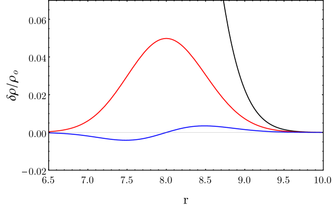
Figure 2: Radial density profile of $\nu=1$ ground state near the edge (normalized to one in the bulk, black line); $k=1$ particle-hole excitation (blue); $Q=1$ charged edge excitation (red) (for $N=64$ electrons).

3.3 Shape of charged excitations

The profile of a charged excitation at the edge can be obtained by following similar steps. The corresponding state is $|Q\rangle=V_{Q}(0)|\Omega\rangle$, where $V_{Q}(z)$ is the vertex operator of charge $Q$ in the $c=1$ conformal theory. The charged state is the highest-weight state of another representation of the algebra and obeys the conditions,

$$\rho_{k}(\lambda)|Q\rangle=0,\qquad\quad\ k>0,\qquad\forall\lambda,$$ (3.18)

$$\rho_{0}|Q\rangle=Q|Q\rangle,\qquad\quad L_{0}|Q\rangle=\frac{Q^{2}}{2}|Q\rangle,$$ (3.19)

analogous to those of the ground state (3.9) and (3.12), respectively.

The zero mode of the Laplace-transformed density, $\rho_{0}(\lambda)$ is actually the generating function of all higher-spin Casimirs, whose eigenvalues are known from the study of $W_{\infty}$ representations by the authors of Ref. [31]. We need to perform a change of parameters for interpreting their result: the $W_{\infty}$ operators were presented in the form $V\left(z^{k}\exp(az\partial_{z})\right)$, being the generating function of higher-spin operators (cf. (2.23)). Their value on charged states was found to be,

$$V\left(z^{k}e^{az\partial_{z}}\right)|Q\rangle=\frac{e^{aQ}-1}{e^{a}-1}|Q\rangle,$$ (3.20)

and the corresponding algebra was written,

$$\left[V\left(z^{k}e^{az\partial_{z}}\right),V\left(z^{n}e^{bz\partial_{z}}\right)\right]=\left(e^{an}-e^{bk}\right)V\left(z^{k+n}e^{(a+b)z\partial_{z}}\right)+c\;\delta_{k+n,0}\frac{e^{-ak}-e^{bk}}{1-e^{a+b}},$$ (3.21)

($c=1$ here). These generators differ by our $\rho_{k}(\lambda)$ in the ordering of derivatives. The comparison of the two algebras, (3.10) and (3.21), and the known data (3.19) allows to find the relation between the two parameterizations, with the result:

$$V\left(z^{-k}e^{az\partial_{z}}\right)\equiv e^{a(k-1)/2}\rho_{k}(\lambda),\qquad\qquad e^{a}=\frac{1}{1+\lambda}.$$ (3.22)

The density profile for charged excitations is given by the expectation value $\langle Q|\rho_{0}(\lambda)|Q\rangle$. Upon using (3.20)) with the identifications (3.22), we obtain:

$$\langle\rho_{0}(\lambda)\rangle_{Q}=\frac{\langle Q|\rho_{0}(\lambda)|Q\rangle}{\langle Q|Q\rangle}=\frac{1-(1+\lambda)^{-Q}}{(1+\lambda)^{1/2}-(1+\lambda)^{-1/2}}.$$ (3.23)

The inverse Laplace transform of the expression (3.23) after inclusion of the bulk prefactor $1/(1+\lambda)^{R^{2}+3/2}$, leads to the result (see the Appendix):

$$\langle\delta\rho(r)\rangle_{Q}=\frac{1}{\pi}\langle\rho_{0}(r^{2})\rangle_{Q}=\frac{e^{-r^{2}}}{\pi}\sum_{n=N}^{N+Q-1}\frac{r^{2n}}{\Gamma(n+1)}.$$ (3.24)

In the $\nu=1$ case, this expression is rather simple, owing to the integer values of $R^{2}=N-1$ and $Q$: one recovers the sum of squared wavefunctions for $Q$ electrons added at the edge. This result is actually exact, in spite of the approximations made in the limit to the edge. Upon using the edge limit of wavefunctions (3.17), we obtain the expression:

$$\langle\delta\rho(r)\rangle_{Q}=\left(\frac{2}{\pi}\right)^{1/2}\frac{e^{-2x^{2}}}{2\pi R}Q+O\left(\frac{1}{R^{2}}\right),\qquad r=R+x,\quad|x|<1.$$ (3.25)

This fluctuation is definite positive, of size $O(1/R)$ and still localized in a region of one magnetic length at the edge (see Fig.2).

In conclusion, we have shown that the study of the $W_{\infty}$ symmetry in the edge conformal field theory is able to describe the radial shape of excitations, that is actually a two-dimensional property of incompressible fluids. This kind of dimensional extension is possible thanks to the existence of an infinite tower of conserved currents. In the discussion of Section two, we said that the radial dependence is lost in the limit to the edge, but this is not actually true.

3.4 Density profiles for Laughlin states

The $W_{\infty}$ symmetry description of edge excitations extends to Laughlin states with filling fractions $\nu=1/m=1/3,1/5,\dots$. The algebra (3.10) of $\rho_{k}(\lambda)$ is unchanged but the representations are different: the generating function of Casimirs (3.23) takes the same form, but the charge $Q$ is no longer integer quantized.

As explained in Section 2, the $W_{\infty}$ algebra with central charge $c=1$ contains the current algebra (2.26) of charge and angular momentum operators, that has been extensively analyzed for Laughlin states [32]. Their eigenstates have been determined by e.g. canonical quantization of the chiral boson theory, and read:

$$\rho_{0}|\frac{n}{m}\rangle=\frac{n}{\sqrt{m}}|\frac{n}{m}\rangle,\qquad L_{0}|\frac{n}{m}\rangle=\frac{n^{2}}{2m}|\frac{n}{m}\rangle,\qquad\ \ n\in\mathbb{Z},\quad\left(\nu=\frac{1}{m}\right).$$ (3.26)

Note that the physical charge is $Q=n/m$, but the eigenvalue $\widetilde{Q}=n/\sqrt{m}$ of $\rho_{0}$ differs by a proportionality factor due to our normalization of the current algebra (2.26).

As explained in the previous section, the Laplace transformed density for charged excitations is obtained from the generating function of Casimirs, Eq.(3.23). After inclusion of the bulk prefactor, it reads:

$$\langle\widetilde{\rho}_{0}(\widetilde{\lambda})\rangle_{\widetilde{Q}}=\frac{1-(1+\widetilde{\lambda})^{-\widetilde{Q}}}{\widetilde{\lambda}(1+\widetilde{\lambda})^{\widetilde{R}^{2}+1}}\sim\widetilde{Q}-\widetilde{\lambda}\left(\frac{\widetilde{Q}^{2}}{2}+\widetilde{Q}\left(\widetilde{R}^{2}+\frac{3}{2}\right)\right)+O(\widetilde{\lambda}^{2}).$$ (3.27)

The first two terms in the expansion in $\widetilde{\lambda}$ specify the edge charge $\rho_{0}$ and angular momentum $L_{0}$ eigenvalues. Using the spectrum (3.26), we find the following result for the excitation of $q$ electrons added at the boundary,

$$\langle\widetilde{\rho}_{0}(\widetilde{\lambda})\rangle_{\widetilde{Q}}\sim\sqrt{m}q-\widetilde{\lambda}\left(\frac{mq^{2}}{2}+q\sqrt{m}\left(\widetilde{R}^{2}+\frac{3}{2}\right)\right)+O(\widetilde{\lambda}^{2}).$$ (3.28)

This expression should be compared with the approximate knowledge of bulk data for fractional fillings. The first two moments of the density, in presence of $q$ added electrons, are:

$$\int d^{2}r\left(\rho_{N+q}(r)-\rho_{N}(r)\right)=q,$$

$$\int d^{2}r\;r^{2}\left(\rho_{N+q}(r)-\rho_{N}(r)\right)=\frac{m}{2}\left(q^{2}+2q\left(N+O(1)\right)\right).$$ (3.29)

where the term $O(1)$ as $N\to\infty$ depend on the form of the electron droplet near the edge, that is not relevant in the present discussion (The ground state profile will be analyzed in the next Section). Therefore, we can infer the bulk expression:

$$\langle\rho_{0}(\lambda)\rangle_{q}\sim q-\lambda\left(\frac{mq^{2}}{2}+q\left(mN+O(1)\right)\right)+O(\lambda^{2}),$$ (3.30)

where $R^{2}=mN+O(1)$ for $N\to\infty$. The comparison of edge (3.28) and bulk (3.30) results leads to the following identification of parameters,

$$\rho_{0}(\lambda)=\frac{\widetilde{\rho}_{0}(\widetilde{\lambda})}{\sqrt{m}},\qquad\widetilde{\lambda}=\sqrt{m}\lambda,\qquad\widetilde{R}^{2}=\frac{R^{2}}{\sqrt{m}}.$$ (3.31)

After the matching, the density of charged excitations is finally found to be:

$$\langle\rho_{0}(\lambda)\rangle_{Q}=\frac{1}{m}\;\frac{1-(1+\sqrt{m}\lambda)^{-\frac{n}{\sqrt{m}}}}{\lambda(1+\sqrt{m}\lambda)^{\frac{R^{2}}{\sqrt{m}}}},\qquad\quad Q=\frac{n}{m},\quad\nu=\frac{1}{m}.$$ (3.32)

The inverse Laplace transform determines the following radial profile (see Appendix for the derivation),

$$\langle\delta\rho(r)\rangle_{Q}=\frac{1}{m\pi}\left(\frac{\Gamma\left(\frac{R^{2}+n}{\sqrt{m}},\frac{r^{2}}{\sqrt{m}}\right)}{\Gamma\left(\frac{R^{2}+n}{\sqrt{m}}\right)}-(n=0)\right),\qquad\quad Q=\frac{n}{m},$$ (3.33)

where $\Gamma(a,z)$ is the incomplete Gamma function. The profile can be made more explicit by expanding near the edge, i.e. $r=R+x$, $R\to\infty$ (see Appendix):

$$\langle\delta\rho(r)\rangle_{Q}=\frac{e^{-\frac{2x^{2}}{\sqrt{m}}}}{m^{\frac{1}{4}}\sqrt{2\pi}\pi R}Q,\qquad\quad Q=\frac{n}{m},\quad\nu=\frac{1}{m}.$$ (3.34)

This expression is similar to the $\nu=1$ case (3.25), with the Gaussian width enhanced by the factor $\sqrt{m}$; note, however, that it cannot be realized with a finite number of fermion Fock space states, as expected by bosonization on general grounds.

The derivation of density profile for neutral particle-hole excitation over the Laughlin state follows similar steps. Upon using the bulk-boundary parameter matching (3.31), we obtain:

$$\langle\delta\rho(r)\rangle_{\{k\}}=\frac{4kx}{R^{2}}\frac{e^{-\frac{2x^{2}}{\sqrt{m}}}}{(2\pi)^{\frac{3}{2}}m^{\frac{3}{4}}},\quad\qquad r=R+x,\quad|x|<1.$$ (3.35)

These results are shown in Fig.3 for $\nu=1/3$: a particle-hole excitation, the $Q=1/3$ charged excitation and the ground state profile for $N=64$ obtained numerically in Ref.[35].

Figure 3: Radial density profile of $k=1$ neutral edge excitation (blue) and $Q=1/3$ charged fluctuation (red) for $\nu=1/3$. The ground-state density profile terminates at $r\sim 15$ (not plotted) ($N=64$).

We conclude this section with some remarks:

• As anticipated, the bosonic approach given by $W_{\infty}$ symmetry extends to fractional states: well-known conformal field theory results on states and quantum numbers of edge excitations are complemented here by the density profiles.

• Being relativistic, this approach is based on normal-ordered quantities and cannot predict the density profile of the ground state, that is rather non-trivial for fractional fillings, as discussed in the next Chapter.

• The parameter matching (3.31) for fractional fillings involves rescaling the density $\rho_{0}(\lambda)$ and the magnetic length $\ell^{2}\to\sqrt{m}\ell^{2}$. This is different from the naive scaling $\ell^{2}\to m\ell^{2}$ suggested by the composite fermion map [7]. A simple, intuitive argument for this result is presently missing.

• The prediction for the density profile (3.33) can be compared with the numerical results of Ref. [36] by considering densities of nearby electron numbers. The analytic studies of the density profile in Ref. [37] could also provide a check, but require the extension of our approach to the cylinder geometry.

3.5 Universality of density profiles

The previous derivation of the density fluctuations is based on algebraic data of the conformal field theory and thus possess universal features. Let us discuss this point in more detail.

Our assumption are:

• Conformal invariance of massless edge modes as described by the $c=1$ bosonic theory (chiral Luttinger theory). The existence of higher-spin conserved currents is automatic in this theory.

• The matching with bulk physics is implemented by the geometrical picture of the quantum incompressible fluid, that is proven for $\nu=1$ and assumed for $\nu=1/m$, following Laughlin. This implies the $W_{\infty}$ symmetry and the correspondence between infinite conserved currents (edge) and radial moments of the density (bulk). The bulk introduces the magnetic length as unique scale in the description.

• No specification of the Hamiltonian is needed, besides the assumption of a gap for density fluctuations and short-range residual interactions, underlying the incompressible fluid picture.

We conclude that density fluctuations (3.34) and (3.35) are ‘geometrical’ data of Hall states, meaning that they are robust under deformations of the microscopic dynamics that keep the gap open and do not spoil the incompressible fluid. Besides, a short-range Hamiltonian can be included in our setting, as described in the next Section.

4 $W_{\infty}$ symmetry of bulk excitations

4.1 Boundary layer of Laughlin states

In this section we analyze the density profile of Laughlin states as an introduction to the following discussion of bulk excitations. The numerical evaluation of the density for $\nu=1/3$ is shown in Fig.4 for several values of electron number $N$ [35]. One sees the presence of a boundary layer or ‘overshoot’, whose size is a few magnetic lengths and approximately $N$-independent.

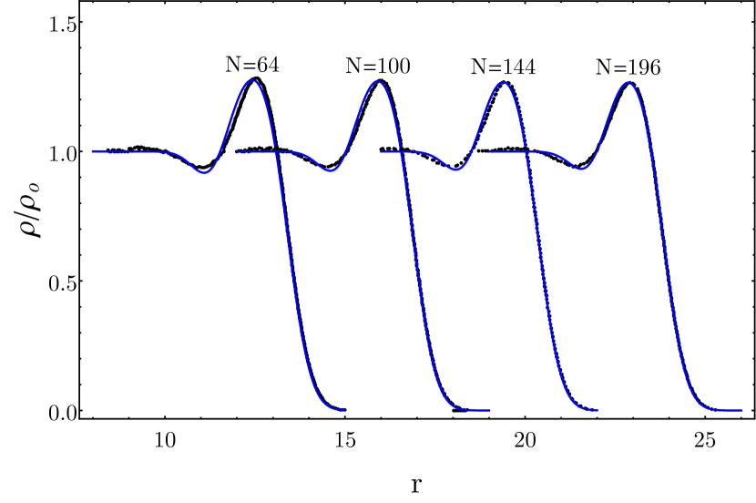
Figure 4: Numerical density profile of the $\nu=1/3$ Laughlin ground state for $N=64,100,144,196$ [35] (black points) and two-block fit (blue).

The overshoot is the result of highly non-trivial correlations inside the Laughlin state, but for what concern the density profile, it is possible to model it in terms of fermionic occupation numbers $n_{j}$ for momentum $j$, as follows:

$$\rho_{o}(r)=\langle\Omega|\rho(z,\bar{z})|\Omega\rangle_{\nu=1/3}=\sum_{j=0}^{\infty}|\phi_{j}(z,\bar{z})|^{2}\ n_{j}.$$ (4.1)

The $n_{j}$ correspond to the average over occupation numbers of very many Slater determinants contained in the Laughlin state.

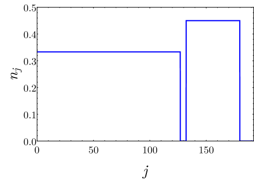
Figure 5: Occupation numbers $n_{j}$ of single particle states with momentum $j$ for fitting the $\nu=1/3$ Laughlin ground state density ($N=64$).

Let us discuss a simple two-block distribution of occupation numbers, as show in Fig.5. The first block is given by the flat droplet with $n_{j}=1/3$ but shortened by $\Delta j=-a$ from its natural extension $j_{\rm max}=3N-1$. The second block of variable height $n_{j}=h$ extends for $-b<\Delta j\leq-c$. These occupation numbers can actually be realized by a finite sum of Slater determinants. Two of the four parameters $\{a,b,c,h\}$ are fixed by the sum rules obeyed by the Laughlin state:

$$\int d^{2}r\ \rho_{o}=N,\qquad\int d^{2}r\;r^{2}\rho_{o}=\frac{mN(N-1)}{2}+N,\qquad\nu=\frac{1}{m}$$ (4.2)

while the two others are approximatively determined by the fit. The result are:

$$a\sim 8.00\sqrt{N},\qquad b\sim 7.35\sqrt{N},\qquad c\sim 1.40\sqrt{N},\qquad h\sim 0.45,$$ (4.3)

for $N=64,100,144,196$, with error of about $3$ on the last digit. Further analysis of the $N=200$ data of Ref.[36] confirms the values (4.3). The results of the fit are shown in Fig.4.

This analysis shows that the overshoot is characterized by angular momentum values $\Delta j\sim\sqrt{N}$. Since $R^{2}\sim mN$, its radial extension, $\Delta r\sim m\Delta j/(2R)$, approaches a constant for $R\to\infty$. Furthermore, the size $\Delta\rho$ of the modulation is also independent of the number of electrons (see Fig.4).

It is apparent that the edge excitations discussed in the previous Section are much smaller than the overshoot: they correspond to small deformations of the density outer slope and are manifestly unrelated to the non-trivial profile inside the droplet. Let us compare the respective sizes:

$$\begin{array}[]{l|l|l|l}&\Delta j&\Delta r&\Delta\rho\\ \hline\cr{\rm overshoot}&O(R)&>1&O(1)\\ {\rm edge\ excitation}&O(1)&O(1)&\leq\frac{1}{R}\\ \end{array}$$ (4.4)

The shape of the overshoot cannot be determined in our relativistic approach based on normal-ordered quantities, as already said. Nevertheless, its properties suggest us to extend the $W_{\infty}$ symmetry analysis to the regime of ‘large edge excitations’, possessing a finite $R\to\infty$ limit in terms of size, momenta and energies. In the following, we shall find that this generalization can be done and will give access to analytic results for bulk physics.

Let us add a side remark. The ground state density profile for other filling fractions $\nu=1/5,1/7,\dots$ presents more that one oscillation at the boundary and therefore the two-block fit must be replaced by a multi-block form. As explained in Ref.[36], these fluctuations near the boundary correspond to the preemptive freezing of Hall electrons into a Wigner crystal, starting from the outer parts of the droplet.

4.2 $W_{\infty}$ algebra in the bulk regime

4.2.1 The $R\to\infty$ limit for large excitations

We shall now extend our analysis to large edge excitations that possess a finite $R\to\infty$ limit. We reconsider the earlier derivation of the $W_{\infty}$ algebra for $\nu=1$ in Section 3.1, but perform another $R\to\infty$ limit, characterized by the following ranges of coordinates and angular momenta,

$$r=R+x,\quad x=O(1),\qquad m=R^{2}+m^{\prime},\quad m^{\prime}=O(R),\qquad{\bf k}=\frac{m^{\prime}}{R}=O(1),$$ (4.5)

where ${\bf k}$ is the momentum of waves propagating along the edge, approximately straight for $R\to\infty$.

Upon taking this limit in the expression of the Laplace transformed density (3.4), one finds the same expression up to an exponential prefactor (see the Appendix for the derivation),

$$\rho_{n}(\lambda)\quad\rightarrow\quad e^{-\frac{n^{2}}{8R^{2}}}\rho_{n}(\lambda),$$ (4.6)

and their algebra (3.10) is modified as follows:

$$\left[\rho_{k}(\lambda),\rho_{n}(\mu)\right]=A_{k,n}(\lambda,\mu)\;\rho_{k+n}(\eta)+\delta_{k+n,0}\;B_{k}(\eta),$$ (4.7)

where

$$A_{k,n}(\lambda,\mu)=e^{\frac{kn}{4R^{2}}}\left(x^{-\frac{n}{2}}y^{\frac{k}{2}}-x^{\frac{n}{2}}y^{-\frac{k}{2}}\right),$$

$$B_{k}(\eta)=e^{-\frac{k^{2}}{4R^{2}}}\sum_{i=1}^{k}z^{i-\frac{k+1}{2}},\qquad k>0,$$

$$t=\frac{1}{1+\lambda},\quad y=\frac{1}{1+\delta},\quad z=ty=\frac{1}{1+\eta}.$$ (4.8)

Note that the $W_{\infty}$ algebra is basically unchanged w.r.t. (3.10).

4.2.2 From Laplace to Fourier modes

Another useful observation about the $R\to\infty$ limit is that the radial coordinate $x=r-R$ actually become unbounded from below for density fluctuations that have finite support. Therefore, the Laplace transform on $r^{2}>0$ can be replaced by the Fourier transform in $x\in\mathbb{R}$. The relation between parameters are easily determined,

$$\lambda=-\frac{\partial}{\partial r^{2}}=-\frac{1}{2r}\frac{\partial}{\partial r}\sim-\frac{1}{2R}\frac{\partial}{\partial x}=-\frac{i{\bf p}}{2R},\qquad\quad R\to\infty,$$ (4.9)

where ${\bf p}=O(1)$ is the momentum conjugate to $x=O(1)$ and thus orthogonal to the boundary.

Laplace and Fourier transforms of the density are identified as follows:

$$\rho_{k}(\lambda)\ \rightarrow\ \rho_{k}({\bf p}),\qquad\quad\frac{1}{1+\lambda}\sim\exp\left(i\frac{{\bf p}}{2R}\right),$$ (4.10)

and the $W_{\infty}$ algebra becomes,

$$\left[\rho_{k}({\bf p}),\rho_{n}({\bf p^{\prime}})\right]=A_{k,n}({\bf p},{\bf p^{\prime}})\;\rho_{k+n}({\bf p+p^{\prime}})+\delta_{k+n,0}\;B_{k}({\bf p+p^{\prime}}),$$ (4.11)

where

$$A_{k,n}({\bf p},{\bf p^{\prime}})=e^{\frac{kn}{4R^{2}}}\left(e^{\frac{i}{4R}(k{\bf p^{\prime}}-n{\bf p})}-e^{\frac{-i}{4R}(k{\bf p^{\prime}}-n{\bf p})}\right),$$

$$B_{k}({\bf p+p^{\prime}})=e^{-\frac{k^{2}}{4R^{2}}}\sum_{\ell=1}^{k}e^{i\frac{\bf p+p^{\prime}}{2R}\left(\ell-\frac{k+1}{2}\right)},\qquad k>0.$$ (4.12)

Note that the $1/R$ dependence should be kept, because the indeces are $k,n=O(R)$: a finite $R\to\infty$ limit is achieved at the end of calculations.

The algebra (4.11) is similar to the Girvin-MacDonald-Platzman form (2.12), but there are two crucial differences:

• There is a central extension that originates from relativistic normal ordering and the norm of the Hilbert space for the edge theory.

• Ground state conditions as well as representations (values of Casimirs) are known. This permits analytic computation of observables as discussed in the following sections.

4.3 Bosonization of the short-range interaction

We now find the form of the Hamiltonian in the regime of large fluctuations. Consider the Gaussian two-body potential, parameterized by the variable $t>0$:

$$H_{t}=\frac{1}{2}\int d^{2}r_{1}d^{2}r_{2}\;\rho(\vec{r}_{1})\;\exp\left(-t|\vec{r}_{1}-\vec{r}_{2}|^{2}\right)\;\rho(\vec{r}_{2}).$$ (4.13)

This type of short-range potential yields relatively simple matrix elements for $R\to\infty$. Furthermore, by expanding in the $t\to\infty$ limit, one obtains the Haldane ultra-local potentials [1]. For example:

$$\delta^{(2)}(\vec{r}_{1}-\vec{r}_{2}) = \lim_{t\to\infty}\frac{t}{\pi}e^{-t|\vec{r}_{1}-\vec{r}_{2}|^{2}},$$ (4.14)

$$\nabla^{2}\delta^{(2)}(\vec{r}_{1}-\vec{r}_{2}) = \lim_{t\to\infty}\frac{-t^{2}}{\pi}\left(1+t\frac{\partial}{\partial t}\right)e^{-t|\vec{r}_{1}-\vec{r}_{2}|^{2}}.$$ (4.15)

The first interaction actually vanishes for fermionic systems, while the second one is the first Haldane potential for which the $\nu=1/3$ Laughlin state is the exact ground state.

The evaluation of the two-body matrix elements in the $\nu=1$ fermionic Fock space and their $R\to\infty$ limit (4.5) by saddle-point approximation is carried out in the Appendix, by extending results of Ref.[28]. After antisymmetrization with respect to fermion exchanges, the result is indeed found to behave as $O(1/t^{2})$ for large $t$, thus checking the vanishing of the delta interaction (4.14). This leading behavior determines the Haldane potential we are interested in. We obtain:

$$H=-\frac{2}{R}\sum_{r,s,k\in\mathbb{Z}}e^{-\frac{k^{2}}{4R^{2}}-\frac{(r-s+k)^{2}}{4R^{2}}}\left(\frac{k^{2}}{4R^{2}}-\frac{(r-s+k)^{2}}{4R^{2}}\right)c^{\dagger}_{s}c_{s-k}c^{\dagger}_{r}c_{r+k}.$$ (4.16)

In this expression, we omitted inessential numerical factors and used angular momentum indeces $\{r,s,k\}$ shifted to the edge, as in (4.5). The quadratic forms appearing in the matrix element are actually dictated by antisymmetrization.

The Hamiltonian can be bosonized using the following trick. Note that the first term in the exponential in (4.16) is the prefactor for $\rho_{k}(\lambda)$ in (4.6). The second term is actually the square of the coefficient in its Fock space expression (cf. (3.6) and (4.10)):

$$\rho_{k}({\bf p})=e^{-\frac{k^{2}}{8R^{2}}}\sum_{r}e^{i\frac{\bf p}{2R}\left(r+\frac{k-1}{2}\right)}c^{\dagger}_{r}c_{r+k}.$$ (4.17)

Using the Gaussian integral we can write,

$$H = -\frac{2}{R}\sum_{r,s,k\in\mathbb{Z}}\int_{-\infty}^{\infty}\frac{d{\bf q}}{2\sqrt{\pi}}e^{-\frac{{\bf q}^{2}}{4}}\left(\frac{k^{2}}{4R^{2}}+\left(\frac{\partial}{\partial{\bf q}}\right)^{2}\right)e^{i\frac{{\bf q}}{2R}\left(r+\frac{k}{2}-s+\frac{k}{2}\right)}e^{-\frac{k^{2}}{4R^{2}}}c^{\dagger}_{s}c_{s-k}c^{\dagger}_{r}c_{r+k}$$ (4.18)

$$= -\frac{1}{R}\sum_{k>0}\int_{-\infty}^{\infty}\frac{d{\bf q}}{2\sqrt{\pi}}\ e^{-\frac{{\bf q}^{2}}{4}}\left(\frac{k^{2}}{R^{2}}+{\bf q}^{2}-2\right)\rho_{-k}(-{\bf q})\rho_{k}({\bf q}).$$

In this expression, normal ordering with respect to the ground state (3.7) has been implemented, leading to $k\geq 0$. The $k=0$ term is singled out with factor one half [32]: however, this is non-vanishing on charged states (3.19) only, and should be removed for later evaluation of excitation spectra.

In conclusion, we have shown that the short-range interaction can be bosonized in the regime of large fluctuations. The resulting expression looks similar to the Fourier transform of the Haldane potential (4.15), in terms of momenta $\{{\bf q},{\bf k}=k/R\}$, orthogonal and longitudinal to the edge, respectively. Note the condition $k>0$ due to chirality.

Let us add some remarks:

• In the case of edge excitations, the momenta $\{r,s,k\}$ take finite values: approximating the exponential factor in (4.16) by one, we would get the Hamiltonian $H\sim\sum(k/R)^{2}\rho_{-k}\rho_{k}$ and recover the spectrum of capillary waves, $\varepsilon_{k}\sim-k^{3}/R^{3}$, as discussed in Ref. [28]. In the present case, we are interested in large fluctuations $k=O(R)$, thus the exponentials should be kept.

• The form of the Hamiltonian (4.18) can be modified by adding a one-body term: this can be done e.g. for enforcing translation invariance of the electron droplet, requiring a vanishing energy for ${\bf q}=0$ and $k=0,\pm 1$ [28]. However, this is not relevant for the following discussion of the $k=O(R)$ regime.

4.4 Spectrum of large neutral excitations: edge reconstruction

We reconsider the basic particle-hole edge excitation of Section 3.2, described by:

$$|\{{\bf n,p}\}\rangle=\rho_{-n}({\bf p})|\Omega\rangle,$$ (4.19)

where ${\bf n}=n/R>0$ is the momentum parallel to the edge in the extended range (4.5). We also allow a non-vanishing orthogonal momentum ${\bf p}$.

The energy of this excitation is given by the expectation value:

$$\varepsilon({\bf n,p})=\frac{\langle\{{\bf n,p}\}|H|\{{\bf n,p}\}\rangle}{\langle\{{\bf n,p}\}|\{{\bf n,p}\}\rangle}.$$ (4.20)

The expression to be evaluated at the numerator is,

$$-\frac{2}{R\sqrt{\pi}}\sum_{k>0}\int_{-\infty}^{\infty}d{\bf q}\;e^{-\frac{{\bf q}^{2}}{4}}\left(\frac{k^{2}}{4R^{2}}+\frac{\partial^{2}}{\partial^{2}{\bf q}}\right)\langle\Omega|\rho_{n}({\bf-p})\rho_{-k}({\bf-q})\rho_{k}({\bf q})\rho_{-n}({\bf p})|\Omega\rangle.$$ (4.21)

Using the ground state conditions (3.18),

$$\rho_{n}({\bf p})|\Omega\rangle=0,\qquad\quad n\geq 0,\quad\forall\;{\bf p},$$ (4.22)

the result is obtained by repeatedly using the commutators (4.11). Note that the bulk prefactor (3.5) for the density is not needed, since it cancels out in the expression (4.20). The result is (see the Appendix for details):

$$\!\!\!\!\!\varepsilon({\bf n,p}) = -\frac{2}{\bf n}\int_{0}^{\bf n}d{\bf k}\;e^{-\frac{{\bf k}^{2}}{4}}\left({\bf n-k}\right)\left[{\bf k}^{2}+\left({\bf n}^{2}-{\bf k}^{2}\right)\cos\left(\frac{\bf pk}{2}\right)e^{-\frac{{\bf n}^{2}}{4}}\right]$$ (4.23)

$$- \frac{e^{-\frac{{\bf n}^{2}}{4}}}{\bf n}\int_{0}^{\bf n}d{\bf k}\int_{0}^{\bf n}d{\bf k^{\prime}}e^{-\frac{({\bf k-k^{\prime}})^{2}}{4}}\left({\bf n}^{2}-({\bf k-k^{\prime}})^{2}\right)\cos\left(\frac{\bf p(k-k^{\prime})}{2}\right).$$

Note that this expression has a finite $R\to\infty$ limit once expressed in terms of momenta ${\bf n}$ and ${\bf p}$, as promised.

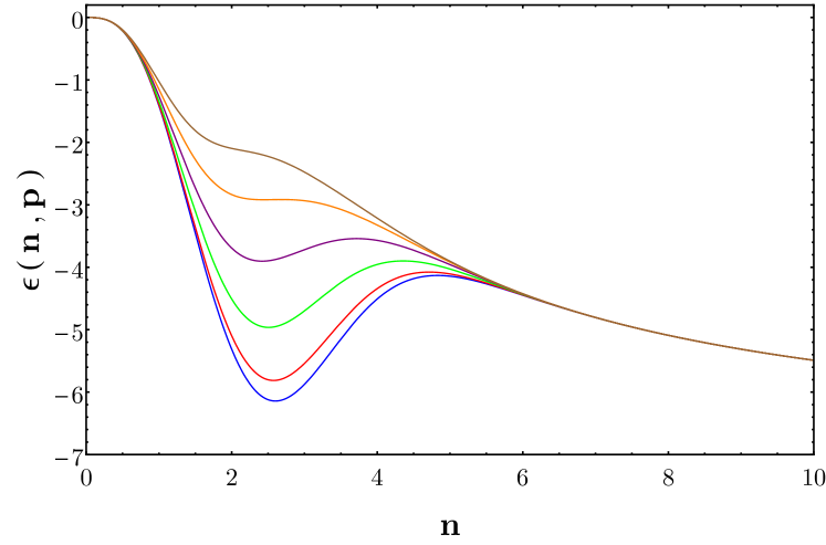
Figure 6: Energy spectrum $\varepsilon({\bf n,p})$ of $\nu=1$ large neutral excitations plotted as a function of ${\bf n}$ for values of ${\bf p}=0,1,\dots,5$ (from bottom to top).

The resulting energy spectrum is plotted in Fig.6 as a function of the momentum ${\bf n}$ for several values of ${\bf p}$. One can distinguish three behaviors:

• the edge regime for small ${\bf n}$, corresponding to the capillary waves, $\varepsilon({\bf n,p})\sim-{\bf n}^{3}$ [28].

• A local minimum for ${\bf k}={\bf k}_{o}\sim 2.6$ and ${\bf p}\lesssim 10$.

• A decreasing behavior asymptotically reaching a constant for large $\bf n$ (not seen in Figure).

Note that the Haldane potential is classically repulsive and this explains the decreasing and saturation of the spectrum at large k. There is however a fermionic exchange term that is attractive and causes the local minimum. This phenomenon is the so-called edge reconstruction, the tendency of the incompressible fluid droplet to split a thin ring to finite distance $x_{o}=O(\ell)$ [23]. Originally observed for Coulomb interaction, it is also present for short-range potentials. Upon adding a standard quadratic confining potential, corresponding to $\varepsilon({\bf n,p})\to\varepsilon({\bf n,p})+v{\bf n}$, one finds a minimum at finite ${\bf k}\lesssim 2.6$, called edge roton [24] (see Fig.7).

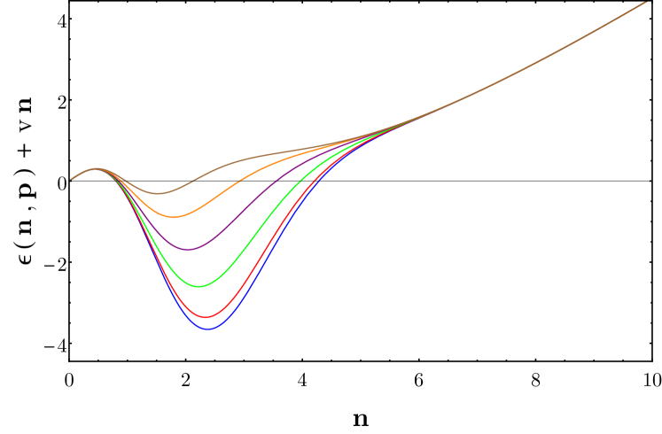
Figure 7: Energy spectrum $\varepsilon({\bf n,p})+v{\bf n}$ of $\nu=1$ large neutral excitations plotted as a function of ${\bf n}$ for values of ${\bf p}=0,1,\dots,5$ (from bottom to top).

In conclusion, we have found that the $W_{\infty}$ symmetry allows for analytic description of a non-trivial phenomena for quantum incompressible fluids in the range of large edge excitations, characterized by finite $R\to\infty$ limit.

Let us add some comments:

• The ansatz excitation (4.20) is actually Girvin-MacDonald-Platzman original one [26], but our geometry is different, being the half-plane; thus, the edge roton in Fig.7 is unrelated to the bulk magneto-roton (for $\nu<1$).

• The edge reconstruction phenomenon is qualitatively expected for any two-body interaction underlying the incompressible fluid state. For quantitative universal features, one should consider the density shape, to be discussed later.

• Fig.7 manifestly shows non-linear behaviors occurring beyond the conformal invariant regime. As already said, the validity of our results on this domain follows the $W_{\infty}$ algebra (4.11) and the ground state conditions (4.22), that also hold for $k\sim R\to\infty$. Thus, it is a consistent extension, supported by the results of Section 2.2.

• The expression (4.23) for $\varepsilon({\bf n,p})$ can be integrated in terms of error functions ${\rm erf}(x)$ without gaining in simplicity. This result was also obtained by using Laplace modes and the algebra (3.10); once rewritten in terms of momenta, as in (4.9), Eq. (4.23) is reproduced in the $R\to\infty$ limit (4.5).

4.4.1 Spectrum for fractional filling

The derivation of the spectrum (4.20) extends verbatim to $\nu=1/3$: the needed inputs, i.e. the bosonic form of the Hamiltonian (4.18), the algebra (4.11) and ground-state conditions (4.22) are unchanged, only the unit of length is redefined. From the analysis of Section 3.4, we know that the correct scaling is given by $r^{2}\to r^{2}/\sqrt{m}$ for filling $\nu=1/m$. This fact can be accounted for by replacing $\ell^{2}\to\ell^{2}\sqrt{m}$ in all quantities requiring a length scale. The expression of the spectrum (4.23), $\varepsilon({\bf n,p})\sim{\bf n}^{3}\ell^{2}$, acquires an overall factor $\sqrt{m}$ and the same factor multiplies all arguments of exponentials and cosinuses. Alternatively, one can leave the formula (4.23) unchanged but remembers to rescale $\ell^{2}$.

In table 1 we report our results for the edge roton minimum ${\bf k}_{o}$ and edge reconstruction distance $x_{o}$ (the latter is taken from density shape in Section 4.5), and compare them with the values found in the literature [23] [24]. Universality for these quantities is not to be expected, as said before.

4.4.2 Bulk momentum dependence

The energy spectrum found in the previous Section also depends on the momentum ${\bf p}$ orthogonal to the boundary, specifying the Fourier component for the radial modulation of excitations. It is found that $\varepsilon({\bf n,p})$ is even in ${\bf p}$, as expected; it is monotonically growing, eventually removing the minimum for ${\bf p}\gtrsim 10$ and asymptotically reaching a ${\bf p}$-independent curve for large values (see Fig,8). Actually, there is very little dependence on ${\bf p}$ outside the region of the minimum. The same qualitative behavior is found in the fractional case, only involving a rescaling of momenta.

The disappearance of the minimum can be interpreted as evidence that the radial modulation spoils the edge reconstruction effect, i.e. reduces the attractive exchange interaction.

The overall weak ${\bf p}$-dependence of the spectrum is a consequence of the compact support of the excitation created by $\rho_{-n}({\bf p})|\Omega\rangle$. Actually, this is localized on a region $|x|=O(1)$ and its Fourier transform is also localized around $|{\bf p}|=O(1)$. In conclusion, the ansatz excitation (4.19) analyzed in this Section is not really appropriate for creating a bulk density fluctuation.

$$\begin{array}[]{|l|l|l|l|l|}\hline\cr&{\bf k}_{o}(\nu=1)&x_{o}(\nu=1)&{\bf k}_{o}(\nu=1/3)&x_{o}(\nu=1/3)\\ \hline\cr W_{\infty}{\ \rm symmetry}&2.6&0.65&2.0&0.85\\ {\rm edge\ roton}&&&1.5&\\ {\rm edge\ reconstruction}&&\sim 2&&\\ \hline\cr\end{array}$$

Table 1: Minimum ${\bf k}_{o}$ of energy spectrum and positions $x_{o}$ obtained in our analysis versus results for edge reconstruction [23] and edge roton [24] (in units $\ell=1$).

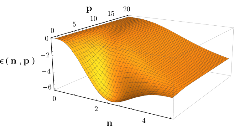
Figure 8: Energy spectrum $\varepsilon({\bf n,p})$ of large neutral excitations plotted as a function of ${\bf n}$ and ${\bf p}$ ($\nu=1$).

4.5 Spectrum of large charged excitations: bulk fluctuations

In the following, we find the energy spectrum for the excitation obtained by adding a big charge at the boundary, $Q={\bf t}R/m$, ${\bf t}=O(1)$. This is the ‘large’ version of the edge state described in Section 3.3, and is defined by:

$$|\{{\bf n,p;t}\}\rangle=\rho_{-n}({\mathbf{p}})|Q\rangle,\qquad\quad Q=\frac{{\bf t}R}{m},\qquad\nu=\frac{1}{m}.$$ (4.24)

We consider the expectation value,

$$\varepsilon({\bf n,p;t})=\frac{\langle\{{\bf n,p;t}\}|H|\{{\bf n,p;t}\}\rangle}{\langle\{{\bf n,p;t}\}|\{{\bf n,p;t}\}\rangle},$$ (4.25)

recalling that the Hamiltonian obeys $H|Q\rangle=0$ and is suitable for computing excitation energies. The derivation of the spectrum is obtained by using the $W_{\infty}$ algebra and the highest-weight state conditions, as in previous Sections. There are two additional terms w.r.t. the earlier calculation, owing to $\rho_{0}({\bf p})|Q\rangle\neq 0$, that are proportional to the expectation values of the density and its square.

These expectation values are given by the Casimir generating function (3.23) and (3.32): after replacing Laplace with Fourier variables according to (4.10), one obtains the form,

$$\frac{\langle Q|\rho_{0}({\bf p})|Q\rangle}{\langle Q|Q\rangle}=\frac{1}{m}\frac{e^{\frac{i{\bf pt}}{2}}-1}{i\frac{\bf p}{2R}},\qquad\qquad Q=\frac{{\bf t}R}{m},\qquad\nu=\frac{1}{m}$$ (4.26)

bearing on the discussion in Section 3.4. Note that this result can be simply obtained by Fourier transforming the (classical) droplet of hight $1/m$ and sharp boundary. As a matter of fact, this approximation is sufficient for the large excitation regime.

The energy spectrum (4.25) is found to be:

$$\varepsilon({\bf n,p;t})=\frac{\sqrt{m}\;e^{-\frac{{\bf n}^{2}\sqrt{m}}{4}}}{\bf n}\bigg{\{}$$

$$-2\int_{0}^{\bf n}d{\bf k}\;e^{-\frac{{\bf k}^{2}\sqrt{m}}{4}}\left({\bf n-k}\right)\left[{\bf k}^{2}e^{\frac{{\bf n}^{2}\sqrt{m}}{4}}+\left({\bf n}^{2}-{\bf k}^{2}\right)\cos\left(\frac{{\bf pk}\sqrt{m}}{2}\right)\right]$$

$$-\int_{0}^{\bf n}d{\bf k}\int_{0}^{\bf n}d{\bf k^{\prime}}e^{-\frac{({\bf k-k^{\prime}})^{2}\sqrt{m}}{4}}\left({\bf n}^{2}-({\bf k-k^{\prime}})^{2}\right)\cos\left(\frac{{\bf p(k-k^{\prime})}\sqrt{m}}{2}\right)$$

$$+2\frac{\sqrt{m}-1}{m}\int_{0}^{\bf n}d{\bf k}\int_{0}^{\frac{{\bf t}}{\sqrt{m}}}d{\bf k^{\prime}}\left[e^{-\frac{({\bf k-k^{\prime}})^{2}\sqrt{m}}{4}}\left({\bf n}^{2}-({\bf k-k^{\prime}})^{2}\right)\cos\left(\frac{{\bf p(k-k^{\prime})}\sqrt{m}}{2}\right)\right.$$

$$\qquad\qquad\qquad\qquad\qquad\qquad\quad-\ \left({\bf k^{\prime}}\to-{\bf k^{\prime}}\right)\bigg{]}\bigg{\}}.$$ (4.27)

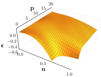
(a)

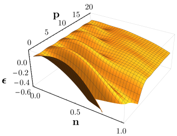
(b)

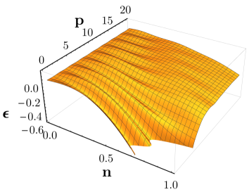
(c)

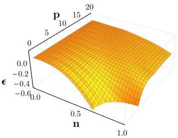
(d)

Figure 9: Energy spectrum $\varepsilon({\bf n,p;t})$ for large charged excitations plotted as a function of ${\bf n}$ and ${\bf p}$ for: (a) ${\bf t}=1$; (b) ${\bf t}=3$ (c) ${\bf t}=5$; (d) ${\bf t}=7$ ($\nu=1/3$).

The first two terms in this expression are the same as in the neutral $\nu=1$ case (4.23), suitably rescaled by $\ell^{2}\to\ell^{2}\sqrt{m}$, as explained before. The third term is the new charge-dependent part: it is of positive sign and non-vanishing for fractional fillings. Actually, adding a charge to the completely filled level does not change its shape, and only corresponds to a redefinition of value of $R$. Thus, it is not surprising that in this case the spectrum of excitations above neutral and charged ground states are equal.

In the fractional case, the ${\bf p}$ dependence of the spectrum is non-trivial: one sees dumped oscillations of period $T_{\bf p}\sim 15/{\bf t}$ for values of ${\bf n}$ not too big and charges ranging from ${\bf t}=1$ to ${\bf t}=7$ (see Fig. 9). This result shows that a finite deformation of the density at the boundary due to charge accumulation determines a response of the quantum incompressible fluid to bulk compressions. The properties of these excitations will be further discussed after computing the density profile in the next Section.

4.6 The density profile for large excitations

The shape of the fluctuations (4.24) is given by the expectation value,

$$\langle\rho_{0}({\bf s})\rangle=\frac{\langle\{{\bf n,p;t}\}|\rho_{0}({\bf s})|\{{\bf n,p;t}\}\rangle}{\langle\{{\bf n,p;t}\}|\{{\bf n,p;t}\}\rangle},\qquad\quad Q=\frac{{\bf t}R}{m},$$ (4.28)

where ${\bf s}$ is the momentum orthogonal to the boundary. This expression can be again evaluated by using the $W_{\infty}$ algebra in the Fourier basis (4.11). The definition of $\rho_{0}({\bf s})$ needs the bulk prefactor (3.5), that should be regularized in the map between Laplace and Fourier modes as follows:

$$(1+\lambda)^{-R^{2}}\rho_{0}(\lambda)\quad\to\quad|1+\lambda|^{-R^{2}}\rho_{0}({\bf p})\sim e^{-\frac{{\bf p}^{2}}{8}}\rho_{0}({\bf p}),\qquad\ \ \lambda\sim-\frac{i{\bf p}}{2R}.$$ (4.29)

The expression of $\langle\rho_{0}({\bf s})\rangle$ is Fourier transformed back to coordinate space in terms the variable $x=r-R$ near the edge, leading to the result (see Appendix):

$$\!\!\!\!\!\!\!\langle\delta\rho(x)\rangle = \frac{1}{\pi}\langle\rho_{0}(x)\rangle$$ (4.30)

$$= \frac{1}{m\pi}\bigg{\{}\frac{1}{2}\left({\rm erf}\left(\frac{{\bf t}-2x}{\sqrt{2}m^{\frac{1}{4}}}\right)+{\rm erf}\left(\frac{\sqrt{2}x}{m^{\frac{1}{4}}}\right)\right)$$

$$+ \frac{1}{\sqrt{2\pi}{\bf n}R}\int_{0}^{\bf n}d{\bf k}\left[\left(e^{-\frac{2}{\sqrt{m}}\left(x-\frac{t-{\bf k}\sqrt{m}}{2}\right)^{2}}-e^{-\frac{2}{\sqrt{m}}\left(x-\frac{t+{\bf k}\sqrt{m}}{2}\right)^{2}}\right)-({\bf t}=0)\right]$$

$$+ \frac{1}{\sqrt{2\pi}{\bf n}R}\int_{0}^{\bf n}d{\bf k}\left(e^{-\frac{2}{\sqrt{m}}\left(x-\frac{{\bf k}\sqrt{m}}{2}\right)^{2}}-e^{-\frac{2}{\sqrt{m}}\left(x-\frac{({\bf k-n})\sqrt{m}}{2}\right)^{2}}\right)\bigg{\}}.$$

We note that the first and second terms in this expression depend on the charge and vanish for ${\bf t}=0$. The first part reduces to the edge expression (3.34) for small fluctuations; the third part similarly matches the particle-hole excitation (3.35) (see Section 3.4). Note that all terms can be rewritten in terms of error functions, but the integral forms can be more compact.

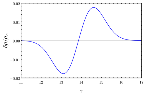
Figure 10: Density profile of ${\bf n}=1$ large particle-hole excitation for $\nu=1/3$. The overall factor $1/R$ is fixed to the value of $N=64$ electrons for comparison with the small excitation in Fig. 3.

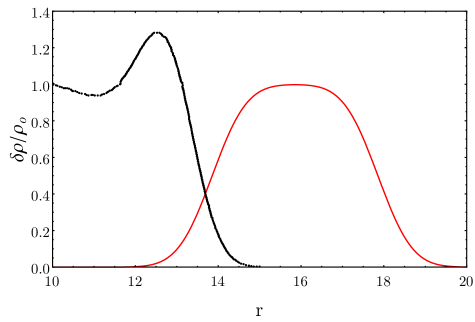
Figure 11: Density profile of the ground state (black dots) [35] and of the large charged excitation with ${\bf t}=8$ (red line) for $\nu=1/3$. Both profiles are independent of the number $N$ of electrons, up to a shift on the $r$ axis ($N=64$ here).

Let us first discuss the case ${\bf t}=0$, given by the third term in (4.30). Its profile looks like a regularized delta prime and is of size $O(1/R)$ (see Fig.10). Actually, this fluctuation is too small to describe the edge reconstruction, corresponding to a macroscopic displacement of matter, $\Delta\rho=O(1)$: this phenomenon is presumably given by the superposition of $O(R)=O(\sqrt{N})$ such particle-hole excitations, corresponding to the state $\prod_{i}^{R}\rho_{-n_{i}}({\bf s})|\Omega\rangle$. The computation of this energy is cumbersome, but at the semiclassical level it is approximately linear in its components, leading to an accumulation of the $\{n_{i}\}$ at the minimum of the spectrum (4.23) ${\bf n}_{o}\sim 2.6/m^{1/4}$. The density profile (4.30) has a maximum at $x_{o}\sim{\bf n}/4$ for large ${\bf n}$, but already accurate for ${\bf n}\sim{\bf n}_{o}$. This determines the splitting distance $x_{o}$ reported in Table 1.

In the case ${\bf t}\neq 0$, the first term in (4.30) is $\Delta\rho=O(1)$, while the two other pieces are $O(1/R)$ and can be neglected for $R\to\infty$. The shape of density deformation is a positive lump extending over several magnetic lengths. As shown in Fig. 11, the large charge accumulated at the edge is superposed to the ground state density terminating at $r\sim 15$ (for $N=64$ electrons). Let us incidentally note that this excitation cannot model the edge reconstruction effect because it is attached to the ground state density, not detached.

The large charged excitation has sufficient size and support to create a real bulk fluctuation: as a consequence, it energy spectrum shows a non-trivial dependence w.r.t. the bulk momentum ${\bf p}$, as seen in Fig. 9. At present, we do not have enough elements for associating the dumped fluctuations observed in the spectrum to specific bulk phenomena. The large charged fluctuation is still localized near the edge, and thus it is rather different from a low-energy density wave. In our analysis, we considered ansatz excitations that are extension of edge states: these are not the best suited for exploring bulk physics. We conclude that future investigations will require the formulation of better ansatz states within the analytic setup of this paper.

5 Conclusions

In this paper, we have shown that the $W_{\infty}$ symmetry of quantum Hall incompressible fluids can be used to describe the radial shape of edge excitations. We have identified two regimes of small and large fluctuations. The first domain includes the conformal invariant dynamics, whose energies and amplitudes vanish in the thermodynamic limit $R\to\infty$. While analytic and physical aspects were well understood in this case, we have provided the additional information of density profiles.

The second domain of large fluctuations was uncharted. We have seen that these excitations have a finite limit for $R\to\infty$ and partially extend into the bulk. We have considered some ansatz states and computed analytically their shape and energy spectrum for short-range Haldane potential: a minimum at finite momentum has been found that corresponds to the edge reconstruction phenomenon (and edge roton). Energy oscillations with respect to the bulk momentum have been observed in presence of a large charge accumulated at the boundary. Several results presented in this work can be checked by available numerical methods, as e.g. those of Ref.[36].

The $W_{\infty}$ symmetry approach has been formulated for $\nu=1$ and then extended to fractional fillings $\nu=1/m$ by bosonization. As a consequence, results in the integer and fractional cases are very similar, basically involving the (non-intuitive) magnetic-length scaling $\ell^{2}\to\ell^{2}\sqrt{m}$. This close correspondence is due to the composite fermion map that is built-in in our approach, as described in Section 2.

A consequence of this map is that the unperturbed Laughlin ground state cannot be compressed as much as the filled level: in technical terms, this property is expressed by the highest-weight conditions (4.22). Actually, we have seen that density fluctuations originates by decompressions in the region $\Delta r=O(1)$ at the boundary (see Section 4.4), and by adding boundary charge (Section 4.5). Our approach might not account for the compressibility of Laughlin plasma, as described e.g. by hydrodynamics [15]. However, it is believed that the composite-fermion theory captures the low-energy physics of Laughlin states; thus, our approach could be sufficient in this respect.

In introducing and motivating our work, we asked some questions about universality of bulk physics and the magneto-roton spectrum. We actually found a general framework for analytic studies of density fluctuations, providing some universal features. However, we could not identify the excitation corresponding to the magneto-roton. One open problem is that of finding appropriate ansatzes for density waves, since the states considered in Section 4 have finite support. We hope that further work will provide better approximate eigenstates in this range: for instance, one could study the spectrum according to the two-dimensional spin of excitations, since the leading low-energy branch is believed to have spin two [17] [18].

Another line of development is the study of $W_{\infty}$ symmetry for integer filling $\nu=n$ corresponding to several filled Landau levels. Such extension is possible because the symmetry act independently within each level [22]. In this formulation, one can describe the Jain states by bosonization, implementing the composite-fermion correspondence, and get insight into the multiple branches of bulk excitations known to appear in these cases [25].

Acknowledgments

A.C. would like to thank C. A. Trugenberger and G. R. Zemba for sharing their insight on the $W_{\infty}$ symmetry. We would like to thank P. Wiegmann for useful scientific exchanges. We also acknowledge the hospitality by the G. Galilei Institute for Theoretical Physics, Arcetri. This work is supported in part by the Italian Ministery of Education, University and Research under the grant PRIN 2017 “Low-dimensional quantum systems: theory, experiments and simulations.”

Appendix A Derivation of some formulas

In this Appendix, we give some details of the calculations done in the paper.

A.1 Small particle-hole excitation

The inverse Laplace transform of the expectation value (3.14) is:

$$\langle\delta\rho_{0}(r^{2})\rangle_{\{k\}}=-\int_{-i\infty}^{i\infty}\frac{d\lambda}{2\pi i}\,e^{\lambda r^{2}}\frac{\left(1-\left(1+\lambda\right)^{k}\right)^{2}}{k\lambda\left(1+\lambda\right)^{R^{2}+k+1}}.$$ (A.1)

The integral is done by closing the path on the semiplane Re$\left[\lambda\right]<0$ and calculating the residue at $\lambda=-1$ (recall that $R^{2}=N-1$ for $\nu=1$). This can be written as,

$$\langle\delta\rho_{0}(r^{2})\rangle_{\{k\}}=e^{-r^{2}}\frac{1}{\left(R^{2}+k\right)!}\left.\left(\frac{d}{dt}\right)^{R^{2}+k}\left(e^{tr^{2}}\frac{\left(1-t^{k}\right)^{2}}{k\left(1-t\right)}\right)\right|_{t=0},$$ (A.2)

where we defined $t=\lambda+1$. The following result is obtained:

$$\langle\delta\rho_{0}(r^{2})\rangle_{\{k\}}=\frac{e^{-r^{2}}}{k}\frac{r^{2R^{2}}}{\Gamma\left(R^{2}+1\right)}\left\{\left[\sum_{n=1}^{k}-\sum_{n=-k+1}^{0}\right]r^{2n}\frac{\Gamma\left(R^{2}+1\right)}{\Gamma\left(n+R^{2}+1\right)}\right\}.$$ (A.3)

In the edge limit (3.2) $r=R+x$ and $R\to\infty$, the Stirling approximations,

$$e^{-r^{2}}\frac{\left(r\right)^{2R^{2}}}{\Gamma\left(R^{2}+1\right)} \sim \frac{e^{-2x^{2}}}{\sqrt{2\pi}R}+O\left(\frac{1}{R^{2}}\right)\,,$$

$$\frac{\Gamma\left(R^{2}+a\right)}{\Gamma\left(R^{2}\right)} \sim R^{2a}\left(1+\frac{a\left(a-1\right)}{2R^{2}}+O\left(\frac{1}{R^{4}}\right)\right),\qquad a\sim O(1),$$ (A.4)

are used for obtaining the particle-hole edge excitation (3.15).

A.2 Small charged excitation

The inverse Laplace transform of the expectation value (3.23) is:

$$\langle\delta\rho_{0}(r^{2})\rangle_{Q}=\int_{-i\infty}^{i\infty}\frac{d\lambda}{2\pi i}\,e^{\lambda r^{2}}\frac{1-\left(1+\lambda\right)^{-Q}}{\lambda\left(1+\lambda\right)^{R^{2}+1}}.$$ (A.5)

We close again the path in the semiplane Re$[\lambda]<0$ and reduce to the evaluation of the residue at $\lambda=-1$. We get:

$$\langle\delta\rho_{0}(r^{2})\rangle_{Q}=e^{-r^{2}}\frac{r^{2R^{2}}}{\Gamma\left(R^{2}+1\right)}\sum_{n=1}^{Q}r^{2n}\frac{\Gamma\left(R^{2}+1\right)}{\Gamma\left(n+R^{2}+1\right)}.$$ (A.6)

Upon using the edge approximation (A.4), the expression (3.25) is found for small charged excitations.

A.3 Excitation of Laughlin states

We evaluate the inverse Laplace transform of the expectation value (3.32) for charged excitations of Laughlin state with $\nu=1/m$. The integrand in the following expression,

$$\langle\delta\rho_{0}(r^{2})\rangle_{Q}=\frac{e^{-\frac{r^{2}}{\sqrt{m}}}}{m}\int_{1-i\infty}^{1+i\infty}\frac{dt}{2\pi i}\,e^{\frac{tr^{2}}{\sqrt{m}}}\left(\frac{1-t^{-\frac{n}{\sqrt{m}}}}{\left(t-1\right)t^{\frac{R^{2}}{\sqrt{m}}}}\right),$$ (A.7)

has a branch cut starting from the pole $t=1+\sqrt{m}\lambda=0$ along the negative real axes, arg$(t)\in\left[-\pi,\pi\right]$. We consider the half ‘key-hole path’ of integration going around the singularity and the branch-cut. The integral is rewritten:

$$\langle\delta\rho_{0}(r^{2})\rangle_{Q}=\frac{e^{-\frac{r^{2}}{\sqrt{m}}}}{m}\left[\frac{\sin\left(\pi\left(\frac{R^{2}+n}{\sqrt{m}}\right)\right)}{\pi}\int_{0}^{\infty}dt\,\frac{e^{\frac{-tr^{2}}{\sqrt{m}}}}{\left(1+t\right)t^{\frac{R^{2}+n}{\sqrt{m}}}}-\left(n=0\right)\right].$$ (A.8)

The integral can be expressed in terms of the incomplete gamma function $\Gamma(a,z)$ and then analytically continued from negative to positive $a$ values, also using the Euler’s reflection formula for $\Gamma(a)$. The result is the expression (3.33) given in the text.

The following integral form the incomplete gamma function,

$$\Gamma(a,z)=\int_{z}^{\infty}e^{-t}t^{a-1},$$ (A.9)

is useful for computing the edge limit (3.2). We consider its derivative, expand it in $x=r-R$ for large $R$ and then integrate it back. The result (3.34) follows:

$$\langle\delta\rho_{0}(r^{2})\rangle_{Q}=\int_{-\infty}^{x}\partial_{y}\langle\delta\rho_{0}((R+y)^{2})\rangle_{Q}=\frac{e^{-\frac{2x^{2}}{\sqrt{m}}}}{m^{\frac{1}{4}}\sqrt{2\pi}R}\frac{n}{m}+O\left(\frac{1}{R^{2}}\right).$$ (A.10)

A.4 Large excitations $k=O(R)$

The Laplace transformed density (3.4) is now approximated within the ranges of coordinates and momenta given in (4.5). The Laplace modes for $k={\bf k}R$ become:

$$\rho_{k}(\lambda)=\sum_{j^{\prime}=-R^{2}}^{\infty}\frac{1}{(1+\lambda)^{R^{2}+{\bf k}R/2+j^{\prime}+1}}\frac{\Gamma\left(R^{2}+{\bf k}R/2+j^{\prime}+1\right)}{\left(\Gamma(R^{2}+j^{\prime}+1)\Gamma(R^{2}+{\bf k}R+j^{\prime}+1)\right)^{1/2}}c^{\dagger}_{j^{\prime}}c_{j^{\prime}+k}.$$ (A.11)

Upon using the improved asymptotic of the gamma function (cf. (A.4),

$$\frac{\Gamma\left(R^{2}+{\bf k}R+a\right)}{\Gamma\left(R^{2}\right)}\sim R^{2{\bf k}R+2a}e^{{\bf k}^{2}/2}\left(1+O\left(\frac{1}{R}\right)\right),$$ (A.12)

one finds:

$$\rho_{{\bf k}R}(\lambda)=e^{-{\bf k}^{2}/8}\frac{1}{\left(1+\lambda\right)^{R^{2}+\mu+1}}\sum_{j^{\prime}=-R^{2}}^{\infty}(1+\lambda)^{\mu-j^{\prime}-{\bf k}R/2}c_{j^{\prime}}^{\dagger}c_{j^{\prime}+{\bf k}R},\qquad R\to\infty.$$ (A.13)

Note the presence of the exponential prefactor $\exp{\left(-k^{2}/8R^{2}\right)}$, with $k={\bf k}R$, as introduced in (4.6).

A.5 Two-body Hamiltonian

Let us consider the matrix element (4.13) and expand the field operators (2.8) in Fock space. The expression to be evaluated is:

$$H_{t}=-\sum_{k,r,s\in\mathbb{Z}}M_{t}\left(k,r,s\right)c^{\dagger}_{s}c_{s-k}c^{\dagger}_{r}c_{r+k},$$ (A.14)

$$M_{t}\left(k,r,s\right)=-2\int_{0}^{\infty}dr_{1}\int_{0}^{\infty}dr_{2}r_{1}r_{2}\,I_{k}(2tr_{1}r_{2})e^{-\left(1+t\right)\left(r_{1}^{2}+r_{2}^{2}\right)}\frac{r_{1}^{2s+k}r_{2}^{2r-k}}{\sqrt{\left(s+k\right)!s!\left(r-k\right)!r!}},$$ (A.15)

where $I_{k}(z)$ is a Bessel function. The angular momentum indices $\{r,s,k\}$ and the radial coordinates are shifted and expanded in large excitation limit (4.5). The suitable asymptotic of the Bessel function is the following:

$$I_{k}\left(z\right)\sim\frac{e^{z-\frac{k^{2}}{2z}}}{\sqrt{2\pi z}}\left(1+O\left(\frac{1}{z}\right)+O\left(\frac{k^{4}}{z^{3}}\right)\right),\qquad z\to\infty,\quad k=O(\sqrt{z}).$$ (A.16)

The $r_{1},r_{2}$ integrals in (A.15) are computed by saddle point method following the same steps as in Ref.[28], but the results are now valid in the range of large excitations. We find the result:

$$H_{t}=\frac{2}{Rt^{2}}e^{-\frac{k^{2}+\left(r-s+k\right)^{2}}{4R^{2}}}\left(k^{2}-\left(r-s-k\right)^{2}\right)+O\left(\frac{1}{t^{3}}\right),$$ (A.17)

where we also antisymmetrized $M_{t}\left(r,s,k\right)$ respect to the fermion exchange $\{r\to s,\,s\to r,\,k\to-k\}$. Finally, taking the $t\to\infty$ limit (4.15) for (A.17), the result (4.16) for Haldane potential is obtained.

A.6 Energy spectrum of large excitations

The expectation value of the Hamiltonian (4.25) involves the expression:

$$\langle Q|\rho_{n}({\bf-p})\rho_{-k}({\bf-q})\rho_{k}({\bf q})\rho_{-n}({\bf p})|Q\rangle,\qquad\quad k>0,$$ (A.18)

that can be rewritten as,

$$\langle Q|\left[\rho_{n}({\bf-p}),\rho_{-k}({\bf-q})\right]\left[\rho_{k}({\bf q}),\rho_{-n}({\bf p})\right]Q\rangle.$$ (A.19)

The evaluation of the commutators with the help of the algebra (4.11) gives three terms:

$$A_{n,-k}(-{\bf p},-{\bf q})A_{k,-n}({\bf p},{\bf q})\langle Q|\rho_{n-k}({\bf-p-q})\rho_{k-n}({\bf p+q})|Q\rangle$$

$$+\delta_{n,k}A_{n,-n}(-{\bf p},-{\bf q})B_{n}({\bf p+q})\langle Q|\rho_{0}({\bf p+q})|Q\rangle+h.c.$$

$$+\delta_{n,k}B_{n}({\bf-p-q})B_{n}({\bf p+q})\langle Q|Q\rangle.$$ (A.20)

For vanishing charge $Q=0$, i.e. for neutral excitations analyzed in Section 4.4, the term in the second line of (A.20) vanishes, while the first part can be replaced by the commutator $\left[\rho_{n-k}({\bf-p-q}),\rho_{k-n}({\bf p+q})\right]$, for $k<n$. In the charged case, the non-vanishing second term is proportional to $\langle\rho_{0}\rangle$, while the expression in the first line acquires the $k=n$ contribution proportional to $\langle|\rho_{0}|^{2}\rangle$. Thus, there are two terms for $Q=0$ and four for $Q\neq 0$.

All contributions are summed over $k>0$ in the Hamiltonian and contain other summations in the $B_{n}$ terms. Discrete summations can be approximated by integrals for large excitations $n={\bf n}R$:

$$\frac{1}{R}\sum_{k=1}^{{\bf n}R}=\int_{0}^{{\bf n}}d{\bf k},\qquad k={\bf k}R.$$ (A.21)

Note that in this limit the large contributions from the density expectation value (4.26) $\langle\rho_{0}\rangle=O(R)$ can never be neglected. With these ingredients, the energies of neutral and charged large excitations, respectively (4.23) and (4.27), are obtained.

The corresponding expressions in the fractional case $\nu=1/m$ are obtained by scaling $\ell^{2}\to\ell^{2}\sqrt{m}$ in all dimensionful quantities, keeping in mind that the dimensionless $\langle\rho_{0}\rangle$ acquires an extra factor $1/\sqrt{m}$ from (3.31).

A.7 Large density profiles

The expectation value (4.28) can be written as:

$$\langle\rho_{0}({\bf s})\rangle=\frac{\langle Q|\left[\rho_{n}({\bf-p}),\rho_{0}({\bf s})\rho_{-n}({\bf p})\right]|Q\rangle}{\langle Q|\left[\rho_{n}({\bf-p}),\rho_{-n}({\bf p})\right]|Q\rangle},$$ (A.22)

being $n>0$. The use of the algebra (4.11) leads to three terms:

$$\!\!\!\!\!\langle\rho_{0}({\bf s})\rangle = \frac{\langle Q|\rho_{0}({\bf s})|Q\rangle}{\langle Q|Q\rangle}$$ (A.23)

$$+ \frac{A_{n,0}({\bf-p},{\bf s})A_{n,-n}({\bf-p+s,p})}{B_{n}(0)}\frac{\langle Q|\rho_{0}({\bf s})|Q\rangle}{\langle Q|Q\rangle}$$

$$+ \frac{A_{n,0}({\bf-p},{\bf s})B_{n}({\bf s})}{B_{n}(0)}.$$

For large charge $Q=tR/m$ and angular momentum $n={\bf n}R$, the first term is of order $O(1)$ while the two others are $O(1/R)$. The inverse Fourier transform of $\langle\rho_{0}({\bf s})\rangle$ can be formulated directly w.r.t. the boundary variable $x=r-R$, after including the bulk prefactor (4.29), as follows:

$$\langle\rho_{0}(x)\rangle=\frac{1}{4\pi R}\int dx\;e^{-i{\bf s}x-{\bf s}^{2}/8}\langle\rho_{0}({\bf s})\rangle.$$ (A.24)

The result (4.30) is obtained.

References

- [1] R. E. Prange, S. M. Girvin, The Quantum Hall Effect, Springer, Berlin (1987).
- [2] R. B. Laughlin, Quantized Hall conductivity in two-dimensions, Phys. Rev. Lett. B 23 5632(R).
- [3] X. G. Wen, Quantum Field Theory of Many-body Systems, Oxford Univ. Press, Oxford (2007).
- [4] G. Moore, N. Read, Nonabelions in the fractional quantum hall effect, Nucl. Phys. B 360 (1991) 362.
- [5] A. Cappelli, G. Viola, Partition Functions of Non-Abelian Quantum Hall States, J. Phys. A 44 (2011) 075401.
- [6] X. G. Wen, A. Zee, Shift and spin vector: New topological quantum numbers for the Hall fluids, Phys. Rev. Lett. 69 (1992) 953 [Phys. Rev. Lett. 69 (1992) 3000]; J. Fröhlich, U. M. Studer, Gauge invariance and current algebra in nonrelativistic many body theory, Rev. Mod. Phys. 65 (1993) 733.
- [7] J. K. Jain, Thirty Years of Composite Fermions and Beyond, arXiv:2011.13488.
- [8] D. T. Son, Is the Composite Fermion a Dirac Particle?, Phys. Rev. X 5 (2015) 031027.
- [9] B. I. Halperin, P. A. Lee, N. Read, Theory of the half filled Landau level, Phys. Rev. B 47 (1993) 7312.
- [10] E. H. Fradkin, Field Theories of Condensed Matter Physics, II edition, Cambridge Univ. Press, Cambridge (2013).
- [11] R. Shankar, Theories of the Fractional Quantum Hall Effect, arXiv:cond-mat/0108271, C. Berthier, L.P. Lévy, G. Martinez Eds., High Magnetic Fields, Lecture Notes in Physics, vol. 595, Springer, Berlin (2002).
- [12] V. Pasquier, F. D. M. Haldane, A dipole interpretation of the state, Nucl. Phys. B 516 (1998) 719.
- [13] N. Read, Lowest-Landau-level theory of the quantum Hall effect: The Fermi-liquid-like state of bosons at filling factor one, Phys. Rev. B 58 (1998) 16262.
- [14] J. K. Jain, R. K. Kamilla, Composite fermions in the Hilbert space of the lowest electronic Landau level, Int. J. Mod. Phys. B 11 (1997) 2621.
- [15] P. B. Wiegmann, Quantum Hydrodynamics, Rotating Superfluid and Gravitational Anomaly, J. Exp. Theor. Phys. 129 (2019) 642; Inner Nonlinear Waves and Inelastic Light Scattering of Fractional Quantum Hall States as Evidence of the Gravitational Anomaly, Phys. Rev. Lett. 120 (2018) 086601.
- [16] F. D. M. Haldane, "Hall viscosity" and intrinsic metric of incompressible fractional Hall fluids, arXiv:0906.1854; Geometrical Description of the Fractional Quantum Hall Effect, Phys. Rev. Lett. 107 (2011) 116801; Self-duality and long-wavelength behavior of the Landau-level guiding-center structure function, and the shear modulus of fractional quantum Hall fluids, arXiv:1112.0990. Y. Park, F. D. M. Haldane, Guiding-center Hall viscosity and intrinsic dipole moment along edges of incompressible fractional quantum Hall fluids, Phys. Rev. B 90 (2014) 045123.
- [17] A. Gromov, D. T. Son, “Bimetric Theory of Fractional Quantum Hall States, Phys. Rev. X 7 (2017) 041032.
- [18] S. Golkar, D. X. Nguyen, M. M. Roberts, D. T. Son, Higher-Spin Theory of the Magnetorotons, Phys. Rev. Lett. 117 (2016) 216403.
- [19] A. Cappelli, C. A. Trugenberger and G. R. Zemba, Infinite symmetry in the quantum Hall effect, Nucl. Phys. B 396 (1993) 465; Large N Limit in the Quantum Hall Effect, Phys. Lett. B 306 (1993) 100.
- [20] S. Iso, D. Karabali and B. Sakita, Fermions in the lowest Landau level: Bosonization, W infinity algebra, droplets, chiral bosons, Phys. Lett. B 296 (1992) 143; One-dimensional fermions as two-dimensional droplets via Chern-Simons theory, Nucl. Phys. B 388 (1992) 700.
- [21] A. Cappelli, C. A. Trugenberger and G. R. Zemba, Classification of quantum Hall universality classes by W(1+infinity) symmetry, Phys. Rev. Lett. 72 (1994) 1902.
- [22] A. Cappelli and L. Maffi, Bulk-Boundary Correspondence in the Quantum Hall Effect, J. Phys. A 51 (2018) 365401.
- [23] C. de C. Chamon and X. G. Wen, Sharp and smooth boundaries of quantum Hall liquids, Phys. Rev. B 49 (1994) 8227; X. Wan, K. Yang, E. H. Rezayi, Reconstruction of Fractional Quantum Hall Edges, Phys. Rev. Lett. 88 (2002) 056802.
- [24] S. Jolad, D. Sen, J. K. Jain, Fractional quantum Hall edge: Effect of nonlinear dispersion and edge roton, Phys. Rev. B 82 (2010) 075315.
- [25] V. W. Scarola, K. Park, J. K. Jain, Rotons of composite fermions: Comparison between theory and experiment, Phys. Rev. B 61 (2000) 13064; I. V. Kukushkin, J. H. Smet, V. W. Scarola, V. Umansky, K. von Klitzing, Dispersion of the Excitations of Fractional Quantum Hall States, Science 324 (2009) 1044.
- [26] S. M. Girvin, A. H. MacDonald and P. M. Platzman, Magneto-roton theory of collective excitations in the fractional quantum Hall effect, Phys. Rev. B 33 (1986) 2481.
- [27] A. Cappelli, C. A. Trugenberger and G. R. Zemba, Stable hierarchical quantum hall fluids as W(1+infinity) minimal models, Nucl. Phys. B 448 (1995) 470; W(1+infinity) minimal models and the hierarchy of the quantum Hall effect, Nucl. Phys. Proc. Suppl. 45A (1996) 112 [Lect. Notes Phys. 469 (1996) 249];
- [28] A. Cappelli, C. A. Trugenberger and G. R. Zemba, W(1+infinity) dynamics of edge excitations in the quantum Hall effect, Annals Phys. 246 (1996) 86.
- [29] P. Di Francesco, P. Mathieu, D. Sénéchal, Conformal Field Theory, Springer-Verlag, New York (1997).
- [30] M. Flohr, R. Varnhagen, Infinite symmetry in the fractional quantum Hall effect, J. Phys. A 27 (1994) 3999.
- [31] V. Kac, A. Radul, Quasifinite highest weight modules over the Lie algebra of differential operators on the circle, Comm. Math. Phys. 157 (1993) 429; H. Awata, M. Fukuma, Y. Matsuo, S. Odake, Representation theory of the Algebra, Prog. Theor. Phys. Suppl. 118 (1995) 343; E. Frenkel, V. Kac, A. Radul and W. Wang, and with central charge , Comm. Math. Phys. 170 (1995) 337.
- [32] A. Cappelli, G. V. Dunne, C. A. Trugenberger and G. R. Zemba, Conformal symmetry and universal properties of quantum Hall states, Nucl. Phys. B 398 (1993) 531.
- [33] A. Cappelli, L. S. Georgiev, I. T. Todorov, Parafermion Hall states from coset projections of Abelian conformal theories, Nucl. Phys. B 599 (2001) 499.
- [34] H. Azuma, W(infinity) algebra in the integer quantum Hall effects, Prog. Theor. Phys. 92 (1994) 293.
- [35] O. Ciftja, C. Wexler, Monte Carlo simulation method for Laughlin-like states in a disk geometry, Phys. Rev. B 67 (2003) 075304; N. Datta, R. Morf, R. Ferrari, Edge of the Laughlin droplet, Phys. Rev. B 53 (1996) 10906.
- [36] G. Cardoso, J.-M. Stéphan, A. G. Abanov, The boundary density profile of a Coulomb droplet. Freezing at the edge, arXiv:2009.02359.
- [37] T. Can, P. J. Forrester, G. Téllez and P. Wiegmann Singular behavior at the edge of Laughlin states Phys. Rev. B 89 (2014) 235137.