The short-term rational Lanczos method and applications

Abstract

Rational Krylov subspaces have become a reference tool in dimension reduction procedures for several application problems. When data matrices are symmetric, a short-term recurrence can be used to generate an associated orthonormal basis. In the past this procedure was abandoned because it requires twice the number of linear system solves per iteration compared with the classical long-term method. We propose an implementation that allows one to obtain the rational subspace reduced matrices at lower overall computational costs than proposed in the literature by also conveniently combining the two system solves. Several applications are discussed where the short-term recurrence feature can be exploited to avoid storing the whole orthonormal basis. We illustrate the advantages of the proposed procedure with several examples.

1 Introduction

Given a symmetric matrix $A\in{\mathbb{R}}^{n\times n}$ and a unit norm vector $v\in{\mathbb{R}}^{n}$, we are interested in analyzing the algebraic recurrence that generates the rational Krylov subspace

(1) $${\cal K}_{m}(A,v,\bm{\xi}_{m})={\rm span}\left\{v,(I-\xi_{1}^{-1}A)^{-1}v,\ldots,\prod_{j=1}^{m-1}(I-\xi_{j}^{-1}A)^{-1}v\right\},$$

and in the applicability of the computed quantities; here $\bm{\xi}_{m}=[\xi_{1},\ldots,\xi_{m-1}]$ with $\xi_{i}\neq 0$ are such that $I-\xi_{i}^{-1}A$ is nonsingular for $i=1,\ldots,m-1$. In the considered applications $A$ is definite (either positive or negative), for which strong theoretical arguments for the selection of the $\xi_{i}$ have been discussed, see [23, 34] and references therein. In our context, the corresponding theoretical setting suggests that the eigenvalues of $A$ and $\xi_{i}$ have opposite sign, an hypothesis that we will assume throughout. By relying on efficient sparse solvers for linear systems, rational Krylov subspaces have become a major tool in a variety of application problems, including eigenvalue approximation, dynamical system reduction, matrix equation solution, and matrix function and bilinear form evaluations [32, 6, 22, 21, 28, 33, 51]. An orthonormal basis $\{q_{1},\ldots,q_{m}\}$ for ${\cal K}_{m}(A,v,\bm{\xi}_{m})$ can be determined by using the Gram-Schmidt procedure as $q_{1}=v$ and

$$\hat{q}_{j+1}:=\left(I-\xi_{j}^{-1}A\right)^{-1}q_{j},\qquad h_{j+1,j}q_{j+1}=\hat{q}_{j+1}-Q_{j}h_{j},$$

where $h_{j}=Q_{j}^{T}\hat{q}_{j+1}$, $Q_{j}=[q_{1},\ldots,q_{j}]$ and $h_{j+1,j}$ is the normalization factor for $q_{j+1}$ for $j=1,\ldots,m$ [51, Eq. (4.15)]. This can be viewed as a rational variant of the Arnoldi iteration. The parameters (or shifts) $\bm{\xi}_{m}=[\xi_{1},\ldots,\xi_{m-1}]$ can be computed a-priori or determined adaptively as the space grows. The vector $h_{j}$ contains the orthogonalization coefficients, so that $Q_{j}$ has orthonormal columns for $j=1,\ldots,m$.

For $A$ symmetric, in [18] a short-term recurrence was introduced to generate an orthonormal basis of rational functions associated with ${\cal K}_{m}(A,v,\bm{\xi}_{m})$, from which a short-term recurrence can be derived for the basis $\{q_{1},\ldots,q_{m}\}$ [33].

The short-term recurrence yielding an orthonormal basis of the polynomial Krylov subspace generated by a symmetric $A$ was introduced by Lanczos [40], and it is thus referred to as the Lanczos iteration. This recurrence allows one to store few $n$-dimensional vectors, leading to major savings in various approximation problems where the whole basis is otherwise not needed. Thanks to the work in [18, 33], similar advantages can be envisioned in the rational case. Güttel in [33, p. 46] says: “Note that in each iteration of Algorithm 2 two linear systems with $I-A/\xi_{j}$ need to be solved […]. Hence, this algorithm is in general not competitive with the rational Arnoldi algorithm if the poles $\xi_{j}$ vary often. Moreover, we will make explicit use of the orthogonality of the rational Krylov basis $V_{m+1}$ when computing Rayleigh–Ritz approximations for $f(A)b$ (see Chapter 6). In this case full orthogonalization of $V_{m+1}$ is required anyway and one cannot take advantage of the short recurrence”. In spite of the elegant derivation, these considerations led Güttel to discard the short-term iteration in his application setting.

We claim that in spite of the extra cost per iteration, the rational short-term recurrence does provide an appealing framework for a variety of approximation problems. Our contribution is two-fold. First, we propose a new implementation of the short-term recurrence that: i) alleviates the computational costs associated with the two solves by combining them into a single linear system solve with multiple right-hand sides; ii) derives the entries of the reduced matrix $J_{m}:=Q_{m}^{T}AQ_{m}$ as the iterations proceed, without using $Q_{m}$ or explicitly solving $m\times m$ linear systems. Second, we illustrate the advantages of the obtained implementation in the numerical treatment of several application problems that do not require the whole basis matrix $Q_{m}=[q_{1},\ldots,q_{m}]$; these include the approximation of quadratic and bilinear forms in general, and quantities of interest in control, such as the estimation of the $\mathcal{H}_{2}$-norm of (parametric) linear time-invariant systems and of the optimal feedback control function. We will refer to this implementation as the $Q_{m}$-less computation.

We also start a discussion on the behavior of the obtained recurrence in finite precision arithmetic. Our matrix relations and experimental evidence seem to suggest that the short-term iteration is affected by round-off error accumulations similar to those of the classical Lanczos method. A deeper analysis of this crucial aspect deserves a dedicated research, it will thus be postponed to future work.

The synopsis of the paper is as follows. In section 2 we revisit the rational Lanczos iteration. An efficient, basis-free procedure to compute the matrix $J_{m}=Q_{m}^{T}AQ_{m}$ is derived in section 2.1, while in section 2.2 the novel implementation of the rational Lanczos method is illustrated. A panel of applications where the rational Lanczos method can be successfully employed is presented in section 3. These include numerical approximations of quadratic and bilinear forms (section 3.1), matrix function trace estimation (section 3.2), $\mathcal{H}_{2}$-norm computation for LTI systems (section 3.3), and LQR feedback control approximations (section 3.4). In section 4 some preliminary remarks on the behavior of the rational Lanczos method in finite precision arithmetic are reported. Our conclusions are given in section 5, while in the appendix the block rational Lanczos algorithm is given.

2 The short-term rational Krylov iteration

Based on the thorough analysis of orthogonal rational functions in [13], the authors of [18, Th. 4.2] developed a three-term recurrence relation to generate a sequence of orthogonal rational functions associated with the rational Krylov subspace (1); see also [18]. This elegant construction was further developed in [33, Section 5.2], leading to the following vector recurrence for $j\geq 1$,

(2) $$\beta_{j}\left(I-\xi_{j}^{-1}A\right)q_{j+1}=Aq_{j}-\alpha_{j}\left(I-\xi_{j-1}^{-1}A\right)q_{j}-\beta_{j-1}\left(I-\xi_{j-2}^{-1}A\right)q_{j-1},$$

where, with the usual convention that $1/\infty=0$, $\xi_{-1}:=\infty$, $\xi_{0}:=\infty$, $\beta_{0}=0$, $q_{0}=0$, and $q_{1}=v/\|v\|$. By setting

$$r:=(I-\xi_{j}^{-1}A)^{-1}(Aq_{j}+\beta_{j-1}\xi_{j-2}^{-1}Aq_{j-1})-\beta_{j-1}q_{j-1},\,\quad s:=(I-\xi_{j}^{-1}A)^{-1}(I-\xi_{j-1}^{-1}A)q_{j},$$

the coefficients $\alpha_{j}$ and $\beta_{j}$ are computed as $\alpha_{j}=(r^{T}q_{j})/(s^{T}q_{j})$, and $\beta_{j}=\|r-\alpha_{j}s\|$. A simple rearrangement of the terms leads to the following more compact notation,

$$A[q_{j-1},q_{j},q_{j+1}]\begin{bmatrix}\frac{\beta_{j-1}}{\xi_{j-2}}\\ \frac{\alpha_{j}}{\xi_{j-1}}+1\\ \frac{\beta_{j}}{\xi_{j}}\end{bmatrix}=[q_{j-1},q_{j},q_{j+1}]\begin{bmatrix}\beta_{j-1}\\ \alpha_{j}\\ \beta_{j}\end{bmatrix},$$

which, after $m$ iterations gives the Arnoldi-like relation

(3) $$AQ_{m+1}\underline{K}_{m}=Q_{m+1}\underline{H}_{m},\quad{\rm with}\quad\underline{K}_{m}=\underline{I}_{m}+D_{m}^{-1}\underline{H}_{m}\in{\mathbb{R}}^{(m+1)\times m},$$

where $\underline{I}_{m}$ is the $(m+1)\times m$ identity matrix and $D_{m}={\rm diag}(\xi_{0},\ldots,\xi_{m})$. Hence

$$\underline{K}_{m}=\begin{bmatrix}1&0&&\vspace{3pt}\\ \frac{\beta_{1}}{\xi_{1}}&1+\frac{\alpha_{2}}{\xi_{1}}&\frac{\beta_{2}}{\xi_{1}}\\ &\frac{\beta_{2}}{\xi_{2}}&1+\frac{\alpha_{3}}{\xi_{2}}&\hskip 2.0pt\ddots&\\ &&\ddots&\ddots&\frac{\beta_{m-1}}{\xi_{m-2}}\vspace{4pt}\\ &&&\frac{\beta_{m-1}}{\xi_{m-1}}&1+\frac{\alpha_{m}}{\xi_{m-1}}\vspace{4pt}\\ &&&&\frac{\beta_{m}}{\xi_{m}}\vspace{4pt}\end{bmatrix},\quad\underline{H}_{m}=\begin{bmatrix}\alpha_{1}\vspace{3pt}&\beta_{1}&&\\ \beta_{1}&\alpha_{2}&\beta_{2}&\\ &\beta_{2}&\alpha_{3}&\ddots\\ &&\ddots&\ddots&\beta_{m-1}\vspace{4pt}\\ &&&\beta_{m-1}&\alpha_{m}\vspace{4pt}\\ &&&&\beta_{m}\vspace{4pt}\end{bmatrix}.$$

The relation in (3) can also be written as

(4) $$AQ_{m}K_{m}=Q_{m}H_{m}+\beta_{m}\left(I-\xi_{m}^{-1}A\right)q_{m+1}e_{m}^{T},$$

with $K_{m}$ and $H_{m}$ the leading $m\times m$ upper parts of $\underline{K}_{m}$ and $\underline{H}_{m}$, respectively. Here and in the following, $e_{j}$ denotes the $j$th column of the identity matrix, whose dimension is clear from the context. Hence, we resume the standard form for the rational Krylov iteration [51]. This means that in exact arithmetic the rational Lanczos and rational Arnoldi recurrences compute the same basis, provided the same set of shifts is employed in the basis construction.

Thanks to the irreducibility of $\underline{H}_{m}$, it follows from (4) that if the matrix $K_{m}$ is singular, then $[Q_{m},(I-\xi_{m}^{-1}A)q_{m+1}]$ is not full rank, which occurs if and only if the subspace $\mathcal{K}_{m}(A,v,\bm{\xi}_{m})$ is $A$-invariant, i.e., $A\mathcal{K}_{m}(A,v,\bm{\xi}_{m})=\mathcal{K}_{m}(A,v,\bm{\xi}_{m})$. In the $A$-invariant case we have a lucky termination of the algorithm. Hereafter we thus always assume $K_{m}$ to be invertible. Like for the standard Lanczos procedure, the matrix $J_{m}=Q_{m}^{T}AQ_{m}$ represents the projection and restriction of $A$ onto the range space of $Q_{m}$. However, while in the (standard) Arnoldi process this matrix is tridiagonal, the matrix $J_{m}$ is generally full. A detailed analysis of the structure and decay properties of the entries of $J_{m}$ can be found in [49]; see also [50]. The matrix $J_{m}$ appears in projection methods for solving problems such as linear and quadratic matrix equations and matrix functions evaluations. Classical implementations of the rational Lanczos recurrence rely on the whole matrix $Q_{m}$. In the following we show that this can be avoided, leading to memory savings in a variety of application problems.

2.1 On the computation of $J_{j}=Q_{j}^{T}AQ_{j}$

In this section we derive a recurrence for computing the small dimensional matrix $J_{j}=Q_{j}^{T}AQ_{j}$ without using $Q_{j}$ or explicitly solving small size linear systems with $K_{j}$ at each iteration $j$.

Setting $J_{j+1}=Q_{j+1}^{T}AQ_{j+1}$ and multiplying (4) by $Q_{j+1}^{T}$ from the left, we obtain

(5) $$J_{j+1}\underline{K}_{j}=\underline{H}_{j}.$$

Considering the first $j$ rows we can write $J_{j}K_{j}+w_{j}e_{j}^{T}={H}_{j}$, with $w_{j}=Q_{j}^{T}Aq_{j+1}\frac{\beta_{j}}{\xi_{j}}$, that is, except for the last column, the matrix $J_{j}{K}_{j}$ is tridiagonal, and

(6) $$J_{j}={H}_{j}K_{j}^{-1}-w_{j}e_{j}^{T}K_{j}^{-1}.$$

To get a $Q_{j}$-less computation of $J_{j}$ we need to obtain a different expression for $w_{j}$. Setting $u=Q_{j}^{T}Aq_{j+1}$ and exploiting symmetry, from (5) we have

(7) $$\begin{bmatrix}J_{j}&u\\ u^{T}&\eta\end{bmatrix}\begin{bmatrix}I\\ \beta_{j}/\xi_{j}e_{j}^{T}K_{j}^{-1}\end{bmatrix}=\underline{H}_{j}K_{j}^{-1},$$

with $w_{j}=u\beta_{j}/\xi_{j}$. For the last row it holds that $u^{T}=e_{j+1}^{T}\underline{H}_{j}K_{j}^{-1}-\eta\beta_{j}/\xi_{j}e_{j}^{T}K_{j}^{-1}$, which gives the sought-after expression for $w_{j}$. Summarizing, at step $j+1$ we can completely define $J_{j}$ without storing the whole $Q_{j}$. In particular, its last column is given by

$$J_{j}e_{j}= {H}_{j}K_{j}^{-1}e_{j}-w_{j}e_{j}^{T}K_{j}^{-1}e_{j}$$

$$= {H}_{j}K_{j}^{-1}e_{j}-\left(K_{j}^{-T}\underline{H}_{j}^{T}e_{j+1}-K_{j}^{-T}e_{j}\eta\beta_{j}/\xi_{j}\right)\beta_{j}/\xi_{j}e_{j}^{T}K_{j}^{-1}e_{j}$$

(8) $$= {H}_{j}K_{j}^{-1}e_{j}-K_{j}^{-T}e_{j}\left(\xi_{j}-\eta\right)\frac{\beta_{j}^{2}}{\xi_{j}^{2}}\left(e_{j}^{T}K_{j}^{-1}e_{j}\right).$$

The most expensive steps in (2.1) are the solution of the linear systems with $K_{j}$ and $K_{j}^{T}$. The tridiagonal structure of these matrices allows us to derive a recurrence for the two solution vectors as the iterations proceed, making the overall computation cheaper than explicitly solving the linear systems from scratch at each iteration $j$.

Lemma 2.1.

With the previous notation, for $j=1,\ldots,m$ the solutions $(y_{j},t_{j})$ to the systems $K_{j}y=e_{j}$ and $K_{j}^{T}t=e_{j}$ can be obtained via the following recurrences

(9) $$y_{j}=\frac{1}{\omega_{j}}\left(e_{j}-\frac{\beta_{j-1}}{\xi_{j-2}}\begin{bmatrix}y_{j-1}\\ 0\end{bmatrix}\right),\quad t_{j}=\frac{1}{\omega_{j}}\left(e_{j}-\frac{\beta_{j-1}}{\xi_{j-1}}\begin{bmatrix}t_{j-1}\\ 0\end{bmatrix}\right),\quad j\geq 2,$$

with $y_{1}=1$ and $t_{1}=1$, where $\omega_{j}\in\mathbb{R}$ is given by the following recursive formula

(10) $$\omega_{1}=1,\;\omega_{2}=\frac{\alpha_{2}}{\xi_{1}}+1,\quad\omega_{j}=\frac{\alpha_{j}}{\xi_{j-1}}+1-\frac{\beta_{j-1}^{2}}{\xi_{j-1}\xi_{j-2}\omega_{j-1}},\;j\geq 3.$$

Proof 2.2.

We focus on the computation of $y_{j}=K_{j}^{-1}e_{j}$. The computation of $t_{j}=K_{j}^{-T}e_{j}$ is analogous. Under the assumption that ${\mathcal{K}}_{j}(A,v,\bm{\xi}_{j})$ is not $A$-invariant, $K_{i}$ is a nonsingular matrix, for $i=1,\dots,j$. Hence the LU factorization $K_{j}=L_{j}U_{j}$ with no pivoting exists, $y_{j}=U_{j}^{-1}L_{j}^{-1}e_{j}$, and the factors are given by

$$L_{j}=\begin{bmatrix}1&&&&\\ \ell_{2}&1&&&\\ &\ell_{3}&\ddots&&\\ &&\ddots&\ddots&\\ &&&\ell_{j}&1\\ \end{bmatrix}\in\mathbb{R}^{j\times j},\quad U_{j}=\begin{bmatrix}\omega_{1}&0&&&\\ &\omega_{2}&\beta_{2}/\xi_{1}&&\\ &&\ddots&\ddots&\\ &&&\ddots&\beta_{j-1}/\xi_{j-2}\\ &&&&\omega_{j}\\ \end{bmatrix}\in\mathbb{R}^{j\times j}.$$

Thanks to the structure of $L_{j}$, $x=L_{j}^{-1}e_{j}=e_{j}$. To solve $U_{j}y=e_{j}$ we first determine the diagonal elements of $U_{j}$. Direct computation gives the recursion in (10), that is the computation of $\omega_{j}$ only requires information available in the current subspace. Moreover, if $y_{j-1}\in\mathbb{R}^{j-1}$ is such that $K_{j-1}y_{j-1}=e_{j-1}$, the solution $y_{j}$ to $U_{j}y=e_{j}$ can be derived as in (9). Analogously, the solution $t_{j}$ to $K_{j}^{T}t=e_{j}$ is obtained as in (9), where $t_{j-1}\in\mathbb{R}^{j-1}$ is such that $K_{j-1}^{T}t_{j-1}=e_{j-1}$.

Theorem 2.3.

With the notation and results of Lemma 2.1, at the $j$-th iteration the last column (or row) of $J_{j}=Q_{j}^{T}AQ_{j}$ is given by

$$J_{j}e_{j}=\widehat{y}_{j}-\frac{\beta_{j}^{2}}{\xi_{j}^{2}}\frac{\xi_{j}-\eta}{\omega_{j}}t_{j},$$

where $t_{j}$ is defined as in Lemma 2.1 while $\widehat{y}_{j}:=H_{j}y_{j}$ satisfies

$$\widehat{y}_{1}=\alpha_{1},\quad\widehat{y}_{j}=\begin{bmatrix}-\widehat{y}_{j-1}\frac{\beta_{j-1}}{\xi_{j-2}\omega_{j}}\\ \beta_{j-1}e_{j-1}^{T}y_{j}+\frac{\alpha_{j}}{\omega_{j}}\\ \end{bmatrix}+\frac{\beta_{j-1}}{\omega_{j}}e_{j-1},\quad\text{for}\;j>1.$$

Proof. By plugging the expressions of $y_{j}=K_{j}^{-1}e_{j}$ and $t_{j}=K_{j}^{-T}e_{j}$ given in Lemma 2.1 into (2.1) we get

$$J_{j}e_{j}= {H}_{j}K_{j}^{-1}e_{j}-K_{j}^{-T}e_{j}(\xi_{j}-\eta)\frac{\beta_{j}^{2}}{\xi_{j}^{2}}\left(e_{j}^{T}K_{j}^{-1}e_{j}\right)=H_{j}y_{j}-\frac{\beta_{j}^{2}}{\xi_{j}^{2}}\frac{\xi_{j}-\eta}{\omega_{j}}t_{j}.$$

Using Lemma 2.1 and the tridiagonal structure of $H_{j}$ we can write $\widehat{y}_{j}=H_{j}y_{j}$ as

$$\widehat{y}_{j}=\begin{bmatrix}-H_{j-1}y_{j-1}\frac{\beta_{j-1}}{\xi_{j-2}\omega_{j}}\\ \beta_{j-1}e_{j-1}^{T}y_{j}+\frac{\alpha_{j}}{\omega_{j}}\\ \end{bmatrix}+\frac{\beta_{j-1}}{\omega_{j}}e_{j-1}=\begin{bmatrix}-\widehat{y}_{j-1}\frac{\beta_{j-1}}{\xi_{j-2}\omega_{j}}\\ \beta_{j-1}e_{j-1}^{T}y_{j}+\frac{\alpha_{j}}{\omega_{j}}\\ \end{bmatrix}+\frac{\beta_{j-1}}{\omega_{j}}e_{j-1}.\qquad\square$$

Theorem 2.3 also shows that by storing the low dimensional vectors $y_{j-1}$, $\widehat{y}_{j-1}$, and $t_{j-1}$, along with some additional scalar quantities, the allocation of the matrices $H_{j}$ and $K_{j}$ can be avoided.

input : $A\in\mathbb{R}^{n\times n}$, $v\in\mathbb{R}^{n}$, $m\in{\mathbb{N}}$, $m>0$, $\bm{\xi}_{m}=[\xi_{1},\ldots,\xi_{m}]$.

output : $J_{m}\in\mathbb{R}^{m\times m}$ s.t. $J_{m}=Q_{m}^{T}AQ_{m}$ where $\text{Range}(Q_{m})={\cal K}_{m}(A,v,\bm{\xi}_{m})$.

1 Set $\widehat{q}=v/\|v\|$, $\xi_{-1}:=\infty,\xi_{0}:=\infty,\beta_{0}=0,\bar{q}=0$

2

3for $j=1,\ldots,m$ do

4       Set $\widetilde{r}=A\widehat{q}-\beta_{j-1}(I-A/\xi_{j-2})\bar{q}$ and $\widetilde{s}=(I-A/\xi_{j-1})\widehat{q}$

5      

6      Solve $(I-\frac{1}{\xi}_{j}A)[r,s]=[\widetilde{r},\widetilde{s}]$

7      

8      Compute $\alpha_{j}=\frac{r^{T}\widehat{q}}{s^{T}\widehat{q}}$

9      

10      Set $q=r-\alpha_{j}s$

11      

12      Set $\beta_{j}=\|q\|$, $\bar{q}=\widehat{q}$, $\widehat{q}=q/\beta_{j}$

13      

14      if j=1 then

15             Set $\omega_{1}=y_{1}=t_{1}=1$ and $\widehat{y}_{1}=\alpha_{1}$

16      else

17             Set $\omega_{j}=\alpha_{j}/\xi_{j-1}+1-\beta_{j-1}^{2}/(\xi_{j-1}\xi_{j-2}\omega_{j-1})$

18            

19            Set $y_{j}=\begin{bmatrix}-y_{j-1}\frac{\beta_{j-1}}{\xi_{j-2}\omega_{j}}\\ \frac{1}{\omega}_{j}\\ \end{bmatrix}$, $t_{j}=\begin{bmatrix}-t_{j-1}\frac{\beta_{j-1}}{\xi_{j-1}\omega_{j}}\\ \frac{1}{\omega}_{j}\\ \end{bmatrix}$, and $\widehat{y}_{j}=\begin{bmatrix}-\widehat{y}_{j-1}\frac{\beta_{j-1}}{\xi_{j-2}\omega_{j}}\\ \beta_{j-1}e_{j-1}^{T}y_{j}+\frac{\alpha_{j}}{\omega_{j}}\\ \end{bmatrix}+\frac{\beta_{j-1}}{\omega_{j}}e_{j-1}$

20      Compute $\eta=\widehat{q}^{T}A\widehat{q}$

21      

22      Set $J_{1:j,j}=\widehat{y}_{j}-\frac{\beta_{j}^{2}}{\xi^{2}}\frac{\xi_{j}-\eta}{\omega_{j}}t_{j}$ and $J_{j,1:j}=J_{1:j,j}^{T}$

23      

Algorithm 1 $Q_{m}$-less rational Lanczos.

The following proposition shows that the computation of $K_{j}^{-1}e_{j}$ and $K_{j}^{-T}e_{j}$ in Lemma 2.1 by means of the LU factorization is backward stable. This result ensures that using Gaussian elimination does not introduce any instability in the update of $J_{j}$ in Theorem 2.3.

Proposition 2.4.

Assume that the elements $\alpha_{j}$ and $\beta_{j}$ of the matrix $K_{j}$ are computed exactly. Moreover, let the matrix $A$ be symmetric positive (negative) definite, and the shifts $\xi_{j}$ be negative (positive). If the unit roundoff is small enough, then the solutions of the systems $K_{j}y=e_{j}$ and $K_{j}^{T}t=e_{j}$ computed by the recurrences (9) and (10) are backward stable.

The proof is a direct consequence of the stability analysis in Proposition 4.7.

2.2 The $Q_{m}$-less procedure

The implementation of the proposed memory saving method is summarized in Algorithm 1. Step 4 relies on the fact that solving a single linear system with $p$ right-hand sides is more efficient than sequentially solving $p$ systems with the same coefficient matrix. Indeed, assuming for instance that a sparse direct solver is used, the symbolic analysis phase and the factorization step can be performed once, for all the considered right-hand sides. The same gains might be obtained in the sequential solution of the two systems if a very fine tuning of the adopted linear solver is possible. Nevertheless, also in the latter scenario the block solution strategy is still advantageous thanks to a better computer handling of the dense kernels involved in the solution process. Moreover, the coefficient factors need to be accessed only once avoiding an increment in the storage requirements.

In Algorithm 1 we suppose that the shifts are given. Alternatively, dynamic shift computation strategies can be easily incorporated in the algorithm; see, e.g., [24, 23, 34] for different shift selection strategies. Since $A$ is symmetric, all shifts can be taken to be real.

Algorithm 1 should be equipped with a stopping criterion that must not involve the whole basis $Q_{m}$. Such a stopping criterion depends on the application of interest and different instances are discussed in section 3.

Remark 2.5.

Algorithm 1 can be generalized by replacing the starting vector $v$ with a full column rank matrix $V\in\mathbb{R}^{n\times p}$, $p>1$. This generates the block rational Krylov subspace ${\cal K}_{m}(A,V,\bm{\xi}_{m})={\rm range}([V,(I-\xi_{1}^{-1}A)^{-1}V,\ldots,\prod_{j=1}^{m-1}(I-\xi_{j}^{-1}A)^{-1}V])$. In this construction, many of the scalar quantities involved in Algorithm 1 are replaced by $p\times p$ matrices. Also in this case, the matrix $J_{m}=Q_{m}^{T}AQ_{m}\in\mathbb{R}^{mp\times mp}$ can still be computed $Q_{m}$-less at low computational cost. We include the corresponding implementation as Algorithm 2 in the appendix. Analogously to the matrix form (4), the recurrences in Algorithm 2 can be written as

(11) $$AQ_{m}K_{m}=Q_{m}H_{m}+\left(I-\xi_{m}^{-1}A\right)\widehat{Q}_{m+1}\beta_{m}E_{m}^{T},$$

where $\widehat{Q}_{m+1}\in\mathbb{R}^{n\times p}$, $Q_{m}=[\widehat{Q}_{1},\dots,\widehat{Q}_{m}]\in\mathbb{R}^{n\times mp}$, $K_{m},H_{m}\in\mathbb{R}^{mp\times mp}$ are block tridiagonal matrices with $(p\times p)$-size blocks, $\beta_{m}\in\mathbb{R}^{p\times p}$ , and $E_{m}=e_{m}\otimes I_{p}\in\mathbb{R}^{mp\times p}$. We also have the block counterpart of (6), that is

(12) $$J_{m}={H}_{m}K_{m}^{-1}-W_{m}E_{m}^{T}K_{m}^{-1},\quad W_{m}=(\xi_{m})^{-1}Q_{m}^{T}A\widehat{Q}_{m+1}\beta_{m}.$$

3 Applications

In this section we illustrate the applicability of the $Q_{m}$-less rational Krylov algorithm to a variety of problems. All numerical results have been obtained by running matlab^® R2017b [42] on a standard node of the Linux cluster mechthild hosted at the Max Planck Institute for Dynamics of Complex Technical Systems in Magdeburg, Germany.

3.1 Quadratic and bilinear forms

Consider a function $f$ defined on the spectrum of the symmetric matrix $A$, and vectors $u$, $v$. The approximation of the bilinear form $u^{T}f(A)\,v$ (or quadratic form for $u=v$) arises in many applications including network analysis [25], regularization problems [26], electronic structure calculations [52], solution of PDEs [39], Gaussian processes [48], and many others [4, 9, 29]. Bilinear forms can also be used to estimate the trace of $f(A)$; see section 3.2.

Given a large and sparse $A$, the use of (polynomial) Krylov subspace methods for the approximation of $u^{T}f(A)\,v$ is well established and grounded in a theoretical framework comprising orthogonal polynomials and Gauss quadrature [29]. Under the assumptions that $u=v$ and $\|v\|=1$, the $m$-th Lanczos iteration produces an $m\times m$ tridiagonal matrix $T_{m}$ (known as Jacobi matrix) giving the approximation $v^{T}f(A)\,v\approx e_{1}^{T}f(T_{m})e_{1}$. Such approximation relies on the so-called moment matching property, that is $v^{T}A^{j}\,v=e_{1}^{T}(T_{m})^{j}e_{1},$ $j=0,\dots,2m-1$, or, equivalently, $v^{T}p(A)\,v=e_{1}^{T}p(T_{m})e_{1}$, for every polynomial $p(x)$ of degree at most $2m-1$. Such property is connected with the Gauss quadrature approximation for a Riemann-Stieltjes integral determined by $A$ and $v$; see, e.g., [29, 41].

An analogous result can be given for rational Krylov subspaces. Let $Q_{m}$ and $J_{m}$ be the matrices associated with the rational Krylov subspace $\mathcal{K}_{m}(A,v,\bm{\xi}_{m})$. Given $q(x)=\prod_{j=1}^{m-1}(1-x/\xi_{j})$ and a polynomial $p=p(x)$ of degree at most $m-1$, it holds that

(13) $$p(A)q(A)^{-1}\,v=Q_{m}p(J_{m})q(J_{m})^{-1}e_{1}\in\mathcal{K}_{m}(A,v,\bm{\xi}_{m});$$

see, e.g., [22, Lemma 3.1], [33, Lemma 4.6]. Left multiplication by $Q_{m}Q_{m}^{T}A$ yields $Q_{m}Q_{m}^{T}\,A\,p(A)q(A)^{-1}\,v=Q_{m}\,J_{m}\,p(J_{m})q(J_{m})^{-1}e_{1}$, and, hence, by linearity

(14) $$Q_{m}Q_{m}^{T}p_{m}(A)q(A)^{-1}\,v=Q_{m}p_{m}(J_{m})q(J_{m})^{-1}e_{1},$$

for every polynomial $p_{m}$ of degree at most $m$. The following proposition extends the moment matching property to the rational case by using ideas borrowed from Vorobjev’s moment problem (see, e.g., [41, Section 3.7.1]). The result can also be obtained as an application of the results in [28, Th. 2]. However, our approach provides a short alternative proof that, to our knowledge, has not yet appeared in the literature.

Proposition 1.

With the previous notation for ${\cal K}_{m}(A,v,\bm{\xi}_{m})$, $Q_{m}$ and $J_{m}$, let $q(x)=\prod_{j=1}^{m-1}(1-x/\xi_{j})$. Then for every polynomial $p(x)$ of degree at most $2m-1$

$$v^{T}p(A)q(A)^{-2}\,v=e_{1}^{T}p(J_{m})q(J_{m})^{-2}e_{1}.$$

Proof 3.1.

For every $p_{m-1}(x)$ of degree at most $m-1$, equation (13) gives

$$v^{T}p_{m-1}(A)q(A)^{-1}\,v=e_{1}^{T}p_{m-1}(J_{m})q(J_{m})^{-1}e_{1}.$$

Consider a polynomial $p_{m}$ of degree at most $m$. Given that $(Q_{m}Q_{m}^{T})^{2}=Q_{m}Q_{m}^{T}$, equation (14) becomes $Q_{m}Q_{m}^{T}\left(Q_{m}p_{m}(J_{m})q(J_{m})^{-1}e_{1}-p_{m}(A)q(A)^{-1}\,v\right)=0$, implying that the vector $Q_{m}p_{m}(J_{m})q(J_{m})^{-1}e_{1}-p_{m}(A)q(A)^{-1}\,v$ is orthogonal to $\mathcal{K}_{m}(A,v,\bm{\xi}_{m})$. Therefore, for any polynomial $p_{m-1}(x)$ of degree at most $m-1$ we get

$$v^{T}p_{m-1}(A)q(A)^{-1}\left(Q_{m}p_{m}(J_{m})q(J_{m})^{-1}e_{1}-p_{m}(A)q(A)^{-1}\,v\right)=0,$$

(where we have used the symmetry of $A$), that is

$${\color[rgb]{0,0,0}v^{T}p_{m-1}(A)q(A)^{-1}Q_{m}p_{m}(J_{m})q(J_{m})^{-1}e_{1}=v^{T}p_{m-1}(A)p_{m}(A)(q(A)^{-1})^{2}\,v.}$$

This equality concludes the proof since by (13) it holds that $v^{T}p_{m-1}(A)q(A)^{-1}$ $=e_{1}^{T}p_{m-1}(J_{m})q(J_{m})^{-1}Q_{m}^{T}$.

Proposition 1 holds for every orthogonalization process of a rational Krylov subspace, i.e., for every orthogonal basis. As a consequence, it is not related to short recurrences. We also remark that similar properties have been derived in [50, Th. 3.1] for a different kind of rational Krylov subspaces. Extensions to the non-symmetric case have also been studied; see, e.g., [28, 19] among many others.

Thanks to Algorithm 1, we can compute the matrix $J_{m}$ by means of the $Q_{m}$-less short-term recurrence rational method, that is, we can compute the approximation

(15) $$e_{1}^{T}f(J_{m})e_{1}\approx v^{T}f(A)\,v.$$

The approximation error can be characterized by adapting the results in [17] to our case. Indeed, since $A$ is symmetric we can interpret the bilinear form as a Riemann-Stieltjes integral and the approximant (15) as a rational Gauss quadrature, that is,

$$v^{T}f(A)v=\int f(\lambda)\textrm{d}\mu(\lambda)\approx\sum_{j=1}^{m}f(\lambda_{j})\theta_{j}=e_{1}^{T}f(J_{m})e_{1},$$

where $\mu(\lambda)$ is a measure depending on the spectrum and the eigenvectors of $A$, and the $\lambda_{j}$’s, $\theta_{j}$’s are the eigenvalues and eigenvectors of $J_{m}$, respectively (see the results in [29, Chapter 7] which can be easily adapted to this rational case). In this framework, the approximation (15) is a rational quadrature rule. Therefore, by [17, Eq. (4)],

(16) $$|e_{1}^{T}f(J_{m})e_{1}-v^{T}f(A)\,v|\leq 2\|v\|^{2}\min_{\textrm{deg}(p)\leq 2m-1}\left|v^{T}\left(f(A)-p(A)q(A)^{-2}\right)v\right|,$$

where we used the notation of Proposition 1 (cf. [33, Th. 4.10] related to a similar but different problem).

The block case can be treated analogously. Consider the $n\times p$ matrix $V$ and the $n\times n$ symmetric matrix $A$. Then using Algorithm 2 we get the block $mp\times mp$ matrix $J_{m}$ and, hence, by setting $E_{1}^{T}=[I_{p},0,\ldots,0]\in\mathbb{R}^{p\times mp}$ we obtain the approximation

(17) $$E_{1}^{T}f(J_{m})E_{1}\approx V^{T}f(A)V.$$

Algorithm 1 can also approximate a bilinear form $u^{T}f(A)\,v$ with $u\neq v$. We describe various alternative strategies. The first one is to rewrite the problem as

$$u^{T}f(A)\,v=\frac{1}{4}\left((u+v)^{T}f(A)\,(u+v)-(u-v)^{T}f(A)(u-v)\right),$$

and run Algorithm 1 twice [29, Section 7.3]. Such strategy maintains the same exactness of Proposition 1 at twice the cost. The second one considers the vector $u_{m}=Q_{m}^{T}\,u$ (computed on the fly) and the approximation

(18) $$u_{m}^{T}f(J_{m})e_{1}\approx u^{T}f(A)v.$$

This approximant is exact for rational functions whose numerator has a degree up to $m-1$ and denominator $q$ from (13). The third possibility uses (17) applied to the $2\times 2$ block bilinear form

$$[\;u\;\;v\;]^{T}\,f(A)\,[\;u\;\;v\;]=\begin{bmatrix}u^{T}f(A)u&u^{T}f(A)v\\ v^{T}f(A)u&v^{T}f(A)v\end{bmatrix},$$

whose (1,2) position yields the sought-after quantity; see, e.g., [39, Eqs. (6)–(7)]. Finally, another possibility is to consider the rational variant of the nonsymmetric Lanczos algorithm in [60].

Stopping criteria

For a general function $f$ a cheap stopping criterion at the $m$th iteration is given by the difference between two iterates

$$|u_{m}^{T}f(J_{m})e_{1}-u_{m-s}^{T}f(J_{m-s})e_{1}|,$$

for some fixed index $s$ satisfying $1\leq s<m$. This criterion relies on the idea that the approximation error decreases as the iterations proceed. For the special case of the extended Krylov subspace and Laplace–Stieltjes functions the convergence to $f(A)v$ is indeed monotonic [53], hence the criterion is reliable. This simple criterion can be further developed following the results in [14].

A “residual-based” criterion can be obtained if the function $f$ is such that $y(\tau)=f(\tau A)v$ is the solution to the differential equation $y^{(d)}=Ay$, with $y^{(d)}$ the $d$th derivative of $y$, $d\in\mathbb{N}$, and specified initial conditions for $\tau=0$. Indeed, let $y_{m}(\tau)=Q_{m}f(\tau J_{m})e_{1}$ be the approximant derived by (13) and define the differential equation residual

(19) $$r_{m}(\tau)=Ay_{m}(\tau)-y_{m}^{(d)}(\tau).$$

Then the norm of $r_{m}(1)$ is commonly used as stopping criterion for Krylov subspace approximations to $y(1)$, see, e.g., [11, 20, 38]. Computing $\|r_{m}(1)\|$ would require storing $Q_{m}$, however, it is possible to use an upper bound with quantities available at the current step. Indeed, using (4), (6), and $J_{m}f(\tau J_{m})e_{1}=(f(\tau J_{m}))^{(d)}e_{1}$, we get

$$r_{m}(\tau)= Ay_{m}(\tau)-y_{m}^{(d)}(\tau)=AQ_{m}f(\tau J_{m})e_{1}-Q_{m}(f(\tau J_{m}))^{(d)}e_{1}$$

$$= \left(Q_{m}H_{m}+\beta_{m}(I-\xi_{m}^{-1}A)q_{m+1}e_{m}^{T}\right)K_{m}^{-1}f(\tau J_{m})e_{1}-Q_{m}(f(\tau J_{m}))^{(d)}e_{1}$$

$$= Q_{m}J_{m}f(\tau J_{m})e_{1}+Q_{m}w_{m}e_{m}^{T}K_{m}^{-1}f(\tau J_{m})e_{1}$$

$$+\beta_{m}(I-\xi_{m}^{-1}A)q_{m+1}e_{m}^{T}K_{m}^{-1}f(\tau J_{m})e_{1}-Q_{m}(f(\tau J_{m}))^{(d)}e_{1}$$

$$= (I-Q_{m}Q_{m}^{T})(I-\xi_{m}^{-1}A)q_{m+1}\beta_{m}e_{m}^{T}K_{m}^{-1}f(\tau J_{m})e_{1}.$$

Therefore

(20) $$\|r_{m}(\tau)\|\leq|\beta_{m}|\,(1+|\xi_{m}^{-1}|\,\|A\|)\,|e_{m}^{T}K_{m}^{-1}f(\tau J_{m})e_{1}|,$$

and this holds in particular for $\tau=1$. We recall that $t_{m}^{T}=e_{m}^{T}K_{m}^{-1}$ is computed iteratively during the recurrence (see Lemma 2.1), hence the only extra computational cost is given by the norm and the inner product $|t_{m}^{T}f(\tau J_{m})e_{1}|$. As already mentioned, the approximant $y_{m}$ is exact for rational functions with a numerator of degree at most $m-1$ and denominator $q$ from (13), while (15) is exact on a much larger set of rational functions; cf. (13) with Proposition 1. Therefore, the previous stopping criterion may overestimate the error of (15), while it is more appropriate in (18) where $v\neq u$.

The previous stopping criteria can be extended to the block case. For the latter one, we can derive the bound $\left\|R_{m}(\tau)\right\|\leq\|\beta_{m}\|\,(1+|\xi_{m}^{-1}|\,\|A\|)\,\|E_{m}^{T}K_{m}^{-1}f(\tau J_{m})E_{1}\|.$ To prove the inequality above, consider the differential equation $Y^{(d)}=AY$, with $Y(\tau)=f(\tau A)V$, and the approximant $Y_{m}(\tau)=Q_{m}f(\tau J_{m})E_{1}$. The bound follows by using the formulas (11) and (12) and adapting the scalar case arguments seen above to the block case.

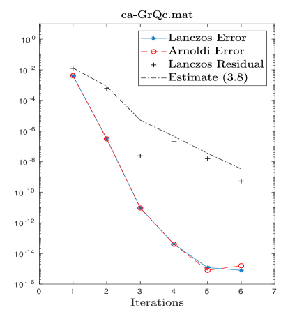
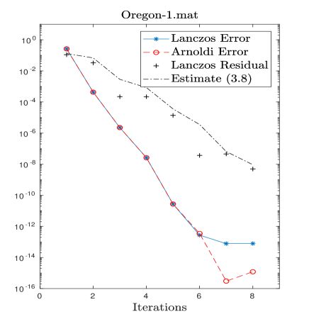
Figure 1: Example 3.2. Convergence history of the Arnoldi error, together with the rational Lanczos error, residual norm (19) for $\tau=1$, and residual estimate (20).

Matrix	size	nnz	Method	It.	Time (secs)
ca-GrQc	5242	28980	$Q_{m}$-less Lanczos	6	0.079
			Rat. Arnoldi	6	0.067
Oregon-1	11492	46818	$Q_{m}$-less Lanczos	8	0.129
			Rat. Arnoldi	8	0.130

Table 1: Example 3.2 with $s=1$. Number of iterations of the $Q_{m}$-less rational Lanczos and Arnoldi methods and corresponding CPU times. Also reported are the dimension and the number of nonzeros (nnz) of each matrix.

Example 3.2.

Let $A$ be the adjacency matrix of a network. For any $i\in\{1,\ldots,n\}$ the quantity $(\exp(A))_{ii}$ measures the importance of the $i$th node with respect to the network edge structure, the so-called $\exp$-centrality index [25]. We consider the symmetric normalized adjacency matrices Oregon-1 and ca-GrQc of size $11492$ and $5242$, respectively, from the SuiteSparse Matrix Collection [16] and the node $i$ with the largest $\exp$-centrality. Both matrices are very sparse, with respectively 4 and 5 elements per row on average. We are interested in approximating the bilinear form $e_{i}^{T}\exp(A-2I)e_{i}$ (note that $\exp(A)=\exp(A-2I)\exp(2)$, with $A-2I$ negative definite). As a quality measure, we use the error between the approximation obtained by the rational Lanczos/Arnoldi methods and the quantity obtained by the matlab function expm.

Figure 1 reports the absolute errors for both approximation methods as the iterations proceed, until the final accuracy is attained after which, not surprisingly, the full orthogonalization approach shows higher accuracy; see, e.g., Figure 1 (right). See also section 4. The figure also shows the norm of the rational Lanczos residual (19) for $\tau=1$ and its estimate (20). In Table 1, we report the number of iterations and corresponding CPU times, confirming the similar behavior of the two approaches, in terms of computational costs. The very limited number of iterations balances the cost of the extra solves in the Lanczos process with that of the full orthogonalization in the Arnoldi iteration.

3.2 The trace of a matrix function

A problem strictly related to that of approximating a quadratic form is given by the approximation of the trace of a matrix function, tr$(f(A))=\sum_{i=1}^{n}(f(A))_{ii}=\sum_{i=1}^{n}f(\lambda_{i})$, where we assume that $A$ is symmetric with eigenvalues $\lambda_{1},\ldots,\lambda_{n}$, and $f(\lambda_{i})$ is well defined for $i=1,\ldots,n$. The approximation of the trace by means of its definition is overly expensive for large matrices, since it requires estimates for $e_{i}^{T}f(A)e_{i}$ for all $i=1,\ldots,n$.

A popular strategy is the use of a Monte-Carlo approximation. Let $Z$ be a discrete random variable with values $\{1,-1\}$ with probability 0.5, and let $z$ be a vector of $n$ independent samples of $Z$. Then $z^{T}f(A)z$ is an unbiased estimator for ${\rm tr}(f(A))$; see, e.g., [37]. By exploiting this result, one can generate $\ell$ sample vectors $z^{(k)}$, $k=1,\ldots,\ell$, estimate $(z^{(k)})^{T}f(A)z^{(k)}\approx\tau_{k}$ by means of the procedure from section 3.1, and obtain

(21) $${\rm tr}(f(A))\approx\frac{1}{\ell}\sum_{k=1}^{\ell}\tau_{k}.$$

For the polynomial Lanczos method and $f(\lambda)=\lambda^{-1}$, this was analyzed in [4]; see also [44]. The effectiveness of the overall approach for general functions of symmetric matrices has been established in [59]; see also [45] for an improved method for stochastic trace approximation, and [15] and its references for general randomized approaches.

In the past few years probing methods have also emerged as an important alternative, especially in network analysis. These differ from Monte-Carlo approximations for the selection of the “probing” vectors $z^{(k)}$, which are then used to estimate $(z^{(k)})^{T}f(A)z^{(k)}$ by means, for instance, of Krylov methods; see, e.g., [27, 8, 45].

In all these strategies, a key step is the use of the Lanczos procedure to obtain an approximation to $(z^{(k)})^{T}f(A)z^{(k)}$; a block method suggests itself. Rational Lanczos can effectively be used to speed up convergence, in terms of number of iterations, with respect to polynomial approaches. A disadvantage of the rational approach lies in the solution of linear systems with the possibly large matrix $I-\xi_{j}^{-1}A$, whose cost depends on the sparsity structure of $A$.

size	$p$	$\delta$	nnz	Method	It.	Time (secs)
1 000	20	0.02	2 260	$Q_{m}$-less Lanczos	6	0.026
				Rat. Arnoldi	6	0.063
		0.06	11 440	$Q_{m}$-less Lanczos	7	0.047
				Rat. Arnoldi	7	0.094
10 000	200	0.002	11 278	$Q_{m}$-less Lanczos	5	1.82
				Rat. Arnoldi	5	1.99
		0.006	21 238	$Q_{m}$-less Lanczos	10	3.76
				Rat. Arnoldi	10	5.96

Table 2: Example 3.3. Number of iterations of the rational Lanczos/Arnoldi method needed to reach the maximal achievable accuracy along with the CPU time in seconds. The approximation space dimension is at most $p\cdot$(# It.+1). nnz refers to the number of nonzero elements in the considered matrices.

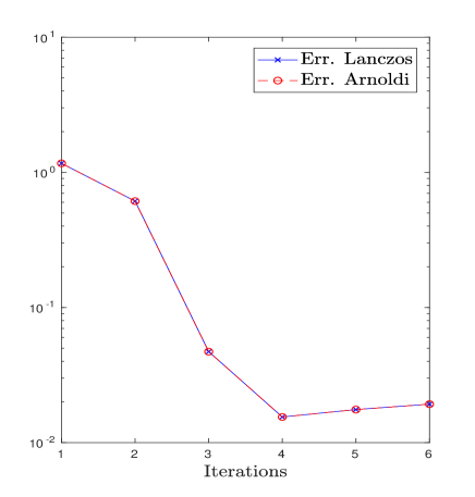
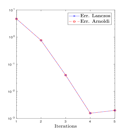
Figure 2: Example 3.3. Convergence error history of the trace estimation (21) obtained at each step of the rational block Lanczos/Arnoldi methods.

Applications related to Gaussian processes often require estimating a parameter $\phi$ by maximizing the so-called log-likelihood function:

(22) $$\log(p\,|\,\phi)=\frac{1}{2}\log\det(A(\phi))-\frac{1}{2}x^{T}A(\phi)x-\frac{n}{2}\log(2\pi),$$

where the positive definite $n\times n$ matrix $A(\phi)$ is the inverse of the covariance matrix parametrized by $\phi$, and $x$ is a given vector; see, e.g., [59]. Estimating $\log\det(A(\phi))$ constitutes the main computational cost in (22). The relation $\log\det(A(\phi))$ $={\rm tr}\log(A(\phi))$ allows one to use the stochastic trace estimator in (21) to reduce the overall computational cost. The values $\tau_{k}$ can be obtained by using the block rational Lanczos algorithm to approximate the bilinear form $B^{T}\log(A(\phi))B$, with $B=[z^{(1)},\dots,z^{(p)}]$.

Example 3.3.

We consider the model in [48]; see also [27]. We generate uniformly distributed random pairs $s_{i}\in[0,1]^{2}$, $i=1,\dots,n$, representing points on the real plane. A random Gaussian variable is associated with each point $s_{i}$. The model describes the association between random variables observed at fixed sites in the Euclidean space, thus imposing a neighborhood structure to the points. More precisely, two points $s_{i},s_{j}$ are associated if and only if the Euclidean distance $d_{ij}=\|s_{i}-s_{j}\|$ is smaller than a given parameter $\delta>0$. Such a structure defines a planar graph. We considered $\phi=20$, while the entries of $A(\phi)$ are defined as follows

$$[A(\phi)]_{ij}=\left\{\begin{array}[]{ll}1+\phi\sum_{k=1,\,k\neq i}^{n}\gamma_{ik},&i=j,\\ -\phi\gamma_{ij},&i\neq j,\end{array}\right.$$

with the so-called reciprocal choice [48]

$$\gamma_{ij}=\left\{\begin{array}[]{ll}1-{d_{ij}}/{\delta},&0<d_{ij}<\delta,\\ 0,&{\rm otherwise}.\end{array}\right.$$

Table 2 reports the results obtained with the $Q_{m}$-less Lanczos and rational Arnoldi algorithms for different values of $n$, $p$, and $\delta$. The sparsity pattern of $A(\phi)$ depends on $\delta$; the larger $\delta$, the denser $A(\phi)$. In spite of the possible cost increase in system solves, the rational Lanczos method turns out to be faster than rational Arnoldi for all the parameters we tested; see Table 2. This may be related to an increased cost of the full orthogonalization step in rational Arnoldi, which seems to suffer the large rank of the matrix $B$. Once again, we used as accuracy measure the error between the computed quantity and the value obtained by means of the matlab logm function.

For each iteration of the rational block Lanczos/Arnoldi algorithm, Figure 2 displays the error in the trace approximation for the rational block Lanczos/Arnoldi algorithms as the iterations proceed. The accuracy reached in the last iterations of the examples agrees with the estimated achievable accuracy of the stochastic strategy we used; see, e.g., [45]. The algorithms behave almost identically in terms of the error.

3.3 $\mathcal{H}_{2}$-norm computation

We consider linear, time-invariant (LTI) systems of the form

(23) $$\Sigma:\left\{\begin{array}[]{l}\dot{x}(t)=Ax(t)+Bu(t),\quad x(0)=x_{0},\\ y(t)=Cx(t),\\ \end{array}\right.$$

where $A\in\mathbb{R}^{n\times n}$ is stable, that is its spectrum is contained in the left-half open complex plane $\mathbb{C}_{-}$, and $B\in\mathbb{R}^{n\times p}$, $C\in\mathbb{R}^{q\times n}$ are low rank, i.e., $p+q\ll n$. The $\mathcal{H}_{2}$-norm of $\Sigma$ is defined as follows

$$\|\Sigma\|^{2}_{\mathcal{H}_{2}}=\text{trace}(C\mathbf{Q}C^{T})=\text{trace}(B^{T}\mathbf{P}B),$$

where $\mathbf{Q}$, $\mathbf{P}\in\mathbb{R}^{n\times n}$ denote the controllability and the observability Gramian, respectively, i.e., $\mathbf{Q}$ and $\mathbf{P}$ are the solution of the following Lyapunov equations

$$A\mathbf{Q}+\mathbf{Q}A^{T}+BB^{T}=0,\quad A^{T}\mathbf{P}+\mathbf{P}A+C^{T}C=0.$$

See, e.g., [3, Section 5.5.1]. The $\mathcal{H}_{2}$-norm gives the maximum amplitude of the system output resulting from input signals of the LTI system (23) with finite energy (see, e.g., [3, 32]), and thus its estimation is of interest.

For $A$ of large dimension $n$, model order reduction (MOR) is used to make the dynamical system numerically tractable [3], so that the $\mathcal{H}_{2}$-norm can also be more cheaply estimated. Given a matrix $Q_{m}$ whose columns span an appropriately chosen reduction space of dimension much lower than $n$, in MOR the following smaller system is introduced,

(24) $$\Sigma_{m}:\left\{\begin{array}[]{ll}\dot{\widehat{x}}(t)=J_{m}\widehat{x}(t)+B_{m}u(t),&\widehat{x}(0)=Q_{m}^{T}x_{0},\;J_{m}=Q_{m}^{T}AQ_{m},\\ \widehat{y}(t)=C_{m}\widehat{x}(t),&B_{m}=Q_{m}^{T}B,\;C_{m}=CQ_{m}.\end{array}\right.\$$

This reduced system is hopefully able to reproduce the main features of the original large scale setting. Rational Krylov subspaces have proven to be particularly effective for this task [3, 7, 28, 31]. For $A$ symmetric, Algorithm 1 produces the small dimensional matrix $J_{m}$, while $B_{m}=Q_{m}^{T}B$ and $C_{m}=CQ_{m}$ can be computed incrementally during the iteration, without explicitly storing $Q_{m}$. After these computations, the $Q_{m}$-less rational Lanczos method can be employed to cheaply compute $\|\Sigma_{m}\|_{\mathcal{H}_{2}}$ as an approximation to $\|\Sigma\|_{\mathcal{H}_{2}}$. In the following we approximate $\|\Sigma\|_{\mathcal{H}_{2}}=\sqrt{\text{trace}(B^{T}\mathbf{P}B)}$ and we thus focus on the approximation of the observability Gramian $\mathbf{P}$. The same procedure can be adopted to compute $\|\Sigma\|_{\mathcal{H}_{2}}=\sqrt{\text{trace}(C\mathbf{Q}C^{T})}$ if the latter formulation is preferred.

The rational Krylov subspace method can also effectively be used for solving the associated Lyapunov equation; see, e.g., [56]. Given the iteratively generated matrix $Q_{m}$ for $\mathcal{K}_{m}(A,C^{T},\bm{\xi})$, an approximation to $\mathbf{P}$ is sought in the form $\mathbf{P}_{m}=Q_{m}Y_{m}Q_{m}^{T}$, where the reduced matrix $Y_{m}$ is obtained by imposing an orthogonality condition on the residual matrix $R_{m}=A\mathbf{P}_{m}+\mathbf{P}_{m}A+C^{T}C$. In terms of the Euclidean matrix inner product, this condition can be written as $Q_{m}^{T}R_{m}Q_{m}=0$. Substituting $\mathbf{P}_{m}$ into the residual and using the orthogonality of the columns in $Q_{m}$ this yields the following reduced Lyapunov equation

$$J_{m}Y_{m}+Y_{m}J_{m}+E_{1}\bm{\gamma\gamma}^{T}E_{1}^{T}=0,$$

where $J_{m}=Q_{m}^{T}AQ_{m}$ and $C^{T}=Q_{1}\bm{\gamma}$ for a nonsigular $\bm{\gamma}\in\mathbb{R}^{q\times q}$. Hence, the small size solution $Y_{m}$ can be computed by means of a Schur decomposition based strategy [56]. Using the computed quantities we can write

$$\|\Sigma\|^{2}_{\mathcal{H}_{2}}= \text{trace}(B^{T}\mathbf{P}B)\approx\text{trace}(B^{T}\mathbf{P}_{m}B)=\text{trace}\left(\left(B^{T}Q_{m}\right)Y_{m}\left(Q_{m}^{T}B\right)\right)=:\|\Sigma_{m}\|^{2}_{\mathcal{H}_{2}}.$$

All the required quantities can be computed without ever storing the whole matrix $Q_{m}$.

Stopping criterion. For the $\mathcal{H}_{2}$-norm computation we propose to check the distance between two subsequent norm approximations, that is, for $1\leq s\leq m-1$,

(25) $$\frac{\left|\|\Sigma_{m}\|_{\mathcal{H}_{2}}-\|\Sigma_{m-s}\|_{\mathcal{H}_{2}}\right|}{\|\Sigma_{m}\|_{\mathcal{H}_{2}}}= \frac{\left|\sqrt{\text{trace}\left(B_{m}^{T}Y_{m}B_{m}\right)}-\sqrt{\text{trace}\left(B_{m-s}^{T}Y_{m-s}B_{m-s}\right)}\right|}{\sqrt{\text{trace}\left(B_{m}^{T}Y_{m}B_{m}\right)}}.$$

The scheme presented in this section can be easily adapted to deal with certain parametric LTI systems like those studied in, e.g., [5], where only the matrices $B=B(\mu)$ and $C=C(\mu)$ affinely depend on a parameter $\mu$ belonging to a given parameter set $\mathcal{D}$.

Example 3.4.

We consider the 2D Optical Tunable Filter dataset available in the MORwiki repository [58] (see also [36]), giving the following LTI system

(26) $$\Sigma:\left\{\begin{array}[]{rcl}E\dot{x}(t)&=&Ax(t)+Bu(t),\\ y(t)&=&Cx(t),\\ \end{array}\right.$$

with $n=1668$, $p=1$, and $q=5$. The mass matrix $E$ is diagonal and positive definite so that we can consider the transformed system

(27) $$\widetilde{\Sigma}:\left\{\begin{array}[]{l}\dot{\widetilde{x}}(t)=\widetilde{A}\widetilde{x}(t)+\widetilde{B}u(t),\\ y(t)=\widetilde{C}\widetilde{x}(t),\\ \end{array}\right.\qquad\begin{array}[]{l}\widetilde{A}=E^{-\frac{1}{2}}AE^{-\frac{1}{2}},\,\widetilde{B}=E^{-\frac{1}{2}}B\\ \widetilde{C}=CE^{-\frac{1}{2}},\,\widetilde{x}=E^{\frac{1}{2}}x.\end{array}$$

This transformation does not affect the $\mathcal{H}_{2}$-norm of the system, since $\|\widetilde{\Sigma}\|_{\mathcal{H}_{2}}=\|\Sigma\|_{\mathcal{H}_{2}}$. We construct $\mathcal{K}_{m}(\widetilde{A},\widetilde{C}^{T},{\bm{\xi}}_{m})$ for the approximation of $\|\widetilde{\Sigma}_{m}\|_{\mathcal{H}_{2}}\approx\|\widetilde{\Sigma}\|_{\mathcal{H}_{2}}$. The iterations are stopped as soon as the relative quantity in (25) for $s=1$ is smaller than $10^{-8}$. Table 3 collects the results for both the $Q_{m}$-less Lanczos and Arnoldi methods, using the same shifts. Thanks to the moderate dimension of the dataset, we are also able to explicitly compute the $\mathcal{H}_{2}$-norm of the full system $\widetilde{\Sigma}$. Therefore, Table 3 also reports the relative error $|\|\widetilde{\Sigma}\|_{\mathcal{H}_{2}}-\|\widetilde{\Sigma}_{m}\|_{\mathcal{H}_{2}}|/\|\widetilde{\Sigma}\|_{\mathcal{H}_{2}}$.

	It.	$\text{dim}\left(\mathcal{K}_{m+1}(\widetilde{A},\widetilde{C}^{T},{\bm{\xi}}_{m+1})\right)$	Time (secs)	Rel. Err.
$Q_{m}$-less Lanczos	12	65	0.219	7.13e-9
Rat. Arnoldi	12	65	0.199	7.13e-9

Table 3: Example 3.4. Results for $Q_{m}$-less rational Lanczos and rational Arnoldi methods to achieve the prescribed accuracy. Shown are number of iterations, space dimension, CPU time and relative error.

The results in Table 3 show a very similar behavior for the $Q_{m}$-less rational Lanczos and rational Arnoldi methods. The Lanczos method allows us to store only 3 basis blocks, namely 15 vectors of length $n$, instead of the whole basis as in the rational Arnoldi method. In terms of CPU time, solving $2q$ linear systems per iteration in the Lanczos approach, instead of only $q$ systems in rational Arnoldi, does not lead to a remarkable increment in the computational efforts.

Example 3.5.

We consider yet another dataset from [58], the 3D Gas Sensor example. The LTI system has the form (26) with a diagonal positive definite mass matrix $E$, hence the transformed LTI system in (27) is employed. In this example we have $n=66917$, $p=1$, and $q=28$. The large problem dimension $n$ does not allow for the computation of the $\mathcal{H}_{2}$-norm of the full system $\widetilde{\Sigma}$, hence only the approximation $\|\widetilde{\Sigma}_{m}\|_{\mathcal{H}_{2}}$ is computed. Since $p$ is significantly smaller than $q$ (the number of columns of $B$ and $C^{T}$, resp.), we proceed by constructing $\mathcal{K}_{m}(\widetilde{A},\widetilde{B},{\bm{\xi}}_{m})$ and then we compute $\|\widetilde{\Sigma}_{m}\|_{\mathcal{H}_{2}}^{2}=\text{trace}(\widetilde{C}\mathbf{\widetilde{Q}}_{m}\widetilde{C}^{T})$. Both methods are stopped as soon as (25) for $s=1$ becomes smaller than $10^{-8}$. Table 4 collects the results. Also for this example the rational Lanczos and Arnoldi methods perform similarly. This means that the cost per iteration of the two schemes is rather similar. On the other hand, for problems where a larger number of iterations is required to converge, the computational cost of the Arnoldi algorithm may significantly increase due to the explicit full orthogonalization.

	It.	$\text{dim}\left(\mathcal{K}_{m+1}(\widetilde{A},\widetilde{B},{\bm{\xi}}_{m+1})\right)$	Time (secs)
$Q_{m}$-less Lanczos	19	20	30.5
Rat. Arnoldi	19	20	28.8

Table 4: Example 3.5. Results for $Q_{m}$-less rational Lanczos and rational Arnoldi methods to achieve the prescribed accuracy. Shown are the number of iterations, the space dimension and the CPU time.

3.4 LQR feedback control

We consider once again LTI systems $\Sigma$ of the form (23), and we investigate the efficient computation of a different quantity related to the so-called linear-quadratic regulator (LQR) problem. Given the LTI system (23) with a stable $A$, this can be stated as

$$u_{*}=\operatorname*{arg\,min}_{u}\mathcal{J}(u),\,\,{\rm with}\,\,\mathcal{J}(u)=\int_{0}^{\infty}y(t)^{T}y(t)+u(t)^{T}R^{-1}u(t)dt,$$

where ${\mathcal{J}}$ is a quadratic cost functional and $R$ is a $p\times p$ symmetric and positive definite matrix. Since $A$ is stable, this $u_{*}$ exists and is given by $u_{*}(t)=-Kx(t)=-R^{-1}B^{T}\mathbf{X}x(t)$, where $\mathbf{X}\in\mathbb{R}^{n\times n}$ is the unique positive semidefinite and stabilizing solution of the following Riccati equation [43]

(28) $$A^{T}\mathbf{X}+\mathbf{X}A-\mathbf{X}BR^{-1}B^{T}\mathbf{X}+C^{T}C=0.$$

Using $u_{*}$ the first equation in (23) can be written in terms of a closed-loop dynamic

$$\dot{x}(t)=(A-BR^{-1}B^{T}\mathbf{X})x(t),\qquad x(0)=x_{0},$$

whose solution is given by $x(t)=\text{exp}((A-BR^{-1}B^{T}\mathbf{X})t)x_{0}$ for $t\geq 0$. Therefore,

(29) $$u_{*}(t)=-R^{-1}B^{T}\mathbf{X}\cdot\text{exp}((A-BR^{-1}B^{T}\mathbf{X})t)x_{0}.$$

In the following we show that for $A$ symmetric an approximation to $u_{*}$ can be cheaply obtained by the $Q_{m}$-less rational Lanczos method; see also [1] for related results.

Rational Krylov subspaces have appeared to lead to competitive methods for solving large-scale Riccati equations; see, e.g., [55] and references therein. In case a projection approach is employed, the overall scheme is very similar to the one reported in section 3.3 for Lyapunov equations. Once again, an approximate solution is sought in the form $\mathbf{X}_{m}=Q_{m}Y_{m}Q_{m}^{T}$, where $\text{Range}(Q_{m})=\mathcal{K}_{m}(A,C^{T},\bm{\xi})$, while $Y_{m}$ is computed, for instance, by imposing an orthogonality (Galerkin) condition on the residual matrix. Explicitly imposing this condition and exploiting the property $Q_{m}^{T}Q_{m}=I$ determines a reduced Riccati equation to be solved in $Y_{m}$ (see [10]), that is

(30) $$J_{m}Y_{m}+Y_{m}J_{m}-Y_{m}B_{m}R^{-1}B_{m}^{T}Y_{m}+E_{1}\bm{\gamma\gamma}^{T}E_{1}=0,$$

where $B_{m}=Q_{m}^{T}B_{m}$ and $\bm{\gamma}\in\mathbb{R}^{q\times q}$ is such that $C^{T}=Q_{1}\bm{\gamma}$. Since $A$ is stable and symmetric, the matrix $J_{m}$ is also stable so that $Y_{m}$ exists and it is the unique positive semidefinite stabilizing solution to (30).

Algorithm 1 can be employed to construct the equation (30) for a growing $m$, where the rows of $B_{m}$ are computed iteratively during the recurrence. At the $m$-th iteration an approximation $u_{m}$ to $u_{*}$ is obtained as

(31) $$u_{m}(t)= R^{-1}B_{m}^{T}Y_{m}\,\,\text{exp}((J_{m}-B_{m}R^{-1}B_{m}^{T}Y_{m})t)(Q_{m}^{T}x_{0})\approx u_{*}(t),$$

which does not require storing the whole $Q_{m}$, since $Q_{m}^{T}x_{0}$ can also be constructed iteratively as $m$ grows. Thanks to the stability of $J_{m}$, it can be shown that the function $u_{m}(t)$ defined in (31) is indeed the optimal control of the reduced model (24), namely ( [55, Corollary 3.2])

$$u_{m}=\operatorname*{arg\,min}_{u}\mathcal{\widehat{J}}(u),\quad\mathcal{\widehat{J}}(u)=\int_{0}^{\infty}\widehat{y}(t)^{T}\widehat{y}(t)+u(t)^{T}R^{-1}u(t)dt.$$

Stopping criterion. The $L^{2}-$distance between two iterates can be employed as a measure to assess the quality of the computed approximation $u_{m}(t)$,

(32) $$\frac{\|u_{m}-u_{m-s}\|_{L^{2}}^{2}}{\|u_{m}\|_{L^{2}}^{2}}=\frac{\int_{0}^{\infty}\|u_{m}(\tau)-u_{m-s}(\tau)\|^{2}d\tau}{\int_{0}^{\infty}\|u_{m}(\tau)\|^{2}d\tau},\quad s\in{\mathbb{N}},\;0<s<m.$$

This quantity can be cheaply approximated because it only involves small dimensional quantities. Furthermore, since $J_{m}-B_{m}R^{-1}B_{m}Y_{m}^{T}$ is a stable matrix, it holds that $\text{exp}((J_{m}-B_{m}R^{-1}B_{m}Y_{m}^{T})t)\rightarrow 0$ as $t\rightarrow\infty$ which may lead to an exponential convergence of the quadrature formula adopted to approximate (32); see, e.g., [12].

Example 3.6.

We consider data in [2, Test 1]. The matrix $A\in\mathbb{R}^{n\times n}$ amounts to the 5-point finite differences discretization of the 2D Laplacian operator in the unit square $[0,1]^{2}$ with zero Dirichlet boundary conditions, namely $A=1/(\bar{n}-1)^{2}\cdot(T\otimes I_{\bar{n}}+I_{\bar{n}}\otimes T)$, $T=\text{tridiag}(1,-2,1)\in\mathbb{R}^{\bar{n}\times\bar{n}}$, $n=\bar{n}^{2}$. The vector $B\in\mathbb{R}^{n}$ is such that the matrix $BB^{T}$ corresponds to the discrete indicating function related to the square $[0.2,0.8]^{2}$. Similarly, $C^{T}C$ with $C\in\mathbb{R}^{1\times n}$ amounts to the discrete indicating function of $[0.1,0.9]^{2}$. We select $R=1$ and $x_{0}=1/(\bar{n}-1)\cdot\mathbf{1}_{n}$ where $\mathbf{1}_{n}\in\mathbb{R}^{n}$ is the vector of all ones.

We compare the $Q_{m}$-less rational Lanczos and Arnoldi methods for the computation of the approximate optimal control $u_{m}(t)$ in (31). Both schemes are stopped as soon as the value in (32) for $s=4$ is smaller than $10^{-8}$. The results in Table 5 show that the two methods perform similarly in terms of convergence trend and computational efficiency. Figure 3 also reports the convergence history of the two schemes for different values of $n$, illustrating that the lack of a full orthogonalization procedure does not affect the convergence of the rational Lanczos method for this example. See section 4 for a broader discussion on this topic.

$n$	It.	$\text{dim}\left(\mathcal{K}_{m+1}(A,C^{T},{\bm{\xi}}_{m+1})\right)$	Method	Time (secs)
40 000	25	26	$Q_{m}$-less Lanczos	2.7
			Rat. Arnoldi	2.6
160 000	29	30	$Q_{m}$-less Lanczos	11.7
			Rat. Arnoldi	11.8
360 000	29	30	$Q_{m}$-less Lanczos	28.3
			Rat. Arnoldi	27.3

Table 5: Example 3.6. Number of iterations of the rational Lanczos/Arnoldi method needed to achieve the prescribed accuracy along with the dimension of the computed subspace and the running time in seconds.

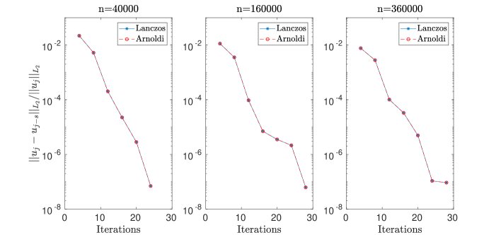
Figure 3: Example 3.6. Convergence history of the rational Lanczos and Arnoldi methods for different values of $n$ and $s=4$.

4 Considerations on finite precision arithmetic computations

The po- lynomial Lanczos iteration is known to be prone to numerical instabilities, which cause loss of orthogonality in the computed basis. This fact has been deeply investigated by Paige in his seminal PhD thesis [46] and successive works, see, e.g., [47]. Quoting [54, p. 108], loss of orthogonality can be viewed as the result of an amplification of each local error after its introduction into the computation, and its growth is determined by the eigenvalue distribution of $A$ and by the starting vector $v$.

The rational Lanczos sequence is tightly related to its polynomial counterpart, with the added difficulty of the system solves, whose finite precision arithmetic computations may significantly increase the perturbation induced by round-off, even assuming a stable direct solver is employed. Notably, to the best of our efforts, we could not find in the literature a round-off errors analysis for rational Krylov subpace computations within the considered applications. In this section we introduce very preliminary considerations on the round-off perturbation occurred in the computed quantities during the iteration. We also report on our numerical experience, showing that the type of loss of orthogonality in the basis seems to be similar to that analyzed in the polynomial Lanczos method over several decades. We are conscious that performing a satisfactory quantitative analysis requires sophisticated tools that go beyond our current presentation. Hopefully, these preliminary results may be useful in a deeper analysis.

At iteration $j$, the generation of the rational Krylov orthonormal basis requires the following computations:

$$\widetilde{r} = Aq_{j}-\beta_{j-1}(I-\xi_{j-2}^{-1}A)q_{j-1},\qquad\widetilde{s}=(I-\xi_{j-1}^{-1}A)q_{j}$$

$$r = (I-\xi_{j}^{-1}A)^{-1}\widetilde{r},\quad s=(I-\xi_{j}^{-1}A)^{-1}\widetilde{s}$$

$$q = r-\alpha_{j}s,\qquad{\rm with}\quad\alpha_{j}=\frac{r^{T}q_{j}}{s^{T}q_{j}}$$

$$q_{j+1} = q/\beta_{j},\quad\beta_{j}=\|q\|.$$

Using standard assumptions on finite precision arithmetic computations, and assuming a backward stable method is used for solving with the symmetric and positive definite matrix $I-\xi_{j}^{-1}A$, we conjecture that an Arnoldi-type relation similar to that in the results of [47] holds, that is

$$AQ_{j}K_{j}=Q_{j}H_{j}+(I-\xi_{j}^{-1}A)q_{j+1}e_{j}^{T}+F_{j},$$

where the matrix $F_{j}$ collects all round-off terms during the iteration. Here we envision that the columns of $F_{j}$ will have an increasing norm as $j$ grows, according with the error accumulation argument known for the polynomial Lanczos. We stress that $K_{j}$ and $H_{j}$ are not the same as those computed in exact arithmetic, and that the columns of $Q_{j}$ are no longer exactly orthonormal, however we can assume that $v=Q_{j}e_{1}$. Although our conjecture seems to be confirmed by numerical experiments, a rigorous analysis leading to upper bounds for the elements in $F_{j}$ would be desirable, though it goes beyond the aim of this work. A different approach to the understanding of the finite precision arithmetic behavior could also follow the backward error analysis introduced by Greenbaum for the Lanczos method [30]. In particular, this approach may enlighten the interplay between the distribution of the eigenvalues of $A$ and the shifts $\xi_{j}$, leading to a better understanding of the rational Lanczos convergence behavior in finite precision arithmetic.

Remark 4.1.

In finite precision it no longer holds that $J_{j}=Q_{j}^{T}AQ_{j}$, and one could even question the symmetry of the computed $J_{j}$. However, since we are mainly concerned with the loss of accuracy in the computation of the length-$n$ vectors, we can assume that $K_{j}^{-1}$ and $J_{j}:=H_{j}K_{j}^{-1}-we^{T}K_{j}^{-1}$ are computed accurately, with $w$ as in the discussion after (7), so that $w^{T}=u^{T}\beta_{j}/\xi_{j}=\beta_{j}/\xi_{j}(\alpha_{j+1}-\eta\beta_{j}/\xi_{j})e_{j}^{T}K_{j}^{-1}=:\upsilon_{j}e_{j}^{T}K_{j}^{-1}$. We thus have

$$J_{j}=(H_{j}-\upsilon_{j}K_{j}^{-T}e_{j}e_{j}^{T})K_{j}^{-1}=H_{j}K_{j}^{-1}-\upsilon_{j}K_{j}^{-T}e_{j}e_{j}^{T}K_{j}^{-1},$$

with $H_{j}K_{j}^{-1}$ symmetric. Hence, $J_{j}$ remains symmetric also in finite precision arithmetic, as long as all quantities are determined using the computed coefficients.

According to Remark 4.1, we thus assume that $J_{j}=H_{j}K_{j}^{-1}-\upsilon_{j}K_{j}^{-T}e_{j}e_{j}^{T}K_{j}^{-1}$ and $K_{j}^{-1}$ are computed exactly. We can then write the perturbed relation as

$$AQ_{j} = Q_{j}H_{j}K_{j}^{-1}+(I-\xi_{j}^{-1}A)q_{j+1}e_{j}^{T}K_{j}^{-1}+F_{j}K_{j}^{-1}$$

$$= Q_{j}J_{j}+[Q_{j}\upsilon_{j}K_{j}^{-T}e_{j}+(I-\xi_{j}^{-1}A)q_{j+1}]e_{j}^{T}K_{j}^{-1}+F_{j}K_{j}^{-1}$$

$$=: Q_{j}J_{j}+z_{j}e_{j}^{T}K_{j}^{-1}+F_{j}K_{j}^{-1}.$$

Subtracting $\zeta Q_{j}$ for $\zeta\in\mathbb{C}$ such that $A-\zeta I$ and $J_{j}-\zeta I$ are nonsingular, we obtain

$$(A-\zeta I)Q_{j}=Q_{j}(J_{j}-\zeta I)+z_{j}e_{j}^{T}K_{j}^{-1}+F_{j}K_{j}^{-1}.$$

Multiplying by $(A-\zeta I)^{-1}$ and $(J_{j}-\zeta I)^{-1}$, and rearranging the relation above we obtain

$$(A-\zeta I)^{-1}Q_{j}=Q_{j}(J_{j}-\zeta I)^{-1}-(A-\zeta I)^{-1}(z_{j}e_{j}^{T}K_{j}^{-1}+F_{j}K_{j}^{-1})(J_{j}-\zeta I)^{-1}.$$

We analyze the effect of this computation in the approximation of the quadratic form $v^{T}f(A)v$, for which the short-term recurrence seems to work particularly well (see section 3.1); see, e.g., [20] for a related analysis of the polynomial Lanczos method. Using $f(A)=\int_{\Gamma}f(\zeta)(A-\zeta I)^{-1}d\zeta$ we can write

$$v^{T}f(A)v = \int_{\Gamma}f(\zeta)v^{T}((A-\zeta I)^{-1}Q_{j})e_{1}d\zeta$$

$$= \int_{\Gamma}f(\zeta)v^{T}Q_{j}(J_{j}-\zeta)^{-1}e_{1}d\zeta$$

$$-v^{T}\int_{\Gamma}f(\zeta)(A-\zeta I)^{-1}(z_{j}e_{j}^{T}+F_{j})K_{j}^{-1}(J_{j}-\zeta I)^{-1}e_{1}d\zeta.$$

Therefore,

$$v^{T}f(A)v=e_{1}^{T}Q_{j}^{T}Q_{j}f(J_{j})e_{1}-v^{T}\int_{\Gamma}f(\zeta)(A-\zeta I)^{-1}(z_{j}e_{j}^{T}+F_{j})K_{j}^{-1}(J_{j}-\zeta I)^{-1}e_{1}d\zeta.$$

In exact arithmetic it would hold that $Q_{j}^{T}Q_{j}=I_{j}$ so that the quantity $e_{1}^{T}f(J_{j})e_{1}$ would correspond to the classical approximation in the given subspace. In finite precision arithmetic the distance from the ideal quantity can be estimated as follows

$$|v^{T}f(A)v-e_{1}^{T}f(J_{j})e_{1}| \leq |e_{1}^{T}f(J_{j})e_{1}-q_{1}^{T}Q_{j}f(J_{j})e_{1}|$$

$$+\left|\int_{\Gamma}f(\zeta)v^{T}(A-\zeta I)^{-1}z_{j}e_{j}^{T}K_{j}^{-1}(J_{j}-\zeta I)^{-1}e_{1}d\zeta\;\right|$$

$$+\left|\int_{\Gamma}f(\zeta)v^{T}(A-\zeta I)^{-1}F_{j}K_{j}^{-1}(J_{j}-\zeta I)^{-1}e_{1}d\zeta\;\right|$$

$$=: \mathcal{I}+\mathcal{I}\mathcal{I}+\mathcal{I}\mathcal{I}\mathcal{I}.$$

We next analyze the right-hand side terms. Let $q_{1}^{T}Q_{j}=e_{1}+\bm{\epsilon}_{j}$, where we can assume that $e_{1}^{T}\bm{\epsilon}_{j}=0$ (exact normalization) while the quantity $|e_{k}^{T}\bm{\epsilon}_{j}|$ may grow with $k$. Then

(33) $$|e_{1}^{T}f(J_{j})e_{1}-q_{1}^{T}Q_{j}f(J_{j})e_{1}| = |{\bm{\epsilon}}_{j}^{T}f(J_{j})e_{1}|$$

$$= |\sum_{\ell=1}^{j}({\bm{\epsilon}}_{j})_{\ell}(f(J_{j})e_{1})_{\ell}|\leq\sum_{\ell=1}^{j}|({\bm{\epsilon}}_{j})_{\ell}|\,|(f(J_{j})e_{1})_{\ell}|.$$

In exact arithmetic, it has been proved that $|e_{\ell}^{T}f(J_{j})e_{1}|$ shows a decaying behavior - which is possibly exponential - as $\ell$ grows, and the slope depends on the spectral properties of the coefficient matrix [49]. If this property is maintained in finite precision arithmetic, then each term $|({\bm{\epsilon}}_{j})_{\ell}|$ is allowed to grow as long as the product $|({\bm{\epsilon}}_{j})_{\ell}|\,|(f(J_{j})e_{1})_{\ell}|$ remains small.

Assuming that $K_{j}$ is computed exactly, the term $\mathcal{I}\mathcal{I}$ does not involve perturbation matrices, therefore its magnitude is related to the quality of the rational Krylov space approximation in exact precision arithmetic. Lastly, the term $\mathcal{I}\mathcal{I}\mathcal{I}$ shows that the columns of the round-off error matrix are weighted by the components of the vector $K_{j}^{-1}(J_{j}-\zeta I)^{-1}e_{1}$. By using the definition of $J_{j}$ and $K_{j}$, it follows that $(J_{j}-\zeta I)K_{j}=H_{j}-\zeta K_{j}-w_{j}e_{j}^{T}$, which is a tridiagonal plus a rank-one matrix acting on the last column. Setting $G_{j}=H_{j}-\zeta K_{j}$ with $G_{j}=G_{j}(\zeta)$ and using the Sherman-Morrison formula, we get $K_{j}^{-1}(J_{j}-\zeta I)^{-1}e_{1}=G_{j}^{-1}e_{1}+G_{j}^{-1}w_{j}(e_{j}^{T}G_{j}^{-1}e_{1})/(1-e_{j}^{T}G_{j}^{-1}w)$. If $G_{j}$ has convenient spectral properties, then the components of the vector $G_{j}^{-1}e_{1}$ have a decaying magnitude, while the magnitude of the second term in the formula depends on $e_{j}^{T}G_{j}^{-1}e_{1}$, the last component of the first vector. Hence, in this case the propagated errors contained in the rightmost columns of $F_{j}$ are weighted by small values. As a consequence, the round-off effect appears to be mitigated. Although we have experimental evidence that round-off errors seem to only slightly affect computations, a thorough analysis is needed to make more definitive statements.

Remark 4.2.

For $f(z)=z^{-1}$ the polynomial Lanczos analysis is closely related to that of the conjugate gradient (CG) method for solving linear systems. We refer the reader to the monograph [41] and its references for a thorough discussion.

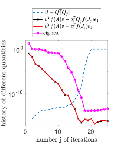
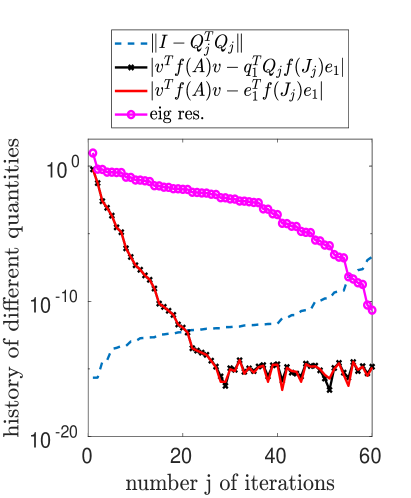
Figure 4: Example 4.3. Convergence history of approximation to $v^{T}A^{1/2}v$. Left: $\rho=0.45$. Right: $\rho=0.85$.

Example 4.3.

We consider an example first introduced in [57]. The matrix is diagonal with eigenvalues equal to $\lambda_{i}=\lambda_{1}+(i-1)/(n-1)(\lambda_{1}-\lambda_{n})\rho^{n-i}$, $i=1,\ldots,n$; the parameter $\rho$ is used to control the eigenvalue distribution in the spectral interval, so that a value of $\rho$ close to one distributes the eigenvalues almost uniformly in the interval. We considered $n=900$, $\lambda_{1}=0.01$ and $\lambda_{n}=100$, together with $f(\lambda)=\lambda^{1/2}$. Moreover, we analyzed two values of $\rho$, that is $\rho=0.45$ and $\rho=0.85$. The plots in Figure 4 show the error $|v^{T}f(A)v-e_{1}^{T}f(J_{j})e_{1}|$ together with the loss of orthogonality $\|I-Q_{j}^{T}Q_{j}\|$ and the true approximation error $|v^{T}f(A)v-q_{1}^{T}Q_{j}f(J_{j})e_{1}|$ as the number $j$ of iterations increases. Plots are reported for $\rho=0.45$ (left) and $\rho=0.85$ (right). The eigenvalue residual norm $\|Ax^{(j)}-x^{(j)}\lambda^{(j)}\|/|\lambda^{(j)}|$ is also shown, where $(\lambda^{(j)},x^{(j)})$ is the Ritz eigenpair with $\lambda^{(j)}$ closest to $\lambda_{n}$. Similarly to the polynomial Lanczos method, for both values of $\rho$ loss of orthogonality is related to the convergence of the Ritz eigenpair to the corresponding eigenpair of $A$. Concerning the bilinear form, we first remark that the convergence to $v^{T}f(A)v$ is not consistently related to that of the Ritz eigenpair, and in addition convergence seems to be insensitive to the fact that $q_{1}^{T}Q_{j}\neq e_{1}$, that is, ${\bm{\epsilon}}_{j}\neq 0$. Though convergence is slower for $\rho=0.85$ than for $\rho=0.45$, the last property is maintained in both cases.

In the previous example we illustrated that the accuracy obtained by $q_{1}^{T}Q_{j}f(J_{j})e_{1}$ is similar to that of $e_{1}^{T}f(J_{j})e_{1}$, and this is related to the role of $|\sum_{\ell=1}^{j}({\bm{\epsilon}}_{j})_{\ell}(f(J_{j})e_{1})_{\ell}|$ in the discussion above. The next example investigates this issue further.

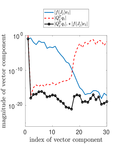
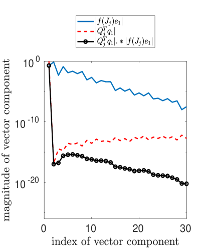
Figure 5: Example 4.4. Magnitude of components at iteration $j=30$ in the approximation to $v^{T}A^{1/2}v$. Left: $\rho=0.45$. Right: $\rho=0.85$.

Example 4.4.

With the same data as in Example 4.3, we focus on iteration $j=30$ and inspect the magnitude of the components of the vectors $f(J_{j})e_{1}$ and $q_{1}^{T}Q_{j}$, which give the factors in the sum $|\sum_{\ell=1}^{j}({\bm{\epsilon}}_{j})_{\ell}(f(J_{j})e_{1})_{\ell}|$. The two plots in Figure 5 ($\rho=0.45$ on the left and $\rho=0.85$ on the right) report the quantities $|f(J_{j})e_{1}|_{\ell}$, $|q_{1}^{T}Q_{j}|_{\ell}$ and $|q_{1}^{T}Q_{j}|_{\ell}|f(J_{j})e_{1}|_{\ell}$ for $\ell=1,\ldots,30$. The two figures consistently report that the increasing pattern of $|q_{1}^{T}Q_{j}|_{\ell}$ inversely matches the decreasing one of $|f(J_{j})e_{1}|_{\ell}$, so that the product of each component remains at the level of $10^{-15}$. If $J_{j}$ were exact, the decay pattern of $|f(J_{j})e_{1}|_{\ell}$ would be expected, thanks to the theoretical results reported in [49]. The fact that round-off error does not seem to significantly alter the interplay between $|q_{1}^{T}Q_{j}|_{\ell}$ and $|f(J_{j})e_{1}|_{\ell}$ could be related to the theory developed by Greenbaum [30]. For the polynomial Lanczos method, Greenbaum showed that the computed projected matrix can be expressed as the output of the Lanczos iteration applied in exact arithmetic not to $A$ but to a matrix $\tilde{A}$ of larger dimensions. In particular the eigenvalues of $\tilde{A}$ cluster around those of $A$. If an analogous result could be derived for the projected matrix $J_{j}$ computed by the rational Lanczos method, then the result in [49] would ensure that the decay pattern of $|f(J_{j})e_{1}|_{\ell}$ also holds in finite precision. This would justify the persistency of the interplay between $|q_{1}^{T}Q_{j}|_{\ell}$ and $|f(J_{j})e_{1}|_{\ell}$ in finite precision arithmetic. We will address this intriguing issue in future research.

4.1 Stability of the LU factorization of $K_{j}$

In section 2.1 it was stated that the LU factorization $K_{j}=L_{j}U_{j}$ with no pivoting exists. In this section we analyze its stability properties. Assuming that $K_{j}$ is computed exactly, the stability of the LU factorization will ensure that the recurrences (9) and (10) are backward stable. To this end, we write

$$K_{j}=\begin{bmatrix}1&0\\ \frac{\beta_{1}}{\xi_{1}}&\widetilde{K}_{j}\end{bmatrix}\quad{\rm with}\,\,\widetilde{K}_{j}=\widetilde{D}_{j-1}^{-1}\widetilde{T}_{j},\quad\widetilde{T}_{j}:=\begin{bmatrix}\xi_{1}+{\alpha_{2}}&{\beta_{2}}\\ {\beta_{2}}&\xi_{2}+{\alpha_{3}}&\hskip 2.0pt\ddots&\\ &\ddots&\ddots&{\beta_{j-1}}\vspace{4pt}\\ &&{\beta_{j-1}}&\xi_{j-1}+{\alpha_{j}}\vspace{4pt}\end{bmatrix},$$

where $\widetilde{T}_{j}\in\mathbb{R}^{(j-1)\times(j-1)}$ and $\widetilde{D}_{j-1}:=\text{diag}(\xi_{1},\dots,\xi_{j-1})$.

Lemma 4.5.

Let $j_{*}\leq n$ be the first index such that $\beta_{j_{*}}=0$, giving subspace invariance in (4). Using the notation of Section 2.1, let $A$ be symmetric and positive definite, and the shifts $\xi_{1},\ldots,\xi_{j_{*}-1}$ all be negative. Then the symmetric matrices $H_{j}$ and $\widetilde{T}_{j}$ are both positive definite, for $j\leq j_{*}$. Vice-versa, if $A$ is symmetric and negative definite with positive shifts, then $H_{j}$ is negative definite while $\widetilde{T}_{j}$ is positive definite.

Proof 4.6.

We prove the result for $A$ negative definite; the positive definite case follows similarly. We have $J_{j_{*}}=H_{j_{*}}K_{j_{*}}^{-1}$ so that $J_{j_{*}}K_{j_{*}}=J_{j_{*}}+J_{j_{*}}D_{{j_{*}}-1}^{-1}H_{j_{*}}=H_{j_{*}}$, from which

$$H_{j_{*}}=(I_{j_{*}}-J_{j_{*}}D_{{j_{*}}-1}^{-1})^{-1}J_{j_{*}}=(J_{j_{*}}^{-1}-D_{{j_{*}}-1}^{-1})^{-1}.$$

Since $J_{j_{*}}=Q_{j_{*}}^{T}AQ_{j_{*}}$ is symmetric and negative definite, and the shifts are all positive, it follows that $H_{j_{*}}$ is a negative definite matrix. Moreover, the eigenvalues of $K_{j_{*}}$ are positive since $K_{j_{*}}=H_{j_{*}}J_{j_{*}}^{-1}$ is the product of two symmetric negative definite matrices.

For any $j\leq{j_{*}}$, the eigenvalues of $H_{j}$ are contained in the spectral interval of $H_{j_{*}}$, so that $H_{j}$ is positive definite. To derive the positive definiteness of $\widetilde{T}_{j}$, we observe that for any $j\leq{j_{*}}$, the spectrum of $K_{j}$ is composed of $1$ and all the eigenvalues of the submatrix $\widetilde{K}_{j}=\widetilde{D}_{j-1}^{-1}\widetilde{T}_{j}$, with $j\leq{j_{*}}$. For $j=j_{*}$, the positivity of the eigenvalues of $K_{j_{*}}$ ensures that of the eigenvalues of $\widetilde{K}_{j_{*}}$. In particular, since $\widetilde{D}_{j_{*}-1}>0$, this implies that $\widetilde{T}_{j_{*}}$ is positive definite. Hence, all principal $j\times j$ matrices of $\widetilde{T}_{j_{*}}$ are also positive definite, with $j\leq{j_{*}}$.

We can prove the backward stability of the Gaussian elimination procedure associated with $K_{j}$, thus proving Proposition 2.4. Here $|M|$ is the matrix obtained by taking the element-wise absolute values of the matrix $M$.

Proposition 4.7.

Under the assumptions of Lemma 4.5, if the unit roundoff u is small enough, then the Gaussian elimination for the system $K_{j}y=e_{j}$ succeeds, and the computed solution $\hat{y}$ satisfies

$$(K_{j}+\Delta K_{j})\hat{y}=e_{j},\quad|\Delta K_{j}|<h({\tt u})|K_{j}|,\quad h({\tt u})=\frac{4{\tt u}+3{\tt u}^{2}+{\tt u}^{3}}{1-{\tt u}}.$$

The same holds for the system $K_{j}^{T}t=e_{j}$.

Proof 4.8.

Following the argument in [35, section 9.6], it is sufficient to prove that the LU factorization $K_{j}=L_{j}U_{j}$ satisfies $|L_{j}||U_{j}|=|L_{j}U_{j}|$ with $U_{j}$ having positive diagonal elements, and the result will follow from [35, Theorem 9.14] and its proof. We restrict our attention to the matrix $\widetilde{K}_{j}$, as the first row and column of $K_{j}$ are already in the desired form.

For $A$ negative definite, from Lemma 4.5 it follows that the matrix $\widetilde{T}_{j}=\widetilde{D}_{j-1}\widetilde{K}_{j}$ is positive definite. In particular, Theorem 9.12 in [35] ensures that the LU factorization $\widetilde{T}_{j}=\widetilde{L}_{j}\widetilde{U}_{j}$ satisfies the condition $|\widetilde{L}_{j}||\widetilde{U}_{j}|=|\widetilde{L}_{j}\widetilde{U}_{j}|$. Therefore, the matrix $\widetilde{K}_{j}$ can be factorized as $\widetilde{K}_{j}=\widetilde{D}_{j-1}^{-1}\widetilde{L}_{j}\widetilde{U}_{j}$. Note that the matrix $\widehat{L}_{j}:=\widetilde{D}_{j-1}^{-1}\widetilde{L}_{j}\widetilde{D}_{j-1}$ is lower bidiagonal with all the diagonal entries equal to $1$. Then

$$\widetilde{K}_{j}=\widehat{L}_{j}\widetilde{D}_{j-1}^{-1}\widetilde{U}_{j}=\widehat{L}_{j}\widehat{U}_{j},$$

is the unique LU factorization of $\widetilde{K}_{j}$, with $\widehat{U}_{j}:=\widetilde{D}_{j-1}^{-1}\widetilde{U}_{j}$. Note that the diagonal elements of $\widehat{U}_{j}$ are positive. Since $\widetilde{D}_{j-1}$ has positive diagonal entries, we get the following equalities

$$|\widehat{L}_{j}||\widehat{U}_{j}| =|\widehat{L}_{j}||\widetilde{D}_{j-1}^{-1}\widetilde{U}_{j}|=|\widehat{L}_{j}\widetilde{D}_{j-1}^{-1}||\widetilde{U}_{j}|=|\widetilde{D}_{j-1}^{-1}\widetilde{L}_{j}||\widetilde{U}_{j}|=|\widetilde{D}_{j-1}^{-1}||\widetilde{L}_{j}||\widetilde{U}_{j}|$$

$$=|\widetilde{D}_{j-1}^{-1}||\widetilde{L}_{j}\widetilde{U}_{j}|=|\widetilde{D}_{j-1}^{-1}\widetilde{L}_{j}\widetilde{U}_{j}|=|\widehat{L}_{j}\widehat{U}_{j}|.$$

Returning to $K_{j}$, and using the notation of the proof of Lemma 2.1, we observe that the first two computed coefficients in the factorization $K_{j}=L_{j}U_{j}$ are $\omega_{1}=1$ and $\ell_{2}=\beta_{1}/\xi_{1}>0$. Hence, it holds that $|L_{j}||U_{j}|=|L_{j}U_{j}|$ with $U_{j}$ having positive diagonal elements, concluding the proof.

The case in which $A$ is positive definite can be proved analogously.

5 Conclusions

We have described a computationally and memory efficient implementation of the symmetric rational Lanczos method. The algorithm does not require storing the whole orthonormal basis $Q_{m}$ to proceed with the iterations. We have illustrated a number of application problems where the proposed $Q_{m}$-less algorithm can effectively be employed. Very preliminary considerations of finite precision arithmetic computations seem to indicate that the behavior of the short-term recurrence rational method in this context is similar to that of its polynomial counterpart, although a comprehensive analysis is required to make more definitive statements.

Appendix

In this section we present the block variant of Algorithm 1.

input : $A\in\mathbb{R}^{n\times n}$, $V\in\mathbb{R}^{n\times p}$, $\bm{\xi}$, number of iterations $m>0$.

output : $J_{m}\in\mathbb{R}^{pm\times pm}$, $J_{m}=Q_{m}^{T}AQ_{m}$, $\text{Range}(Q_{m})={\cal K}_{m}(A,V,\bm{\xi}_{m})$.

1 Compute a skinny QR factorization of $V$, $\widehat{Q}\widehat{R}=V$

2

3while $j\leq m$ do

4       if $j=1$ then

5             Set $\widetilde{R}=A\widehat{Q}$ and $\widetilde{S}=\widehat{Q}$

6            

7      else if $j=2$ then

8             Set $\widetilde{R}=A\widehat{Q}-\bar{Q}\beta_{j-1}^{T}$ and $\widetilde{S}=(I-A/\xi_{j-1})\widehat{Q}$

9      else

10             Set $\widetilde{R}=A\widehat{Q}-(I-A/\xi_{j-2})\bar{Q}\beta_{j-1}^{T}$ and $\widetilde{S}=(I-A/\xi_{j-1})\widehat{Q}$

11      Solve $(I-A/\xi_{j})[R,S]=[\widetilde{R},\widetilde{S}]$

12      

13      Compute $\alpha_{j}=\left(\widehat{Q}^{T}S\right)^{-1}\left(\widehat{Q}^{T}R\right)$

14      

15      Set $Q=R-S\alpha_{j}$

16      

17      Set $\bar{Q}=\widehat{Q}$

18      

19      Compute a skinny QR factorization of $Q$, $\widehat{Q}\beta_{j}=Q$

20      

21      if j=1 then

22             Set $u_{j}=y_{1}=t_{1}=I_{p}$ and $\widehat{y}_{1}=\alpha_{1}$

23      else

24             Set $u_{j}=\alpha_{j}/\xi_{j-1}+I_{p}-\beta_{j-1}\omega_{j-1}^{-1}\beta_{j-1}^{T}/(\xi_{j-1}\xi_{j-2})$

25            

26            Set $y_{j}=\begin{bmatrix}-y_{j-1}\beta_{j-1}^{T}\omega_{j}^{-1}/\xi_{j-2}\\ \omega_{j}^{-1}\\ \end{bmatrix}$, $t_{j}=\begin{bmatrix}-t_{j-1}\beta_{j-1}^{T}\omega_{j}^{-1}/\xi_{j-1}\\ \omega_{j}^{-1}\\ \end{bmatrix}$, and $\widehat{y}_{j}=\begin{bmatrix}-\widehat{y}_{j-1}\beta_{j-1}^{T}\omega_{j}^{-1}/\xi_{j-2}\\ \beta_{j-1}^{T}E_{j-1}^{T}y_{j}+\alpha_{j}\omega_{j}^{-1}\\ \end{bmatrix}+E_{j-1}\beta_{j-1}u_{j}^{-1}$

27      Compute $\eta=\widehat{Q}^{T}A\widehat{Q}$

28      

29      Set $J_{j}E_{j}=\widehat{y}_{j}-t_{j}\beta_{j}^{T}(I_{p}-\eta/\xi_{j})\beta_{j}/\xi_{j}u_{j}^{-1}$ and $E_{j}^{T}J_{j}=(J_{j}E_{j})^{T}$

30      

31      Set $j=j+1$

Algorithm 2 Block rational Lanczos.

References

- [1] A. Alla, D. Kalise, and V. Simoncini, State-dependent Riccati Equation Feedback Stabilization for Nonlinear PDEs, June 2021. Preprint ArXiv: x2106.07163.
- [2] A. Alla and V. Simoncini, Order Reduction Approaches for the Algebraic Riccati Equation and the LQR Problem, in Numerical Methods for Optimal Control Problems, vol. 29 of Springer INdAM Series, 2018, pp. 89–109.
- [3] A. C. Antoulas, Approximation of Large-Scale Dynamical Systems, SIAM, Philadelphia, 2005.
- [4] Z. Bai, G. Fahey, and G. Golub, Some Large-scale Matrix Computation Problems, J. Comput. Appl. Math., 74 (1996), pp. 71–89.
- [5] U. Baur, C. Beattie, P. Benner, and S. Gugercin, Interpolatory Projection Methods for Parameterized Model Reduction, SIAM J. Sci. Comput., 33 (2011), pp. 2489–2518.
- [6] B. Beckermann and L. Reichel, Error Estimates and Evaluation of Matrix Functions via the Faber Transform, SIAM J. Numer. Anal., 47 (2009), pp. 3849–3883.
- [7] P. Benner, A. Cohen, M. Ohlberger, and K. Willcox, Model Reduction and Approximation: Theory and Algorithms, Computational Science & Engineering, SIAM, Philadelphia, 2017.
- [8] A. H. Bentbib, M. El Ghomari, K. Jbilou, and L. Reichel, Shifted Extended Global Lanczos Processes for Trace Estimation with Application to Network Analysis, Calcolo, 58 (2021).
- [9] M Benzi and G. H. Golub, Bounds for the Entries of Matrix Functions with Applications to Preconditioning, BIT, 39 (1999), pp. 417–438.
- [10] D.A. Bini, B. Iannazzo, and B. Meini, Numerical Solution of Algebraic Riccati Equations, SIAM, Philadelphia, 2012.
- [11] M.A. Botchev, V. Grimm, and M. Hochbruck, Residual, Restarting and Richardson Iteration for the Matrix Exponential, SIAM J. Sci. Comp., 35 (2013), pp. A1376–A1397.
- [12] J.P. Boyd, Exponentially Convergent Fourier-Chebyshev Quadrature Schemes on Bounded and Infinite Intervals, J. Sci. Comput., 2 (1987), p. 99–109.
- [13] A. Bultheel, P. Gonzalez-Vera, E. Hendriksen, and O. Njastad, Orthogonal Rational Functions and Tridiagonal Matrices, J. Comput. Applied Math., 153 (2003), pp. 89–97.
- [14] J. Chen and Y. Saad, A Posteriori Error Estimate for Computing tr(f(A)) by Using he Lanczos Method, Num. Linear Algebra Appl., 25 (2018), p. e2170.
- [15] A. Cortinovis and D. Kressner, On Randomized Trace Estimates for Indefinite Matrices with an Application to Determinants, Found. Comput. Math., (2021).
- [16] T. A. Davis and Y. Hu, The University of Florida Sparse Matrix Collection, ACM Trans. Math. Software, 38 (2011), pp. 1–25.
- [17] B. de la Calle Ysern, Error Bounds for Rational Quadrature Formulae of Analytic Functions, Numer. Math., 101 (2005), pp. 251–271.
- [18] K. Deckers and A. Bultheel, Rational Krylov Sequences and Orthogonal Rational Functions, tech. report, Department of Computer Science, K.U.Leuven, 2007.
- [19] K. Deckers and A. Bultheel, The Existence and Construction of Rational Gauss-type Quadrature Rules, Applied Math. and Comput., 218 (2012), pp. 10299–10320.
- [20] V. Druskin, A. Greenbaum, and L. Knizhnerman, Using Nonorthogonal Lanczos Vectors in the Computation of Matrix Functions, SIAM J. Sci. Comput., 19 (1998), pp. 38–54.
- [21] V. Druskin, L. Knizhnerman, and V. Simoncini, Analysis of the Rational Krylov Subspace and ADI Methods for Solving the Lyapunov Equation, SIAM J. Numer. Anal., 49 (2011), pp. 1875–1898.
- [22] V. Druskin, L. Knizhnerman, and M. Zaslavsky, Solution of Large Scale Evolutionary Problems Using Rational Krylov Subspaces with Optimized Shifts, SIAM J. Sci. Comput., 31 (2009), pp. 3760–3780.
- [23] V. Druskin, C. Lieberman, and M. Zaslavsky, On Adaptive Choice of Shifts in Rational Krylov Subspace Reduction of Evolutionary Problems, SIAM J. Sci. Comput., 32 (2010), pp. 2485–2496.
- [24] V. Druskin and V. Simoncini, Adaptive Rational Krylov Subspaces for Large-scale Dynamical Systems, Systems Control Lett., 60 (2011), pp. 546–560.
- [25] E. Estrada and J. A. Rodríguez-Velázquez, Subgraph Centrality in Complex Networks, Phys. Rev. E, 71 (2005), p. 056103.
- [26] C. Fenu, L. Reichel, and G. Rodriguez, GCV for Tikhonov Regularization via Global Golub–Kahan Decomposition, Numer. Linear Algebra Appl., 23 (2016), pp. 467–484.
- [27] A. Frommer, C. Schimmel, and M. Schweitzer, Analysis of Probing Techniques for Sparse Approximation and Trace Estimation of Decaying Matrix Functions, SIAM J. Matrix Anal. Appl., 42 (2021), pp. 1290–1318.
- [28] K. Gallivan, E. Grimme, and P. Van Dooren, A Rational Lanczos Algorithm for Model Reduction, Numer. Algorithms, 12 (1996), pp. 33–63.
- [29] G. H. Golub and G. Meurant, Matrices, Moments and Quadrature with Applications, Princeton University Press, Princeton, 2010.
- [30] A. Greenbaum, Behavior of Slightly Perturbed Lanczos and ConJugate-Gradient Recurrences, Linear Algebra Appl., 113 (1989), pp. 7–63.
- [31] E. Grimme, Krylov Projection Methods for Model Reduction, PhD thesis, The University of Illinois at Urbana-Champaign, 1997.
- [32] S. Gugercin, A. C. Antoulas, and C. Beattie, Model Reduction for Large-Scale Linear Dynamical Systems, SIAM J. Matrix Anal. Appl., 30 (2008), pp. 609–638.
- [33] S. Güttel, Rational Krylov Methods for Operator Functions, PhD thesis, TU Bergakademie Freiberg, Germany, 2010.
- [34] S. Güttel, Rational Krylov Approximation of Matrix Functions: Numerical Methods and Optimal Pole Selection, GAMM-Mitteilungen, 36 (2013), pp. 8–31.
- [35] N. J. Higham, Accuracy and Stability of Numerical Algorithms, SIAM, Philadelphia, PA, second ed., 2002.
- [36] D. Hohlfeld and H. Zappe, An All-dielectric Tunable Optical Filter Based on the Thermo-optic Effect, J. Opt. A: Pure Appl. Opt., 6 (2004), pp. 504–511.
- [37] M. Hutchinson, A Stochastic Estimator of the Trace of the Influence Matrix for Laplacian Smoothing Splines, Comm. Statist. Simul., 18 (1989), pp. 1059–1076.
- [38] L. Knizhnerman and V. Simoncini, A New Investigation of the Extended Krylov Subspace Method for Matrix Function Evaluations, Numer. Linear Algebra Appl., 17 (2010), pp. 615–638.
- [39] J. V. Lambers, Solution of Time-dependent PDE through Component-wise Approximation of Matrix Functions, IAENG Int. J. Appl. Math., 41 (2011), pp. 1–10.
- [40] C. Lanczos, Solution of Linear Equations by Minimized Iterations, J. Res. Natl. Bur. Stand., 49 (1952), pp. 33–53.
- [41] J. Liesen and Z. Strakoš, Krylov Subspace Methods: Principles and Analysis, Oxford University Press, Oxford, 2013.
- [42] The MathWorks, Inc., MATLAB, http://www.matlab.com.
- [43] V. L. Mehrmann, The Autonomous linear Quadratic Control Problem: Theory and Numerical Solution, vol. 163 of Lecture Notes in Control and Information Sciences, Springer-Verlag, Berlin, 1991.
- [44] G. Meurant, Estimates of the Trace of the Inverse of a Symmetric Matrix Using the Modified Chebyshev Algorithm, Numer. Algorithms, 51 (2009), pp. 309–318.
- [45] R. A. Meyer, C. Musco, C. Musco, and D. P. Woodruff, Hutch++: Optimal Stochastic Trace Estimation, in Symposium on Simplicity in Algorithms (SOSA), Society for Industrial and Applied Mathematics, January 2021, pp. 142–155.
- [46] C. C. Paige, The Computation of Eigenvalues and Eigenvectors of Very Large and Sparse Matrices, PhD thesis, London University, London, England, 1971.
- [47] , Error Analysis of the Lanczos Algorithm for Tridiagonalizing a Symmetric Matrix, J. Inst. Math. Appl., 18 (1976), pp. 341–349.
- [48] A. N. Pettitt, I. S. Weir, and A. G. Hart, A Conditional Autoregressive Gaussian Process for Irregularly Spaced Multivariate Data with Application to Modelling Large Sets of Binary Data, Stat. Comput., 12 (2002), pp. 353–367.
- [49] S. Pozza and V. Simoncini, Functions of Rational Krylov Space Matrices and their Decay Properties, Numer. Math., 148 (2021), p. 99–126.
- [50] M. S. Pranić and L. Reichel, Rational Gauss Quadrature, SIAM J. Numer. Anal., 52 (2014), pp. 832–851.
- [51] A. Ruhe, Rational Krylov Sequence Methods for Eigenvalue Computation, Lin. Alg. Appl., 58 (1984), pp. 391–405.
- [52] Y. Saad, J. R. Chelikowsky, and S. M. Shontz, Numerical Methods for Electronic Structure Calculations of Materials, SIAM Review, 52 (2010), pp. 3–54.
- [53] M. Schweitzer, Monotone Convergence of the Extended Krylov Subspace Method for Laplace–Stieltjes Functions of Hermitian Positive Definite Matrices, Linear Algebra Appl., 507 (2016), pp. 486–498.
- [54] H. D. Simon, Analysis of the Symmetric Lanczos Algorithm with Reorthogonalization Methods, Linear Algebra Appl., 61 (1984), pp. 101–131.
- [55] V. Simoncini, Analysis of the Rational Krylov Subspace Projection Method for Large-scale Algebraic Riccati Equations, SIAM J. Matrix Anal. Appl., 37 (2016), pp. 1655–1674.
- [56] , Computational Methods for Linear Matrix Equations, SIAM Review, 58 (2016), pp. 377–441.
- [57] Z. Strakoš, On the Real Convergence Rate of the Conjugate Gradient Method, Linear Algebra Appl., 15–156 (1991), pp. 53–549.
- [58] The MORwiki Community, MORwiki - Model Order Reduction Wiki. http://modelreduction.org.
- [59] S. Ubaru, J. Chen, and Y. Saad, Fast Estimation of tr(f(A)) via Stochastic Lanczos Quadrature, SIAM J. Matrix Anal. Appl., 38 (2017), pp. 1075–1099.
- [60] N. Van Buggenhout, M. Van Barel, and R. Vandebril, Biorthogonal Rational Krylov Subspace Methods, Electron. Trans. Numer. Anal., 51 (2019), pp. 451–468.