\ul
NVUM: Non-Volatile Unbiased Memory for Robust Medical Image Classification
Abstract
Real-world large-scale medical image analysis (MIA) datasets have three challenges: 1) they contain noisy-labelled samples that affect training convergence and generalisation, 2) they usually have an imbalanced distribution of samples per class, and 3) they normally comprise a multi-label problem, where samples can have multiple diagnoses. Current approaches are commonly trained to solve a subset of those problems, but we are unaware of methods that address the three problems simultaneously. In this paper, we propose a new training module called Non-Volatile Unbiased Memory (NVUM), which non-volatility stores running average of model logits for a new regularization loss on noisy multi-label problem. We further unbias the classification prediction in NVUM update for imbalanced learning problem. We run extensive experiments to evaluate NVUM on new benchmarks proposed by this paper, where training is performed on noisy multi-label imbalanced chest X-ray (CXR) training sets, formed by Chest-Xray14 and CheXpert, and the testing is performed on the clean multi-label CXR datasets OpenI and PadChest. Our method outperforms previous state-of-the-art CXR classifiers and previous methods that can deal with noisy labels on all evaluations. Our code is available at https://github.com/FBLADL/NVUM. 111This work was supported by the Australian Research Council through grants DP180103232 and FT190100525.
Keywords:
Chest X-ray classification, Multi-label classification, Imbalanced classification1 Introduction and Background
The outstanding results shown by deep learning models in medical image analysis (MIA) [15, 16] depend on the availability of large-scale manually-labelled training sets, which is expensive to obtain. As a affordable alternative, these manually-labelled training sets can be replaced by datasets that are automatically labelled by natural language processing (NLP) tools that extract labels from the radiologists’ reports [30, 10]. However, the use of these alternative labelling processes often produces unreliably labelled datasets because NLP-extracted disease labels, without verification by doctors, may contain incorrect labels, which are called noisy labels [22, 23]. Furthermore, differently from computer vision problems that tend to be multi-class with a balanced distribution of samples per class, MIA problems are usually multi-label (e.g, a disease sample can contain multiple diagnosis), with severe class imbalances because of the variable prevalence of diseases. Hence, robust MIA methods need to be flexible enough to work with noisy multi-label and imbalanced problems.
State-of-the-art (SOTA) noisy-label learning approaches are usually based on noise-cleaning methods [14, 17, 6]. Han et al. [6] propose to use two DNNs and use their disagreements to reject noisy samples from the training process. Li et al. [14] rely on semi-supervised learning that treats samples classified as noisy as unlabelled samples. Other approaches estimate the label transition matrix [5, 31] to correct model prediction. Even though these methods show state-of-the-art (SOTA) results in noisy-label problems, they have issues with imbalanced and multi-label problems. First, noise-cleaning methods usually rely on detecting noisy samples by selecting large training loss samples, which are either removed or re-labelled. However, in imbalanced learning problems, such training loss for clean-label training samples, belonging to minority classes, can be larger than the loss for noisy-label training samples belonging to majority classes, so these SOTA noisy-label learning approaches may inadvertently remove or re-label samples belonging to minority classes. Furthermore, in multi-label problems, the same sample can have a mix of clean and noisy labels, so it is hard to adapt SOTA noisy-label learning approaches to remove or re-label particular labels of each sample. Another issue in multi-label problems faced by transition matrix methods is that they are designed to work for multi-class problems, so their adaptation to multi-label problems will need to account for the correlation between the multiple labels. Hence, current noisy-label learning approaches have not been designed to solve all issues present in noisy multi-label imbalanced real-world datasets.
Current imbalanced learning approaches are usually based on decoupling classifier and representation learning [12, 29]. For instance, Kang et al. [12] notice that learning with an imbalanced training set does not affect the representation learning, so they only adjust for imbalanced learning when training the classifier. Tang et al. [29] identify causal effect in stochastic gradient descent (SGD) momentum update on imbalanced datasets and propose a de-confounded training scheme. Another type of imbalanced learning is based on loss weighting [2, 28] that up-weights the minority classes [2] or down-weights the majority classes [28]. Furthermore, Menon et al. [21] discover that decoupling approach that based on correlation between classifier weight norm and data distribution is only applicable for SGD optimizer, which is problematic for MIA methods that tend to rely on other optimizers, such as Adam, that show better training convergence. Even though the papers above are effective for imbalanced learning problems, they do not consider the combination of imbalanced and noisy multi-label learning.
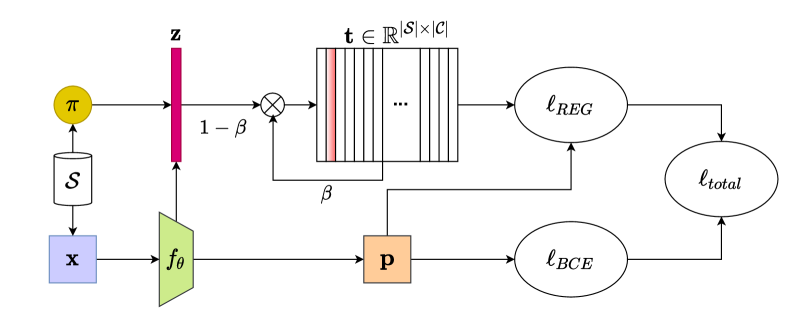
To address the noisy multi-label imbalanced learning problems present in real-world MIA datasets, we introduce the Non-volatile Unbiased Memory (NVUM) training module, which is described in Fig. 1. Our contributions are:
-
•
NVUM that stores a non-volatile running average of model logits to explore the multi-label noise robustness of the early learning stages. This memory module is used by a new regularisation loss to penalise differences between current and early-learning model logits;
-
•
The NVUM update takes into account the class prior distribution to unbias the classification predictions estimated from the imbalanced training set;
- •
2 Method
We assume the availability of a noisy-labelled training set , where is the input image of size with colour channels, and is the noisy label with the set of classes denoted by (note that represents a binary vector in multi-label problems, with each label representing one disease).
2.1 Non-volatile Unbiased Memory (NVUM) Training
To describe the NVUM training, we first need to define the model, parameterised by and represetned as a deep neural network, with , where , denotes the sigmoid activation function and , with representing a logit. The training of the model is achieved by minimising the following loss function:
| (1) |
where denotes the binary cross-entropy loss for handling multi-label classification and is a regularization term defined by:
| (2) |
here is our proposed memory module designed to store an unbiased multi-label running average of the predicted logits for all training samples and uses the class prior distribution for updating, denoted by for . The memory module is initialised with zeros, as in , and is updated in every epoch with:
| (3) |
where is a hyper-parameter controlling the volatility of the memory storage, with set to larger value representing a non-volatile memory and denoting a volatile memory that is used in [7] for contrastive learning.
To explore the early learning phenomenon, we set so the regularization can enforce the consistency between the current model logits and the logits produced at the beginning of the training, when the model is robust to noisy label.
Furthermore, to make the training robust to imbalanced problems, we subtract the log prior of the class distributions, which has the effect of increasing the logits with larger values for the classes with smaller prior.
This counterbalances the issue faced by imbalanced learning problems, where
the logits for the majority classes can overwhelm those from the minority classes, to the point that logit inconsistencies found by the regularization from noisy labels of the majority classes may become indistinguishable from the clean labels from minority classes.
The effect of Eq. (2) can be interpreted by inspecting the loss gradient, which is proved in the supplementary material. The gradient of (1) is:
| (4) |
where is the Jacobian matrix w.r.t. for the sample. Assume is the hidden true label of the sample , then the entry if , and if at the early stages of training. During training, we consider four conditions explained below, where we assume that . When the training sample has clean label:
-
•
if , the gradient of the BCE term, given that the model is likely to fit clean samples. With , the sign of is negative, and the model keeps training for these positive labels even after the early-training stages.
-
•
if , the gradient of the BCE term, given that the model is likely to fit clean samples. Given that , we have , and the model keeps training for these negative labels even after the early-training stages.
Therefore, adding in total loss ensures that clean samples gradient magnitudes remains relatively high, encouraging a continuing optimisation using the clean label samples. For a noisy-label sample, we have:
-
•
if and , the gradient of the BCE loss is because the model will not fit noisy label during early training stages. With , we have , which reduces the gradient magnitude from the BCE loss.
-
•
if and , . Given that , we have , which also reduces the gradient magnitude from the BCE loss.
Therefore, for noisy-label samples, will counter balance the gradient from the BCE loss and diminish the effect of noisy-labelled samples in the training.
3 Experiment
Datasets. For the experiments below, we use the NIH Chest X-ray14 [30] and CheXpert [10] as noisy multi-label imbalanced datasets for training and Indiana OpenI [4] and PadChest [1] datasets for clean multi-label testing sets.
For the noisy sets, NIH Chest X-ray14 (NIH) contains 112,120 CXR images from 30,805 patients. There are 14 labels (each label is a disease), where each patient can have multiple diseases, forming a multi-label classification problem. For a fair comparison with previous papers [8, 26], we adopt the official train/test data split [30]. CheXpert (CXP) contains 220k images with 14 different diseases, and similarly to NIH, each patient can have multiple diseases. For pre-processing, we remove all lateral view images and treat uncertain and empty labels as negative labels. Given that the clean test set from CXP is not available and the clean validation set is too small for a fair comparison, we further split the training images into 90% training set and 10% noisy validation set with no patient overlapping. For the clean sets, Indiana OpenI (OPI) contains 7,470 frontal/lateral images with manual annotations. In our experiments, we only use 3,643 frontal view of images for evaluation. PadChest (PDC) is a large-scale dataset containing 158,626 images with 37.5% of images manually labelled. In our experiment, we only use the manually labelled samples as the clean test set. To keep the number of classes consistent between different datasets, we trim the training and testing sets based on the shared classes between these datasets 222We include a detailed description based on [3] in the supplementary material..
Implementation Details. We use the ImageNet [27] pre-trained DenseNet121 [9] as the backbone model for on NIH and CXP. We use Adam [13] optimizer with batch size 16 for NIH and 64 for CXP. For NIH, we train for 30 epochs with a learning rate of 0.05 and decay with 0.1 at 70% and 90% of the total of training epochs. Images are resized from 10241024 to 512512 pixels. For data augmentation, we employ random resized crop and random horizontal flipping. For CXP, we train for 40 epochs with a learning rate of and follow the learning rate decay policy as on NIH. Images are resized to 224224. For data augmentation, we employ random resized crop, 10 degree random rotation and random horizontal flipping. For both datasets, we use and normalized by ImageNet mean and standard deviation.
All classification results are reported using area under the ROC curve (AUC). To report performance on clean test sets OPI and PDC, we adopt a common noisy label setup [14, 6] that selects the best performance checkpoint on noisy validation, which is the noisy test set of NIH and the noisy validation set of CXP. All experiments are implemented with Pytorch [24] and conducted on an NVIDIA RTX 2080ti GPU. The training takes 15 hours on NIH and 14 hours on CXP.
| Models | ChestXNet [26] | Hermoza et al. [8] | Ma et al. [18] | DivideMix [14] | Ours | |||||
|---|---|---|---|---|---|---|---|---|---|---|
| Datasets | OPI | PDC | OPI | PDC | OPI | PDC | OPI | PDC | OPI | PDC |
| Atelectasis | 86.97 | 84.99 | 86.85 | 83.59 | 84.83 | 79.88 | 70.98 | 73.48 | 88.16 | 85.66 |
| Cardiomegaly | 89.89 | 92.50 | 89.49 | 91.25 | 90.87 | 91.72 | 74.74 | 81.63 | 92.57 | 92.94 |
| Effusion | 94.38 | 96.38 | 95.05 | 96.27 | 94.37 | 96.29 | 84.49 | 97.75 | 95.64 | 96.56 |
| Infiltration | 76.72 | 70.18 | 77.48 | 64.61 | 71.88 | 73.78 | 84.03 | 81.61 | 72.48 | 72.51 |
| Mass | 53.65 | 75.21 | 95.72 | 86.93 | 87.47 | 85.81 | 71.31 | 77.41 | 97.06 | 85.93 |
| Nodule | 86.34 | 75.39 | 82.68 | 75.99 | 69.71 | 68.14 | 57.45 | 63.89 | 88.79 | 75.56 |
| Pneumonia | 91.44 | 76.20 | 88.15 | 75.73 | 84.79 | 76.49 | 64.65 | 72.32 | 90.90 | 82.22 |
| Pneumothorax | 80.48 | 79.63 | 75.34 | 74.55 | 82.21 | 79.73 | 71.56 | 75.46 | 85.78 | 79.50 |
| Edema | 83.73 | 98.07 | 85.31 | 97.78 | 82.75 | 96.41 | 80.71 | 91.81 | 86.56 | 95.70 |
| Emphysema | 82.37 | 79.10 | 83.26 | 79.81 | 79.38 | 75.11 | 54.81 | 59.91 | 83.70 | 79.38 |
| Fibrosis | 90.53 | 96.13 | 86.26 | 96.46 | 83.17 | 93.20 | 76.98 | 84.71 | 91.67 | 98.40 |
| Pleural Thickening | 81.58 | 72.29 | 77.99 | 69.95 | 77.59 | 67.87 | 63.98 | 58.25 | 84.82 | 74.80 |
| Hernia | 89.82 | 86.72 | 93.90 | 89.29 | 87.37 | 86.87 | 66.34 | 72.11 | 94.28 | 93.02 |
| Mean AUC | 83.69 | 83.29 | 86.01 | 83.25 | 82.80 | 82.41 | 70.92 | 76.18 | 88.65 | 85.55 |
3.1 Experiments and Results
Baselines. We compared NVUM with several methods, including the CheXNet baseline [26], Ma et al.’s approach [18] based on a cross-attention network, the current SOTA for NIH on the official test set is the model by Hermoza et al. [8] that is a weakly supervised disease classifier that combines region proposal and saliency detection. We also show results from DivideMix [14], which uses a noisy-label learning algorithm based on small loss sample selection and semi-supervised learning. DivideMix has the SOTA results in many noisy-label learning benchmarks. All methods are implemented using the same DenseNet121 [9] backbone.
Quantitative Comparison Table 1 shows the class-level AUC result for training on NIH and testing on OPI and PDC. Our approach achieves the SOTA results on both clean test sets, consistently outperforming the baselines [26, 8, 18], achieving 2% mean AUC improvement on both test sets. Compared with the current SOTA noisy-label learning DivideMix [14], our method outperforms it by 18% on OPI and 9% on PDC. This shows that for noisy multi-label imbalanced MIA datasets, noisy multi-class balanced approaches based on small-loss selection is insufficient because they do not take into account the multi-label and imbalanced characteristics of the datasets. Table 2 shows class-level AUC results for training on CXP and testing on OPI and PDC. Similarly to the NIH results on Table 1, our approach achieves the best AUC results on both test sets with at least 3% improvement on OPI and 3% on PDC. In addition, DivideMix [14] shows similar results compared with NIH. Hence, SOTA performance on both noisy training sets suggests that our method is robust to different noisy multi-label imbalanced training sets.
| Methods | CheXNet [26] | Hermoza et al. [8] | Ma et al. [18] | DivideMix[14] | Ours | |||||
|---|---|---|---|---|---|---|---|---|---|---|
| Datasets | OPI | PDC | OPI | PDC | OPI | PDC | OPI | PDC | OPI | PDC |
| Cardiomegaly | 84.00 | 80.00 | 87.01 | 87.20 | 82.83 | 85.89 | 71.14 | 66.51 | 88.86 | 88.48 |
| Edema | 88.16 | 98.80 | 87.92 | 98.72 | 86.46 | 97.47 | 75.36 | 95.51 | 88.63 | 99.60 |
| Pneumonia | 65.82 | 58.96 | 65.56 | 53.42 | 61.88 | 54.83 | 57.65 | 40.53 | 64.90 | 67.89 |
| Atelectasis | 77.70 | 72.23 | 78.40 | 75.33 | 80.13 | 72.87 | 73.65 | 64.12 | 80.81 | 75.03 |
| Pneumothorax | 77.35 | 84.75 | 62.09 | 78.65 | 51.08 | 71.57 | 68.75 | 54.05 | 82.18 | 83.32 |
| Effusion | 85.81 | 91.84 | 87.00 | 93.44 | 88.43 | 92.92 | 78.60 | 79.89 | 83.54 | 89.74 |
| Fracture | 57.64 | 60.26 | 57.47 | 53.77 | 59.92 | 60.44 | 60.35 | 59.43 | 57.02 | 62.67 |
| Mean AUC | 76.64 | 78.12 | 75.06 | 77.29 | 72.96 | 76.57 | 69.36 | 65.72 | 77.99 | 80.96 |
OPI
PDC
✓
82.910.78
82.271.02
✓
✓
85.800.04
84.350.35
✓
✓
85.240.70
84.390.21
✓
✓
✓
85.360.11
83.040.79
✓
✓
✓
✓
86.680.16
85.020.18
NVUM
88.170.48
85.490.06
Additional benchmark. Using the recently proposed noisy label benchmark by Xue et al. [32], we further test our approach against the SOTA in the field. The benchmark uses a subset of the official NIH test set [19], with 1,962 CXR images manually re-labelled by at least three radiologists per image. For the results, we follow [32] and consider the AUC results only for Pneumothorax (Pneu) and average of Mass and Nodule (M/N). We use the same hyperparameters as above. The results in Tab. 3 shows that our method outperforms most noisy label methods and achieves comparable performance to [32] on Pneumothorax (88.9 vs 89.1) and better performance on Mass/Nodule (85.5 vs 84.6). However, it is important to mention that differently from [32] that uses two models, we use only one model, so our method requires significantly less training time and computation resources. Furthermore, the clean test set from [19] is much smaller than OPI and PDC with only two classes available, so we consider results in Tab. 1 and 2 more reliable than Tab. 3
3.2 Ablation Study
Different components of NVUM with . We first study in Fig. 2 (left) how results are affected by the prior added on different components of NVUM.
We run each experiment three times and show mean and standard deviation of AUC results.
By adding the class prior to [21], we replace the BCE term in (1) with . We can also add the class prior to
by replacing the regularization term in (1) with .
We observe a 2% improvement for OPI and PDC for both modifications compared to baseline, demonstrating that it is important to handle imbalanced learning in MIA problems. Furthermore, we combine two modifications together and achieve additional 1% improvement. However, instead of directly working on the loss functions, as suggested in [21], we work on the memory module given that it also enforces the early learning phenomenon, addressing the combined noisy multi-label imbalanced learning problem.
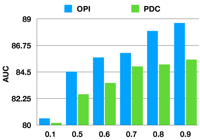
Different . We also study different values for in (3). First, we test a volatile memory update with , which shows a significantly worse performance because the model is overfitting the noisy multi-label of the training set. This indicates traditional volatile memory [7] cannot handle noisy label learning.
Second, the non-volatile memory update with shows a performance that improves consistently with larger . Hence, we use as our default setup.
4 Conclusions and Future Work
In this work, we argue that the MIA problem is a problem of noisy multi-label and imbalanced learning. We presented the Non-volatile Unbiased Memory (NVUM) training module, which stores a non-volatile running average of model logits to make the learning robust to noisy multi-label datasets. Furthermore, The NVUM takes into account the class prior distribution when updating the memory module to make the learning robust to imbalanced learning. We conducted experiments on proposed new benchmark and recent benchmark [32] and achieved SOTA results. Ablation study shows the importance of carefully accounting for imbalanced and noisy multi-label learning. For the future work, we will explore an precise estimation of class prior during the training for accurate unbiasing.
References
- [1] Bustos, A., Pertusa, A., Salinas, J.M., de la Iglesia-Vayá, M.: Padchest: A large chest x-ray image dataset with multi-label annotated reports. Medical image analysis 66, 101797 (2020)
- [2] Cao, K., Wei, C., Gaidon, A., Arechiga, N., Ma, T.: Learning imbalanced datasets with label-distribution-aware margin loss. In: Advances in Neural Information Processing Systems. pp. 1567–1578 (2019)
- [3] Cohen, J.P., Viviano, J.D., Bertin, P., Morrison, P., Torabian, P., Guarrera, M., Lungren, M.P., Chaudhari, A., Brooks, R., Hashir, M., Bertrand, H.: TorchXRayVision: A library of chest X-ray datasets and models. https://github.com/mlmed/torchxrayvision (2020), https://github.com/mlmed/torchxrayvision
- [4] Demner-Fushman, D., Kohli, M.D., Rosenman, M.B., Shooshan, S.E., Rodriguez, L., Antani, S., Thoma, G.R., McDonald, C.J.: Preparing a collection of radiology examinations for distribution and retrieval. Journal of the American Medical Informatics Association 23(2), 304–310 (2016)
- [5] Goldberger, J., Ben-Reuven, E.: Training deep neural-networks using a noise adaptation layer (2016)
- [6] Han, B., Yao, Q., Yu, X., Niu, G., Xu, M., Hu, W., Tsang, I., Sugiyama, M.: Co-teaching: Robust training of deep neural networks with extremely noisy labels. Advances in neural information processing systems 31 (2018)
- [7] He, K., Fan, H., Wu, Y., Xie, S., Girshick, R.: Momentum contrast for unsupervised visual representation learning. arXiv preprint arXiv:1911.05722 (2019)
- [8] Hermoza, R., et al.: Region proposals for saliency map refinement for weakly-supervised disease localisation and classification. arXiv preprint arXiv:2005.10550 (2020)
- [9] Huang, G., et al.: Densely connected convolutional networks. In: CVPR. pp. 4700–4708 (2017)
- [10] Irvin, J., Rajpurkar, P., Ko, M., Yu, Y., Ciurea-Ilcus, S., Chute, C., Marklund, H., Haghgoo, B., Ball, R., Shpanskaya, K., et al.: Chexpert: A large chest radiograph dataset with uncertainty labels and expert comparison. In: Proceedings of the AAAI conference on artificial intelligence. vol. 33, pp. 590–597 (2019)
- [11] Jiang, L., Zhou, Z., Leung, T., Li, L.J., Fei-Fei, L.: Mentornet: Learning data-driven curriculum for very deep neural networks on corrupted labels. In: ICML (2018)
- [12] Kang, B., Xie, S., Rohrbach, M., Yan, Z., Gordo, A., Feng, J., Kalantidis, Y.: Decoupling representation and classifier for long-tailed recognition. arXiv preprint arXiv:1910.09217 (2019)
- [13] Kingma, D.P., Ba, J.: Adam: A method for stochastic optimization. arXiv preprint arXiv:1412.6980 (2014)
- [14] Li, J., Socher, R., Hoi, S.C.: Dividemix: Learning with noisy labels as semi-supervised learning. arXiv preprint arXiv:2002.07394 (2020)
- [15] Litjens, G., Kooi, T., Bejnordi, B.E., Setio, A.A.A., Ciompi, F., Ghafoorian, M., Van Der Laak, J.A., Van Ginneken, B., Sánchez, C.I.: A survey on deep learning in medical image analysis. Medical image analysis 42, 60–88 (2017)
- [16] Liu, F., Tian, Y., Chen, Y., Liu, Y., Belagiannis, V., Carneiro, G.: Acpl: Anti-curriculum pseudo-labelling forsemi-supervised medical image classification. arXiv preprint arXiv:2111.12918 (2021)
- [17] Liu, S., Niles-Weed, J., Razavian, N., Fernandez-Granda, C.: Early-learning regularization prevents memorization of noisy labels. arXiv preprint arXiv:2007.00151 (2020)
- [18] Ma, C., et al.: Multi-label thoracic disease image classification with cross-attention networks. In: MICCAI. pp. 730–738. Springer (2019)
- [19] Majkowska, A., Mittal, S., Steiner, D.F., Reicher, J.J., McKinney, S.M., Duggan, G.E., Eswaran, K., Cameron Chen, P.H., Liu, Y., Kalidindi, S.R., et al.: Chest radiograph interpretation with deep learning models: assessment with radiologist-adjudicated reference standards and population-adjusted evaluation. Radiology 294(2), 421–431 (2020)
- [20] Malach, E., Shalev-Shwartz, S.: Decoupling” when to update” from” how to update”. Advances in Neural Information Processing Systems 30 (2017)
- [21] Menon, A.K., Jayasumana, S., Rawat, A.S., Jain, H., Veit, A., Kumar, S.: Long-tail learning via logit adjustment. arXiv preprint arXiv:2007.07314 (2020)
- [22] Oakden-Rayner, L.: Exploring the chestxray14 dataset: problems. Wordpress: Luke Oakden Rayner (2017)
- [23] Oakden-Rayner, L.: Exploring large-scale public medical image datasets. Academic radiology 27(1), 106–112 (2020)
- [24] Paszke, A., Gross, S., Massa, F., Lerer, A., Bradbury, J., Chanan, G., Killeen, T., Lin, Z., Gimelshein, N., Antiga, L., et al.: Pytorch: An imperative style, high-performance deep learning library. Advances in neural information processing systems 32 (2019)
- [25] Patrini, G., Rozza, A., Krishna Menon, A., Nock, R., Qu, L.: Making deep neural networks robust to label noise: A loss correction approach. In: Proceedings of the IEEE conference on computer vision and pattern recognition. pp. 1944–1952 (2017)
- [26] Rajpurkar, P., et al.: Chexnet: Radiologist-level pneumonia detection on chest x-rays with deep learning. arXiv preprint arXiv:1711.05225 (2017)
- [27] Russakovsky, O., et al.: Imagenet large scale visual recognition challenge. IJCV 115(3), 211–252 (2015)
- [28] Tan, J., Wang, C., Li, B., Li, Q., Ouyang, W., Yin, C., Yan, J.: Equalization loss for long-tailed object recognition. In: Proceedings of the IEEE/CVF conference on computer vision and pattern recognition. pp. 11662–11671 (2020)
- [29] Tang, K., Huang, J., Zhang, H.: Long-tailed classification by keeping the good and removing the bad momentum causal effect. In: NeurIPS (2020)
- [30] Wang, X., Peng, Y., Lu, L., Lu, Z., Bagheri, M., Summers, R.M.: Chestx-ray8: Hospital-scale chest x-ray database and benchmarks on weakly-supervised classification and localization of common thorax diseases. In: CVPR. pp. 2097–2106 (2017)
- [31] Xia, X., Liu, T., Wang, N., Han, B., Gong, C., Niu, G., Sugiyama, M.: Are anchor points really indispensable in label-noise learning? arXiv preprint arXiv:1906.00189 (2019)
- [32] Xue, C., Yu, L., Chen, P., Dou, Q., Heng, P.A.: Robust medical image classification from noisy labeled data with global and local representation guided co-training. IEEE Transactions on Medical Imaging (2022)
- [33] Zhang, Z., Li, Y., Wei, H., Ma, K., Xu, T., Zheng, Y.: Alleviating noisy-label effects in image classification via probability transition matrix. arXiv preprint arXiv:2110.08866 (2021)
5 Appendix: Gradient Proof
The gradient for is defined as
| (5) |
where , and recalling that (with ), we have
| (6) |
6 Appendix: Dataset Description
| Training Scheme | NIH/CXP | OPI | PDC | Number of Classes |
|---|---|---|---|---|
| NIH-OPI-PDC | 83,672 | 2,971 | 14,714 | 14 |
| CXP-OPI-PDC | 170,958 | 2,823 | 12,885 | 8 |
7 Appendix: Synthetic Label Noise Result
We include results using the public noisy-label medical image benchmark from [33] to test our method for different rates of symmetric noise. We tested our method on their ResNet-18 benchmark, where their baseline accuracy result using the 100% clean set is 64.4%. With 20% symmetric noise, our method without our prior reaches 61.3% and with our prior has 63.1% (best result in [33]: 59.37%). With 40% symmetric noise, our method without our prior reaches 50.7% and with our prior has 53.4% (best result in [33]: 49.65%).
8 Appendix: Memory Footprint
We analysis the memory footprint of our method. In particular, our memory module is a matrix with N x C dimension. We used debugging tools to analyse our memory module and noted that we only required 4 MB of GPU memory, and at each iteration, we only backpropagated through a small subset of the memory.