Metallicity dependence of the H/H₂ and C⁺/C/CO distributions in a resolved self-regulating interstellar medium

Abstract

We study the metallicity dependence of the H/H₂ and C⁺/C/CO distributions in a self-regulated interstellar medium (ISM) across a broad range of metallicities ($0.1<Z/Z_{\odot}<3$). To this end, we conduct high-resolution (particle mass of $1\ {\rm M_{\odot}}$) hydrodynamical simulations coupled with a time-dependent H₂ chemistry network. The results are then post-processed with an accurate chemistry network to model the associated C⁺/C/CO abundances, based on the time-dependent non-steady-state (“non-equilibrium”) H₂ abundances. We find that the time-averaged star formation rate and the ISM structure are insensitive to metallicity. The column densities relevant for molecular shielding appear correlated with the volume densities in gravitationally unstable gas. As metallicity decreases, H₂ progressively deviates from steady state (“equilibrium”) and shows shallow abundance profiles until they sharply truncate at the photodissociation fronts. In contrast, the CO profile is sharp and controlled by photodissociation as CO quickly reaches steady state. We construct effective one-dimensional cloud models that successfully capture the time-averaged chemical distributions in simulations. At low metallicities, the steady-state model significantly overestimates the abundance of H₂ in the diffuse medium. The overestimated H₂, however, has little impact on CO. Consequently, the mass fraction of CO-dark H₂ gas is significantly lower than what a fully steady-state model predicts. The mass ratios of H₂/C⁺ and H₂/C both show a weaker dependence on $Z^{\prime}$ than H₂/CO, which potentially indicates that C⁺ and C could be alternative tracers for H₂ at low $Z^{\prime}$ in terms of mass budget. Our chemistry code for post-processing is publicly available.

1 Introduction

Stars are formed in molecular hydrogen (H₂) gas, as ubiquitously observed in our Milky Way (Lada & Lada, 2003; Evans et al., 2009), in nearby galaxies (Bigiel et al., 2008; Leroy et al., 2008), and all the way to high-redshift galaxies (Genzel et al., 2010; Tacconi et al., 2020). H₂ does not radiate efficiently at the typical temperatures of molecular clouds and thus is not directly visible. As such, carbon monoxide (CO), which is an efficient line emitter and whose formation relies on the presence of H₂, is routinely used as an observable tracer for H₂ (Bolatto et al., 2013).

However, CO emission becomes very faint and is often non-detectable at low metallicities (Leroy et al., 2005; Schruba et al., 2012; Cormier et al., 2014; Hunt et al., 2015). This is expected as the CO formation rates are reduced and the low dust abundance provides less shielding against the far-ultraviolent (FUV) radiation. CO is thus further photodissociated into the clouds, leading to a potentially large “CO-dark” H₂ reservoir in low-metallicity galaxies (Madden et al., 1997; Pak et al., 1998; Bolatto et al., 1999; Wolfire et al., 2010; Bolatto et al., 2013). Therefore, alternative tracers for H₂ have been proposed such as ionized carbon C⁺ (Madden et al., 1997; De Looze et al., 2011; Zanella et al., 2018; Dessauges-Zavadsky et al., 2020; Madden et al., 2020) and atomic carbon C (Papadopoulos et al., 2004; Walter et al., 2011; Andreani et al., 2018; Jiao et al., 2019; Bourne et al., 2019; Valentino et al., 2020), though their feasibility and robustness require further investigations. Therefore, understanding the distributions of C⁺/C/CO in different environments is a crucial step to assess the pros and cons of these different tracers.

However, such theoretical considerations adopt a static view of the interstellar medium (ISM), which is highly dynamic in reality. Gas radiatively cools, gravitationally collapses and forms stars, which in turn inject energy and momentum back to the ISM via stellar feedback, heating up the gas, driving turbulence and destroying clouds. This cycle occurs rapidly and thus a realistic picture of the ISM must include these dynamical effects.

Substantial efforts have been made using hydrodynamical simulations to study the chemical properties of the dynamic ISM over the past decade. Glover & Mac Low (2011) and Glover & Clark (2012a) conducted simulations of turbulent clouds to study the relationship between H₂ and CO and quantify the CO-to-H₂ conversion factor, $X_{\rm CO}$, as a function of visual extinction and metallicity. Cloud simulations, however, are limited by their unrealistic initial and boundary conditions as well as their artificial driving force, rendering them incapable of following the formation and destruction of clouds self-consistently. On the other hand, the metallicity dependence of $X_{\rm CO}$ has also been investigated by Narayanan et al. (2012) in galaxy mergers and Feldmann et al. (2012) in cosmological simulations, respectively. As these studies focus on a much larger scale, their spatial resolution is rather limited ($\sim 70$ pc), preventing them from resolving the multi-phase ISM structure and stellar feedback that require at least pc-scale resolution. Consequently, highly uncertain sub-resolution models have to be adopted, diminishing their predictive power. Simulations of an isolated Milky Way-type galaxy (Duarte-Cabral et al., 2015; Richings & Schaye, 2016) allow for a somewhat better resolution, but still far from what is required and thus face similar issues.

More recently, the SILCC simulations (Walch et al., 2015; Girichidis et al., 2016; Seifried et al., 2017) used the “stratified box” setup to study a patch of the ISM regulated by stellar feedback for solar-neighborhood conditions, featuring a time-dependent chemistry network from Glover & Mac Low (2007) and Glover & Clark (2012b). The TIGRESS simulations (Kim & Ostriker, 2017; Kim et al., 2020) adopted a similar setup but without the time-dependent chemistry. Instead, their results were later post-processed by Gong et al. (2018) with their improved chemistry network (Gong et al., 2017) to obtain steady-state chemical abundances. Using the same chemistry as SILCC, “The Cloud Factory” (Smith et al., 2020) simulated a much larger patch of the Galaxy and with a mesh refinement technique to follow the formation of clouds down to a remarkable mass resolution of 0.25 ${\rm M_{\odot}}$ albeit only for a short amount of time (4 Myr).

Another promising approach is to simulate an isolated dwarf galaxy that is small enough to achieve the necessary resolution. Hu et al. (2016) and Hu et al. (2017) studied a dwarf galaxy with $Z^{\prime}\equiv Z/Z_{\odot}=0.1$ using the same chemistry as SILCC and found very little H₂ in the ISM, concluding that the star formation reservoir is dominated by the atomic gas. On the other hand, using the Grackle chemistry network (Smith et al., 2017), Emerick et al. (2019) simulated an even smaller galaxy with the same metallicity but found a significantly larger H₂ fraction.

All of these resolved ISM simulations, however, have been focused only on a particular metallicity. A systematic investigation across a broad range of metallicities in the framework of a self-regulated ISM is therefore urgently needed. Very recently, Gong et al. (2020) post-processed the results of Kim et al. (2020) and studied the systematic variations of several physical parameters including metallicity in the range of $0.5<Z^{\prime}<2$. However, their simulations were all run with $Z^{\prime}=1$ which is inconsistent with the post-processed chemistry. More importantly, by post-processing, they were forced to assume steady-state chemistry which, as we will demonstrate, significantly over-produces H₂ (but not CO), especially at low metallicities.

While the chemistry network for H₂ is relatively small and can be efficiently coupled with simulations, the network involving CO is significantly larger (Dalgarno & Black, 1976; van Dishoeck & Black, 1988; Sternberg & Dalgarno, 1995). Therefore, coupling the full CO network with simulations implies a formidable computational overhead, which motivated efforts to trim down the network to a minimum level. In a comparison study, Glover & Clark (2012b) showed that the simplest and most widely used network of Nelson & Langer (1997) (NL97), while computationally efficient, tends to over-produce CO. In contrast, the network of Nelson & Langer (1999) (NL99) is able to reproduce accurate results comparable to the much more comprehensive network of Glover et al. (2010). In practice, however, even the NL99 network is already a nontrivial computational overhead and therefore is rarely applied to ISM simulations.

In this work, we study the metallicity dependence of the H/H₂ and C⁺/C/CO distributions in a stellar feedback-regulated ISM across a broad range of metallicities $0.1<Z^{\prime}<3$. We conduct stratified-box simulations which self-consistently include a time-dependent H₂ chemistry and cooling, star formation with individual stars, and feedback from photoionization and supernovae (SNe). To obtain the abundances of C⁺, C and CO, we post-process our simulations with a detailed chemistry network that includes 31 species and 286 reactions, taking the time-dependent H₂ abundance into account. With this hybrid technique, we are able to achieve a very high resolution (particle mass of $1\ {\rm M_{\odot}}$, spatial resolution $\sim$ 0.2 pc), capture the time-dependent nature of H₂ formation in a dynamical ISM, and accurately model CO with all its major formation and destruction channels simultaneously.

This paper is organized as follows. In Sec. 2, we describe our numerical method and the setup of our simulations. In Sec. 3, we introduce the more detailed chemistry network that we use to post-process the chemical species. In Sec. 4, we present our simulation results, focusing on the metallicity dependence of the ISM structure and the chemical compositions. In Sec. 5, we compare our results with previous studies and discuss the potential caveats. In Sec. 6, we summarize our paper.

2 Simulation method

2.1 Gravity and hydrodynamics

We use the public version of Gizmo (Hopkins, 2015), a multi-solver code featuring the meshless Godunov method (Gaburov & Nitadori, 2011) on top of the TreeSPH code Gadget-3 (Springel, 2005). The gravitational interaction is solved by the Barnes–Hut algorithm (“treecode”) while hydrodynamics is solved by the meshless finite-mass (MFM) method (Hopkins, 2015) with the number of neighboring particles in a kernel $N_{\rm ngb}=32$.

2.2 Cooling, heating and chemistry

We use a time-dependent hydrogen chemistry network developed in Glover & Mac Low (2007) and Glover & Clark (2012b), which has been applied extensively in previous ISM simulations coupled with several different codes (e.g., Smith et al., 2014; Walch et al., 2015; Girichidis et al., 2016; Hu et al., 2016, 2017; Gatto et al., 2017; Smith et al., 2020). The network includes H₂ formation on dust, H₂ destruction by photodissociation, collisional dissociation and cosmic ray ionization, and recombination in the gas phase and on dust grains. Cooling processes include fine structure metal lines, molecular lines, Lyman alpha, H₂ collisional dissociation, collisional ionization of H, and recombination of H⁺ in the gas phase and on grains. Heating processes include photoelectric emission from dust, cosmic ray ionization, H₂ photodissociation, UV pumping of H₂ and the formation of H₂.

The cosmic ray ionization rate of H₂ ($\zeta_{\rm CR}$) and the energy density of the unattenuated FUV radiation field ($u_{\rm UV}$) are both spatially constant but time-dependent, linearly scaled with the star formation rate (SFR) surface density $\Sigma_{\rm SFR}$ projected face-on (see Sec. 2.6), i.e., $\zeta_{\rm CR}=(\Sigma_{\rm SFR}/\Sigma_{\rm SFR,0})\zeta_{\rm CR,0}$, where we use the local values for normalization: $\zeta_{\rm CR,0}=10^{-16}\ {\rm s^{-1}}$ (Indriolo & McCall, 2012; Indriolo et al., 2015) and $\Sigma_{\rm SFR,0}=2.4\times 10^{-3}\ {\rm M_{\odot}\ yr^{-1}\ kpc^{-2}}$ (Fuchs et al., 2009). Similarly, $u_{\rm UV}=I_{\rm UV}u_{\rm UV,0}$ where $u_{\rm UV,0}=8.94\times 10^{-14}\ {\rm erg\ cm^{-3}}$ is the Draine field (Draine, 1978) and $I_{\rm UV}\equiv\max(\Sigma_{\rm SFR}/\Sigma_{\rm SFR,0},I_{\rm UV,min})$. The floor $I_{\rm UV,min}=0.002$ accounts for the cosmic UV background (Haardt & Madau, 2012). We define the SFR as the total mass of stars younger than $t_{\rm SFR}$ divided by $t_{\rm SFR}$, and we adopt $t_{\rm SFR}=30$ Myr motivated by the lifetime of an ${\rm 8M_{\odot}}$-star.

Both dust and H₂ self-shielding against FUV radiation are accounted for by a method similar to Clark et al. (2012). The HealPix algorithm (Górski & Hivon, 2011) is used to define 12 different pixels centered at each gas particle. Along each pixel, we calculate the column densities of gas up to a pre-defined shielding length $L_{\rm sh}$. The tree structure for gravity is used to speed up the calculation. A treenode is assigned to a pixel if its center of mass is located within the pixel. We choose $L_{\rm sh}=100$ pc motivated by the typical separation between OB associations in the solar neighborhood (Parravano et al., 2003; Bialy, 2020). The choice of $L_{\rm sh}$ only has a minor effect on the total molecular masses and is explored in Appendix B.1.

2.3 Star formation

We adopt a stochastic star formation recipe commonly used in the field of galaxy formation. Star formation occurs when the local velocity divergence becomes negative (i.e., converging flows) and the thermal Jeans mass of gas $M_{\rm J}=(\pi^{2.5}c_{s}^{3})/(6G^{1.5}\rho^{0.5})$ drops below the kernel mass $M_{\rm ker}=N_{\rm ngb}m_{\rm g}$, where $c_{s}$ is the sound speed, $G$ is the gravitational constant, $\rho$ is the gas density and $m_{\rm g}$ is the gas particle mass. Equivalently, this corresponds to the requirement

$$n>1.26\times 10^{4}{\rm cm^{-3}}\Big{(}\frac{T}{30{\rm K}}\Big{)}^{3}\Big{(}\frac{m_{\rm g}}{{\rm M_{\odot}}}\Big{)}^{-2}\Big{(}\frac{\mu}{2.3}\Big{)}^{-3},$$ (1)

where $n=X_{\rm H}\rho/m_{\rm p}$ is the hydrogen number density, $X_{\rm H}=0.71$ is the hydrogen mass fraction, $m_{\rm p}$ is the proton mass, $T$ is the gas temperature and $\mu$ is the mean molecular weight. Each gas particle that fulfills these requirements has a probability of $\epsilon_{\rm sf}\Delta t/t_{\rm ff}$ to be converted into a star particle, where $\Delta t$ is the timestep, $t_{\rm ff}=\sqrt{3\pi/(32G\rho)}$ is the gas free-fall time and $\epsilon_{\rm sf}$ is the star formation efficiency. A gas particle will therefore be converted into a star particle in roughly $t_{\rm ff}/\epsilon_{\rm sf}$. We adopt $\epsilon_{\rm sf}=0.5$ throughout this work as our resolution is capable of resolving the detailed structure of molecular clouds. In addition, we impose a threshold density $n_{\rm isf}=10^{5}\ {\rm cm^{-3}}$ beyond which gas is converted into stars instantaneously, irrespective of the above-mentioned requirements. The effect of $n_{\rm isf}$ is discussed in Appendix C.1. A star particle will inherit the position, velocity and mass of its gas progenitor but will no longer interact hydrodynamically.

2.4 IMF sampling for individual stars

Massive stars (initial mass $>8\ {\rm M_{\odot}}$) inject energy and momentum into their surrounding gas which counters cooling and gravitational collapse, regulating the ISM. In contrast to large-scale cosmological simulations where a star particle is massive enough to represent a star cluster that fully samples the stellar initial mass function (IMF), care must be taken in our case as the mass of star particles ($m_{*}=1{\rm M_{\odot}}$) becomes too low to represent even a massive star. Here we present a simple method designed for high-resolution simulations. In a uniformly sampled IMF, there is on average one massive star in every $M_{\rm IMF}=$ 100 M_⊙ of stellar mass assuming the Kroupa IMF (Kroupa, 2001). Therefore, each star particle has a probability of $m_{*}/M_{\rm IMF}$ for being marked as a massive-star tracer. The stellar mass of the tracer is determined stochastically following an IMF on the high-mass end, which can be realized by the method of importance sampling:

$$m_{\rm star}=[(m_{\rm max}^{\alpha}-m_{\rm min}^{\alpha})y+m_{\rm min}^{\alpha}]^{-1/\alpha}$$ (2)

where $y$ is a random number uniformly distributed between 0 and 1, $\alpha$ is the power-law index on the high-mass end, and $m_{\rm min}=8{\rm M_{\odot}}$ and $m_{\rm max}=50{\rm M_{\odot}}$ are the lower and upper bound for the sampled mass, respectively. We note that $m_{\rm star}$ is insensitive to moderate variation of $m_{\rm max}$ as stars more massive than 50 ${\rm M_{\odot}}$ are very rare (less than 1% of the total massive stars by number). We adopt $\alpha=1.3$ appropriate for the Kroupa IMF. The sampled $m_{\rm star}$ is used to determine the stellar lifetime (Ekström et al., 2012) and luminosity of ionizing radiation from the BaSeL stellar library (Lejeune et al., 1997, 1998), while the gravitational mass of the star particles ($m_{*}$) remains unchanged.

We note that our method of IMF sampling is similar to that presented in Hu et al. (2017) but different in two aspects: (i) we do not modify the gravitational mass and (ii) we do not allow multiple tracers for a single star particle, which only happens when the resolution becomes so coarse that $m_{*}>M_{\rm IMF}$. Our method is easy to implement and remains applicable when one wants to trace individual stellar masses below $8{\rm M_{\odot}}$ (e.g. for the purpose of metal enrichment from the asymptotic giant branch stars) by lowering $m_{\rm min}$ (and adjusting $M_{\rm IMF}$ accordingly).

2.5 Stellar feedback

Massive stars emit hydrogen-ionizing radiation continuously throughout their lifetimes. Our photoionization feedback is based on Hu et al. (2017) which uses an iterative method to define the ionization front within which the gas is heated up to $10^{4}$ K. The balance between recombination and photoionization is evaluated using the density of the photoionized gas which can be different from the gas density around the star. This approach captures the dynamical evolution of a D-type photoionization front in a uniform medium as accurately as radiative transfer methods. Moreover, it can be applied to overlapping HII regions where a naive Strömgren-sphere method would fail.

Massive stars explode as core-collapse SNe by the end of their lifetimes. Our SN feedback is purely thermal, i.e., an SN injects $10^{51}$ erg into its nearest 32 gas particles as thermal energy weighted by the kernel function. As we are working at the resolution where the Sedov-Taylor phase of SN remnant is always well-resolved, the dynamical effect of SN feedback on the ISM is insensitive to the form of energy injection (i.e., kinetic, thermal, or mixed) as shown in Hu (2019).

2.6 Simulation setup

We use the “stratified box” setup which consists of an elongated box representing a patch of a disk galaxy, that, in our case, is a model for the solar neighborhood. The box size is 1 kpc along the $x$- and $y$-axes with periodic boundary conditions and 10 kpc along the $z$-axis with outflow boundary conditions. The origin is defined at the box center and $z=0$ represents the mid-plane of the galaxy such that $z=\pm 5$ kpc are the (open) boundaries. The gas initially follows a vertical (along the $z$-axis) density profile: $\rho(z)=(\Sigma_{\rm g}/(2H_{\rm g})\sech^{2}(z/H_{\rm g})$, where $\Sigma_{\rm g}=10\ {\rm M_{\odot}pc^{-2}}$ is the gas surface density and $H_{\rm g}=0.25$ kpc is the scale-height of the gaseous disk. The resulting vertical gravitational acceleration due to self-gravity is

$$a_{\rm g}=-2\pi G\Sigma_{\rm g}\tanh\Big(\frac{z}{H_{\rm g}}\Big{missing}),$$ (3)

and evolves according to the movement of gas.

We include external gravity from the stellar disk that exerts vertical gravitational acceleration:

$$a_{*}=-2\pi G\Sigma_{*}\tanh\Big(\frac{z}{H_{*}}\Big{missing}),$$ (4)

where $\Sigma_{*}=40\ {\rm M_{\odot}pc^{-2}}$ is the stellar surface density and $H_{*}=$ 0.25 kpc is the scale-height of the stellar disk. In addition, we include vertical gravitational acceleration from a dark matter halo which follows an NFW profile (Navarro et al., 1997) with a virial mass $M_{\rm vir}=10^{12}{\rm M_{\odot}}$ and concentration $c=12$:

$$a_{\rm DM}=-\frac{Gm(r)z}{r^{3}}$$ (5)

where $r=\sqrt{z^{2}+R_{0}^{2}}$ is the spherical radius from the center of the halo, $m(r)=4\pi r_{s}^{3}\rho_{s}\ln[(1+r/r_{s})-(r/r_{s})(1+r/r_{s})]$ is the enclosed mass, $r_{s}=17$ kpc, $\rho_{s}=9.5\times 10^{-3}{\rm M_{\odot}pc^{-3}}$, and $R_{0}=8$ kpc is the galactocentric radius of the Sun.

Our periodic boundary conditions for self-gravity are only pseudo-periodic. Namely, we only account for self-gravity from the nearest 3-by-3 periodic images in the $x$ and $y$ directions. This is a good approximation as the large-scale gravitational potential is dominated by the external stellar disk. Furthermore, mathematically robust periodic boundary conditions are not necessarily a better approximation of a galaxy, which is not infinitely large and has a radial distribution of gas. We have tested and confirmed that our results are largely unchanged even when we include 9-by-9 periodic images.

We adopt a mass resolution of $m_{\rm g}=1\ {\rm M_{\odot}}$ which safely resolves every SN event in our simulations (Hu et al., 2016; Hu, 2019). Given $X_{\rm H}=0.71$ and $N_{\rm ngb}=32$, the radius of the MFM kernel (which corresponds to the spatial resolution) is

$$h=6\ {\rm pc}\Big{(}\frac{n}{{\rm cm^{-3}}}\Big{)}^{-1/3}\Big{(}\frac{m_{\rm g}}{{\rm M_{\odot}}}\Big{)}^{1/3}.$$ (6)

At the typical density where the Jeans mass becomes unresolved and star formation occurs, which turns out to be $n\approx 10^{4}\ {\rm cm^{-3}}$, $h\approx 0.2$ pc. Therefore, the gravitational softening length is chosen to be $\epsilon_{\rm soft}=$ 0.2 pc for both gas and stars.

The gas temperature is initially set to $10^{4}$ K uniformly. The metallicity and dust-to-gas mass ratio (DGR) are both constant throughout the simulations. We define a normalized metallicity $Z^{\prime}=Z/Z_{\odot}$ such that $Z^{\prime}=1$ represents solar metallicity. Similarly, we define a normalized DGR that scales linearly with metallicity such that $Z_{d}^{\prime}=Z^{\prime}$ and $Z_{d}^{\prime}=1$ corresponds a DGR of 1%. The initial gas-phase metal abundances are set to be $x_{\rm C,0}=1.4\times 10^{-4}Z^{\prime}$, $x_{\rm O,0}=3.2\times 10^{-4}Z^{\prime}$ and $x_{\rm Si,0}=1.7\times 10^{-6}Z^{\prime}$ based on Cardelli et al. (1994) and Sembach et al. (2000).

We run a set of four simulations at different metallicities $Z^{\prime}=$ 3, 1, 0.3 and 0.1. Each simulation is run for 600 Myr. In the initial 100 Myr, we artificially set the lifetime of massive stars to zero. This forces SN feedback to occur intermediately after star formation and in dense environments by construction which results in a less violent ISM (Gatto et al., 2015; Walch et al., 2015). We do so in order to circumvent the problematic initial transient phase where the entire disk is first violently blown off by SN feedback and then slowly falls back to the mid-plane. This is a simple alternative method to the initial artificial turbulent driving (Walch et al., 2015; Kim & Ostriker, 2017) or random SN driving (Hu et al., 2017) in the literature. As the first 100 Myr is an artificial phase, there is no need to run it with four different metallicities. To save computational resources, simulations with $Z^{\prime}=$ 3, 0.3 and 0.1 are started from $t=100$ Myr using the snapshot in the $Z^{\prime}=1$ case.

3 Post-processing Chemistry

3.1 Chemistry network

Once the simulations are complete, we apply another much more comprehensive chemistry network in post-processing to calculate the CO abundance for each gas particle. Our network follows 31 species: H, H^-, H₂, H⁺, H${}_{2}^{+}$, H${}_{3}^{+}$, e^-, He, He⁺, HeH⁺, C, C⁺, CO, HCO⁺, O, O⁺, OH, OH⁺, H₂O⁺, H₃O⁺, H₂O, O₂, CO⁺, O${}_{2}^{+}$, CH₂, CH${}_{2}^{+}$, CH, CH⁺, CH${}_{3}^{+}$, Si⁺ and Si. We include all chemical reactions in the UMIST database (McElroy et al., 2013) that exclusively involve the above-mentioned species (including photoreactions, cosmic-ray ionization and cosmic-ray-induced photoreactions), which leads to 286 reactions in total. The rate coefficients are also taken from the UMIST database. As the UMIST database assumes a constant $\zeta_{\rm CR,u}=1.2\times 10^{-17}{\rm s^{-1}}$, we scale the appropriate rate coefficients for all the cosmic-ray processes by a factor of $\zeta_{\rm CR}/\zeta_{\rm CR,u}$ accordingly. As there are five chemical elements involved in our network, we can derive six species from the mass and charge conservations without explicitly solving them. We choose to derive the neutral atomic form of each element and the free electron (i.e., H, He, C, O, Si and e^-).

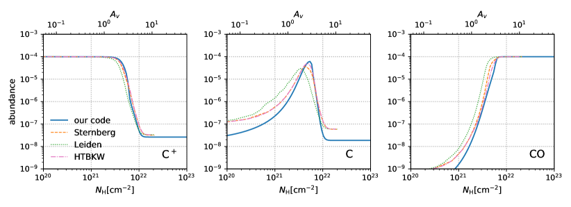
Figure 1: Chemical abundances as a function of $N$ (lower $x$-axis) and $A_{V}$ (upper $x$-axis) for C⁺ (left), C (middle), and CO (right) in a 1D PDR calculation. The solid blue line is from our chemistry network, while the others are from three different codes in the code comparison project (Röllig et al., 2007). The physical parameters are $n=1000\ {\rm cm^{-3}}$, $T=50$ K, $Z^{\prime}=1$, $I_{\rm UV}=10$, and $\zeta_{\rm CR}=10^{-16}{\rm s^{-1}}$ (the “F1” test). Our results agree very well with the others in general, demonstrating that our network can accurately capture the C⁺/C/CO transitions.

In addition to the reactions from the UMIST database, we also include H₂ formation on dust and photodissociation of H₂ and CO by the FUV radiation. Following Hollenbach & McKee (1979) and assuming a dust temperature of 15 K, the rate coefficient of H₂ formation on dust is

$$R_{\rm H_{2}}=\frac{3\times 10^{-17}\sqrt{T_{2}}Z_{d}^{\prime}}{1+0.4\sqrt{T_{2}+0.15}+0.2T_{2}+0.08T_{2}^{2}}\ {\rm cm^{3}s^{-1}},$$ (7)

where $T_{2}\equiv T/(100\ {\rm K})$. The H₂ photodissociation rate coefficient is

$$k_{\rm H_{2}}=I_{\rm UV}k_{\rm 0,H_{2}}f_{\rm dust,H_{2}}f_{\rm ss,H_{2}},$$ (8)

where $k_{\rm 0,H_{2}}$ is the unattenuated rate coefficient for a Draine field, $f_{\rm dust,H_{2}}$ is the dust shielding factor which depends on the visual extinction

$$A_{V}=f_{A_{V}}N,$$ (9)

where $f_{A_{V}}\equiv 5.35\times 10^{-22}Z_{d}^{\prime}$ and $N$ is the total hydrogen column density. $f_{\rm ss,H_{2}}$ is the H₂ self-shielding factor which is a function of H₂ column density $N_{\rm H_{2}}$. Similarly, the CO photodissociation rate coefficient is

$$k_{\rm CO}=I_{\rm UV}k_{\rm 0,CO}f_{\rm dust,CO}f_{\rm gas,CO},$$ (10)

where $k_{\rm 0,CO}$ is the unattenuated rate coefficient, $f_{\rm dust,CO}$ is the dust shielding factor and $f_{\rm gas,CO}$ is the shielding factor from H₂ shielding and CO self-shielding, which is a function of both $N_{\rm H_{2}}$ and $N_{\rm CO}$ (CO column density). Following Heays et al. (2017), we adopt the two-sided slab model where $k_{\rm 0,H_{2}}=5.68\times 10^{-11}\ {\rm s^{-1}}$ (Sternberg et al., 2014), $k_{\rm 0,CO}=2.43\times 10^{-10}\ {\rm s^{-1}}$, $f_{\rm dust,H_{2}}=\alpha_{\rm H_{2}}\exp(-\gamma_{\rm H_{2}}A_{V})$ where $\alpha_{\rm H_{2}}=0.52$ and $\gamma_{\rm H_{2}}=3.85$, and $f_{\rm dust,CO}=\alpha_{\rm CO}\exp(-\gamma_{\rm CO}A_{V})$ where $\alpha_{\rm CO}=0.48$ and $\gamma_{\rm CO}=3.51$. For the self-shielding factors, we follow Draine & Bertoldi (1996) for $f_{\rm ss,H_{2}}$ (assuming an H₂ velocity dispersion of 2 ${\rm km\ s^{-1}}$) and Visser et al. (2009) for $f_{\rm gas,CO}$ (assuming a CO excitation temperature of 5 K and a CO linewidth of 0.3 km s^-1). Recombination on grains (X⁺ + gr $\rightarrow$ X + gr⁺, where X is a chemical element and gr stands for grains) for H, He, C and Si are also included following Weingartner & Draine (2001) (see the discussion in Appendix B.2). We use the solver Differentialequations.jl (Rackauckas & Nie, 2017) to integrate the system of rate equations.

As a validation of our chemistry network, we perform the “F1” test from the code comparison project in Röllig et al. (2007). The test consists of a one-dimensional (1D) calculation of a photon-dominated region (PDR) with $n=1000\ {\rm cm^{-3}}$, $T=50$ K, $Z^{\prime}=1$, $I_{\rm UV}=10$, and $\zeta_{\rm CR}=10^{-16}\ {\rm s^{-1}}$. The initial elemental abundances relative to hydrogen are, respectively, $x_{\rm He,0}=0.1$, $x_{\rm C,0}=1.0\times 10^{-4}$, $x_{\rm O,0}=3.0\times 10^{-4}$, and $x_{\rm Si,0}=0$. Recombination on grains is switched off in order to be consistent with Röllig et al. (2007). Fig. 1 shows the chemical abundances as a function of $N$ (lower $x$-axis) and $A_{V}$ (upper $x$-axis) for C⁺ (left), C (middle), and CO (right). The solid blue line is from our chemistry network, while the others are from three different codes (among many others) participated in Röllig et al. (2007): Sternberg in orange dashed (Sternberg & Dalgarno, 1995; Boger & Sternberg, 2005) Leiden in green dotted (Black & van Dishoeck, 1987; van Dishoeck & Black, 1988), and HTBKW in pink dash-dotted (Tielens & Hollenbach, 1985; Kaufman et al., 1999). Our results agree very well with these codes in general, demonstrating that our network can accurately capture the C⁺/C/CO transitions in a 1D uniform medium.

3.2 Time-dependent vs. steady-state H₂ model

For each simulation snapshot, we run our network for every gas particle up to steady state (run for 1 Gyr), taking the local gas density and temperature as input parameters. The same metallicity and solar abundances ($x_{\rm C,0}=1.4\times 10^{-4}Z^{\prime}$, $x_{\rm O,0}=3.2\times 10^{-4}Z^{\prime}$ and $x_{\rm Si,0}=1.7\times 10^{-6}Z^{\prime}$) are adopted as those in the simulations, as well as the time-dependent $I_{\rm UV}$ and $\zeta_{\rm CR}$ which scales with the current SFR (see Sec. 2.2). However, since $x_{\rm H_{2}}$ and $x_{\rm H^{+}}$ are already calculated from our time-dependent hydrogen network, these two species are used as input parameters. By doing so, we allow H₂ to be out of steady state which happens when the dynamical time controlled by turbulence motions or cloud destruction is shorter than the H₂ formation time

$$t_{\rm H_{2},form}=\frac{1}{2R_{\rm H_{2}}n}\approx 15\ {\rm Myr}\frac{1}{n_{2}Z_{d}^{\prime}},$$ (11)

where $n_{2}\equiv n/({\rm 100\ cm^{-3}})$. All the other species, including C⁺, C and CO, are evolved up to steady state. As shown in Appendix A, the chemical timescales for C⁺, C and CO to reach steady state are short compared to the dynamical time in our simulations, justifying our steady-state assumption. We will refer to these results as our time-dependent H₂ model, which is our default model.

For comparison purposes, we run another set of post-processing without using $x_{\rm H_{2}}$ and $x_{\rm H^{+}}$ from the simulations and obtain steady-state solutions for all species. We will refer to these results as our steady-state H₂ model, which, while less realistic than the time-dependent one, can provide useful insights. Note that the CO abundance can be different in these models despite being in steady state in both cases because (i) CO formation is initiated by H₂ and (ii) H₂ provides shielding for CO.

3.3 Radiation shielding and column densities

Radiation shielding is accounted for using the same HealPix-based method as in the time-dependent network (see Sec. 2.2). Because of self-shielding, local abundances of H₂ and CO depend on those from a distance and therefore a few iterations are required. We find that three iterations are enough to obtain converged results (see Appendix C.3).

We distinguish between the observed total hydrogen column density projected along the $z$-axis $N^{\rm obs}$ (e.g., as shown in Fig. 6) and the angle-averaged effective total hydrogen column density relevant for dust shielding against FUV radiation. The former is obtained by mapping the particle information onto a Cartesian mesh with a mesh size of 2 pc. The latter is defined as $N^{\rm eff}=A_{V}^{\rm eff}/f_{A_{V}}$ and $A_{V}^{\rm eff}$ is the effective visual extinction such that $\exp(-\gamma A^{\rm eff}_{V})=\sum_{i=1}^{N_{\rm pix}}(\exp(-\gamma A_{V,i}))$ where $A_{V,i}=f_{A_{V}}N_{i}$, $N_{\rm pix}$ is the number of HealPix pixels, and $N_{i}$ is the total hydrogen column density along a HealPix pixel $i$ integrated up to $L_{\rm sh}$. We adopt $N_{\rm pix}=12$ in this work. Therefore, it follows

$$A_{V}^{\rm eff}\equiv-\frac{1}{\gamma}\ln[\frac{1}{N_{\rm pix}}\sum_{i=1}^{N_{\rm pix}}\Big{(}\exp(-\gamma A_{V,i})\Big{)}\Bigg{]},$$ (12)

where the free parameter $\gamma$ is chosen to be 3.51 such that $\exp(-\gamma A^{\rm eff}_{V})$ represents exactly the dust shielding factor for CO photodissociation. Note that $N^{\rm eff}$ is a 3D property associated with each gas particle, while $N^{\rm obs}$ is a 2D property associated with each sightline in projection. The latter is directly observable but may include material which happens to be in the sightline but is not physically relevant for shielding.

Another angle-averaged column density we use in Sec. 4.3 is the geometric mean $\langle N\rangle\equiv(\prod_{i=1}^{N_{\rm pix}}N_{i})^{1/N_{\rm pix}}$, which is, equivalently, the arithmetic average in log-space:

$$\log_{10}\langle N\rangle\equiv\frac{1}{N_{\rm pix}}\sum_{i=1}^{N_{\rm pix}}\log_{10}N_{i}.$$ (13)

It has the advantage of not being strongly biased towards high column densities as is the case for the arithmetic average in linear-space. Note that $\langle N\rangle$ depends only on the cloud structures and is independent of chemistry.

4 Results

4.1 Time evolution

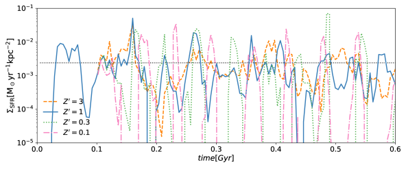
Figure 2: Time evolution of the star formation rate (SFR) surface density averaged over the entire simulation domain (face-on). Our $Z^{\prime}=1$ run agrees very well with the observed value in the solar neighborhood from Fuchs et al. (2009) shown as the horizontal black dotted line. The time-averaged SFR is insensitive to $Z^{\prime}$ (see also Table 3), but the temporal fluctuation of SFR significantly increases as $Z^{\prime}$ decreases.

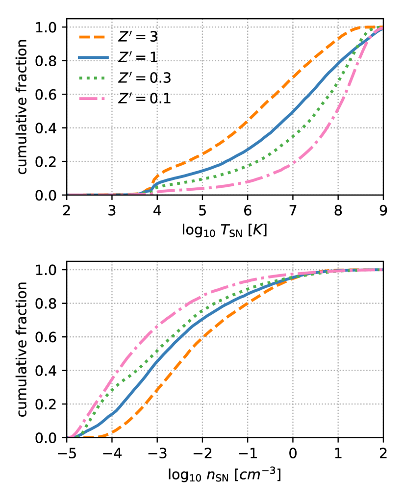
Figure 3: Cumulative distribution of the gas temperature ($T_{\rm SN}$, top panel) and hydrogen number density ($n_{\rm SN}$, bottom panel) where SNe occur. The vast majority of SNe go off in hot ($T_{\rm SN}>10^{5}$ K) and under-dense ($n_{\rm SN}<0.1{\rm cm^{-3}}$) regions, indicating that SNe are clustered and frequently go off in super-bubbles.

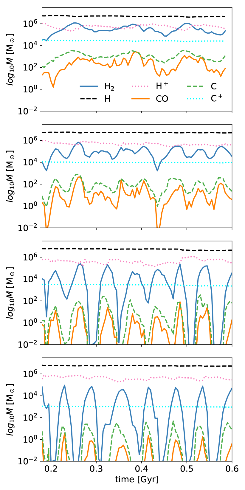
Figure 4: Total masses of H⁺, H, H₂, C⁺, C and CO in the time-dependent model as a function of time for $Z^{\prime}=$ 3, 1, 0.3 and 0.1 from top to bottom.

Fig. 2 shows the time evolution of the SFR surface density averaged over the entire simulation domain in the face-on projection at different metallicities. Our $Z^{\prime}=1$ run agrees very well with the observed value in the solar neighborhood, $\Sigma_{\rm SFR,0}=2.4\times 10^{-3}\ {\rm M_{\odot}\ yr^{-1}\ kpc^{-2}}$ (Fuchs et al., 2009, shown as the horizontal black dotted line). As demonstrated in several previous studies, the key to this success is the proper inclusion of stellar feedback (see, e.g., Gatto et al., 2017; Kim & Ostriker, 2017; Hopkins et al., 2018). In fact, the time-averaged SFR is rather insensitive to $Z^{\prime}$ (see also Table 3). However, the temporal fluctuation of SFR is significantly larger at lower $Z^{\prime}$, partly because the fine-structure metal-line cooling rate is linearly proportional to $Z^{\prime}$. Once the cold clouds are destroyed and heated up by stellar feedback, it takes longer for the gas to cool down from $10^{4}$ K, which delays the gravitational collapse and star formation. Another reason for the burstiness is that star formation occurs at increasingly higher densities as $Z^{\prime}$ decreases because the clouds are slightly warmer (as will be shown below). Consequently, the SFR is elevated locally, which explains the higher peaks, and the subsequent stellar feedback is more clustered and destroys clouds more efficiently. The absolute burstiness is expected to depend on the box size, as different patches of the ISM may be in different phases of the fluctuation in a real galaxy. However, the systematic trend with metallicity should be robust.

Fig. 3 shows the cumulative distribution of the gas temperature ($T_{\rm SN}$, top panel) and hydrogen number density ($n_{\rm SN}$, bottom panel) where SNe occur at different metallicities. The vast majority of SNe explode in hot ($T_{\rm SN}>10^{5}$ K) and under-dense ($n_{\rm SN}<0.1{\rm cm^{-3}}$) regions, indicating that SNe are clustered and frequently go off in super-bubbles. Furthermore, as metallicity decreases, $T_{\rm SN}$ increases while $n_{\rm SN}$ decreases. SNe are more clustered at lower metallicities, which leads to more efficient feedback and thus burstier SFRs.

Fig. 4 shows the total masses of H⁺, H, H₂, C⁺, C and CO as a function of time for $Z^{\prime}=$ 3, 1, 0.3 and 0.1 from top to bottom. Most hydrogen is in the form of H while most carbon is in the form of C⁺, both of which remain almost constant with time. In contrast, the masses of H₂, C and CO show significant time variations as they trace the cold and dense gas and their modulation is correlated with the SFR. The H⁺ mass anti-correlates with the cold-gas tracers (H₂, C and CO) as H⁺ is generated primarily by supernovae and photoionization. Therefore, it peaks at the “destruction” phase of the ISM cycles when the cold-gas tracers are at their minima.

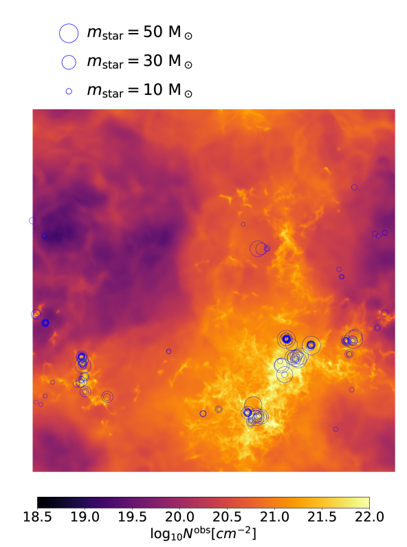
Figure 5: Column density map of total hydrogen at $t=530$ Myr in the $Z^{\prime}=1$ run (solar metallicity). Massive stars are overplotted as the blue circles (sizes are scaled with the stellar masses).

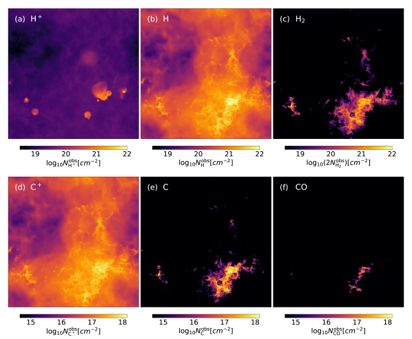
Figure 6: Column density maps of (a) ionized hydrogen, (b) atomic hydrogen, (c) molecular hydrogen, (d) ionized carbon, (e) atomic carbon, and (f) carbon monoxide at $t=530$ Myr in the $Z^{\prime}=1$ run (solar metallicity).

For a visual impression, Fig. 5 shows the observed column density maps of total hydrogen at $t=530$ Myr in the $Z^{\prime}=1$ run, which is designed to be a model for the solar neighborhood. The entire simulation domain of 1 kpc² is shown. A multi-phase hierarchical structure is evident, and consists of dense molecular clouds, a diffuse medium and SN-driven cavities. Massive stars are overplotted as the blue circles (sizes are scaled with the stellar masses). They are spatially clustered, especially for the more massive ones, and mostly located within the dense clouds. Fig. 6 shows the observed column density maps of H⁺, H, H₂, C⁺, C and CO from panel (a) to (f), respectively, for the same snapshot as Fig. 5. Recent feedback events are traced by the small bubbles in the H⁺ map. Carbon is mostly in the form of C⁺ in the volume-filling diffuse medium. H₂ is a tracer for dense clouds while CO traces the even denser part of the clouds. The atomic carbon is an intermediate phase between C⁺ and CO. Qualitatively, the chemical properties of the ISM are broadly consistent with standard PDR calculations (van Dishoeck & Black, 1988; Sternberg & Dalgarno, 1995; Röllig et al., 2007; Bisbas et al., 2017).

Given the strong temporal variations, any analysis for a particular snapshot will be biased and incomplete. As such, in the following sections, all results we present will be “time-averaged” over the snapshots between 150 and 600 Myr with a time interval of 5 Myr (91 snapshots in total) for each simulation. For a histogram (either 1D or 2D), time-averaging is simply done bin by bin over all snapshots. A cumulative distribution is generated from the time-averaged histogram (which is different from time-averaging 91 cumulative distributions bin-wise). A correlation plot between $x$ and $y$ that shows the median of $y$ in each $x$-bin by a line (and sometimes also the scatter of $y$ by a shaded area) is constructed from a time-averaged 2D histogram of $x$ and $y$. By doing so, the temporal and spatial scatters are treated on an equal footing and can be shown simultaneously. Each snapshot can also be viewed equivalently as a different patch of a galaxy.

4.2 Thermodynamical properties

Figure 7: Time-averaged 2D histograms of density vs. temperature for $Z^{\prime}=$ 3, 1, 0.3 and 0.1 from left to right. The red dashed lines represent the median temperature within each density bin. The white solid lines indicate the star formation threshold where $M_{\rm J}=32\ {\rm M_{\odot}}$. The slightly higher temperature in the cold phase at lower $Z^{\prime}$ shift star formation to higher densities.

Fig. 7 shows the time-averaged 2D histograms of $n$ vs. $T$ for $Z^{\prime}=$ 3, 1, 0.3 and 0.1 from left to right. The red dashed lines represent the median temperature within each density bin. The white solid lines indicate the star formation threshold where $M_{\rm J}=32\ {\rm M_{\odot}}$. The overall gas distribution broadly follows the classical curves for bistable warm/cold thermal equilibrium. The scatter increases with decreasing $Z^{\prime}$ as the bursty SFR implies large temporal variations of $I_{\rm UV}$ and $\zeta_{\rm CR}$, which in turn alter the thermal-equilibrium curves. In addition, the hot gas ($T>10^{5}$ K) is generated by SN feedback while the narrow gas distribution at $T=10^{4}$ K and $n_{\rm H}>10\ {\rm cm^{-3}}$ originates from photoionization in the HII regions. The majority of gas is in the warm and diffuse phase ($T\sim 10^{4}$ K and $n\sim 1\ {\rm cm^{-3}}$) whose temperature is rather insensitive to $Z^{\prime}$ as it is controlled by the Lyman alpha cooling. In contrast, the cold and dense phase ($T<10^{2}$ K and $n>10\ {\rm cm^{-3}}$) has a typical temperature that is slightly higher at lower $Z^{\prime}$. This is partly due to less efficient dust shielding that enhances photoelectric heating, and, at the highest densities, due to heating from UV pumping and H₂ formation (Bialy & Sternberg, 2019). As such, gas has to collapse to higher densities to reach the same level of gravitational instability (quantified by $M_{\rm J}$) to form stars, making the SFR burstier at lower $Z^{\prime}$ as discussed above.

To be more quantitative, Fig. 8 shows the time-averaged mass-weighted histograms of $n$ (left) and $T$ (right) at different metallicities. The density histogram peaks at $n\sim 1\ {\rm cm^{-3}}$ which represents the typical density of the diffuse background medium. At higher metallicities ($Z^{\prime}=$ 3 and $Z^{\prime}=$ 1), the two-phase feature due to thermal instability (Field et al., 1969; Wolfire et al., 2003; Bialy & Sternberg, 2019) is clearly visible with two distinct peaks at $T\sim 10^{4}$ K and $T\sim 10^{2}$ K in the temperature histogram. At lower metallicities ($Z^{\prime}=$ 0.3 and $Z^{\prime}=$ 0.1), the cold phase is less prominent and more gas can be found in the unstable intermediate temperature regime. This occurs because the cooling time becomes comparable to or longer than the dynamical time at low $Z^{\prime}$ and so the gas is constantly driven away from its thermally stable phases.

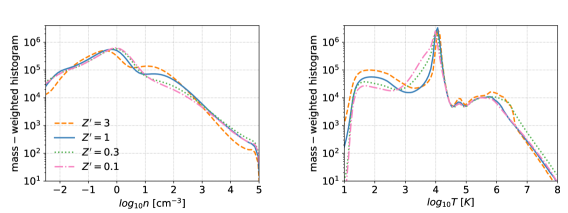
Figure 8: Time-averaged mass-weighted histograms of density (left) and temperature (right) at different metallicities. The two-phase feature due to thermal instability is more pronounced at high $Z^{\prime}$.

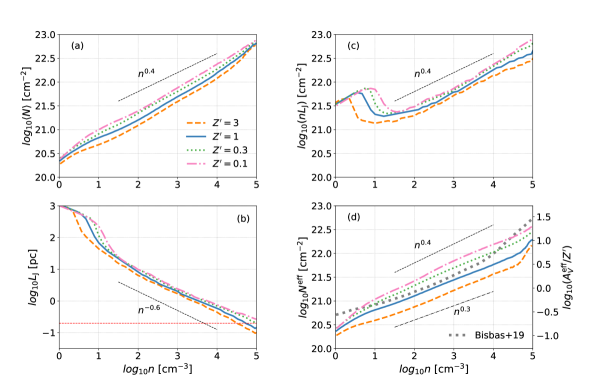
Figure 9: (a) Angle-averaged (geometric mean) hydrogen column density $\langle N\rangle$ as a function of $n$ at different metallicities. The black dashed line indicates a power-law relation of $n^{0.4}$. (b) Same as (a), but showing the local Jeans length $L_{\rm J}$ on the $y$-axis. The black dashed line indicates a power-law relation of $n^{-0.6}$, and the horizontal red dashed line shows the adopted gravitational softening length $\epsilon_{\rm soft}=$ 0.2 pc. (c) Same as (a), but showing $nL_{\rm J}$ on the $y$-axis. (d) Same as (a), but showing the effective column density $N^{\rm eff}$ (i.e., angle-averaged via Eq. 12) on the $y$-axis. The corresponding $A_{V}/Z^{\prime}$ is shown on the right $y$-axis. The grey dotted line shows the average of four independent hydrodynamical simulations with solar-metallicity in the literature as compiled by Bisbas et al. (2019). All quantities are time-averaged.

4.3 Correlation between $n$ and $N^{\rm eff}$

The amount of available shielding material against the FUV radiation is an important factor for the formation of H₂ and CO. Panel (a) in Fig. 9 shows the angle-averaged geometric mean of the hydrogen column density $\langle N\rangle$ (see Eq. 13) as a function of $n$. The geometric mean roughly scales as $n^{0.4}$ (the black dashed line) and is insensitive to $Z^{\prime}$ besides a slight difference in normalization. Panel (b) in Fig. 9 shows the thermal Jeans length $L_{\rm J}=\sqrt{\pi c_{s}^{2}/(G\rho)}$ as a function of $n$. Our adopted gravitational softening length $\epsilon_{\rm soft}=$ 0.2 pc is shown by the horizontal red dashed line in panel (b), which represents the minimum length scale at which the gravity can be resolved. All snapshots are combined and the median values are shown.

In the cold and dense phase $n>30\ {\rm cm^{-3}}$, the temperature decreases very slowly as density increases (“isothermal regime”), which leads to $L_{\rm J}\propto n^{-0.6}$. Assuming the Jeans length is the typical cloud size at a given density, we can estimate the hydrogen column density by $nL_{\rm J}$, which is shown in panel (c) of Fig. 9 as a function of $n$ and agrees well with $\langle N\rangle$ in panel (a) in the range of $10<n<10^{4}\ {\rm cm^{-3}}$, suggesting that the correlation between $n$ and $\langle N\rangle$ is a consequence of gravitational instability. This Jeans-length argument has been demonstrated by Rahmati et al. (2013) and Safranek-Shrader et al. (2017). However, we caution that Glover et al. (2010) found a similar correlation in their turbulent box simulations without self-gravity, implying that the Jeans-length argument might also be a coincidence. The correlation is insensitive to $Z^{\prime}$ because the relationship between density and temperature (and thus the Jeans length) is insensitive to $Z^{\prime}$ (see Fig. 7). At a given density, $\langle N\rangle$ is only slightly larger at lower $Z^{\prime}$ as the temperature is higher. At $n<10\ {\rm cm^{-3}}$, there is a sudden increase in $nL_{\rm J}$ corresponding to the abrupt transition from $T\sim 100$ K to $T\sim 10^{4}$ K. The same jump is not seen in $\langle N\rangle$, as the warm and diffuse medium is gravitationally stable against its self-gravity (otherwise the entire disk would have been collapsing) and thus gas does not cluster on a scale of $L_{\rm J}$.

Note that our adopted shielding length $L_{\rm sh}=100$ pc is much larger than the Jeans length of the clouds. Therefore, we expect $nL_{\rm J}$ to be a lower limit of $\langle N\rangle$ even if $L_{\rm J}$ is a good proxy of the typical cloud size, as material beyond $L_{\rm J}$ and up to $L_{\rm sh}$ to can still make a contribution. The good agreement found between $nL_{\rm J}$ and $\langle N\rangle$ suggests that this contribution is not very important and the majority of shielding occurs in the vicinity of the clouds. We explore different choices of $L_{\rm sh}$ in Appendix B.1.

On the other hand, in terms of dust shielding of H₂ and CO, the more relevant quantity is the effective column density $N^{\rm eff}$ (see Eq. 12) rather than $\langle N\rangle$. Although $N^{\rm eff}$ is also an angle average like $\langle N\rangle$, it has a different weighting that is biased towards pixels with the lowest column densities. Therefore, $N^{\rm eff}$ roughly corresponds to the optical depth of a cloud. From Eq. 12, pixels with $A_{V,i}\gg 1$ where dust shielding becomes effective are significantly down-weighted, which corresponds to a lower $N_{i}$ at higher $Z^{\prime}$. Therefore, in Panel (d) of Fig. 9 where we show $n$ vs. $N^{\rm eff}$, we see the curves are down-shifted and flattened compared to panel (a), to a larger extent at higher $Z^{\prime}$. The grey dotted line shows the average of four independent hydrodynamical simulations at solar-metallicity in the literature, Glover et al. (2010), Van Loo et al. (2013), Safranek-Shrader et al. (2017) and Seifried et al. (2017), as compiled by Bisbas et al. (2019). Our $Z^{\prime}=1$ run agrees very well with those simulations in the range of $10<n<10^{4}\ {\rm cm^{-3}}$. Above this density range, the Jeans length drops below our resolution limit and thus gravity becomes underestimated (softened), which presumably explains the discrepancy. Quantitatively, we find the correlation can be well-described by

$$N^{\rm eff}=A(n/{\rm cm^{-3}})^{\alpha}$$ (14)

where $A/(10^{20}{\rm cm^{-2}})=$ 2, 3, 4 and 4.5 while $\alpha=$ 0.3, 0.33, 0.36 and 0.39 for $Z^{\prime}=$ 3, 1, 0.3 and 0.1, respectively.

Table 1: Densities, effective column densities and effective visual extinctions (see Eq. 12) at which H/H₂, C⁺/C and C/CO conversions occur in the time-dependent H₂ model.

$Z^{\prime}$	$n^{*}_{\rm H_{2}}$	$n^{*}_{\rm C}$	$n^{*}_{\rm CO}$	$N^{*}_{\rm H_{2}}$	$N^{*}_{\rm C}$	$N^{*}_{\rm CO}$	$A^{*}_{V,{\rm H_{2}}}$	$A^{*}_{V,{\rm C}}$	$A^{*}_{V,{\rm CO}}$
	$[{\rm cm^{-3}}]$	$[{\rm cm^{-3}}]$	$[{\rm cm^{-3}}]$	$[{\rm 10^{21}cm^{-2}}]$	$[{\rm 10^{21}cm^{-2}}]$	$[{\rm 10^{21}cm^{-2}}]$
3	90	68	720	0.88	0.78	1.7	1.4	1.2	2.7
1	470	270	3100	2.9	2.1	4.6	1.5	1.1	2.5
0.3	3300	1400	14000	9.4	7.2	14	1.5	1.2	2.2
0.1	16000	6800	69000	22	16	34	1.2	0.87	1.8

Note. — (1) Normalized metallicity; (2)-(4) Conversion densities for H/H₂, C⁺/C, and C/CO, respectively. (5)-(7) Conversion effective column densities for H/H₂, C⁺/C, and C/CO, respectively. (8)-(10) Conversion effective visual extinctions for H/H₂, C⁺/C, and C/CO, respectively.

Table 2: Same as Table 1 but in the steady-state H₂ model.

$Z^{\prime}$	$n^{*}_{\rm H_{2}}$	$n^{*}_{\rm C}$	$n^{*}_{\rm CO}$	$N^{*}_{\rm H_{2}}$	$N^{*}_{\rm C}$	$N^{*}_{\rm CO}$	$A^{*}_{V,{\rm H_{2}}}$	$A^{*}_{V,{\rm C}}$	$A^{*}_{V,{\rm CO}}$
	$[{\rm cm^{-3}}]$	$[{\rm cm^{-3}}]$	$[{\rm cm^{-3}}]$	$[{\rm 10^{21}cm^{-2}}]$	$[{\rm 10^{21}cm^{-2}}]$	$[{\rm 10^{21}cm^{-2}}]$
3	11	66	620	0.43	0.78	1.6	0.69	1.2	2.5
1	33	270	2400	0.97	2.1	4.1	0.52	1.1	2.2
0.3	68	1400	11000	2.1	7.2	12	0.34	1.2	2.0
0.1	200	6500	54000	5.2	16	30	0.28	0.85	1.6

4.4 Atomic-molecular distributions

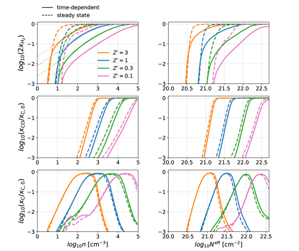
Figure 10: Time-averaged normalized fractional chemical abundances of H₂ ($2x_{\rm H_{2}}$, top panel), CO ($x_{\rm CO}/x_{\rm C,0}$, middle panel) and C ($x_{\rm C}/x_{\rm C,0}$, bottom panel) as a function of $n$ (left) and $N^{\rm eff}$ (right) at different metallicities. The time-dependent H₂ model is shown in solid lines while the steady-state H₂ model is shown in dashed lines. The thin dotted lines in the top left panel show the analytic solutions (Eq. 16). The time-dependent effect makes the H₂ abundance profile much shallower than its steady-state counterpart.

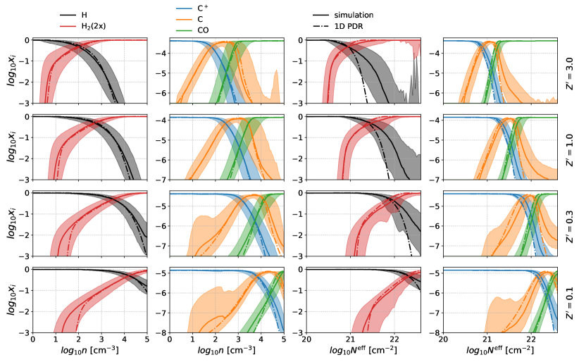
Figure 11: Chemical abundances of H (black), H₂ (red, multiplied by 2), C⁺ (blue), C (orange) and CO (green) for the time-dependent H₂ model as a function of $n$ (1st and 2nd columns) and $N^{\rm eff}$ (3rd and 4th columns) for $Z^{\prime}=$ 3, 1, 0.3 and 0.1 from top to bottom. The solid lines show the medium abundances in each $n$- and $N^{\rm eff}$-bin while the shaded area brackets the 16 and 84 percentiles. The dash-dotted lines show the effective 1D PDR model, which agrees remarkably well with the median abundances in simulations.

Figure 12: Schematic illustration of a typical cloud and its chemical composition at increasing metallicity from right to left. Top: the steady-state model. The transitions of H/H₂, C⁺/C and C/CO occur at the boundaries of the white/purple, purple/red and red/magenta, respectively. The transition surfaces are sharp and well-defined. As the metallicity decreases, the C⁺/C and C/CO surfaces contract faster than the H/H₂ surface. Bottom: the time-dependent model. The C⁺/C and C/CO transitions are largely unchanged. The H₂ abundance shows a shallow radial profile which declines gradually with increasing radius up to the sharp H₂ photodissociation front.

Having discussed the gas densities and thermal states, we now present the chemical compositions focusing on the atomic-to-molecular conversions. Fig. 10 shows the normalized fractional chemical abundances of H₂ ($2x_{\rm H_{2}}$, top panel), CO ($x_{\rm CO}/x_{\rm C,0}$, middle panel) and C ($x_{\rm C}/x_{\rm C,0}$, bottom panel) as functions of $n$ (left) and $N^{\rm eff}$ (right) for different metallicities. The time-dependent H₂ model is shown in solid lines while the steady-state H₂ model is shown in dashed lines. In addition, we define conversion densities for H₂ ($n^{*}_{\rm H_{2}}$), C ($n^{*}_{\rm C}$) and CO ($n^{*}_{\rm CO}$) as the densities where $x_{\rm H}=2x_{\rm H_{2}}$, $x_{\rm C^{+}}=x_{\rm C}$, and $x_{\rm C}=x_{\rm CO}$, respectively. Likewise, the conversion (effective) column densities of H₂ ($N^{*}_{\rm H_{2}}$), C ($N^{*}_{\rm C}$) and CO ($N^{*}_{\rm CO}$) are defined in a similar fashion, with the associated conversion visual extinctions $A^{*}_{V,{\rm H_{2}}}$, $A^{*}_{V,{\rm C}}$ and $A^{*}_{V,{\rm CO}}$, respectively. These quantities are summarized in Tables 1 and 2.

Our steady-state H₂ model is qualitatively consistent with standard PDR expectations. The abundance profiles of H₂ and CO are both shifted towards higher $n$ and $N^{\rm eff}$ at decreasing $Z^{\prime}$ (recall that $N^{\rm eff}$ is roughly a monotonically increasing function of $n$). At any given metallicity, the H/H₂ conversion occurs at the lowest density and column density, then followed by C⁺/C and C/CO as the column density increases. These profiles are mainly determined by a balance between the formation via two-body reactions and the destruction via photodissociation or photoionization. The sharp conversions occur when the accumulated column densities are such that enough FUV radiation is attenuated. At the conversion density of H₂, the corresponding dimensionless parameter $\alpha G$ from Sternberg et al. (2014) (their Eqs. 44 and 46), which quantifies the relative importance between dust-shielding and self-shielding, is 2.7, 0.91, 0.44 and 0.15 for $Z^{\prime}=$ 3, 1, 0.3 and 0.1, respectively. Therefore, self-shielding becomes increasingly important at decreasing $Z^{\prime}$.

In contrast, in the more realistic time-dependent H₂ model, the H₂ profile is much shallower, spanning almost two orders of magnitude in $n$ from $2x_{\rm H_{2}}=0.1$ to $2x_{\rm H_{2}}=1$. In addition, the H/H₂ conversions occur at much higher densities than their steady-state counterparts, by a factor of 8, 14, 39 and 64 for $Z^{\prime}=$ 3, 1, 0.3 and 0.1, respectively. In other words, H₂ is further away from steady state at lower $Z^{\prime}$. This is expected as $t_{\rm H_{2},form}\propto 1/Z^{\prime}$ becomes progressively longer than the dynamical time $t_{\rm dyn}$, defined here as the available time for which H₂ can form unperturbed. We expect $t_{\rm dyn}$ to be insensitive to $Z^{\prime}$ as it is mainly controlled by the SFR (via stellar feedback) which is insensitive to $Z^{\prime}$ in our simulations. Empirically, we find the dynamical time in the following form

$$t_{\rm dyn}=3\ {\rm Myr}\ n_{2}^{-0.3},$$ (15)

where $n_{2}\equiv n/(100\ {\rm cm^{-3}})$, can explain the H₂ abundances in the well-shielded regions

$$2x_{\rm H_{2}}=1-e^{-t_{\rm dyn}/t_{\rm H_{2},form}}=1-e^{-0.2Z_{d}^{\prime}n_{2}^{0.7}},$$ (16)

which is over-plotted in the upper left panel of Fig. 10 as the thin dotted lines. This simple analytic expression captures the average H₂ profile for the time-dependent model at all metallicities remarkably well, except for the outermost part where the H₂ profile is truncated and overlaps with the profiles for the steady-state model, which serve as an upper limits for the former. In short, the H/H₂ conversions are dictated mainly by the available time for H₂ formation, which results in a slowly declining profile up to the surface of the sharp photodissociation front.

In comparison, C/CO conversions occur at much higher densities with $n^{*}_{\rm CO}\approx 5n^{*}_{\rm H_{2}}$. Moreover, unlike the H₂ profiles, the CO profiles agree well with their steady-state counterparts, which is not trivial as both the formation and destruction of CO are affected by the presence of H₂. However, in both models, hydrogen is already fully molecular where the C/CO conversions occur, which implies the same CO formation rates. The difference in the H₂ profiles in both models does lead to a difference in the H₂ column densities which is very significant at low $Z^{\prime}$. However, as the C/CO conversions occur at much higher densities than H/H₂, the effective H₂ column densities relevant for shielding are quite similar in both models. Therefore, it turns out that the time-dependent effect only shifts the C/CO conversions towards marginally higher density and column density.

Finally, the time-dependent effect has the least impact on the C⁺/C conversions. This is expected as these are largely determined by the photoionization of C and recombination of C⁺ (either radiative or on grains), which has little to do with H₂ per se. Interestingly, the H/H₂ conversions occur (becomes half-molecular) at slightly higher column densities than C⁺/C in the time-dependent case, which is contrary to the steady-state model.

4.5 Effective 1D PDR model

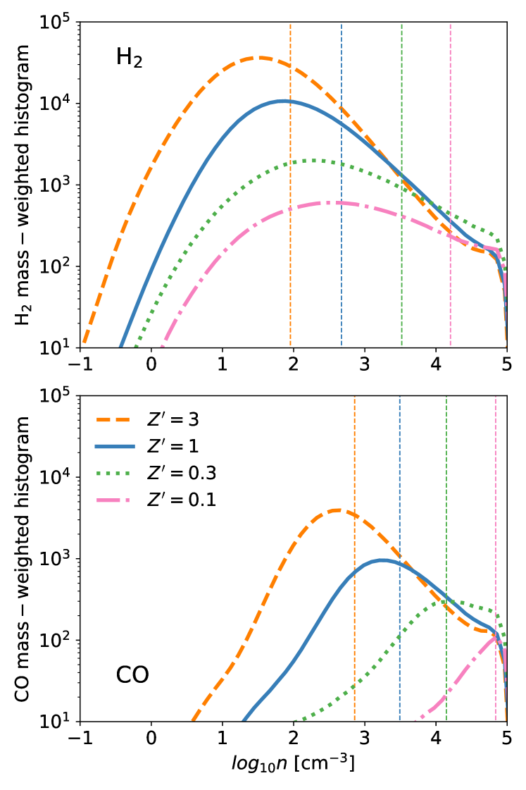
Figure 13: Time-averaged density histograms weighted by the H₂ mass ($2m_{\rm g}x_{\rm H_{2}}$, top panel) and normalized CO mass ($28m_{\rm g}x_{\rm CO}/x_{\rm C,0}$, bottom panel) at different metallicities. The vertical lines indicate the conversion densities as shown in Table 1. The majority of H₂ is found at a density much lower than the H₂ conversion density (see Table 1).

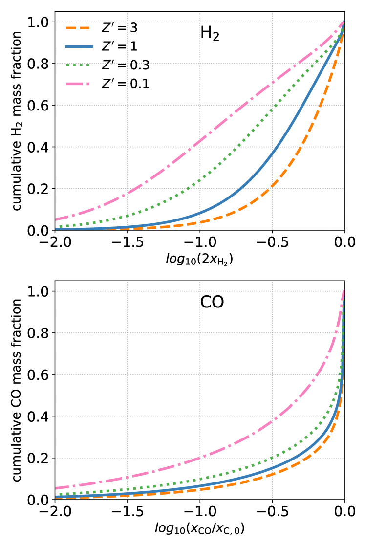
Figure 14: Time-averaged cumulative molecular mass fraction as a function of normalized chemical abundance at different metallicities. The top and bottom panels are for H₂ and CO, respectively. A significant fraction of the H₂ mass is found in low-H₂ abundance gas.

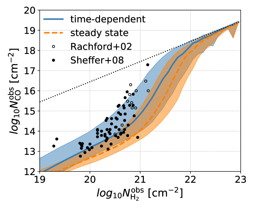
Figure 15: Time-averaged $N^{\rm obs}_{\rm H_{2}}$ - $N^{\rm obs}_{\rm CO}$ relationship in the $Z^{\prime}=1$ run. The blue solid line shows the time-dependent H₂ model while the orange dashed line shows the steady-state H₂ model. The shaded area brackets the 16 and 84 percentiles in each $N^{\rm obs}_{\rm H_{2}}$-bin. The black circles are observational data from Rachford et al. (2002) (empty) and Sheffer et al. (2008) (filled) for Galactic diffuse clouds. The dotted grey line indicates the upper limit for $N^{\rm obs}_{\rm CO}$ when all carbon is in the form of CO.

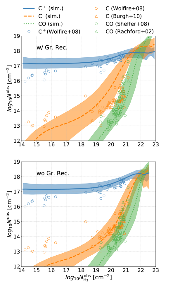
Figure 16: Time-averaged relationships of $N^{\rm obs}_{\rm H_{2}}$ vs. $N^{\rm obs}_{\rm C^{+}}$ (solid blue), $N^{\rm obs}_{\rm C}$ (dashed orange) and $N^{\rm obs}_{\rm CO}$ (dotted green) in the $Z^{\prime}=1$ run. The lines show the median values while the shaded areas bracket the 16 and 84 percentiles. The top and bottom panels are models with and without recombination on grains, respectively (both models are time-dependent). Observational data of the Galactic clouds are taken from Wolfire et al. (2008) (blue circles for C⁺ and orange circles for C), Burgh et al. (2010) (orange triangles for C), Sheffer et al. (2008) (green circles for CO) and Rachford et al. (2002) (green triangles for CO). Switching off recombination on grains leads to better agreement with the observed $N^{\rm obs}_{\rm C}$ except for the low-column density regime where both models under-produce the atomic carbon.

The relationships in Fig. 10 are averaged over a large ensemble of clouds both spatially and temporally and therefore are representative of the abundance distributions of typical clouds (although smaller clouds may not have the depth to reach the highest $N^{\rm eff}$). In fact, we can construct an effective 1D PDR model that represents these distributions as follows. Assuming the cloud follows a power-law density profile $n(x)=Bx^{\beta}$, where $x=0$ is the cloud center while the external radiation is illuminated from $\infty$. Adopting a 1D slab geometry, the column density integrated from $\infty$ to $x$ is $N(x)\equiv-\int_{\infty}^{x}n(x^{\prime})dx^{\prime}=-Bx^{\beta+1}/(\beta+1)$. Meanwhile, the column density is correlated with $n$ (see Eq. 14) such that $N(x)=An(x)^{\alpha}=AB^{\alpha}x^{\alpha\beta}$. Therefore, it follows that $\beta=1/(\alpha-1)$ and $B=(A\alpha/(1-\alpha))^{1/(1-\alpha)}$.

We now can conduct 1D PDR calculations with this effective cloud profile, evolving up to $t_{\rm dyn}$ at each density bin to capture the time-dependent effect. We adopt $I_{\rm UV}=1$ and $\zeta_{\rm CR}=10^{16}\ {\rm s^{-1}}$ as the time-averaged SFR is close to the solar-neighborhood value at all metallicities. The temperature is fixed at 20 K as we find that the results are insensitive to moderate variations of temperature. The results are compared with simulations in Fig. 11, which shows the chemical abundances of H (black), H₂ (red, multiplied by 2), C⁺ (blue), C (orange) and CO (green) in the time-dependent model as functions of $n$ (1st and 2nd columns) and $N^{\rm eff}$ (3rd and 4th columns) for $Z^{\prime}=$ 3, 1, 0.3 and 0.1 from top to bottom. The solid lines show the medium abundances in each $n$- and $N^{\rm eff}$-bin while the shaded area brackets the 16 and 84 percentiles. The dash-dotted lines show the effective 1D PDR model, which agrees remarkably well with the median abundances in simulations. There are some discrepancies in $N^{\rm eff}$ vs. $x_{\rm H}$ in the H₂-dominated regimes despite the agreement in the corresponding $n$ vs. $x_{\rm H}$, suggesting that the discrepancies originate from the $n-N^{\rm eff}$ relationship. This is expected as $N^{\rm eff}$ represents, by definition, the amount of dust shielding for CO and thus might not be a perfect proxy for H₂ self-shielding.

In Fig. 12, we provide a schematic illustration of the effective cloud and its chemical composition at increasing metallicity from right to left. The top row shows the standard steady-state model (Bolatto et al., 2013). The transitions of H/H₂, C⁺/C and C/CO occur at the boundaries of the white/purple, purple/red and red/magenta, respectively. The transition surfaces are sharp and well-defined. As the metallicity decreases, the C⁺/C and C/CO surfaces contract faster than the H/H₂ surface as H₂ self-shielding is very efficient. In contrast, the bottom row shows the time-dependent model, where the H₂ abundance shows a shallow radial profile which declines gradually with increasing radius up to the sharp H₂ photodissociation front. At low $Z^{\prime}$, photodissociation has almost no effect on the H₂ profile as H₂ formation is mainly limited by the dynamical processes. The C⁺/C and C/CO transitions are largely unchanged.

4.6 Density distributions of H₂ and CO

Fig. 13 shows the histograms of $n$ weighted by the H₂ mass ($2m_{\rm g}x_{\rm H_{2}}$, top panel) and normalized CO mass ($28m_{\rm g}x_{\rm CO}/x_{\rm C,0}$, bottom panel). The vertical lines indicate the conversion densities as shown in Table 1.

Most CO is found at $n\sim n^{*}_{\rm CO}$ (as indicated by the peak of the histogram), while most H₂ is found at a density much lower than $n^{*}_{\rm H_{2}}$. This is due to the difference in their profile shapes, as the molecular mass-weighted density histogram is essentially a convolution of the total gas density histogram with the abundance profile. Therefore, the sharp CO profile means that most CO lives at $n\gtrsim n^{*}_{\rm CO}$, while the shallow H₂ profile means that gas with density below $n^{*}_{\rm H_{2}}$ can still make a significant contribution to the total H₂ mass budget, shifting the peak towards a much lower density. This can be more quantitatively demonstrated by the cumulative molecular mass fraction as a function of the normalized molecular abundance shown in Fig. 14. The top and bottom panels are for H₂ and CO, respectively. While most of the CO mass originates from gas with high $x_{\rm CO}$, a significant fraction of the H₂ mass can be found in HI-dominated gas. This is most prominent at $Z^{\prime}=0.1$, where the shallow H₂ profile spans almost four orders of magnitude in $n$ before being truncated at the photodissociation surface, and thus more than 40% of H₂ is found in gas with $2x_{\rm H_{2}}<0.1$.

4.7 Comparison with the observed Galactic clouds

The fact that H₂ is significantly affected by the time-dependent effect while CO is not leads to an interesting observational consequence. Fig. 15 shows the $N^{\rm obs}_{\rm H_{2}}$ - $N^{\rm obs}_{\rm CO}$ relationship in the $Z^{\prime}=1$ run. The blue solid line shows the time-dependent H₂ model while the orange dashed line shows the steady-state H₂ model. The shaded area brackets the 16 and 84 percentiles in each $N^{\rm obs}_{\rm H_{2}}$-bin. The black circles are observational data from Rachford et al. (2002) (empty) and Sheffer et al. (2008) (filled) for Galactic diffuse clouds. The dotted grey line indicates the upper limit for $N^{\rm obs}_{\rm CO}$ when all carbon is in the form of CO. Our time-dependent H₂ model agrees well with observations especially in the low-column density regime, which gives us confidence that our model is reasonably realistic. In contrast, since the steady-state H₂ model generally over-produces H₂ but not CO, the results are shifted rightward and away from the observed data. This is an intriguing demonstration of how the time-dependent effect helps explain the observed $N^{\rm obs}_{\rm H_{2}}$ - $N^{\rm obs}_{\rm CO}$ relationship without resorting, for example, to non-thermal velocity distributions (boosted by the Alfvén waves) for the reaction C⁺ + H₂ $\rightarrow$ CH⁺ + H (e.g. Federman et al., 1996; Sheffer et al., 2008; Visser et al., 2009), which we do not include. That said, it does not negate the need for this reaction to produce CH⁺ given the widespread observations of CH⁺ in the diffuse medium. We note that Gong et al. (2018) have also reproduced the observed $N^{\rm obs}_{\rm H_{2}}-N^{\rm obs}_{\rm CO}$ relationship in their simulations. However, they assumed steady-state chemistry which tends to over-produce H₂, and it remains to be seen whether their results still hold if they account for the time-dependent effect.

Fig. 16 shows the time-averaged relationships of $N^{\rm obs}_{\rm H_{2}}$ vs. $N^{\rm obs}_{\rm C^{+}}$ (solid blue), $N^{\rm obs}_{\rm C}$ (dashed orange) and $N^{\rm obs}_{\rm CO}$ (dotted green) in the $Z^{\prime}=1$ run. The lines show the median values while the shaded areas bracket the 16 and 84 percentiles. The top and bottom panels are models with and without recombination on grains, respectively (both models are time-dependent). Observational data of the Galactic clouds are taken from Wolfire et al. (2008) (blue circles for C⁺ and orange circles for C), Burgh et al. (2010) (orange triangles for C), Sheffer et al. (2008) (green circles for CO) and Rachford et al. (2002) (green triangles for CO). Both models under-produces $N^{\rm obs}_{\rm C}$ in the low-column density regime where $10^{14}<N^{\rm obs}_{\rm H_{2}}/({\rm cm^{-2}})<10^{16}$. Our fiducial model (top panel) largely reproduces the observed $N^{\rm obs}_{\rm C^{+}}$ and $N^{\rm obs}_{\rm CO}$, but over-produces $N^{\rm obs}_{\rm C}$ by about a factor of ten in the regime where $N^{\rm obs}_{\rm H_{2}}>10^{19}{\rm cm^{-2}}$. Switching off recombination on grains reduces $N^{\rm obs}_{\rm C}$ down to the observed values without hampering the agreement in $N^{\rm obs}_{\rm C^{+}}$ and $N^{\rm obs}_{\rm CO}$. Despite the good agreement with observations, we refrain from making it our default model as there is no physically justified reason to switch off recombination on grains. Our results are consistent with Glover & Clark (2012b) who showed that the C/CO ratio in their turbulent box simulations agrees with the observed values when recombination on grains is switched off but is overestimated otherwise. On the other hand, Gong et al. (2017) found conflicting results in their PDR calculations where the C/CO ratio is overestimated either with or without recombination on grains. This is presumably because their CO abundances are significantly reduced without recombination on grains, which is not the case in our simulations (see Sec. B.2).

4.8 Global properties and CO-dark H₂ fraction

We now present the time-averaged global properties of the simulations which are summarized in Tables 3 and 4. $M_{\rm gas}$ is the total gas mass (including helium and metals) and $F_{100}$ is the mass fraction with $n>100\ {\rm cm^{-3}}$. The total mass of species $i$ is denoted as $M_{i}$ where $i$ = H⁺, H, H₂, C⁺, C and CO, while the mass fraction relative to the total hydrogen mass $M_{\rm H,0}=X_{\rm H}M_{\rm gas}$ is defined as $F_{i}=M_{i}/M_{\rm H,0}$. $F^{*}_{\rm dark}{\rm(CO)}$ is the mass fraction of the CO-dark H₂ gas (see details below). Fig. 17 shows $F_{\rm H^{+}}$, $F_{\rm H}$ and $F_{\rm H_{2}}$ in the left panel, $F_{\rm C^{+}}$, $F_{\rm C}$ and $F_{\rm CO}$ in the middle panel, and the mass ratios $M_{\rm H_{2}}/M_{\rm C^{+}}$, $M_{\rm H_{2}}/M_{\rm C}$ and $M_{\rm H_{2}}/M_{\rm CO}$ in the right panel as a function of $Z^{\prime}$, respectively. The time-dependent H₂ model is shown in solid lines while the steady-state H₂ model is in dashed lines.

Both the SFR and $F_{100}$ are insensitive to $Z^{\prime}$, as the density distribution varies only weakly with $Z^{\prime}$. The global gas depletion time is $M_{\rm gas}/{\rm SFR}\approx 4$ Gyr, slightly lower than the typical value of 2 Gyr in typical nearby spiral galaxies (Bigiel et al., 2008; Leroy et al., 2008). $F_{\rm H^{+}}$ is also insensitive to $Z^{\prime}$ as H⁺ is mainly generated in the HII regions and the supernova remnants, which are tied to the SFR. As H₂ only contributes to a small fraction of the total hydrogen mass, $F_{\rm H}\approx 1-F_{\rm H^{+}}-F_{\rm H_{2}}$ is also insensitive to $Z^{\prime}$ ($\sim$ 90%). In the steady-state H₂ model, $F_{\rm H_{2}}$ scales sub-linearly with $Z^{\prime}$ because of the efficient H₂ self-shielding. However, in the time-dependent case, $F_{\rm H_{2}}$ scales roughly linearly with $Z^{\prime}$ as H₂ is mainly limited by the dynamical time especially at low $Z^{\prime}$. As such, the steady-state H₂ model significantly overestimates $F_{\rm H_{2}}$, by a factor of 1.8, 2.6, 6,3 and 11 for $Z^{\prime}=3$, 1, 0.3 and 0.1, respectively.

The vast majority ($\sim$ 99%) of carbon is in the form of C⁺, and thus $F_{\rm C^{+}}$ scales linearly with $Z^{\prime}$. Both $F_{\rm C}$ and $F_{\rm CO}$ scale super-linearly with $Z^{\prime}$, due to the effect of dust shielding in addition to the available carbon. Contrary to $F_{\rm H_{2}}$, $F_{\rm C}$ and $F_{\rm CO}$ are almost unaffected by the time-dependent effect as the C/CO conversions are only weakly affected by the over-estimated H₂. Therefore, the ratios $M_{\rm H_{2}}/M_{\rm CO}$ and $M_{\rm H_{2}}/M_{\rm C}$ still anti-correlate with $Z^{\prime}$, but not as much as what the steady-state H₂ model predicts. Interestingly, the ratios $M_{\rm H_{2}}/M_{\rm C^{+}}$ and $M_{\rm H_{2}}/M_{\rm C}$ both show a weaker dependence on $Z^{\prime}$ than $M_{\rm H_{2}}/M_{\rm CO}$. This indicates that they could potentially be viable tracers for H₂ at low $Z^{\prime}$, although a robust assessment requires information of the line intensities of these tracers, which we leave for future work.

As $F_{\rm H_{2}}$ decreases with $Z^{\prime}$ while the SFR is insensitive to $Z^{\prime}$, we confirm that the cold gas reservoir can be dominated by atomic hydrogen at low $Z^{\prime}$ as demonstrated by previous work (Krumholz, 2012; Glover & Clark, 2012c; Hu et al., 2016). Note that star formation occurs at $n\gtrsim 10^{4}-10^{5}\ {\rm cm^{-3}}$ which is above the H₂ conversion density. This means that even if the cold gas reservoir is dominated by atomic hydrogen, gas that undergoes runaway gravitational collapse will become molecular at some point before turning into stars. Therefore, our results that the cold gas reservoir is mostly atomic would still hold even if we were to adopt an H₂-based star formation recipe. We stress that this is the case only because we resolve the gravitational collapse up to very high densities. In cases where the H/H₂ conversion is unresolved (e.g. cosmological simulations), the H₂-based star formation recipe leads to inaccurate ISM properties and thus should not be used.

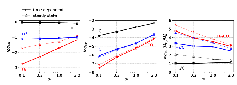
Figure 17: Time-averaged global chemical properties as a function of $Z^{\prime}$. Left: mass fractions of H⁺, H and H₂ relative to the total hydrogen mass. Middle: mass fractions of C⁺, C and CO relative to the total hydrogen mass. Right: mass ratio of H₂/C⁺, H₂/C and H₂/CO. The time-dependent H₂ model is shown in filled symbols while the steady-state H₂ model is in empty symbols. The steady-state model significantly overestimates $F_{\rm H_{2}}$ but not $F_{\rm CO}$ at low $Z^{\prime}$.

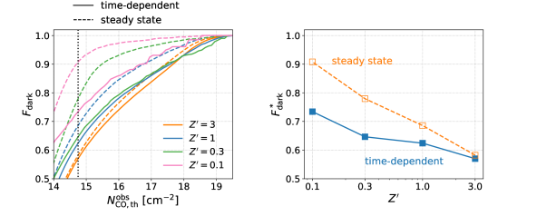
Figure 18: Left: The CO-dark H₂ mass fraction as a function of the threshold observed CO column density $N^{\rm obs}_{\rm CO,th}$ at different metallicities. The time-dependent H₂ model is shown in solid lines while the steady-state H₂ model is in dashed lines. The vertical black dotted line highlights $N^{\rm obs}_{\rm CO,th}=6\times 10^{14}{\rm cm^{-3}}$. Right: The CO-dark H₂ mass fraction defined with $N^{\rm obs}_{\rm CO,th}=6\times 10^{14}{\rm cm^{-3}}$ as a function of $Z^{\prime}$. The steady-state model significantly over-predicts the CO-dark H₂ mass fraction at low $Z^{\prime}$.

Table 3: Time-averaged global properties. The chemical properties are from the time-dependent H₂ model.

$Z^{\prime}$	$M_{\rm gas}$	${\rm SFR}$	$F_{\rm 100}$	$F_{\rm H^{+}}$	$F_{\rm H}$	$F_{\rm H_{2}}$	$F_{\rm C^{+}}$	$F_{\rm C}$	$F_{\rm CO}$	$F_{\rm dark}$
3	$8.3\times 10^{6}$	2.4$\times 10^{-3}$	0.025	0.097	0.84	0.066	4.79$\times 10^{-3}$	2.26$\times 10^{-4}$	6.55$\times 10^{-5}$	0.57
1	$8.5\times 10^{6}$	2.6$\times 10^{-3}$	0.023	0.085	0.90	0.020	1.65$\times 10^{-3}$	2.25$\times 10^{-5}$	5.87$\times 10^{-6}$	0.62
0.3	$8.4\times 10^{6}$	3.8$\times 10^{-3}$	0.017	0.078	0.92	0.0051	4.99$\times 10^{-4}$	4.72$\times 10^{-6}$	5.41$\times 10^{-7}$	0.65
0.1	$8.6\times 10^{6}$	2.5$\times 10^{-3}$	0.013	0.074	0.92	0.0017	1.67$\times 10^{-4}$	7.87$\times 10^{-7}$	2.95$\times 10^{-8}$	0.73

Note. — (1) Normalized metallicity. (2) Total gas mass (including helium and metals) in units of ${\rm M_{\odot}}$. (3) Total star formation rate in units of ${\rm M_{\odot}\ yr^{-1}}$. (4) Mass fraction with $n>100\ {\rm cm^{-3}}$. (5)-(10): Mass fraction (relative to total hydrogen mass) of H⁺, H, H₂, C⁺, C and CO. (11) Mass fraction of the CO-dark H₂ gas with $N^{\rm obs}_{\rm CO,th}=6\times 10^{14}{\rm cm^{-3}}$.

Table 4: Time-averaged global chemical properties in the steady-state H₂ model.

$Z^{\prime}$	$F_{\rm H^{+}}$	$F_{\rm H}$	$F_{\rm H_{2}}$	$F_{\rm C^{+}}$	$F_{\rm C}$	$F_{\rm CO}$	$F_{\rm dark}$
3	0.096	0.78	0.12	4.78$\times 10^{-3}$	2.22$\times 10^{-4}$	8.25$\times 10^{-5}$	0.58
1	0.085	0.86	0.052	1.66$\times 10^{-3}$	2.14$\times 10^{-5}$	7.87$\times 10^{-6}$	0.69
0.3	0.078	0.89	0.033	5.00$\times 10^{-4}$	3.84$\times 10^{-6}$	8.01$\times 10^{-7}$	0.80
0.1	0.074	0.91	0.019	1.67$\times 10^{-4}$	5.20$\times 10^{-7}$	6.76$\times 10^{-8}$	0.91

Note. — (1) Normalized metallicity. (2)-(7): Mass fraction (relative to total hydrogen mass) of H⁺, H, H₂, C⁺, C and CO. (8) Mass fraction of the CO-dark H₂ gas with $N^{\rm obs}_{\rm CO,th}=6\times 10^{14}{\rm cm^{-3}}$.

The fact that the conversions for H/H₂ occur at lower volume and column densities than for C/CO leads to a natural outcome that CO does not trace H₂ perfectly, which is readily visualized in Fig. 6. The H₂ gas that does not show a detectable CO emission is called “CO-dark”, which by definition depends on the detection limit. However, since we do not perform radiative transfer to obtain the CO emission in this work, we instead use a threshold value of $N^{\rm obs}_{\rm CO}$ as a proxy of the detection limit. The left panel in Fig. 18 shows the cumulative H₂ mass fraction as a function of $N^{\rm obs}_{\rm CO}$ at different metallicities. Equivalently, this is showing the mass fraction of the CO-dark H₂ gas, $F_{\rm dark}$, as a function of the adopted threshold $N^{\rm obs}_{\rm CO,th}$. The time-dependent H₂ model is shown in solid lines while the steady-state H₂ chemistry is in dashed lines. The vertical black dotted line highlights our adopted threshold $N^{\rm obs}_{\rm CO,th}=6\times 10^{14}{\rm cm^{-2}}$. This value roughly corresponds to a CO(1-0) line intensity $W_{\rm CO}$ = 0.75 K km s^-1, which is the CO sensitivity limit for recent observations of nearby galaxies (Lang et al., 2020), assuming $T=$ 20 K, $n=10^{3}$ cm^-3 and a linewidth of 3 km s^-1.

Our steady-state model suggests that $F_{\rm dark}$ increases significantly as $Z^{\prime}$ decreases, which is consistent with the standard PDR theories (e.g. Madden et al., 1997; Bolatto et al., 1999; Wolfire et al., 2010). However, because of the time-dependent effect, the actual H/H₂ conversions occur gradually and gas becomes half-molecular at a much higher density or column density. Consequently, $F_{\rm dark}$ becomes progressively lower than the steady-state prediction as $Z^{\prime}$ decreases. To show the trend with $Z^{\prime}$ more explicitly, the right panel in Fig. 18 shows the CO-dark H₂ mass fraction defined with $N^{\rm obs}_{\rm CO,th}=6\times 10^{14}{\rm cm^{-3}}$ as a function of $Z^{\prime}$. The actual $F^{*}_{\rm dark}$ still increases inversely with $Z^{\prime}$ but not nearly as much as in the steady-state model, as the latter significantly overestimates H₂ in the diffuse medium.

4.9 Model limitations

Our model does not account for spatial variations of the FUV radiation, which can be much stronger than the background radiation field in the vicinity of young stars. Hu et al. (2017) adopted a tree-based treatment assuming optically thin conditions and found that the H₂ fraction in a dwarf galaxy decreases only by a factor of two when switching from a constant FUV model to a variable FUV model, as the majority of gas is still subject to a smoothly varied background radiation. However, the optically thin assumption is expected to break down when the gas surface density or metallicity is high. A full consideration requires radiative transfer which, if computationally feasible, would not only capture the FUV spatial variations but also more naturally account for shielding without the need of the column density-based approximation.

For simplicity, we have assumed that the dust-to-gas mass ratio (DGR) scales linearly with metallicity. However, observations have suggested a super-linear scaling at low metallicities (Rémy-Ruyer et al., 2014), which means that the time-dependent effect should be even stronger than what we have shown at a given metallicity. In addition, the thermal equilibrium state will also be modified as photoelectric heating weakens faster than metal line cooling with decreasing metallicity.

5 Discussion

5.1 Comparison with previous simulations

In this section, we compare our results with previous simulations in the literature. As resolved multi-phase ISM simulations at low metallicities are rare, we will focus on the solar-metallicity case which is most widely studied.

Smith et al. (2014) simulated a large patch of the Milky Way and found $F_{\rm dark}=46\%$ adopting $N^{\rm obs}_{\rm CO,th}=10^{16}\ {\rm cm^{-2}}$. If we adopt the same threshold, we find $F_{\rm dark}=78\%$ in the time-dependent case which is significantly higher. However, their simulations did not include gravity and stellar feedback, both of which are expected to change the dynamics of gas substantially. In addition, their simulation domain covers a galactocentric radius from 5 kpc to 10 kpc with a radial profile of gas surface density, and so the results may not be directly comparable. Finally, their adopted chemistry network (NL97) tends to over-produce CO as shown in Glover & Clark (2012b). More recently, Smith et al. (2020) adopted a similar setup but included gravity and supernova feedback. They found $F_{\rm H_{2}}=21.4\%$ in their feedback-dominated model, significantly higher than our $Z^{\prime}=1$ run where $F_{\rm H_{2}}=2.0\%$. This again might be simply due to their larger simulation domain (their “zoom-in” box is 3 kpc on a side and centered on the solar galactocentric radius), which include regions with higher gas surface density. The molecular fraction is expected to be rather sensitive to the total hydrogen surface density around $\Sigma_{\rm H,tot}=10\ {\rm M_{\odot}pc^{-2}}$ as this is the transition between the atomic-dominated and molecular-dominated regimes (Bigiel et al., 2008). In our case, $\Sigma_{\rm H,tot}\approx 5.8\ {\rm M_{\odot}pc^{-2}}$, so the ISM is expected to be dominated by atomic hydrogen.

Seifried et al. (2017) performed “zoom-in” simulations of two molecular clouds taken from the SILCC simulations. They found a CO-to-H₂ mass ratio of $1.8\times 10^{-4}$, which is encouragingly similar to our value ($3.6\times 10^{-4}$ for $Z^{\prime}=1$). However, we caution that their simulations are only run for a short amount of time (5 Myr) due to the nature of zoom-ins, while in our case the results are averaged over 450 Myr with a time interval of 5 Myr and so the gas cycles are fairly well-sampled. It is therefore unclear if the agreement is physical or coincidental. As a follow-up work, Seifried et al. (2020) found $F_{\rm dark}=15-65\%$ with a broad range of scatter. Our time-dependent model finds $F_{\rm dark}=62\%$, which is within their scatter but is on the high end. Again, the two results may not be directly comparable due to the differences in cloud sampling. In addition, they found the conversions of H/H₂ and C/CO occur at $A_{V}\sim 1$ and $A_{V}\sim 1.3$, respectively, both of which are slightly lower than our time-dependent model ($A_{V}=1.5$ for H/H₂ and $A_{V}=2.5$ for C/CO).

The fairest comparison we can make is with Gong et al. (2018), who post-processed the TIGRESS simulations with a very similar setup to ours. They reported time-averaged results over 60 Myr with a time interval of 5 Myr which roughly covers one gas cycle and found $F_{\rm H_{2}}=12\%$, significantly higher than our 2%. However, as the TIGRESS simulations do not include time-dependent chemistry, they had to evolve the H₂ abundance to steady state and so their results should be compared to our steady-state H₂ model where $F_{\rm H_{2}}=5.1\%$. In addition, their column densities for shielding are integrated over the entire simulation box using a six-ray algorithm and thus the shielding length is effectively 500 pc. This could account for another factor of two difference in $F_{\rm H_{2}}$ as we show in Appendix B.1. In fact, the steady-state H₂ abundance should be even more sensitive to $L_{\rm sh}$. In terms of CO, they found a total CO mass about four times higher than in our steady-state H₂ model, which seems too much to be accounted for by the difference in $L_{\rm sh}$. In fact, it is more likely to be explained by the difference in the effective visual extinction where the C/CO conversions occur, which in their case is around 1.3, slightly lower than our 2.2, presumably due to the difference in the H₂ column densities. As $A^{\rm eff}_{V}\propto n^{0.3}$ at $Z^{\prime}=1$, a small difference in $A^{\rm eff}_{V}$ implies a notable difference in the conversion density, which is reflected in their CO density histogram which peaks at a much lower density $n\sim 300\ {\rm cm}^{-3}$. For the CO-dark H₂ mass fraction, they used an intensity-based threshold $W_{\rm CO}$ = 0.75 K km s^-1 and found $F_{\rm dark}=56\%$, while in their more recent model in Gong et al. (2020) (also with steady-state chemistry), they found $F_{\rm dark}=61\%$. Our adopted threshold of $N^{\rm obs}_{\rm CO,th}=6\times 10^{14}\ {\rm cm^{-2}}$ is designed to match their threshold. We find a slightly higher value of 69% in our steady-state model. Coincidentally, our time-dependent model shows $F_{\rm dark}=62\%$ which is in better agreement with their results.

5.2 Observational implications

Our results suggest that steady-state chemistry can significantly overestimate $F_{\rm dark}$ at low metallicities, as the dynamical time is too short for H₂ to reach its steady-state abundance. Recently, Madden et al. (2020) investigated nearby dwarf galaxies using spectral synthesis models and concluded that $F_{\rm dark}$ ranges from 70% to 100%. We caution that these numbers should be viewed as an upper limit as steady-state chemistry is used. Admittedly, our simulations do not cover the parameter space of different gas and stellar surface densities. In low-surface density environments such as dwarf galaxies, the SFR surface density is lower which may result in a less violent ISM and a longer dynamical time. In such cases, the time-dependent effect would be less pronounced. We therefore expect that the actual $F_{\rm dark}$ in dwarf galaxies should be somewhere between our time-dependent and steady-state models as shown in Fig. 18, which warrants future investigations.

We stress that the lower $F_{\rm dark}$ we find at low $Z^{\prime}$ is mainly due to the significantly under-abundant H₂. CO emission, in the absolute sense, does not becomes brighter by the time-dependent effect. If anything, it should become slightly fainter. CO traces H₂ better in the time-dependent model simply because there is little H₂ in the diffuse cold gas. This raises the question whether it is useful to obtain an accurate total H₂ mass given that the correlation between H₂ and star formation breaks down at low $Z^{\prime}$.

6 Summary

We conduct high-resolution (particle mass of $1\ {\rm M_{\odot}}$, effective spatial resolution $\sim$ 0.2 pc) hydrodynamical simulations to study the metallicity dependence of H₂ and CO in a multi-phase, self-regulating ISM, covering a wide range of metallicities $0.1<Z^{\prime}<3$. We adopt a hybrid technique where we use a simple chemistry network to follow H₂ and H⁺ on-the-fly and then post-process other species with an accurate chemistry network. This allows us to simultaneously capture the time-dependent effect of H₂ and follow all the relevant CO formation and destruction channels. Our post-processing chemistry network includes 31 species and 286 reactions which accurately reproduces the C⁺/C/CO transitions as in classical PDR calculations (Fig. 1). Our chemistry code for post-processing is publicly available and is archived in Zenodo (Hu, 2021). Our main findings can be summarized as follows.

1. The ratios $M_{\rm H_{2}}/M_{\rm C^{+}}$ and $M_{\rm H_{2}}/M_{\rm C}$ both show a weaker dependence on $Z^{\prime}$ than $M_{\rm H_{2}}/M_{\rm CO}$, which potentially indicates that C⁺ and C could be viable alternative tracers for H₂ at low $Z^{\prime}$ in terms of mass budget. At low $Z^{\prime}$, the steady-state model significantly overestimates $M_{\rm H_{2}}$ but not $M_{\rm CO}$ (Fig. 17). As such, the CO-dark H₂ mass fraction is significantly lower than what a steady-state model predicts at low $Z^{\prime}$ (Fig. 18). The global properties are summarized in Tables 3 and 4.

2. The averaged SFR is insensitive to $Z^{\prime}$, while the temporal fluctuation of SFR increases inversely with $Z^{\prime}$ (Fig. 2). The median temperature as a function of density is insensitive to $Z^{\prime}$, as the dominant cooling and heating processes both scale linearly with $Z^{\prime}$ and thus they cancel out. At lower $Z^{\prime}$, the median temperature in the cold gas is slightly higher (Figs. 7).

3. The typical cloud size roughly follows the thermal Jeans length and is thus insensitive to $Z^{\prime}$. This leads to a correlation between $n$ and $N^{\rm eff}$. As $Z^{\prime}$ increases, dust extinction kicks in at a lower column density, leading to a slightly flatter relationship from $N^{\rm eff}\propto n^{0.39}$ at $Z^{\prime}=0.1$ to $N^{\rm eff}\propto n^{0.3}$ at $Z^{\prime}=3$. (Fig. 9 and Eq. 14).

4. Using the correlation between $n$ and $N^{\rm eff}$, we construct 1D effective density profiles of typical clouds and conduct PDR calculations. The results successfully capture the time-averaged chemical distributions in the actual simulations (Fig. 11).

5. As $Z^{\prime}$ decreases, H₂ becomes progressively under-abundant compared to its steady-state counterpart (which serves as an upper limit) as it is mainly limited by the dynamical time rather than by photodissociation. The H₂ abundance follows a shallow profile which can be well-described by an analytic expression with a $Z^{\prime}$-indepedent dynamical time (Eq. 15) up to the photodissociation surface where it is sharply truncated. In contrast, the CO profile is sharp and controlled by photodissociation as CO forms rapidly and has reached steady state. The under-abundant H₂ has little impact on the C⁺/C/CO conversions (Figs. 10 and 12). The conversion densities, column densities and visual extinctions are summarized in Tables 1 and 2.

6. The shallow H₂ profile leads to a significant contribution of gas with low H₂ abundance to the total H₂ reservoir. In addition, the density where most H₂ can be found is significantly lower than the H₂ conversion density (Figs. 13 and 14).

7. The time-dependent effect helps explain the observed relationship between $N^{\rm obs}_{\rm H_{2}}$ and $N^{\rm obs}_{\rm CO}$ for the Galactic clouds without resorting to non-thermal velocity distributions for the reaction C⁺ + H₂ $\rightarrow$ CH⁺ + H (Fig. 15).

8. For a given $N^{\rm obs}_{\rm H_{2}}$, our fiducial model reproduces the observed $N^{\rm obs}_{\rm C^{+}}$ and $N^{\rm obs}_{\rm CO}$ but significantly over-produces $N^{\rm obs}_{\rm C}$ in the Galactic clouds. Only when we artificially switch off recombination on grains can we reproduce all the three quantities simultaneously (Fig. 16).

Appendix A Chemical timescales

In this section, we investigate the timescales for C⁺, C and CO to reach steady state.

For the C⁺/C transition, the relevant timescale is C⁺ recombination $t_{\rm rec,C}$. To measure $t_{\rm rec,C}$, we run the chemistry network in a one-zone setup where $T=30$ K, $\zeta_{\rm CR}=10^{-16}{\rm s^{-1}}$, $I_{\rm UV}=0$ and $n$ systematically varies from 10 to $10^{4}\ {\rm cm^{-3}}$. We adopt $I_{\rm UV}=0$ such that C⁺ will recombine even at low densities. Adopting a nonzero $I_{\rm UV}$ does not change $t_{\rm rec,C}$ significantly. All carbon is initially in the form of C⁺ ($x_{\rm C^{+}}/x_{\rm C,0}=1$) which gradually recombines as time evolves. We record $t_{\rm rec,C}$ as the time where $x_{\rm C^{+}}/x_{\rm C,0}<\exp(-1)$ first occurs. Fig. 19 shows $t_{\rm rec,C}$ as a function of $n$. The dashed line shows the dynamical time $t_{\rm dyn}$ in our simulations which is insensitive to $Z^{\prime}$ (see Sec. 4.4). $t_{\rm rec,C}$ scales roughly as $(nZ^{\prime})^{-1}$, as expected for two-body reactions. In all cases, $t_{\rm rec,C}$ is orders of magnitude shorter than $t_{\rm dyn}$, justifying our steady-state assumption.

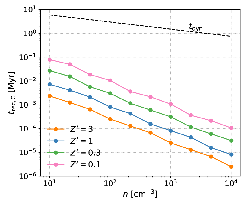
Figure 19: The C⁺ recombination time $t_{\rm rec,C}$ as a function of $n$ at different metallicities. The dashed line shows the dynamical time $t_{\rm dyn}$ in our simulations. In all cases, $t_{\rm rec,C}$ is orders of magnitude shorter than $t_{\rm dyn}$, justifying our steady-state assumption.

For the C/CO transition, the relevant timescale is CO formation $t_{\rm form,CO}$. We are interested in the case where gas is already fully molecular ($2x_{\rm H_{2}}\lesssim 1$). The left panel in Fig. 20 shows $t_{\rm form,CO}$ as a function of $n$, with $T=30$ K, $\zeta_{\rm CR}=10^{-16}{\rm s^{-1}}$ and $I_{\rm UV}=0$. All carbon is initially in the form of C⁺, while hydrogen is 90% in H₂ ($2x_{\rm H_{2}}=0.9$) and 10% in atomic H. The dashed line shows the dynamical time $t_{\rm dyn}$ in our simulations while the dotted line is the H₂ formation time $t_{\rm form,H_{2}}$ at $Z^{\prime}=1$ (see Eq. 11). We record $t_{\rm form,CO}$ as the time where $x_{\rm CO}/x_{\rm C,0}>1-\exp(-1)$ (or, equivalently, $x_{\rm C}/x_{\rm C,0}<\exp(-1)$) first occurs. CO forms mainly via two routes: the OH-channel and CH-channel. Both routes are facilitated by cosmic-ray ionization which produces ions such as H${}^{+}_{3}$ and initiates subsequent chemistry. As cosmic-ray ionization does not depend explicitly on either $n$ or $Z^{\prime}$, $t_{\rm form,CO}$ shows a much weaker dependence on both $n$ and $Z^{\prime}$, as opposed to $t_{\rm form,H_{2}}$ which scales as $(nZ^{\prime})^{-1}$. Instead, $t_{\rm form,CO}$ depends primarily on $\zeta_{\rm CR}$. For $\zeta_{\rm CR}=10^{-16}{\rm s^{-1}}$ (the averaged value in our simulations), $t_{\rm form,CO}$ is significantly lower than $t_{\rm dyn}$ at all densities and metallicities, justifying our steady-state assumption. If we adopt $\zeta_{\rm CR}=10^{-17}{\rm s^{-1}}$ (middle panel of Fig. 20), $t_{\rm form,CO}$ increases by a factor of 3 to 5 and becomes comparable to $t_{\rm dyn}$. In this case, the steady-state assumption is only marginally justified. Finally, if we adopt $\zeta_{\rm CR}=0$ (right panel of Fig. 20), $t_{\rm form,CO}$ becomes orders of magnitude longer especially at low $n$, and it scales roughly with $(nZ^{\prime})^{-1}$ as it is dictated by two-body reactions. Our $\zeta_{\rm CR}=0$ case for $Z^{\prime}=1$ agrees well with the timescale estimated by Joshi et al. (2019) ($t_{\rm form,CO}=10^{3.7}(n/({\rm cm^{-3}}))^{-1}$ Myr, their Eq. 38). This makes sense as they adopted the chemistry network of NL97, which ignores the effect of cosmic ray ionization in CO formation, leading to a significantly overestimated $t_{\rm form,CO}$ that scales with $n^{-1}$.

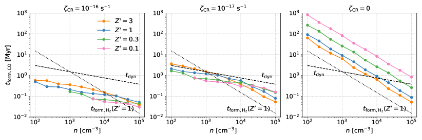
Figure 20: The CO formation time $t_{\rm form,CO}$ as a function of $n$ at different metallicities. The dashed line shows the dynamical time $t_{\rm dyn}$ in our simulations while the dotted line shows the CO formation time $t_{\rm form,H_{2}}$ at $Z^{\prime}=1$. Hydrogen is initially 90% in H₂ ($2x_{\rm H_{2}}=0.9$). For $\zeta_{\rm CR}=10^{-16}{\rm s^{-1}}$ (the averaged value in our simulations), $t_{\rm form,CO}$ is significantly lower than $t_{\rm dyn}$ at all densities and metallicities, justifying our steady-state assumption.

Appendix B Model robustness

B.1 Shielding length

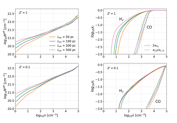
Figure 21: Effective column density (left) and normalized chemical abundances (right) as a function of density for $L_{\rm sh}=$ 50 (orange), 100 (blue), 200 (green) and 500 pc (pink) with $Z^{\prime}=1$ (top) and $Z^{\prime}=0.1$ (bottom). The solid and dashed lines show the normalized abundances of H₂ and CO, respectively. From $L_{\rm sh}=$ 50 pc to $L_{\rm sh}=$ 500 pc, $M_{\rm H_{2}}$ and $M_{\rm CO}$ increase, respectively, by a factor of 2.4 and 1.6 at $Z^{\prime}=1$, and by a factor of 1.16 and 1.08 at $Z^{\prime}=0.1$.

In this section, we investigate how the choice of $L_{\rm sh}$ affects the molecular abundance. Fig. 21 shows $N^{\rm eff}$ (left) and normalized chemical abundances (right) as a function of $n$ for $L_{\rm sh}=$ 50 (orange), 100 (blue), 200 (green) and 500 pc (pink) with $Z^{\prime}=1$ (top) and $Z^{\prime}=0.1$ (bottom). The solid and dashed lines show the normalized abundances of H₂ and CO, respectively. For computational efficiency, these simulations were run with $m_{\rm g}=3\ {\rm M_{\odot}}$ (instead of $m_{\rm g}=1\ {\rm M_{\odot}}$ as in our default runs).

In general, a larger $L_{\rm sh}$ leads to a higher $N^{\rm eff}$. The largest difference is found in the diffuse medium, within a factor of three at $n\sim 10\ {\rm cm^{-3}}$ between the two extreme cases. In dense clouds, the major contribution to shielding is from gas in the vicinity rather than from the diffuse volume-filling background, and thus $N^{\rm eff}$ is insensitive to $L_{\rm sh}$ at high $n$. As the H₂ profile is mainly controlled by the dynamical time, the conversion density for H₂ (where $x_{\rm H}=x_{\rm H_{2}}$) is insensitive to $L_{\rm sh}$. The effect of $L_{\rm sh}$ only appears near the photodissociation front in the $Z^{\prime}=1$ run, where a larger $L_{\rm sh}$ implies more shielding at a given density, shifting the photodissociation front towards at a lower density. At $Z^{\prime}=0.1$, the effect of $L_{\rm sh}$ becomes even weaker as the H₂ profile is mainly governed by the dynamical time. In contrast, the C/CO conversions are controlled by photodissociation which is shifted towards a lower density or column density as $L_{\rm sh}$ increases. Fortunately, this occurs at high enough column densities such that the corresponding density is similar, and thus $M_{\rm CO}$ is also insensitive to $L_{\rm sh}$. From $L_{\rm sh}=$ 50 pc to $L_{\rm sh}=$ 500 pc, $M_{\rm H_{2}}$ and $M_{\rm CO}$ increase, respectively, by a factor of 2.4 and 1.6 at $Z^{\prime}=1$, and by a factor of 1.16 and 1.08 at $Z^{\prime}=0.1$.

B.2 Recombination on grains

Recombination on grains can be more efficient than radiative recombination and becomes the dominant destruction process for positive ions in some circumstances (Weisheit & Upham, 1978; Draine & Sutin, 1987; Lepp et al., 1988; Weingartner & Draine, 2001). Gong et al. (2017) found that including recombinations on grains is crucial in order to obtain the correct CO abundance in their PDR calculations. Fig. 22 shows the normalized abundances of C⁺ (blue), C (orange) and CO (green) as a function of density for $Z^{\prime}=$ 3, 1, 0.3 and 0.1 from top to bottom. The solid and dashed lines represent models with and without recombinations on grains. Recombination on grains shifts the conversions of both C⁺/C and C/CO to lower densities, but the effect is significantly more pronounced in the former. For $Z^{\prime}=$ 3, 1, 0.3 and 0.1, including recombination on grains increases $M_{\rm C}$ by a factor of 3.9, 4.3, 5.9 and 4.5, while increases $M_{\rm CO}$ by a factor of 2, 1.6, 1.2 and 1.1, respectively. Contrary to Gong et al. (2017), we find that $M_{\rm CO}$ is only marginally affected by recombination on grains as CO formation occurs at higher densities in our simulations. Indeed, we have confirmed that in one-zone PDR calculations, recombination on grains makes a increasingly larger difference on the CO abundance with decreasing density, as also seen in Gong et al. (2017).

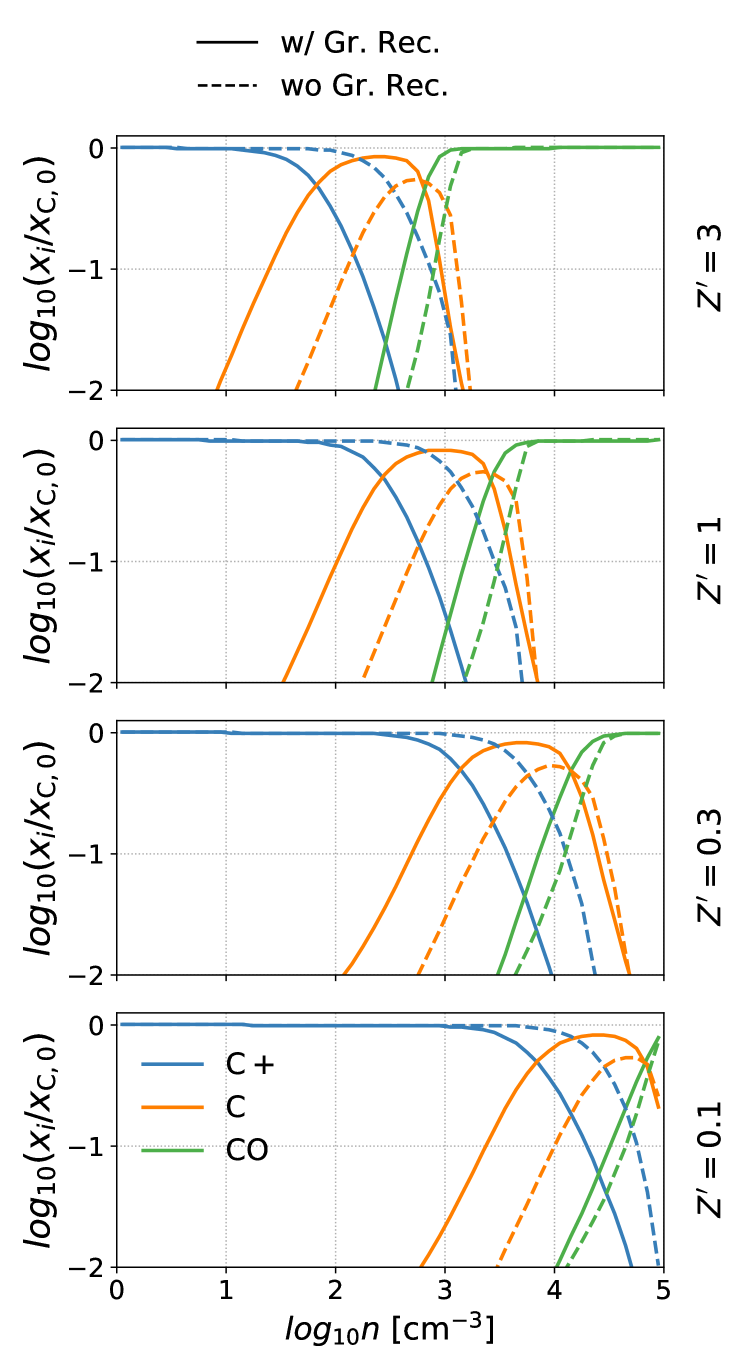
Figure 22: Normalized abundances of C⁺ (blue), C (orange) and CO (green) as a function of density for $Z^{\prime}=$ 3, 1, 0.3 and 0.1 from top to bottom. The solid and dashed lines represent models with and without recombinations on grains. For $Z^{\prime}=$ 3, 1, 0.3 and 0.1, including recombination on grains increases $M_{\rm C}$ by a factor of 3.9, 4.3, 5.9 and 4.5, while increases $M_{\rm CO}$ by a factor of 2, 1.6, 1.2 and 1.1, respectively.

Appendix C Numerical robustness

C.1 Convergence study

Fig. 23 shows the time-averaged density histogram with five different mass resolutions $m_{\rm g}$ for $Z^{\prime}=$ 3, 1, 0.3 and 0.1 from top to bottom. The high density tail is gradually converged as $m_{\rm g}$ decreases. However, the convergence occurs faster at lower $Z^{\prime}$. This is related to the difference in the star formation density threshold (see Fig. 7), which is generally higher at lower $Z^{\prime}$ due to a higher temperature of clouds. At high $Z^{\prime}$, star formation occurs at lower densities which efficiently stops the gravitational collapse and removes the high-density gas.

In terms of the global properties, Fig. 24 shows the time-averaged SFR (top), $M_{\rm H_{2}}$ (middle) and $M_{\rm CO}$ (bottom) as a function of $m_{\rm g}$, normalized to the results in the highest resolution ($m_{\rm g}=1\ {\rm M_{\odot}}$). Among the three quantities, the SFR is the easiest to converge. Even at $m_{\rm g}=1\ {\rm M_{\odot}}$, the SFR is converged within a factor of 50% and show a diverging trend with resolution. On the other hand, both $M_{\rm H_{2}}$ and $M_{\rm CO}$ show a clear trend of diverging (underestimation) as $m_{\rm g}$ increases, with $M_{\rm CO}$ diverging faster. This is expected as CO forms at higher densities than H₂ which requires a higher resolution to resolve. Interestingly, the $Z^{\prime}=0.1$ run performs as well as the $Z^{\prime}=3$ run in terms of convergence, with both $M_{\rm H_{2}}$ and $M_{\rm CO}$ converge within 10% at $m_{\rm g}=3\ {\rm M_{\odot}}$. This is because while both H₂ and CO form at higher densities at lower $Z^{\prime}$, its density histogram is also converged up to a higher density due to a higher SFR density threshold. In contrast, the $Z^{\prime}=1$ and $Z^{\prime}=0.3$ runs have $M_{\rm H_{2}}$ and $M_{\rm CO}$ converged within, respectively, around 20% and 50% at $m_{\rm g}=3\ {\rm M_{\odot}}$, which is slightly worse than the other two runs. This demonstrates that there is no universal resolution requirement for the convergence of molecular abundances, which occurs once the density histogram converges up to the conversion densities for H/H₂ and C/CO.

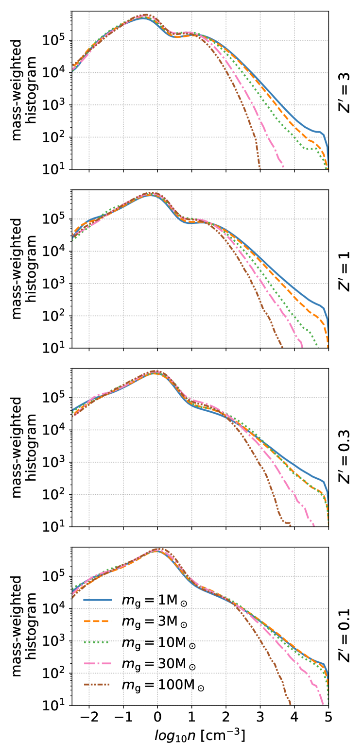
Figure 23: Time-averaged density histogram with five different mass resolutions for $Z^{\prime}=$ 3, 1, 0.3 and 0.1 from top to bottom.

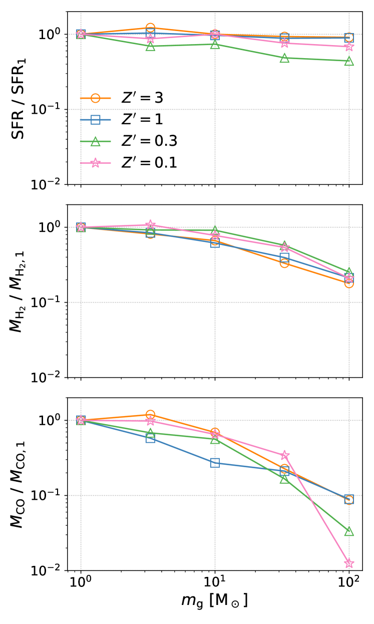
Figure 24: Time-averaged SFR (top), total H₂ mass (middle) and total CO mass (bottom) as a function of $m_{\rm g}$, normalized to the results in the highest resolution ($m_{\rm g}=1\ {\rm M_{\odot}}$).

C.2 Instantaneous star formation threshold

In this section, we demonstrate the effect of instantaneous star formation density threshold $n_{\rm isf}$ (see Sec. 2.3) by running two additional simulations with $n_{\rm isf}=10^{7}\ {\rm cm^{-3}}$. Fig. 25 shows the density histogram at $Z^{\prime}=0.3$ (green) and $Z^{\prime}=0.1$ (pink). The solid and dashed lines represent $n_{\rm isf}=10^{5}\ {\rm cm^{-3}}$ and $n_{\rm isf}=10^{7}\ {\rm cm^{-3}}$, respectively.

With $n_{\rm isf}=10^{7}\ {\rm cm^{-3}}$, the gas collapses way beyond the Jeans mass threshold, which corresponds to $n\sim 3\times 10^{4}\ {\rm cm^{-3}}$ (see Fig. 7), and piles up at high densities. As such, the histogram becomes flat above $10^{5}\ {\rm cm^{-3}}$. This leads to $M_{\rm CO}$ increasing by a factor of 1.2 and 4.0 in the $Z^{\prime}=0.3$ and $Z^{\prime}=0.1$ runs, respectively. The effect is less significant at higher $Z^{\prime}$ as the C/CO conversions occur at lower densities where the density distribution is still unaffected. Likewise, as H₂ forms at much lower densities, $M_{\rm H_{2}}$ is increased by a factor of 1.05 for $Z^{\prime}=0.3$ and is even decreased by a factor of 0.96 for $Z^{\prime}=0.1$. Therefore, although our choice of $n_{\rm isf}$ is numerics-motivated and somewhat arbitrary, it only has a significant effect on $M_{\rm CO}$ at $Z^{\prime}=0.1$. Moreover, we argue that the flat density distribution with $n_{\rm isf}=10^{7}\ {\rm cm^{-3}}$ is unrealistic as self-gravitating clouds are expected to follow a declining power-law distribution.

The stochastic star formation recipe we adopt has been the standard approach in cosmological simulations. Adding an instantaneous density threshold in the stochastic method has been proposed in Lahén et al. (2019) with $4{\rm M_{\odot}}$-resolution. Moreover, the “sink-particle” method, which is commonly used in cloud-scale simulations, is also an instantaneous star formation model. It therefore appears that removing gravitationally unresolved gas instantaneously (rather than waiting for a few free-fall times) is numerically beneficial as one goes from cosmological scales to ISM scales.

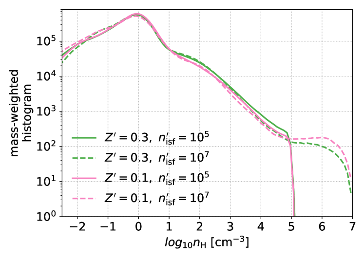
Figure 25: Density histogram at $Z^{\prime}=0.3$ (green) and $Z^{\prime}=0.1$ (pink). The solid and dashed lines represent $n_{\rm isf}=10^{5}\ {\rm cm^{-3}}$ and $n_{\rm isf}=10^{7}\ {\rm cm^{-3}}$, respectively.

C.3 Chemistry iteration

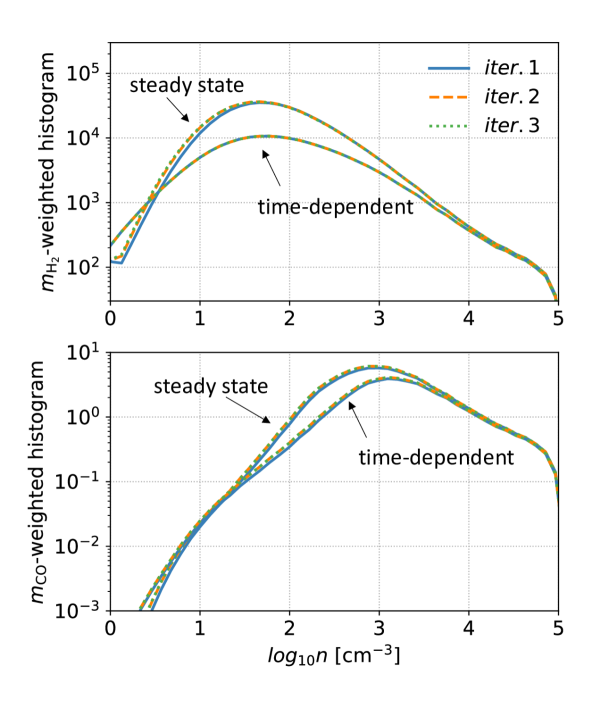
Figure 26: Time-averaged density histograms of H₂ (top) and CO (bottom) for the $Z^{\prime}=1$ case for each iteration (iter. 1, 2 and 3) when solving the post-processing chemistry network. Both $x_{\rm H_{2}}$ and $x_{\rm CO}$ converge rapidly.

As discussed in Sec. 3.3, solving the chemistry network in post-processing requires iterations as shielding from gas depends on the nonlocal quantities $x_{\rm H_{2}}$ and $x_{\rm CO}$. In Fig. 26, we show the time-averaged density histograms of H₂ and CO for the $Z^{\prime}=1$ case for each iteration. For the time-dependent case, $x_{\rm H_{2}}$ is treated as given and therefore remains fixed during the iterations. $x_{\rm CO}$ converges rapidly ($M_{\rm CO}/{\rm M_{\odot}}$ = 33.7, 35.4 and 35.4 from the first to third iteration) as dust shielding and H₂ shielding for CO are already known. The difference in $x_{\rm CO}$ between the first and the final iterations reflects the effect of CO self-shielding, which only increases $M_{\rm CO}$ by 5%. For the steady-state case, both $x_{\rm H_{2}}$ and $x_{\rm CO}$ require iterations. We use the time-dependent $x_{\rm H_{2}}$ as the initial guess in the first iteration which facilitates the convergence. From the first to third iteration, $M_{\rm H_{2}}/(10^{5}{\rm M_{\odot}})$ = 2.98, 3.15, 3.14 while $M_{\rm CO}/{\rm M_{\odot}}$ = 44.7, 47.5 and 47.5, respectively.

References

- Andreani et al. (2018) Andreani, P., Retana-Montenegro, E., Zhang, Z.-Y., et al. 2018, A&A, 615, A142, doi: 10.1051/0004-6361/201732560
- Bialy (2020) Bialy, S. 2020, ApJ, 903, 62, doi: 10.3847/1538-4357/abb804
- Bialy & Sternberg (2019) Bialy, S., & Sternberg, A. 2019, ApJ, 881, 160, doi: 10.3847/1538-4357/ab2fd1
- Bigiel et al. (2008) Bigiel, F., Leroy, A., Walter, F., et al. 2008, AJ, 136, 2846, doi: 10.1088/0004-6256/136/6/2846
- Bisbas et al. (2019) Bisbas, T. G., Schruba, A., & van Dishoeck, E. F. 2019, MNRAS, 485, 3097, doi: 10.1093/mnras/stz405
- Bisbas et al. (2017) Bisbas, T. G., van Dishoeck, E. F., Papadopoulos, P. P., et al. 2017, ApJ, 839, 90, doi: 10.3847/1538-4357/aa696d
- Black & van Dishoeck (1987) Black, J. H., & van Dishoeck, E. F. 1987, ApJ, 322, 412, doi: 10.1086/165740
- Boger & Sternberg (2005) Boger, G. I., & Sternberg, A. 2005, ApJ, 632, 302, doi: 10.1086/432864
- Bolatto et al. (1999) Bolatto, A. D., Jackson, J. M., & Ingalls, J. G. 1999, ApJ, 513, 275, doi: 10.1086/306849
- Bolatto et al. (2013) Bolatto, A. D., Wolfire, M., & Leroy, A. K. 2013, ARA&A, 51, 207, doi: 10.1146/annurev-astro-082812-140944
- Bourne et al. (2019) Bourne, N., Dunlop, J. S., Simpson, J. M., et al. 2019, MNRAS, 482, 3135, doi: 10.1093/mnras/sty2773
- Burgh et al. (2010) Burgh, E. B., France, K., & Jenkins, E. B. 2010, ApJ, 708, 334, doi: 10.1088/0004-637X/708/1/334
- Cardelli et al. (1994) Cardelli, J. A., Sofia, U. J., Savage, B. D., Keenan, F. P., & Dufton, P. L. 1994, ApJ, 420, L29, doi: 10.1086/187155
- Clark et al. (2012) Clark, P. C., Glover, S. C. O., & Klessen, R. S. 2012, MNRAS, 420, 745, doi: 10.1111/j.1365-2966.2011.20087.x
- Cormier et al. (2014) Cormier, D., Madden, S. C., Lebouteiller, V., et al. 2014, A&A, 564, A121, doi: 10.1051/0004-6361/201322096
- Dalgarno & Black (1976) Dalgarno, A., & Black, J. H. 1976, Reports on Progress in Physics, 39, 573, doi: 10.1088/0034-4885/39/6/002
- De Looze et al. (2011) De Looze, I., Baes, M., Bendo, G. J., Cortese, L., & Fritz, J. 2011, MNRAS, 416, 2712, doi: 10.1111/j.1365-2966.2011.19223.x
- Dessauges-Zavadsky et al. (2020) Dessauges-Zavadsky, M., Ginolfi, M., Pozzi, F., et al. 2020, A&A, 643, A5, doi: 10.1051/0004-6361/202038231
- Draine (1978) Draine, B. T. 1978, ApJS, 36, 595, doi: 10.1086/190513
- Draine & Bertoldi (1996) Draine, B. T., & Bertoldi, F. 1996, ApJ, 468, 269, doi: 10.1086/177689
- Draine & Sutin (1987) Draine, B. T., & Sutin, B. 1987, ApJ, 320, 803, doi: 10.1086/165596
- Duarte-Cabral et al. (2015) Duarte-Cabral, A., Acreman, D. M., Dobbs, C. L., et al. 2015, MNRAS, 447, 2144, doi: 10.1093/mnras/stu2586
- Ekström et al. (2012) Ekström, S., Georgy, C., Eggenberger, P., et al. 2012, A&A, 537, A146, doi: 10.1051/0004-6361/201117751
- Emerick et al. (2019) Emerick, A., Bryan, G. L., & Mac Low, M.-M. 2019, MNRAS, 482, 1304, doi: 10.1093/mnras/sty2689
- Evans et al. (2009) Evans, Neal J., I., Dunham, M. M., Jørgensen, J. K., et al. 2009, ApJS, 181, 321, doi: 10.1088/0067-0049/181/2/321
- Federman et al. (1996) Federman, S. R., Rawlings, J. M. C., Taylor, S. D., & Williams, D. A. 1996, MNRAS, 279, L41, doi: 10.1093/mnras/279.3.L41
- Feldmann et al. (2012) Feldmann, R., Gnedin, N. Y., & Kravtsov, A. V. 2012, ApJ, 747, 124, doi: 10.1088/0004-637X/747/2/124
- Field et al. (1969) Field, G. B., Goldsmith, D. W., & Habing, H. J. 1969, ApJ, 155, L149, doi: 10.1086/180324
- Fuchs et al. (2009) Fuchs, B., Jahreiß, H., & Flynn, C. 2009, AJ, 137, 266, doi: 10.1088/0004-6256/137/1/266
- Gaburov & Nitadori (2011) Gaburov, E., & Nitadori, K. 2011, MNRAS, 414, 129, doi: 10.1111/j.1365-2966.2011.18313.x
- Gatto et al. (2015) Gatto, A., Walch, S., Low, M.-M. M., et al. 2015, MNRAS, 449, 1057, doi: 10.1093/mnras/stv324
- Gatto et al. (2017) Gatto, A., Walch, S., Naab, T., et al. 2017, MNRAS, 466, 1903, doi: 10.1093/mnras/stw3209
- Genzel et al. (2010) Genzel, R., Tacconi, L. J., Gracia-Carpio, J., et al. 2010, MNRAS, 407, 2091, doi: 10.1111/j.1365-2966.2010.16969.x
- Girichidis et al. (2016) Girichidis, P., Walch, S., Naab, T., et al. 2016, MNRAS, 456, 3432, doi: 10.1093/mnras/stv2742
- Glover & Clark (2012a) Glover, S. C. O., & Clark, P. C. 2012a, MNRAS, 426, 377, doi: 10.1111/j.1365-2966.2012.21737.x
- Glover & Clark (2012b) —. 2012b, MNRAS, 421, 116, doi: 10.1111/j.1365-2966.2011.20260.x
- Glover & Clark (2012c) —. 2012c, MNRAS, 421, 9, doi: 10.1111/j.1365-2966.2011.19648.x
- Glover et al. (2010) Glover, S. C. O., Federrath, C., Mac Low, M.-M., & Klessen, R. S. 2010, MNRAS, 404, 2, doi: 10.1111/j.1365-2966.2009.15718.x
- Glover & Mac Low (2007) Glover, S. C. O., & Mac Low, M.-M. 2007, ApJS, 169, 239, doi: 10.1086/512238
- Glover & Mac Low (2011) —. 2011, MNRAS, 412, 337, doi: 10.1111/j.1365-2966.2010.17907.x
- Gong et al. (2018) Gong, M., Ostriker, E. C., & Kim, C.-G. 2018, ApJ, 858, 16, doi: 10.3847/1538-4357/aab9af
- Gong et al. (2020) Gong, M., Ostriker, E. C., Kim, C.-G., & Kim, J.-G. 2020, ApJ, 903, 142, doi: 10.3847/1538-4357/abbdab
- Gong et al. (2017) Gong, M., Ostriker, E. C., & Wolfire, M. G. 2017, ApJ, 843, 38, doi: 10.3847/1538-4357/aa7561
- Górski & Hivon (2011) Górski, K. M., & Hivon, E. 2011, HEALPix: Hierarchical Equal Area isoLatitude Pixelization of a sphere, Astrophysics Source Code Library. http://ascl.net/1107.018
- Haardt & Madau (2012) Haardt, F., & Madau, P. 2012, ApJ, 746, 125, doi: 10.1088/0004-637X/746/2/125
- Heays et al. (2017) Heays, A. N., Bosman, A. D., & van Dishoeck, E. F. 2017, A&A, 602, A105, doi: 10.1051/0004-6361/201628742
- Hollenbach & McKee (1979) Hollenbach, D., & McKee, C. F. 1979, ApJS, 41, 555, doi: 10.1086/190631
- Hopkins (2015) Hopkins, P. F. 2015, MNRAS, 450, 53, doi: 10.1093/mnras/stv195
- Hopkins et al. (2018) Hopkins, P. F., Wetzel, A., Kereš, D., et al. 2018, MNRAS, 480, 800, doi: 10.1093/mnras/sty1690
- Hu (2019) Hu, C.-Y. 2019, MNRAS, 483, 3363, doi: 10.1093/mnras/sty3252
- Hu (2021) Hu, C.-Y. 2021, AstroChemistry, Zenodo, doi: 10.5281/zenodo.4775808
- Hu et al. (2017) Hu, C.-Y., Naab, T., Glover, S. C. O., Walch, S., & Clark, P. C. 2017, MNRAS, 471, 2151, doi: 10.1093/mnras/stx1773
- Hu et al. (2016) Hu, C.-Y., Naab, T., Walch, S., Glover, S. C. O., & Clark, P. C. 2016, MNRAS, 458, 3528, doi: 10.1093/mnras/stw544
- Hunt et al. (2015) Hunt, L. K., García-Burillo, S., Casasola, V., et al. 2015, A&A, 583, A114, doi: 10.1051/0004-6361/201526553
- Indriolo & McCall (2012) Indriolo, N., & McCall, B. J. 2012, ApJ, 745, 91, doi: 10.1088/0004-637X/745/1/91
- Indriolo et al. (2015) Indriolo, N., Neufeld, D. A., Gerin, M., et al. 2015, ApJ, 800, 40, doi: 10.1088/0004-637X/800/1/40
- Jiao et al. (2019) Jiao, Q., Zhao, Y., Lu, N., et al. 2019, ApJ, 880, 133, doi: 10.3847/1538-4357/ab29ed
- Joshi et al. (2019) Joshi, P. R., Walch, S., Seifried, D., et al. 2019, MNRAS, 484, 1735, doi: 10.1093/mnras/stz052
- Kaufman et al. (1999) Kaufman, M. J., Wolfire, M. G., Hollenbach, D. J., & Luhman, M. L. 1999, ApJ, 527, 795, doi: 10.1086/308102
- Kim & Ostriker (2017) Kim, C.-G., & Ostriker, E. C. 2017, ApJ, 846, 133, doi: 10.3847/1538-4357/aa8599
- Kim et al. (2020) Kim, C.-G., Ostriker, E. C., Somerville, R. S., et al. 2020, ApJ, 900, 61, doi: 10.3847/1538-4357/aba962
- Kroupa (2001) Kroupa, P. 2001, MNRAS, 322, 231, doi: 10.1046/j.1365-8711.2001.04022.x
- Krumholz (2012) Krumholz, M. R. 2012, ApJ, 759, 9, doi: 10.1088/0004-637X/759/1/9
- Lada & Lada (2003) Lada, C. J., & Lada, E. A. 2003, ARA&A, 41, 57, doi: 10.1146/annurev.astro.41.011802.094844
- Lahén et al. (2019) Lahén, N., Naab, T., Johansson, P. H., et al. 2019, ApJ, 879, L18, doi: 10.3847/2041-8213/ab2a13
- Lang et al. (2020) Lang, P., Meidt, S. E., Rosolowsky, E., et al. 2020, ApJ, 897, 122, doi: 10.3847/1538-4357/ab9953
- Lejeune et al. (1997) Lejeune, T., Cuisinier, F., & Buser, R. 1997, A&AS, 125, doi: 10.1051/aas:1997373
- Lejeune et al. (1998) —. 1998, A&AS, 130, 65, doi: 10.1051/aas:1998405
- Lepp et al. (1988) Lepp, S., Dalgarno, A., van Dishoeck, E. F., & Black, J. H. 1988, ApJ, 329, 418, doi: 10.1086/166388
- Leroy et al. (2005) Leroy, A., Bolatto, A. D., Simon, J. D., & Blitz, L. 2005, ApJ, 625, 763, doi: 10.1086/429578
- Leroy et al. (2008) Leroy, A. K., Walter, F., Brinks, E., et al. 2008, AJ, 136, 2782, doi: 10.1088/0004-6256/136/6/2782
- Madden et al. (1997) Madden, S. C., Poglitsch, A., Geis, N., Stacey, G. J., & Townes, C. H. 1997, ApJ, 483, 200, doi: 10.1086/304247
- Madden et al. (2020) Madden, S. C., Cormier, D., Hony, S., et al. 2020, A&A, 643, A141, doi: 10.1051/0004-6361/202038860
- McElroy et al. (2013) McElroy, D., Walsh, C., Markwick, A. J., et al. 2013, A&A, 550, A36, doi: 10.1051/0004-6361/201220465
- Narayanan et al. (2012) Narayanan, D., Krumholz, M. R., Ostriker, E. C., & Hernquist, L. 2012, MNRAS, 421, 3127, doi: 10.1111/j.1365-2966.2012.20536.x
- Navarro et al. (1997) Navarro, J. F., Frenk, C. S., & White, S. D. M. 1997, ApJ, 490, 493, doi: 10.1086/304888
- Nelson & Langer (1997) Nelson, R. P., & Langer, W. D. 1997, ApJ, 482, 796
- Nelson & Langer (1999) —. 1999, ApJ, 524, 923, doi: 10.1086/307823
- Pak et al. (1998) Pak, S., Jaffe, D. T., van Dishoeck, E. F., Johansson, L. E. B., & Booth, R. S. 1998, ApJ, 498, 735, doi: 10.1086/305584
- Papadopoulos et al. (2004) Papadopoulos, P. P., Thi, W. F., & Viti, S. 2004, MNRAS, 351, 147, doi: 10.1111/j.1365-2966.2004.07762.x
- Parravano et al. (2003) Parravano, A., Hollenbach, D. J., & McKee, C. F. 2003, ApJ, 584, 797, doi: 10.1086/345807
- Rachford et al. (2002) Rachford, B. L., Snow, T. P., Tumlinson, J., et al. 2002, ApJ, 577, 221, doi: 10.1086/342146
- Rackauckas & Nie (2017) Rackauckas, C., & Nie, Q. 2017, Journal of Open Research Software, 5
- Rahmati et al. (2013) Rahmati, A., Pawlik, A. H., Raičević, M., & Schaye, J. 2013, MNRAS, 430, 2427, doi: 10.1093/mnras/stt066
- Rémy-Ruyer et al. (2014) Rémy-Ruyer, A., Madden, S. C., Galliano, F., et al. 2014, A&A, 563, A31, doi: 10.1051/0004-6361/201322803
- Richings & Schaye (2016) Richings, A. J., & Schaye, J. 2016, MNRAS, in press, doi: 10.1093/mnras/stw327
- Röllig et al. (2007) Röllig, M., Abel, N. P., Bell, T., et al. 2007, A&A, 467, 187, doi: 10.1051/0004-6361:20065918
- Safranek-Shrader et al. (2017) Safranek-Shrader, C., Krumholz, M. R., Kim, C.-G., et al. 2017, MNRAS, 465, 885, doi: 10.1093/mnras/stw2647
- Schruba et al. (2012) Schruba, A., Leroy, A. K., Walter, F., et al. 2012, AJ, 143, 138, doi: 10.1088/0004-6256/143/6/138
- Seifried et al. (2020) Seifried, D., Haid, S., Walch, S., Borchert, E. M. A., & Bisbas, T. G. 2020, MNRAS, 492, 1465, doi: 10.1093/mnras/stz3563
- Seifried et al. (2017) Seifried, D., Walch, S., Girichidis, P., et al. 2017, MNRAS, 472, 4797, doi: 10.1093/mnras/stx2343
- Sembach et al. (2000) Sembach, K. R., Howk, J. C., Ryans, R. S. I., & Keenan, F. P. 2000, ApJ, 528, 310, doi: 10.1086/308173
- Sheffer et al. (2008) Sheffer, Y., Rogers, M., Federman, S. R., et al. 2008, ApJ, 687, 1075, doi: 10.1086/591484
- Smith et al. (2017) Smith, B. D., Bryan, G. L., Glover, S. C. O., et al. 2017, MNRAS, 466, 2217, doi: 10.1093/mnras/stw3291
- Smith et al. (2014) Smith, R. J., Glover, S. C. O., Clark, P. C., Klessen, R. S., & Springel, V. 2014, MNRAS, 441, 1628, doi: 10.1093/mnras/stu616
- Smith et al. (2020) Smith, R. J., Treß, R. G., Sormani, M. C., et al. 2020, MNRAS, 492, 1594, doi: 10.1093/mnras/stz3328
- Springel (2005) Springel, V. 2005, MNRAS, 364, 1105, doi: 10.1111/j.1365-2966.2005.09655.x
- Sternberg & Dalgarno (1995) Sternberg, A., & Dalgarno, A. 1995, ApJS, 99, 565, doi: 10.1086/192198
- Sternberg et al. (2014) Sternberg, A., Le Petit, F., Roueff, E., & Le Bourlot, J. 2014, ApJ, 790, 10, doi: 10.1088/0004-637X/790/1/10
- Tacconi et al. (2020) Tacconi, L. J., Genzel, R., & Sternberg, A. 2020, ARA&A, 58, 157, doi: 10.1146/annurev-astro-082812-141034
- Tielens & Hollenbach (1985) Tielens, A. G. G. M., & Hollenbach, D. 1985, ApJ, 291, 722, doi: 10.1086/163111
- Valentino et al. (2020) Valentino, F., Magdis, G. E., Daddi, E., et al. 2020, ApJ, 890, 24, doi: 10.3847/1538-4357/ab6603
- van Dishoeck & Black (1988) van Dishoeck, E. F., & Black, J. H. 1988, ApJ, 334, 771, doi: 10.1086/166877
- Van Loo et al. (2013) Van Loo, S., Butler, M. J., & Tan, J. C. 2013, ApJ, 764, 36, doi: 10.1088/0004-637X/764/1/36
- Visser et al. (2009) Visser, R., van Dishoeck, E. F., & Black, J. H. 2009, A&A, 503, 323, doi: 10.1051/0004-6361/200912129
- Walch et al. (2015) Walch, S., Girichidis, P., Naab, T., et al. 2015, MNRAS, 454, 238, doi: 10.1093/mnras/stv1975
- Walter et al. (2011) Walter, F., Weiß, A., Downes, D., Decarli, R., & Henkel, C. 2011, ApJ, 730, 18, doi: 10.1088/0004-637X/730/1/18
- Weingartner & Draine (2001) Weingartner, J. C., & Draine, B. T. 2001, ApJ, 563, 842, doi: 10.1086/324035
- Weisheit & Upham (1978) Weisheit, J. C., & Upham, R. J., J. 1978, MNRAS, 184, 227, doi: 10.1093/mnras/184.2.227
- Wolfire et al. (2010) Wolfire, M. G., Hollenbach, D., & McKee, C. F. 2010, ApJ, 716, 1191, doi: 10.1088/0004-637X/716/2/1191
- Wolfire et al. (2003) Wolfire, M. G., McKee, C. F., Hollenbach, D., & Tielens, A. G. G. M. 2003, ApJ, 587, 278, doi: 10.1086/368016
- Wolfire et al. (2008) Wolfire, M. G., Tielens, A. G. G. M., Hollenbach, D., & Kaufman, M. J. 2008, ApJ, 680, 384, doi: 10.1086/587688
- Zanella et al. (2018) Zanella, A., Daddi, E., Magdis, G., et al. 2018, MNRAS, 481, 1976, doi: 10.1093/mnras/sty2394