Energy relaxation approximation for the compressible multicomponent flows in thermal nonequilibrium

Abstract

This work concerns the numerical approximation with a finite volume method of inviscid, nonequilibrium, high-temperature flows in multiple space dimensions. It is devoted to the analysis of the numerical scheme for the approximation of the hyperbolic system in homogeneous form. We derive a general framework for the design of numerical schemes for this model from numerical schemes for the monocomponent compressible Euler equations for a polytropic gas. Under a very simple condition on the adiabatic exponent of the polytropic gas, the scheme for the multicomponent system enjoys the same properties as the one for the monocomponent system: discrete entropy inequality, positivity of the partial densities and internal energies, discrete maximum principle on the mass fractions, and discrete minimum principle on the entropy. Our approach extends the relaxation of energy [Coquel and Perthame, SIAM J. Numer. Anal., 35 (1998), 2223–2249] to the multicomponent Euler system. In the limit of instantaneous relaxation we show that the solution formally converges to a unique and stable equilibrium solution to the multicomponent Euler equations. We then use this framework to design numerical schemes from three schemes for the polytropic Euler system: the Godunov exact Riemann solver [Godunov, Math. Sbornik, 47 (1959), 271–306] and the HLL [Harten et al., SIAM Rev., 25 (1983), 35–61] and pressure relaxation based [Bouchut, Nonlinear stability of finite volume methods for hyperbolic conservation laws and well-balanced schemes for sources, Frontiers in Mathematics, Birkhäuser, 2004] approximate Riemann solvers. Numerical experiments in one and two space dimensions on flows with discontinuous solutions support the conclusions of our analysis and highlight stability, robustness and convergence of the scheme.

1 Introduction

We are here interested in finite volume methods to simulate inviscid hypersonic high-temperature flows. Such simulations are of strong significance in many applications (e.g., hypersonic air vehicles KNIGHT20128 , reentry vehicles anderson_89 , meteoroid entry into atmosphere henneton_etal_15 ) and scientific topics (e.g., weakly ionized gases, heat transfer PRAKASH20118474 , boundary layer stability Knisely_Zhong19 , shock propagation Honma_Glass_84 ) related to hypersonic flows. For such flows, effects of thermal and chemical nonequilibrium are important and cannot be modeled by the monocomponent compressible Euler equations for a polytropic gas. Real gas models usually include multiple temperatures, chemical reaction rates and vibrational relaxation effects Giovangigli_book_99 ; anderson_89 . We here focus on issues related to the numerical treatment of the convective fluxes due to their hyperbolic nature and on the capture of associated features such as strong shocks. We therefore consider thermal nonequilibrium only and neglect chemical nonequilibrium and relaxation of vibration energies that are associated to numerical issues of different nature.

The numerical analysis of hypersonic flows is usually challenging because the characteristic time scales of the chemical reactions and molecular vibrations may be quite different from the characteristic time scale of the flow field. Taking into account the variations in the chemical composition and internal energy modes of a fluid requires to resolve the mass fractions and vibration energies. The thermodynamic properties then depend on these variables which complicates the design of numerical schemes with sought-after properties such as robustness (i.e., that keeps positivity of partial densities and internal and vibration energies), stability from a discrete entropy inequality, maximum principle on the mass fractions, etc.

The design of numerical schemes for the approximation of the compressible multicomponent Euler equations has been an active field of research over the past decades. Park proposed an implicit time marching associated to central differencing of ionized flows park85 , while finite volume discretizations have been widely developed with flux splitting techniques COLELLA_glaz_1985 ; candler_maccormack_85 ; liu_vinokur_83 ; liou_etal_split_RG_90 , Jacobian based methods such as the Roe method coquel_marmignon_ionized_95 ; GLAISTER1988361 , the AUSM scheme gaitonde_12 , relaxation based approximate Riemann solvers (ARS) soubrie_ionised_2012 , etc. High-order extensions have been proposed with the second-order MUSCL method Druguet_et_al_05 , ENO and WENO reconstructions TON1996 ; DRIKAKIS2003405 , interface capturing schemes abgrall_96 ; karni_mutlicomp_96 . Shock fitting techniques have also been addressed in PRAKASH20118474 . In this work we will consider the design of finite volume schemes based on ARS.

To ensure entropy stability and robustness when using ARS such as the HLL hll_83 , Roe Roe_1981 , Rusanov Rusanov1961 , relaxation bouchut_04 ; coquel_etal_relax_fl_sys_12 schemes, etc., one needs an estimation from above of the maximum wave speeds in the Riemann problem. However, fast estimates such as the two-rarefaction approximation (toro_book, , Ch. 9), the iterative algorithm from guermond_popov_16 , or the one based on eigenvalues of the Roe linearisation einfeldt_etal_91 will require time-consuming Newton-Raphson iterations when the equation of state (EOS) differs in the left and right states due to different species compositions. In dellacherie_03 a relaxation technique is applied to the multicomponent Euler system which allows the use of monocomponent schemes for each component and associated EOS and the scheme inherits properties from the monocomponent scheme. However, this technique requires to compute as many monocomponent schemes as there are species which can become time consuming. Moreover, the entropy of the relaxation system is proved to be convex for constant mass fractions only which is valid for isolated shocks, but fails for interactions of shocks with material interfaces. Here we consider the energy relaxation technique introduced in coquel_perthame_98 for the approximation of the monocomponent compressible Euler equations with a general EOS. In this method, one considers a decomposition of the internal energy including the energy for a polytropic gas thus relaxing the general EOS. The method then allows the design of numerical schemes by using classical numerical fluxes for polytropic gases coupled to instantaneous relaxation of the energy.

In this work, we extend this method to our model and show how to define a numerical scheme from a scheme for the polytropic gas dynamics through a simple formula (equation 55) which corresponds to a splitting of hyperbolic and relaxation operators. In the limit of instantaneous relaxation we show that the solution of the energy relaxation approximation formally converges to a unique and stable equilibrium solution to the multicomponent Euler equations which justify the splitting. By defining the adiabatic exponent of the polytropic gas as an upper bound of the possible values of adiabatic exponent of the mixture, the scheme for the multicomponent system inherits the properties of the scheme for the monocomponent system: discrete entropy inequality, positivity of the partial densities and internal energies, discrete maximum principle on the mass fractions, and discrete minimum principle on the entropy. An attempt to apply the energy relaxation approximation to the multicomponent Euler system for a fluid mixture in thermal equilibrium has been made in renac2020entropy . However, this work did not provide a general framework to build numerical schemes. The closure laws for the fluid mixture indeed prevent the derivation of a strictly convex entropy for the relaxation system which in turn prevents to apply stability theorems chen_levermore_liu94 to the relaxation process. As a consequence the well-posedness of the instantaneous relaxation process has not been investigated either. On the other hand, the present work successfully addresses this property and may use any polytropic three-point scheme.

The paper is organized as follows. Section 2 presents the multicomponent compressible Euler system in thermal nonequilibrium and the entropy pair. The unstructured finite volume scheme and the three-point scheme are described in section 3. We introduce and analyze the relaxation in energy approximation in section 4 that we use in section 5 to derive three numerical fluxes for the finite volume scheme. These three schemes are then assessed by numerical experiments in one and two space dimensions in section 6 and concluding remarks about this work are given in section 7.

2 Model problem

2.1 Governing equations and thermodynamic model

Let $\Omega\subset\mathbb{R}^{d}$ be a bounded domain in $d$ space dimensions, we consider the multi-species and multi-temperature model for flows in thermal nonequilibrium park90 . Let the IBVP described by the multicomponent compressible Euler system for a mixture of $n_{s}$ species

$$\partial_{t}{\bf u}+\nabla\cdot{\bf f}({\bf u}) =0,\quad\mbox{in }\Omega\times(0,\infty),$$ (1a)

$${\bf u}(\cdot,0) ={\bf u}_{0}(\cdot),\quad\mbox{in }\Omega,$$ (1b)

with some boundary conditions to be prescribed on $\partial\Omega$ (see section 5.4). Here

$${\bf u}=\begin{pmatrix}\boldsymbol{\rho}\\ \rho{\bf v}\\ \rho E\\ \rho{\bf e}_{v}\end{pmatrix},\quad{\bf f}({\bf u})=\begin{pmatrix}\boldsymbol{\rho}{\bf v}^{\top}\\ \rho{\bf v}{\bf v}^{\top}+\mathrm{p}{\bf I}\\ (\rho E+\mathrm{p}){\bf v}^{\top}\\ \rho{\bf e}_{v}{\bf v}^{\top}\end{pmatrix},$$ (2)

denote the conserved variables and the convective fluxes with $\boldsymbol{\rho}=(\rho_{1},\dots,\rho_{n_{s}})^{\top}$ the vector of densities of the $n_{s}$ species, while $\rho$, ${\bf v}$ in $\mathbb{R}^{d}$, and $E$ denote the density, velocity vector, and total specific energy of the mixture, respectively. By $\rho{\bf e}_{v}=(\rho_{1}e_{1}^{v},\dots,\rho_{n_{d}}e_{n_{d}}^{v})^{\top}$ we denote the vector of partial vibration energies of the $n_{d}$ diatomic species that are in thermal nonequilibrium. Each partial vibration energy is linked to the associated vibration temperature $\mathrm{T}_{\beta}^{v}$ through

$$e_{\beta}^{v}(\mathrm{T}_{\beta}^{v})=r_{\beta}\frac{\vartheta_{\beta}^{v}}{\exp\big{(}\tfrac{\vartheta_{\beta}^{v}}{\mathrm{T}_{\beta}^{v}}\big{)}-1},\quad r_{\beta}=\frac{\cal R}{M_{\beta}},$$ (3)

where $\vartheta_{\beta}^{v}$ is the characteristic harmonic oscillator temperature, and $r_{\beta}$ is the gas constant of the species $\beta$ with ${\cal R}$ is the universal gas constant and $M_{\beta}$ the molecular weight of the species.

The mixture density, pressure and vibration energy are defined from quantities of the individual species through

$$\rho=\sum_{\alpha=1}^{n_{s}}\rho_{\alpha}=\rho\sum_{\alpha=1}^{n_{s}}Y_{\alpha},\quad\mathrm{p}=\sum_{\alpha=1}^{n_{s}}\mathrm{p}_{\alpha},\quad\rho e_{v}=\sum_{\beta=1}^{n_{d}}\rho_{\beta}e_{\beta}^{v},$$ (4)

where $Y_{\alpha}=\tfrac{\rho_{\alpha}}{\rho}$ denotes the mass fraction of the $\alpha$th species, so we have

$$\sum_{\alpha=1}^{n_{s}}Y_{\alpha}=1.$$ (5)

The specific total energy of the mixture reads

$$E=h_{0}+e_{t}+e_{v}+e_{c},\quad h_{0}=\sum_{\alpha=1}^{n_{s}}Y_{\alpha}h_{\alpha}^{0},\quad e_{t}=\sum_{\alpha=1}^{n_{s}}Y_{\alpha}e_{\alpha}^{t},\quad e_{c}=\frac{1}{2}{\bf v}\cdot{\bf v},$$ (6)

where $h_{\alpha}^{0}\geq 0$ is the enthalpy of formation of species $\alpha$, $e_{\alpha}^{t}=C_{v_{\alpha}}^{t}\mathrm{T}$ denotes the internal translation-rotation energy with $C_{v_{\alpha}}^{t}=\tfrac{3}{2}r_{\alpha}$ for a monoatomic species and $C_{v_{\alpha}}^{t}=\tfrac{5}{2}r_{\alpha}$ for diatomic molecules. The EOS for the mixture pressure in 4 is given by the Dalton’s law and the partial pressures are assumed to obey polytropic ideal gas EOSs:

$$\mathrm{p}=\sum_{\alpha=1}^{n_{s}}\rho_{\alpha}r_{\alpha}\mathrm{T}=\rho r({\bf Y})\mathrm{T},\quad r({\bf Y})={\cal Z}({\bf Y}){\cal R},\quad{\cal Z}({\bf Y})=\sum_{\alpha=1}^{n_{s}}\frac{Y_{\alpha}}{M_{\alpha}},$$ (7)

where ${\bf Y}=(Y_{1},\dots,Y_{n_{s}})^{\top}$. Note that the pressure may be also written as

$$\mathrm{p}({\bf Y},\rho,e_{t})=\big{(}\gamma({\bf Y})-1\big{)}\rho e_{t},$$ (8)

with

$$\gamma({\bf Y})=\frac{r({\bf Y})}{C_{v_{t}}({\bf Y})}+1,\quad r({\bf Y})\overset{\lx@cref{creftype~refnum}{eq:EOS_SG}}{=}\sum_{\alpha=1}^{n_{s}}Y_{\alpha}r_{\alpha},\quad C_{v_{t}}({\bf Y})=\sum_{\alpha=1}^{n_{s}}Y_{\alpha}C_{v_{\alpha}}^{t}.$$ (9)

This induces the following bounds on $\gamma({\bf Y})$:

$$\frac{7}{5}\leq\gamma({\bf Y})\leq\frac{5}{3}\quad\forall 0\leq Y_{1\leq\alpha\leq n_{s}}\leq 1.$$ (10)

System 1a is hyperbolic in the direction ${\bf n}$ in $\mathbb{R}^{d}$ over the set of states liu_vinokur_83

$$\Omega^{a}=\{{\bf u}\in\mathbb{R}^{n_{s}+n_{d}+d+1}:\;\rho_{1\leq\alpha\leq n_{s}}>0,{\bf v}\in\mathbb{R}^{d},e_{t}>0,e_{1\leq\beta\leq n_{d}}^{v}>0\},$$ (11)

with eigenvalues $\lambda_{1}={\bf v}\cdot{\bf n}-c\leq\lambda_{2}=\dots=\lambda_{n_{s}+n_{d}+d}={\bf v}\cdot{\bf n}\leq\lambda_{n_{s}+n_{d}+d+1}={\bf v}\cdot{\bf n}+c$, where $\lambda_{1}$ and $\lambda_{n_{s}+n_{d}+d+1}$ are associated to genuinely nonlinear fields and $\lambda_{2\leq i\leq n_{s}+n_{d}+d}$ to linearly degenerate fields. The frozen sound speed reads

$$c({\bf Y},e_{t})=\sqrt{\gamma({\bf Y})\big{(}\gamma({\bf Y})-1\big{)}e_{t}}.$$ (12)

Finally note that we are assuming in 11 that the partial densities are positive which would prevent vanishing phases: $\rho_{\alpha}=0$ for some $\alpha$. When such situation occurs the partial velocities, pressure and energies of the species also vanish and this is equivalent to removing the species in the model 1 so $\rho_{\alpha}>0$ in 11 is justified and do not exclude vanishing phases.

2.2 Entropy pair

Solutions to 1 should satisfy an entropy inequality

$$\partial_{t}\eta({\bf u})+\nabla\cdot{\bf q}({\bf u})\leq 0$$ (13)

for some entropy – entropy flux pair $(\eta,{\bf q})$ with $\eta(\cdot)$ a strictly convex function and $\boldsymbol{\eta}^{\prime}({\bf u})^{\top}{\bf f}_{i}^{\prime}({\bf u})={\bf q}_{i}^{\prime}({\bf u})^{\top}$ for $1\leq i\leq d$. In this section we recall the entropy pair for 1 derived in flament_prudhomme_93 and then prove convexity of the entropy.

Following flament_prudhomme_93 , the entropy for a mixture with internal degrees of freedom in nonequilibrium is the sum of associated entropies defined by their differential forms

$$\mathrm{T}d\mathrm{s}_{\alpha}^{t} =de_{\alpha}^{t}+\mathrm{p}_{\alpha}d\tau_{\alpha}\quad\forall 1\leq\alpha\leq n_{s},$$ (14a)

$$\mathrm{T}_{\beta}^{v}d\mathrm{s}_{\beta}^{v} =de_{\beta}^{v}\quad\forall 1\leq\beta\leq n_{d},$$ (14b)

with $\tau_{\alpha}=\tfrac{1}{\rho_{\alpha}}$ the covolume of the species $\alpha$. The entropy pair in 13 reads

$$\eta({\bf u})=-\rho\mathrm{s}({\bf u}),\quad{\bf q}({\bf u})=-\rho\mathrm{s}({\bf u}){\bf v},\quad\mathrm{s}\equiv\sum_{\alpha=1}^{n_{s}}Y_{\alpha}\mathrm{s}_{\alpha}^{t}+\sum_{\beta=1}^{n_{d}}Y_{\beta}\mathrm{s}_{\beta}^{v}.$$ (15)

Neglecting rotation-vibration coupling and anharmonic contributions, the specific entropies read flament_prudhomme_93 (up to some additive constants)

$$\mathrm{s}_{\alpha}^{t}(\tau_{\alpha},e_{\alpha}^{t}) =C_{v_{\alpha}}^{t}\ln(e_{\alpha}^{t})+r_{\alpha}\ln(\tau_{\alpha})\quad\forall 1\leq\alpha\leq n_{s},$$ (16a)

$$\mathrm{s}_{\beta}^{v}(e_{\beta}^{v}) =r_{\beta}\ln(e_{\beta}^{v})+r_{\beta}\Big{(}1+\tfrac{e_{\beta}^{v}}{r_{\beta}\vartheta_{\beta}^{v}}\Big{)}\ln\Big{(}1+\tfrac{r_{\beta}\vartheta_{\beta}^{v}}{e_{\beta}^{v}}\Big{)}\quad\forall 1\leq\beta\leq n_{d}.$$ (16b)

Note that for smooth solutions, manipulations of 1 together with 14 show that these entropies satisfy the following conservation laws

$$\partial_{t}\Big{(}\sum_{\alpha=1}^{n_{s}}\rho_{\alpha}\mathrm{s}_{\alpha}^{t}\Big{)}+\nabla\cdot\Big{(}\sum_{\alpha=1}^{n_{s}}\rho_{\alpha}\mathrm{s}_{\alpha}^{t}{\bf v}\Big{)}=0,\quad\partial_{t}(\rho_{\beta}\mathrm{s}_{\beta}^{v})+\nabla\cdot(\rho_{\beta}\mathrm{s}_{\beta}^{v}{\bf v})=0\quad\forall 1\leq\beta\leq n_{d}.$$

Proposition 1

The entropy in 15 is a strictly convex and twice differentiable function of ${\bf u}$ in $\Omega^{a}$.

Proof

Twice differentiability is straightforward from 16. To prove the convexity we use the trick introduced in harten_etal_hyper_98 and also used in gouasmi_etal_min_pcpe_20 to prove that the Hessian of the entropy $\boldsymbol{\cal H}_{\eta}$ is congruent to the following strictly convex diagonal matrix:

$$\frac{\partial{\bf u}}{\partial{\bf Z}}^{\top}\boldsymbol{\cal H}_{\eta}\frac{\partial{\bf u}}{\partial{\bf Z}} =\frac{\partial{\bf u}}{\partial{\bf Z}}^{\top}\frac{\partial{\boldsymbol{\eta}^{\prime}(\bf u})}{\partial{\bf Z}}$$

$$=\mbox{diag}\Big{(}(r_{\alpha}\tau_{\alpha})_{1\leq\alpha\leq n_{s}},(\rho\theta)_{1\leq i\leq d},\rho C_{v_{t}}({\bf Y})\theta^{2},\big{(}-\rho_{\beta}\mathrm{s}_{\beta}^{v^{\prime\prime}}(e_{\beta}^{v})\big{)}_{1\leq\beta\leq n_{d}}\Big{)},$$ (17)

where $\theta=\tfrac{1}{\mathrm{T}}$, $\mathrm{s}_{\beta}^{v^{\prime\prime}}(e_{\beta}^{v})=-\tfrac{r_{\beta}}{e_{\beta}^{v}(e_{\beta}^{v}+r_{\beta}\vartheta_{\beta}^{v})}<0$ from 16b, and ${\bf Z}({\bf u})=(\boldsymbol{\rho}^{\top},{\bf v}^{\top},\mathrm{T},{\bf e}_{v}^{\top})^{\top}$ denotes a one-to-one change of variables. Indeed, with some slight abuse in the notation we have

$$\frac{\partial{\bf u}}{\partial{\bf Z}}=\begin{pmatrix}1&&&&0&0&0&0&0&0\\ &\ddots&&&&\vdots&\vdots&\vdots&\vdots&\vdots\\ &&\ddots&&&\vdots&\vdots&\vdots&\vdots&\vdots\\ &&&\ddots&&\vdots&\vdots&\vdots&\vdots&\vdots\\ 0&&&&1&0&0&0&0&0\\ {\bf v}&\cdots&{\bf v}&\cdots&{\bf v}&\rho{\bf I}_{d}&0&0&0&0\\ \rho E_{1}&\cdots&\rho E_{n_{d}}&\cdots&\rho E_{n_{s}}&\rho{\bf v}^{\top}&\rho C_{v_{t}}({\bf Y})&\rho_{1}&\cdots&\rho_{n_{d}}\\ e_{1}^{v}&&0&\cdots&0&0&0&\rho_{1}&&0\\ &\ddots&&\ddots&\vdots&\vdots&\vdots&&\ddots&\\ 0&&e_{n_{d}}^{v}&&0&0&0&0&&\rho_{n_{d}}\end{pmatrix},$$

where ${\bf I}_{d}$ is the identity matrix of size $d$ and $\rho E_{\alpha}=\partial_{\rho_{\alpha}}\rho E=C_{v_{\alpha}}^{t}\mathrm{T}+h_{\alpha}^{0}+\psi_{\alpha}e_{\alpha}^{v}+e_{c}$ with $\psi_{\alpha}=1$ if $1\leq\alpha\leq n_{d}$ and $\psi_{\alpha}=0$ if $n_{d}<\alpha\leq n_{s}$. So $\det(\partial_{{\bf Z}}{\bf u})=\rho^{d+1}C_{v_{t}}({\bf Y})\Pi_{\beta=1}^{n_{d}}\rho_{\beta}>0$.

Let $g_{\alpha}^{t}=e_{\alpha}^{t}+\mathrm{p}_{\alpha}\tau_{\alpha}-\mathrm{T}\mathrm{s}_{\alpha}^{t}$ be the free Gibbs energy of the $\alpha$th species and $g_{\beta}^{v}=e_{\beta}^{v}-\mathrm{T}_{\beta}^{v}\mathrm{s}_{\beta}^{v}$, using the differential forms 14 we obtain

$$\mathrm{T}\sum_{\alpha=1}^{n_{s}}d(\rho_{\alpha}\mathrm{s}_{\alpha}^{t}) =\sum_{\alpha=1}^{n_{s}}d(\rho_{\alpha}e_{\alpha}^{t})-(e_{\alpha}^{t}+\mathrm{p}_{\alpha}\tau_{\alpha}-\mathrm{T}\mathrm{s}_{\alpha}^{t})d\rho_{\alpha}$$

$$=d(\rho E)-d(\rho e_{v})-{\bf v}\cdot d(\rho{\bf v})-\sum_{\alpha=1}^{n_{s}}(g_{\alpha}^{t}+h_{\alpha}^{0}-e_{c})d\rho_{\alpha},$$

$$\sum_{\beta=1}^{n_{d}}d(\rho_{\beta}\mathrm{s}_{\beta}^{v}) =\sum_{\beta=1}^{n_{d}}\big{(}\mathrm{s}_{\beta}^{v}(e_{\beta}^{v})-e_{\beta}^{v}\theta_{\beta}^{v}\big{)}d\rho_{\beta}+\theta_{\beta}^{v}d(\rho_{\beta}e_{\beta}^{v}),$$

with $\theta_{\beta}^{v}=\tfrac{1}{\mathrm{T}_{\beta}^{v}}=\mathrm{s}_{\beta}^{v^{\prime}}(e_{\beta}^{v})$, so the entropy variables read

$$\boldsymbol{\eta}^{\prime}({\bf u}):=\bigg{(}\frac{\eta({\bf u})}{\partial{\bf u}}\bigg{)}^{\top}=\begin{pmatrix}C_{v_{1}}^{t}+r_{1}-\mathrm{s}_{1}^{t}+\psi_{1}\theta_{1}^{v}g_{1}^{v}+(h_{1}^{0}-e_{c})\theta\\ \vdots\\ C_{v_{n_{s}}}^{t}+r_{n_{s}}-\mathrm{s}_{n_{s}}^{t}+\psi_{n_{s}}\theta_{n_{s}}^{v}g_{n_{s}}^{v}+(h_{n_{s}}^{0}-e_{c})\theta\\ \theta{\bf v}\\ -\theta\\ \theta-\theta_{1}^{v}\\ \vdots\\ \theta-\theta_{n_{d}}^{v}\end{pmatrix},$$ (18)

and we obtain for $\tfrac{\partial{\boldsymbol{\eta}^{\prime}(\bf u})}{\partial{\bf Z}}$

$$\begin{pmatrix}\tfrac{r_{1}}{\rho_{1}}&&&&0&-\theta{\bf v}^{\top}&-C_{v_{1}}^{t}\theta-(h_{1}^{0}-e_{c})\theta^{2}&e_{1}^{v}\mathrm{s}_{1}^{v^{\prime\prime}}(e_{1}^{v})&&0\\ &\ddots&&&&\vdots&\vdots&&\ddots&\\ &&\tfrac{r_{n_{d}}}{\rho_{n_{d}}}&&&-\theta{\bf v}^{\top}&-C_{v_{n_{d}}}^{t}\theta-(h_{n_{d}}^{0}-e_{c})\theta^{2}&0&&e_{n_{d}}^{v}\mathrm{s}_{n_{d}}^{v^{\prime\prime}}(e_{n_{d}}^{v})\\ &&&\ddots&&\vdots&\vdots&\vdots&\ddots&0\\ 0&&&&\tfrac{r_{n_{s}}}{\rho_{n_{s}}}&-\theta{\bf v}^{\top}&-C_{v_{n_{s}}}^{t}\theta-(h_{n_{s}}^{0}-e_{c})\theta^{2}&0&\cdots&0\\ 0&\cdots&\cdots&\cdots&0&\theta{\bf I}_{d}&-\theta^{2}{\bf v}&0&\cdots&0\\ 0&\cdots&\cdots&\cdots&0&0&\theta^{2}&0&\cdots&0\\ 0&\cdots&0&\cdots&0&0&-\theta^{2}&-\mathrm{s}_{1}^{v^{\prime\prime}}(e_{1}^{v})&&0\\ \vdots&\ddots&\vdots&\ddots&\vdots&\vdots&\vdots&&\ddots&\\ 0&\cdots&0&\cdots&0&0&-\theta^{2}&0&&-\mathrm{s}_{n_{d}}^{v^{\prime\prime}}(e_{n_{d}}^{v})\end{pmatrix},$$

so it may be easily checked that section 2.2 holds true. ∎

Finally, let $\tau=\tfrac{1}{\rho}$ be the covolume of the mixture. Using $\tfrac{e_{\alpha}^{t}}{C_{v_{\alpha}}^{t}}=\tfrac{e_{t}}{C_{v_{t}}({\bf Y})}=\mathrm{T}$ and $Y_{\alpha}\tau_{\alpha}=\tau$, for all $\alpha$, in 16 the entropy of the mixture in 15 may be written as

$$\mathrm{s}({\bf Y},\tau,e_{t},{\bf e}_{v}) =\sum_{\alpha=1}^{n_{s}}Y_{\alpha}C_{v_{\alpha}}^{t}\ln\Big{(}\frac{C_{v_{\alpha}}^{t}}{C_{v_{t}}({\bf Y})}e_{t}\Big{)}+Y_{\alpha}r_{\alpha}\ln\Big{(}\frac{\tau}{Y_{\alpha}}\Big{)}+\mathrm{s}_{v}({\bf Y},{\bf e}_{v})$$

$$=C_{v_{t}}({\bf Y})\ln e_{t}+r({\bf Y})\ln\tau+K({\bf Y})+\mathrm{s}_{v}({\bf Y},{\bf e}_{v}),$$ (19a)

$$K({\bf Y}) =\sum_{\alpha=1}^{n_{s}}Y_{\alpha}\Big{(}C_{v_{\alpha}}^{t}\ln\big{(}\tfrac{C_{v_{\alpha}}^{t}}{C_{v_{t}}({\bf Y})}\big{)}-r_{\alpha}\ln Y_{\alpha}\Big{)},$$ (19b)

$$\mathrm{s}_{v}({\bf Y},{\bf e}_{v}) =\sum_{\beta=1}^{n_{d}}Y_{\beta}\mathrm{s}_{\beta}^{v}(e_{\beta}^{v}).$$ (19c)

3 Finite volume method

We consider finite volume schemes for unstructured meshes $\Omega_{h}\subset\mathbb{R}^{d}$ of the form

$${\bf U}_{\kappa}^{n+1}-{\bf U}_{\kappa}^{n}+\frac{\Delta t^{(n)}}{|\kappa|}\sum_{e\in\partial\kappa}|e|{\bf h}({\bf U}_{\kappa}^{n},{\bf U}_{\kappa_{e}^{+}}^{n},{\bf n}_{e})=0\quad\forall\kappa\in\Omega_{h},n\geq 0,$$ (20)

for the discretization of 1a. Here ${\bf U}_{\kappa}^{n+1}$ approximates the averaged solution in the cell $\kappa$ at time $t^{(n+1)}=t^{(n)}+\Delta t^{(n)}$, $\Delta t^{(n)}>0$ is the time step, ${\bf n}_{e}$ is the unit outward normal vector on the edge $e$ in $\partial\kappa$, and $\kappa_{e}^{+}$ the neighboring cell sharing the interface $e$ (see fig. 1). We assume that each element is shape-regular in the sense of ciarlet2002finite : the ratio of the radius of the largest inscribed ball to the diameter is bounded by below by a positive constant independent of the mesh. The initial condition for 20 reads

$${\bf U}_{\kappa}^{0}=\frac{1}{|\kappa|}\int_{\kappa}{\bf u}_{0}({\bf x})dV\quad\forall\kappa\in\Omega_{h}.$$

Figure 1: Notations for the mesh for $d=2$.

It is convenient to also consider three-point numerical schemes of the form

$${\bf U}_{j}^{n+1}-{\bf U}_{j}^{n}+\frac{\Delta t^{(n)}}{\Delta x}\big{(}{\bf h}({\bf U}_{j}^{n},{\bf U}_{j+1}^{n},{\bf n})-{\bf h}({\bf U}_{j-1}^{n},{\bf U}_{j}^{n},{\bf n})\big{)}=0,$$ (21)

where ${\bf U}_{j}^{n}$ approximates the averaged solution in the $j$th cell at time $t^{(n)}$, $\Delta x$ is the space step. In particular we are looking for schemes 21 that have the following properties under a given condition on the time step

$$\frac{\Delta t^{(n)}}{\Delta x}\max_{j\in\mathbb{Z}}|\lambda({\bf U}_{j}^{n})|\leq\frac{1}{2},$$ (22)

where $|\lambda(\cdot)|$ corresponds to the maximum absolute value of the wave speeds (and will be defined in section 5): the scheme is

1. consistent with 1a and conservative which requires the numerical flux to be consistent:

   $${\bf h}({\bf u},{\bf u},{\bf n})={\bf f}({\bf u})\cdot{\bf n}\quad\forall{\bf u}\in\Omega^{a},$$ (23)

   and conservative:

   $${\bf h}({\bf u}^{-},{\bf u}^{+},{\bf n})=-{\bf h}({\bf u}^{+},{\bf u}^{-},-{\bf n})\quad\forall{\bf u}^{\pm}\in\Omega^{a};$$ (24)

2. Lipschitz continuous which also requires the numerical flux to be Lipschitz continuous;

3. entropy stable (ES) for the pair $(\eta,{\bf q})$ in 13: it satisfies the inequality

   $$\eta({\bf U}_{j}^{n+1})-\eta({\bf U}_{j}^{n})+\frac{\Delta t^{(n)}}{\Delta x}\big{(}Q({\bf U}_{j}^{n},{\bf U}_{j+1}^{n},{\bf n})-Q({\bf U}_{j-1}^{n},{\bf U}_{j}^{n},{\bf n})\big{)}\leq 0,$$ (25)

   with some conservative and consistent entropy numerical flux $Q({\bf u},{\bf u},{\bf n})={\bf q}({\bf u})\cdot{\bf n}$;

4. robust: the solution remains in the set of states 11: ${\bf U}_{j\in\mathbb{Z}}^{n}$ in $\Omega^{a}$ implies ${\bf U}_{j\in\mathbb{Z}}^{n+1}$ in $\Omega^{a}$;

5. and it satisfies a discrete maximum principle on the mass fractions:

   $$\min(Y_{\alpha_{j-1}}^{n},Y_{\alpha_{j}}^{n},Y_{\alpha_{j+1}}^{n})\leq Y_{\alpha_{j}}^{n+1}\leq\max(Y_{\alpha_{j-1}}^{n},Y_{\alpha_{j}}^{n},Y_{\alpha_{j+1}}^{n})\;\forall 1\leq\alpha\leq n_{s},$$ (26)

6. together with a minimum principle on the specific entropy in 15 tadmor86 ; gouasmi_etal_min_pcpe_20 :

   $$\mathrm{s}({\bf U}_{j}^{n+1})\geq\min\big{(}\mathrm{s}({\bf U}_{j-1}^{n}),\mathrm{s}({\bf U}_{j}^{n}),\mathrm{s}({\bf U}_{j+1}^{n})\big{)}.$$ (27)

Then it is a classical matter (see e.g. perthame_shu_96 ; tadmor87 ; tadmor03 ; godlewski-raviart and references therein) that the finite volume scheme 20 with the same numerical flux enjoys similar properties. Under the following condition on the time step

$$\Delta t^{(n)}\max_{\kappa\in\Omega_{h}}\frac{|\partial\kappa|}{|\kappa|}\max_{e\in\partial\kappa}|\lambda({\bf U}_{\kappa^{\pm}}^{n})|\leq\frac{1}{2},\quad|\partial\kappa|:=\sum_{e\in\partial\kappa}|e|,$$ (28)

the scheme is robust and is a convex combination of updates of three-point schemes 21:

$${\bf U}_{\kappa}^{n+1}=\sum_{e\in\partial\kappa}\frac{|e|}{|\partial\kappa|}\Big{(}{\bf U}_{\kappa}^{n}-\frac{\Delta t^{(n)}|\partial\kappa|}{|\kappa|}\big{(}{\bf h}({\bf U}_{\kappa}^{n},{\bf U}_{\kappa_{e}^{+}}^{n},{\bf n}_{e})-{\bf h}({\bf U}_{\kappa}^{n},{\bf U}_{\kappa}^{n},{\bf n}_{e})\big{)}\Big{)},$$ (29)

with weights $\tfrac{|e|}{|\partial\kappa|}$. Therefore, the scheme 20 also satisfies the discrete minimum and maximum principles together with the entropy inequality

$$\eta({\bf U}_{\kappa}^{n+1})-\eta({\bf U}_{\kappa}^{n})+\frac{\Delta t^{(n)}}{|\kappa|}\sum_{e\in\partial\kappa}|e|Q({\bf U}_{\kappa}^{n},{\bf U}_{\kappa_{e}}^{n},{\bf n}_{e})\leq 0,$$ (30)

consistent with 13.

In the following we design finite volume schemes 20 with the CFL condition 28 by first designing three-point schemes 21 that satisfy properties (i) to (vi) with 22.

4 Energy relaxation approximation

In this section we derive a general framework that allows the use of standard numerical schemes for the classical gas dynamics with a polytropic ideal gas EOS. The main results are summarized in theorem 4.3 and show how to build a three-point scheme for 1a that enjoys the properties (i) to (vi) in section 3 from a three-point scheme for the compressible Euler equations with a polytropic law.

We here extend the energy relaxation approximation for the multicomponent Euler system coquel_perthame_98 to include the vibration energies (section 4.1) and introduce a convex entropy in section 4.2. Section 4.3 is devoted to the analysis of solutions to the relaxation system close to equilibrium. In the limit of instantaneous relaxation, we prove that:

• solutions to the relaxation system formally converge to a unique and stable equilibrium solution to the multicomponent Euler equations 1a (theorem 4.1);

• this equilibrium corresponds to a global minimum of the relaxation entropy which satisfies a variational principle (lemma 3);

• small perturbations close to the equilibrium are associated to dissipative processes in 1a (theorem 4.2).

These results are then used to infer a numerical scheme for 1a from one for the relaxation system (section 4.4) based on a splitting of the hyperbolic and relaxation operators.

4.1 Energy relaxation system

Following the energy relaxation method introduced in coquel_perthame_98 , we consider the system

$$\partial_{t}{\bf w}^{\epsilon}+\nabla\cdot{\bf g}({\bf w}^{\epsilon})=-\frac{1}{\epsilon}\big{(}{\bf w}^{\epsilon}-{\cal M}({\bf w}^{\epsilon})\big{)},$$ (31)

and we will denote by 31_ϵ→∞ the system in homogeneous form, i.e., with $\epsilon\rightarrow\infty$. Here

$${\bf w}=\begin{pmatrix}\boldsymbol{\rho}\\ \rho{\bf v}\\ \rho E_{r}\\ \rho{\bf e}_{v}\\ \rho e_{s}\end{pmatrix},\;{\bf g}({\bf w})=\begin{pmatrix}\boldsymbol{\rho}{\bf v}^{\top}\\ \rho{\bf v}{\bf v}^{\top}+\mathrm{p}_{r}(\rho,e_{r}){\bf I}\\ \big{(}\rho E_{r}+\mathrm{p}_{r}(\rho,e_{r})\big{)}{\bf v}^{\top}\\ \rho{\bf e}_{v}{\bf v}^{\top}\\ \rho e_{s}{\bf v}^{\top}\end{pmatrix},\;{\bf w}-{\cal M}({\bf w})=\begin{pmatrix}0\\ 0\\ \rho\big{(}F({\bf Y},e_{r})-e_{s}\big{)}\\ 0\\ \rho\big{(}e_{s}-F({\bf Y},e_{r})\big{)}\end{pmatrix},$$

with $\epsilon>0$ the relaxation time scale, and

$$\mathrm{p}_{r}(\rho,e_{r})=(\gamma-1)\rho e_{r},\quad e_{r}=E_{r}-e_{c}.$$ (32)

Solutions to 31 satisfy the additional conservation law

$$\partial_{t}\rho^{\epsilon}+\nabla\cdot(\rho^{\epsilon}{\bf v}^{\epsilon})=0,$$ (33)

for the mixture density so the variables $\rho$, $\rho{\bf v}$ and $\rho E_{r}$ are uncoupled from ${\bf Y}$ and ${\bf e}_{v}$ and coupled to $e_{s}$ through the relaxation source terms only. This is an important aspect of the model 31 and also allows to interpret $E_{r}$, $e_{r}$, and $\mathrm{p}_{r}$ as the energies and pressure of a polytropic EOS.

From 10 we set $\gamma$ as

$$\gamma>\max_{0\leq Y_{1\leq\alpha\leq n_{s}}\leq 1}\gamma({\bf Y})=\frac{5}{3},$$ (34)

which constitutes the subcharacteristic condition for 31 to relax to an equilibrium as $\epsilon\downarrow 0$ coquel_perthame_98 . The set of states for 31 is

$$\Omega^{r}=\big{\{}{\bf w}\in\mathbb{R}^{n_{s}+n_{d}+d+2}:\;\rho_{1\leq\alpha\leq n_{s}}>0,{\bf v}\in\mathbb{R}^{d},e_{r}>0,e_{1\leq\beta\leq n_{d}}^{v}>0,e_{s}>0\big{\}}.$$ (35)

Let ${\bf w}=\lim_{\epsilon\downarrow 0}{\bf w}^{\epsilon}$, in this limit, one formally recovers 1a with

$${\bf u}={\cal L}{\bf w},\quad{\bf w}={\cal M}({\bf w}),\quad{\bf f}({\bf u})={\cal L}{\bf g}({\cal P}({\bf u})),$$ (36)

with the operators ${\cal L}:\Omega^{r}\rightarrow\Omega^{a}$ and ${\cal P}:\Omega^{a}\rightarrow\Omega^{r}$ defined by

$${\cal L}{\bf w} =\big{(}\boldsymbol{\rho}^{\top},\rho{\bf v}^{\top},\rho E_{r}+\rho e_{s}+\rho h_{0}+\rho e_{v},\rho{\bf e}_{v}^{\top}\big{)}^{\top},$$ (37a)

$${\cal P}({\bf u}) =\big{(}\boldsymbol{\rho}^{\top},\rho{\bf v}^{\top},\rho e_{r}(\rho,\mathrm{p})+\rho e_{c},\rho{\bf e}_{v}^{\top},\rho\big{(}e_{t}-e_{r}(\rho,\mathrm{p})\big{)}\big{)}^{\top},$$ (37b)

with $e_{r}(\rho,\mathrm{p}_{r})$ defined from 32, $\rho=\sum_{\alpha=1}^{n_{s}}\rho_{\alpha}$, and $\mathrm{p}=\mathrm{p}({\bf Y},\rho,e_{t})$ defined from 8. The equilibrium 36 corresponds to

$$E=E_{r}+e_{s}+h_{0}+e_{v},\quad e_{t}=e_{r}+e_{s},\quad e_{s}=F({\bf Y},e_{r}):=\frac{\gamma-\gamma({\bf Y})}{\gamma({\bf Y})-1}e_{r},$$ (38)

where the expression for $F$ follows from the consistency relation on the pressure:

$$\mathrm{p}\big{(}{\bf Y},\rho,e_{r}\\ +F({\bf Y},e_{r})\big{)}=\mathrm{p}_{r}(\rho,e_{r})\;\overset{\lx@cref{creftype~refnum}{eq:mixture_eos}}{\underset{\lx@cref{creftype~refnum}{eq:EOS-relax}}{\Leftrightarrow}}\;\big{(}\gamma({\bf Y})-1\big{)}\rho\big{(}e_{r}+F({\bf Y},e_{r})\big{)}=(\gamma-1)\rho e_{r}.$$ (39)

4.2 Entropy

Let define the convex function

$$\mathrm{s}_{r}(\tau,e_{r})=-(\tau^{\gamma-1}e_{r})^{\frac{1}{\gamma}},$$ (40)

with $\tau=\tfrac{1}{\rho}$ the covolume of the mixture, and further introduce

$$\zeta(\boldsymbol{\cal Y},\tau,e_{r},e_{s},{\bf e}_{v})=-\mathrm{s}\Big{(}{\bf Y}(\boldsymbol{\cal Y}),{\cal T}\big{(}\boldsymbol{\cal Y},\mathrm{s}_{r}(\tau,e_{r}),e_{s}\big{)},{\cal E}(\boldsymbol{\cal Y},e_{s})+e_{s},{\bf e}_{v}\Big{)},$$ (41a)

$${\cal E}(\boldsymbol{\cal Y},e_{s})=\tfrac{\gamma({\bf Y})-1}{\gamma-\gamma({\bf Y})}e_{s},\;\;{\cal T}(\boldsymbol{\cal Y},\mathrm{s}_{r},e_{s})=\big{(}\tfrac{\gamma-\gamma({\bf Y})}{\gamma({\bf Y})-1}\tfrac{(-\mathrm{s}_{r})^{\gamma}}{e_{s}}\big{)}^{\frac{1}{\gamma-1}},\;\;{\bf Y}={\bf Y}(\boldsymbol{\cal Y}),$$ (41b)

where $\mathrm{s}$ is the mixture entropy 19 for 1a and

$$\boldsymbol{\cal Y}=(Y_{1},\dots,Y_{n_{s}-1})^{\top}$$ (42)

the vector of the mass fractions of the $n_{s}-1$ first species. This particular change of variables will be used only in the proof of lemma 3 below where we will clarify the choice for $n_{s}$. Note that the mapping between ${\bf Y}={\bf Y}(\boldsymbol{\cal Y})$ is obviously one-to-one from 5 and 33 which is always satisfied for ${\bf w}$ in $\Omega^{r}$ in 35, so we may adopt equivalently the notations ${\bf Y}$ or $\boldsymbol{\cal Y}$ for the sake of clarity and write

$$r({\bf Y})=r(\boldsymbol{\cal Y})=r_{n_{s}}+\sum_{\alpha=1}^{n_{s}-1}Y_{\alpha}(r_{\alpha}-r_{n_{s}}).$$ (43)

In 41b, the function ${\cal E}$ solves $e_{s}=F({\bf Y},e_{r})$ for $e_{r}$ with $F$ defined in 38, while ${\cal T}$ solves $\mathrm{s}_{r}=\mathrm{s}_{r}(\tau,{\cal E}(\boldsymbol{\cal Y},e_{s}))$ for $\tau$ through 40. Using 19 and 41, we easily obtain

$$\zeta(\boldsymbol{\cal Y},\tau,e_{r},e_{s},{\bf e}_{v}) =-\mathrm{s}\big{(}{\bf Y}(\boldsymbol{\cal Y}),\tau,e_{r}+e_{s},{\bf e}_{v}\big{)}+\varsigma(\boldsymbol{\cal Y},e_{r},e_{s}),$$ (44a)

$$\varsigma(\boldsymbol{\cal Y},e_{r},e_{s}) =C_{v_{t}}(\boldsymbol{\cal Y})\ln\Big{(}\tfrac{\gamma-\gamma(\boldsymbol{\cal Y})}{\gamma-1}\tfrac{e_{r}+e_{s}}{e_{s}}\big{(}\tfrac{\gamma(\boldsymbol{\cal Y})-1}{\gamma-\gamma(\boldsymbol{\cal Y})}\tfrac{e_{s}}{e_{r}}\big{)}^{\frac{\gamma(\boldsymbol{\cal Y})-1}{\gamma-1}}\Big{)},$$ (44b)

with partial derivatives

$$\partial_{\tau}\zeta=-\tfrac{r(\boldsymbol{\cal Y})}{\tau},\quad\partial_{e_{r}}\zeta=-\tfrac{r(\boldsymbol{\cal Y})}{(\gamma-1)e_{r}},\quad\partial_{e_{s}}\zeta=\tfrac{\gamma(\boldsymbol{\cal Y})-\gamma}{\gamma-1}\tfrac{C_{v_{t}}(\boldsymbol{\cal Y})}{e_{s}}.$$ (45)

Likewise, the mapping ${\bf w}\mapsto(\boldsymbol{\cal Y},\tau,e_{r},e_{s},{\bf e}_{v})$ is surjective in $\Omega^{r}$, so we may rewrite $\zeta=\zeta({\bf w})$ as a function of the arguments in 41a. This change of variables is also motivated by the following result which will be used to prove convexity of the entropy in lemma 2.

Lemma 1

Given twice differentiable functions $f({\bf w})=\rho g(\boldsymbol{\cal Y},\tau,e_{r},e_{s},{\bf e}_{v})$, $f$ is strictly convex iff. $g$ is strictly convex in $\Omega^{r}$.

Proof

Convexity being invariant under linear maps, the convexity of $f$ is equivalent to that of $f({\bf w})=f_{1}(\rho_{1},\dots,\rho_{n_{s}-1},\rho,\rho{\bf v}^{\top},\rho E_{r},\rho{\bf e}_{v},\rho e_{s})$. Then, it is a classical matter that the convexity of $f_{1}$ and $f_{2}$ with $f_{1}(\rho,{\bf y})=\rho f_{2}\big{(}\tfrac{1}{\rho},\tfrac{1}{\rho}{\bf y}\big{)}$ are equivalent. Since $E_{r}=e_{r}-\tfrac{1}{2}{\bf v}\cdot{\bf v}$, the convexity of $f$ is equivalent to the convexity of $\rho f_{2}(\boldsymbol{\cal Y},\tau,{\bf v},E_{r},e_{s},{\bf e}_{v})=\rho g(\boldsymbol{\cal Y},\tau,e_{r},e_{s},{\bf e}_{v})$ (godlewski-raviart, , chap. 2). ∎

Lemma 2

Under the assumption 34, the function $\rho\zeta({\bf w})$ defined by 41 is a strictly convex entropy in $\Omega^{r}$ for 31.

Proof

This proof has been moved to appendix A for the sake of clarity. ∎

4.3 Properties of the relaxation system close to equilibrium

We first prove the following variational principle which states that the equilibrium 38 minimizes the entropy $\zeta$ and constitutes an analogue to the Gibbs Lemma in kinetic theory.

Lemma 3

Under the assumption 34, the function $\zeta$ defined by 41 satisfies the following variational principle:

$$-\mathrm{s}({\bf Y},\tau,e_{t},{\bf e}_{v})=\!\!\!\min_{e_{r}+e_{s}=e_{t}}\!\!\big{\{}\zeta\big{(}\boldsymbol{\cal Y}({\bf Y}),\tau,e_{r},e_{s},{\bf e}_{v}\big{)}:\\ 0<Y_{1\leq\alpha\leq n_{s}}\leq 1,\tau>0,e_{r}>0,e_{s}>0,e_{1\leq\beta\leq n_{d}}^{v}>0\big{\}},$$ (46)

and the minimum is reached at a unique global equilibrium which is solution to 38.

Proof

Note that 46 corresponds to the minimization of a strictly convex function (see lemma 2) in the convex set 35 under the linear constraint $e_{r}+e_{s}=e_{t}$, so we only need to find a local minimum for $\zeta$ which satisfies 46. We further prove that $\varsigma$ in 44 is positive and vanishes at equilibrium 38 that constitutes a global minimum. Let us rewrite $\varsigma$ as $C_{v_{t}}(\boldsymbol{\cal Y})\ln\big{(}f(\alpha,x)\big{)}$ with $f(\alpha,x)=\tfrac{(1-\alpha)(1+x)}{x}\big{(}\tfrac{\alpha x}{1-\alpha}\big{)}^{\alpha}$, $x=\tfrac{e_{s}}{e_{r}}>0$, and $\alpha=\tfrac{\gamma(\boldsymbol{\cal Y})-1}{\gamma-1}$ in $(0,1)$ from 34. We have $\partial_{x}f(\alpha,x)=\tfrac{1-\alpha}{x^{2}}(\alpha x+\alpha-1)$, thus $\partial_{x}f(\alpha,x)<0$ for $0<x<x_{min}:=\tfrac{1-\alpha}{\alpha}$, $\partial_{x}f(\alpha,x)>0$ for $x>x_{min}$, and $\partial_{x}f(\alpha,x_{min})=0$. Since $f(\alpha,x_{min})=1$, $\varsigma$ vanishes at the global minimum $\alpha x_{min}=1-\alpha\Leftrightarrow\tfrac{\gamma(\boldsymbol{\cal Y})-1}{\gamma-1}\tfrac{e_{s}}{e_{r}}=1-\tfrac{\gamma(\boldsymbol{\cal Y})-1}{\gamma-1}$ which indeed corresponds to the equilibrium 38: $e_{s}=F(\boldsymbol{\cal Y},e_{r})$. ∎

The next result concerns the spatially homogeneous system in 31:

$$\partial_{t}{\bf w}^{\epsilon}=-\frac{1}{\epsilon}\big{(}{\bf w}^{\epsilon}-{\cal M}({\bf w}^{\epsilon})\big{)},$$ (47)

and is analogue to the H-theorem for kinetic equations. The result below shows that in the limit of instantaneous relaxation $\epsilon\downarrow 0$ the solution to 31 will converge to the equilibrium 38.

Theorem 4.1

The vector of variables ${\bf u}=(\boldsymbol{\rho}^{\top},\rho{\bf v}^{\top},\rho E,\rho{\bf e}_{v}^{\top})^{\top}$ with $E=E_{r}+e_{s}+h_{0}+e_{v}$ is a constant of 47 and the entropy $\rho\zeta$ decreases in time and reaches a unique minimum which corresponds to the equilibrium 38. This equilibrium is stable in the sense of Lyapunov.

Proof

From 47, we directly obtain that $\boldsymbol{\rho}$, $\rho{\bf v}$, and $\rho{\bf e}_{v}$ are constant so $\partial_{t}(\rho e_{v})=0$ and $\partial_{t}{\bf Y}=0$. Then summing the $\rho E_{r}$ and $\rho e_{s}$ equations gives $\partial_{t}(\rho E_{r}+\rho e_{s})=0$ so ${\bf u}$ in theorem 4.1 is constant.

Then, for smooth solutions of 47 we get

$$\partial_{t}\zeta({\bf Y}^{\epsilon},\tau^{\epsilon},e_{r}^{\epsilon},e_{s}^{\epsilon}) =-\tau^{\epsilon^{2}}\partial_{\tau}\zeta\partial_{t}\rho^{\epsilon}+\partial_{e_{r}}\zeta\partial_{t}e_{r}^{\epsilon}+\partial_{e_{s}}\zeta\partial_{t}e_{s}^{\epsilon}$$

$$=\frac{1}{\epsilon}\big{(}e_{s}^{\epsilon}-F(\boldsymbol{\cal Y}^{\epsilon},e_{r}^{\epsilon})\big{)}(\partial_{e_{r}}\zeta-\partial_{e_{s}}\zeta)^{\epsilon}$$

$$\overset{\lx@cref{creftype~refnum}{eq:part_deriv_zeta}}{=}-\frac{1}{\epsilon}\frac{r(\boldsymbol{\cal Y}^{\epsilon})}{(\gamma-1)e_{r}^{\epsilon}e_{s}^{\epsilon}}\big{(}e_{s}^{\epsilon}-F(\boldsymbol{\cal Y}^{\epsilon},e_{r}^{\epsilon})\big{)}^{2}\leq 0,$$

so $\partial_{t}\zeta\leq 0$ and $\partial_{t}\zeta=0$ iff. $e_{s}^{\epsilon}=F(\boldsymbol{\cal Y}^{\epsilon},e_{r}^{\epsilon})$ which corresponds to the equilibrium 38 which in turn corresponds to the global minimum of $\zeta$ from lemma 3. We therefore conclude that the system is stable by applying the Lyapunov stability criterion with the Lyapunov function ${\bf w}\mapsto\zeta({\bf w}+{\bf w}^{0})-\zeta({\bf w}^{0})$ where ${\bf w}^{0}={\cal P}({\bf u})$ corresponds to the equilibrium 38 with ${\cal P}$ defined in 37. Finally note that the partial energies are given explicitly by $e_{\alpha}^{t}=C_{v_{\alpha}}^{t}e_{t}/C_{v_{t}}({\bf Y})$ which confirms that the equilibrium corresponds to a unique state. ∎

The last result describes the first-order asymptotic analysis of small perturbations in the relaxation process in the neighborhood of the equilibrium 38 by performing a formal Chapman-Enskog expansion chen_levermore_liu94 . This result extends (coquel_perthame_98, , Prop. 2.4) to multicomponent flows and allows to understand the relaxation process close to equilibrium as a viscous perturbation to 1a and to prove well-posedness of 31 and consistency with 1a when $\epsilon\downarrow 0$.

Theorem 4.2

In the limit $\epsilon\downarrow 0$, small perturbations to the equilibrium 38 obey the following first order asymptotic expansion in $\epsilon$:

$$\partial_{t}{\bf u}^{\epsilon}+\nabla\cdot{\bf f}({\bf u}^{\epsilon})-\nabla\cdot{\bf f}_{v}({\bf u}^{\epsilon},\nabla{\bf u}^{\epsilon})=0,\quad{\bf f}_{v}({\bf u}^{\epsilon},\nabla{\bf u}^{\epsilon})=\mu({\bf Y}^{\epsilon},\rho^{\epsilon},e_{t}^{\epsilon})\begin{pmatrix}0\\ (\nabla\cdot{\bf v}^{\epsilon}){\bf I}_{d}\\ (\nabla\cdot{\bf v}^{\epsilon}){\bf v}^{\epsilon\top}\\ 0\end{pmatrix},$$

with $\mu({\bf Y}^{\epsilon},\rho^{\epsilon},e_{t}^{\epsilon})=\epsilon\tfrac{(\gamma-\gamma({\bf Y}^{\epsilon}))(\gamma({\bf Y}^{\epsilon})-1)^{2}}{\gamma-1}\rho^{\epsilon}e_{t}^{\epsilon}$ positive under 34.

Proof

Let consider perturbations to the equilibrium expanded in the form

$$e_{r}^{\epsilon}=e_{r}^{0}+\epsilon e_{r}^{1}+\epsilon^{2}e_{r}^{2}+\dots,\quad e_{s}^{\epsilon}=e_{s}^{0}+\epsilon e_{s}^{1}+\epsilon^{2}e_{s}^{2}+\dots.$$ (48)

First observe that smooth solutions to 31 with 32 satisfy

$$\partial_{t}{\bf Y}^{\epsilon}+{\bf v}^{\epsilon}\cdot\nabla{\bf Y}^{\epsilon} =0,$$ (49a)

$$\partial_{t}e_{r}^{\epsilon}+{\bf v}^{\epsilon}\cdot\nabla e_{r}^{\epsilon}+(\gamma-1)e_{r}^{\epsilon}\nabla\cdot{\bf v}^{\epsilon} =\frac{e_{s}^{\epsilon}-F({\bf Y}^{\epsilon},e_{r}^{\epsilon})}{\epsilon},$$ (49b)

$$\partial_{t}e_{s}^{\epsilon}+{\bf v}^{\epsilon}\cdot\nabla e_{s}^{\epsilon} =-\frac{e_{s}^{\epsilon}-F({\bf Y}^{\epsilon},e_{r}^{\epsilon})}{\epsilon},$$ (49c)

from which we deduce

$$\partial_{t}F({\bf Y}^{\epsilon},e_{r}^{\epsilon})+{\bf v}^{\epsilon}\cdot\nabla F({\bf Y}^{\epsilon},e_{r}^{\epsilon})=\frac{\gamma-\gamma({\bf Y}^{\epsilon})}{\gamma({\bf Y}^{\epsilon})-1}\Big{(}\frac{e_{s}^{\epsilon}-F({\bf Y}^{\epsilon},e_{r}^{\epsilon})}{\epsilon}-(\gamma-1)e_{r}^{\epsilon}\nabla\cdot{\bf v}^{\epsilon}\Big{)}.$$ (50)

Plugging 48 into either 49b, or 49c, the order ${\cal O}(\epsilon^{-1})$ imposes

$$e_{s}^{0}=F({\bf Y}^{\epsilon},e_{r}^{0})=\frac{\gamma-\gamma({\bf Y}^{\epsilon})}{\gamma({\bf Y}^{\epsilon})-1}e_{r}^{0},$$

while the constraint $e_{t}^{\epsilon}=e_{r}^{\epsilon}+e_{s}^{\epsilon}=e_{r}^{0}+F({\bf Y}^{\epsilon},e_{r}^{0})$ in 46 gives

$$e_{r}^{0}=\frac{\gamma({\bf Y}^{\epsilon})-1}{\gamma-1}e_{t}^{\epsilon},\quad e_{s}^{0}=\frac{\gamma-\gamma({\bf Y}^{\epsilon})}{\gamma-1}e_{t}^{\epsilon},\quad e_{r}^{k}+e_{s}^{k}=0\quad\forall k\geq 1.$$

Plugging again 48 into 49c and 50, we obtain at leading order

$$\partial_{t}e_{s}^{0}+{\bf v}^{\epsilon}\cdot\nabla e_{s}^{0} =-\big{(}e_{s}^{1}-F({\bf Y}^{\epsilon},e_{r}^{1})\big{)},$$

$$\partial_{t}F({\bf Y}^{\epsilon},e_{r}^{0})+{\bf v}^{\epsilon}\cdot\nabla F({\bf Y}^{\epsilon},e_{r}^{0}) =\frac{\gamma-\gamma({\bf Y}^{\epsilon})}{\gamma({\bf Y}^{\epsilon})-1}\Big{(}e_{s}^{1}-F({\bf Y}^{\epsilon},e_{r}^{1})-(\gamma-1)e_{r}^{0}\nabla\cdot{\bf v}^{\epsilon}\Big{)},$$

and since $e_{s}^{0}=F({\bf Y}^{\epsilon},e_{r}^{0})$, we get

$$-\big{(}e_{s}^{1}-F({\bf Y}^{\epsilon},e_{r}^{1})\big{)}=\frac{\gamma-\gamma({\bf Y}^{\epsilon})}{\gamma({\bf Y}^{\epsilon})-1}\Big{(}e_{s}^{1}-F({\bf Y}^{\epsilon},e_{r}^{1})-(\gamma-1)e_{r}^{0}\nabla\cdot{\bf v}^{\epsilon}\Big{)},$$

and using the above expressions for $e_{r}^{0}$ and $e_{s}^{0}$ gives

$$e_{r}^{1}=-e_{s}^{1}=-\big{(}\gamma-\gamma({\bf Y}^{\epsilon})\big{)}\Big{(}\frac{\gamma({\bf Y}^{\epsilon})-1}{\gamma-1}\Big{)}^{2}e_{t}^{\epsilon}\nabla\cdot{\bf v}^{\epsilon}.$$

Finally, in 31 consider the momentum equation and add up the equations for $\rho E_{r}$, $\rho e_{s}$, $\rho e_{v}$ together with an equation for $\rho h_{0}=\sum_{\alpha}\rho_{\alpha}h_{\alpha}^{0}$. We then obtain up to order ${\cal O}(\epsilon)$

$$\partial_{t}\rho^{\epsilon}{\bf v}^{\epsilon}+\nabla\cdot\big{(}\rho^{\epsilon}{\bf v}^{\epsilon}{\bf v}^{\epsilon\top}+p_{r}(\rho^{\epsilon},e_{r}^{0}+\epsilon e_{r}^{1})\big{)} =0,$$

$$\partial_{t}\rho^{\epsilon}E^{\epsilon}+\nabla\cdot\Big{(}\big{(}\rho^{\epsilon}E^{\epsilon}+p_{r}(\rho^{\epsilon},e_{r}^{0}+\epsilon e_{r}^{1})\big{)}{\bf v}^{\epsilon}\Big{)} =0,$$

and we conclude by observing that $p_{r}(\rho^{\epsilon},e_{r}^{0})=\mathrm{p}({\bf Y}^{\epsilon},\rho^{\epsilon},e_{t}^{\epsilon})$ from 39 and by using the expression for $e_{r}^{1}$. ∎

4.4 General framework for the design of three-point schemes

We now clarify the form of the numerical flux for 1a that we deduce from a numerical flux for 31 in homogeneous form. The former flux will satisfy the properties (i) to (vi) in section 3 providing that the latter satisfies similar properties. The three-point scheme for 31_ϵ→∞ reads

$${\bf W}_{j}^{n+1}-{\bf W}_{j}^{n}+\tfrac{\Delta t^{(n)}}{\Delta x}\big{(}{\bf H}({\bf W}_{j}^{n},{\bf W}_{j+1}^{n},{\bf n})-{\bf H}({\bf W}_{j-1}^{n},{\bf W}_{j}^{n},{\bf n})\big{)}=0,$$ (51)

with ${\bf H}({\bf w},{\bf w},{\bf n})={\bf g}({\bf w})\cdot{\bf n}$. We assume that under some CFL condition on the time step (see section 5), 51 enjoys the properties (i) to (vi) in section 3. In particular we have

$$\rho\zeta({\bf W}_{j}^{n+1})\leq\rho\zeta({\bf W}_{j}^{n})-\tfrac{\Delta t^{(n)}}{\Delta x}\big{(}Z({\bf W}_{j}^{n},{\bf W}_{j+1}^{n},{\bf n})-Z({\bf W}_{j-1}^{n},{\bf W}_{j}^{n},{\bf n})\big{)},$$ (52)

with $Z({\bf w},{\bf w},{\bf n})=\rho\zeta{\bf v}\cdot{\bf n}$. Then, from 51 we may design a scheme for 1a as stated in the theorem below.

Theorem 4.3

Consider the three-point numerical scheme 51 for 31_ϵ→∞, i.e., $\epsilon\rightarrow\infty$ in 31, with Lipschitz, consistent and conservative numerical flux. Assume that it satisfies 52 with a consistent numerical flux, some maximum principle on the mass fractions

$$\min(Y_{\alpha_{j-1}}^{n},Y_{\alpha_{j}}^{n},Y_{\alpha_{j+1}}^{n})\leq Y_{\alpha_{j}}^{n+1}\leq\max(Y_{\alpha_{j-1}}^{n},Y_{\alpha_{j}}^{n},Y_{\alpha_{j+1}}^{n})\quad\forall 1\leq\alpha\leq n_{s},$$ (53)

and the specific entropy

$$\zeta({\bf W}_{j}^{n+1})\leq\max\big{(}\zeta({\bf W}_{j-1}^{n}),\zeta({\bf W}_{j}^{n}),\zeta({\bf W}_{j+1}^{n})\big{)},$$ (54)

and is robust, ${\bf W}_{j\in\mathbb{Z}}^{n\geq 0}\in\Omega^{r}$. If 34 holds, the three-point numerical scheme 21 with the Lipschitz, consistent and conservative numerical flux

$${\bf h}({\bf u}^{-},{\bf u}^{+},{\bf n}) ={\cal L}{\bf H}\big{(}{\cal P}({\bf u}^{-}),{\cal P}({\bf u}^{+}),{\bf n}\big{)},$$ (55)

$$h_{X}({\bf u}^{-},{\bf u}^{+},{\bf n}) =H_{X}\big{(}{\cal P}({\bf u}^{-}),{\cal P}({\bf u}^{+}),{\bf n}\big{)},\quad X\in\{\boldsymbol{\rho},\rho{\bf v},\rho{\bf e}_{v}\},$$

$$h_{\rho E}({\bf u}^{-},{\bf u}^{+},{\bf n}) =H_{\rho E_{r}}({\cal P}({\bf u}^{-}),{\cal P}({\bf u}^{+}),{\bf n}\big{)}+H_{\rho e_{s}}({\cal P}({\bf u}^{-}),{\cal P}({\bf u}^{+}),{\bf n}\big{)}$$

$$+\sum_{\alpha=1}^{n_{s}}h_{\alpha}^{0}H_{\rho_{\alpha}}({\cal P}({\bf u}^{-}),{\cal P}({\bf u}^{+}),{\bf n}\big{)}+\sum_{\beta=1}^{n_{d}}H_{\rho e_{\beta}^{v}}({\cal P}({\bf u}^{-}),{\cal P}({\bf u}^{+}),{\bf n}\big{)},$$

with ${\cal L}$ defined in 37, is ES for the pair $(\eta,{\bf q})$ in 13, satisfies 25 with $Q({\bf u}^{-},{\bf u}^{+},{\bf n})=Z\big{(}{\cal P}({\bf u}^{-}),{\cal P}({\bf u}^{+}),{\bf n}\big{)}$, the minimum and maximum principles 26 and 27, and is robust, ${\bf U}_{j\in\mathbb{Z}}^{n\geq 0}\in\Omega^{a}$.

Proof

By consistency of ${\bf H}$: ${\bf h}({\bf u},{\bf u},{\bf n})\overset{\lx@cref{creftype~refnum}{eq:flux_h_from_H}}{=}{\cal L}{\bf H}\big{(}{\cal P}({\bf u}),{\cal P}({\bf u}),{\bf n}\big{)}={\cal L}{\bf g}({\cal P}({\bf u}))\cdot{\bf n}\overset{\lx@cref{creftype~refnum}{eq:maxwellian-equ}}{=}{\bf f}({\bf u})\cdot{\bf n}$, while Lipschitz continuity and conservation are direct since ${\cal L}$ is linear.

Then, let ${\bf W}_{j}^{n}={\cal P}({\bf U}_{j}^{n})$ so $\rho\zeta({\bf W}_{j}^{n})=\eta({\bf U}_{j}^{n})$ and $Z({\bf W}_{j}^{n},{\bf W}_{j+1}^{n},{\bf n})=Q({\bf U}_{j}^{n},{\bf U}_{j+1}^{n},{\bf n})$, and define ${\bf W}_{j}^{n+1}$ from 51 and ${\bf U}_{j}^{n+1}={\cal L}{\bf W}_{j}^{n+1}$. If ${\bf U}_{j}^{n}\in\Omega^{a}$, then ${\bf W}_{j}^{n}={\cal P}({\bf U}_{j}^{n})\in\Omega^{r}$ since $e_{r}=\tfrac{\gamma({\bf Y})-1}{\gamma-1}e_{t}$ and $e_{s}=\tfrac{\gamma-\gamma({\bf Y})}{\gamma-1}e_{t}$, and ${\bf W}_{j}^{n+1}\in\Omega^{r}$ so ${\bf U}_{j}^{n+1}={\cal L}{\bf W}_{j}^{n+1}\in\Omega^{a}$ by 36. Now, by the variational principle 46 we have

$$\eta({\bf U}_{j}^{n+1}) \overset{\lx@cref{creftype~refnum}{eq:var-principle}}{\leq} \rho\zeta({\bf W}_{j}^{n+1})$$

$$\overset{\lx@cref{creftype~refnum}{eq:3pt-scheme-equal-relax}}{\leq} \rho\zeta({\bf W}_{j}^{n})-\tfrac{\Delta t^{(n)}}{\Delta x}\big{(}Z({\bf W}_{j}^{n},{\bf W}_{j+1}^{n},{\bf n})-Z({\bf W}_{j-1}^{n},{\bf W}_{j}^{n},{\bf n})\big{)}$$

$$= \rho\zeta\big{(}{\cal P}({\bf U}_{j}^{n})\big{)}-\tfrac{\Delta t^{(n)}}{\Delta x}\Big{(}Z\big{(}{\cal P}({\bf U}_{j}^{n}),{\cal P}({\bf U}_{j+1}^{n}),{\bf n}\big{)}-Z\big{(}{\cal P}({\bf U}_{j-1}^{n}),{\cal P}({\bf U}_{j}^{n}),{\bf n}\big{)}\Big{)}$$

$$= \eta({\bf U}_{j}^{n})-\tfrac{\Delta t^{(n)}}{\Delta x}\big{(}Q({\bf U}_{j}^{n},{\bf U}_{j+1}^{n},{\bf n})-Q({\bf U}_{j-1}^{n},{\bf U}_{j}^{n},{\bf n})\big{)}.$$

Finally, pluging $\zeta({\bf W}_{j}^{n})=-\mathrm{s}({\bf U}_{j}^{n})$ into 54 for all $j$ and using 46 we obtain 27, while 26 holds because 53 and the components associated to $\boldsymbol{\rho}$ in 55 remain unaffected. ∎

Since the pressure in 31 obeys a polytropic ideal gas EOS and the variables $({\bf Y},{\bf e}_{v},e_{s})$ are purely advected, one may use many methods for 51 such as, e.g., the Godunov godunov_59 , Rusanov Rusanov1961 , HLL hll_83 , or Roe Roe_1981 schemes, though the latter method does not guaranty robustness einfeldt_etal_91 . In the next section we will consider some of these schemes.

In the definition of the numerical flux 55, the ${\cal L}$ operator consists in adding up some components of ${\bf H}$ to build the numerical flux for the total energy, $\rho E$, while the ${\cal P}$ operators consist in taking data at equilibrium. This last operation is equivalent to applying instantaneous relaxation, i.e., to consider 31_ϵ→∞, through a splitting of hyperbolic and relaxation operators coquel_perthame_98 . Note that instantaneous relaxation is here justified by the analysis in section 4.3. This approach is also in agreement with the numerical flux we will consider that uses discrete projections onto Maxwellian equibria bouchut_04 .

Remark 1

We note that theorem 4.3 may be directly applied to the multidimensional schemes 20 instead of the three-point scheme 21. This may allow to use gueninely multi-dimensional schemes possibly with a less restrictive constraint on the time step. In contrast considering 21 with the CFL condition 28 would allow to encompass more general schemes such as the ARS we will consider in section 5.

5 Examples of three-point schemes

In this section we consider examples of three-point schemes 51 for the homogeneous energy relaxation system 31_ϵ→∞ to illustrate theorem 4.3. Such schemes define schemes 21 for 1a through 55. As already noticed, other numerical schemes may be used since we use a simple polytropic EOS in 31.

The schemes we consider use Riemann type solvers with numerical flux in 51 of the form

$${\bf H}({\bf w}^{-},{\bf w}^{+},{\bf n})={\bf g}\big{(}\boldsymbol{\cal W}(0;{\bf w}^{-},{\bf w}^{+},{\bf n})\big{)}\cdot{\bf n},$$ (56)

where $\boldsymbol{\cal W}(\cdot;{\bf w}_{L},{\bf w}_{R},{\bf n})$ is used to approximate the solution to the Riemann problem 31_ϵ→∞ with initial data ${\bf w}_{0}(x)={\bf w}_{L}$ if $x:={\bf x}\cdot{\bf n}<0$ and ${\bf w}_{0}(x)={\bf w}_{R}$ if ${\bf x}\cdot{\bf n}>0$. We then build three-point schemes for 1a by simply applying 55.

5.1 The Godunov method

As noticed in coquel_perthame_98 it is possible to apply the exact Riemann solver godunov_59 for polytropic gas to 51 where $\boldsymbol{\cal W}$ corresponds to the exact entropy weak solution to the Riemann problem. Consider the compressible Euler equations

$$\partial_{t}\tilde{\bf w}+\nabla\cdot\tilde{\bf g}(\tilde{\bf w})=0,\quad\tilde{\bf w}=\begin{pmatrix}\rho\\ \rho{\bf v}\\ \rho E_{r}\end{pmatrix},\quad\tilde{\bf g}(\tilde{\bf w})=\begin{pmatrix}\rho{\bf v}^{\top}\\ \rho{\bf v}{\bf v}^{\top}+\mathrm{p}_{r}{\bf I}\\ (\rho E_{r}+\mathrm{p}_{r}){\bf v}^{\top}\end{pmatrix},$$ (57)

with $\mathrm{p}_{r}$ defined from 32 and $\gamma$ satisfying 34.

Any variable $\psi$ in $\{{\bf Y},{\bf e}_{v},e_{s}\}$ is uncoupled from the $\tilde{\bf w}$ variables and is only purely transoprted in 31_ϵ→∞. Noting that the intermediate states are $(\psi_{L},\psi_{L},\psi_{R},\psi_{R})$, the entropy weak solution is made of the Riemann solution for the Euler equations with variables $\tilde{\bf w}$ and fluxes $\tilde{\bf g}(\tilde{\bf w})$ plus the states for $\psi$ (coquel_perthame_98, , Lemma 4.6). The Godunov method is thus ES and guaranties robustness of 51 as well as the minimum and maximum principles 53 and 54 under some standard CFL condition.

Let $\rho$, $u={\bf v}\cdot{\bf n}$ and $\mathrm{p}_{r}$ be the solution to the Riemann problem for 57 with initial data $\tilde{\bf w}_{0}(x)=\big{(}\rho_{L},u_{L},\mathrm{p}({\bf Y}_{L},\rho_{L},e_{t_{L}})\big{)}^{\top}$ if $x:={\bf x}\cdot{\bf n}<0$ and $\tilde{\bf w}_{0}(x)=\big{(}\rho_{R},u_{R},\mathrm{p}({\bf Y}_{R},\rho_{R},e_{t_{R}})\big{)}^{\top}$ if ${\bf x}\cdot{\bf n}>0$ and let $u^{\star}$ be the velocity in the star region. Note that $\mathrm{p}_{r_{X}}=\mathrm{p}_{X}$ given by 8 for $X=L,R$ since data are taken at equilibrium in 55. Then the numerical flux for 21 reads

$${\bf h}^{God}({\bf u}_{L},{\bf u}_{R},{\bf n})=\begin{pmatrix}\rho(\epsilon_{L}{\bf Y}_{L}+\epsilon_{R}{\bf Y}_{R})u\\ \rho u(u{\bf n}+\epsilon_{L}{\bf v}_{L}^{\perp}+\epsilon_{R}{\bf v}_{R}^{\perp})+\mathrm{p}_{r}{\bf n}\\ \rho\big{(}\epsilon_{L}E_{L}^{\star}+\epsilon_{R}E_{R}^{\star}\big{)}u+p_{r}u\\ \rho(\epsilon_{L}e_{v_{L}}+\epsilon_{R}e_{v_{R}})u\end{pmatrix},$$ (58)

where $E_{X}^{\star}=h_{0}({\bf Y}_{X})+e_{r}+\tfrac{\gamma-\gamma({\bf Y}_{X})}{\gamma({\bf Y}_{X})-1}e_{r}+e_{v_{X}}+\tfrac{{\bf v}_{X}^{\perp}\cdot{\bf v}_{X}^{\perp}+u^{2}}{2}$, $e_{r}=\tfrac{\mathrm{p}_{r}}{(\gamma-1)\rho}$, ${\bf v}_{X}^{\perp}={\bf v}_{X}-({\bf v}_{X}\cdot{\bf n}){\bf n}$, $X=L,R$, $\epsilon_{L}=1$ if $u^{\star}>0$ and $0$ else, and $\epsilon_{R}=1-\epsilon_{L}$. Finally, the condition on the time step is 22 with $\lambda({\bf u})=|{\bf v}\cdot{\bf n}|+c_{\gamma}(\rho,\mathrm{p})$ with $c_{\gamma}(\rho,\mathrm{p})=\sqrt{\gamma\mathrm{p}/\rho}$ and $\mathrm{p}$ defined from 8.

5.2 The HLL numerical flux

The HLL approximate Riemann solver hll_83 for 51 reads

$$\boldsymbol{\cal W}^{hll}({\bf w}_{L},{\bf w}_{R},{\bf n})=\left\{\begin{array}[]{ll}{\bf w}_{L},&\tfrac{x}{t}<S_{L},\\ \frac{S_{R}{\bf w}_{R}-S_{L}{\bf w}_{L}+{\bf g}({\bf w}_{L})-{\bf g}({\bf w}_{R})}{S_{R}-S_{L}},&S_{L}<\tfrac{x}{t}<S_{R},\\ {\bf w}_{R},&S_{R}<\tfrac{x}{t},\end{array}\right.$$ (59)

and is ES hll_83 and robust einfeldt_etal_91 under the CFL condition 22, with $\lambda=\max(|S_{L}|,|S_{R}|)$, providing that $S_{L}$ (resp. $S_{R}$) is a lower (resp. upper) bound of the speed of the leftmost (resp. rightmost) wave in the exact Riemann solution. Applying 55, the numerical flux for 21 reads

$${\bf h}^{hll}({\bf u}_{L},{\bf u}_{R},{\bf n})=\left\{\begin{array}[]{ll}{\bf f}({\bf u}_{L})\cdot{\bf n},&\tfrac{x}{t}<S_{L},\\ \frac{S_{R}{\bf f}({\bf u}_{L})\cdot{\bf n}-S_{L}{\bf f}({\bf u}_{R})\cdot{\bf n}+S_{L}S_{R}({\bf u}_{R}-{\bf u}_{L})}{S_{R}-S_{L}},&S_{L}<\tfrac{x}{t}<S_{R},\\ {\bf f}({\bf u}_{R})\cdot{\bf n},&S_{R}<\tfrac{x}{t},\end{array}\right.$$ (60)

and we evaluate the wave speeds from the two-rarefaction approximation (toro_book, , Ch. 9):

$$S_{L}={\bf v}_{L}\cdot{\bf n}-c_{L},\quad S_{R}={\bf v}_{R}\cdot{\bf n}+c_{R},\quad c_{X}=c_{\gamma}(\rho_{X},\mathrm{p}_{X})\sqrt{1+\frac{\gamma+1}{2\gamma}\Big{(}\frac{\mathrm{p}_{tr}^{\star}}{\mathrm{p}_{X}}-1\Big{)}^{+}},$$

where $(\cdot)^{+}=\max(\cdot,0)$ denotes the positive part, $c_{\gamma}(\rho,\mathrm{p})=\sqrt{\gamma\mathrm{p}/\rho}$, $\mathrm{p}_{X}=\mathrm{p}({\bf Y}_{X},\rho_{X},e_{t_{X}})$ given by 8, $\gamma$ satisfying 34, and

$$\mathrm{p}_{tr}^{\star}=\Bigg{(}\frac{c_{\gamma}(\rho_{L},\mathrm{p}_{L})+c_{\gamma}(\rho_{R},\mathrm{p}_{R})+\frac{\gamma-1}{2}({\bf v}_{L}-{\bf v}_{R})\cdot{\bf n}}{c_{\gamma}(\rho_{L},\mathrm{p}_{L})\mathrm{p}_{L}^{-\frac{\gamma-1}{2\gamma}}+c_{\gamma}(\rho_{R},\mathrm{p}_{R})\mathrm{p}_{R}^{-\frac{\gamma-1}{2\gamma}}}\Bigg{)}^{\tfrac{2\gamma}{\gamma-1}}.$$

Note that the two-rarefaction approximation holds for the compressible Euler equations with a polytropic EOS for an adiabatic exponent $1<\gamma\leq\tfrac{5}{3}$ guermond_popov_16 . The strict inequality in 34 may thus prevent the bound estimates with this approach. However, the analysis in (guermond_popov_16, , Lemma 4.2) shows that this may occur only for moderate shock strengths so the scheme remains ES for strong shocks as expected in practice. For instance, we use $\gamma=1.01\times\tfrac{5}{3}$ in the numerical experiments of section 6 for which the above estimates are valid when either $\mathrm{p}_{tr}^{\star}\leq\mathrm{p}_{X}$, or $\mathrm{p}_{tr}^{\star}\gtrsim 1.05\mathrm{p}_{X}$.

5.3 Pressure relaxation-based numerical flux

We now consider the numerical flux based on relaxation of pressure (bouchut_04, , Prop. 2.21). The approximate Riemann solver for 51 reads

$$\boldsymbol{\cal W}^{r}(\tfrac{x}{t};{\bf w}_{L},{\bf w}_{R},{\bf n})=\left\{\begin{array}[]{ll}{\bf w}_{L},&\tfrac{x}{t}<S_{L},\\ {\bf w}_{L}^{\star},&S_{L}<\tfrac{x}{t}<u^{\star},\\ {\bf w}_{R}^{\star},&u^{\star}<\tfrac{x}{t}<S_{R},\\ {\bf w}_{R},&S_{R}<\tfrac{x}{t},\end{array}\right.$$ (61)

where ${\bf w}_{X}^{\star}=(\rho_{X}^{\star}{\bf Y}_{X}^{\top},\rho_{X}^{\star}{\bf v}_{X}^{\star\top},\rho_{X}^{\star}E_{r,X}^{\star},\rho_{X}^{\star}{\bf e}_{v,X}^{\top},\rho_{X}^{\star}e_{s,X})^{\top}$, for $X=L,R$, and

$${\bf v}_{L}^{\star} ={\bf v}_{L}^{\perp}+u^{\star}{\bf n},\quad{\bf v}_{R}^{\star}={\bf v}_{R}^{\perp}+u^{\star}{\bf n},$$ (62a)

$$u^{\star} =\frac{a_{L}u_{L}+a_{R}u_{R}+\mathrm{p}_{r,L}-\mathrm{p}_{r,R}}{a_{L}+a_{R}},\quad\mathrm{p}^{\star}=\frac{a_{R}\mathrm{p}_{r,L}+a_{L}\mathrm{p}_{r,R}+a_{L}a_{R}(u_{L}-u_{R})}{a_{L}+a_{R}},$$ (62b)

$$\frac{1}{\rho_{L}^{\star}} =\frac{1}{\rho_{L}}+\frac{u^{\star}-u_{L}}{a_{L}},\quad\frac{1}{\rho_{R}^{\star}}=\frac{1}{\rho_{R}}+\frac{u_{R}-u^{\star}}{a_{R}},$$ (62c)

$$E_{r,L}^{\star} =E_{r,L}-\frac{\mathrm{p}^{\star}u^{\star}-\mathrm{p}_{r,L}u_{L}}{a_{L}},\quad E_{r,R}^{\star}=E_{r,R}-\frac{\mathrm{p}_{r,R}u_{R}-\mathrm{p}^{\star}u^{\star}}{a_{R}},$$ (62d)

where ${\bf v}_{X}^{\perp}={\bf v}_{X}-u_{X}{\bf n}$, $u_{X}={\bf v}_{X}\cdot{\bf n}$, $\rho_{X}=\sum_{\alpha=1}^{n_{s}}\rho_{\alpha_{X}}$, ${\bf Y}_{X}=\tfrac{1}{\rho_{X}}\boldsymbol{\rho}_{X}$, and $\mathrm{p}_{r,X}=\mathrm{p}_{r}(\rho_{X},e_{r,X})$ defined by 32.

The wave speeds in 61 are evaluated from $S_{L}=u_{L}-a_{L}/\rho_{L}$ and $S_{R}=u_{R}+a_{R}/\rho_{R}$ where the approximate Lagrangian sound speeds bouchut_04 are defined by

$$\left\{\begin{array}[]{rcl}\tfrac{a_{L}}{\rho_{L}}&=&c_{\gamma}(\rho_{L},\mathrm{p}_{r,L})+\tfrac{\gamma+1}{2}\Big{(}\tfrac{\mathrm{p}_{r,R}-\mathrm{p}_{r,L}}{\rho_{R}c_{\gamma}(\rho_{R},\mathrm{p}_{r,R})}+u_{L}-u_{R}\Big{)}^{+}\\ \tfrac{a_{R}}{\rho_{R}}&=&c_{\gamma}(\rho_{R},\mathrm{p}_{r,R})+\tfrac{\gamma+1}{2}\Big{(}\tfrac{\mathrm{p}_{r,L}-\mathrm{p}_{r,R}}{a_{L}}+u_{L}-u_{R}\Big{)}^{+}\end{array}\right., \quad\mbox{if }\mathrm{p}_{r,R}\geq\mathrm{p}_{r,L},$$ (63c)

$$\left\{\begin{array}[]{rcl}\tfrac{a_{R}}{\rho_{R}}&=&c_{\gamma}(\rho_{R},\mathrm{p}_{r,R})+\tfrac{\gamma+1}{2}\Big{(}\tfrac{\mathrm{p}_{r,L}-\mathrm{p}_{r,R}}{\rho_{L}c_{\gamma}(\rho_{L},\mathrm{p}_{r,L})}+u_{L}-u_{R}\Big{)}^{+}\\ \tfrac{a_{L}}{\rho_{L}}&=&c_{\gamma}(\rho_{L},\mathrm{p}_{r,L})+\tfrac{\gamma+1}{2}\Big{(}\tfrac{\mathrm{p}_{r,R}-\mathrm{p}_{r,L}}{a_{R}}+u_{L}-u_{R}\Big{)}^{+}\end{array}\right.,$$ else, (63f)

with $\gamma$ defined from 34.

This numerical scheme is based on a relaxation approximation using evolution equations for a relaxation pressure in place of $\mathrm{p}_{r}$ and for $a$ in 62 in place of the Lagrangian sound speed $\rho c_{\gamma}(\rho,\mathrm{p}_{r})$. The Riemann solution contains only linearly degenerate fields and 61 follows from projection of the initial data onto an equilibrium manifold. We refer to (bouchut_04, , Sec.  2.4) or coquel_etal_relax_fl_sys_12 for complete introductions and in-depth analyses. In particular, the analysis in (bouchut_04, , Sec.  2.4) proves the ES, robustness and the minimum principle on entropy by reversing the roles of energy conservation and entropy inequality coquel_etal_01 . This technique also applies to the entropy $\rho\zeta({\bf w})$ and we may consider $\rho E_{r}=\rho e_{r}({\bf Y},\tau,\zeta,e_{s},{\bf e}_{v})+\tfrac{1}{2}{\bf v}\cdot{\bf v}$ as an entropy for the system defined by conservation laws for $(\boldsymbol{\rho}^{\top},\rho{\bf v}^{\top},\rho\zeta,\rho{\bf e}_{v},\rho e_{s})^{\top}$. Indeed, the convexity of $E_{r}({\bf Y},\tau,\zeta,e_{s},{\bf e}_{v})$ is equivalent to the convexity of $\zeta({\bf Y},\tau,e_{r},e_{s},{\bf e}_{v})$ since from 44 $\partial_{e_{r}}\zeta=-\tfrac{r({\bf Y})}{(\gamma-1)e_{r}}<0$ (godlewski-raviart, , chap. 2).

The Bouchut scheme guaranties positivity of $\rho$ and $e_{r}$ under the CFL condition 22 with $\lambda=\max(|S_{L}|,|S_{R}|)$. Positivity of $\boldsymbol{\rho}=\rho{\bf Y}$, $e_{s}$ and $e_{v}$ then follows by cell-averaging the Riemann solution 62. Likewise, the discrete minimum maximum principle 53 holds for the same reason. Applying 55, the numerical flux for 21 reads

$${\bf h}^{r}({\bf u}_{L},{\bf u}_{R},{\bf n})=\left\{\begin{array}[]{ll}{\bf f}({\bf u}_{L})\cdot{\bf n},&\tfrac{x}{t}<S_{L},\\ {\bf f}({\bf u}_{L}^{\star})\cdot{\bf n},&S_{L}<\tfrac{x}{t}<u^{\star},\\ {\bf f}({\bf u}_{R}^{\star})\cdot{\bf n},&u^{\star}<\tfrac{x}{t}<S_{R},\\ {\bf f}({\bf u}_{R})\cdot{\bf n},&S_{R}<\tfrac{x}{t},\end{array}\right.$$ (64)

with ${\bf u}_{X}^{\star}=(\rho_{X}^{\star}{\bf Y}_{X}^{\top},\rho_{X}^{\star}{\bf v}_{X}^{\star\top},\rho_{X}^{\star}E_{X}^{\star},\rho_{X}^{\star}{\bf e}_{v,X}^{\top})^{\top}$, for $X=L,R$, and

$$u^{\star} =\frac{a_{L}u_{L}+a_{R}u_{R}+\mathrm{p}_{L}-\mathrm{p}_{R}}{a_{L}+a_{R}},\quad\mathrm{p}^{\star}=\frac{a_{R}\mathrm{p}_{L}+a_{L}\mathrm{p}_{R}+a_{L}a_{R}(u_{L}-u_{R})}{a_{L}+a_{R}},$$

$$E_{L}^{\star} =E_{L}-\frac{\mathrm{p}^{\star}u^{\star}-\mathrm{p}_{L}u_{L}}{a_{L}},\quad E_{R}^{\star}=E_{R}-\frac{\mathrm{p}_{R}u_{R}-\mathrm{p}^{\star}u^{\star}}{a_{R}},$$

$\mathrm{p}_{X}=\mathrm{p}({\bf Y}_{X},\rho_{X},e_{t_{X}})$ for $X=L,R$, the other quantities being defined in 62 and the wave speed estimates are defined from 63 with $\mathrm{p}_{r}=\mathrm{p}$ from 55.

5.4 Wall boundary conditions

Let consider the case of an impermeability condition, ${\bf v}\cdot{\bf n}=0$, at a wall $\Gamma_{w}\subset\partial\Omega_{h}$ which is commonly imposed through the use of mirror state ${\bf u}^{+}=(\boldsymbol{\rho},-\rho{\bf v}^{\top},\rho E,\rho{\bf e}_{v}^{\top})^{\top}$. For elements $\kappa$ adjacent to a wall, we modify 20 in the following way

$${\bf U}_{\kappa}^{n+1}={\bf U}_{\kappa}^{n}-\frac{\Delta t^{(n)}}{|\kappa|}\Big{(}\sum_{e\in\partial\kappa\backslash\Gamma_{w}}|e|{\bf h}({\bf U}_{\kappa}^{n},{\bf U}_{\kappa_{e}^{+}}^{n},{\bf n}_{e})+\sum_{e\in\partial\kappa\cap\Gamma_{w}}|e|{\bf h}^{r}(0,{\bf U}_{\kappa}^{n},{\bf U}_{\kappa}^{n^{+}},{\bf n}_{e})\Big{)},$$

where ${\bf h}$ corresponds to one of the above numerical fluxes, ${\bf h}^{r}$ is pressure relaxation-based flux 64, and the exponent ⁺ denotes the mirror state. The above scheme still can be written as a convex combination of updates of three-point schemes 21 as in 29, so the entropy inequality 30 holds.

Using the mirror state we have from 62 that $a_{L}=a_{R}=a$, $\mathrm{p}_{L}=\mathrm{p}_{R}=\mathrm{p}$ given by 8, ${\bf Y}_{L}={\bf Y}_{R}={\bf Y}$ so the left and right states have the same thermodynamics. We thus obtain ${\bf h}^{r}(0,{\bf u},{\bf u}^{+},{\bf n})=(0,0,\mathrm{p}^{\star}{\bf n},0,0)^{\top}$ with $\mathrm{p}^{\star}=\mathrm{p}+a{\bf v}\cdot{\bf n}$, and $a=\sqrt{\gamma({\bf Y})\rho\mathrm{p}}+(\gamma({\bf Y})+1)\rho({\bf v}\cdot{\bf n})^{+}$. This boundary condition is consistent with the impermeability condition and enforces the pressure through the characteristic associated to the eigenvalue ${\bf v}\cdot{\bf n}+c({\bf Y},e_{t})$.

Note that from theorem 4.3 the entropy flux vanishes at wall boundary interfaces since by $Q({\bf u},{\bf u}^{+},{\bf n})=Z\big{(}{\cal P}({\bf u}),{\cal P}({\bf u}^{+}),{\bf n}\big{)}=\eta({\bf u}){\bf v}\cdot{\bf n}$ evaluated at $\boldsymbol{\cal W}^{r}\big{(}0;{\cal P}({\bf u}),{\cal P}({\bf u}^{+}),{\bf n}\big{)}$ for which ${\bf v}\cdot{\bf n}=u^{\star}=0$. Assuming either compactly supported solutions, or using ES boundary conditions from Svard_Ozcan_14 at far-field boundaries, we end with the following global estimate on the entropy:

$$\sum_{\kappa\in\Omega_{h}}|\kappa|\eta({\bf U}_{\kappa}^{n+1})\leq\sum_{\kappa\in\Omega_{h}}|\kappa|\eta({\bf U}_{\kappa}^{n})+C,$$

where $C$ is a constant that depends on boundary data. Using the strict convexity of the entropy $\eta({\bf u})$, one may use Dafermos’ argument to prove $L^{2}$ stability of the solution Dafermos2016 (see e.g. (Svard_Ozcan_14, , Th. 2.6)).

6 Numerical experiments

In this section we present numerical experiments, obtained with the CFD code Aghora developed at ONERA renac_etal15 , on problems in one and two space dimensions in order to illustrate the performance of the schemes derived in this work. We use $\gamma=1.01\times\tfrac{5}{3}$ in 58 to ensure the inequality in 34, while we set $\gamma=\tfrac{5}{3}$ in 63 and increase the wave speed estimates $S_{X=L,R}$ by a factor $1.01$ in 60 and 64. The time step is evaluated through 22. For 2D simulations, we impose the freestream values at supersonic inlets and extrapolate variables at supersonic outlets, while we apply the impermeability boundary condition in section 5.4 at walls. Steady computations are obtained by using local time stepping until the $\ell^{2}$ norm of the vector of residuals has decreased by a factor $10^{10}$. Additional results obtained for a monocomponent perfect gas with an equivalent adiabatic exponent are also reported for the sake of comparison: we use either the Roe solver Roe_1981 with entropy fix harten_hyman_83 (referred to as ROE-PG), or the HLL solver hll_83 with the two-rarefaction approximation (toro_book, , Ch. 9) for computing the wave speeds (referred to as HLL-PG).

6.1 One-dimensional shock-tube problems

We first consider the convection of a material interface separating air ($\rho_{L}=3.607655$, $Y_{1,L}=1-Y_{2,L}=1$, $e_{v_{1},L}=1.8070291$, $\gamma_{1}=1.4$) in thermal disequilibrium from helium ($\rho_{R}=0.5$, $Y_{1,R}=1-Y_{2,R}=0$, $e_{v_{1},R}=0$, $\gamma_{2}=\tfrac{5}{3}$) in a flow with pressure $\mathrm{p}_{L}=\mathrm{p}_{R}=1$ and velocity $u_{L}=u_{R}=1$. Results are shown in fig. 2 and highlight convergence of the three schemes with some more smearing of the contact by the HLL scheme as expected.

• 

  (a)

  

  (b)

  

  (c)

  

  (d)

  

  (a) $\gamma({\bf Y})$

  

  (b) $\rho$

  

  (c) $u$

  

  (d) $\mathrm{p}$

Figure 2: Convection of a material interface: results obtained with the numerical fluxes 64 (REL), 60 (HLL), and 58 (GOD), on two grids with $N=100$ and $N=800$ elements.

We now consider a shock tube problem adapted from liou_etal_split_RG_90 initially separating regions with large pressure and temperature ratios: $u_{L}=u_{R}=0$, $\mathrm{p}_{L}=100\mathrm{p}_{R}=100$bars, and $\mathrm{T}_{L}=30\mathrm{T}_{R}=9000$K. We consider air in thermal equilibrium with a 5 species model with a uniform composition $Y_{N_{2}}=0.7543$, $Y_{O_{2}}=0.2283$, $Y_{NO}=0.01026$, $Y_{N}=6.5\times 10^{-7}$, and $Y_{O}=0.00713$. We neglect the enthalpies of formation so the gas is a perfect gas with an equivalent adiabatic exponent $\gamma({\bf Y})=1.402$ and we compare our results to the Roe solver for a perfect gas with an adiabatic exponent of $1.402$ (ROE-PG). Results in fig. 3 show that all solvers provide similar results and converge to the entropy weak solution. We stress that in spite of the crude assumption $\gamma>\tfrac{5}{3}$ in the numerical fluxes from section 5 they offer similar accuracy as the Roe solver.

(a)

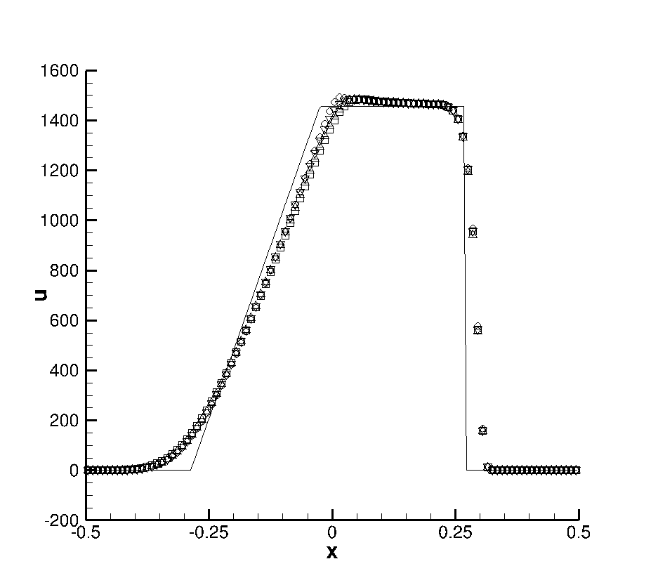
(b)

(c)

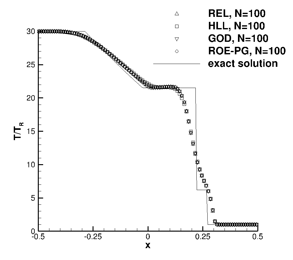
(d)

(a) $\rho$

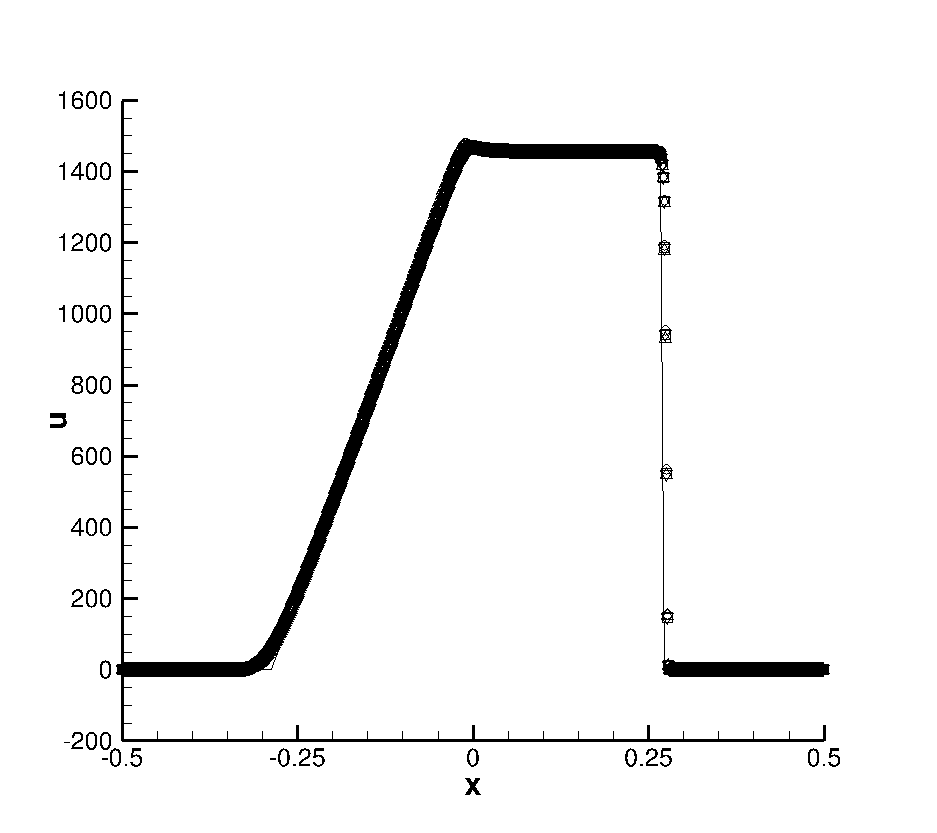
(b) $u$

(c) $\tfrac{\mathrm{p}}{\mathrm{p}_{R}}$

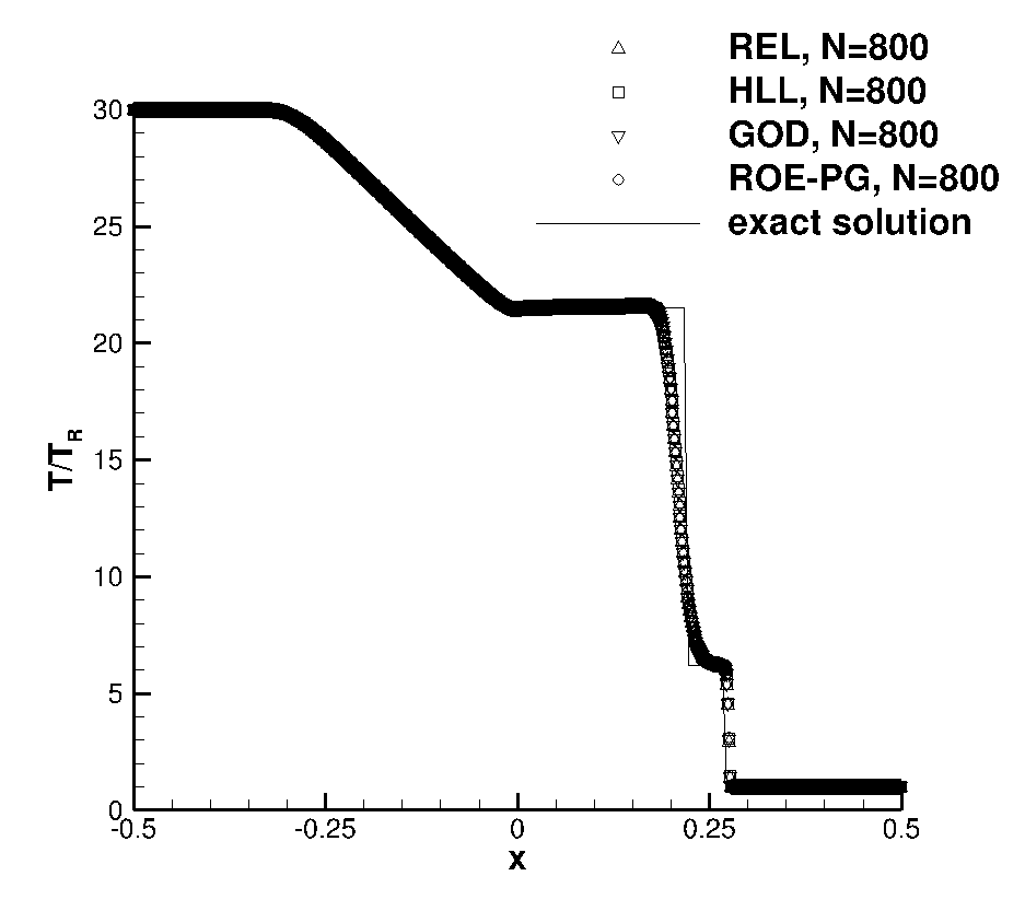
(d) $\tfrac{\mathrm{T}}{\mathrm{T}_{R}}$

Figure 3: Shock tube filled with air: results at time $t=1.5\times 10^{-4}$ obtained with the numerical fluxes 64 (REL), 60 (HLL), 58 (GOD), and the Roe solver for a monocomponent perfect gas (ROE-PG), on two grids with $N=100$ and $N=800$ elements.

6.2 Hypersonic flow over a sphere

We now consider the 2D hypersonic flow over a $\tfrac{1}{4}$ inch diameter sphere with the freestream conditions of Lobb’s experiments LOBB1964519 . The freestream Mach number is $M_{\infty}=\tfrac{u_{\infty}}{c_{\infty}}=15.3$ with $\rho_{\infty}=7.83\times 10^{-3}$kg/m³ and $\mathrm{T}_{\infty}=293$K. The upstream flow is made of nitrogen and oxigen with $Y_{N_{2}}=0.79$, $Y_{O_{2}}=0.21$ which are uniform in the flow domain since we do not consider chemical reactions or molecular relaxation. The freestream vibration temperatures are taken at $\mathrm{T}_{\infty}$ for both species. A symmetry condition is imposed at the bottom boundary.

(a)

(b)

Figure 4: Exemples of meshes for the 2D simulations: hypersonic flows over (a) a sphere with $N=100$ elements, (b) a double cone with $N=749$ elements.

Figure 5 displays the contours of Mach number and translation-rotation temperature on two different grids with the three different schemes. Neglecting chemical reactions overestimates the shock distance to the sphere and prevents comparison to Lobb’s experiments. As we do not consider chemical reactions or molecular relaxation, a partial validation of the current results can be obtained by comparison with simulations of an equivalent monocomponent perfect gas with adiabatic exponent $\gamma=1.4$. The simulations of the considered gas mixture using the numerical flux 60 and of the equivalent perfect gas using the HLL flux for polytropic gas dynamics (HLL-PG) are reported in fig. 6. As expected, while some differences can be identified for underresolved simulations, the results are almost perfectly overlapping for sufficiently fine resolutions.

We are however interested in comparing results obtained with the different schemes and analysing their convergence under grid refinement. To this end we compare the convergence of shock distance from the sphere in fig. 7. We use grids with $N=20\times 20$, $40\times 40$, $80\times 80$ and $160\times 160$ elements for the simulation (see fig. 4), while the reference distance $x_{ref}$ is evaluated with the Godunov numerical flux on a fine mesh with $N=320\times 320$. The results confirm convergence of the shock position and highlight close values obtained with the three different schemes.

(a)

(b)

(c)

(d)

(e)

(f)

(g)

(h)

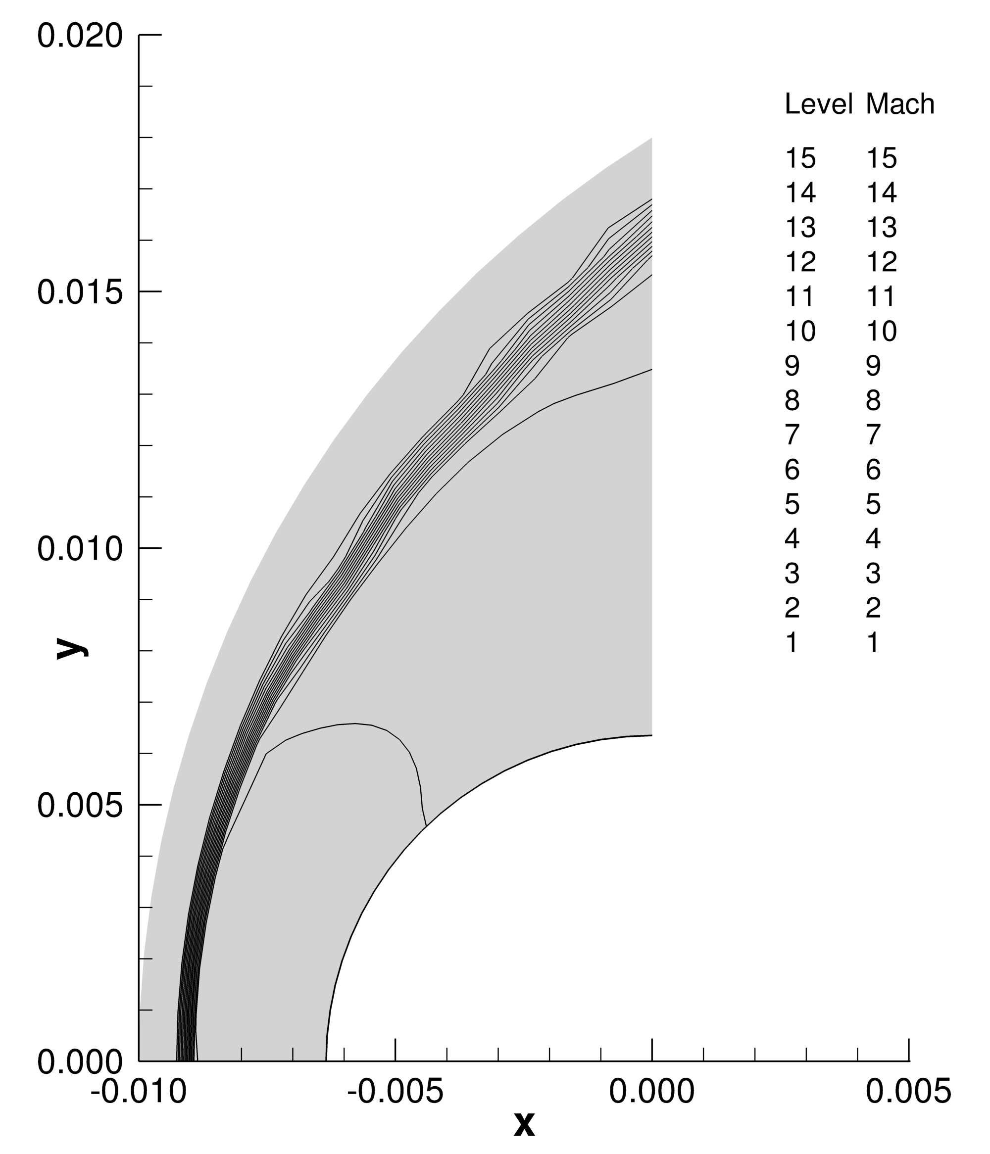
(a)

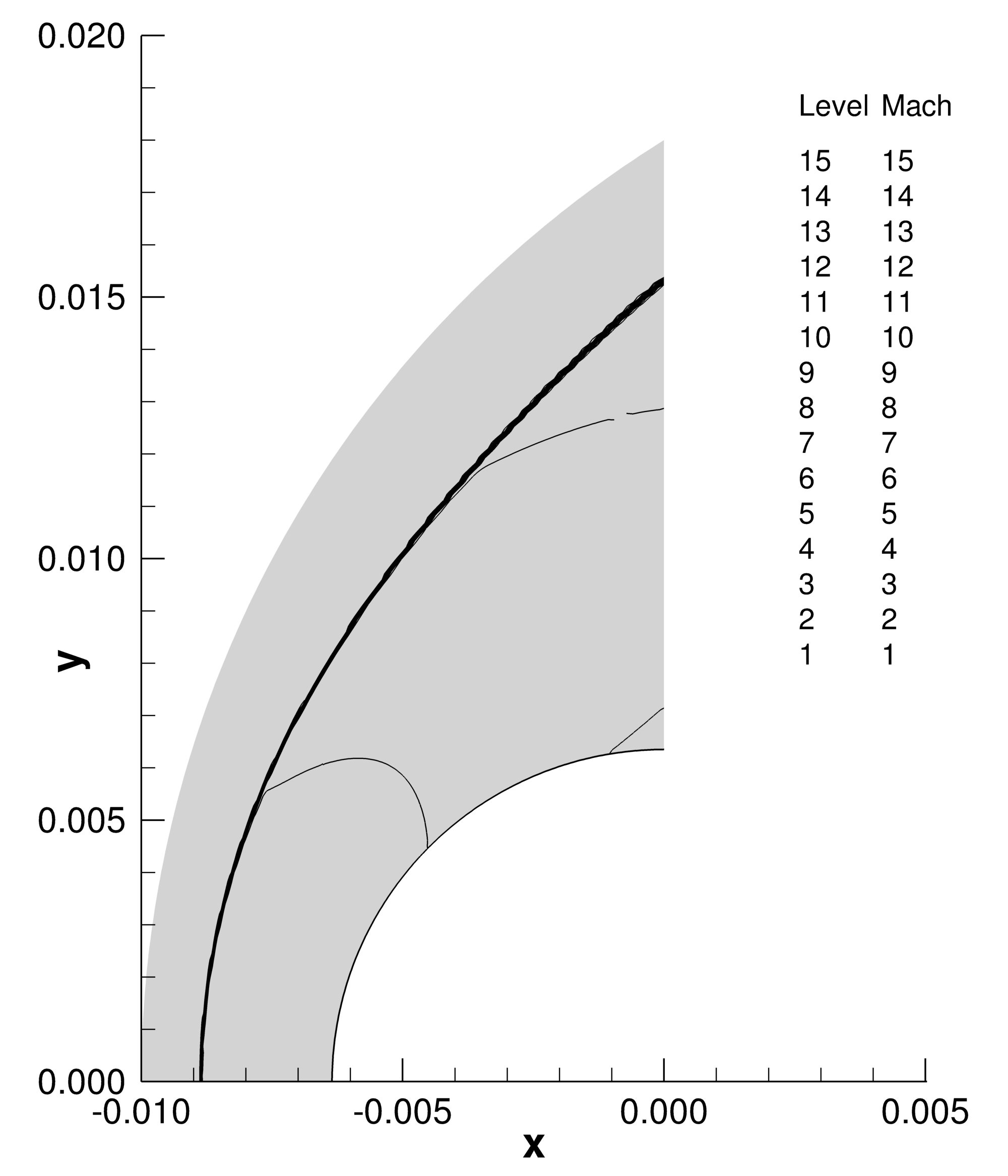
(b)

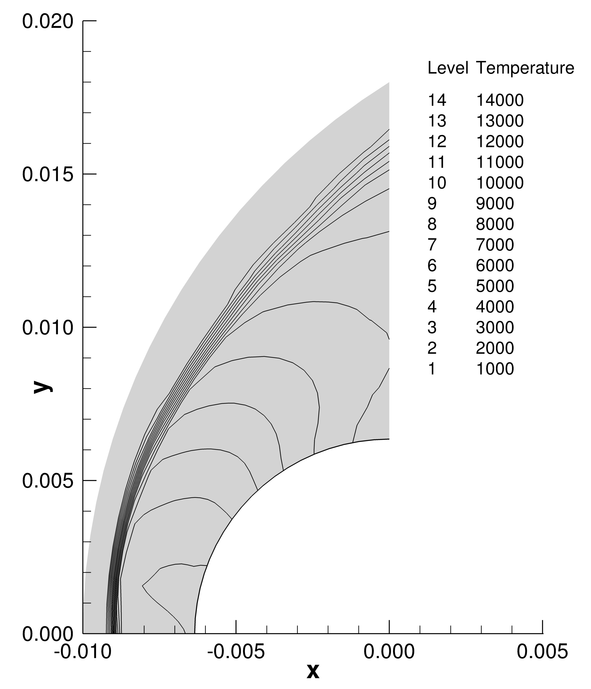
(c)

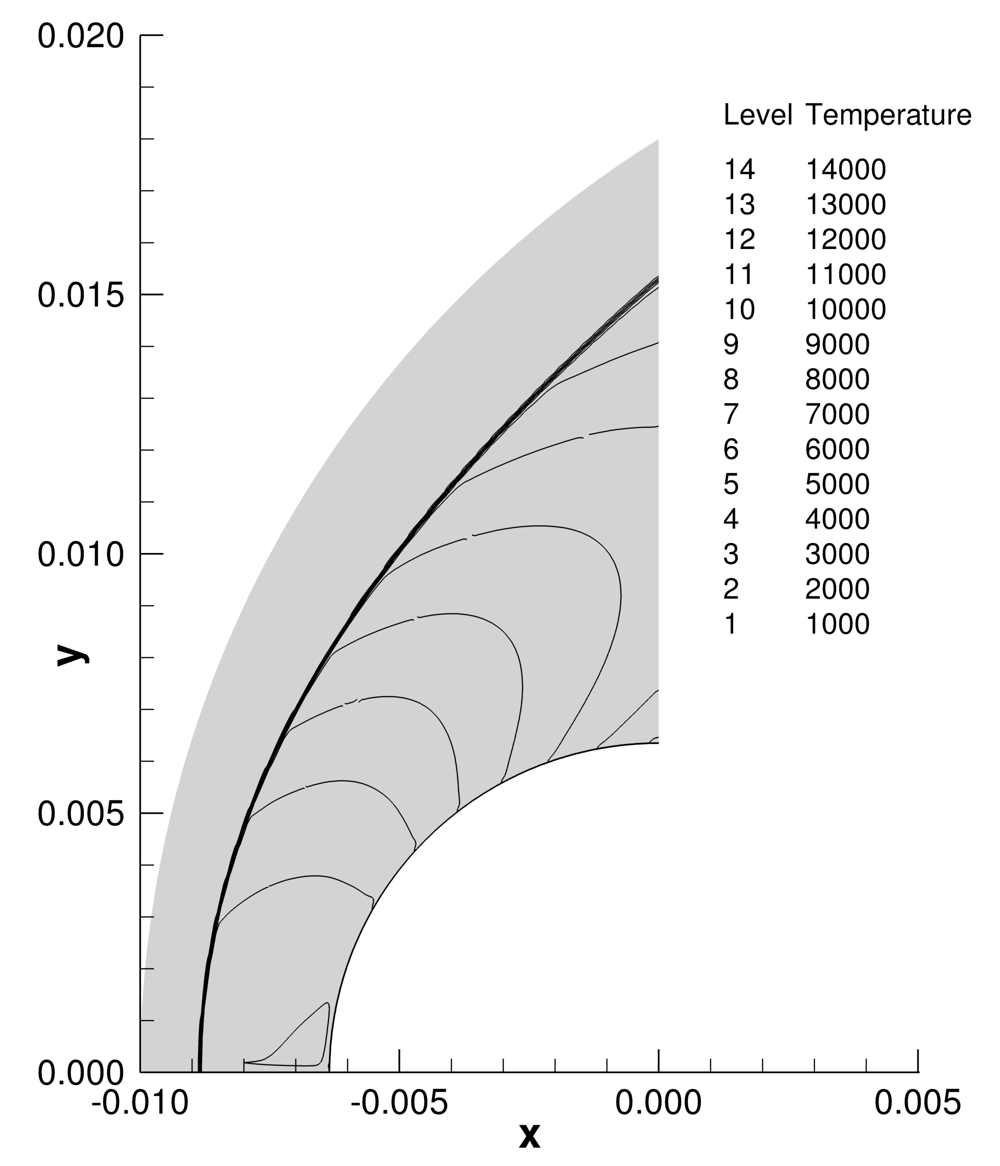
(d)

Figure 5: Hypersonic flow over Lobb’s sphere: Mach number $M$ and temperature $\mathrm{T}$ contours obtained with the numerical fluxes 64 (top row), 60 (middle row), 58 (bottom row), on two grids with $N=20\times 20$ and $160\times 160$ elements.

(a)

(b)

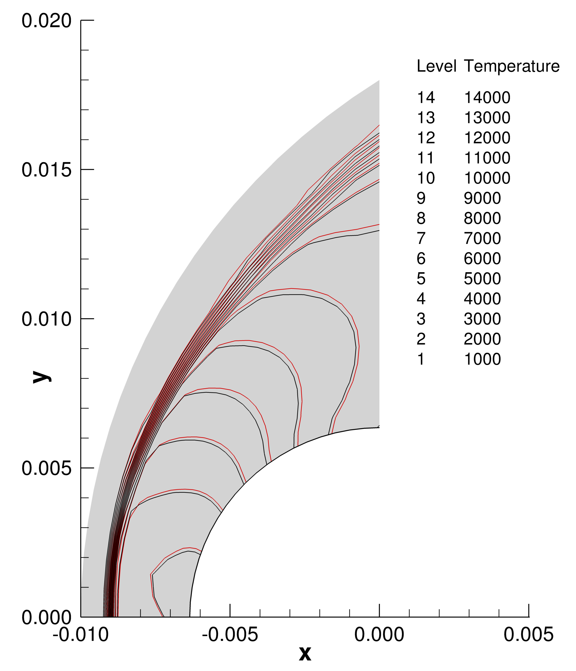
(c)

(d)

Figure 6: Hypersonic flow over Lobb’s sphere: Mach number $M$ and temperature $\mathrm{T}$ contours obtained with the HLL numerical flux 60 (red), and the HLL-PG flux considering an equivalent monocomponent perfect gas (black) on two grids with $N=20\times 20$ and $160\times 160$ elements.

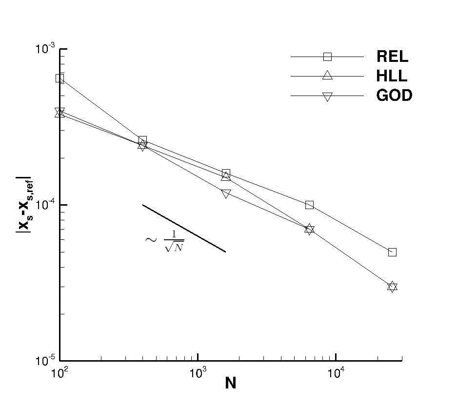
(a)

Figure 7: Hypersonic flow over Lobb’s sphere: convergence of the shock position in the symmetry plane $y=0$ under mesh refinement.

6.3 Hypersonic flow over a double cone

We finally consider the 2D hypersonic flow over a double cone with angles $25$ and $55$ deg. adapted from Druguet_et_al_05 ; KNIGHT20128 and made of molecular and atomic nitrogen with mass fractions $Y_{N_{2}}=0.99$, $Y_{N}=0.01$. The freestream Mach number is $M_{\infty}=11.3$ with $\rho_{\infty}=1.34\times 10^{-3}$kg/m³ and $\mathrm{T}_{\infty}=303$K. The freestream vibration temperature of the molecular nitrogen is taken at $\mathrm{T}_{N2_{\infty}}=3085$K. We use a series of five unstructured grids (see fig. 4). A symmetry condition is imposed at the bottom boundary.

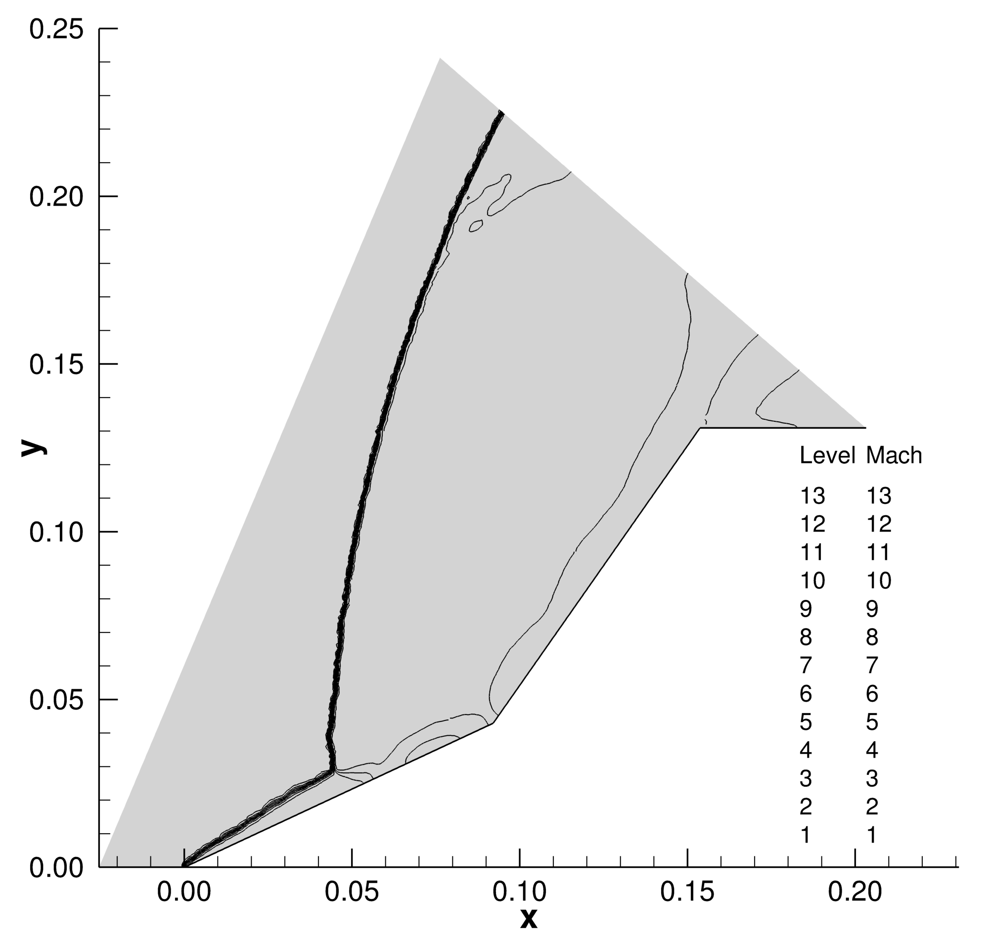
(a)

(b)

(c)

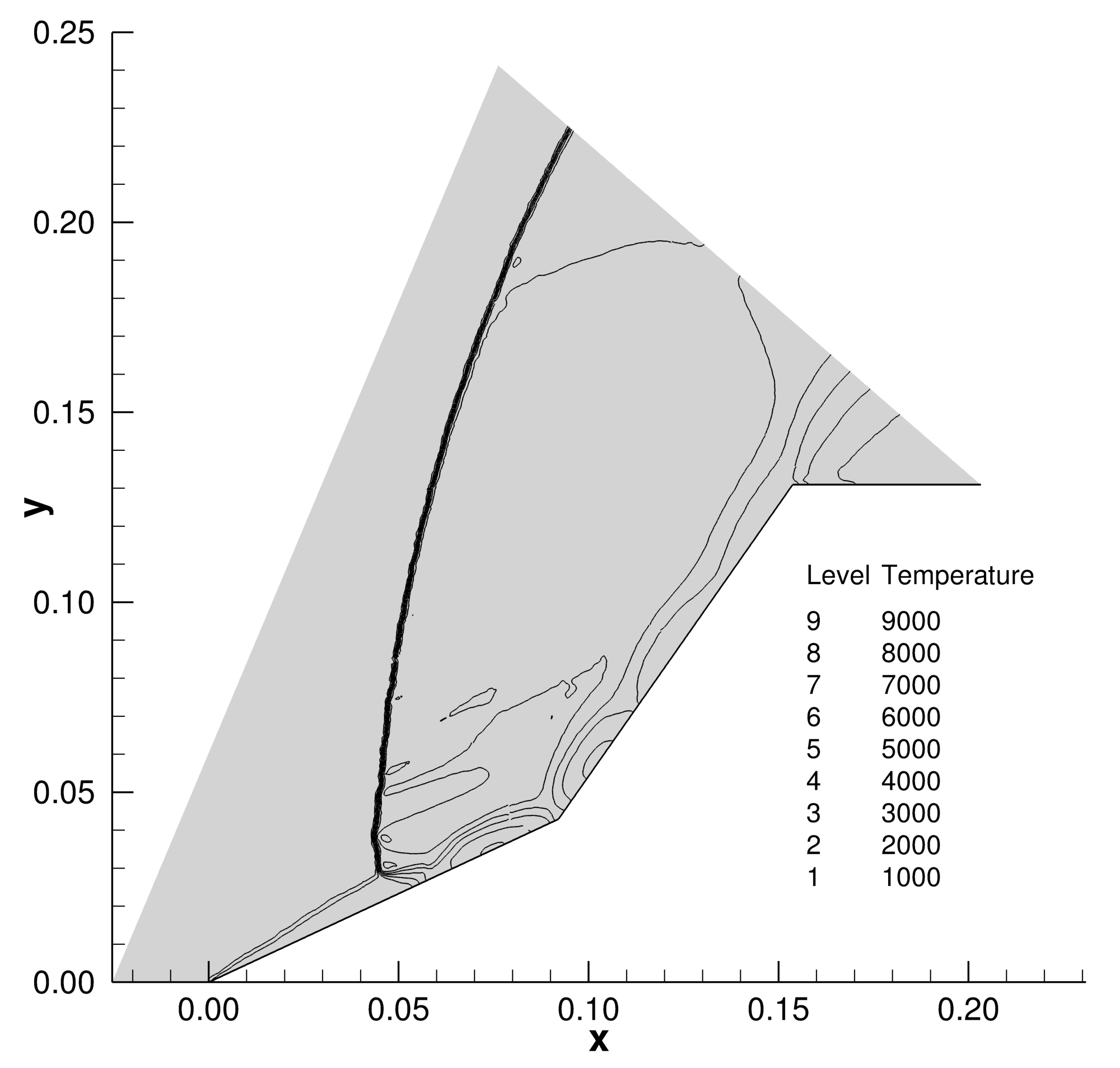
(a) REL

(b) HLL

(c) GOD

Figure 8: Hypersonic flow over a double cone: Mach number $M$ (top row) and temperature $\mathrm{T}$ (bottom row) contours obtained with the numerical fluxes 64 (REL), 60 (HLL), and 58 (GOD) on a fine grid with $N=52,237$ elements.

(a)

(b)

Figure 9: Hypersonic flow over a double cone: Mach number $M$ (left) and temperature $\mathrm{T}$ (right) contours obtained with the numerical flux 60 (red), and the HLL-PG flux considering an equivalent perfect gas (black) on a fine grid with $N=52,237$ elements.

Contours of Mach number and translation-rotation temperature obtained with the three different schemes on the second finest mesh are displayed in fig. 8. Compared to references Druguet_et_al_05 ; KNIGHT20128 , we observe a strong overestimation of the distance of the bow shock to the wall due to the absence of chemical reactions. However, the results with the three schemes are in good agreement. As done for the previous configuration, we compare in fig. 9 the obtained solution to that corresponding to the use of an equivalent perfect gas with adiabatic exponent $\gamma=1.4032$ (HLL-PG) on a fine grid. Once again a very good agreement is obtained. Finally in fig. 10, we display the pressure distribution at the wall obtained with the schemes on the five grids. The first pressure peak corresponds to the reflexion of the separated shock at the wall, while the second peak corresponds to rapid pressure variations due to the geometrical transition between the cones. We observe convergence of the solution as the mesh is refined and a close agreement between results from the three schemes on the finest grids.

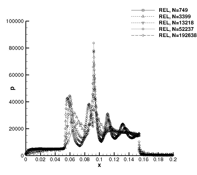
(a) REL

(b) HLL

(c) GOD

Figure 10: Hypersonic flow over a double cone: pressure distribution at the wall obtained with the numerical fluxes 64 (REL), 60 (HLL), and 58 (GOD) on a series of five grids with $N$ elements.

7 Concluding remarks

We introduce a general framework to design finite volume schemes for the compressible multicomponent Euler equations in thermal nonequilibrium. The framework allows to define a numerical scheme for its discretization from a scheme for the discretization of the monocomponent polytropic gas dynamics through a simple linear formula. Moreover, the numerical scheme inherits the properties of the scheme for the polytropic gas dynamics under a subcharacteristic condition on the adiabatic exponent of the polytropic gas.

This framework relies on the extension of the relaxation of energy for the gas dynamics equations coquel_perthame_98 to the model under consideration in this work. Three different numerical fluxes are constructed with this framework the polytropic Godunov exact Riemann solver godunov_59 , HLL numerical flux hll_83 , and pressure-based relaxation solver bouchut_04 . They are assessed through numerical simulations of flows in one and two space dimensions with discontinuous solutions and complex wave interactions. The results highlight robustness, nonlinear stability, convergence of the present method, as well as similar performances of the three schemes.

Other numerical fluxes may be deduced from this framework. We also stress that the numerical fluxes designed in this framework can be used as building blocks in the general framework of conservative elementwise flux differencing schemes fisher_carpenter_13 and future work will consider the use of discontinuous Galerkin schemes for the discretization of the compressible multicomponent Euler equations in thermal nonequilibrium.

Appendix A Convexity of the entropy for the energy relaxation system

The object of this appendix is the proof of lemma 2. Without loss of generality we define $n_{s}$ in the mapping 42 as the one corresponding to one species that satisfies $r_{n_{s}}=\min_{\alpha}r_{\alpha}$. To prove that $\rho\zeta({\bf w})$ is convex it is sufficient to prove that $\zeta(\boldsymbol{\cal Y},\tau,e_{r},e_{s},{\bf e}_{v})$ is convex from lemma 1 and, from 44, we rewrite $\zeta$ as

$$\zeta(\boldsymbol{\cal Y},\tau,e_{r},e_{s},{\bf e}_{v}) =C_{v_{t}}(\boldsymbol{\cal Y})\ln\big{(}(\gamma-\gamma(\boldsymbol{\cal Y}))C_{v_{t}}(\boldsymbol{\cal Y})\big{)}+\sum_{\alpha=1}^{n_{s}}r_{\alpha}Y_{\alpha}\ln Y_{\alpha}+\tfrac{r(\boldsymbol{\cal Y})}{\gamma-1}\ln\tfrac{\gamma(\boldsymbol{\cal Y})-1}{\gamma-\gamma(\boldsymbol{\cal Y})}$$

$$-r(\boldsymbol{\cal Y})\ln\tau-\tfrac{r(\boldsymbol{\cal Y})}{\gamma-1}\ln e_{r}-\tfrac{(\gamma-\gamma(\boldsymbol{\cal Y}))C_{v_{t}}(\boldsymbol{\cal Y})}{\gamma-1}\ln e_{s}+l(\boldsymbol{\cal Y})-\mathrm{s}_{v}({\bf Y},{\bf e}_{v}),$$

with $l(\boldsymbol{\cal Y})=-\sum_{\alpha}Y_{\alpha}C_{v_{\alpha}}^{t}\ln C_{v_{\alpha}}^{t}-C_{v_{t}}(\boldsymbol{\cal Y})\ln(\gamma-1)$, with $Y_{n_{s}}=1-\sum_{\alpha<n_{s}}Y_{\alpha}$, linear in $\boldsymbol{\cal Y}$.

Introducing the short notations $\partial_{k}r\equiv\partial_{Y_{k}}r(\boldsymbol{\cal Y})$, $\partial_{k}C_{v_{t}}\equiv\partial_{Y_{k}}C_{v_{t}}(\boldsymbol{\cal Y})$, and $\partial_{k}\gamma\equiv\partial_{Y_{k}}\gamma(\boldsymbol{\cal Y})$, the Hessian $\boldsymbol{\cal H}_{\zeta}(\boldsymbol{\cal Y},\tau,e_{r},e_{s},{\bf e}_{v})$ of $\zeta$ reads

$$\begin{pmatrix}\big{(}\partial_{kl}^{2}\zeta-\delta_{k,l}\psi_{k}\tfrac{e_{k}^{v^{2}}\mathrm{s}_{k}^{v^{\prime\prime}}\!\!(e_{k}^{v})}{Y_{k}}\big{)}_{kl}&\big{(}\tfrac{-\partial_{k}r}{\tau}\big{)}_{k}&\big{(}\tfrac{-\partial_{k}r}{(\gamma-1)e_{r}}\big{)}_{k}&\big{(}\tfrac{\partial_{k}r-(\gamma-1)\partial_{k}C_{v_{t}}}{(\gamma-1)e_{s}}\big{)}_{k}&\big{(}\tfrac{e_{k}^{v}\mathrm{s}_{k}^{v^{\prime\prime}}\!\!(e_{k}^{v})}{Y_{k}}\big{)}_{1\leq k\leq n_{d}}\\ \big{(}\tfrac{-\partial_{l}r}{\tau}\big{)}_{l}&\tfrac{r(\boldsymbol{\cal Y})}{\tau^{2}}&0&0&0\\ \big{(}\tfrac{-\partial_{l}r}{(\gamma-1)e_{r}}\big{)}_{l}&0&\tfrac{r(\boldsymbol{\cal Y})}{(\gamma-1)e_{r}^{2}}&0&0\\ \big{(}\tfrac{\partial_{l}r-(\gamma-1)\partial_{l}C_{v_{t}}}{(\gamma-1)e_{s}}\big{)}_{l}&0&0&\tfrac{\gamma-\gamma(\boldsymbol{\cal Y})}{\gamma-1}\tfrac{C_{v_{t}}(\boldsymbol{\cal Y})}{e_{s}^{2}}&0\\ \big{(}\tfrac{e_{l}^{v}\mathrm{s}_{l}^{v^{\prime\prime}}(e_{l}^{v})}{Y_{l}}\big{)}_{1\leq l\leq n_{d}}&0&0&0&\big{(}-\delta_{k,l}\tfrac{\mathrm{s}_{k}^{v^{\prime\prime}}\!\!(e_{k}^{v})}{Y_{k}}\big{)}_{k,l}\end{pmatrix}$$ (65)

with $\delta_{k,l}$ the Kronecker symbol and $\psi_{k}=1$ if $1\leq k\leq n_{d}$ and $\psi_{k}=0$ if $n_{d}<k<n_{s}$. Unless stated otherwise, the subscripts are in the range $1\leq k,l<n_{s}$, $k$ corresponding to a row index and $l$ corresponding to a column index. Likewise

$$\partial_{k}r\overset{\lx@cref{creftype~refnum}{eq:equiv-gamma}}{=}C_{v_{t}}(\boldsymbol{\cal Y})\partial_{k}\gamma+(\gamma(\boldsymbol{\cal Y})-1)\partial_{k}C_{v_{t}},$$ (66)

and

$$\partial_{kl}^{2}\zeta=\frac{r_{n_{s}}}{Y_{n_{s}}}+\frac{r_{k}}{Y_{k}}\delta_{k,l}+\frac{\partial_{k}C_{v_{t}}\partial_{l}C_{v_{t}}}{C_{v_{t}}(\boldsymbol{\cal Y})}+\frac{C_{v_{t}}(\boldsymbol{\cal Y})\partial_{k}\gamma\partial_{l}\gamma}{\big{(}\gamma-\gamma(\boldsymbol{\cal Y})\big{)}\big{(}\gamma(\boldsymbol{\cal Y})-1\big{)}},\quad 1\leq k,l<n_{s}.$$ (67)

We now prove that $\boldsymbol{\cal H}_{\zeta}$ is symmetric positive definite. Let ${\bf x}=(x_{1\leq i<n_{s}},x_{\tau},x_{r},x_{s},x_{1\leq i\leq n_{d}}^{v})^{\top}$ in $\mathbb{R}^{n_{s}+n_{d}+3}$ non zero and use the notation $\sum\equiv\sum_{k=1}^{n_{s}-1}$, we get

$$\sum_{k,l=1}^{n_{s}-1}x_{k}\partial_{kl}^{2}\zeta x_{l} \overset{\lx@cref{creftype~refnum}{eq:d2ZetadYY}}{=}\frac{r_{n_{s}}(\sum x_{k})^{2}}{Y_{n_{s}}}+\sum\frac{r_{k}x_{k}^{2}}{Y_{k}}+\frac{(\sum x_{k}\partial_{k}C_{v_{t}})^{2}}{C_{v_{t}}(\boldsymbol{\cal Y})}+\frac{C_{v_{t}}(\boldsymbol{\cal Y})(\sum x_{k}\partial_{k}\gamma)^{2}}{\big{(}\gamma-\gamma(\boldsymbol{\cal Y})\big{)}\big{(}\gamma(\boldsymbol{\cal Y})-1\big{)}}$$

$$\overset{\lx@cref{creftype~refnum}{eq:dr_dCv_dgam}}{=}\frac{r_{n_{s}}(\sum x_{k})^{2}}{Y_{n_{s}}}+\sum\frac{r_{k}x_{k}^{2}}{Y_{k}}+\frac{(\sum x_{k}\partial_{k}C_{v_{t}})^{2}}{C_{v_{t}}(\boldsymbol{\cal Y})}$$

$$+\frac{\Big{(}\sum x_{k}\big{(}\partial_{k}r-(\gamma(\boldsymbol{\cal Y})-1)\partial_{k}C_{v_{t}}\big{)}\Big{)}^{2}}{\big{(}\gamma-\gamma(\boldsymbol{\cal Y})\big{)}r(\boldsymbol{\cal Y})}$$

$$=\frac{r_{n_{s}}(\sum x_{k})^{2}}{Y_{n_{s}}}+\sum\frac{r_{k}x_{k}^{2}}{Y_{k}}+\frac{(\sum x_{k}\partial_{k}C_{v_{t}})^{2}}{C_{v_{t}}(\boldsymbol{\cal Y})}$$

$$+\frac{(\sum x_{k}\partial_{k}r)^{2}}{\big{(}\gamma-\gamma(\boldsymbol{\cal Y})\big{)}r(\boldsymbol{\cal Y})}+\frac{(\gamma(\boldsymbol{\cal Y})-1)(\sum x_{k}\partial_{k}C_{v_{t}})^{2}}{\big{(}\gamma-\gamma(\boldsymbol{\cal Y})\big{)}C_{v_{t}}(\boldsymbol{\cal Y})}-\frac{2(\sum x_{k}\partial_{k}r)(\sum x_{k}\partial_{k}C_{v_{t}})}{\big{(}\gamma-\gamma(\boldsymbol{\cal Y})\big{)}C_{v_{t}}(\boldsymbol{\cal Y})}$$

$$\overset{\lx@cref{creftype~refnum}{eq:dr_dCv_dgam}}{=}\frac{r_{n_{s}}(\sum x_{k})^{2}}{Y_{n_{s}}}+\sum\frac{r_{k}x_{k}^{2}}{Y_{k}}+\frac{(\sum x_{k}\partial_{k}r)^{2}}{(\gamma-1)r(\boldsymbol{\cal Y})}+\frac{(\sum x_{k}(\gamma-1)\partial_{k}C_{v_{t}}-x_{k}\partial_{k}r)^{2}}{\big{(}\gamma-\gamma(\boldsymbol{\cal Y})\big{)}(\gamma-1)C_{v_{t}}(\boldsymbol{\cal Y})},$$ (68)

so using 65 and 68 we obtain

$${\bf x}^{\top}\boldsymbol{\cal H}_{\zeta}{\bf x} =\frac{r_{n_{s}}(\sum x_{k})^{2}}{Y_{n_{s}}}+\sum\frac{r_{k}x_{k}^{2}}{Y_{k}}+\Big{(}1+\frac{1}{\gamma-1}-1\Big{)}\frac{(\sum x_{k}\partial_{k}r)^{2}}{r(\boldsymbol{\cal Y})}-\sum_{k=1}^{n_{d}}\tfrac{\mathrm{s}_{k}^{v^{\prime\prime}}\!(e_{k}^{v})}{Y_{k}}(x_{k}^{v}-e_{k}^{v}x_{k})^{2}$$

$$+\frac{(\sum x_{k}(\gamma-1)\partial_{k}C_{v_{t}}-x_{k}\partial_{k}r)^{2}}{\big{(}\gamma-\gamma(\boldsymbol{\cal Y})\big{)}(\gamma-1)C_{v_{t}}(\boldsymbol{\cal Y})}+r(\boldsymbol{\cal Y})\frac{x_{\tau}^{2}}{\tau^{2}}+\frac{r(\boldsymbol{\cal Y})}{\gamma-1}\frac{x_{r}^{2}}{e_{r}^{2}}$$

$$+\frac{\big{(}\gamma-\gamma(\boldsymbol{\cal Y})\big{)}C_{v_{t}}(\boldsymbol{\cal Y})}{\gamma-1}\frac{x_{s}^{2}}{e_{s}^{2}}-2\sum x_{k}\Big{(}\partial_{k}r\frac{x_{\tau}}{\tau}+\frac{\partial_{k}r}{\gamma-1}\frac{x_{r}}{e_{r}}+\frac{(\gamma-1)\partial_{k}C_{v_{t}}-\partial_{k}r}{\gamma-1}\frac{x_{s}}{e_{s}}\Big{)}$$

$$=Q({\bf x})+\frac{\big{(}\sum x_{k}\partial_{k}r-r(\boldsymbol{\cal Y})\tfrac{x_{\tau}}{\tau}\big{)}^{2}}{r(\boldsymbol{\cal Y})}+\frac{\big{(}\sum x_{k}\partial_{k}r-r(\boldsymbol{\cal Y})\tfrac{x_{r}}{e_{r}}\big{)}^{2}}{(\gamma-1)r(\boldsymbol{\cal Y})}$$

$$+\frac{\big{(}\sum x_{k}((\gamma-1)\partial_{k}C_{v_{t}}-\partial_{k}r)-(\gamma-\gamma(\boldsymbol{\cal Y}))C_{v_{t}}(\boldsymbol{\cal Y})\tfrac{x_{s}}{e_{s}}\big{)}^{2}}{(\gamma-\gamma(\boldsymbol{\cal Y}))(\gamma-1)C_{v_{t}}(\boldsymbol{\cal Y})}-\sum_{k=1}^{n_{d}}\tfrac{\mathrm{s}_{k}^{v^{\prime\prime}}\!(e_{k}^{v})}{Y_{k}}(x_{k}^{v}-e_{k}^{v}x_{k})^{2},$$

with $\mathrm{s}_{k}^{v^{\prime\prime}}\!(e_{k}^{v})=-\tfrac{r_{k}}{e_{k}^{v}(e_{k}^{v}+r_{k}\vartheta_{k}^{v})}<0$, so the four last terms are non-negative, and

$$Q({\bf x})=\frac{r_{n_{s}}(\sum x_{k})^{2}}{Y_{n_{s}}}+\sum\frac{r_{k}x_{k}^{2}}{Y_{k}}-\frac{(\sum x_{k}\partial_{k}r)^{2}}{r(\boldsymbol{\cal Y})}.$$

Using (43), we get $\partial_{k}r=r_{k}-r_{n_{s}}\geq 0$ since by assumption $r_{n_{s}}=\min_{\alpha}r_{\alpha}$, so we rewrite

$$\sum\frac{r_{k}x_{k}^{2}}{Y_{k}}=\sum\frac{r_{n_{s}}+\partial_{k}r}{Y_{k}}x_{k}^{2}=\sum\frac{r_{n_{s}}}{Y_{k}}x_{k}^{2}+\sum\frac{r_{n_{s}}+\sum_{l}Y_{l}\partial_{l}r}{r(\boldsymbol{\cal Y})}\frac{\partial_{k}r}{Y_{k}}x_{k}^{2},$$

and hence obtain

$$Q({\bf x}) =\frac{r_{n_{s}}(\sum x_{k})^{2}}{Y_{n_{s}}}+\sum\frac{r_{n_{s}}}{Y_{k}}\Big{(}1+\frac{\partial_{k}r}{r(\boldsymbol{\cal Y})}\Big{)}x_{k}^{2}+\sum_{k,l=1}^{n_{s}-1}\frac{\partial_{k}r\partial_{l}r}{r(\boldsymbol{\cal Y})}\Big{(}\frac{Y_{l}}{Y_{k}}x_{k}^{2}-x_{k}x_{l}\Big{)}$$

$$=\frac{r_{n_{s}}(\sum x_{k})^{2}}{Y_{n_{s}}}+\sum\frac{r_{n_{s}}}{Y_{k}}\Big{(}1+\frac{\partial_{k}r}{r(\boldsymbol{\cal Y})}\Big{)}x_{k}^{2}+\frac{1}{2}\sum_{k,l=1}^{n_{s}-1}\frac{\partial_{k}r\partial_{l}rY_{k}Y_{l}}{r(\boldsymbol{\cal Y})}\Big{(}\frac{x_{k}}{Y_{k}}-\frac{x_{l}}{Y_{l}}\Big{)}^{2},$$

which is positive, providing that the $x_{1\leq k<n_{s}}$ are not all zero since $\partial_{k}r\geq 0$, so ${\bf x}^{\top}\boldsymbol{\cal H}_{\zeta}{\bf x}>0$ and we conclude that $\zeta(\boldsymbol{\cal Y},\tau,e_{r},e_{s},{\bf e}_{v})$ is strictly convex. ∎

References

• (1) Abgrall, R.: How to prevent pressure oscillations in multicomponent flow calculations: a quasi conservative approach. J. Comput. Phys. 125(1), 150–160 (1996)
• (2) Anderson Jr., J.D.: Hypersonic and High Temperature Gas Dynamics. McGraw-Hill Book Company, New-York (1989)
• (3) Bouchut, F.: Nonlinear Stability of Finite Volume Methods for Hyperbolic Conservation Laws and Well-Balanced Schemes for Sources. Frontiers in Mathematics. Birkhäuser Basel (2004)
• (4) Candler, G.V., MacCormack, R.W.: Computation of weakly ionized hypersonic flows in thermochemical nonequilibrium. J. Thermophys. Heat. Trans. 5(3), 266–273 (1991). DOI 10.2514/3.260
• (5) Chen, G.Q., Levermore, C.D., Liu, T.P.: Hyperbolic conservation laws with stiff relaxation terms and entropy. Comm. Pure Appl. Math. 47(6), 787–830 (1994)
• (6) Ciarlet, P.: The Finite Element Method for Elliptic Problems. Classics in Applied Mathematics. Society for Industrial and Applied Mathematics (2002). URL https://books.google.fr/books?id=isEEyUXW9qkC
• (7) Colella, P., Glaz, H.M.: Efficient solution algorithms for the Riemann problem for real gases. J. Comput. Phys. 59(2), 264–289 (1985). DOI https://doi.org/10.1016/0021-9991(85)90146-9
• (8) Coquel, F., Godlewski, E., Perthame, B., In, A., Rascle, P.: Some New Godunov and Relaxation Methods for Two-Phase Flow Problems, pp. 179–188. Springer US, Boston, MA (2001)
• (9) Coquel, F., Godlewski, E., Seguin, N.: Relaxation of fluid systems. Math. Models Methods Appl. Science 22(08), 1250,014 (2012). DOI 10.1142/S0218202512500145
• (10) Coquel, F., Marmignon, C.: A Roe-type linearization for the Euler equations for weakly ionized multi-component and multi-temperature gas (19955). DOI 10.2514/6.1995-1675
• (11) Coquel, F., Perthame, B.: Relaxation of energy and approximate Riemann solvers for general pressure laws in fluid dynamics. SIAM J. Numer. Anal. 35(6), 2223–2249 (1998)
• (12) Dafermos, C.M.: Hyperbolic Conservation Laws in Continuum Physics. Grundlehren der mathematischen Wissenschaften. Springer Berlin Heidelberg, Berlin, Heidelberg (2016)
• (13) Dellacherie, Stéphane: Relaxation schemes for the multicomponent Euler system. ESAIM: M2AN 37(6), 909–936 (2003). DOI 10.1051/m2an:2003061. URL https://doi.org/10.1051/m2an:2003061
• (14) Drikakis, D.: Advances in turbulent flow computations using high-resolution methods. Progress in Aerospace Sciences 39(6), 405–424 (2003). DOI https://doi.org/10.1016/S0376-0421(03)00075-7
• (15) Druguet, M.C., Candler, G.V., Nompelis, I.: Effects of numerics on Navier-Stokes computations of hypersonic double-cone flows. AIAA Journal 43(3), 616–623 (2005). DOI 10.2514/1.6190
• (16) Einfeldt, B., Munz, C., Roe, P., Sjögreen, B.: On Godunov-type methods near low densities. J. Comput. Phys. 92(2), 273 – 295 (1991)
• (17) Fisher, T.C., Carpenter, M.H.: High-order entropy stable finite difference schemes for nonlinear conservation laws: Finite domains. J. Comput. Phys. 252, 518–557 (2013)
• (18) Flament, C., Prud’homme, R.: Entropy and entropy production in thermal and chemical non-equilibrium flows. J. Non-Equilib. Thermodyn. 18(4), 295–310 (1993). DOI https://doi.org/10.1515/jnet.1993.18.4.295. URL https://www.degruyter.com/view/journals/jnet/18/4/article-p295.xml
• (19) Gaitonde, D.: An Assessment of CFD for Prediction of 2-D and 3-D High-Speed Flows (2012). DOI 10.2514/6.2010-1284
• (20) Giovangigli, V.: Multicomponent Flow Modeling. Modeling and Simulation in Science, Engineering and Technology. Birkhäuser Basel (1999)
• (21) Glaister, P.: An approximate linearised Riemann solver for the three-dimensional Euler equations for real gases using operator splitting. J. Comput. Phys. 77(2), 361–383 (1988). DOI https://doi.org/10.1016/0021-9991(88)90174-X
• (22) Godlewski, E., Raviart, P.A.: Numerical approximation of hyperbolic systems of conservation laws. Applied Mathematical Sciences, vol. 118. Springer-Verlag, New-York (1996)
• (23) Godunov, S.: A difference scheme for numerical computation of discontinuous solutions of equations of fluid dynamics. Math. USSR Sbornik 47, 271–306 (1959)
• (24) Gouasmi, Ayoub, Duraisamy, Karthik, Murman, Scott M., Tadmor, Eitan: A minimum entropy principle in the compressible multicomponent Euler equations. ESAIM: M2AN 54(2), 373–389 (2020). DOI 10.1051/m2an/2019070. URL https://doi.org/10.1051/m2an/2019070
• (25) Guermond, J.L., Popov, B.: Fast estimation from above of the maximum wave speed in the Riemann problem for the Euler equations. J. Comput. Phys. 321, 908–926 (2016). DOI https://doi.org/10.1016/j.jcp.2016.05.054. URL http://www.sciencedirect.com/science/article/pii/S0021999116301991
• (26) Harten, A., Hyman, J.M.: Self adjusting grid methods for one-dimensional hyperbolic conservation laws. J. Comput. Phys. 50(2), 235–269 (1983). DOI https://doi.org/10.1016/0021-9991(83)90066-9
• (27) Harten, A., Lax, P.D., van Leer, B.: On upstream differencing and Godunov-type schemes for hyperbolic conservation laws. SIAM Rev. 25(1), 35–61 (1983)
• (28) Harten, A., Lax, P.D., Levermore, C.D., Morokoff, W.J.: Convex entropies and hyperbolicity for general Euler equations. SIAM J. Numer. Anal. 35(6), 2117–2127 (1998). DOI 10.1137/S0036142997316700
• (29) Henneton, M., Gainville, O., Coulouvrat, F.: Numerical simulation of sonic boom from hypersonic meteoroids. AIAA Journal 53(9), 2560–2570 (2015)
• (30) Honma, H., Glass, I.I.: Weak spherical shock-wave transitions of n-waves in air with vibrational excitation. Proceedings of the Royal Society of London. Series A, Mathematical and Physical Sciences 391(1800), 55–83 (1984)
• (31) Karni, S.: Hybrid multifluid algorithms. SIAM J. Sci. Comput. 17(5), 1019–1039 (1996). DOI 10.1137/S106482759528003X
• (32) Knight, D., Longo, J., Drikakis, D., Gaitonde, D., Lani, A., Nompelis, I., Reimann, B., Walpot, L.: Assessment of cfd capability for prediction of hypersonic shock interactions. Progress in Aerospace Sciences 48-49, 8–26 (2012). Assessment of Aerothermodynamic Flight Prediction Tools
• (33) Knisely, C.P., Zhong, X.: Sound radiation by supersonic unstable modes in hypersonic blunt cone boundary layers. ii. direct numerical simulation. Physics of Fluids 31(2), 024,104 (2019)
• (34) Liu, Y., Vinokur, M.: Nonequilibrium flow computations. i. an analysis of numerical formulations of conservation laws. J. Comput. Phys. 83(2), 373–397 (1989). DOI https://doi.org/10.1016/0021-9991(89)90125-3. URL http://www.sciencedirect.com/science/article/pii/0021999189901253
• (35) LOBB, R.K.: Chapter 26 - experimental measurement of shock detachment distance on spheres fired in air at hypervelocities. In: W.C. NELSON (ed.) The High Temperature Aspects of Hypersonic Flow, AGARDograph, vol. 68, pp. 519–527. Elsevier (1964). DOI https://doi.org/10.1016/B978-1-4831-9828-6.50031-X
• (36) PARK, C.: On convergence of computation of chemically reacting flows (1985). DOI 10.2514/6.1985-247
• (37) Park, C.: Nonequilibrium Hypersonic Aerothermodynamics. Springer-Verlag, New-York (1990)
• (38) Perthame, B., Shu, C.W.: On positivity preserving finite volume schemes for Euler equations. Numer. Math. 73(1), 119–130 (1996)
• (39) Prakash, A., Parsons, N., Wang, X., Zhong, X.: High-order shock-fitting methods for direct numerical simulation of hypersonic flow with chemical and thermal nonequilibrium. J. Comput. Phys. 230(23), 8474–8507 (2011)
• (40) Renac, F.: Entropy stable, robust and high-order DGSEM for the compressible multicomponent Euler equations. submitted (2020)
• (41) Renac, F., de la Llave Plata, M., Martin, E., Chapelier, J.B., Couaillier, V.: Aghora: A High-Order DG Solver for Turbulent Flow Simulations, pp. 315–335. Springer International Publishing, Cham (2015)
• (42) Roe, P.: Approximate Riemann solvers, parameter vectors, and difference schemes. J. Comput. Phys. 43(2), 357–372 (1981). DOI https://doi.org/10.1016/0021-9991(81)90128-5
• (43) Rouzaud, O., Chalons, C., Marmignon, C., Soubri’e, T.: Development of a Relaxation Scheme for Weakly Ionised Gases (2005). DOI https://doi.org/10.2514/6.2005-603
• (44) Rusanov, V.: Calculation of interaction of non-steady shock waves with obstacles. J. Comp. Math. Phys. USSR 1, 267–279 (1961)
• (45) Shuen, J.S., Liou, M.S., Leer, B.V.: Inviscid flux-splitting algorithms for real gases with non-equilibrium chemistry. J. Comput. Phys. 90(2), 371–395 (1990). DOI https://doi.org/10.1016/0021-9991(90)90172-W
• (46) Svärd, M., Özcan, H.: Entropy-stable schemes for the Euler equations with far-field and wall boundary conditions. J. Sci. Comput. 58, 61–89 (2014)
• (47) Tadmor, E.: A minimum entropy principle in the gas dynamics equations. Appl. Numer. Math. 6, 211–219 (1986)
• (48) Tadmor, E.: The numerical viscosity of entropy stable schemes for systems of conservation laws. i. Math. Comput. 49(179), 91–103 (1987)
• (49) Tadmor, E.: Entropy stability theory for difference approximations of nonlinear conservation laws and related time-dependent problems. Acta Numerica 12, 451–512 (2003)
• (50) Ton, V.T.: Improved shock-capturing methods for multicomponent and reacting flows. J. Comput. Phys. 128(1), 237–253 (1996). DOI https://doi.org/10.1006/jcph.1996.0206
• (51) Toro, E.F.: Riemann Solvers and Numerical Methods for Fluid Dynamics: A Practical Introduction. Third Edition. Springer-Verlag Berlin Heidelberg (2009)