Data-Driven Short-Term Voltage Stability Assessment Based on Spatial-Temporal Graph Convolutional Network

Abstract

Post-fault dynamics of short-term voltage stability (SVS) present spatial-temporal characteristics, but the existing data-driven methods for online SVS assessment fail to incorporate such characteristics into their models effectively. Confronted with this dilemma, this paper develops a novel spatial-temporal graph convolutional network (STGCN) to address this problem. The proposed STGCN utilizes graph convolution to integrate network topology information into the learning model to exploit spatial information. Then, it adopts one-dimensional convolution to exploit temporal information. In this way, it models the spatial-temporal characteristics of SVS with complete convolutional structures. After that, a node layer and a system layer are strategically designed in the STGCN for SVS assessment. The proposed STGCN incorporates the characteristics of SVS into the data-driven classification model. It can result in higher assessment accuracy, better robustness and adaptability than conventional methods. Besides, parameters in the system layer can provide valuable information about the influences of individual buses on SVS. Test results on the real-world Guangdong Power Grid in South China verify the effectiveness of the proposed network.

I Introduction

I-A Reseach background

WITH the rapid growth of power consumption, large-scale integration of renewable energy sources, and the increasing penetration of dynamic loads, short-term voltage instability has become the prominent problem in power systems [1]. When suffering from large disturbances, power systems may experience short-term voltage instability and trigger blackouts [2]. Blackouts can bring about huge economic losses and social impacts. Therefore, it is crucial to correctly assess voltage stability to take measures timely and prevent the occurrence of blackouts.

Recently, the rapid development of the wide-area measurement system (WAMS) has greatly promoted situational awareness of power systems. Phasor measurement units (PMUs) are widely deployed in the high-voltage stations of power systems. The PMU data is synchronized by the Global Position System (GPS) and can provide the real-time states of power systems [3]. The massive PMU data makes it feasible to conduct PMU data-driven short-term voltage stability (SVS) assessment, and it creates opportunities to provide SVS assessment results in a short time.

I-B Literature review

In general, there are mainly three categories of approaches for PMU data-driven stability assessment over past decades, namely the practical criteria, the stability mechanism-based methods, and machine learning-based methods. The widely accepted practical criterion is: when the duration of any bus voltage under a threshold exceeds the preset time [4], [5], the system is assessed as unstable. However, the threshold and the preset time all depend on the operating experiences of dispatchers, without any support from theory or enough data. Therefore, practical criteria lack reliability and adaptation. One of the typical stability mechanism-based methods is the maximum Lyapunov exponent (MLE) method [6]. This method can conduct SVS assessment with the sign of the MLE value. However, as the MLE value often oscillates around 0, it cannot provide a reliable result. In [7], the recovery time of equivalent induction motor rotation speed is estimated to assess SVS status. The accuracy of this method highly depends on the identification of induction motor parameters, while the identification of induction motor parameters is also a very difficult problem.

Machine learning-based methods have received much attention among researchers due to their superior performances. These methods learn the mapping between the input data and the final assessment results through the training dataset. Then, given the practical input data, the well-trained model can provide the assessment results based on the learned mapping. According to the use of input information, the existing machine learning-based assessment methods can be divided into three categories. The methods of the first category take single snapshots as the learning inputs, such as artificial neural network [8], ensemble model of neural networks with random weights (NNRW) [9], and ensemble model of extreme learning machine (ELM) [10]. However, with only single snapshots of time series, the temporal dynamics of SVS cannot be well characterized. To exploit the time-varying characteristics, the methods of the second category take post-fault time series as the learning input for stability assessment, such as shapelet-based methods [11], [12], long short-term memory (LSTM) model [13], and random vector functional link (RVFL) [14]. Nevertheless, apart from the time-varying characteristics, short-term voltage instability also presents spatial distribution characteristics [15]. Therefore, the methods of the third category take spatial-temporal information for stability assessment. The spatial-temporal characteristics of SVS have been neglected for years by most machine learning-based methods. To the best of the authors’ knowledge, there is only one attempt that incorporates spatial-temporal information, namely the spatial-temporal shapelet learning method [15]. This method incorporates spatial information into the learning model based on the geographical location information of the buses. However, the geographical locations may not exactly reflect the electrical distance between the buses, and the model based on geographical locations may not be accurate enough.

I-C Motivation and contribution

In fact, short-term voltage instability presents salient spatial-temporal characteristics. The affected region of short-term voltage instability exhibits spatial distribution characteristics and the low-voltage region reveals locality over topology. This phenomenon derives from the fact that reactive power cannot be transmitted over long distances and low voltage buses mainly affect electrically neighboring buses. Besides, the affected region of short-term voltage instability changes over time. However, these spatial-temporal characteristics haven’t been effectively incorporated into the learning model by the existing machine learning-based SVS assessment methods.

The key of getting an assessment model with good performances lies in the determination of input data and the design of the learning model. However, in the input data aspect, most of the existing methods fail to fully utilize the spatial-temporal information of the post-fault dynamics in SVS. Logically, the spatial-temporal characteristics in the post-fault dynamics haven’t been incorporated into the learning model. Once the topology information and temporal dynamics of post-fault measurements are combined together, the spatial-temporal characteristics of SVS could be fully exploited, resulting in a more credible SVS assessment model.

Therefore, in this paper, spatial-temporal graph convolutional network (STGCN) is developed to fully exploit the spatial-temporal characteristics of SVS and improve the performances of the SVS assessment model. Graph neural network is utilized to integrate topology information into the learning model and exploit the spatial information in SVS. Graph neural network has been widely used in social networks, transportation, chemistry, fault location in power distribution systems [16], etc. It has shown great advantages in tackling data residing on graphs [17], [18]. The foundation of graph neural network is graph convolutional network (GCN), which is powerful for incorporating spatial information. Therefore, it is adopted as the graph convolutional layer of the proposed STGCN. As for spatial-temporal information incorporation, there are mainly four ways by exploiting graph convolution: 1) adding a one-dimensional convolutional layer behind the graph convolutional layer [19]; 2) adding a long short-term (LSTM) layer or gated recurrent unit (GRU) behind the graph convolutional layer [20]; 3) modifying the original LSTM or GRU, which is to replace the fully connected layer in LSTM or GRU by graph convolution [21]; 4) representing temporal correlations as new edges of the graph and constructing a new graph with spatial-temporal correlations [22]. The second and third methods can achieve the incorporation of spatial-temporal information. However, the training time with LSTM or GRU-based method is longer than that with a one-dimensional convolutional layer. The fourth method constructs graph to treat temporal correlation with spatial correlation equally. It may not make sense due to the distinction between temporal correlations and spatial correlations.

Therefore, the one-dimensional convolutional layer is further adopted to enable spatial-temporal feature extraction from the hidden states of the graph convolutional layer. In this way, it incorporates spatial-temporal information with complete convolutional structures. Then, with consideration of SVS characteristics, a node layer is strategically designed to generate node representations for the buses. Based on the node representations, the system layer employs the simplified differentiable pooling [23] to provide the assessment result.

The main contributions of this paper are:

• A model framework with spatial-temporal information incorporation is developed in this paper. It successfully bridges the temporal data and topology information together to construct a model with higher performance.

• The spatial-temporal characteristics of SVS are first modeled with graph convolution and one-dimensional convolution. Combined with SVS characteristics, the proposed model can achieve higher accuracy, better robustness and adaptability.

• The influences of individual buses on SVS are provided and analyzed with the parameters in the designed system layer.

• Most existing works use the New England 39-bus system as the test system, which may not be large enough to fully test the performance of the learning model. In this paper, we use the real-world Guangdong Power Grid as the test system, which takes 101 high-voltage buses into account.

The remainder of this paper is organized as follows. A brief introduction of the proposed network for SVS assessment is given in Section II. In Section III, the design of STGCN is illustrated in detail. The real-world Guangdong Power Grid is utilized to test the performances of the proposed network in Section IV. Finally, conclusions are presented in Section V.

II Framework of STGCN for SVS assessment

II-A Online SVS assessment problem

SVS assessment is a tricky problem that has received long-term attention among researchers. Due to the high dimensionality, time-varying characteristics, and strong nonlinearity of SVS, the post-fault dynamics of SVS are very complex. Therefore, it is hard to achieve accurate online SVS assessment.

In fact, in large-scale complex power systems, the characteristics of short-term voltage instability can not only be reflected in post-fault responsive trajectories, but also spatial distribution. When severe faults happen, the affected regions of short-term voltage instability reveal obvious spatial distribution characteristics over topology, as shown in Fig. 1. This illustrative voltage distribution map is based on a snapshot of the post-fault voltage magnitude time series in the IEEE 39-bus test system. The legend on the right side of the map illustrates the correspondence between colors and voltage values. The region where the power system is located can be considered as a 2-D geographical space, and the map can be depicted with spatial voltage interpolation. As for the implementation of spatial voltage interpolation, the locations with real buses have their corresponding voltage values in the geographical space at the beginning. Spatial voltage interpolation means that the locations without real buses can be filled with virtual voltage values, and these virtual voltage values are estimated by geographical distance weighted interpolation. The detailed information about the spatial voltage interpolation can be found in [24].

As shown in Fig. 1, SVS exhibits salient spatial distribution characteristics over topology, and the low-voltage region reveals locality. If these characteristics are considered in the design of the learning model, it is feasible to achieve SVS assessment with higher performances.

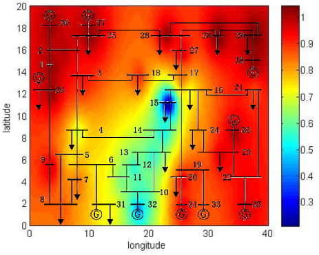
Figure 1: Illustrative voltage distribution map

II-B Graph neural network

Graph neural networks refer to a class of neural networks that can incorporate topology into the learning models and take advantage of graph dataset characteristics. They impose strong relational inductive biases on the network structure and are more appropriate for graph datasets than traditional convolution networks. Relational inductive biases refer to the constraints on the relationships and interactions among variables in a learning process. They can also be regarded as the assumptions about the data generation process or the space of solution [17]. Proper relational inductive biases in graph neural networks can improve model accuracy and generalization ability.

GCNs are the foundation of various graph neural networks. They can incorporate spatial information by graph convolution. GCNs fall into two categories of approaches, namely spectral theory-based approaches [25, 26, 27] and spatial-based approaches [28, 29, 30]. Spectral theory-based graph convolution is developed from graph signal processing domain. Its basic idea is to realize graph convolution by introducing filters from the perspective of graph signal processing. Spatial-based graph convolution is similar to the traditional convolution network. It is implemented as aggregating features from neighbors. It is more flexible, but no theoretical basis. As spectral theory-based graph convolution has a solid theoretical basis, it is adopted to incorporate spatial information into the learning model.

Spectral theory-based graph convolution networks study the properties of a graph by eigenvalues and eigenvectors of the normalized Laplacian matrix. The normalized Laplacian matrix is the mathematical representation of a graph, defined as

$$L=I_{n}-D^{-1/2}WD^{-1/2}$$ (1)

where $W$ is the adjacency matrix with weights, representing the connection relationships among nodes in the graph, $D$ is a diagonal matrix of the corresponding nodal degrees $D_{i,i}=\sum_{j}\left(W_{i,j}\right)$, and $I_{n}$ is an identity matrix. The normalized Laplacian matrix has real symmetric semi-definite properties, which can be factored as

$$L=U\Delta U^{T}$$ (2)

where $\Delta$ is a diagonal matrix composed of eigenvalues and $U$ is the matrix of eigenvectors ordered by eigenvalues. The graph Fourier transform to a signal x is defined as $F(x)=U^{T}x$. $U^{T}$ is regarded as the graph Fourier basis.

The graph convolution of the input signal $x$ with filter $g$ is defined as

$$x*Gg=U(U^{T}x\bigodot U^{T}g)$$ (3)

where $\bigodot$ denotes the Hadamard product. If the filter is denoted as $g_{\theta}=\operatorname{diag}\left(U^{T}g\right)$, the graph convolution can be simplified as

$$x*Gg=Ug_{\theta}U^{T}x$$ (4)

All graph convolution networks based on spectral theory follow this definition, but the filters $g_{\theta}$ are different.

II-C Novel framework for SVS assessment

To exploit the spatial distribution characteristics of SVS, graph convolution is utilized to integrate topology information into the learning model. Then, the spatial-temporal information incorporation block with the graph convolutional layer is designed to extract the spatial-temporal features of SVS. In fact, the stacking number of the spatial-temporal information incorporation blocks can represent the reception fields of the buses. In order to capture spatial-temporal features from different reception fields, several spatial-temporal information incorporation blocks are stacked, and the fusion information from each spatial-temporal information incorporation block is utilized for SVS assessment.

As a matter of fact, voltage stability is regarded as load stability for a long time. Although it may not be accurate enough, the state of load buses can affect voltage stability to a large extent. Therefore, the node layer block is designed to generate the node representations of the buses after the spatial-temporal information incorporation blocks. Then, based on the node representations, the system layer block is utilized to provide the final SVS assessment result.

The framework of the proposed STGCN to conduct the SVS assessment task is shown in Fig. 2. The input data will be processed by three parts, the spatial-temporal information incorporation blocks, the node layer block, and the system layer block. This framework incorporates the characteristics of SVS into the learning model and is more appropriate for online SVS assessment. The detailed information about these blocks will be illustrated in Section III.

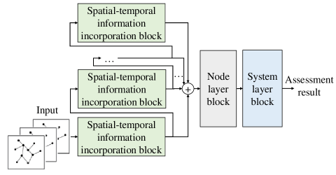
Figure 2: The framework of STGCN

The implementation of the proposed network for SVS assessment can be divided into two stages, the offline training stage and the online assessment stage. At the offline training stage, a large number of samples are generated with electromechanical transient analysis programs. Then, the database can be formed with post-fault time series and topology of these samples as the inputs and the corresponding stability status as the output. Time series for the inputs consist of voltage magnitude, active power injection, and reactive power injection time series. With the prepared database, STGCN can be trained with gradient descent algorithms, such as the Adam algorithm [31]. When the testing accuracy of STGCN reaches a preset threshold, the trained STGCN will be saved for online assessment. At the online assessment stage, post-fault PMU measurements and topology of the observed region can be obtained as the inputs. Then, the trained STGCN is utilized to conduct SVS assessment. If the assessment result shows that the system is stable, then the model continues to monitor. If the assessment result shows that the system is unstable, warning signals will be sent out to remind operators to take measures.

III Design of STGCN

III-A Definition of the input layer

SVS assessment is a typical multivariate time series classification task. In this paper, it is assumed that voltage magnitude time series $V_{t}$, active power injection time series $P_{t}$ and reactive power injection time series $Q_{t}$ are available and of great importance for SVS. Therefore, these multivariate time series are utilized as the inputs of the proposed network

$$V_{t} =\begin{bmatrix}v_{1}&v_{2}&...&v_{n}\end{bmatrix}$$ (5)

$$P_{t} =\begin{bmatrix}p_{1}&p_{2}&...&p_{n}\end{bmatrix}$$ (6)

$$Q_{t} =\begin{bmatrix}q_{1}&q_{2}&...&q_{n}\end{bmatrix}$$ (7)

where $t=1,2,...,N$, $N$ is the number of time points for stability assessment, $n$ is the number of observed buses.

As short-term voltage instability presents spatial distribution characteristics, the topology $W$ of the observed region is also extracted as the input. More specifically, the topology matrix $W$ is composed of a node admittance matrix. When the topology of the observed region changes, the topology matrix also changes, thereby adapting to the changes of topology.

$$W =\begin{bmatrix}w_{11}&w_{12}&...&w_{1n}\\ w_{21}&w_{22}&...&w_{2n}\\ ...&...&...&...\\ w_{n1}&w_{n2}&...&w_{nn}\\ \end{bmatrix}$$ (8)

The illustrative figure for the input data of STGCN is shown in Fig. 3.

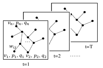
Figure 3: The input data for ST-GCN

III-B Spatial-temporal information incorporation blocks

Spatial-temporal information incorporation blocks are formed by stacking several spatial-temporal information incorporation blocks and utilizing the fusion information from each spatial-temporal information incorporation block.

Each spatial-temporal information incorporation block consists of four parts, a graph convolutional layer, a temporal convolutional layer, a normalization layer, and a dropout layer. The graph convolutional layer is adopted to incorporate spatial information and extract spatial features. The temporal convolutional layer is adopted to incorporate temporal information and extract temporal features. In order to prevent over-fitting, a normalization layer and a dropout layer are added to improve the performances of the proposed network. The detailed illustration of one spatial-temporal information incorporation block is shown in Fig. 4.

III-B1 The graph convolution layer

As spectral theory-based graph convolution has a solid theoretical basis, it is adopted to incorporate spatial information. The first spectral convolution neural network is proposed by Bruna [25]. The corresponding filter is defined as $g_{\theta}=\theta_{i,j}^{k}$. As the computation of the graph Fourier basis can cost lots of time, Defferrard proposes Chebyshev spectral convolution neural network (ChebNet) [26]. This method defines filters as Chebyshev polynomials of the eigenvalue diagonal matrix. When only using the first polynomial, it turns into the first-order approximation of ChebNet [27]. Due to the less computational complexity and locality of Chebyshev filter, ChebNet is adopted to extract the spatial features in SVS assessment.

ChebNet defines filters as Chebyshev polynomials of the eigenvalue diagonal matrix

$$g_{\theta}={\sum}_{i=0}^{K}{\theta}_{i}T_{i}(\tilde{\Delta})$$ (9)

where $\tilde{\Delta}=2\Delta/{\lambda}_{max}-I_{n},T_{i}(\tilde{\Delta})=2\tilde{\Delta}T_{i-1}(\tilde{\Delta})-T_{i-2}(\tilde{\Delta})$ with $T_{0}(\tilde{\Delta})=1$, $T_{1}(\tilde{\Delta})=\tilde{\Delta}$. ${\lambda}_{max}$ is the maximal eigenvalue, ${\theta}_{i}$ is the learnable parameter and $K$ is the Chebyshev order.

The input signal for graph convolution can be voltage magnitude time series, active power injection time series and reactive power injection time series. The graph convolution of voltage magnitude $V_{t}$ with filter $g_{\theta}$ in a time step can be represented as

$$V_{t}*Gg_{\theta} =U({\sum}_{i=1}^{K}{\theta}_{Vi}T_{i}(\tilde{\Delta}))U^{T}V_{t}$$ (10)

$$={\sum}_{i=0}^{K}{\theta}_{Vi}T_{i}(\tilde{L})V_{t}$$ (11)

The graph convolution of voltage magnitude $P_{t}$ with filter $g_{\theta}$ in a time step can be represented as

$$P_{t}*Gg_{\theta} =U({\sum}_{i=1}^{K}{\theta}_{Pi}T_{i}(\tilde{\Delta}))U^{T}P_{t}$$ (12)

$$={\sum}_{i=0}^{K}{\theta}_{Pi}T_{i}(\tilde{L})P_{t}$$ (13)

The graph convolution of voltage magnitude $Q_{t}$ with filter $g_{\theta}$ in a time step can be represented as

$$Q_{t}*Gg_{\theta} =U({\sum}_{i=1}^{K}{\theta}_{Qi}T_{i}(\tilde{\Delta}))U^{T}Q_{t}$$ (14)

$$={\sum}_{i=0}^{K}{\theta}_{Qi}T_{i}(\tilde{L})Q_{t}$$ (15)

where ${\theta}_{V}$, ${\theta}_{P}$, ${\theta}_{Q}$ are the learned paprameters in the graph convlutional layer, $T_{i}(\tilde{L})=2\tilde{L}T_{i-1}(\tilde{L})-T_{i-2}(\tilde{L})$ with $T_{0}(\tilde{L})=1$, $T_{1}(\tilde{L})=\tilde{L}$, $\tilde{L}=2L/\lambda_{\max}-I_{n}$, $L=I_{n}-D^{-1/2}WD^{-1/2}$ and $W$ indicates the topology of the observed region.

$T_{i}(\tilde{L})$ is Chebyshev filter matrix, which is the key element to realize graph convolution. In the graph convolutional layer, each bus updates its node information according to the information in its reception field. The locality of Chebyshev filter matrix ensures that the buses in the reception field of one bus are its neighboring buses. It is consistent with the spatial distribution characteristics of SVS.

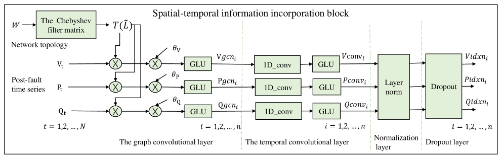
Figure 4: The spatial-temporal information incorporation block

After the graph convolution of the input time series, the activation function, such as the gated linear unit (GLU) [32], is utilized to model the nonlinear characteristics of SVS. $Vgcn_{i}$, $Pgcn_{i}$, $Qgcn_{i}$ are the data processed by the graph convolutional layer, $Vgcn_{i}=[vgcn_{1}\quad vgcn_{2}\quad...\quad vgcn_{N}]^{T}$, $Pgcn_{i}=[pgcn_{1}\quad pgcn_{2}\quad...\quad pgcn_{N}]^{T}$, $Qgcn_{i}=[qgcn_{1}\quad qgcn_{2}\quad...\quad qgcn_{N}]^{T}$.

III-B2 The temporal convolution layer

After the extraction of spatial features, the one-dimensional convolution is adopted to incorporate temporal information and extract temporal features. After that, the activation function, such as gated linear unit (GLU), is utilized to model the nonlinear characteristics of SVS

$$Vconv_{i}=GLU(1D\_conv(Vgcn_{i}))$$ (16)

$$Pconv_{i}=GLU(1D\_conv(Pgcn_{i}))$$ (17)

$$Qconv_{i}=GLU(1D\_conv(Qgcn_{i}))$$ (18)

where ${Vconv}_{i}$,${Pconv}_{i}$,${Qconv}_{i}$ are the data processed by the temporal convolution layer, $i=1,2,..,n$.

Then, the normalization layer and dropout layer are added to prevent over-fitting, and the data are transformed as $Vidxn_{i}$, $Pidxn_{i}$, $Qidxn_{i}$.

When stacking several spatial-temporal information incorporation blocks, to distinguish the data processed by different blocks, the data $Vidxn_{i}$, $Pidxn_{i}$, $Qidxn_{i}$ are further denoted as $Vidxn_{i,j}$, $Pidxn_{i,j}$, $Qidxn_{i,j}$, and $j$ is utilized for distinguishing different blocks.

III-B3 Spatial-temporal convolution incorporation blocks

To capture spatial-temporal features from different reception fields, $L_{c}$ spatial-temporal information incorporation blocks are stacked, and the fusion information from each spatial-temporal information incorporation block is utilized for SVS assessment.

$$Pidxz_{i}=\sum_{j=1}^{L_{c}}Pidxn_{i,j}$$ (19)

$$Qidxz_{i}=\sum_{j=1}^{L_{c}}Qidxn_{i,j}$$ (20)

$$Vidxz_{i}=\sum_{j=1}^{L_{c}}Vidxn_{i,j}$$ (21)

where $i=1,2,..,n$, ${Vidxz}_{i}$, ${Pidxz}_{i}$, ${Qidxz}_{i}$ are the data processed by the fusion of the spatial-temporal information incorporation blocks.

III-C Node layer block and system layer block

III-C1 Node layer block

After extracting the spatial-temporal features of different channels, namely voltage magnitude channel, active power injection channel, and reactive power injection channel, new representations of different channels on each bus can be obtained.

The node layer block is utilized to convert them into a single representation on each bus by applying a weighted summation on different channels. Then, the data are processed by a normalization layer and the absolute values are taken as their node representations

$$Snode_{i}=|Layernorm( {\psi}_{1}*Pidxz_{i}+{\psi}_{2}*Qidxz_{i}$$

$$+{\psi}_{3}*Vidxz_{i})|$$ (22)

where ${Snode}_{i}$ is the node representation of bus $i$, ${\psi}_{1}$, ${\psi}_{2}$, ${\psi}_{3}$ are the weights in the node layer representation block.

III-C2 System layer block

Based on the node representations, the SVS status of the target region can be obtained in three ways, namely max/mean pooling, multi-layer perceptron plus softmax function, and differentiable pooling layer [23]. The differentiable pooling layer can generate hierarchical representations of a graph, showing better performances than other graph pooling methods. Based on the node representation, the differentiable pooling layer is simplified as the system layer to provide the SVS assessment result. It is defined as follows

$$Ssys=softmax(SNODE*softmax(Sb)^{T})$$ (23)

where $SNODE=[Snode_{1}\quad Snode_{2}\quad...\quad Snode_{n}]$, $Sb$ is the dense learned assignment matrix, $Sb\in\mathbb{R}^{2\times n}$, $Ssys$ is the SVS assessment result, $Ssys\in\mathbb{R}^{1\times 2}$. Softmax function is used as the final function of the network. It can provide probability values for different categories [33], [34]. The predicted category of a sample is the corresponding category of the column with the highest probability value. For binary classification in SVS assessment, the probability value in the first column of $Ssys$ is set to represent the probability of stable status, and the probability value in the second column of $Ssys$ is set to represent the probability of unstable status. Therefore, if the element of $Ssys$ in the first column is greater than the element of $Ssys$ in the second column, the system is stable, otherwise, it is unstable. Cross entropy loss function is adopted as the loss function of the proposed network.

The elements of $softmax(Sb)^{T}$ in the first column minus the elements of $softmax(Sb)^{T}$ in the second column are regarded as the learned parameters $S$ in the system layer. With the node representations $SNODE$ and learned parameters $S$ in the system layer, the SVS status can also be obtained by multiplying these two matrices. When the final result is positive, the target region is stable, otherwise, it is unstable. As the absolute values are taken as the node representations, the sign of parameters $S$ in the system layer can directly affect the assessment result. Therefore, the positive/negative weight values $S$ can indicate the beneficial/detrimental influences of corresponding buses on SVS.

IV Case study

IV-A System description and simulation setting

The proposed network is tested on the real-world Guangdong Power Grid. Guangdong Power Grid is a typical receiving-end system of China Southern Power Grid. It is prone to suffer from the voltage instability problem. Therefore, Guangdong Power Grid is utilized for SVS assessment. The backbone structure of Guangdong Power Grid is shown in Fig. 5. There are 101 high-voltage buses in Guangdong Power Grid. All high-voltage buses in Guangdong Power Grid are assumed to be installed with PMUs. These PMU measurements are utilized for online monitoring. All loads in the system are represented by the composite load model consisting of induction motor and static loads.

Samples are generated by PSD-BPA software, which is the power system simulation software widely used by Chinese power companies. 5400 cases are generated with PSD-BPA software by setting different fault locations, different fault clearing time, and different induction motor ratios. More specifically, the fault clearing time is set to 0.1, 0.2, 0.3, 0.4, 0.5 seconds. The induction motor ratio is set to 0.3, 0.5, 0.7, 0.9. Three-phase short-circuit faults are imposed on 270 different fault locations which are randomly selected from the high-voltage transmission lines in Guangdong Power Grid. Besides, to consider topology changes, 600 cases are generated with PSD-BPA software by setting different topology changes, different fault clearing time, and different induction motor ratios. More specifically, the fault clearing time is set to 0.5, 1.0, 1.5 seconds to simulate severe situations, and the induction motor ratio is set to 0.7 and 0.9. Each of these topology changes in the dataset contains a one-part change of the original topology. In addition, the transient simulation in each case lasts 10 seconds after fault clearance. These 6000 cases are randomly mixed and utilized to test the performances of the proposed network. Besides, more cases are generated in the later subsections to fully test the performances of the proposed model under different kinds of environments.

For each case, the 10-second post-fault trajectory data is used to provide an output label according to the stability status. The topology, namely the node admittance matrix, is extracted to form the input topology matrix. The data of one second after fault clearance, including voltage magnitude, active power injection, and reactive power injection time series, are used as the input time series. In fact, the length of the observation window for SVS assessment can affect classification accuracy. The longer the observation window, the higher the assessment accuracy. However, SVS assessment in practice also requires earliness. The observation window used in this article is a typical setting in the related researches [15]. Besides, the proposed method is also available for temporal-adaptive implementation referring to the scheme proposed in [10], [13].

With the prepared dataset, STGCN is adopted for training. STGCN is conducted in Python with TensorFlow. As for the setting of hyperparameters, the batch size is set to 100, the training epoch is set to 30, the step in one epoch is set to 48, and the learning rate is set to 0.001. Chebyshev order K is set to 2. Five spatial-temporal information incorporation blocks are stacked and the fusion information is utilized for SVS assessment.

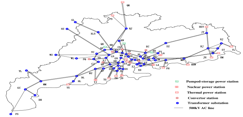
Figure 5: Backbone structure of Guangdong Power grid

IV-B STGCN training performances

This subsection aims to illustrate the effectiveness of the proposed network and each part in STGCN. First, the effectiveness of the overall network is investigated with training loss value, training accuracy, and five-fold cross-validation results. Then, according to the data processing order in STGCN, the effectiveness of each part is illustrated. First, the locality of Chebyshev filter matrix is illustrated. Then, the effectiveness of spatial-temporal feature extraction and node layer representation is illustrated by the visualization of the processed data. Finally, this paper verifies the effectiveness of the system layer for identification of the influences of individual buses on SVS.

IV-B1 Effectiveness of the overall network

The distributions of loss value and accuracy in the training process are shown in Fig. 6. As shown in the two figures, the proposed network shows fast convergence at the beginning of the training process, and the training accuracy reaches over 95% after 10 training epochs. With the increase of training time, the loss value gradually decreases, and the training accuracy increases. The fluctuation range of loss value and training accuracy also gradually decreases. Finally, the loss value eventually stables near zero, and the training accuracy stables near 99%. Such a training process illustrates that the training is effective and the model is developing in the right direction. With the proposed network, five-fold cross-validation is conducted. The average training accuracy of the model reaches 99.4%, and the average testing accuracy reaches 98.8%. The good performance illustrates the effectiveness of the proposed network.

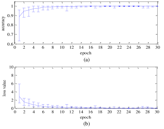
Figure 6: The distributions of loss value and accuracy in training process

IV-B2 Locality of Chebyshev filter Matrix

The Chebyshev filter matrix, namely $T_{i}(\tilde{L})$, is the key element to realize graph convolution. The locality of the Chebyshev filter matrix ensures that the buses only exchange information with their neighboring buses, which is consistent with the spatial characteristics of SVS.

To illustrate the locality of Chebyshev filter matrix, Chebyshev filter matrices of different orders and the corresponding reception fields of MM station in Guangdong Power Grid are visualized in Fig. 7, 8, 9. The bus number of MM station is 64, corresponding to the 64-th row of Chebyshev filter matrices.

As shown in Fig. 7, the position of nonzero elements in Chebyshev filter matrix at row 64 corresponds to the stations in the reception field of MM station. It preserves the locality of the original topology matrix and ensures that the exchange of information only happens in the bus itself and its neighboring buses. With the increase of Chebyshev order, the correspondence between the position of non-zero elements in Chebyshev filter matrix and stations in the reception field of one bus remains unchanged, and the reception field grows bigger, as shown in Fig. 7, 8, 9.

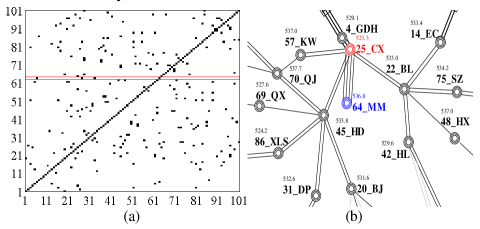
Figure 7: The first-order Chebyshev filter matrix and the reception field of the 64-th station in first-order Chebyshev matrix

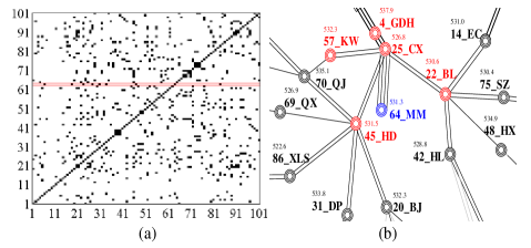
Figure 8: The second Chebyshev filter matrix and the reception field of the 64-th station in second-order Chebyshev matrix

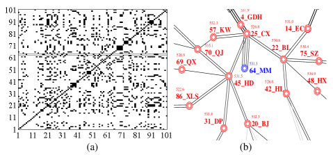
Figure 9: The third-oder Chebyshev filter matrix and the reception field of the 64-th station in third-order Chebyshev matrix

As the reception field of one bus is different according to Chebyshev order, Chebyshev order $K$ can have a certain impact on the performances of STGCN. In this paper, $K$ is set as 2 by multiple tests. Besides, the stacking number of the spatial-temporal information incorporation blocks can also represent the reception field of the buses. To capture the spatial-temporal features from different reception fields, the fusion information from the stacked spatial-temporal information incorporation blocks is utilized for the subsequent SVS assessment.

IV-B3 Spatial-temporal characteristics extraction and node layer representation

The spatial-temporal characteristics of SVS can be extracted by the spatial-temporal information incorporation blocks. Then, in the node layer block, the transformed multi-channel data can be converted into single-channel representation by applying a weighted summation. Before passing data to the system layer, the data are normalized and the absolute values are taken as their node representations.

To illustrate the effectiveness of spatial-temporal information incorporation blocks and node layer representation block, the resulting representations of 400 cases are visualized in Fig. 10 using t-distributed stochastic neighbor embedding (t-SNE) [35], including the data processed by one spatial-temporal information incorporation block $Vidxn_{i,1}$, the data processed by five stacked spatial-temporal information incorporation blocks $Vidxn_{i,5}$, the data processed by spatial-temporal information fusion from the stacked spatial-temporal information incorporation blocks $Vidxz_{i}$, and the data processed by node layer block $Snode_{i}$, $i=1,2,3,...n$. As shown in Fig. 10, after processed by node layer block, stable cases and unstable cases can be distinguished to a large extent with the transformed dataset. It illustrates the effectiveness of spatial-temporal feature extraction and node layer representation block.

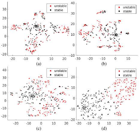
Figure 10: Visualization of the data processed by spatial-temporal information incorporation blocks and node layer block: (a) Data processed by one spatial-temporal information incorporation block; (b) Data processed by five stacked spatial-temporal information incorporation block; (c) Data processed by spatial-temporal information fusion from the stacked spatial-temporal information incorporation blocks; (d) Data processed by node layer block

IV-B4 System layer - identification of the influences of individual buses on SVS

After obtaining the node representations of each case, the simplified differentiable pooling layer is adopted as the system layer. With the node representation and the learned parameters $S$ in the system layer, the SVS status in the target region can be obtained.

The weight values $S$ of the system layer in the well-trained model can indicate the influences of the corresponding stations on SVS related to power plants, reactive power injection and multi-infeed high voltage direct current (HVDC) systems. The values of the learned weights are shown in Fig. 11. The positive/negative weight value indicates the beneficial/detrimental influence of the corresponding station on SVS.

Some stations with negative weights present aggregation behaviors from a spatial perspective, including BA station with the lowest weight value, XD station with the second-lowest weight value, and other stations, CW, ZZ, PC, DF. As shown in Fig. 12, the region corresponding to these stations has multi HVDC systems infeed, including the HVDC system from XR station to BA station and the HVDC system from XS station to DF station. As voltage stability in the multi-HVDC infeed region is prominent due to the interaction between direct current (DC) and alternating current (AC) system, it is consistent with the phenomenon that the stations in that region present negative weights in the system layer.

The stations with the top three highest weights in the system layer correspond to DG, GS, and BJ station. For DG and BJ station, each has a 200 Mvar STATCOM nearby. GS station has three power plants nearby, which are configured with excitation and PSS. It is consistent with the general view that STATCOM and power plants with excitation and PSS can have positive effects on voltage stability, illustrating the effectiveness of the parameters learned in the system layer.

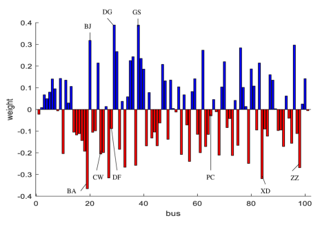
Figure 11: Value of weight in the system layer

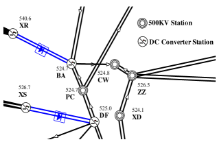
Figure 12: The stations in multi-DC infeed region

IV-C Performance comparison with other existing stability assessment methods

In order to further evaluate the performance of the proposed STGCN, it is compared with the existing methods based on post-fault time series, namely the spatial-temporal shapelet learning method (ST-shapelet) [15], the LSTM-based method [13], and the RVFL-based method [14], under unpredictable faults, noisy environment, topology changes, and different operating points.

The ST-shapelet method, LSTM-based method and RVFL-based method are the typical methods to deal with post-fault time series. The ST-shapelet method first generates voltage animations based on geographical location information and post-fault time series. Then, it utilizes voltage contour in the animations to extract comprehensive spatial-temporal time series. After that, shapelet transform is adopted to convert the time series dataset into a distance dataset. Finally, it employs decision tree to conduct classification. The LSTM-based model is composed of an LSTM layer, a hidden dense neuron layer and a sigmoid function in the end. The LSTM layer contains 128 cells and can be utilized to handle the temporal relationship of the dataset. The hidden neuron layer is used for dimension reduction. After that, the sigmoid function is adopted to normalize the output. RVFL is a randomized learning algorithm in the form of single hidden-layer feedforward network. The post-fault time series are flattened and converted into vectors as the learning input.

IV-C1 Performance comparison of different approaches for SVS assessment under unpredictable faults

With the prepared dataset, the five-fold validation is conducted to compare the performances of different approaches for SVS assessment, and the results are shown in Table I.

As shown in Table I, STGCN has the highest training accuracy and testing accuracy than the other three methods. The decent performances are attributed to the introduction of topology with graph convolution and the carefully designed architecture for SVS assessment. The effectiveness of each part in the proposed network is verified in the previous subsection.

The performances of LSTM and RVFL-based methods are lower than the other two methods. This is because these two methods don’t incorporate any spatial information in their models in any form, while the ST-shapelet method manages to incorporate spatial geographic information into the learning model. However, the spatial information represented by geographic information may not be that suitable compared to introducing topology into the learning model. Therefore, the proposed network shows better performances than the ST-shapelet method.

TABLE I: Performance comparison of different approaches for SVS assessment under unpredictable faults

Model	Training accuracy	Testing accuracy
STGCN (Proposed)	99.4%	98.8%
ST-shapelet	98.1%	98.3%
LSTM	94.8%	94.4%
RVFL	97.7%	97.5%

IV-C2 Performance comparison of different approaches for voltage stability assessment under noisy environment

To test the performances of the proposed STGCN under noisy environment, Gaussian noise is added in the original test dataset. The signal to noise rate (SNR) is set to 45 dB [36]. The performances of different approaches in noisy environments are shown in Table II.

As shown in Table II, STGCN has the highest testing accuracy than the other three methods in noisy environments. This is due to the effective spatial-temporal feature extraction and the introduction of the normalization layer and the dropout layer to the proposed network. As for the ST-shapelet method, it utilizes key subsequence to distinguish the stability of the observed system. Therefore, it is relatively less affected by noise data. The LSTM model doesn’t introduce any module to address noise, which results in poor performance. The RVFL-based method has the worst performance. It is due to its shallow structure. RVFL is in the form of single hidden-layer feedforward network. It cannot extract more effective features than deep learning and is more susceptible to noise.

When the topology of the observed system contains noise, it can have a negative impact on the model performance of STGCN, and the testing accuracy on that occasion is 97.7%. It is still relatively higher than the other three methods, which benefits from the good model design.

TABLE II: Performance comparison of different approaches for SVS assessment in noisy environments

Model	Testing accuracy
STGCN (Proposed)	98.6%
ST-shapelet	97.4%
LSTM	92.0%
RVFL	84.0%

IV-C3 Performance comparison of different approaches for voltage stability assessment under topology changes

To test the performance of the proposed STGCN under topology changes, another 100 cases are generated by setting different topology changes, fault clearing time, and induction motor ratios. These cases consider topology changes in two or three parts. The topology changes are larger than the one-part change in the previous dataset. The performances of different approaches under topology changes are shown in Table III.

As shown in Table III, STGCN has the highest testing accuracy than the other three methods under topology changes. This is because when the topology of the target region changes, it will be reflected in the input topology matrix. Another three methods cannot reveal the changes in topology. The LSTM-based method and RVFL-based method don’t incorporate any spatial information in their models. The ST-shapelet method only utilizes fixed geographic information to extract spatial features.

TABLE III: Performance comparison of different approaches for SVS assessment under topology changes

Model	Testing accuracy
STGCN (Proposed)	96.0%
ST-shapelet	93.0%
LSTM	94.0%
RVFL	93.0%

IV-C4 Performance comparison of different approaches for voltage stability assessment under different operating points

To test the performance of the proposed STGCN under different operating points, another 1500 cases are generated by setting different operating points. Random faults and induction motor ratios are selected in each case. 1200 cases are utilized to retrain the proposed STGCN, and the remaining cases are for testing. The performances of different approaches under different operating points are shown in Table IV.

As shown in Table IV, STGCN has the highest testing accuracy than the other three methods. The decent performance is attributed to two aspects. In the input data aspect, the incorporation of network topology information and the temporal data contains full spatial-temporal dynamics in SVS. In the model aspect, the proposed network is designed according to the SVS characteristics. The performance of the ST-shapelet method is higher than the LSTM method and the RVFL method. This is because the ST-shapelet method manages to incorporate spatial information into the learning model with geographic location information.

TABLE IV: Performance comparison of different approaches for SVS assessment under different operating points

Model	Testing accuracy
STGCN (Proposed)	98.7%
ST-shapelet	97.3%
LSTM	92.0%
RVFL	92.3%

V Conclusion

Short-term voltage instability phenomenon presents spatial-temporal characteristics, but there is currently no systematic approach to incorporate such characteristics into the learning model accurately and effectively. This paper develops STGCN to incorporate the characteristics of SVS into the learning model. It employs Chebyshev graph convolution to integrate topology into the learning model. As Chebyshev filter matrix reveals locality, it is consistent with the spatial characteristics of SVS. Then, the one-dimensional convolution is utilized to extract temporal features. After that, the spatial-temporal features from different reception fields are extracted by the fusion of spatial-temporal information incorporation blocks. Finally, the node layer and system layer are designed to provide the final assessment result. Test results on Guangdong Power Grid illustrate that compared with the existing typical methods, the proposed STGCN can achieve higher model accuracy, better robustness in noisy environments, and better adaptability to topology changes and different operating points. Besides, parameters of the system layer in the well-trained stability assessment model can provide valuable information about the influences of individual buses on SVS.

References

- [1] T. V. Cutsem and C. Vournas, Voltage Stability of Electric Power Systems. Norwell, MA, USA: Kluwer, 1998.
- [2] AEMO. (2016) Preliminary report-black system event in south australia on 28 september 2016. [Online]. Available: https://www.aemo.com.au/Media-Centre/-/media/BE174B1732CB4B3ABB74BD507664B270.ashx
- [3] K. E. Martin, “Synchrophasor Measurements Under the IEEE Standard C37.118.1-2011 With Amendment C37.118.1a,” IEEE Transactions on Power Delivery, vol. 30, no. 3, pp. 1514-1522, 2015.
- [4] NERC/WECC Planning Standards [Online]. Available: https://www.wecc.biz/library/Library/Planning%20Committee%20Handbook/WECC-NERC%20Planning%20Standards.pdf
- [5] Z. Liu, “Voltage stability and preventive control in China,” in Proc. IFAC Symp. Power Plants and Power Systems Control, Seoul, Korea, 2003.
- [6] S. Dasgupta, M. Paramasivam, U. Vaidya, and V. Ajjarapu, “Real-time monitoring of short-term voltage stability using pmu data,” IEEE Transactions on Power Systems, vol. 28, no. 4, pp. 3702–3711, 2013.
- [7] Y. Dong, X. Xie, K. Wang, B. Zhou, and Q. Jiang, “An Emergency-Demand-Response Based Under Speed Load Shedding Scheme to Improve Short-Term Voltage Stability,” IEEE Transactions on Power Systems, vol. 32, pp. 3726–3735, 2017.
- [8] D. Q. Zhou, U. D. Annakkage, and A. D. Rajapakse, “Online monitoring of voltage stability margin using an artificial neural network,” IEEE Trans. Power Syst., vol. 25, no. 3, pp. 1566–1574, 2010.
- [9] Y. Xu, R. Zhang, J. Zhao, Z. Y. Dong, D. Wang, H. Yang, and K. P. Wong, “Assessing short-term voltage stability of electric power systems by a hierarchical intelligent system,” IEEE Trans. Neural Networks Learn. Syst., vol. 27, no. 8, pp. 1686–1696, 2016.
- [10] Y. Zhang, Y. Xu, Z. Y. Dong, and R. Zhang, “A hierarchical self-adaptive data-analytics method for real-time power system short-term voltage stability assessment,” IEEE Transactions on Industrial Informatics, vol. 15, no. 1, pp. 74–84, 2019.
- [11] L. Zhu, C. Lu, and Y. Sun, “Time series shapelet classification based online short-term voltage stability assessment,” IEEE Transactions on Power Systems, vol. 31, no. 2, pp. 1430–1439, 2016.
- [12] L. Zhu, C. Lu, Z. Y. Dong, and C. Hong, “Imbalance learning machine-based power system short-term voltage stability assessment,” IEEE Transactions on Industrial Informatics, vol. 13, no. 5, pp. 2533–2543, 2017.
- [13] J. J. Q. Yu, D. J. Hill, A. Y. S. Lam, J. Gu, and V. O. K. Li, “Intelligent time-adaptive transient stability assessment system,” IEEE Transactions on Power Systems, vol. 33, no. 1, pp. 1049–1058, 2018.
- [14] Y. Zhang, Y. Xu, R. Zhang, and Z. Y. Dong, “A missing-data tolerant method for data-driven short-term voltage stability assessment of power systems,” IEEE Transactions on Smart Grid, vol. 10, no. 5, pp. 5663–5674, 2019.
- [15] L. Zhu, C. Lu, I. Kamwa, and H. Zeng, “Spatial–temporal feature learning in smart grids: A case study on short-term voltage stability assessment,” IEEE Transactions on Industrial Informatics, vol. 16, no. 3, pp. 1470–1482, 2020.
- [16] K. Chen, J. Hu, Y. Zhang, Z. Yu, and J. He, “Fault location in power distribution systems via deep graph convolutional networks,” IEEE Journal on Selected Areas in Communications, vol. 38, no. 1, pp. 119–131, 2020.
- [17] P. W. Battaglia, J. B. Hamrick, V. Bapst, A. Sanchezgonzalez, V. Zambaldi, M. Malinowski, A. Tacchetti, D. Raposo, A. Santoro, R. Faulkner et al., “Relational inductive biases, deep learning, and graph networks,” arXiv: Learning, 2018.
- [18] Z. Wu, S. Pan, F. Chen, G. Long, C. Zhang, and P. S. Yu, “A comprehensive survey on graph neural networks,” arXiv: Learning, 2019.
- [19] B. Yu, H. Yin, and Z. Zhu, “Spatio-temporal graph convolutional networks: A deep learning framework for traffic forecasting,” in Proceedings of the Twenty-Seventh International Joint Conference on Artificial Intelligence, IJCAI, 2018, pp. 3634–3640.
- [20] H. Yao, F. Wu, J. Ke, X. Tang, Y. Jia, S. Lu, P. Gong, J. Ye, and Z. Li, “Deep multi-view spatial-temporal network for taxi demand prediction.” arXiv: Learning, 2018.
- [21] Y. Seo, M. Defferrard, P. Vandergheynst, and X. Bresson, “Structured sequence modeling with graph convolutional recurrent networks,” arXiv: Machine Learning, 2016.
- [22] S. Yan, Y. Xiong, and D. Lin, “Spatial temporal graph convolutional networks for skeleton-based action recognition,” in Proceedings of the Thirty-Second AAAI Conference on Artificial Intelligence, (AAAI-18), 2018, pp. 7444–7452.
- [23] R. Ying, J. You, C. Morris, X. Ren, W. L. Hamilton, and J. Leskovec, “Hierarchical graph representation learning with differentiable pooling,” arXiv: Learning, 2018.
- [24] J. D. Weber and T. J. Overbye, “Voltage contours for power system visualization,” IEEE Transactions on Power Systems, vol. 15, no. 1, pp. 404–409, 2000.
- [25] J. Bruna, W. Zaremba, A. Szlam, and Y. Lecun, “Spectral networks and locally connected networks on graphs,” arXiv: Learning, 2013.
- [26] M. Defferrard, X. Bresson, and P. Vandergheynst, “Convolutional neural networks on graphs with fast localized spectral filtering,” in Advances in Neural Information Processing Systems, 2016, pp. 3837–3845.
- [27] T. Kipf and M. Welling, “Semi-supervised classification with graph convolutional networks,” arXiv: Learning, 2016.
- [28] F. Scarselli, M. Gori, A. C. Tsoi, M. Hagenbuchner, and G. Monfardini, “The graph neural network model,” IEEE Transactions on Neural Networks, vol. 20, no. 1, pp. 61–80, 2009.
- [29] J. Gilmer, S. S. Schoenholz, P. F. Riley, O. Vinyals, and G. E. Dahl, “Neural message passing for quantum chemistry,” in Proceedings of the 34th International Conference on Machine Learning, ICML, vol. 70, 2017, pp. 1263–1272.
- [30] W. L. Hamilton, Z. Ying, and J. Leskovec, “Inductive representation learning on large graphs,” in Advances in Neural Information Processing Systems, 2017, pp. 1024–1034.
- [31] D. Kinga and J. B. Adam, “A method for stochastic optimization,” in International Conference on Learning Representations (ICLR), 2015.
- [32] Y. N. Dauphin, A. Fan, M. Auli, and D. Grangier, “Language modeling with gated convolutional networks,“ in International Conference on Machine Learning (ICLR), 2017, pp. 933-941.
- [33] A. Krizhevsky, I. Sutskever, G. E. Hinton, “ImageNet Classification with Deep Convolutional Neural Networks,” in neural information processing systems, 2012.
- [34] M. D, Zeiler, and R. Fergus, “Visualizing and Understanding Convolutional Networks,” in european conference on computer vision, 2014.
- [35] L. V. Der Maaten and G. E. Hinton, “Visualizing data using t-sne,” Journal of Machine Learning Research, vol. 9, pp. 2579–2605, 2008.
- [36] M. G. Brown, M. Biswal, S. Brahma, S. J. Ranade, and H. Cao, “Characterizing and quantifying noise in pmu data,” in IEEE Power and Energy Society General Meeting, 2016, pp. 1–5.