Exploring the representativeness of the M5 competition data

Abstract

The main objective of the M5 competition, which focused on forecasting the hierarchical unit sales of Walmart, was to evaluate the accuracy and uncertainty of forecasting methods in the field in order to identify best practices and highlight their practical implications. However, whether the findings of the M5 competition can be generalized and exploited by retail firms to better support their decisions and operation depends on the extent to which the M5 data is sufficiently similar to unit sales data of retailers that operate in different regions, sell different types of products, and consider different marketing strategies. To answer this question, we analyze the characteristics of the M5 time series and compare them with those of two grocery retailers, namely Corporación Favorita and a major Greek supermarket chain, using feature spaces. Our results suggest that there are only small discrepancies between the examined data sets, supporting the representativeness of the M5 data.

1 Introduction

Time series forecasting competitions provide valuable insights when it comes to identifying the most appropriate methods for producing point or probabilistic forecasts for a forecasting task under investigation, with their findings having several implications, both for the industry and the academia (Hyndman, 2020). This is especially true when the time series data considered by the competitions and the forecasting methods originally submitted are publicly available to use, enabling the replication of their results (Makridakis et al., 2018). This was the case with M5, which focused on forecasting the hierarchical unit sales of the largest retail company in the world, Walmart (Makridakis et al., 2020a).

The results of the M5 competition demonstrate that there is still room for improving forecasting accuracy and uncertainty estimation in the retail industry. Similar to M4 (Makridakis et al., 2020c), traditional statistical methods, widely used by retailers for supporting decisions related to supply chain management, were outperformed by state-of-the-art machine learning ones, with the improvements reported for the winning submissions over the top-performing benchmarks being higher than 20% according to the competition’s evaluation measures. This finding indicates that retail and logistic firms could benefit significantly from utilizing the winning submissions of the competition, especially if we consider that small improvements in accuracy can lead to considerable inventory reductions (Syntetos et al., 2010), while slight inaccuracies to higher stock holdings and lower service levels (Ghobbar & Friend, 2003; Pooya et al., 2019).

However, the practical implications of forecasting competitions have been widely criticized by the forecasting community and especially its practitioners, claiming that the findings reported may depend on the particularities of the data set used for conducting the competition, thus being difficult to generalize and exploit in business, real-life applications (Ord, 2001; Clements & Hendry, 2001; Armstrong & Green, 2019; Darin & Stellwagen, 2019; Fry & Brundage, 2019; Bojer & Meldgaard, 2021). For example, M5 focused on the sales of ten indicative US stores of a global retail firm located in three states (California, Wisconsin, and Texas), covering the period from 2011 to 2016 and three product categories (“Foods”, “Household”, and “Hobbies”). Therefore, it could be the case that its results are not representative of a retail firm operating in South America in the same period or another retailer operating in Greece in a different period. Indeed, the country of origin of the data may affect the characteristics of the series, especially if the types of the products sold and the marketing strategies considered (e.g., discounts and promotions) differ (Makridakis et al., 2021). Moreover, as COVID-19 has recently proved, the period of analysis may highly affect the patterns of the data and, as a result, the appropriateness of the forecasting methods that should be employed for producing accurate forecasts (Wang et al., 2020; Panzone et al., 2021; Güngör et al., 2021).

As the literature suggests, no single method is suitable for all forecasting tasks (Lawrence, 2001) and, therefore, identifying “horses for courses” (Petropoulos et al., 2014) is essential. This was also true in the M5 competition where depending on the nature of the series, the cross-sectional level being forecast, and the quantile considered for estimating uncertainty, different methods were found to be the top-performing ones (Makridakis et al., 2020d, e). It becomes evident that although the winning method of a competition may not always outperform the rest of the available alternatives in all subsets of the competition’s data set, its findings can still be useful when forecasters are able to identify and select the methods that performed best in a subset of series which represent their own data set adequately, thus fitting their forecasting needs (Fildes, 2020; Makridakis et al., 2020b). Drawing from the above, evaluating the extent to which the M5 data reflects the particularities of various retail firms becomes critical.

In this discussion paper, we try to answer this question by analyzing the time series features of the M5 data set and comparing them with those of two other retail firms, namely Corporación Favorita, a major grocery retailer in South America, and a major supermarket chain in Greece. We base our analysis on feature space visualizations, as proposed by (Kang et al., 2020), and consider intuitive measures of coverage and miscoverage to quantify our results.

We should clarify that our analysis focuses on the sales data itself, ignoring the explanatory variables that typically accompany such data to enhance forecasting performance (Fildes et al., 2019). Therefore, the representatives of the M5 data set is evaluated based on the patterns that the M5 sales data display per se compared to that of other retail firms and not in terms of the external information that may be available to forecasters to help them explain data variations or determine changes in their future behavior. For instance, the M5 data set included information about special days and holidays, selling prices, and promotion activities. Although access in that kind of information may be typical in retail sales forecasting applications, other data sets may be richer in terms of explanatory variables, including also information about future weather conditions, product reviews, trends, and fuel prices, among others (Ma & Fildes, 2021).

2 Time series feature extraction and selection

Time series feature representation approaches allow the extensive investigation and intuitive visualization of large data sets. Several studies have exploited feature-based time series instance space analysis to explore previous forecasting competition data sets (e.g., Kang et al., 2017; Spiliotis et al., 2020; Li et al., 2020). However, a significant difference of M5 over previous forecasting competitions is that it involved intermittent demand series that display zeros and irregular patterns. In this respect, in this study, feature extraction and selection are performed using a methodological approach tailored for the examined application, as presented in the remainder of this section.

2.1 Feature extraction

2.1.1 Determining the pool of features

Feature extraction begins by constructing a pool of features $\mathcal{F}$, specifically by concatenating two sets of time series features, namely $\mathcal{F}_{\text{tsfresh}}$, from the tsfresh module for python (Christ et al., 2018), and $\mathcal{F}_{\text{tsfeatures}}$, from the tsfeatures package for R (Hyndman et al., 2020). In total, $\mathcal{F}$ consists of $P=836$ features, computed for all the series under examination. The tsfresh package involves a variety of features, such as basic time series statistics, correlation measures, entropy estimations, and coefficients of standard time series forecasting and analysis methods. On the other hand, the tsfeatures package includes statistics that are computed on the first and second-order differences of the raw series, account for seasonality, and exploit the outputs of popular time series decomposition methods, among others.

2.1.2 Expanding the pool of features for higher temporal aggregation levels

Due to the intermittency of typical retail sales series, some features like seasonality and trend may be observed only at higher temporal aggregation levels. Moreover, the values of the features may change considerably across different frequencies (Kourentzes et al., 2014). To that end, we expand the initial pool of features $\mathcal{F}$, originally computed for daily sales data, by performing temporal aggregation and calculating their values on a weekly and monthly level as well. In this regard, the final pool of features examined consists of a total of $3\cdot P=2508$ features per series.

2.2 Feature selection

After removing those with missing or unique values, 1654 features are kept. Given the large number of features, which greatly increases the dimensionality and complexity of the analysis, we employ a feature selection procedure by tailoring the approach proposed by Lubba et al. (2019) to meet our requirements. The feature selection procedure involves three steps, namely statistical pre-filtering, performance evaluation, and redundancy minimization, as described in the following subsections.

2.2.1 Statistical pre-filtering

The statistical pre-filtering step aims to remove the non-significant features rather than choosing the most meaningful ones. It involves the $z$-score standardization of the features and eliminating those that display the same or similar values across different series. To that end, we first select the features that can effectively differentiate distinct classes in the M5 data set in a statistically significant manner, considering four different item classification tasks in terms of states (three classes), stores (ten classes), product categories (three classes), and product departments (seven classes).

For each feature, we perform the nonparametric Kruskal-Wallis hypothesis test (Kruskal & Wallis, 1952) to each of the four classification tasks, thus obtaining four $p$-values per feature accordingly. Note that, in contrast to the Analysis of Variance (ANOVA) method, the Kruskal-Wallis hypothesis test does not assume normally distributed populations, also performing better when population asymmetries are present (Hecke, 2012). We combine the four $p$-values as one single overall test for each feature using the Fisher’s method (Fisher, 1925). According to Fisher’s method, $k$ independent $p$-values can be combined into one statistic that follows a $\chi^{2}$ distribution with $2\cdot k$ degrees of freedom:

$$X=-2\sum_{i=1}^{k}\ln{p_{i}}\sim\chi^{2}(2\cdot k),$$ (1)

where $p_{i}$ denotes the $p$-value for the $i$^th ($i=1,\cdots,k$) statistical test (i.e., the $i$^th classification task in our case) and $k$ is the number of tests. The combined $p$-value for each feature can be obtained according to Equation (1). Finally, we apply the Holm-Bonferroni method (Holm, 1979) to correct the newly constructed $p$-value and reduce the type I errors of the hypothesis tests for the specified significance level, which may be caused due to the large number of tests involved in the process. To do so, we first sort all the $p$-values in ascending order and obtain their ranks. Then, we compare the original $p$-values with the corrected values $p/(n+1-\text{rank}(p))$, where $n$ represents the total number of features. The comparison continues until some original $p$-value is larger than the corresponding corrected $p$-value. Eventually, the features with smaller original $p$-values than the corrected ones at the stop point are retained. In this step, 132 of 1654 features are dropped with a significance level of 0.05.

2.2.2 Performance evaluation

In order to evaluate the quality of the extracted features, we employ the Regressional ReliefF (RReliefF) algorithm (Robnik-Šikonja & Kononenko, 2003), which is an extension of the ReliefF algorithm for regression problems (Kononenko, 1994). ReliefF is a robust filtering method used to select features in multi-class classification problems, with the basic idea of identifying feature differences between nearest instance pairs. Specifically, ReliefF calculates a score $W_{F}$ for each feature $F$ and performs feature selection accordingly. According to Kononenko (1994), the $W_{F}$ scores derived by ReliefF are approximations of the following difference of probabilities:

$$W_{F}= p(\text{different~{}values~{}of}~{}F|\text{nearest~{}instances~{}from~{}a~{}different~{}class})-$$ (2)

$$p(\text{different~{}values~{}of}~{}F|\text{nearest~{}instances~{}from~{}the~{}same~{}class}).$$

Similarly, RReliefF calculates the probability of the predictions of two instances being different from each other. Based on Bayes’ rule and Equation (2), $W_{F}$ can be computed as follows

$$W_{F}=\frac{p_{\text{diffP}|\text{diffF}}\cdot p_{\text{diffF}}}{p_{\text{diffP}}}-\frac{(1-p_{\text{diffP}|\text{diffF}})\cdot p_{\text{diffF}}}{1-p_{\text{diffP}}},$$ (3)

where

$$p_{\text{diffF}}= p(\text{different~{}value~{}of}~{}F|\text{nearest~{}instances}),$$ (4)

$$p_{\text{diffP}}= p(\text{different~{}predictions}|\text{nearest~{}instances}),$$

$$p_{\text{diffP}|\text{diffF}}= p(\text{different~{}predictions}|\text{different~{}values~{}of}~{}F~{}\text{and~{}nearest~{}instances}).$$

In our case, seven point forecasts are used as predictions to evaluate the quality of the features more moderately, meaning that seven $W_{F}$ scores are computed for each feature. These scores are then combined into single quality vectors and used as input to the following step of the procedure to support further feature selection. For more details on the RReliefF algorithm and $W_{F}$ score estimation, please refer to the study of Robnik-Šikonja & Kononenko (2003).

2.2.3 Redundancy minimization

We employ hierarchical clustering to reduce the redundancy in the obtained top-performing features using the Pearson correlation distance (cosine distance) with complete linkage at a threshold of 0.2 (Lubba et al., 2019), which makes the pairwise correlation coefficients of the features in the same cluster larger than 0.8, thus forming clusters of similarly performing features. To do so, we use the vectors generated from the previous step (performance evaluation) as input to the clustering method. In each cluster, the feature with the largest mean quality score is selected.

2.2.4 Selected features

After completing the feature selection procedure, we end up with a total of 42 features, in which 10 features are computed at a daily level, while 22 and 10 at a weekly and monthly level, respectively. That reflects the benefits of considering temporal aggregation for extracting more meaningful and descriptive features. More details of the selected features $\mathcal{F}^{*}$ (including their names, description, packages employed, and temporal aggregation levels considered) are summarized in the supplementary material of the paper. It is evident that $\mathcal{F}^{*}$ involves a wide range of time series features, including information about the coefficients of the discrete Fourier transform, the location of the observations of the series, the variance and distribution of the data, the differential characteristics of the series, the entropy and linear trend of the series, the intermittency, and the statistics of popular time series analysis tests, among others.

We should clarify that although some of the selected features may be challenging to interpret, our approach is still preferable over alternative ones that arbitrarily consider a limited sample of features, being more flexible and generic. This becomes evident if we consider that the selection of proper features depend strongly on the nature and the context of the application. Hence, automatic ways of feature selection have attracted much attention in the forecasting community (e.g., Li et al., 2020).

3 Representativeness of the M5 competition data

To evaluate the extent of the differences observed between the series of the M5 competition and those of other retail firms, we tried to retrieve data sets of retail companies that operate in different regions, consider different marketing strategies, and sell different types of products. Moreover, we tried to identify data sets that cover different operation periods than the one examined in M5 to account for possible changes in customer behavior, trends, and special events.

To that end, we considered the data sets available in the online data science platform of Kaggle, used in past forecasting competitions (Bojer & Meldgaard, 2021). Although there is a large number of competition data sets available, most of them are not comparable to M5 as they involve series monitored at different temporal aggregation levels, refer to different industries and applications, or originate from the same retail firm (Walmart). This limited our choices to the data set used for conducting the “Corporación Favorita Grocery Sales Forecasting” competition, involving the daily unit sales of a major grocery retail firm in South America. The data (174,654 series) is provided at product-store level, as done in M5, and covers a period of about 1,114 days, ranging from January 2013 to August 2017, which overlaps to some extent with the period considered in M5. Moreover, the data set involves 16 states, 54 stores, and 33 product categories.

In addition to the Corporación Favorita data set, we were able to acquire another one, generously provided to us by a major Greek supermarket chain, involving the daily unit sales of various products sold at 227 stores located all over Greece across 80 product categories. The data (7,248 series) is provided at warehouse level and covers a period of about 748 days, ranging from April 2018 to May 2020. Note that this period does not overlap with the one considered in M5, accounting also for the first wave of the COVID-19 outbreak and the respective lockdown effect. Note also that, similar to Corporación Favorita, the Greek retail firm drives its sales through promotions and discounts, in contrast to Walmart, which adopts a constant low-price marketing strategy. The aggregated unit sales of the examined data sets are presented in Figure 1. Observe that the sales of the M5 and Corporación Favorita data set are characterized by greater trend compared to the Greek retailer, with those of Corporación Favorita being also more volatile. Moreover, the stores of the Greek retailer are closed on most Sundays, in contrast to those of the other two firms that are closed only on Christmas. However, as shown in Figure 1, this is not the case in all weeks. Thus, Sundays were not removed from the Greek retailer’s data and the selected time series features were calculated for all data sets in a consistent fashion, assuming a frequency of seven.

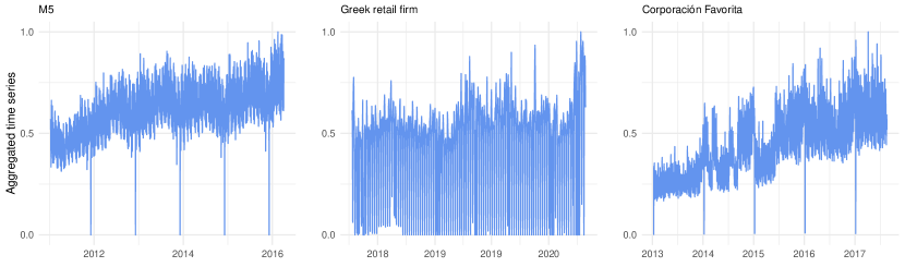
Figure 1: Aggregated unit sales of the examined data sets: M5 competition (Walmart), Greek supermarket chain, and Corporación Favorita. Sales are normalized using min-max scaling to facilitate comparisons.

Apart from covering different regions, time periods, product categories, and marketing strategies, the series of the three data sets considered also display major differences in terms of intermittency (average inter-demand interval) and demand size erraticness (Syntetos & Boylan, 2005). As shown in Table 1, the majority of the M5 time series are intermittent, while most of the series of the Greek firm and Corporación Favorita are lumpy. However, in the latter case, the population of the four time series categories is far more balanced compared to the rest. These insights further motivate our research question, stressing the necessity to assess the representativeness of the M5 series in terms of feature spaces. Figure A of the supplementary material provides also useful visualizations regarding the distribution of the values of the selected features across the time series of the examined data sets.

Table 1: Overview of the examined data sets. For each data set, the region and period of operation are reported, along with the number of series involved and their average lengths. The percentages of erratic, lumpy, smooth, and intermittent series in each data set are also reported.

Data set	Region	Period	Observations	Time series	Erratic	Lumpy	Smooth	Intermittent
M5 (Walmart)	USA	Jan 2011 - Apr 2016	1,507	30,490	2.88%	17.01%	6.76%	73.35%
Greek retail firm	Greece	Apr 2018 - May 2020	748	7,248	18.10%	41.75%	10.58%	29.57%
Corporación Favorita	Ecuador	Jan 2013 - Aug 2017	1114	174,654	20.65%	30.91%	23.07%	25.37%

In order to visualize the discrepancies between the three data sets, we employ the approach proposed by Kang et al. (2020) which utilizes the t-Stochastic Neighbor Embedding (t-SNE, Van der Maaten & Hinton, 2008) to create feature spaces. Note that t-SNE is more effective than its linear counterparts (e.g., PCA, Principal Component Analysis) when considering multiple features that are correlated in a nonlinear fashion, placing similar data points close together while also keeping dissimilar ones far apart. While performing t-SNE, we use PCA to initialize the embedding, since informative initialization is more globally stable than random initialization in t-SNE (Kobak & Linderman, 2021). The generated feature spaces are presented in Figure 2. We observe that the series of the M5 competition successfully fill the overall instance space defined by the three retail firms, despite the fact that each data set displays different regions of higher densities. The same conclusion is drawn by observing the ranges and shapes of the distributions of the first and second t-SNE dimensions of the three data sets.

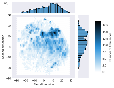
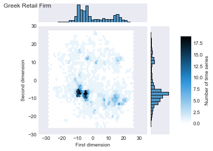
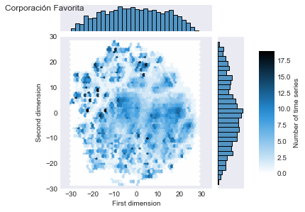
Figure 2: The two-dimensional t-SNE instance spaces of the M5 (Walmart), Greek retail firm, and Corporación Favorita data sets.

In order to quantify the differences and similarities observed among the three data sets, we proceed by computing the following measures:

• the miscoverage of data set A over data set B (Kang et al., 2020):

  $$miscoverage_{A/B}=N^{-2}\displaystyle\sum_{i=1}^{N^{2}}(1-I_{i,A})\times I_{i,B},$$

  where $N^{2}=900$ is the number of squares of the grid superimposed on the overall space and $I_{i,A}$ equals to one if points in data set A fall within the $i^{th}$ square, being zero otherwise. An analogous definition is applied to $I_{i,B}$ computed based on data set B.

• the percentage of points of data set A that lie within the space where data set B is not encountered (non-overlapping ratio):

  $$NOR_{A/B}=\frac{\displaystyle\sum_{i=1}^{N^{2}}n_{i,A}\times(1-I_{i,B})}{\displaystyle\sum_{i=1}^{N^{2}}n_{i,A}},$$

  where $n_{i,A}$ is the number of points of the data set A that fall within the $i^{th}$ square.

These measures can effectively quantify both the spatial discrepancy of the feature spaces and the significance of that discrepancy in an intuitive way. Note however that this is true if we assume that the existence of a single series per square is adequate to indicate representativeness. The values of the two measures are summarized in Table 2. As seen, although in 5.56% of the feature space defined by Corporación Favorita and M5 there is at least one time series of the former data set but none of the latter, this part of space accounts for just 2.48% of the overall series included in the Corporación Favorita data. Similarly, only 0.67% of the space defined by the Greek retail firm and M5 is not represented by the latter, accounting for 0.37% of the series of the Greek retailer.

Table 2: Pairwise miscoverage and non-overlapping ratios among the data sets of the M5 competition (Walmart), the Greek retail firm, and Corporación Favorita.

Data set A	Data set B
	M5	Greek retail firm	Corporación Favorita
	Pairwise miscoverage
M5 (Walmart)	-	0.67%	5.56%
Greek retail firm	18.78%	-	23.56%
Corporación Favorita	0.11%	0.00%	-
	Pairwise non-overlapping ratio
M5 (Walmart)	-	14.70%	0.02%
Greek retail firm	0.37%	-	0.00%
Corporación Favorita	2.48%	24.23%	-

Based on our results, we conclude that there are only small discrepancies between the examined data sets and that the findings of M5 can be relevant for various retail firms. Moreover, we find that although the size of the data set affects to some extent the degree of representativeness, M5 manages to effectively cover the feature space of the Corporación Favorita data, which consists of about 5.7 times more series and considerably more stores, locations, and product categories. Moreover, we find that the degree of miscoverage is not affected by the period examined, even when special events like the COVID-19 outbreak are present. This result reflects the diversity of the products and locations considered for constructing the M5 data set, as well as the representativeness of the period examined, accounting both for typical, business-as-usual days and special ones.

To further validate our conclusions, we conduct a similar but simpler analysis that considers the six intuitive time series features proposed by Kang et al. (2017) (spectral entropy, strength of trend, strength of seasonality, seasonal period, first order autocorrelation, and optimal Box-Cox transformation parameter), plus two additional ones that can effectively capture intermittency (average inter-demand interval) and erraticness (squared coefficient of variation). Thus, we end up with eight primary features, each computed at a daily, weekly, and monthly level, resulting in a set of 24 features in total. After computing the values of these features for all the time series of the data sets, we apply a principal component analysis and use the first two components to project the series onto a 2-dimensional space to allow for interpretable data visualizations. The resulting graphs of this approach, shown in Figure B of the supplementary material of the paper, lead to similar findings with the previous approach in the sense that only small discrepancies can be identified between the three data sets examined.

4 Conclusion

In this study, we extended previous work done in feature-based time series instance space analysis, incorporating a plethora of features computed across multiple temporal aggregation levels and using an intuitive feature selection process to capture the key features of the M5 competition data set and evaluate the degree of its representativeness for the retail industry. To do so, we considered two additional retail sales data sets that cover different regions, time periods, product categories, and marketing strategies compared to M5.

Our analysis has found no meaningful inconsistencies between the M5 data and the series of the two other grocery retailers, with any discrepancies observed between the examined data sets being minor. This was also true when data sets of significantly larger size and diversity in terms of stores, locations, and product categories were considered, as well as when different time periods were examined. However, we should note that our analysis is limited to companies that sell their products through brick-and-mortar stores, with a particular focus on groceries. As such, it could be the case that online retailers and firms that sell different types of products, such as pharmaceutical and technological ones, may experience different sales patterns. In addition, our analysis focuses on the sales data itself, thus ignoring the representativeness of the explanatory variables that typically accompany this data to enhance forecasting performance.

Supplementary material

Table 3: *

Table A: Description of the 42 time series features selected ($\mathcal{F}^{*}$) for conducting the analysis. D (daily), W (weekly), and M (monthly) indicate the temporal aggregation level at which the features are computed. The software package used for the estimation of the features is also provided.
No.	Feature	Description	Package	D	W	M
1	count_below_t_0	the percentage of observations in the series that are lower than or equal to zero	tsfresh	✓	-	-
2	fft_coefficient_attr_angle_coeff_63	the angle of the 63rd coefficient of the discrete Fourier transform	tsfresh	✓	-	-
3	trough	trough	tsfeatures	✓	-	-
4	fft_coefficient_attr_angle_coeff_73	the angle of the 73rd coefficient of the discrete Fourier transform	tsfresh	✓	-	-
5	has_duplicate_max	Boolean variable denoting whether the maximum value of the series is observed more than once	tsfresh	✓	-	-
6 & 7	fft_coefficient_attr_angle_coeff_1	the angle of the 1st coefficient of the discrete Fourier transform	tsfresh	✓	-	✓
8	fft_coefficient_attr_angle_coeff_22	the angle of the 22nd coefficient of the discrete Fourier transform	tsfresh	✓	-	-
9	fft_coefficient_attr_angle_coeff_59	the angle of the 59th coefficient of the discrete Fourier transform	tsfresh	✓	-	-
10	variance_larger_than_standard_deviation	Boolean variable denoting whether the variance of the series is greater than its standard deviation	tsfresh	✓	-	-
11 & 12	fft_coefficient_attr_angle_coeff_26	the angle of the 26th coefficient of the discrete Fourier transform	tsfresh	✓	✓	-
13	augmented_dickey_fuller_attr_teststat_autolag_AIC	the statistic of the ADF test where the lag is chosen by AIC	tsfresh	-	✓	-
14	change_quantiles_mean_isabs_True_ qh_1.0_ql_0.8	the mean, absolute value of consecutive changes of the series inside the corridor determined by the quantiles 0.8 and 1 of its distribution	tsfresh	-	✓	-
15	fft_coefficient_attr_imag_coeff_47	the imaginary part of the 47th coefficient of the discrete Fourier transform	tsfresh	-	✓	-
16	fft_coefficient_attr_real_coeff_36	the real part of the 36th coefficient of the discrete Fourier transform	tsfresh	-	✓	-
17	number_crossing_m_1	the number of crossings of series on 1	tsfresh	-	✓	-
18 & 19	fft_coefficient_attr_angle_coeff_2	the angle of the 2nd coefficient of the discrete Fourier transform	tsfresh	-	✓	✓
20	fft_coefficient_attr_angle_coeff_5	the angle of the 5th coefficient of the discrete Fourier transform	tsfresh	-	✓	-
21	fft_coefficient_attr_imag_coeff_44	the imaginary part of the 44th coefficient of the discrete Fourier transform	tsfresh	-	✓	-
22	cwt_coefficients_coeff_12w_2_widths_(2, 5, 10, 20)	the 12th coefficient of the continuous wavelet transform for the Ricker wavelet	tsfresh	-	✓	-
23	fft_coefficient_attr_real_coeff_38	the real part of the 38th coefficient of the discrete Fourier transform	tsfresh	-	✓	-
24	fft_coefficient_attr_real_coeff_42	the real part of the 42nd coefficient of the discrete Fourier transform	tsfresh	-	✓	-
25	fft_coefficient_attr_angle_coeff_20	the angle of the 20th coefficient of the discrete Fourier transform	tsfresh	-	✓	-
26	fft_coefficient_attr_imag_coeff_49	the imaginary part of the 49th coefficient of the discrete Fourier transform	tsfresh	-	✓	-
27	agg_linear_trend_attr_rvalue_ chunk_len_10_f_agg_var	the r value of a linear regression with chunks for time series that were aggregated over chunks by variance	tsfresh	-	✓	-
28	fft_coefficient_attr_real_coeff_45	the real part of the 45th coefficient of the discrete Fourier transform	tsfresh	-	✓	-
29	fft_coefficient_attr_real_coeff_46	the real part of the 46th coefficient of the discrete Fourier transform	tsfresh	-	✓	-
30	fft_coefficient_attr_imag_coeff_46	the imaginary part of the 46th coefficient of the discrete Fourier transform	tsfresh	-	✓	-
31	fft_coefficient_attr_abs_coeff_49	the absolute value of the 49th coefficient of the discrete Fourier transform	tsfresh	-	✓	-
32	approximate_entropy_m_2_r_0.5	approximate entropy	tsfresh	-	✓	-
33	fft_coefficient_attr_real_coeff_43	the real part of the 43rd coefficient of the discrete Fourier transform	tsfresh	-	✓	-
34	fft_coefficient_attr_real_coeff_48	the real part of the 48rd coefficient of the discrete Fourier transform	tsfresh	-	✓	-
35	fourier_entropy_bins_5	fourier entropy considering bins of 5 observations	tsfresh	-	-	✓
36	change_quantiles_mean_isabs_True_ qh_0.4_ql_0.2	the mean, absolute value of consecutive changes of the series inside the corridor determined by the quantiles 0.2 and 0.4 of its distribution	tsfresh	-	-	✓
37	ratio_beyond_r_sigma_r_1	the ratio of values that are over $r\cdot\sigma$ away from the mean of the series	tsfresh	-	-	✓
38	e_acf1	the first autocorrelation coefficient of the remainder of the STL decomposition	tsfeatures	-	-	✓
39	change_quantiles_var_isabs_False_qh_ 0.4_ql_0.2	the variance of consecutive changes of the series inside the corridor determined by the quantiles 0.2 and 0.4 of its distribution	tsfresh	-	-	✓
40	change_quantiles_var_isabs_False_qh_ 0.6_ql_0.4	the variance of consecutive changes of the series inside the corridor determined by the quantiles 0.4 and 0.6 of its distribution	tsfresh	-	-	✓
41	large_standard_deviation_r_0.3	Boolean variable denoting whether the deviation of the series is higher than 0.3 times the range of the series	tsfresh	-	-	✓
42	agg_linear_trend_attr_rvalue_chunk_ len_5_ f_agg_max	the r value of a linear regression with chunks for time series that were aggregated over chunks by maximum	tsfresh	-	-	✓

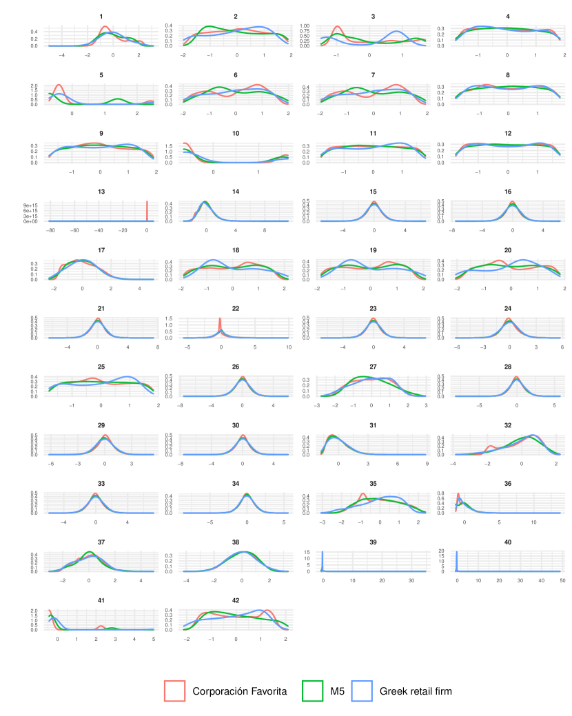
Figure A: Distributions of the 42 time series features selected ($\mathcal{F}^{*}$) for conducting the analysis compared among the three examined data sets. The title of each plot indicates the number of each feature, as shown in Table A.

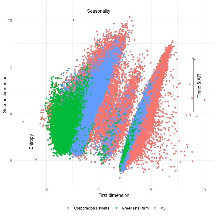
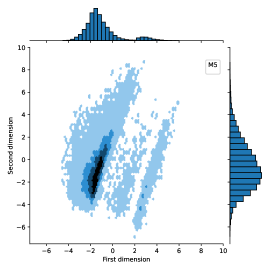
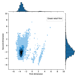
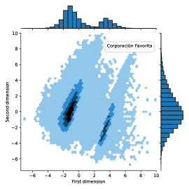
Figure B: Instance spaces of the M5 (Walmart), Greek retail firm, and Corporación Favorita data sets using the 6 series features proposed by Kang et al. (2017), average inter-demand interval and squared coefficient of variation at daily, weekly and monthly levels.

References

- Armstrong & Green (2019) Armstrong, J., & Green, K. (2019). Why didn’t experts pick M4-competition winner? Retrieved from https://repository.upenn.edu/marketing_papers/431.
- Bojer & Meldgaard (2021) Bojer, C. S., & Meldgaard, J. P. (2021). Kaggle forecasting competitions: An overlooked learning opportunity. International Journal of Forecasting, 37, 587–603.
- Christ et al. (2018) Christ, M., Braun, N., Neuffer, J., & Kempa-Liehr, A. W. (2018). Time Series FeatuRe Extraction on basis of Scalable Hypothesis tests (tsfresh – a Python package). Neurocomputing, 307, 72 – 77.
- Clements & Hendry (2001) Clements, M., & Hendry, D. (2001). Explaining the results of the M3 forecasting competition. International Journal of Forecasting, 17, 550–554.
- Darin & Stellwagen (2019) Darin, S., & Stellwagen, E. (2019). Forecasting the M4 competition weekly data: Forecast Pro’s winning approach. International Journal of Forecasting, 36, 135–141.
- Fildes (2020) Fildes, R. (2020). Learning from forecasting competitions. International Journal of Forecasting, 36, 186–188.
- Fildes et al. (2019) Fildes, R., Ma, S., & Kolassa, S. (2019). Retail forecasting: Research and practice. International Journal of Forecasting, . Accepted.
- Fisher (1925) Fisher, R. A. (1925). Statistical methods for research workers. oliver and boyd. Edinburgh, Scotland, 6.
- Fry & Brundage (2019) Fry, C., & Brundage, M. (2019). The M4 forecasting competition – A practitioner’s view. International Journal of Forecasting, 36, 156–160.
- Ghobbar & Friend (2003) Ghobbar, A. A., & Friend, C. H. (2003). Evaluation of forecasting methods for intermittent parts demand in the field of aviation: a predictive model. Computers & Operations Research, 30, 2097–2114.
- Güngör et al. (2021) Güngör, B. O., Ertuğrul, H. M., & Soytaş, U. (2021). Impact of Covid-19 outbreak on Turkish gasoline consumption. Technological Forecasting and Social Change, 166, 120637.
- Hecke (2012) Hecke, T. V. (2012). Power study of anova versus kruskal-wallis test. Journal of Statistics and Management Systems, 15, 241–247.
- Holm (1979) Holm, S. (1979). A simple sequentially rejective multiple test procedure. Scandinavian journal of statistics, 6, 65–70.
- Hyndman et al. (2020) Hyndman, R., Kang, Y., Montero-Manso, P., Talagala, T., Wang, E., Yang, Y., & O’Hara-Wild, M. (2020). tsfeatures: Time Series Feature Extraction. R package version 1.0.2.
- Hyndman (2020) Hyndman, R. J. (2020). A brief history of forecasting competitions. International Journal of Forecasting, 36, 7–14.
- Kang et al. (2020) Kang, Y., Hyndman, R. J., & Li, F. (2020). Gratis: Generating time series with diverse and controllable characteristics. Statistical Analysis and Data Mining: The ASA Data Science Journal, 13, 354–376.
- Kang et al. (2017) Kang, Y., Hyndman, R. J., & Smith-Miles, K. (2017). Visualising forecasting algorithm performance using time series instance spaces. International Journal of Forecasting, 33, 345–358.
- Kobak & Linderman (2021) Kobak, D., & Linderman, G. C. (2021). Initialization is critical for preserving global data structure in both t-sne and umap. Nature Biotechnology, 39, 156–157.
- Kononenko (1994) Kononenko, I. (1994). Estimating attributes: Analysis and extensions of relief. In European conference on machine learning (pp. 171–182). Springer.
- Kourentzes et al. (2014) Kourentzes, N., Petropoulos, F., & Trapero, J. R. (2014). Improving forecasting by estimating time series structural components across multiple frequencies. International Journal of Forecasting, 30, 291–302.
- Kruskal & Wallis (1952) Kruskal, W. H., & Wallis, W. A. (1952). Use of ranks in one-criterion variance analysis. Journal of the American statistical Association, 47, 583–621.
- Lawrence (2001) Lawrence, M. (2001). Commentaries on the M3-Competition. Why another study? International Journal of Forecasting, 17, 574–575.
- Li et al. (2020) Li, X., Kang, Y., & Li, F. (2020). Forecasting with time series imaging. Expert System with Applications, 160, 113680.
- Lubba et al. (2019) Lubba, C. H., Sethi, S. S., Knaute, P., Schultz, S. R., Fulcher, B. D., & Jones, N. S. (2019). catch22: Canonical time-series characteristics. Data Mining and Knowledge Discovery, 33, 1821–1852.
- Ma & Fildes (2021) Ma, S., & Fildes, R. (2021). Retail sales forecasting with meta-learning. European Journal of Operational Research, 288, 111–128.
- Van der Maaten & Hinton (2008) Van der Maaten, L., & Hinton, G. (2008). Visualizing data using t-sne. Journal of machine learning research, 9.
- Makridakis et al. (2018) Makridakis, S., Assimakopoulos, V., & Spiliotis, E. (2018). Objectivity, reproducibility and replicability in forecasting research. International Journal of Forecasting, 34, 835–838.
- Makridakis et al. (2021) Makridakis, S., Fry, C., Petropoulos, F., & Spiliotis, E. (2021). The future of forecasting competitions: Design attributes and principles. Working paper.
- Makridakis et al. (2020a) Makridakis, S., Spiliotis, E., & Assimakopoulos, V. (2020a). The M5 competition: Background, organization and implementation. Working paper.
- Makridakis et al. (2020b) Makridakis, S., Spiliotis, E., & Assimakopoulos, V. (2020b). Responses to discussions and commentaries. International Journal of Forecasting, 36, 217–223.
- Makridakis et al. (2020c) Makridakis, S., Spiliotis, E., & Assimakopoulos, V. (2020c). The M4 Competition: 100,000 time series and 61 forecasting methods. International Journal of Forecasting, 36, 54–74.
- Makridakis et al. (2020d) Makridakis, S., Spiliotis, E., & Assimakopoulos, V. (2020d). The M5 Accuracy competition: Results, findings and conclusions. Working paper.
- Makridakis et al. (2020e) Makridakis, S., Spiliotis, E., Assimakopoulos, V., Chen, Z., Gaba, A., Tsetlin, I., & Winkler, R. L. (2020e). The M5 Uncertainty competition: Results, findings and conclusions. Working paper.
- Ord (2001) Ord, K. (2001). Commentaries on the m3-competition. International Journal of Forecasting, 17, 537–584.
- Panzone et al. (2021) Panzone, L. A., Larcom, S., & She, P.-W. (2021). Estimating the impact of the first COVID-19 lockdown on UK food retailers and the restaurant sector. Global Food Security, 28, 100495.
- Petropoulos et al. (2014) Petropoulos, F., Makridakis, S., Assimakopoulos, V., & Nikolopoulos, K. (2014). ‘Horses for Courses’ in demand forecasting. European Journal of Operational Research, 237, 152–163.
- Pooya et al. (2019) Pooya, A., Pakdaman, M., & Tadj, L. (2019). Exact and approximate solution for optimal inventory control of two-stock with reworking and forecasting of demand. Operational Research: An International Journal, 19, 333–346.
- Robnik-Šikonja & Kononenko (2003) Robnik-Šikonja, M., & Kononenko, I. (2003). Theoretical and empirical analysis of ReliefF and RReliefF. Machine learning, 53, 23–69.
- Spiliotis et al. (2020) Spiliotis, E., Kouloumos, A., Assimakopoulos, V., & Makridakis, S. (2020). Are forecasting competitions data representative of the reality? International Journal of Forecasting, 36, 37–53.
- Syntetos & Boylan (2005) Syntetos, A. A., & Boylan, J. E. (2005). The accuracy of intermittent demand estimates. International Journal of Forecasting, 21, 303–314.
- Syntetos et al. (2010) Syntetos, A. A., Nikolopoulos, K., & Boylan, J. E. (2010). Judging the judges through accuracy-implication metrics: The case of inventory forecasting. International Journal of Forecasting, 26, 134–143.
- Wang et al. (2020) Wang, Q., Liu, C., Zhao, Y., Anthony, K., Mark, C., Wang, S., & Han, L. (2020). Impacts of the covid-19 pandemic on the dairy industry: Lessons from china and the united states and policy implications. Journal of Integrative Agriculture, 19, 2903–2915.