Towards Ultrafast MRI via Extreme k-Space Undersampling and Superresolution

Abstract

We went below the MRI acceleration factors (a.k.a., k-space undersampling) reported by all published papers that reference the original fastMRI challenge [fastmri_data], and then considered powerful deep learning based image enhancement methods to compensate for the underresolved images. We thoroughly study the influence of the sampling patterns, the undersampling and the downscaling factors, as well as the recovery models on the final image quality for both the brain and the knee fastMRI benchmarks. The quality of the reconstructed images surpasses that of the other methods, yielding an MSE of $11.4\cdot 10^{-4}$, a PSNR of $29.6$ dB, and an SSIM of $0.956$ at $\times 16$ acceleration factor. More extreme undersampling factors of $\times 32$ and $\times 64$ are also investigated, holding promise for certain clinical applications such as computer-assisted surgery or radiation planning. We survey $5$ expert radiologists to assess 100 pairs of images and show that the recovered undersampled images statistically preserve their diagnostic value.

1 Introduction

Magnetic Resonance Imaging (MRI) is a non-invasive imaging modality that offers excellent soft tissue contrast and does not expose the patient to ionizing radiation. The raw MRI signal is recorded in the so-called k-space, with the digital images being then generated by Fourier transform. The filling of the k-space typically lasts 15–60 minutes, during which the patient must remain motionless (problematic for children, neurotic or claustrophobic patients). If a patient cannot stay still, a motion artifact will appear on the images, oftentimes demanding a complete re-scan [card_artefacts]. Furthermore, the long acquisition time limits the applicability of MRI to dynamic imaging of the abdomen or the heart [rapid_compressed_sens, compressed_sens] and decreases the throughput of the scanner, leading to higher costs [ultra_fast].

Contrasting chemicals [DebatinUltrafastMRIBook] and physics-based acceleration approaches [PrakkamakulUltrafast, TsaoUltrafastImaging] alleviate the challenge and have been a subject of active research over the last two decades, solidifying the vision of the ‘Ultrafast MRI’ as the ultimate goal. A parallel pursuit towards the same vision is related to compressed sensing [compressed_sens, rapid_compressed_sens, DebatinUltrafastMRIBook], where the methods to compensate for the undersampled k-space by proper image reconstruction have been proposed. This direction of research experienced a noticeable resurgence following the publication of the fastMRI benchmarks [fastmri_data] and the proposal to remove the artifacts resulting from the gaps in the k-space by deep learning (DL) [fastmri_challenge]. Given the original settings defined by the challenge, the majority of groups have been experimenting with the reconstruction for the acceleration factors of $\times$2, $\times$4, and $\times$8, with only rare works considering stronger undersampling of $\times$16 and $\times$32.

In this article, we further unholster the arsenal of DL and propose the use of powerful image-to-image translation models, originally developed for natural images, to tackle the poor quality of the underresolved MRI reconstructions. Specifically, we retrain Pix2Pix [pix2pix] and SRGAN [srgan] on the fastMRI data and study their performance alongside the reconstructing U-Net [unet] at various downscaling and undersampling factors and sampling patterns. Our best model outperforms state-of-the-art (SOTA) at all conventional acceleration factors and allows to go beyond them to attempt extreme $k$-space undersampling, such as $\times 64$.

2 Related work.

Several DL approaches have already been implemented to accelerate MRI. For instance, [joint] proposed an algorithm that combines the optimal cartesian undersampling and MRI reconstruction using U-Net [unet], which increased the fixed mask PSNR by $0.45-0.8$ dB and SSIM by $0.012-0.017$. The automated transform by manifold approximation (AUTOMAP) [automap] learns a transform between k-space and the image domain using fully-connected layers and convolutions layers in the image domain. The main disadvantage of AUTOMAP is a quadratic growth of parameters with the number of pixels in the image. Ref. [k-sp] presented an approach, based on the interpolation of the missing k-space data using low-rank Hankel matrix completion, that consistently outperforms existing image-domain DL approaches on several masks. [philips_fastmri] used a cascade of U-Net modules to mimic iterative image reconstruction, resulting in an SSIM of $0.928$ and a PSRN of $39.9$ dB at $\times 8$ acceleration on multi-coil data. As the winner of the challenge, this model is considered SOTA.

The most recent works tackle the same challenge by applying parallel imaging [brain_mri_time], generative adversarial networks [chen2020mri], ensemble learning with priors [Lyu_2020], trajectory optimization [wang2021bspline], and greedy policy search [BakkerHW20] (the only paper we found that considered the factor $\times 32$). The issues of DL-based reconstruction robustness and the ultimate clinical value have been outlined in multiple works (e.g., [darestani2021measuring, wang2021bspline]), raising a reasonable concern of whether the images recovered by DL preserve their diagnostic value. Henceforth, we decided to engage a team of radiologists to perform such a user study to review our results.

3 Method

3.1 Data description

The Brain fastMRI dataset contains around $10,000$ anonymized MRI volumes provided by the NYU School of Medicine [fastmri_data]. We chose only T2 scans (as the largest class), padded, and downsized them to $320\times 320$ pixels, discarding the smaller images. Finally, we selected $9$ slices of each MRI volume at mid-brain height to obtain similar brain surface area in each image. The resulting $73,478$ slices were split into train / validation / test subsets as 60% / 20% / 20%, making sure that slices from a given patient belong within the same subset. We applied min-max scaling of the intensities using the 2^nd and the 98^th percentiles.

We also validated our methods on the MRI scans of the knee. The same data preparation resulted in $167,530$ T2 slices, split into the subsets by the same proportion. Synovial liquid [DebatinUltrafastMRIBook] noticeably shifted the upper percentiles in the knee data; thus, we normalized the intensities using the distance between the first and the second histogram extrema instead.

3.2 Models

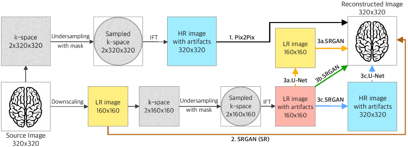
Figure 1: Three possible approaches to downscale and undersample $k$-space. The sampling masks details are given in the supplementary material.

An overview of the different models studied herein is shown in Fig. 1. Using the compressed sensing paradigm [DebatinUltrafastMRIBook, fastmri_challenge, compressed_sens], we aim to accelerate MRI by sampling low resolution or/and partially filled k-space. The partial filling is accomplished by applying patterned masks on the Fourier transform of the original slices. We used the masks proposed by the fastMRI challenge (a central vertical band of $8\%$ of the value is fixed and the remaining bands are sampled randomly), as well as the radial and the spiral sampling trajectories that are popular in the field of compressed sampling [sampling_traj]. The three types of masks considered and the effect of them on the images are shown in the supplementary material.

We used Pix2Pix [pix2pix] as an image-to-image translation method to correct the artifacts introduced by the k-space undersampling and SRGAN [srgan] to upscale the low-resolution images to their original size of $320\times 320$. Interested in preserving the high-frequency components, we used the MSE of the feature maps obtained with the VGG16 pre-trained on ImageNet 31^th layer for the perceptual loss, relying on the reports that convolutional networks pre-trained on ImageNet are still relevant for the perceptual losses of MRI images [johnson2016perceptual, percep_loss_mri, synth_ct_mri].

We retrained Pix2Pix and SRGAN (SR, for superresolution alone) entirely on the datasets described above. The combinations of SRGAN and U-Net generators (paths 3a-c in Fig. 1) were trained with SRGAN discriminator and a joint back-propagation. We also considered SRGAN for the direct reconstruction without the U-Net (path 2 in Fig. 1). The quality of the produced images was assessed using the MSE, PSNR and SSIM [ssim] metrics, similarly to SOTA [fastmri_challenge, philips_fastmri].

4 Experiments

We ran extensive series of experiments outlined in Fig. 1. In all SRGAN variants, our models always outperformed bicubic interpolation, which we confirmed for the $\times 2$, $\times 4$, and $\times 8$ upscaling factors. We also observed that Pix2Pix models, following the undersampling with the radial and the spiral masks, always outperformed the fastMRI mask. The difference between the radial and the spiral masks, however, was less pronounced (see Tables 4 and LABEL:sr_results). All experimental results are shown in the format of $\mu\pm\sigma$, where $\mu$ is the average metric value over the test set, and $\sigma$ is its standard deviation.

Acc. /	Mask	MSE, $\times 10^{-4}$	PSNR	SSIM, $\times 10^{2}$
frac. of
k-space
$\times 2$ 50%	fastMRI	14.39 $\pm$ 3.33	28.53 $\pm$ 0.96	94.02 $\pm$ 3.19
	spiral	6.14 $\pm$ 2.13	32.37 $\pm$ 1.47	96.84 $\pm$ 2.22
	radial	5.08 $\pm$ 1.83	33.20 $\pm$ 1.47	97.70 $\pm$ 1.74
$\times 4$ 25%	fastMRI	27.93 $\pm$ 6.07	25.64 $\pm$ 0.93	90.65 $\pm$ 3.95
	spiral	13.96 $\pm$ 3.81	28.70 $\pm$ 1.15	93.56 $\pm$ 3.52
	radial	11.81 $\pm$ 4.62	29.51 $\pm$ 1.37	94.46 $\pm$ 3.93
$\times 8$ 12.5%	fastMRI	54.41 $\pm$ 12.13	22.75 $\pm$ 0.98	85.74 $\pm$ 4.21
	spiral	28.00 $\pm$ 7.67	25.68 $\pm$ 1.13	89.45 $\pm$ 4.38
	radial	21.12 $\pm$ 5.45	26.89 $\pm$ 1.08	91.23 $\pm$ 4.61
$\times 16$ 6.25%	spiral	45.04 $\pm$ 9.89	23.57 $\pm$ 1.00	85.93 $\pm$ 3.90
	radial	42.21 $\pm$ 9.78	23.87 $\pm$ 1.07	87.12 $\pm$ 4.53
$\times 32$ 3.125%	spiral	69.00 $\pm$ 17.48	21.76 $\pm$ 1.17	82.37 $\pm$ 4.84
	radial	65.62 $\pm$ 19.70	22.02 $\pm$ 1.31	83.06 $\pm$ 5.76

Table 1: Pix2Pix model results.

The Structural Similarity Index Measure (SSIM) is defined by: SSIM(x, y)=(2 μxμy+c1)(2 σx y+c2)(μx2+μy2+c1)(σx2+σy2+c2), where $\mu_{x}$ is the average of $x$; $\mu_{y}$ is the average of $y$; $\sigma_{x}^{2}$ is the variance of $x$; $\sigma_{y}^{2}$ is the variance of $y$; $\sigma_{xy}^{2}$ is the covariance of $x$, $y$; $c_{1}=\left(k_{1}L\right)^{2},c_{2}=\left(k_{2}L\right)^{2}$ are constants used for computational stabiltiy; $L$ is the total intensity range; we set $k_{1}=0.01$ and $k_{2}=0.03$, as indicated in [ssim].

E. Combined models with extreme acceleration factors

We present here the detailed results obtained with our different models at all acceleration factors.

Mask	Model	MSE, $\times 10^{-4}$	PSNR	SSIM, $\times 10^{2}$
fastmri	SRGAN	12.98 $\pm$ 3.79	29.04 $\pm$ 1.22	94.84 $\pm$ 2.55
	SRGAN+U-Net	8.81 $\pm$ 3.08	30.80 $\pm$ 1.44	95.97 $\pm$ 2.17
	U-Net+SRGAN	9.27 $\pm$ 3.28	30.56 $\pm$ 1.41	95.69 $\pm$ 2.69
spiral	SRGAN	7.66 $\pm$ 2.94	31.47 $\pm$ 1.66	96.28 $\pm$ 2.26
	SRGAN+U-Net	7.02 $\pm$ 2.84	31.88 $\pm$ 1.73	96.51 $\pm$ 2.06
	U-Net+SRGAN	7.09 $\pm$ 2.82	31.81 $\pm$ 1.65	96.39 $\pm$ 2.37
radial	SRGAN	6.25 $\pm$ 2.63	32.40 $\pm$ 1.78	96.95 $\pm$ 1.95
	SRGAN+U-Net	6.05 $\pm$ 2.64	32.58 $\pm$ 1.87	97.01 $\pm$ 1.87
	U-Net+SRGAN	6.13 $\pm$ 2.62	32.48 $\pm$ 1.75	96.92 $\pm$ 2.11

Table 5: Low-Resolution ($160\times 160$) model with $\times 2$ undersampling, total acceleration: $\times 8$, fraction of k-space: $12.5\%$.

Mask	Model	MSE, $\times 10^{-4}$	PSNR	SSIM, $\times 10^{2}$
fastmri	SRGAN	23.07 $\pm$ 6.30	26.53 $\pm$ 1.17	92.40 $\pm$ 2.93
	SRGAN+U-Net	15.97 $\pm$ 4.77	28.15 $\pm$ 1.26	94.00 $\pm$ 2.61
	U-Net+SRGAN	18.55 $\pm$ 5.88	27.51 $\pm$ 1.28	93.32 $\pm$ 3.27
spiral	SRGAN	17.29 $\pm$ 5.05	27.79 $\pm$ 1.20	93.32 $\pm$ 2.88
	SRGAN+U-Net	13.61 $\pm$ 4.11	28.85 $\pm$ 1.26	94.19 $\pm$ 2.58
	U-Net+SRGAN	13.49 $\pm$ 4.18	28.89 $\pm$ 1.27	94.08 $\pm$ 3.39
radial	SRGAN	12.71 $\pm$ 4.07	29.18 $\pm$ 1.38	94.54 $\pm$ 2.79
	SRGAN+U-Net	11.44 $\pm$ 3.90	29.66 $\pm$ 1.46	94.92 $\pm$ 2.59
	U-Net+SRGAN	11.39 $\pm$ 3.92	29.67 $\pm$ 1.42	94.79 $\pm$ 3.23

Table 6: Low-Resolution ($160\times 160$) model with $\times 4$ undersampling, total acceleration: $\times 16$, fraction of k-space: $6.25\%$.

Mask	Model	MSE, $\times 10^{-4}$	PSNR	SSIM, $\times 10^{2}$
fastmri	SRGAN	49.63 $\pm$ 13.10	23.19 $\pm$ 1.14	87.19 $\pm$ 3.49
	SRGAN+U-Net	36.99 $\pm$ 9.93	24.47 $\pm$ 1.16	89.57 $\pm$ 3.10
	U-Net+SRGAN	38.72 $\pm$ 11.65	24.30 $\pm$ 1.26	89.09 $\pm$ 3.82
spiral	SRGAN	30.89 $\pm$ 7.43	25.23 $\pm$ 1.04	89.86 $\pm$ 3.33
	SRGAN+U-Net	23.65 $\pm$ 6.13	26.40 $\pm$ 1.11	91.43 $\pm$ 2.96
	U-Net+SRGAN	24.48 $\pm$ 6.76	26.27 $\pm$ 1.17	91.16 $\pm$ 3.68
radial	SRGAN	25.29 $\pm$ 6.90	26.13 $\pm$ 1.16	91.34 $\pm$ 3.16
	SRGAN+U-Net	20.70 $\pm$ 5.91	27.01 $\pm$ 1.21	92.40 $\pm$ 2.96
	U-Net+SRGAN	20.88 $\pm$ 6.09	26.98 $\pm$ 1.22	92.13 $\pm$ 3.62

Table 7: Low-Resolution ($160\times 160$) model with $\times 2$ undersampling, total acceleration: $\times 32$, fraction of k-space: $3.125\%$.

Mask Model MSE, $\times 10^{-4}$ PSNR SSIM, $\times 10^{2}$ spiral SRGAN 46.46 $\pm$ 10.66 23.44 $\pm$ 1.01 86.80 $\pm$ 3.29 SRGAN+U-Net 38.09 $\pm$ 9.34 24.32 $\pm$ 1.09 88.42 $\pm$ 3.16 U-Net+SRGAN 38.76 $\pm$ 10.41 24.27 $\pm$ 1.16 88.32 $\pm$ 3.78 radial SRGAN 42.97 $\pm$ 10.13 23.79 $\pm$ 1.01 87.71 $\pm$ 3.39 SRGAN+U-Net 35.20 $\pm$ 8.92 24.67 $\pm$ 1.08 89.24 $\pm$ 3.19 U-Net+SRGAN 35.64 $\pm$ 9.38 24.63 $\pm$ 1.13 89.06 $\pm$ 3.73

Table 8: Low-Resolution ($160\times 160$) model with $\times 2$ undersampling, total acceleration: $\times 64$, fraction of k-space: $1.5625\%$.

Acc. /	Model	MSE, $\times 10^{-4}$	PSNR	SSIM, $\times 10^{2}$
frac. of
k-space
$\times 4$ 25%	Pix2pix radial	6.98 $\pm$ 2.45	31.80 $\pm$ 1.42	95.97 $\pm$ 3.12
	SRGAN (SR)	3.03 $\pm$ 1.61	35.72 $\pm$ 2.12	98.64 $\pm$ 0.93
$\times 8$ 12.5%	Pix2pix radial	13.98 $\pm$ 4.27	28.72 $\pm$ 1.22	93.41 $\pm$ 3.96
	SRGAN+U-Net radial	6.05 $\pm$ 2.64	32.58 $\pm$ 1.87	97.01 $\pm$ 1.87
$\times 16$ 6.25%	Pix2pix radial	26.14 $\pm$ 7.44	25.99 $\pm$ 1.18	90.55 $\pm$ 4.20
	SRGAN (SR)	11.69 $\pm$ 4.21	29.58 $\pm$ 1.49	95.63 $\pm$ 2.35
	U-Net+SRGAN radial	11.39 $\pm$ 3.92	29.67 $\pm$ 1.42	94.79 $\pm$ 3.23
$\times 32$ 3.125%	Pix2pix radial	54.83 $\pm$ 16.45	22.87 $\pm$ 1.12	86.39 $\pm$ 5.21
	SRGAN+U-Net radial	20.70 $\pm$ 5.91	27.01 $\pm$ 1.21	92.40 $\pm$ 2.96
$\times 64$ 1.5625%	SRGAN (SR)	28.76 $\pm$ 9.67	24.37 $\pm$ 1.13	88.49 $\pm$ 3.32
	SRGAN+U-Net radial	35.20 $\pm$ 8.92	24.67 $\pm$ 1.08	89.24 $\pm$ 3.19

Table 9: Comparison of the best models selected based on the SSIM metric for the brain dataset.

Acc. /	Model	MSE, $\times 10^{-4}$	PSNR	SSIM, $\times 10^{2}$
frac. of
k-space
$\times 4$ 25%	Pix2pix radial	27.95 $\pm$ 19.64	26.23 $\pm$ 2.79	86.69 $\pm$ 5.83
	SRGAN (SR)	8.84 $\pm$ 9.04	32.77 $\pm$ 4.89	94.31 $\pm$ 3.65
$\times 8$ 12.5%	Pix2pix radial	42.26 $\pm$ 29.35	24.54 $\pm$ 2.99	80.97 $\pm$ 8.20
	SRGAN+U-Net radial	21.58 $\pm$ 18.77	27.62 $\pm$ 3.23	88.74 $\pm$ 5.35
$\times 16$ 6.25%	Pix2pix radial	58.09 $\pm$ 40.44	23.22 $\pm$ 3.02	74.87 $\pm$ 10.44
	SRGAN (SR)	26.02 $\pm$ 21.85	27.53 $\pm$ 4.23	85.04 $\pm$ 7.92
	U-Net+SRGAN radial	28.40 $\pm$ 22.85	26.53 $\pm$ 3.31	83.98 $\pm$ 8.42
$\times 32$ 3.125%	Pix2pix radial	77.72 $\pm$ 52.45	21.86 $\pm$ 2.84	70.65 $\pm$ 11.57
	SRGAN+U-Net radial	42.48 $\pm$ 35.12	24.97 $\pm$ 3.56	80.67 $\pm$ 8.90
$\times 64$ 1.5625%	SRGAN (SR)	45.71 $\pm$ 34.51	24.82 $\pm$ 3.88	76.95 $\pm$ 10.65
	SRGAN+U-Net radial	56.72 $\pm$ 41.34	23.44 $\pm$ 3.19	76.24 $\pm$ 10.11

Table 10: Comparison of the best models, selected based on the SSIM metric for the knee dataset.

F. Labeling tool for user study

We used the community version of the open-source labeling tool Label Studio [label-studio] to perform the user study described in the main text, Section 5.We adjusted the user interface to compare the accelerated (left) and the ground truth (right) images based on tree IQ criteria on a 4-point scale.

Figure 14: User interface of the tool for the user study. It was used to survey five radiologists about the diagnostic value of the reconstructions.

An example of the user interface is presented in figure 14. Experts were asked to rate the quality of the left (accelerated) image compared to the right one (ground truth). The main element of the interface is the panel section with two images for the radiologists to observe side-by-side. Users can zoom in and zoom out the images using a mouse scroll wheel to conveniently examine the regions of interest. While performing the examination, the users provide their answers to the questions below, using mouse or keyboard shortcuts. Once the evaluation is finished, users press submit button and proceed to another pair of images. Users can also skip a pair of images in case if they face difficulties with scoring a particular case. The examination is finished either when the user decides to stop or when there are no pairs of images left in the test subset.

G. Experimental Setup

Specification of dependencies

All models were implemented using Python 3.8 and PyTorch 1.4. Training models and all the experiments were conducted using Nvidia Tesla V100 with 32 GB RAM.

Adam optimizer is used to train the models, with the initial learning rate being equal to $10^{-4}$. The size of a batch is 4, and the number of epochs is 100. The combined model contains $29.1$M trainable parameters.

Complexity analysis

Training time of the combined models (SRGAN+U-Net, U-Net+SRGAN) are about 60 hours. An average inference time for 100000 slices shown in Table 11.

Training the combined model with the above parameters requires about 11GB of GPU memory. The inference of the combined model requires 2.2GB of GPU memory.

Model	Time, ms	# of Parameters, M
Pix2pix	9.6	26.1
SRGAN(SR) $\times 4$	7.2	5.7
SRGAN(SR) $\times 8$	6.1	5.9
SRGAN(SR) $\times 64$	5.8	6.2
U-Net+SRGAN	10.7	29.1
SRGAN+U-Net	16.9	29.1

Table 11: An average inference time of the models per slice in milliseconds and the number of trainable parameters.