The Anatomy of an Unusual Edge-on Protoplanetary Disk. II.
Gas temperature and a warm outer region

Abstract

We present high-resolution ¹²CO and ¹³CO 2–1 ALMA observations, as well as optical and near-infrared spectroscopy, of the highly-inclined protoplanetary disk around SSTC2D J163131.2-242627. The spectral type we derive for the source is consistent with a $\rm 1.2\,M_{\odot}$ star inferred from the ALMA observations. Despite its massive circumstellar disk, we find little to no evidence for ongoing accretion on the star. The CO maps reveal a disk that is unusually compact along the vertical direction, consistent with its appearance in scattered light images. The gas disk extends about twice as far away as both the submillimeter continuum and the optical scattered light. CO is detected from two surface layers separated by a midplane region in which CO emission is suppressed, as expected from freeze-out in the cold midplane. We apply a modified version of the Topographically Reconstructed Distribution method presented by Dutrey et al. (2017) to derive the temperature structure of the disk. We find a temperature in the CO-emitting layers and the midplane of $\sim$33 K and $\sim$20 K at $\rm R<200$ au, respectively. Outside of $\rm R>200$ au, the disk’s midplane temperature increases to $\sim$30 K, with a nearly vertically isothermal profile. The transition in CO temperature coincides with a dramatic reduction in the sub-micron and sub-millimeter emission from the disk. We interpret this as interstellar UV radiation providing an additional source of heating to the outer part of the disk.

1 Introduction

Protoplanetary disks are the birth site of planetary systems, and their structure can provide key insights on the planet formation process itself (Andrews, 2020, and references therein). The radial structure of protoplanetary disks has been thoroughly studied in both gas and dust components thanks in large part to ALMA (e.g., Andrews et al., 2018). These observations have revealed the prevalent occurrence of small scale structures such as rings and spiral arms, which have been associated with planets and other physical mechanisms acting in the disks (Dong et al., 2016; Christiaens et al., 2014; Pinte et al., 2019; Zhang et al., 2015; Gonzalez et al., 2017). For disks that have been mapped in both continuum and line emission, it has been revealed that the submillimeter-emitting dust component is much less extended radially than the gas component (Mannings & Sargent, 1997; Ansdell et al., 2018; Boyden & Eisner, 2020). This is generally interpreted as the result of radial drift induced by the drag forces that the gas induces on large dust grains (e.g., Birnstiel & Andrews, 2014; Cleeves et al., 2016), although differences in integrated optical depth could also be at play (Facchini et al., 2017). To fully characterize a protoplanetary disk, it is therefore important to use multiple tracers. In addition to submillimeter continuum and line emission maps, scattered light can be used to trace micron-sized grains, which are expected to be well coupled to the gas (e.g., Barrière-Fouchet et al., 2005) but whose surface brightness is independent of the local temperature.

The vertical structure of protoplanetary disks, on the other hand, has not been studied in as much detail due to a combination of optical depth and projection effects. Disks are expected to be in vertical hydrostatic equilibrium, whereby the vertical component of stellar gravity is balanced by the thermal pressure of the gas. Scattered light images confirm that small dust is lifted up to a flared upper surface, (e.g., Avenhaus et al., 2018) but the height of this $\tau=1$ surface above the midplane can be any number of scale heights depending on the local surface density. While the mass of the central star, which determines the first force, can be derived kinematically from the gas’ orbital motion (e.g., Huélamo et al., 2015; Simon et al., 2019), the pressure gradient is set by the vertical density and temperature profiles in the disk, which is not as readily accessible to observations. Interestingly, recent studies have provided model-independent methods to tomographically determine the gas temperature structure of protoplanetary disks (Dutrey et al., 2017; Pinte et al., 2018; Dullemond et al., 2020; Teague et al., 2020). These methods are applicable to spatially and kinematically resolved disks where the gas component is sufficiently optically thick so that the gas intensity can be transformed into brightness temperature via the Plank equation. These methods open new avenues to address questions related to vertical snow lines (Pinte et al., 2018), the extent of gas depletion in frozen-out regions (Dullemond et al., 2020), and the role of external sources of irradiation such as the interstellar radiation field (Dutrey et al., 2017).

While these temperature retrieval methods can be used for disks at moderate inclination (Pinte et al., 2018; Dullemond et al., 2020), the spatial confusion introduced by projection effects can only be alleviated by kinematics under favorable circumstances. Disks at high inclinations ($i\gtrsim 75$°), often dubbed edge-on disks, offer a distinct advantage by preventing the two disk surfaces to be projected on top of one another, making the tomographic temperature reconstruction much easier (Dutrey et al., 2017). Our team has designed a method to identify new edge-on protoplanetary disks using Spitzer mapping of star-forming regions and obtaining confirmation images with HST, identifying a dozen new such systems to complement the existing sample (Stapelfeldt et al., 2014).

In this study, we focus on SSTC2D J163131.2-242627, hereafter Oph163131, a member of the Ophiuchus star-forming region (Evans et al., 2009; Hsieh & Lai, 2013) located at a distance of $d=147\pm 3$ pc (Ortiz-León et al., 2017). The central source of Oph163131 does not have a published spectrum, and therefore the stellar parameters of this source were highly uncertain prior to this study. The disk surrounding Oph163131 was unambiguously revealed to be edge-on with a radius of about 190 au in HST imaging (Stapelfeldt et al., 2014), as well as in subsequent ALMA continuum survey observations (Cox et al., 2017; Cieza et al., 2019). We have obtained dedicated high-resolution ALMA observations, which are presented in Villenave et al. (2020). In a companion paper (Wolff et al., in prep., hereafter Paper I), we simultaneously modeled the HST scattered light image and the ALMA continuum map. The latter is vertically much thinner, and the radiative transfer model demonstrates that the disk has undergone significant settling.

In this paper, we present and analyze new ALMA CO observations of the Oph13131 disk, as well as the first optical and infrared spectra of this star. In particular, we develop a slightly modified version of the Tomographically Reconstructed Distribution (TRD) method (Dutrey et al., 2017) to account for non-perfectly edge-on disk, and we apply it to the disk around Oph163131 in both ¹²CO J = 2 – 1 and ¹³CO J = 2 – 1 isotopologues. Interferometric and spectroscopic observations of Oph163131 are presented in Section 2. Observational results such as spectral typing of the central source and dynamical mass estimates are presented in Section 3. In Section 4, we describe the method used to reconstruct the temperature structure of Oph163131 and present its temperature distribution. In Section 5, we put Oph163131 in context by comparing it with other disk sources with independently measured temperature profiles. We contrast the inner disk region’s temperature against models that reproduce the ALMA dust continuum and scattered light images. In addition, we present models that include photodissociation, photodesorption, and enhanced UV irradiation as possible mechanisms to explain the observations. In Section 6, we present our conclusions.

2 Observations and data reduction

2.1 ALMA Continuum and CO Maps

We observed Oph163131 with ALMA in Band 6 as part of project 2016.1.00771.S (PI: Duchêne). The spectral set-up was divided into two 1.9 GHz continuum spectral windows, of rest frequency 216.5 GHz and 219.6 GHz, and three spectral windows that were set-up to include the ¹²CO, ¹³CO, and C¹⁸O J = 2 - 1 transitions at 230.538 GHz, 220.399 GHz and 219.56 GHz, respectively. The line spectral windows have native velocity resolutions of 0.16 km s^-1 for ¹³CO, and C¹⁸O and 0.085 km s^-1 for ¹²CO. The source was observed using two different array configurations, specifically a compact and an extended configuration on April 25, 2017 and on July 7, 2017, respectively. The baselines ranged from 15 m to 2650 m between the two configurations, and the total observing time on source was 40 minutes. The raw data were calibrated using the CASA pipeline version 4.7.2.

To maximize the dynamical range, we performed phase self-calibration from the continuum data from both configurations. We extracted the continuum images using the CASA tclean task on the combined data, with a Briggs parameter of 0.5. The resulting beam size is 0$\farcs$23$\times$0$\farcs$13. The continuum image is further analyzed in Paper I. After applying the continuum self-calibration solutions to all spectral windows, we extracted the emission lines from the calibrated visibilities by subtracting continuum emission using the uvcontsub function in CASA. In addition to the continuum subtracted data, we produced a non-continuum subtracted dataset to test whether our modeling method is affected by possible over-subtraction of the continuum in optically thick regions of the disk. We binned the native spectral resolution to 0.25 km s^-1 and used Briggs parameter of 0.5 to create higher signal-to-noise (S/N) line images. The resulting beam were 0$\farcs$25$\times$0$\farcs$20 for ¹²CO and 0$\farcs$26$\times$0$\farcs$20 for ¹³CO, and C¹⁸O. The S/N of the C¹⁸O isotopologue was not high enough to produce a dataset we can analyze.

2.2 JCMT CO map

On April 16, 2011, we obtained ¹²CO J = 3 - 2 data from the Heterodyne Array Receiver Program (HARP) at the 15-m James Clerk Maxwell Telescope (JCMT). An 8′$\times$8′  map around Oph 163131 was acquired at a rest frequency of 345 GHz using 8192 ACSIS channels with a bandwidth coverage of 250 MHz at a spectral resolution of 30 kHz (0.025 $\rm km\,s^{-1}$). The observations were performed in good weather conditions with measured zenith opacities at 225 GHz ($\uptau_{\rm 225GHz}$) varying from 0.09 to 0.1.

The HARP data was reduced using the SMURF code and a data cube was created with the MAKECUBE task. The pixel size of the data cube was set to 6″  which oversamples the 14″  JCMT main beam size (at 345 GHz). In order to increase the S/N of the data, the native velocity resolution was binned to 0.25 $\rm km\,s^{-1}$. At this velocity resolution the measured antenna temperature noise is $\rm\sigma_{TA*}=0.3\,K$ per 0.25 $\rm km\,s^{-1}$, or equivalently $\rm\sigma_{Jy}=9\,Jy$ per 0.25 $\rm km\,s^{-1}$. This conversion was performed using $\rm S(Jy)=15.6\,T_{A}(K)^{*}/\eta_{a}$, where $\eta_{a}=0.52$ is the aperture efficiency of HARP.

2.3 SOAR Optical Spectroscopy

We obtained an optical spectrum of Oph163131 on May 19, 2013, with the Goodman spectrograph installed on the SOAR 4.1m telescope at Cerro Tololo. Two 900 second spectra were acquired while dithering along the 0$\farcs$46 slit. The object was observed at an airmass of 1.01. We used the 400 lines/mm grating and the red camera, which yields a spectral resolution of $\sim$1850 over the full 3400–7500 Å  wavelength range. Spectral images were reduced using the IRAF ccdproc package. A narrow feature in the quartz flat field lamp was removed using procedures within the IRAF twodspec package, as customized by SOAR observatory staff (“Removing arc from GOODMAN 600b flatfield”, T. Ribeiro, private communication). Spectral extraction and wavelength calibration referencing SOAR mercury/argon arcs were performed using IRAF doslit procedures.

2.4 IRTF Near-infrared Spectroscopy

Our near-infrared (NIR) observations of Oph163131 were carried out with the 3.0 m NASA Infrared Telescope Facility (IRTF) on Maunakea, Hawaii on 2019 May 16. We used the upgraded SpeX instrument in the short crossdispersed (SXD) mode, which covers the 0.7 $\micron$ to 2.5 $\micron$ region in each exposure (Rayner et al., 2003), and the 0$\farcs$5 wide slit, which gives a resolving power of $\rm R=1\,200$. Our target was nodded along the slit, with two exposures taken at each nod position. The total exposure time was driven by our goal to get a spectrum with signal-to-noise ratio S/N $>30$ in the H-band. The individual exposure times were limited to three minutes to ensure that the telluric emission lines would cancel when consecutive images taken at alternate nod positions were subtracted. After observing Oph163131, we acquired an A0 telluric standard star within 0.1 air masses for telluric correction purposes.

A thorium-argon lamp was observed for wavelength calibration, and a quartz lamp spectrum was acquired for flat fielding. The SpeX data were flat-fielded, extracted, and wavelength-calibrated using Spextool (Cushing et al., 2004). After extraction and wavelength calibration, the individual extracted spectra were co-added using xcombspec. Xtellcor was then used to construct a telluric correction model using the observed A0 standard, after which the observed spectrum of the target was divided by the telluric model. Finally, xmergeorders was used to combine the spectra in the separate orders into one continuous spectrum.

Although the SXD mode of SpeX provides a wavelength coverage down to 0.7 $\micron$, the low S/N at wavelengths shortward of about 1 $\micron$ precludes connecting the NIR spectrum of Oph163131 with its optical counterpart.

3 Observational Results

3.1 Spectral Characterization

To the best of our knowledge, the optical and near-infrared spectra of Oph 163131 presented here are the first of this source. In edge-on disks, the smooth scattering properties of astronomical dust preserve the spectral features associated with the central source (Appenzeller et al., 2005). Therefore, we use our SOAR and SpeX spectra to 1) estimate the spectral type, hence the physical properties of the central star, and 2) evaluate the accretion status of the system based on the strength of its emission lines.

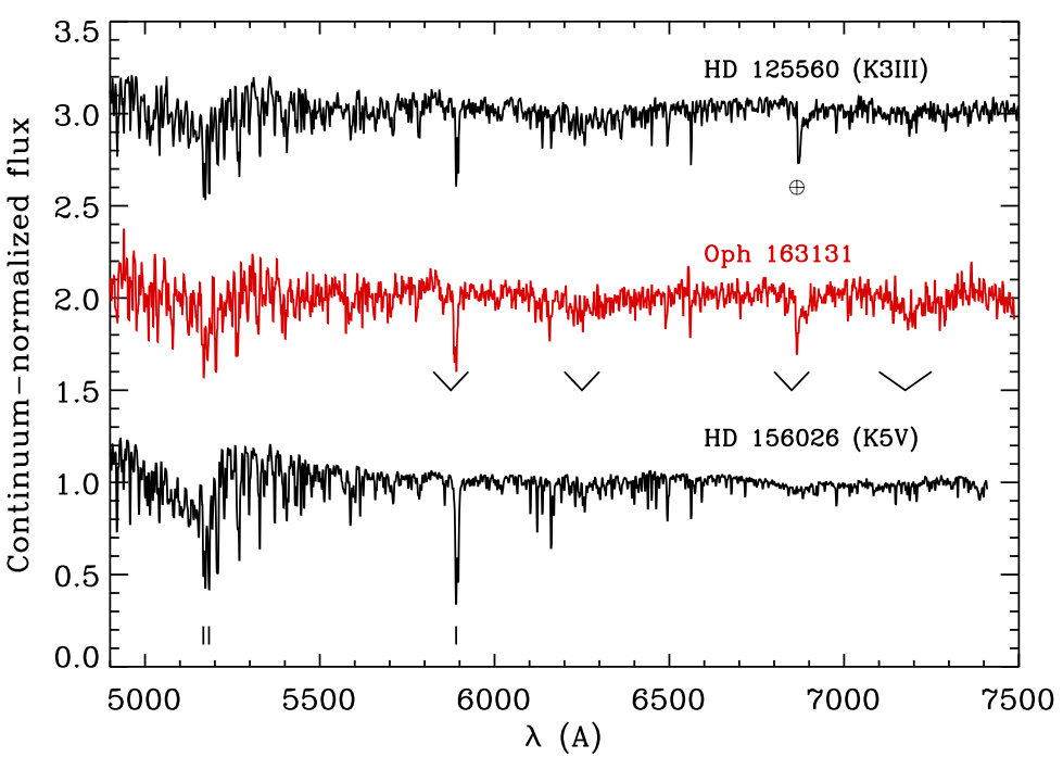
Figure 1: Spectrum of Oph 163131 in the optical (top left panel) and near-infrared (other panels) compared to dwarfs and giants from the MILES, STELIB and SpeX libraries. In the top left panel, a known telluric feature, weak TiO bandheads, and Mg and Na features are labeled under the top, middle, and bottom spectra, respectively. The spectra are offset vertically for clarity. The optical spectrum is normalized to a low-order polynomial fit to the continuum whereas the near-infrared spectra are spectrophotometrically calibrated.

In the absence of spectrophotometric calibration and since scattering off the disk can alter the apparent colors of the central source for our optical spectrum, we focus our spectral analysis on narrow spectral features rather than on the global shape of the continuum. After extracting the 4700–7500 Å spectral range, where the signal-to-noise is sufficient, we fit the spectrum with a polynomial of order 6 and divide it by spectrum. Polynomial orders lower than 4 or higher than 7 leave small unwanted residuals, which do not strongly impact the stellar classification but look artificial in the stellar spectrum. The resulting continuum-normalized spectrum is shown in the top-left panel of Figure 1. The most prominent feature in the spectrum is the sharp Na I D absorption line at 5890 Å and the complex of lines surrounding the 5150 Å Mg line. The main TiO bands (at around 5900, 6200, 6800, and 7100 Å), which are typically seen in K5 and later type stars, are weak in the spectrum of Oph 163131. The combination of these observations suggests that, in the optical, Oph163131 is an early- to mid-K spectral type source (Jacoby et al., 1984; Allen & Strom, 1995). In the near-infrared, the spectrum of Oph 163131 (also shown in Figure 1) shows a number of atomic features across the $J$, $H$ and $K$ band, as well as modest CO bandheads beyond 2.29 $\mu$m. The relative strengths of these features, when compared to the spectral library of Rayner et al. (2009), as well as the overall shape of the continuum, are consistent with a mid to late-K type star.

We further this analysis by comparing the spectrum of Oph 163131 to that of templates from the MILES and STELIB (in the optical, Sánchez-Blázquez et al., 2006; Falcón-Barroso et al., 2011; Le Borgne et al., 2003) and IRTF/SpeX (in the near-infrared Rayner et al., 2009) libraries. We perform the comparison with both dwarfs and giants. To circumvent issues such as stellar rotation and line veiling induced by accretion, we limit our analysis to a visual inspection that focuses equally on the strength of individual absorption features and on small-scale continuum structure related to molecular bands. This is sufficient for the level of precision needed for our analysis. The closest match for the optical spectrum of Oph 163131 is a K3–K4 giant, while in the infrared the spectrum resembles a K4–K5 dwarf. Such discrepant spectral type measurement at different wavelengths could be simply due to the visual characterization of the stellar spectra. However, it might also be a real phenomenon, as spectroscopic studies at high-resolution have shown that starspots on the surfaces of young stars produce an observed temperature dependency with wavelength (see e.g., Flores et al., 2020; Sokal et al., 2018). The stellar luminosity (and hence the luminosity classification) of Oph163131 is uncertain because of dilution by an unknown amount through scattering off the disk. Therefore, it cannot be calculated using the distance to the star and photometry. In any case, since our best match luminosity type lay between dwarfs (V) and giants (III), we adopted a sub-giant (IV) luminosity classification for Oph 163131. This is consistent with previous work where sub-giant surface gravities have been measured for young stars (Doppmann et al., 2005; Flores et al., 2019). In summary, and considering the optical and IR spectra of the star, we classify Oph163131 as a K4 IV star, with a spectral type uncertainty of about one subtype. This implies a stellar mass of $\sim 1\,\rm M_{\odot}$ based on recent dynamical mass measurements for stars in Taurus and Ophiuchus (Simon et al., 2019) and also from stellar evolutionary models (e.g., Feiden, 2016; Somers & Pinsonneault, 2015).

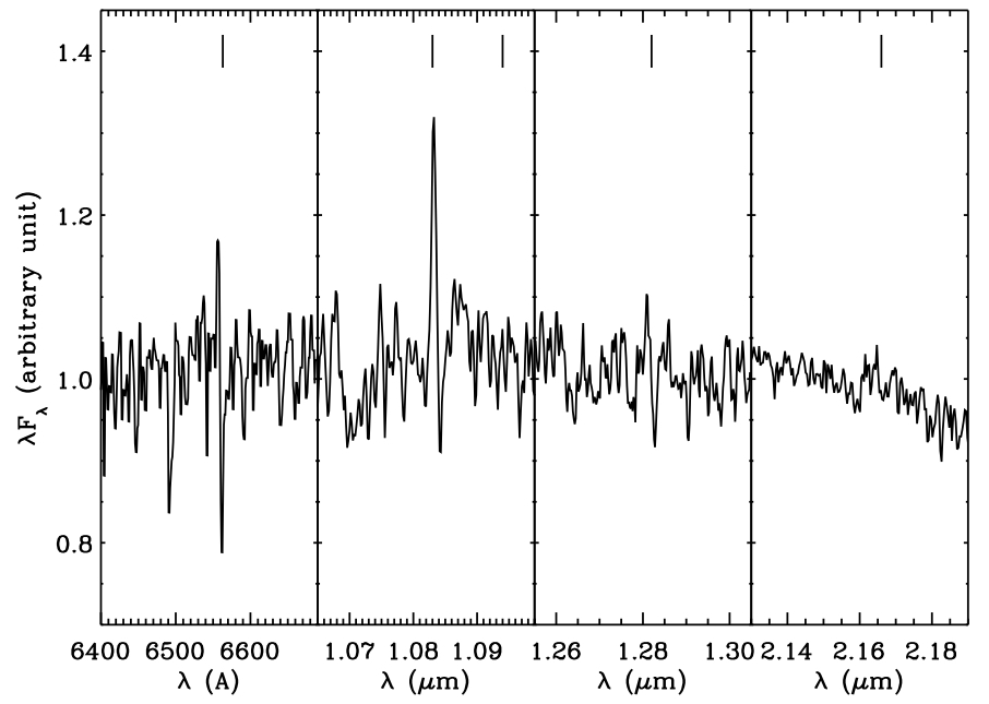
Figure 2: Main emission lines in the spectrum of Oph 163131. From left to right, the lines are H$\alpha$, He I 1.08 $\mu$m and H Pa $\gamma$, H Pa $\beta$ and H Br $\gamma$. The wavelength of each feature is indicated by a vertical bar above the spectrum.

The optical spectrum of Oph 163131 stands out from that of other edge-on disks systems for the absence of strong emission lines (e.g., Appenzeller et al., 2005). Indeed, we only detect a very weak H$\alpha$ emission component, with an equivalent width of 0.6$\pm$0.1 Å, superimposed on a significant photospheric absorption feature. Such a weak H$\alpha$ line, especially in the absence of other accretion- or outflow-related emission lines, generally indicates that the central source is currently not accreting at an appreciable level (e.g., Barrado y Navascués & Martín, 2003; Duchêne et al., 2017), i.e., Oph163131 can be classified as a Weak-line T Tauri star. This assessment is confirmed at first glance by our near-infrared spectrum, in which no significant Pa $\gamma$, Pa $\beta$ or Br $\gamma$ emission is detected (see Fig. 2), although it is worth pointing out that these lines are less sensitive to low levels of accretion onto T Tauri stars (e.g. Folha & Emerson, 2001; Alcalá et al., 2014).

The only other significant emission line detected in our spectra is the 1.08 $\mu$m He I line, with an equivalent width of 2.0$\pm$0.2 Å. This line has a complex origin, with possible contributions from chromospheric activity, disk and/or stellar wind, and accretion onto the central star (Edwards et al., 2006). Surprisingly, all T Tauri stars with an He I emission line as strong as Oph163131 are accretors (see Fig. 3), leading to an apparent paradox. The ultimate diagnostic of the origin of the He I line lies in the line profile, (Fischer et al., 2008; Thanathibodee et al., 2018), which our low-resolution data do not allow us to analyze. We are therefore left with an ambiguous classification for Oph163131. We note that the edge-on nature of the object could lead to biased estimates of line equivalent width if the emission is spatially distinct from the star itself. However, if the emission is chromospheric in nature, its origin is at the stellar surface, and thus our equivalent width estimates would be unbiased.

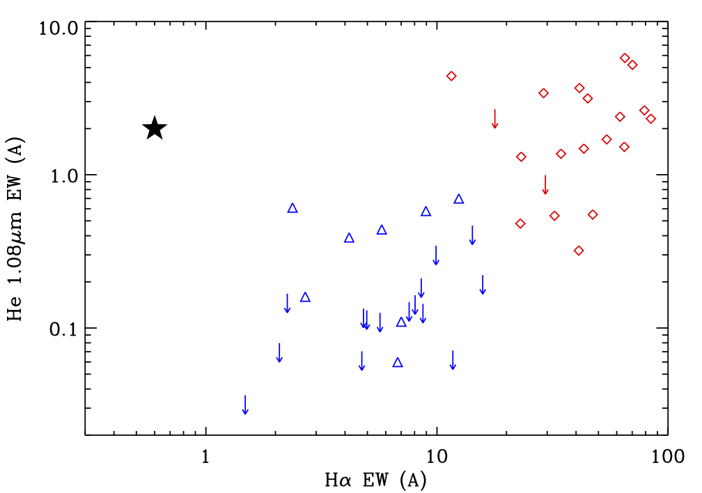
Figure 3: Comparison between the equivalent width of the H$\alpha$ and He I 1.08 $\mu$m lines among accreting (red diamonds) and non-accreting (blue triangles) T Tauri stars. Data are from Edwards et al. (2006), Manara et al. (2013) and Alcalá et al. (2014). Arrows mark upper limits on the He I line. The black star indicates results for Oph163131.

In summary, while Oph163131 is unlikely to be accreting at a high rate, existing data are consistent with both 1) an object with a modest amount of accretion (and a remarkably weak H$\alpha$ line), and 2) a non-accreting, chromosphere-dominated emission line spectrum (albeit with an unusually strong He I 1.08 $\mu$m line). Only higher spectral resolution observations can solve this ambiguity.

3.2 Dynamical Mass Measurement

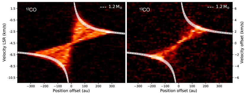
Figure 4: Position-velocity diagrams along the major axis of Oph163131. The ¹²CO(2–1) isotopologue is shown on the left panel with the LSR velocity of the system in left y-axis. The ¹³CO(2–1) is shown on the right panel using the velocity offset coordinates and assuming a systemic velocity of $v_{sys}=-4.4\rm\,km\,s^{-1}$. The white dashed lines correspond to a Keplerian velocity profile for a star of 1.2 $\rm M_{\odot}$. The white filled region is bracketed by upper and lower limits of 1.4 $\rm M_{\odot}$ and 1.0 $\rm M_{\odot}$, respectively.

In the previous section, we used the spectral type derived for Oph163131 and results from stellar evolutionary models to infer the mass of the star. However, it is possible to directly measure the stellar mass using the disk’s CO data and the ‘position-velocity (PV) diagram’ technique (see for example, Huélamo et al., 2015).

In general, dynamical mass measurements using this technique work better when the emission from a disk is optically thin (e.g., ¹³CO or C¹⁸O). This is because optically thin molecules trace the emission closer to the disk’s midplane, or equivalently because there is less confusion with emission arising high up in the disk’s surface. In the case of highly inclined disks $i\gtrapprox 85$°, however, the position of the disk’s major axis approximately coincides with the disk midplane. Therefore low-elevation emission can be observed even for optically thick tracers such as ¹²CO. Since Oph163131 is known to host an almost perfectly edge-on disk, we can confidently calculate the dynamical mass of the star from either of the CO tracers.

The computed PV diagrams in ¹²CO and ¹³CO along the major axis of the disk are shown in Figure 4. In each case, Keplerian velocity profiles of an inclined disk with $i=87\arcdeg$ (the best-fit inclination to the ALMA continuum map from Paper I) with a stellar mass of $\rm 1.2\,M_{\odot}$ were overlaid. The systemic velocity of the disk was estimated to be $v_{sys}=-4.4$ $\rm km\,s^{-1}$, which is further confirmed in Section 3.4 using $\rm{}^{12}CO$ integrated spectrum and channel maps. Although the Keplerian profiles were matched to the data by eye, we are confident in this technique as we have tested it with synthetic disk models computed with MCFOST (Pinte et al., 2006, 2009). We assign conservative upper and lower mass limits to Oph163131 of 1.4 $\rm M_{\odot}$ and 1.0 $\rm M_{\odot}$, respectively. We conclude that the dynamical mass measured for Oph163131 is in agreement with the spectral type derived in Section 3.1.

3.3 Cloud contamination

A crucial part of the temperature reconstruction method explained in Section 4 requires us to determine whether there is emission on a scale much larger than the disk, for example, caused by a molecular cloud at the position of Oph163131. To investigate whether this large scale emission is present or not, we use ¹²CO J = 3–2 single-dish observations acquired with HARP/JCMT (see Section 2.2).

A $\sim$6′$\times$6′  JCMT CO map centered at the position of Oph163131 is shown in Figure 5. Part of the large L1689 molecular cloud is detected East of Oph163131 at velocities ranging from 3.3 to 4.6 $\rm km\,s^{-1}$. The spectrum measured at the location of Oph163131 shows no significant emission above 2$\sigma$ in any of the velocity channels. Conversely, the three spectra measured in different locations of the molecular cloud show prominent emission at $\sim 4\,\rm km\,s^{-1}$. This velocity range does not overlap with the CO emission from the Oph163131 disk in our ALMA data (see Figure 6). Therefore, we conclude from the JCMT data that the cloud emission does not coincide in the spatial or velocity dimensions with that of the disk.

To further investigate whether low levels of cloud emission could affect the disk emission while being undetected in our JCMT data, we consider the ¹²CO and ¹³CO ALMA spectra of Oph163131 (Figure 6). The spectra were computed by summing the flux in a rectangular region of $5.4\arcsec$ along the major axis and $1.5\arcsec$ along the minor axis of the disk. The ¹²CO emission is detected above a $3\sigma$ level between -9.75 and +1.0 $\rm km\,s^{-1}$, while the ¹³CO emission is detected above a $3\sigma$ level in the slightly narrower range from -8.0 to -0.75 $\rm km\,s^{-1}$. This difference is likely due to the lower S/N detection of the latter isotopologue.

Both spectra show the characteristic double peak profile seen in other disks (e.g., Beckwith & Sargent, 1993; Mannings & Sargent, 1997). The nearly perfectly symmetric profile displayed in ¹²CO is a strong indicator that no emission is added or subtracted to the disk. In cases where the line emission from a disk is contaminated by either a background or foreground cloud the observed spectra always display a strongly asymmetric double profile in optically thick tracers such as ¹²CO (see for example, Guilloteau et al., 2016; Perez et al., 2015).

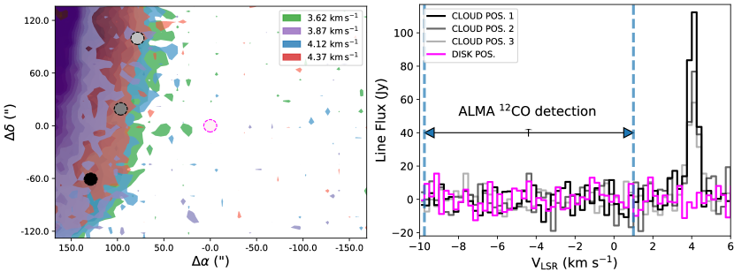
Figure 5: The left panel shows the JCMT ¹²CO J = 3 – 2 intensity map of the large scale structure around Oph163131. In colors we displayed four different velocities channels where the emission of the cloud is the strongest (with $v_{LSR}$ ranging from 3.6 to 4.4 $\rm kms^{-1}$). Four $14\arcsec$-diameter (i.e., beam-sized) circular apertures are overlaid at locations within the cloud (light gray, gray, and black) and at the location of Oph163131 (pink). The right panel shows the JCMT spectra obtained at the locations mentioned above, and using the same colors as the apertures in the left panel. The dashed blue vertical lines and the horizontal arrow depicts the velocity range over which the Oph163131 disk is detected above 3$\sigma$ in the ¹²CO J = 2 – 1 ALMA data. There is no spatial or spectral overlap between the Oph163131 disk and the cloud.

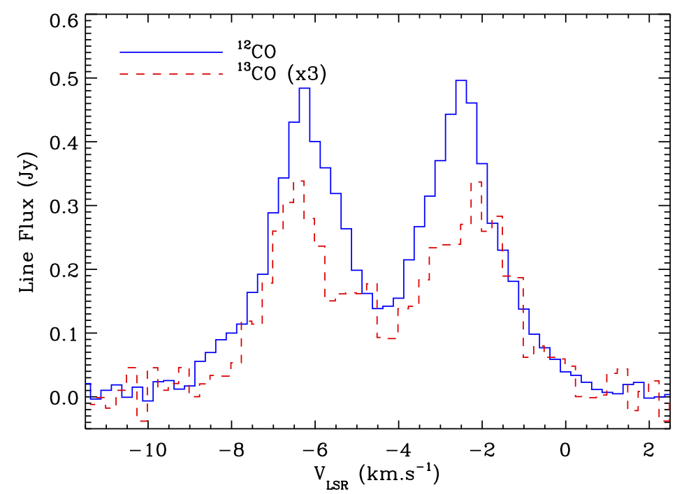
Figure 6: ALMA ¹²CO (in solid blue) and ¹³CO (in dashed red) spectra of the disk around Oph163131. The ¹³CO emission was scaled up by a factor of three for illustrative purposes.

3.4 Disk morphology

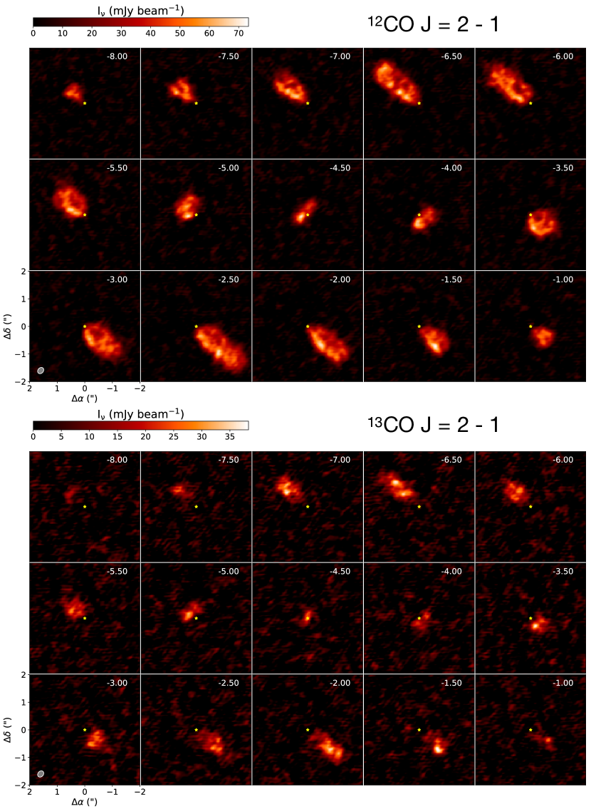
Figure 7: ¹²CO (top) and ¹³CO (bottom) ALMA channel maps of the Oph163131 disk. Each channel shows a square region of $4\arcsec$ in size centered on the predicted stellar position marked with a yellow star. The LSR velocity (in $\rm km\,s^{-1}$) is indicated in the top-right of each channel. The synthesized beam is shown as a grey ellipse in the lower-leftmost channel.

We now describe the morphology of the Oph163131 disk as seen by ALMA. Figure 7 shows the ¹²CO J = 2 - 1 and ¹³CO J = 2 - 1 channel maps of the disk. In both isotopologues, Oph163131 exhibits the typical Keplerian velocity pattern of a highly inclined disk (see for example Dutrey et al., 2017), with ¹²CO having a stronger detection due to the higher peak signal-to-noise ratio of S/N $\sim 24$ per 0.25 $\rm km\,s^{-1}$ compared to the peak signal-to-noise ratio for ¹³CO of only S/N $\sim 12$ per 0.25 $\rm km\,s^{-1}$. Oph163131 is well spatially resolved in both isotopologues with the ¹²CO extending $4.6\arcsec$ along the major axis and $1.2\arcsec$ in the minor axis direction, and ¹³CO extending $3.6\arcsec$ and $0.7\arcsec$ along the major and minor axes, respectively.

In ¹²CO, the disk displays two clear bright layers along the minor axis (in the Southeast and Northwest directions) separated by a darker middle lane. The projected distance between the two bright layers is $\sim 0.45\arcsec$ and the SE layer is $10-20$ mJy brighter than the NW layer. Other ALMA results where CO maps show this type of brightness asymmetry are the Flying Saucer (2MASS J16281370-2431391) (Dutrey et al., 2017) and IM Lup (Pinte et al., 2018). The physical explanation for this phenomenon is the viewing angle of the observer with respect to the disk. Oph163131 is tilted slightly away from a perfectly edge-on configuration, with the SE side being the ‘top’ side as seen from the observer. Geometrical and optical depth effects, in particular the thickness of the CO emitting layer and absorption by the cooler midplane layer, result in the ‘bottom’ layer being partially hidden whereas we can directly see a much larger surface area of the ‘top’ layer. Interestingly, scattered light images of Oph163131 also show the SE layer being brighter than the NW layer, as can be see from Figure 8, where the $\sim 0.6\,\mu\rm m$ HST F606W scattered light image of Oph163131 is overlaid on the ¹²CO integrated intensity (moment zero) map (see also Paper I).

Although the ¹³CO emission is resolved along the minor axis of the disk (over-sampled 2.8 times), it is not possible to distinguish the two emitting layers seen in¹²CO. The combination of a lower S/N and smaller vertical size of the disk in ¹³CO, prevent us from distinguishing any additional structure in this isotopologue.

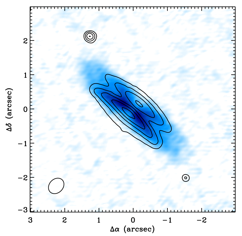
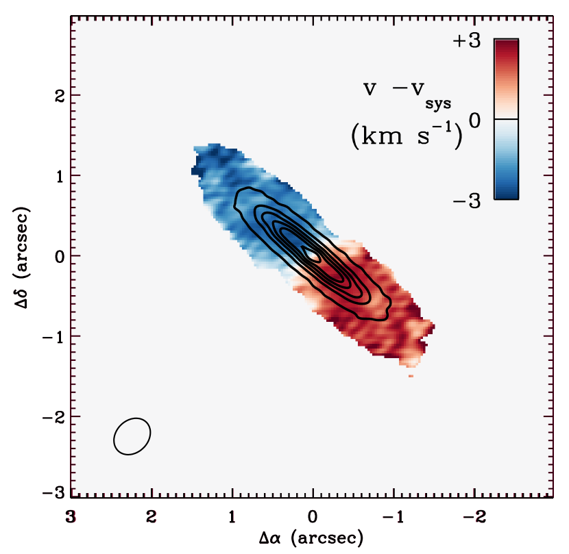
Figure 8: Left panel: Overlay of the ¹²CO zero moment map shown in colors and the HST F606W image described in Paper I in contours of 3, 10, 20, 40 and 60 $\sigma$. The effective ALMA beam is indicated in the bottom left corner whereas two unrelated stars in the HST image are representative of the point spread function in the optical. Right panel: Overlay of the ¹²CO first moment map and the 1.3 mm continuum map described in Paper I. Contours for the continuum map are shown at the 5, 50, 100, 150, 200, 250 and 300$\sigma$ level; the first moment map is only shown where the moment zero exceeds the 5$\sigma$ level.

In Figure 9, we present a comparison between ¹²CO, ¹³CO, and 1.3 mm dust continuum brightness profiles along the minor and major axes of the disk. The left panel of Figure 9 shows that the dust disk is smaller radially by a factor of almost 2 than the ¹²CO gas. Similar results where the gas component extends further in radial direction than the dust component have been reported in the literature and are interpreted as inward radial drift of dust grains (Ansdell et al., 2018). We note that the double peak component in the integrated gas profile is the natural result of the high inclination of the disk, with some self-absorption occurring along the line of sight to the central star. Villenave et al. (2020) measured a full radial extent of $2\farcs 50\pm 0\farcs 01$ for the disk based on the continuum map (see also Paper I). The right panel of Figure 9 demonstrates that the dusty disk is vertically thinner than both gas components, and possibly much thinner as the continuum is unresolved in this direction. From this panel, one can also see an asymmetric profile in the ¹²CO, caused by the brightness differences between the SE and NW layers, but a much more symmetric profile for the ¹³CO component, supporting the fact that no significant structure is detected in ¹³CO.

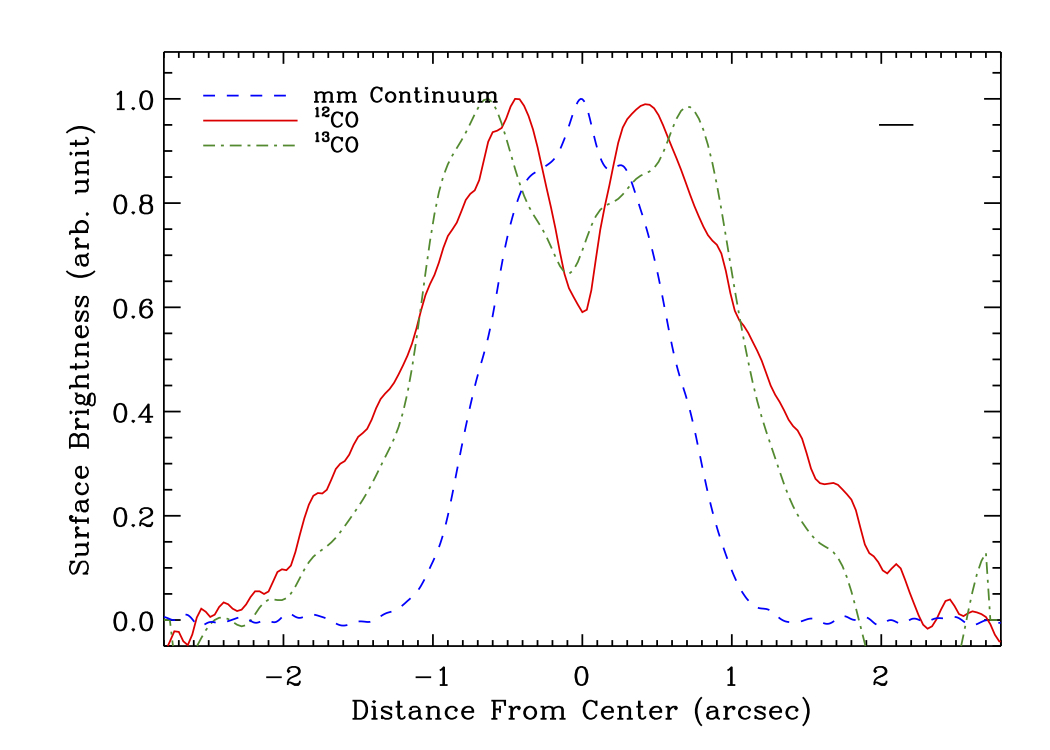
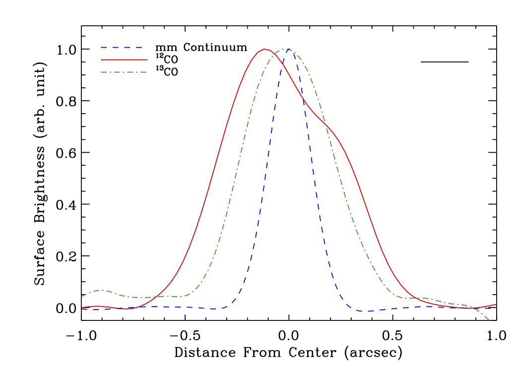
Figure 9: Brightness profiles along the major (left panel) and minor axis (right panel), integrated over the other dimension in both cases, of the dust millimeter continuum, ¹²CO, and ¹³CO data of Oph163131 (dashed blue, solid red and dot-dashed green, respectively). The horizontal ¹³CO profile has been convolved by a Gaussian with a width equal to the minor axis of the beam to improve signal-to-noise. All brightness profiles are displayed in arbitrary units, after normalization to their respective maxima. The horizontal bar in the top right represents the FWHM of the beam along its major axis.

4 Tomographic Gas Temperature Retrieval

4.1 Method

Temperature estimates of protoplanetary disks are often obtained through detailed modeling of (sub)-millimeter observations or from long wavelength coverage SED fitting (e.g., Woitke et al., 2019). In both of these approaches, it is common to parameterize the temperature and the density structure of a disk and then vary many of these parameters until a good match between models and observations is reached. These many parameter fitting techniques are often under-constrained given the real complexity found in high-angular resolution disk observations.

Direct measurement of the temperature structure of disks is therefore not only important in our understanding of the radiative processes of disks, but it can, in principle, also be used to constrain current modeling work. Here we describe a model independent technique developed to measure the temperature structure of protoplanetary disks. This technique, referred to as Tomographically Reconstructed Distribution (TRD) was first implemented by Dutrey et al. (2017) and was applied to the edge-on protoplanetary disk ‘The Flying Saucer’. A similar method was recently implemented by Teague et al. (2020) for Gomez’ Hamburger (2MASS J18091339-3210500).

The TRD technique is a geometrical approach designed to identify parcels of gas on a spatially and spectrally resolved protoplanetary disk and map these parcels of gas onto a 2D radial and vertical structure. This technique assumes that the disk’s inclination angle is close to edge-on and that the disk follows a Keplerian velocity field. Although the latter point is not exactly correct, as gaseous disks are pressure supported systems, and therefore they do not rotate exactly at Keplerian velocities. It has been demonstrated that omitting the pressure term ($-\frac{1}{\rho}\frac{dP}{dr}$) only causes a small over-estimation of the gas velocity at large disk radii. Pinte et al. (2018) analyzed the velocity pattern of the disk around IM Lupi (whose mass is similar to that of Oph163131) and found that the pressure gradient term only increases the rotational velocity of the disk by 0.1 $\rm km\,s^{-1}$ at distances larger than 300 au. Since our disk does not extend beyond 300 au and our velocity resolution is already larger than this effect, we are safe by assuming pure Keplerian rotation.

In order to convert the incident flux emitted from the gaseous component of the disk into brightness temperature, we assume that the gas is in local thermodynamic equilibrium (LTE). The LTE condition is valid in high density regions, for example, towards the midplane of most protoplanetary disks, but not necessarily towards the disk’s photosphere. Besides, when the emission is optically thick and fills the beam, the brightness temperature becomes comparable to the gas’s excitation temperature. This is typically the case for ¹²CO, but it can also be true for the rarer isotopologue ¹³CO (see for example Pinte et al., 2018). Furthermore, the excitation temperature of low-J CO lines, as is our case here, follows very closely the kinematic temperature of the gas (Pavlyuchenkov et al., 2007).

In the following paragraphs, we briefly describe the steps involved in the reconstruction of the temperature distribution of a protoplanetary disk. We refer the reader to Appendix A for the derivation of the equations we used to reconstruct the disk emission.

Our modeling technique depends on the stellar mass ($\rm M_{\ast}$), the distance to the source ($d$), and the inclination angle of the disk relative to the observer ($i$). These values are input into equations (A7) and (A11), which parameterize the radial position ($\rho$), and the altitude above the mid-plane ($z$) of small parcels of gas in a protoplanetary disk as a function of the observed line of sight velocity ($v_{y}$), the impact parameter ($x$), and the projected altitude above the mid-plane ($z^{\prime}$). A PV diagram is then selected at a projected altitude $z^{\prime}$, and the code calculates the radial $\rho$ and altitude $z$ coordinates, in addition to the intensity value $I$ of the disk at such locations. This process is repeated by selecting a new PV cut at a different projected elevation ($z^{\prime}+\Delta z^{\prime}$) to obtain a new set of intensity values for all the radial positions $\rho$ and elevations ($z+\Delta z$). This iteration continues until all the projected altitudes above and below the projected midplane are analyzed.

It is worth noting that in a perfectly edge-on case ($i=90\arcdeg$), the emission obtained from a PV diagram emerges from a fixed elevation in the disk, allowing us to construct a one-to-one mapping between projected and true mid-plane positions. In cases where $i\neq 90\arcdeg$, however, the emission from a PV diagram obtained at a given projected elevation $z^{\prime}$, comes from a range of elevations $\Delta z$ above and below such projected elevation. This is exemplified in Figure 10 where we show the same PV diagram, measured at $z^{\prime}=0$, but we use three different disk inclination angles. In the left panel, where $i=90\arcdeg$, the emission from different radial positions are expected to arise from a unique vertical elevation $z=0$ au. When the inclination is assumed to be $i=87\arcdeg$ (middle panel) the emission from different radial positions emerge from a variety of elevations above the midplane $1\lesssim z\lesssim 10$ au. Lastly, if the inclination is assumed to be $i=84\arcdeg$, then the range of elevations where the emission is assumed to be emitted, is even larger than before $2\lesssim z\lesssim 20$ au. Therefore, we emphasize the importance of considering small deviations out of edge-on inclinations when using the TRD technique.

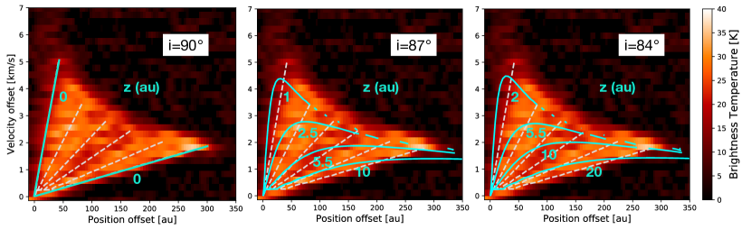
Figure 10: Demonstration of the TRD method assuming three different disk’s inclination angles: $i=90\arcdeg$ (left), $i=87\arcdeg$ (middle), and $i=84\arcdeg$ (right). All three figures show the same PV diagram along the disk’s major axis. White dashed lines correspond to iso-radial lines ranging from 40 to 300 au, these lines remain the same with inclination. Cyan solid lines represent iso-altitude lines (regions at the same vertical distance above the midplane). Assuming a perfectly edge-on disk (left panel) the flux from different radii emerge at a fixed altitude ($z=0$ au in this case). As the disk is declined out of the edge-on position, the observed flux displays a radial and vertical dependency within the PV cut. At an inclination of $i=87\arcdeg$ (middle panel) the emission emerges from altitudes ranging between $1\lesssim z\lesssim 10$ au while at an inclination of $i=84\arcdeg$ (right panel) the emission arises from even higher altitudes, $2\lesssim z\lesssim 20$ au.

After all the intensity values $I$ and spatial coordinates $\rho$ and $z$ from the PV cuts are collected, we construct a two dimensional array of radial (R) and vertical (Z) positions with steps of 10 au in both directions. This spacing size was chosen to oversample by factors of $\sim 3$ and $\sim 4$ the resolution of our observations in the radial and vertical directions, respectively. Intensity values are then assigned to each of these R-Z cells and median values are calculated within each cell. To calculate the statistical uncertainty in our method, we additionally measure the 16th and 84th percentiles of the intensity values for each of the cells, and find a $2-4$ mJy ($1-2$ K temperature) uncertainty in most parts of the disk. Before the median intensity is converted into brightness temperature, each of the R-Z cells with 10 or fewer individual intensity values or cells with median intensity below 9 mJy (or 4.5 K) were masked. This ensures that the statistical computations of the median, the standard deviation, and the percentiles are meaningful. At last, the average intensity values are transformed into brightness temperature using Planck’s equation (1), where T_bg is the microwave background emission of 2.73 K.

$$\rm T_{b}=\frac{h\nu}{k}\left[\ln{\left(\frac{2h\nu^{3}}{I_{\nu}c^{2}}+1\right)}\right]^{-1}+T_{bg}$$ (1)

In Appendix B, we show a variety of tests performed using synthetic disk models computed with MCFOST. These tests, which include disk’s inclination and spatial resolution variations, confirm that the temperature retrieval method works well in the interior regions of the disk where the density is large enough to meet our optical depth criteria.

4.2 The temperature structure of Oph163131

We now apply the TRD method to the ¹²CO J = 2 - 1 and ¹³CO J = 2 - 1 data cubes of Oph163131. We fixed the stellar mass to 1.2 $\rm M_{\odot}$, the disk inclination angle to $i=87\arcdeg$, and the distance to the source to $d=147$ pc. The top panel of Figure 11 shows the result of the reconstructed temperature distribution for the ¹²CO line. The reconstruction technique was applied to both sides of the disk (positive and negative velocities with respect to $v_{sys}$), both of which show a maximum radial extent of $\rm R_{max}=350$ au and altitude above the midplane of $\rm Z_{max}=80$ au. From this plot, we can clearly recognize the ‘top’ and ‘bottom’ layers of the disk, which are separated by a colder midplane that extends from about 100 au to 200 au in radius. The peak brightness temperature on both sides of the disk reaches about the same temperature of $35\pm 2$ K at a distance of 135 $\pm$ 20 au from the center of the disk. The displacement of the peak brightness temperature outside of the inner part of the disk is mostly caused by the beam convolution effects which are described in Appendix B. However, towards the innermost regions of the disk $\rm R\lesssim 1$ au (which cannot be accessed at our spatial resolution) dust absorption could also play a role in decreasing the apparent brightness temperature of the gas and therefore shift the peak temperature position.

In the disk, emission detected at radial distances smaller than $\sim 130$ au are more heavily affected by beam dilution due to the smaller scale height at the inner parts of a flared disk. As demonstrated in Appendix B.3, beam convolution results in underestimating the maximum temperature of the disk and overestimating the gas temperature close to the midplane. The temperature gradient from the ¹²CO reconstructed temperature is therefore only a lower limit to the true temperature gradient in Oph163131.

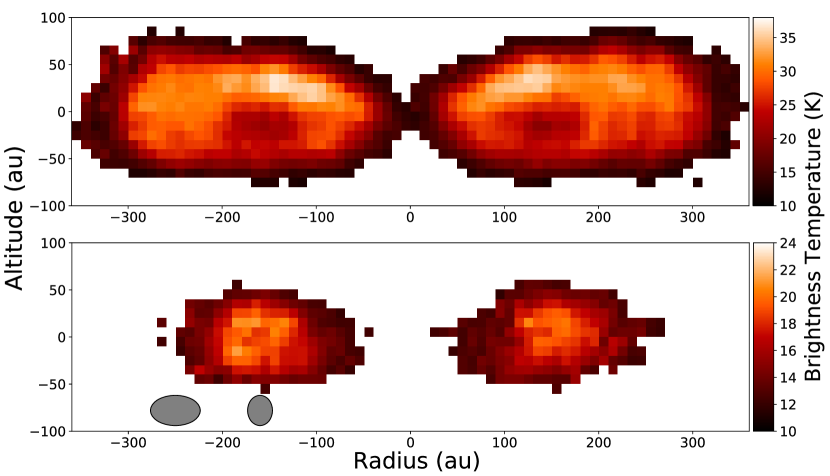
Figure 11: Tomographically reconstructed distribution of the $\rm{}^{12}CO$ (top panel) and the $\rm{}^{13}CO$ (bottom panel) lines. The reconstructed temperature maps are shown in physical units of radius and altitude, both in au. On the $\rm{}^{12}CO$ reconstructed temperature, we distinguish the near and the far emitting layers of the disk. The $\rm{}^{13}CO$ reconstructed temperature, on the other hand, does not show any significant structure. The grey ellipses shown on the top left part of the bottom panel illustrate how the Keplerian velocity shear affect the resolution as a function of radius.

The bottom panel of Figure 11 shows the reconstructed temperature distribution for the ¹³CO isotopologue. This reconstructed distribution is radially and vertically more compact than the ¹²CO temperature distribution, and we only detect emission at vertical distances smaller than 45 au and radial distances between 60 au and 250 au. A similar reduction in the relative height of the CO isotopologue emission layers was identified by Teague et al. (2020) for Gomez’ Hamburger. A combination of lower S/N, lower optical depth, and beam smearing prevent us from identifying clear structures in this isotopologue. The detected ¹³CO emission is unlikely to arise from the midplane due to CO freeze-out; instead, the emission we detect is likely emitted by thin layers just above and below the freeze-out zone, which are completely unresolved by our limited $\sim 0$$\farcs$2 spatial resolution.

On the lower left part of Figure 11, two gray ellipses represent the spatial resolution variations at different radial distances. These radial resolution differences are due to the Keplerian shear velocity of the disk, calculated as $dr=2r\,dv/v(r)$, where $v(r)$ is the Keplerian velocity of the disk and $dv$ is the local line width. For distances smaller than 160 au, the beam size dominates the radial resolution limit of the map, however, at distances larger than 160 au the radial resolution is limited by the Keplerian velocity shear. The two ellipses shown at 160 au and 250 au, represent then radial resolution variations from 30 au and 60 au. We note that the local line width in our dataset is dominated by our velocity resolution of 0.25 $\rm km\,s^{-1}$, and not by the combined thermal and turbulent line broadening, as was the case for the analysis performed on the Flying Saucer (Dutrey et al., 2017).

4.3 Radial and vertical temperature profiles

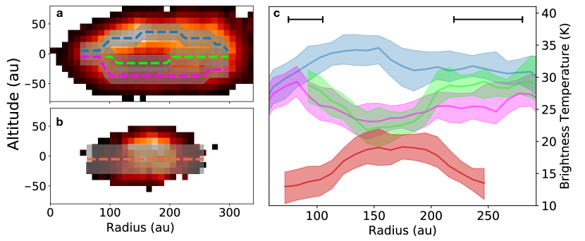
Figure 12: Panels a and b show the left-right averaged temperature distribution from Figure 11. Color lines correspond to a visual trace over the near, far and cold midplane layers for the $\rm{}^{12}CO$, and just center for the $\rm{}^{13}CO$. The wider transparent region next to the white traces correspond to the three pixel (five pixel) vertical average used to create panel c for $\rm{}^{12}CO$ and $\rm{}^{13}CO$, respectively. Panel c shows the traced temperatures as a function of radius for the cold midplane, bottom and top layers of the $\rm{}^{12}CO$ map, and the center temperature for the $\rm{}^{13}CO$ map. The shaded regions around the solid lines, correspond to the temperature uncertainties for each layer. Horizontal bars in panel c, drawn at distances of 100 au and 250 au, depict the changing radial resolution of this method (see subsection 4.2)

To better understand the radial temperature structure of the disk, we show the temperature variation as a function of radius for ¹²CO and ¹³CO in Figure 12. We first averaged both sides (left and right in Figure 11) of the temperatures maps, and then visually identified three distinct layers for the ¹²CO (panel a) and a single layer going through the center of the ¹³CO (panel b). A three pixels average in the vertical direction (24 au) for the ¹²CO, and a five pixels average (40 au) for the ¹³CO were used to compute the temperature profiles shown in panel c.

Panel c of Figure 12, shows that the temperature of the top layer (in blue) increases from $27$ K at 60 au to a peak temperature of $35$ K at 150 au, then it declines to a temperature of roughly $31$ K at a distance of 210 au and remains constant towards the outer part of the disk. The initial increase in temperature as a function of radius is not physical, but mostly caused by beam dilution (as discussed in Section 4.2). On the other hand, the subsequent temperature decline is meaningful and allows us to understand how rapidly the temperature change as a function of radius. The bottom (purple) and cold (green) layers share very similar temperature profiles. The bottom layer reaches a minimum temperature of $23$ K at 150 au and it increases toward the outer edge of the disk to a steady temperature of $25$ K beyond 210 au. The cold midplane, on the other hand, reaches a minimum temperature of $21$ K at 150 au and then increases to a temperature of 28 K beyond 210 au. The temperature increase of the cold midplane region towards the outer parts of the disk is an interesting feature and is further discussed in subsection 5.3.

The ¹³CO temperature profile (in red) reaches a maximum temperature of $19$ K at distances of 150 to 200 au, and due to beam dilution, it decreases toward shorter and longer radial distances. The lower temperature found for ¹³CO compared to ¹²CO likely results from the combination of 1) a lower optical depth (similar to, or lower than, unity), 2) a smaller vertical extent, whereby the two emitting layers of ¹³CO (above and below the presumed frozen-out midplane) are only partially resolved by our observations, and 3) a lower temperature in these more embedded layers.

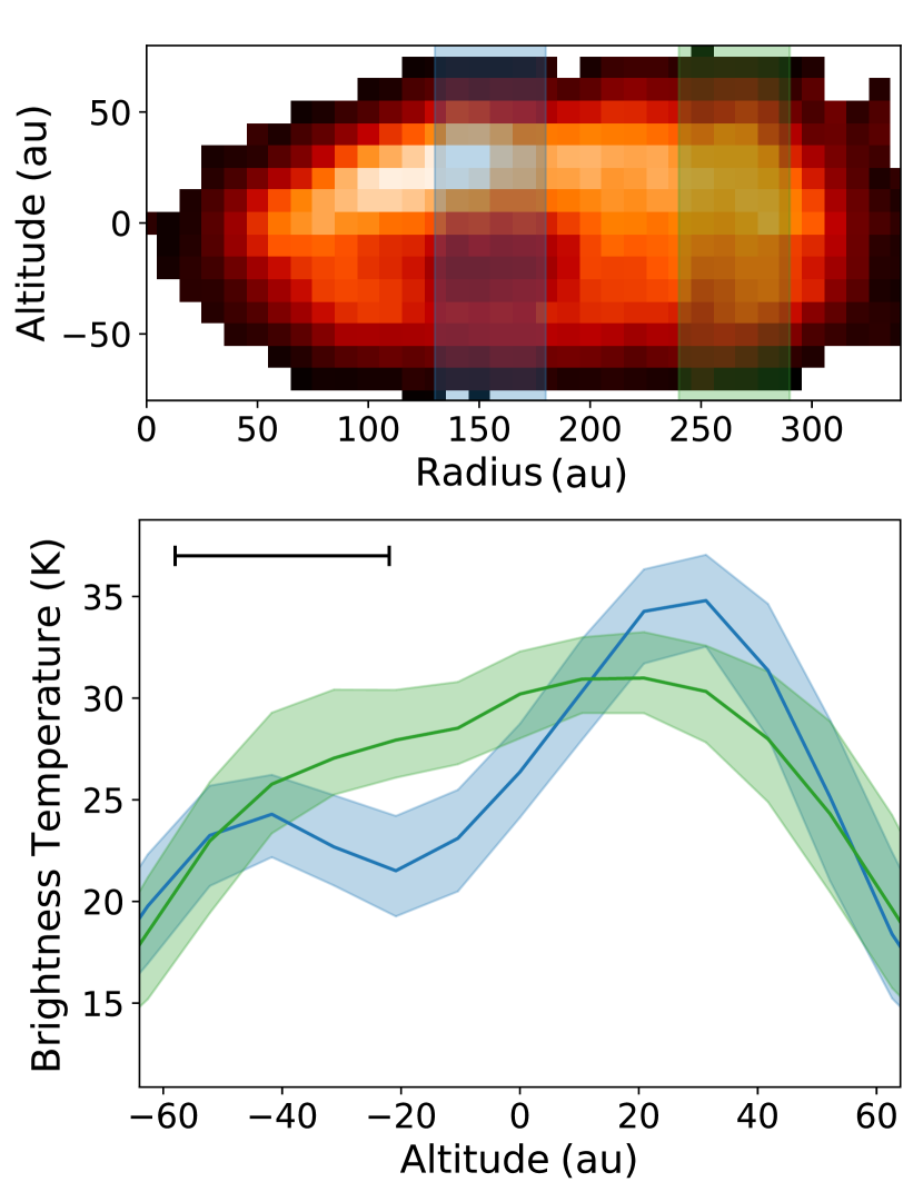
Figure 13: Top panel: left-right average of the ¹²CO temperature map. The two color shaded regions at distances of 135-175 (blue) and 245-285 (green) mark the distances where radial averages are performed. Bottom panel: temperature as a function of the disk’s altitude taken at 135-175 (blue) and 245-285 (green) as shown in the top panel. The shaded regions around the solid lines, correspond to the temperature uncertainties calculated from the maps. The horizontal bar shown in the bottom panel corresponds to the spatial resolution of 36 au in this direction.

Although it seems clear from Figure 11 that in ¹²CO there are a top and a bottom emitting layers separated by a colder midplane, the three pixel averaged profiles of Figure 12 suggest that the midplane is not significantly cooler than the bottom layer. We further investigate this ambiguity by looking at vertical temperature profiles of the ¹²CO map. As shown in Figure 13, we chose two regions to perform the vertical cuts, one region at a radial distance of $135-175$ au, and a second region at radial a distance of $245-285$ au. The first region was chosen to go through the cold midplane region in the disk (marked as a light blue region) while the second one was chosen to go through the outer disk (marked as a light green region). In the bottom panel of Figure 13, we show the temperature of the disk as a function of vertical distance above and below the midplane in the two regions marked above. The blue line clearly depicts the top and bottom emitting regions and the colder midplane zone mentioned before, with the midplane region being $\delta T=3\pm 2$ K cooler than the bottom region and $13\pm 2$ K cooler than the top region. This is qualitatively consistent with TRD maps of the Flying Saucer and Gomez’ Hamburger (Dutrey et al., 2017; Teague et al., 2020). The temperature structure changes significantly when the cut is performed towards the outer region. The green curve does not show a valley structure, which shows that the midplane temperature has increased at radial distances larger than $R\sim 200$ au, but there is still a marginal level of asymmetry showing that the top side of the disk still appears to be slightly warmer than the bottom side at larger distances from the center.

The temperature asymmetry between the top and bottom sides of the disk is an optical depth effect caused by a slight deviation out of edge-on inclination of Oph163131 coupled with the significant line optical depth and vertical thickness of the warm molecular layer. At the top of the disk ($z>0$), the optical depth $\tau=1$ is reached towards the disk’s surface, therefore providing the temperature of the disk’s high elevation layers which is warmer as it is directly exposed to the star. This effect is further amplified by the fact that, even at small deviations out of edge-on position, the far side of the disk, on the top side, becomes visible to the observer (even if the disk is not resolved), causing a larger area of the disk to be exposed to the observer and consequently artificially increasing the measured temperature (see Appendix B.2). On the bottom side ($z<0$ au) of the disk, however, the $\tau=1$ surface is reached closer to the midplane from the observer’s perspective, providing a temperature measurement of the disk’s lower elevation regions. Additionally, it is expected that at the locations where the dust continuum is optically thick, the gas emission could be absorbed, further lowering the brightness temperature. Given the geometry of the disk, this effect only plays a role in regions below the midplane ($z<0$). This is why even after the TRD technique transforms the disk into $R-Z$ coordinates, there is still a temperature asymmetry between the two sides of the disk.

The temperature asymmetry, combined with the angular resolution of the observations and the intrinsic angular scales of the Oph163131 disk, also explains the off-centered cold disk midplane (by approximately $-20$ au) shown in Figure 13. The more exposed CO upper emitting layer appears broader and hotter than the less-exposed CO bottom emitting layer, which causes the whole disk midplane to be shifted towards the bottom side of the disk (see also Figure 17 of the Appendix). All of the above is then amplified by the flux smearing induced by the spatial resolution of the observations. Finally, the close match between the temperature of the bottom ¹²CO emission and of the (symmetric) ¹³CO is consistent with observations of IM Lup (Pinte et al., 2018) and confirm a freeze-out temperature of $\sim$20 K.

5 Discussion

5.1 Oph163131 compared to other sources

We now put Oph163131 in context by comparing its properties against other sources with direct disk temperature measurements. We focus on four sources with well spectrally and spatially resolved ¹²CO observations, where a model-independent temperature measurement was performed: IM Lupi (Pinte et al., 2018), the Flying Saucer (Dutrey et al., 2017), Gomez’s Hamburger (Teague et al., 2020), and HD 163296 (Dullemond et al., 2020; Isella et al., 2018). Two of the sources (Gomez’s Hamburger and the Flying Saucer) harbor edge-on disks and have been analyzed using the TRD method in a very similar fashion as we have done here for Oph163131, therefore a full reconstructed temperature map is available for comparison. The other two sources (IM Lupi and HD 163296) have disks with intermediate inclination angles ($i\sim 45\arcdeg$) and report direct temperature measurements on specific parts of the disk (i.e., at the surface level or towards the midplane).

The central stars of these sources span a relatively large range of masses, Gomez’s Hamburger and HD 163296 are regarded as Herbig stars with stellar masses of $2.5\pm 0.5$ $\rm M_{\odot}$ (Teague et al., 2020) and $2.04^{+0.25}_{-0.14}$ $\rm M_{\odot}$ (Andrews et al., 2018), respectively. IM Lupi and the Flying Saucer, on the other hand, have stellar masses of $1.0\pm 0.1$ $\rm M_{\odot}$ and $0.58\pm 0.01$ $\rm M_{\odot}$, respectively, both consistent with being T Tauri stars, which make them better candidates to be compared against the disk of Oph163131. The much higher luminosity of Herbig stars should result in substantially higher temperatures throughout the disk (e.g., Kamp et al., 2011).

The maximum temperature measured from ¹²CO observations in the disks of the Herbig star’s Gomez’s Hamburger and HD 163296, reach values of $\sim 60$ K and $\sim 90$ K, respectively, which are significantly hotter than the temperatures measured in the T Tauri stars’ disks of $\sim 30$ K for IM Lupi and Oph163131, and of $\sim 20$ K in the disk of the less massive star Flying Saucer. Minimum temperatures of the disks are harder to compare as they strongly depend on where the temperatures are measured, how well resolved the disks are, and the sensitivity of the observations.

Pinte et al. (2018) produced radial temperature profiles computed from the ¹²CO and the ¹³CO lines for IM Lupi (their figure 4, right panel), which can be easily compared to our Figure 12. In ¹²CO, the maximum temperatures of the disks are 35 K and 32 K which are reached at distances of $\sim 150$ au and $\sim 190$ au for Oph163131 and IM Lupi, respectively. The temperature decline towards larger radii, however, is markedly shallower in Oph163131 than in IM Lupi: $\sim 2.5$ K per 100 au and $\sim 6$ K per 100 au, respectively. In ¹³CO, the radial profiles of both sources reach a plateau with peak values of 19 K and 21 K for Oph163131 and IM Lupi, with similar decreases towards the outermost regions of the disks. We note, however, that contrary to the IM Lupi study, our ¹³CO observations do not fully resolve the layers on either side of the midplane and, thus the ¹³CO temperature profile reported in our study is only a vertical average, making the comparison less straightforward.

For most of the sources mentioned above, we have estimated the ratio between the disk’s full vertical extent ($Z_{max}$) and total disk’s radial size ($R_{max}$) in ¹²CO. The thicker disk, using this metric, is the Flying Saucer with a ratio of $\frac{Z_{max}}{R_{max}}\sim 0.5$, IM Lupi and the Gomez’s Hamburger come next with a similar vertical to radial ratio of $\frac{Z_{max}}{R_{max}}\sim 0.33$, and finally the thinnest disk is Oph163131 with a ratio of $\frac{Z_{max}}{R_{max}}\sim 0.23$. In this comparison, we have excluded HD 163296, as the vertical size measurement performed on this disk is strongly model dependent and therefore not a fair comparison against the other sources (Isella et al., 2018).

Despite contrasting disks sizes of sources obtained at different spatial resolutions, these comparisons can provide some insights into how the stellar masses, evolution, and the temperature of the disks relate to the aspect ratio of the sources. For T Tauri stars, it appears that more massive stars correlate with thinner disks, although with only three sources in the sample, this result lacks statistical significance. An alternative view is that each disk could be in a different evolutionary state where vertical settling may have progressed by different amounts. In the case of Oph163131, the absence of strong accretion (see Section 3.1) means that there is much less UV radiation available to heat up the gas, which ultimately causes the flat aspect of this disk. Alcalá et al. (2017) measured an accretion luminosity of 0.08 $L_{\odot}$ for IM Lupi by modeling the excess emission from the UV to the near-infrared of X-shooter data. The excess of accretion radiation might explain the larger $\frac{Z_{max}}{R_{max}}$ value for IM Lupi when compared to Oph163131. As for the Flying Saucer, we have not found accretion measurements in the literature. HST images show no signs of any jet or molecular outflows in the vicinity of this source, yet this does not rule out stellar accretion.

The accretion status of other edge-on protoplanetary disks that have a low height to radius ratio and display flat parallel nebulae in scattered light images (as seen in Oph1613131) is discussed next. HK Tau B, a well studied edge-on disk (Koresko, 1998; Stapelfeldt et al., 1998), was classified as a CTTS by Monin et al. (1998), albeit with an optical spectrum that displays a modest $H_{\alpha}$ emission and no other emission line. The optical spectrum of LkH$\alpha$ 263C, a similarly flat disk (Jayawardhana et al., 2002; Chauvin et al., 2002), reveals that it has a strong $H_{\alpha}$ emission along with prominent forbidden emission lines. Finally ESO H$\alpha$ 574, another flat-shaped disk imaged with HST (Stapelfeldt et al., 2014), has a prominent optical jet, which suggests ongoing stellar accretion. In summary, flat shaped proplanetary disks are found around actively accreting and non-substantially accreting stars. We encourage a study that would quantify the accretion radiation and aspect ratio of disks to test whether accretion-induced UV radiation could significantly affect the vertical thickness of protoplanetary disks.

5.2 The inner disk: inside 200 au

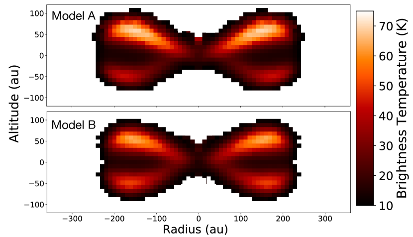
Figure 14: Comparison between the two temperature maps produced using the MCFOST synthetic models with parameters adopted from Paper I. The top panel corresponds to the temperature map obtained using the 0.8 µm  HST best fit parameters (Model A), and the bottom panel from ALMA 1.3 mm continuum parameters (Model B).

The reconstructed ¹²CO temperature map of Oph163131 shows two distinct regions with a demarcation at a radius of $\sim 200$ au. Inside of this radius, the CO emission arises from two elevated layers separated by a midplane, whereas the outer region consists of a much more vertically uniform emission. Interestingly, this radial break coincides with the outer radius at which both the submillimeter continuum emission and the scattered light are detected (see Figure 8 and also Villenave et al. (2020). We, therefore, address the “inner” and “outer” regions separately. Considering first the inner disk, we note that the observed behavior of the gas emission is similar to that observed in other disks (e.g., IM Lupi and The Flying Saucer discussed above). We now wish to go beyond qualitative comparisons and evaluate whether detailed radiative transfer models of the dust components of Oph163131 can reproduce the temperature structure we obtain from the gas.

In Paper I, ALMA 1.3 mm dust continuum observations and 0.8 µm  HST scattered light images of Oph163131 were modeled. To reproduce the observations, Paper  I uses the MCFOST radiative transfer code and a Markov Chain Monte Carlo (MCMC) approach to fit the millimeter and sub-micron data of Oph163131 independently. The individual fits, which assumed a tapered-edge surface density profile, provided a set of density and geometrical parameters of the disk such as inclination angle, scale height, surface density, flaring exponent, among others (see their Equation 1 and Table 4). In this section, we compare the models from Paper I to our ¹²CO reconstructed temperature map, limiting the analysis to the inner 200 au.

To perform a meaningful comparison, we took the following approach. We used Paper I dust disk density and geometrical parameters, a gas-to-dust ratio of 100, a CO/H₂ abundance of $10^{-4}$, and we imposed CO freeze out (CO/H₂ = 0) in regions where the temperature of the disk falls below 20 K. We then computed the synthetic ¹²CO J = 2 - 1 observations of such a disk with MCFOST. From the resulting data cubes, we analyze these models in the exact same manner as we did with gas observations in Section 4, i.e., using the same parameters for Oph163131 such as stellar mass, spatial and spectral resolution, distance to the star, etc. The two models we consider are a) a model that fits the HST 0.814 µm  image (Paper I’s model A) which has a disk inclination angle of $i=84.5\arcdeg$, a scale height of H₀ $=7.2$ au (at 100 au), and a critical radius of $R_{C}=89$ au, where $R_{C}$ has the usual meaning of the distance at which the disk surface density changes from a power-law to an exponential taper; and b) a model that reproduces the 1.3 millimeter continuum ALMA map (Paper I’s model B), with an inclination angle of $i=87.2\arcdeg$, a scale height of H₀ $=9.5$ au (at 100 au), and a critical radius of $R_{C}=74.5$ au. The model retrieved temperature maps are shown in Figure 14.

Both models produce a disk with clearly defined top and bottom CO emission layers separated by cold and frozen midplane. The maximum temperature of the gas, however, is almost twice as hot as the data, and the elevation of the CO layers in the 150 to 200 au radial range is also significantly higher (50 au) than the observations ($\sim 35$ au). This means that the parameters that reproduce sub-micron (Model A) and millimeter size (Model B) dust grains do not necessarily match the gas observations when adopting standard gas-to-dust and CO-to-$\rm H_{2}$ abundance ratios.

One possible path to reconcile the dust and gas observations is to reduce the overall CO gas mass in the disk. This would decrease the altitude at which the CO becomes optically thick and also the temperature of the emitting layer, as the gas is found at deeper layers in the disk. In practice, this means to either adopt a lower gas-to-dust ratio ($<100$) or a lower CO-to-$\rm H_{2}$ abundance ratio ($<10^{-4}$) in the disk. Ansdell et al. (2016) performed a large study of young stars in Lupus and found that most disks have gas-to-dust ratios of less than 100 for an assumed standard CO-to-$\rm H_{2}$ abundance ($10^{-4}$). Long et al. (2017) analyzed a large number of disks bearing sources in Chamaleon I and found median gas-to-dust ratios of $\sim 4-15$, depending on the assumptions made. Recent observations of individual disks have shown that CO could be depleted by several orders of magnitude with respect to H₂ (Favre et al., 2013; Kama et al., 2016; Trapman et al., 2017; Zhang et al., 2017, 2020). These anomalous abundances have been explored using physical and chemical models that deplete CO in disks (e.g., Bosman et al., 2018). In particular, Krijt et al. (2020) used models that combine chemical processing of CO with ice sequestration in the disk midplane to obtain strong CO depletion in the outer disk warm molecular layers.

Although there is extensive literature that suggests the possibility of a lower gas-to-dust ratio and CO-to-$\rm H_{2}$ abundance in disks, such ad-hoc adjustment in our models of Oph163131 does not necessarily provide a satisfactory match to the gas observations. One example of this is that using a lower gas-to-dust ratio would immediately affect the dust settling mechanism, and just like this, other backreactions could occur if lower CO-to-$\rm H_{2}$ abundances are adopted. As discussed in the next subsection, only detailed modeling of the CO observations would provide the appropriate physical parameters of the gas component of the disk around Oph163131.

5.3 The outer disk: outside 200 au

In subsection 4.3, we pointed out that the outer disk ($\rm R>200$ au) of Oph163131 has an almost constant temperature of $\sim$30 K at all elevations and radii. This is readily seen from panel c of Figure 12 where all three layers converge to a similar temperature, and in Figure 13 where the outer vertical temperature profile is almost flat-topped. This result is somewhat surprising in multiple ways. First of all, we did not observe this behavior in the tests performed on the synthetic disk models. In these tests, we varied the beam size and the disk inclination and yet always obtained a top and a bottom layer separated by a colder midplane (Appendix B), indicating that this is not a feature of the TRD technique. Therefore there appears to be an additional process that leads to a much more vertically uniform temperature than expected. Second, a sharp jump in temperature is inconsistent with typical trends as a function of distance from the central star. This indicates that there is an important transition in the disk properties at this location. Finally, the 30 K that is observed in the outer disk is much higher than the expected blackbody equilibrium temperature, which is about 20 K and 15 K at 200 and 300 au, respectively, assuming low-albedo dust grains. Since this temperature has a very shallow dependency on stellar luminosity, it is highly unlikely that this could be due to the star being much more luminous than we assumed in our models. This points to the gas being overheated compared to expectations. Here we speculate on a possible explanation for these behaviors.

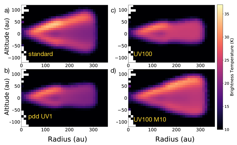
Figure 15: MCFOST models with external UV irradiation might explain the flat-topped outer regions of Oph163131 as well as the increased temperature towards the outer parts of the disk. Panel a) shows the generic model without external irradiation. Panel b) shows the generic model but we turn on photodissociation and photodesorption with an UV irradiation environment equal to solar. Panel c) shows a 100 times increased UV irradiation environment. Panel d) shows the generic model with 100 times the solar UV irradiation (same as c), but the mass of the outer disk is increased by a factor of 10.

The radial position where the midplane temperature of Oph163131 increases from 21 K to 30 K, coincides with the position where the millimeter continuum emission is no longer detected (R$\sim 200$ au, see Figure 8 and Paper I). A similar behavior is seen in the Flying Saucer Dutrey et al. (2017), in which a sharp (albeit smaller) temperature jump is observed at the outer radius of the millimeter continuum map. However, one significant difference between the two disks is that submicron dust is traced in scattered light out to much larger radii in the Flying Saucer, whereas in Oph163131 the radial extent of the millimeter continuum and scattered light images are very similar to one another (see Paper I). We speculate that the dust grain difference relates to the observed midplane temperature profile outside of the millimeter continuum: it is uniform for Oph163131 but gradually declining for the Flying Saucer.

Dutrey et al. (2017) proposed that this sharp temperature increase is related to a higher influx of UV radiation penetrating the disk from the outside, leading to enhanced thermal or direct CO desorption. This is supported by our observations of Oph163131. Broadly speaking, the depletion of dust in the outer disk leads to a lower optical depth and thus higher penetration of short wavelength radiation. This process is even more dramatic in the case of Oph163131 where even small dust grains, which have high UV opacity, are absent or rare in the outer disk. In this case, we expect interstellar photons to penetrate deeper in the disk and to deposit more heat, leading to an even more uniform temperature in that region.

The much reduced dust density could also play a role in the heating of the outer parts as the gas could be more decoupled from the dust, allowing it to remain at a higher temperature. Large dust grains are known to be the most efficient emitters of far-IR and sub-millimeter radiation, and without them, the outer disk cannot radiatively cool as efficiently as in the inner parts. In this regard, we note that Oph163131 is positioned between the L1689 and L1688 Ophiuchus molecular clouds, in a region of substantially lower dust and gas column density than the Flying Saucer (Lombardi et al., 2008; Ladjelate et al., 2020). The remarkably uniform and warm temperature of the outer region of Oph163113 could thus be the consequence of enhanced interstellar UV radiation coupled with much lower dust opacity.

To go beyond pure speculations, we computed MCFOST synthetic disk models to test this hypothesis. We used the stellar parameter derived for Oph163131 and used disk geometrical and density parameters that visually matched the full extent of the disk around Oph163131. None of these models are meant to reproduce the observations of the gas component of Oph163131 but to demonstrate the effects of a higher external UV flux on the disks. We first constructed a ‘standard’ model that consists of an inner region (R$<$170 au) with a dust mass of $10^{-3}$ $\rm M_{\odot}$ and an outer region with a dust mass of $10^{-6}$ $\rm M_{\odot}$ that extends from 170 au to 300 au. Both regions have a gas-to-dust ratio of 100, but the outer region contains only small grains (the maximum grain size was set to 10 µm). This last requirement comes from the lack of sub-mm dust emission detected for Oph163131 at distances $>$200 au (see Paper I and Villenave et al., 2020). Finally to perform a meaningful comparison to our results, we applied the TRD technique on this synthetic data, just as we did in Section 5.2

Figure 15 shows the TRD maps for above mentioned models. The first model (panel a) corresponds to the ‘standard model’, in which we did not include photodesorption or photodissociation of the CO molecule, as a purely illustrative exercise. This model shows two well separated top and bottom layers extending from the inner part of the disk and all the way to the outer disk. In this model, the temperature of the midplane in the outer parts is of the order of 17 K, while the top layer reaches a maximum temperature of 26 K, indicating a strong vertical gradient that is not seen in the data. In the second model (panel b), we show the same ‘standard’ model but now we have activated photodesorption and photodissociation in the model, and external illumination is implemented with a UV flux set to the UV field in the Solar neighborhood value (Draine & Bertoldi, 1996). We see from this model that the interstellar photons have eroded the upper and bottom layers of the disk, creating a vertically flatter outer disk. Although the temperature of the midplane in the outer regions is still of the order of 17 K, we notice that the temperature has an almost uniform value at all vertical elevations. The third model (panel c) is a variant of the same model where the UV irradiation field is 100 times stronger than the value in the Solar neighborhood. The increased irradiation field does not alter the shape of the disk any further but it homogeneously increases the temperature of the outer disk to 22 K. In this model, we see the distinctive feature of an outer disk’s midplane that is hotter than the inner disk’s midplane, i.e., a radial temperature increase in the midplane’s temperature at radii larger than $\sim 100$ au. Finally, in a fourth model (panel d), we used the same parameters as in the previous model, i.e., a UV flux 100 times the Solar neighborhood value, but we also increased the mass of the outer disk by a factor of 10, i.e., to $10^{-5}$ $\rm M_{\odot}$ in dust ($10^{-3}$ $\rm M_{\odot}$ in gas). As can be seen in Figure 15, the increased outer disk mass leads to self-shielding of the CO gas in the outer disk, producing the formation of distinct upper and lower layers, a colder midplane and an overall flared appearance of the outer disk. The temperature of the top layer increased to 28 K, but the midplane temperature decreased to 20 K. Although it is not shown in the figure, we tested models with an even larger UV irradiation field. By the time the outer disk reached a temperature of 30 K, the radiation in the models was so high (1000 times the Solar neighborhood value) that it causes the whole disk to increase in temperature.

In conclusion, we showed that photodissociation and photodesorption are processes that can explain the vertically flat outer part of a disk, due to the erosion of the low-density top and bottom layers, as long as the overall gas column density (equivalently, mass) in the outer layer remains quite low, requiring a sharp decrease in surface density at 170–200 au. The stripping of these layers produces in turn a vertically isothermal outer disk. In addition, when the UV irradiation field is increased (compared to Solar neighborhood values) it causes a rise in the temperature of the outer parts, allowing the possibility of having an outer disk midplane that is hotter than the inner disk midplane. Finally, we point out that to obtain optimal disk parameters for this source, it would be necessary to perform a detailed radiative transfer modeling of the CO, varying density and geometrical parameters, and including external UV irradiation along with photodesorption and photodissociation processes.

6 Conclusion

In this study, we present the first ALMA CO observations of the disk around Oph163131, as well as, the first optical and NIR spectroscopic observations of the central star. A summary of our results are as follows:

• We obtained optical and NIR low-resolution spectra (R$\sim 1000-2000$) of Oph163131 with the Goodman and SpeX spectrographs, respectively. By comparing the strengths of several absorption lines in both wavelength regions against appropriate stellar templates, we derived a spectral type of K4$\pm 1$ IV for the star.

• From the optical spectrum of Oph163131, we measured a $0.6\pm 0.1$ Å  equivalent width of the H$\alpha$ line. This measurement in addition to a null detection of the Br$\gamma$ or Pa$\beta$ emission lines indicates that Oph163131 is currently not accreting at an appreciable level. A detection of the He I line at 1.08 $\micron$, on the other hand, suggests that there might be either outflow activity or a very low accretion.

• We used the velocity pattern imprinted in the disk by the star to infer a dynamical mass for Oph163131. Assuming a distance of 147 pc and an inclination angle of $i=87\arcdeg$, we derived a stellar mass of $1.2\,\rm M_{\odot}$ for the central source with conservative upper and lower mass limits of $1.4\,\rm M_{\odot}$ and $1.0\,\rm M_{\odot}$, respectively.

• We have generalized the TRD method developed by Dutrey et al. (2017) to include non-perfectly edge-on disks. This generalization increases the number of disks that can be analyzed using this technique. In the Appendix, we have characterized some of the limitations of this method that can produce, for example, an apparent temperature decrease in the low density regions of the disk and a temperature increase of the top side of a disk (closest to the observer) in the presence of small inclinations.

• Using the tomographically reconstruction distribution method, we obtained a model-independent measurement of the temperature structure of the disk surrounding Oph163131. Towards the inner R$<$200 au regions of the disk, we detect two emission layers separated by a dark lane, that we interpret as the top and bottom parts of a highly inclined disk separated by a cold and probably frozen-out midplane.

• The colder midplane temperature of 21 K in the disk around Oph163131 increases to $\sim 30$ K for distances R$>200$ au. This temperature increment coincides with a decrease in the micron and millimeter size dust detection in the disk. MCFOST models with increased UV irradiation qualitatively match the temperature increase, as well as, the vertically thinner structure of the outer regions. We propose that external UV irradiation could heat up the gas component in the outer disk, as the interstellar photons can more easily penetrate regions where dust particles are not present.

Overall, the disk surrounding Oph163131 is markedly more compact along the vertical direction than other well-studied disks, in both its dust and gaseous components. Combined with strong evidence for dust settling, low- to absent accretion on the central star, and low-density, over-heated outer region, this suggests that the system is a relatively advanced state of evolution that warrant further analysis. In particular, detailed line radiative transfer modeling of the CO maps presented here and new observations focused on different molecular tracers could provide a thorough picture of the vertical temperature profile, from the midplane to the upper surface of the disk.

Appendix A Equations to perform the Temperature Reconstruction of a non-perfectly edge-on disk

In this section, we provide the equations that relate a protoplanetary disk’s velocity and geometrical coordinates as seen from an observer’s point of view to the velocity and geometrical coordinates in the disk’s coordinate system.

We define the disk’s spatial coordinates as $\{x,y,z\}$ and its velocity coordinates as $\{v_{x},v_{y},v_{z}\}$. An observer at a finite distance $d$ and whose line of sight is inclined at an angle $\alpha$ with respect to the disk’s midplane defines its own coordinate system $\{x^{\prime},y^{\prime},z^{\prime}\}$ and velocity coordinates $\{v_{x}^{\prime},v_{y}^{\prime},v_{z}^{\prime}\}$. Both coordinate systems are related by the following matrix transformation.

$$\begin{pmatrix}x^{\prime}\\ y^{\prime}\\ z^{\prime}\end{pmatrix}=\begin{pmatrix}1&0&0\\ 0&\cos{\alpha}&-\sin{\alpha}\\ 0&\sin{\alpha}&\cos{\alpha}\\ \end{pmatrix}\cdot\begin{pmatrix}x\\ y\\ z\end{pmatrix}$$ (A1)

We further assume that the disk is rotating at Keplerian speed $v=\sqrt{GM/r}$ and that the velocity component in the $y$ direction in the disk’s reference frame can be described as:

$$v_{y}=x\sqrt{\frac{\rm GM}{(\rho^{2}+z^{2})^{3/2}}}\quad;\quad\rho^{2}=x^{2}+y^{2}$$ (A2)

in the second part of equation (A2), $\rho$ represents the disk’s radial distance in cylindrical coordinates as viewed from the disk’s reference frame. We now combine equations (A1) and (A2) to derive the line of sight velocity of the disk from the observer’s perspective

$$v_{y}^{\prime} = v_{y}\cos{\alpha}-v_{z}\sin{\alpha}\quad;v_{z}=0$$ (A3)

$$v_{y}^{\prime} = x\sqrt{\frac{\rm GM}{(\rho^{2}+z^{2})^{3/2}}}\cos{\alpha}$$ (A4)

in the previous equation we assumed that the disk is not moving in the z-direction. We now would like to express the radial distance $\rho$ in the disk’s rest frame as a function of the observer’s coordinates $v_{y}^{\prime},x^{\prime},$ and $z^{\prime}$. From equations (A4) and (A1) we have

$$\rho^{2} = \left(\frac{x^{\prime 2}\rm{GM}\cos^{2}{\alpha}}{v_{y}^{\prime 2}}\right)^{2/3}-z^{2}$$ (A5)

$$\rho^{2} = \left(\frac{x^{\prime 2}\rm{GM}\cos^{2}{\alpha}}{v_{y}^{\prime 2}}\right)^{2/3}-(z^{\prime}\cos{\alpha}-y^{\prime}\sin{\alpha})^{2}$$ (A6)

which after some algebra we can write as:

$$\rho^{2}=x^{\prime 2}+\left(z^{\prime}\sin{\alpha}\pm\cos{\alpha}\sqrt{gm-(x^{\prime 2}+z^{\prime 2})}\right)^{2}$$ (A7)

with

$$gm=\left(\frac{x^{\prime 2}\rm{GM}\cos^{2}{\alpha}}{v_{y}^{\prime 2}}\right)^{2/3}$$ (A8)

we take the real and positive solution of $\rho$, appropriate for the radius in cylindrical coordinate.

We additionally solve for the vertical geometrical component $z$ from the disk’s coordinate system as a function of the observer’s coordinates. Using equation (A1), we have

$$z = z^{\prime}\cos{\alpha}-y^{\prime}\sin{\alpha}$$ (A9)

$$y^{\prime} = \frac{\sqrt{\rho^{2}-x^{\prime 2}}-z^{\prime}\sin{\alpha}}{\cos{\alpha}}$$ (A10)

which we combine to obtain

$$z = z^{\prime}\cos{\alpha}-\left(\sqrt{\rho^{2}-x^{\prime 2}}-z^{\prime}\sin{\alpha}\right)\tan{\alpha}$$ (A11)

Therefore, for a given point in the PV diagram ($x^{\prime}$,$V_{y}^{\prime}$ space) and for a given $\alpha$ angle and $z^{\prime}$ vertical position, we can use equations (A7) and (A11) to find the radial and vertical position of an emitting parcel of gas in the disk.

Appendix B TRD model testing

In order to understand the limitations of the TRD method, we performed several tests on synthetic disk models. MCFOST is a line and continuum radiative transfer code that can produce atomic and molecular line maps of complex structures such as protoplanetary disks. To create a synthetic disk model, MCFOST first computes the temperature structure of a model assuming one or several energy sources. Under the assumption that dust and gas are thermally coupled (LTE), MCFOST then calculates the intensity of a given atomic or molecular species, creating a line map that can be compared to observations. In our models, we assumed that the dominant source of energy is a single star with stellar parameters consistent with our results in Sections 3.1 and 3.2. We assumed a tapered-edge disk geometry following Panić et al. (2009) and Pinte et al. (2018) with density and geometrical parameters qualitatively consistent with the observations. We emphasize that none of the disk models presented in this section are meant to be good a fit to the ALMA observations but to provide an idea of how different parameters such as the beam size of the observations and the inclination angle of the disk affect the TRD method. In these test models, we do not include photodesorption nor photodissociation effects. In Table 1, we summarize the stellar and disk parameters we used to create the synthetic disk models.

B.1 The ideal model

The first synthetic model we created is a perfectly edge-on disk ($i$=90°) with an extremely high spatial resolution (0$\farcs$01 or 1.4 au) and a spectral resolution that matches our observations ($<0.25\rm kms^{-1}$). Although we tried models with higher spectral resolution (0.01 $\rm kms^{-1}$), we found no significant differences between these two. We applied the TRD technique to this synthetic disk and compared the reconstructed temperature map to the input temperature from MCFOST in Figure 16. The input MCFOST temperature and the reconstructed temperature maps are shown as black lines and color maps, respectively with uneven steps of 5, 10, and 20 K to better display both temperatures. From the figure, we see that the temperature input and the retrieved temperature follow each other very closely at almost all radii and specially towards low-elevations. The 15 K to 35 K temperature regions, for example, match at almost all radii and elevations. The hotter temperature of 55 K, on the other hand, start deviating from the retrieved temperatures for radii larger than 200 au. The difference between the computed and the input temperatures is due to a lower density (lower optical depth ultimately) of the gas, which happens at both, very high elevations and larges distances from the center of the disk. In both cases, the reconstructed temperature is lower than the actual temperature of the disk. This behavior is expected and it follows from the definition of brightness temperature, which is known to coincide with the kinetic temperature of the gas when the optical depth of a line is sufficiently large. However, it is important to note that the models presented here do not have any included noise, therefore the optically thinner gas, often missed in the observations due to S/N detection limits, might not present a problem when using the TRD technique.

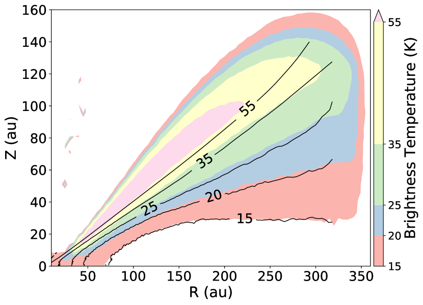
Figure 16: Comparison between the TRD method applied to the synthetic disk model and the input disk temperature parameters. The model (shown in colors) was created with the parameters defined in Table 1 and convolved with a 0$\farcs$01 beam. The MCFOST input temperature shown as black lines range from 15 K to 55 K.

Table 1: Disk and stellar parameters of the test model.

Model Parameter	Value
$a_{max}$   (µm)	1000
$\rm M_{dust}\,(M_{\odot})$	5.5 10-4
gas/dust	100
CO/H2	$10^{-4}$
$\beta$	1.25
$\gamma$	-1.0
$R_{c}$ (au)	40
$h$ (au)	15
M ($\rm M_{\odot}$)	1.2
L ($\rm L_{\odot}$)	0.96
$\rm T_{eff}$ (K)	4500

Note. — The scale height $h$ is measured at 100 au.

B.2 TRD with different disk inclinations

The probability of encountering a protoplanetary disk that is perfectly edge-on is very small. It is therefore important to consider the cases where there are small deviations in the inclination of the disk towards the observers. To explore what are the effects of inclining the disk’s out of edge-on position, we have computed two new MCFOST models with the same disk and stellar parameters as defined in Table 1 but this time we adopted inclinations of $i$=85°and $i$=80°.

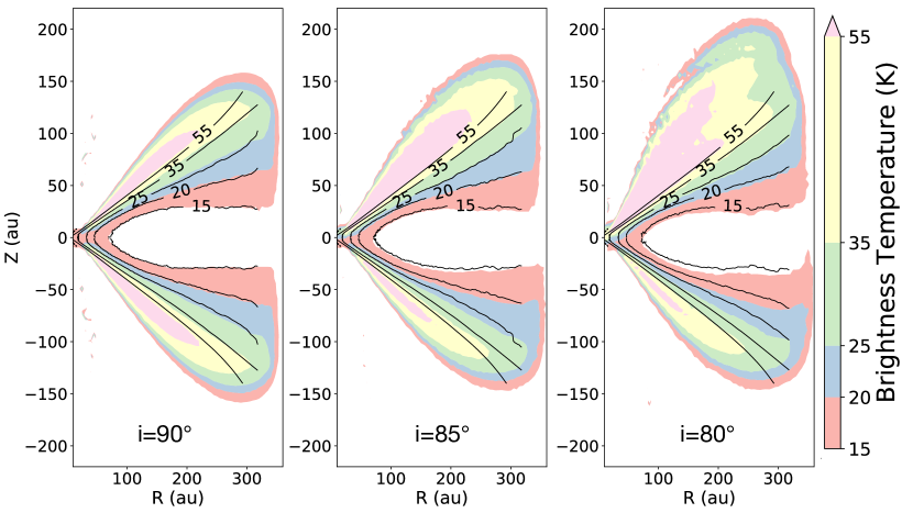
Figure 17: Demonstration of the disk inclination variation when using the TRD method. From left to right we plotted the synthetic disk at inclination angles of $i=90\arcdeg$, $i=85\arcdeg$, and $i=80\arcdeg$. The disks apparent temperature change with changing inclination in both, the layers above and below the midplane. Black contours lines correspond to the input MCFOST temperature.

In Figure 17, we plotted these two new models with inclinations of $i$=85°(middle) and $i$=80°(right panel), in addition to the default model with $i$=90°(left panel). This time both sides of the disk were plotted so the inclination effects can be visualized for the regions above and below the midplane. For the regions above the midplane, we see that as the disk is declined out of edge-on position, the far side of the disk becomes visible and lies above the photosphere of the disk overlapping with the near side. When the disk is inclined at $i$=85°, it is not possible to easily distinguish between the far and the near side of the disk in the reconstructed temperature map, so the emission from the far side is mixed with the emission from the photosphere on the near side, resulting in an increase on the measured temperature at higher elevations and also an increase in the scale height at all radii. When the disk is further declined to $i$=80°, the near and far side of the disk are clearly separated and the measured peak temperature returns to its original value. The layers below the midplane are also affected by changes in inclination. As the disk goes from $i=90\arcdeg$ to $i=80\arcdeg$ the near side gets hidden behind the disk’s midplane causing that the light emitted from the bottom layer arises from a place closer to the midplane (because of optical depth effects) and therefore we see a cooler temperature.

Although the TRD technique takes into consideration the inclination angle of the disk, the temperature reconstruction is affected by optical depth. This means, for example, that for a disk that is inclined at $i=80\arcdeg$, the layer further from the observer (bottom layer in our Figure 17) would not appear to be as hot as the closer layer (top layer), and this is not because the reconstruction is imperfect, instead this relates to the position in the disk where the optical depth of the line becomes much greater than unity. The same effect also causes that one side of the disk (top and bottom layers) appears to be larger than the other one. Although it might seem like that from Figure 17, the reality is that we compare different temperature contours, which are arbitrarily selected. If one would allow the temperatures to range from much lower to much higher values, then the disk’s would have the same sizes, but there would be temperature differences between them.

B.3 TRD with different spatial resolution

Now we turn to the problem of how the spatial resolution affects the reconstructed temperature distribution of a protoplanetary disk. We use the same disk parameter as in the previous section (see Table 1) and keep the inclination to $i$=90°. To simulate observations at different spatial resolutions, we convolved the synthetic disk model with a two dimensional circular Gaussian profile with a FWHM that varies from 0$\farcs$01 to 0$\farcs$3.

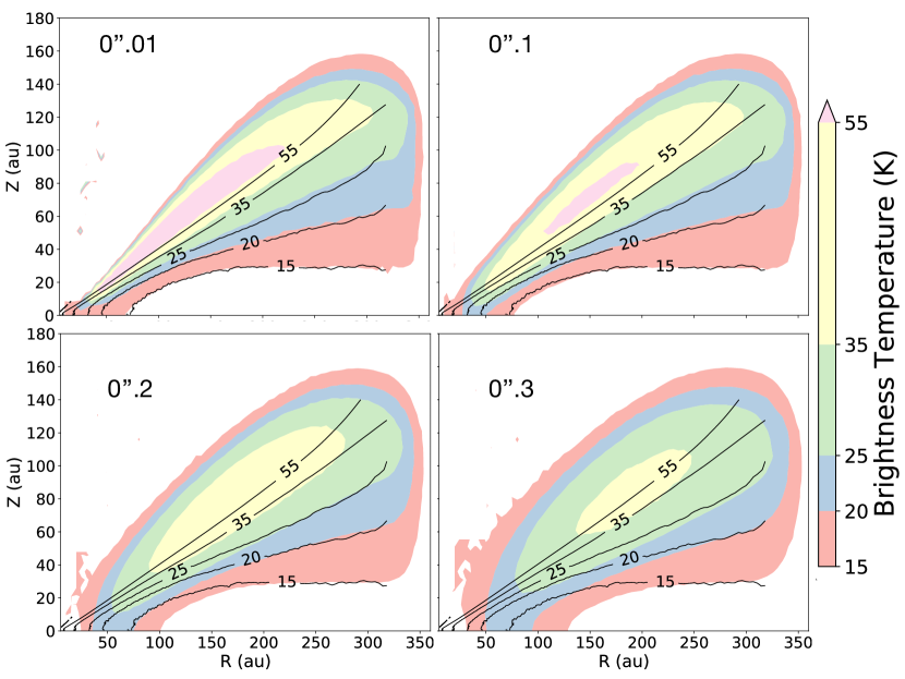
Figure 18: Comparison between temperature retrieved model convolved with different beam sizes. The top left panel shows a model convolved with a 0$\farcs$01 beam (same as Figure 16). Top right, bottom left, and bottom right panels show the same model convolved with a 0$\farcs$1, 0$\farcs$2, and 0$\farcs$3 beam sizes, respectively. Contours correspond to the input MCFOST temperature.

The spatial resolution effect is the most important limitation in our study of the temperature structure of a disk. It smears out the flux of the disk, limiting our ability to detecting high temperature regions confined in small scale structures. In Figure 18, we illustrate this effect by convolving the same model shown in Figure 16 with different synthetic beam sizes. As we convolve the models with larger beam sizes, the retrieved peak temperature decreases, and the small scale emission layers disappear. When the spatial resolution of the observations is degraded, the retrieved peak temperature shifts towards the center of the disk. Additionally, the disk appears to be thicker in the vertical direction extending beyond the nominal disk’s photosphere and also it becomes thicker towards the bottom part of the disk, where most of the CO has frozen-out. When the spatial resolution of the observations (for a disk of this size) is better than 0$\farcs$1, the convolution effects are much milder and the retrieved temperature is comparable to the true temperature in the disk. It must be kept in mind, however, that even for very high spatial resolution observations, there are practical limits on the resolution of the reconstruction temperature maps. As the TRD method depends on the average of multiple pixels at a given radial position, on the shear Keplerian velocity, and on the turbulent velocity of the disk (as explained in Section 4)

To conclude, we would like to emphasize that if the spatial resolution of the observations is poor enough, the beam smearing effect largely exceeds the inclination effects. With the data we have presented, we have to acknowledge that inside of 125 au – 150 au, we are likely to be affected by this effect, however, the outer disk is much less affected.

References

- Alcalá et al. (2014) Alcalá, J. M., Natta, A., Manara, C. F., et al. 2014, A&A, 561, A2, doi: 10.1051/0004-6361/201322254
- Alcalá et al. (2017) Alcalá, J. M., Manara, C. F., Natta, A., et al. 2017, A&A, 600, A20, doi: 10.1051/0004-6361/201629929
- Allen & Strom (1995) Allen, L. E., & Strom, K. M. 1995, AJ, 109, 1379, doi: 10.1086/117370
- Andrews (2020) Andrews, S. M. 2020, ARA&A, 58, 483, doi: 10.1146/annurev-astro-031220-010302
- Andrews et al. (2018) Andrews, S. M., Huang, J., Pérez, L. M., et al. 2018, ApJ, 869, L41, doi: 10.3847/2041-8213/aaf741
- Ansdell et al. (2016) Ansdell, M., Williams, J. P., van der Marel, N., et al. 2016, ApJ, 828, 46, doi: 10.3847/0004-637X/828/1/46
- Ansdell et al. (2018) Ansdell, M., Williams, J. P., Trapman, L., et al. 2018, ApJ, 859, 21, doi: 10.3847/1538-4357/aab890
- Appenzeller et al. (2005) Appenzeller, I., Bertout, C., & Stahl, O. 2005, A&A, 434, 1005, doi: 10.1051/0004-6361:20042217
- Astropy Collaboration et al. (2018) Astropy Collaboration, Price-Whelan, A. M., Sipőcz, B. M., et al. 2018, AJ, 156, 123, doi: 10.3847/1538-3881/aabc4f
- Avenhaus et al. (2018) Avenhaus, H., Quanz, S. P., Garufi, A., et al. 2018, ApJ, 863, 44, doi: 10.3847/1538-4357/aab846
- Barrado y Navascués & Martín (2003) Barrado y Navascués, D., & Martín, E. L. 2003, AJ, 126, 2997, doi: 10.1086/379673
- Barrière-Fouchet et al. (2005) Barrière-Fouchet, L., Gonzalez, J. F., Murray, J. R., Humble, R. J., & Maddison, S. T. 2005, A&A, 443, 185, doi: 10.1051/0004-6361:20042249
- Beckwith & Sargent (1993) Beckwith, S. V. W., & Sargent, A. I. 1993, ApJ, 402, 280, doi: 10.1086/172131
- Birnstiel & Andrews (2014) Birnstiel, T., & Andrews, S. M. 2014, ApJ, 780, 153, doi: 10.1088/0004-637X/780/2/153
- Bosman et al. (2018) Bosman, A. D., Walsh, C., & van Dishoeck, E. F. 2018, A&A, 618, A182, doi: 10.1051/0004-6361/201833497
- Boyden & Eisner (2020) Boyden, R. D., & Eisner, J. A. 2020, ApJ, 894, 74, doi: 10.3847/1538-4357/ab86b7
- Chauvin et al. (2002) Chauvin, G., Ménard, F., Fusco, T., et al. 2002, A&A, 394, 949, doi: 10.1051/0004-6361:20021215
- Christiaens et al. (2014) Christiaens, V., Casassus, S., Perez, S., van der Plas, G., & Ménard, F. 2014, ApJ, 785, L12, doi: 10.1088/2041-8205/785/1/L12
- Cieza et al. (2019) Cieza, L. A., Ruíz-Rodríguez, D., Hales, A., et al. 2019, MNRAS, 482, 698, doi: 10.1093/mnras/sty2653
- Cleeves et al. (2016) Cleeves, L. I., Öberg, K. I., Wilner, D. J., et al. 2016, ApJ, 832, 110, doi: 10.3847/0004-637X/832/2/110
- Cox et al. (2017) Cox, E. G., Harris, R. J., Looney, L. W., et al. 2017, ApJ, 851, 83, doi: 10.3847/1538-4357/aa97e2
- Cushing et al. (2004) Cushing, M. C., Vacca, W. D., & Rayner, J. T. 2004, PASP, 116, 362, doi: 10.1086/382907
- Dong et al. (2016) Dong, R., Fung, J., & Chiang, E. 2016, ApJ, 826, 75, doi: 10.3847/0004-637X/826/1/75
- Doppmann et al. (2005) Doppmann, G. W., Greene, T. P., Covey, K. R., & Lada, C. J. 2005, AJ, 130, 1145, doi: 10.1086/431954
- Draine & Bertoldi (1996) Draine, B. T., & Bertoldi, F. 1996, ApJ, 468, 269, doi: 10.1086/177689
- Duchêne et al. (2017) Duchêne, G., Becker, A., Yang, Y., et al. 2017, MNRAS, 469, 1783, doi: 10.1093/mnras/stx852
- Dullemond et al. (2020) Dullemond, C. P., Isella, A., Andrews, S. M., Skobleva, I., & Dzyurkevich, N. 2020, A&A, 633, A137, doi: 10.1051/0004-6361/201936438
- Dutrey et al. (2017) Dutrey, A., Guilloteau, S., Piétu, V., et al. 2017, A&A, 607, A130, doi: 10.1051/0004-6361/201730645
- Edwards et al. (2006) Edwards, S., Fischer, W., Hillenbrand, L., & Kwan, J. 2006, ApJ, 646, 319, doi: 10.1086/504832
- Evans et al. (2009) Evans, Neal J., I., Dunham, M. M., Jørgensen, J. K., et al. 2009, ApJS, 181, 321, doi: 10.1088/0067-0049/181/2/321
- Facchini et al. (2017) Facchini, S., Birnstiel, T., Bruderer, S., & van Dishoeck, E. F. 2017, A&A, 605, A16, doi: 10.1051/0004-6361/201630329
- Falcón-Barroso et al. (2011) Falcón-Barroso, J., Sánchez-Blázquez, P., Vazdekis, A., et al. 2011, A&A, 532, A95, doi: 10.1051/0004-6361/201116842
- Favre et al. (2013) Favre, C., Cleeves, L. I., Bergin, E. A., Qi, C., & Blake, G. A. 2013, ApJ, 776, L38, doi: 10.1088/2041-8205/776/2/L38
- Feiden (2016) Feiden, G. A. 2016, A&A, 593, A99, doi: 10.1051/0004-6361/201527613
- Fischer et al. (2008) Fischer, W., Kwan, J., Edwards, S., & Hillenbrand , L. 2008, ApJ, 687, 1117, doi: 10.1086/591902
- Flores et al. (2019) Flores, C., Connelley, M. S., Reipurth, B., & Boogert, A. 2019, ApJ, 882, A75, doi: 10.3847/1538-4357/ab35d4
- Flores et al. (2020) Flores, C., Reipurth, B., & Connelley, M. S. 2020, ApJ, 898, 109, doi: 10.3847/1538-4357/ab9e67
- Folha & Emerson (2001) Folha, D. F. M., & Emerson, J. P. 2001, A&A, 365, 90, doi: 10.1051/0004-6361:20000018
- Gonzalez et al. (2017) Gonzalez, J. F., Laibe, G., & Maddison, S. T. 2017, MNRAS, 467, 1984, doi: 10.1093/mnras/stx016
- Guilloteau et al. (2016) Guilloteau, S., Piétu, V., Chapillon, E., et al. 2016, A&A, 586, L1, doi: 10.1051/0004-6361/201527620
- Hsieh & Lai (2013) Hsieh, T.-H., & Lai, S.-P. 2013, ApJS, 205, 5, doi: 10.1088/0067-0049/205/1/5
- Huélamo et al. (2015) Huélamo, N., de Gregorio-Monsalvo, I., Macias, E., et al. 2015, A&A, 575, L5, doi: 10.1051/0004-6361/201424404
- Isella et al. (2018) Isella, A., Huang, J., Andrews, S. M., et al. 2018, ApJ, 869, L49, doi: 10.3847/2041-8213/aaf747
- Jacoby et al. (1984) Jacoby, G. H., Hunter, D. A., & Christian, C. A. 1984, ApJS, 56, 257, doi: 10.1086/190983
- Jayawardhana et al. (2002) Jayawardhana, R., Luhman, K. L., D’Alessio, P., & Stauffer, J. R. 2002, ApJ, 571, L51, doi: 10.1086/341202
- Kama et al. (2016) Kama, M., Bruderer, S., van Dishoeck, E. F., et al. 2016, A&A, 592, A83, doi: 10.1051/0004-6361/201526991
- Kamp et al. (2011) Kamp, I., Woitke, P., Pinte, C., et al. 2011, A&A, 532, A85, doi: 10.1051/0004-6361/201016399
- Koresko (1998) Koresko, C. D. 1998, ApJ, 507, L145, doi: 10.1086/311694
- Krijt et al. (2020) Krijt, S., Bosman, A. D., Zhang, K., et al. 2020, ApJ, 899, 134, doi: 10.3847/1538-4357/aba75d
- Ladjelate et al. (2020) Ladjelate, B., André, P., Könyves, V., et al. 2020, A&A, 638, A74, doi: 10.1051/0004-6361/201936442
- Le Borgne et al. (2003) Le Borgne, J. F., Bruzual, G., Pelló, R., et al. 2003, A&A, 402, 433, doi: 10.1051/0004-6361:20030243
- Lombardi et al. (2008) Lombardi, M., Lada, C. J., & Alves, J. 2008, A&A, 489, 143, doi: 10.1051/0004-6361:200810070
- Long et al. (2017) Long, F., Herczeg, G. J., Pascucci, I., et al. 2017, ApJ, 844, 99, doi: 10.3847/1538-4357/aa78fc
- Manara et al. (2013) Manara, C. F., Testi, L., Rigliaco, E., et al. 2013, A&A, 551, A107, doi: 10.1051/0004-6361/201220921
- Mannings & Sargent (1997) Mannings, V., & Sargent, A. I. 1997, ApJ, 490, 792, doi: 10.1086/304897
- McMullin et al. (2007) McMullin, J. P., Waters, B., Schiebel, D., Young, W., & Golap, K. 2007, in Astronomical Society of the Pacific Conference Series, Vol. 376, Astronomical Data Analysis Software and Systems XVI, ed. R. A. Shaw, F. Hill, & D. J. Bell, 127
- Monin et al. (1998) Monin, J. L., Menard, F., & Duchene, G. 1998, A&A, 339, 113
- Ortiz-León et al. (2017) Ortiz-León, G. N., Loinard, L., Kounkel, M. A., et al. 2017, ApJ, 834, 141, doi: 10.3847/1538-4357/834/2/141
- Panić et al. (2009) Panić, O., Hogerheijde, M. R., Wilner, D., & Qi, C. 2009, A&A, 501, 269, doi: 10.1051/0004-6361/200911883
- Pavlyuchenkov et al. (2007) Pavlyuchenkov, Y., Semenov, D., Henning, T., et al. 2007, ApJ, 669, 1262, doi: 10.1086/521872
- Perez et al. (2015) Perez, S., Casassus, S., Ménard, F., et al. 2015, ApJ, 798, 85, doi: 10.1088/0004-637X/798/2/85
- Pinte et al. (2009) Pinte, C., Harries, T. J., Min, M., et al. 2009, A&A, 498, 967, doi: 10.1051/0004-6361/200811555
- Pinte et al. (2006) Pinte, C., Ménard, F., Duchêne, G., & Bastien, P. 2006, A&A, 459, 797, doi: 10.1051/0004-6361:20053275
- Pinte et al. (2018) Pinte, C., Ménard, F., Duchêne, G., et al. 2018, A&A, 609, A47, doi: 10.1051/0004-6361/201731377
- Pinte et al. (2019) Pinte, C., van der Plas, G., Ménard, F., et al. 2019, Nature Astronomy, 3, 1109, doi: 10.1038/s41550-019-0852-6
- Rayner et al. (2009) Rayner, J. T., Cushing, M. C., & Vacca, W. D. 2009, ApJS, 185, 289, doi: 10.1088/0067-0049/185/2/289
- Rayner et al. (2003) Rayner, J. T., Toomey, D. W., Onaka, P. M., et al. 2003, PASP, 115, 362, doi: 10.1086/367745
- Sánchez-Blázquez et al. (2006) Sánchez-Blázquez, P., Peletier, R. F., Jiménez-Vicente, J., et al. 2006, MNRAS, 371, 703, doi: 10.1111/j.1365-2966.2006.10699.x
- Simon et al. (2019) Simon, M., Guilloteau, S., Beck, T. L., et al. 2019, ApJ, 884, 42, doi: 10.3847/1538-4357/ab3e3b
- Sokal et al. (2018) Sokal, K. R., Deen, C. P., Mace, G. N., et al. 2018, ApJ, 853, 120, doi: 10.3847/1538-4357/aaa1e4
- Somers & Pinsonneault (2015) Somers, G., & Pinsonneault, M. H. 2015, ApJ, 807, 174, doi: 10.1088/0004-637X/807/2/174
- Stapelfeldt et al. (2014) Stapelfeldt, K. R., Duchêne, G., Perrin, M., et al. 2014, in IAU Symposium, Vol. 299, Exploring the Formation and Evolution of Planetary Systems, ed. M. Booth, B. C. Matthews, & J. R. Graham, 99–103, doi: 10.1017/S1743921313008004
- Stapelfeldt et al. (1998) Stapelfeldt, K. R., Krist, J. E., Ménard, F., et al. 1998, ApJ, 502, L65, doi: 10.1086/311479
- Teague et al. (2020) Teague, R., Jankovic, M. R., Haworth, T. J., Qi, C., & Ilee, J. D. 2020, MNRAS, 495, 451, doi: 10.1093/mnras/staa1167
- Thanathibodee et al. (2018) Thanathibodee, T., Calvet, N., Herczeg, G., et al. 2018, ApJ, 861, 73, doi: 10.3847/1538-4357/aac5e9
- Trapman et al. (2017) Trapman, L., Miotello, A., Kama, M., van Dishoeck, E. F., & Bruderer, S. 2017, A&A, 605, A69, doi: 10.1051/0004-6361/201630308
- Vacca et al. (2003) Vacca, W. D., Cushing, M. C., & Rayner, J. T. 2003, PASP, 115, 389, doi: 10.1086/346193
- Villenave et al. (2020) Villenave, M., Ménard, F., Dent, W. R. F., et al. 2020, A&A, 642, A164, doi: 10.1051/0004-6361/202038087
- Woitke et al. (2019) Woitke, P., Kamp, I., Antonellini, S., et al. 2019, PASP, 131, 064301, doi: 10.1088/1538-3873/aaf4e5
- Zhang et al. (2017) Zhang, K., Bergin, E. A., Blake, G. A., Cleeves, L. I., & Schwarz, K. R. 2017, Nature Astronomy, 1, 0130, doi: 10.1038/s41550-017-0130
- Zhang et al. (2015) Zhang, K., Blake, G. A., & Bergin, E. A. 2015, ApJ, 806, L7, doi: 10.1088/2041-8205/806/1/L7
- Zhang et al. (2020) Zhang, K., Schwarz, K. R., & Bergin, E. A. 2020, ApJ, 891, L17, doi: 10.3847/2041-8213/ab7823