Interpolation of surfaces with asymptotic curves in Euclidean 3-space

Abstract

In this paper, we investigate the interpolation of surfaces which are obtained from an isoasymptotic curve in 3D-Euclidean space. We prove that there exist a unique $C^{0}$-Hermite surface interpolation related to an isoasymptotic curve under some special conditions on the marching scale functions. Finally, we present some examples and plot their graphs.

1 Introduction

Differential geometry is a branch of mathematics which uses advanced calculus tools in geometry. In recent years, it has become an applicable area of mathematics in science and technology. Since the manifold theory has used in general relativity in the 1900s by Einstein, differential geometry of curves, surfaces and general manifolds have been improving more. Notably, from medicine to social science and from artificial intelligence to economy, it is very clear how the differential geometry is applied. In this manner, one can consider that the applied mathematics has been changed from numerical and computational methods to differential geometrical tools. For example, to understand the meaning of multiple features data we use calculus on manifolds in machine learning [5]. Also, differential geometry permit us to work on non-euclidean spaces as most real life problems are define in such spaces. So, it is a fundamental tool for understanding events in the universe.

A relevant kind of curves is geodesics which play the role of straight lines in Euclidean space on a manifold. Gauss proved that the differential geometry of a surface is different from the geometry of ambient space. The well known example of supporting these ideas is that a geodesic on a unit sphere embedded in a Euclidean space is not a geodesic in a Euclidean space. In this way, the differential geometry of a surface has many significant properties that we can use in applied sciences. The minimal distance between two points on a surface is called a geodesic and this is considered as an important idea in many applications [4, 12].

A surface could be constructed using a geodesic. In [23] a general surface is obtained from a polynomial geodesic. Also, considering a 3-dimensional polynomial curve which is a pregeodesic, the authors constructed ruled cubic patched in [21]. In addition, in [19] authors investigated a developable surface that contains a given Bezier geodesic. Wang at al. defined a parametric surface which is called surface family, using a geodesic curve [26]. They used the Frenet frame of the curve and presented necessary conditions in which the curve is an isogeodesic on a parametric surface considering Frenet aparatus of the curve. The methods in this paper is a reverse of some engineering problems. Later, Kasap et al. [14] generalized their methods and presented examples. Li et al. studied the approximation minimal surface with geodesics by using the Dirichlet function and they minimized the area of a surface family by using Dirichlet approach. This method can be used for obtaining the minimal cost of the material while building surfaces. The family surfaces have been studied for example as in [13, 14, 1, 2, 27, 28].

The other special curve which is as important as geodesics is the asymptotic curves. An asymptotic curve is a curve always tangent to an asymptotic direction of the surface and it has zero normal curvature. On the other hand, one can be constructed a surface using an asymptotic curve. Saad et al. [22] approximated the minimal parametric surface with an asymptotic curve by minimizing the Dirichlet function. In [20] they examined rational developable surface pencils through an arbitrary parametric curve as its common asymptotic curve. Moreover, Güler at al. constructed a surface interpolating a given curve as the asymptotic curve of it [11]. Similar to geodesics, the asymptotic curves also have many applications in related sciences. In [24] the authors presented a method to design strained grid structures along asymptotic curves to benefit from a high degree of simplification in fabrication and construction. Also, asymptotic curves has many applications in astronomy as in [7, 10].

Lee et al. [15] introduced a new method to construct a parametric surface in terms of curves. They defined a surface interpolation associated with a spatial curve passing through some $m$-points in Euclidean $3$-space. Motivating all studies mentioned from here, we consider a surface interpolation using asymptotic curves in Euclidean space. We organized this paper as follow: We give some fundamental facts which are used throughout the paper, in Section 2. Section 3 is devoted to the surface interpolations with isoparametric curve and examples with their graphs.

2 Preliminaries

In this section, we give a short review on curves and surfaces in an 3D-Euclidean space. For details we refer the reader to any classical differential geometry books, for example [25].

Let $\gamma(\omega)$ be a curve which is arc-length $\omega$ in 3D Euclidean space. Take the Frenet frame of $\gamma(\omega)$ by $\left\{\mathcal{V}_{1}(\omega),\mathcal{V}_{2}(\omega),\mathcal{V}_{3}(\omega)\right\}$. Then we have the following well known relations between $\kappa(\omega)$ and $\tau(\omega)$ are the curvature and the torsion of the curve $\gamma(\omega)$, respectively.

$$\left[\begin{array}[c]{c}{\mathcal{V}_{1}}^{{}^{\prime}}(\omega)\\ {\mathcal{V}_{2}}{{}^{\prime}}(\omega)\\ {\mathcal{V}_{3}}^{{}^{\prime}}(\omega)\end{array}\right]=\left[\begin{array}[c]{ccc}0&\kappa(\omega)&0\\ -\kappa(\omega)&0&\tau(\omega)\\ 0&-\tau(\omega)&0\end{array}\right].\left[\begin{array}[c]{c}\mathcal{V}_{1}(\omega)\\ \mathcal{V}_{2}(\omega)\\ \mathcal{V}_{3}(\omega)\end{array}\right]$$

.

Previous equations are called the Frenet apparatus of a curve and they are important to understand the geometry of the curve. Also, we can classify curves via the Frenet–Serret frames. In [26] Wang et al. defined pencil surface which could be obtained using the Frenet–Serret frames of the curve. This surface is called by a surface family or a pencil surface and it is defined as follows.

Definition 1.

Let $\gamma(\omega)$ be a curve which is arc-length $\omega$ in $\mathbb{E}^{3}$ and $\left\{\mathcal{V}_{1}(\omega),\mathcal{V}_{2}(\omega),\mathcal{V}_{3}(\omega)\right\}$ be the Frenet frame of $\gamma$. Then the map

$$\Psi(\omega,\eta)=\gamma(\omega)+u(\omega,\eta)\cdot\mathcal{V}_{1}(\omega)+v(\omega,\eta)\cdot\mathcal{V}_{2}(\omega)+z(\omega,\eta)\cdot\mathcal{V}_{3}(\omega),$$ (1)

is defined a surface in $\mathbb{E}^{3}$, where $\Omega\geq\omega\geq 0,\Lambda\geq\eta\geq 0$ for a real-valued constants $\Omega,\Lambda$, and  $u(\omega,\eta),v(\omega,\eta)$ and $z(\omega,\eta)$ are $C^{1}-$functions. The surface $\Psi(\omega,\eta)$ is called as surface family or pencil surface [26].

By the following definition we classify some special curves on a parametric surface $\Psi(\omega,\eta)$.

Definition 2.

Lets take a curve $\gamma(s)$ on a parametric surface $X(s,\eta)$. Then we have following characterizations [25]:

1. $\gamma(s)$ is said to be an isoparametric curve on $X(s,\eta)$ if there exists a parameter $\eta_{0}\in[0,\Lambda]$ such that $X(s,\eta_{0})=\gamma(s).$

2. $\gamma(s)$ is an asymptotic curve on a parametric surface $X(s,\eta)$ if $\frac{\partial\mathcal{N}(s,\eta_{0})}{\partial s}.\mathcal{V}_{1}(s)=0,$ where $\mathcal{N}(s,\eta)$ is the normal vector of surface $X(s,\eta)$, $\mathcal{V}_{1}(s)$ is the tangent vector of curve $\gamma(s)$.

3. $\gamma(s)$ is called isoasymptotic of the surface $X(s,\eta)$ if it is both a asymptotic curve and an isoparametric curve on the surface $X(s,\eta)$.

With following theorem we have the necessary and sufficient conditions for $\gamma$ to be isoasymptotic curve on the surface $\Psi(\omega,\eta)$ (1).

Theorem 3.

[3] Let $\Psi(\omega,\eta)$ be a parametric surface with the marching-scale functions;

$$u(\omega,\eta) =k(\omega)U(\eta),$$

$$v(\omega,\eta) =m(\omega)V(\eta),$$

$$z(\omega,\eta) =n(\omega)Z(\eta),$$

where $k(\omega),U(\eta),m(\omega),V(\eta),n(\omega)$ and $Z(\eta)$ are $C^{1}-$functions. Then $\gamma(\omega)$ is an isoasymptotic curve on a parametric surface $\Psi(\omega,\eta)$ (1) if and only if we have

$$\left\{\begin{array}[c]{c}U(\eta_{0})=V(\eta_{0})=Z(\eta_{0})=0,\\ n(\omega)=0\text{ or }\frac{\partial Z(\eta_{0})}{\partial\eta}=0.\end{array}\right.$$ (2)

If we take $k(\omega)=m(\omega)=n(\omega)=1$ ,particularly and consider $U(\eta)$, $V(\eta)$ and $Z(\eta)$ as polynomials of the forms in (2), then we have

$$U(\eta) =\sum\limits_{t=1}^{n}a_{t}(\eta-\eta_{0})^{t},$$ (3)

$$V(\eta) =\sum\limits_{t=1}^{n}b_{t}(\eta-\eta_{0})^{t},$$

$$Z(\eta) =\sum\limits_{t=1}^{n}c_{t}(\eta-\eta_{0})^{t},\text{ \ }c_{1}=0,$$

respectively, where $a_{t},b_{t},c_{t}$ are constant. Then the polynomials $U(\eta)$, $V(\eta)$ and $Z(\eta)$ in (3) satisfy the isoasymptotic condition (2). Thus, we can determine marching-scale functions of a surface family $\Psi(\omega,\eta)$ by the polynomial expressions.

3 Surface Interpolations with Isoasymptotic Curve

In this section, we construct a surface with isogeodesic curve passing through finite control points lying on $\mathbb{E}^{3}.$

Now, we give a definition for surface interpolations with isoasymptotic curve passing through some control points on $\mathbb{E}^{3}.$

Definition 4.

Let $A_{1},A_{2},...,A_{m}$ be different points on $\mathbb{E}^{3}$ and $\Psi(\omega,\eta):B\subset\mathbb{R}^{2}\rightarrow\mathbb{E}^{3}$ be a parametric pencil surface given by (1). For some different points $(\omega_{t},\eta_{t})\in B$ $(t=1,...,m),$ we can construct the surface $\Psi(\omega,\eta)$ such that $\Psi(\omega_{t},\eta_{t})=A_{t}$. It is called a surface interpolation associated with the given isoasymptotic curve $\gamma(\omega)$ passing through $m$-control points $A_{t}~{}(t=1,...,m)$, simply, $C^{0}-$Hermite surface interpolation with an isoasymptotic curve. In particular, $\left\{A_{1},A_{2},...,A_{m}\right\}$ is called $C^{0}$-Hermite data.

Polynomials $U(\eta)$, $V(\eta)$ and $Z(\eta)$ with degree $n$ in (3) have $n,n$ and $n-1$ degrees of freedom in terms of coeffcients $a_{t},b_{t}$ and $c_{t}$ respectively. In this case, there are two extra degrees of freedom. To determine a unique parametric surface with isoasymptotic curve, we may assume $a_{n}=b_{n}=0$.

Now, we consider an isoasymptotic curve on surface parametrization

$$\Psi(\omega,\eta)=\gamma(\omega)+U(\eta)\cdot\mathcal{V}_{1}(\omega)+V(\eta)\cdot\mathcal{V}_{2}(\omega)+Z(\eta)\cdot\mathcal{V}_{3}(\omega),$$ (4)

$$\Omega\geq\omega\geq 0,\text{ \ \ \ \ \ \ }\Lambda\geq\eta\geq 0,\text{\ \ }$$

with the marching-scale functions are given in (3) for $a_{n}=b_{n}=0.$

Theorem 5.

Let $A_{1},A_{2},...,A_{m}$ be different points on a parametric surface $\Psi(\omega,\eta)$ given in (4). For $\Psi(\omega_{t},\eta_{t})=A_{t},t=1,...,m$ there exists a unique $C^{0}$-Hermite surface interpolation with an isoasymptotic curve such that the marching-scale functions are given by

$$U(\eta)=\sum\limits_{t=1}^{n-1}a_{t}(\eta-\eta_{0})^{t},\ \ V(\eta)=\sum\limits_{t=1}^{n-1}b_{t}(\eta-\eta_{0})^{t}\ \ \text{and }Z(\eta)=\sum\limits_{t=2}^{n}c_{t}(\eta-\eta_{0})^{t},$$

and

$$det\left(\begin{array}[c]{ccccc}d_{12}&\eta_{1}-\eta_{0}&(\eta_{1}-\eta_{0})^{2}&\cdots&(\eta_{1}-\eta_{0})^{n-1}\\ d_{22}&\eta_{2}-\eta_{0}&(\eta_{2}-\eta_{0})^{2}&\cdots&(\eta_{2}-\eta_{0})^{n-1}\\ \vdots\vdots&\vdots&\ddots&\vdots\\ d_{n2}&\eta_{n-1}-\eta_{0}&(\eta_{n-1}-\eta_{0})^{2}&\cdots&(\eta_{n-1}-\eta_{0})^{n-1}\end{array}\right)$$

where $a_{t},b_{t}$ and $c_{t}$ are constant and $d_{t2}=V(\eta_{t2}),\ t=1,2,\ldots,n$.

Proof.

Let us define $(n-1)$-points of the surface $\Psi(\omega_{t},\eta_{t})$ by

$$\Psi(\omega_{t},\eta_{t})=A_{t}\text{ for }\omega\geq\eta_{n-1}...\geq\eta_{1}\geq\eta_{0}\geq 0.\text{ }$$

So, we have $\Psi(\omega_{t},\eta_{t})=A_{t}=\gamma(\omega_{t})+\mathcal{V}_{1}(\omega_{t}).U(\eta_{t})+\mathcal{V}_{2}(\omega_{t}).V(\eta_{t})+\mathcal{V}_{3}(\omega_{t}).Z(\eta_{t})$. By taking inner product with $\mathcal{V}_{1}(\omega)$, $\mathcal{V}_{2}(\omega)$, and $\mathcal{V}_{3}(\omega)$, respectively we obtain the coefficients as following

$$U(\eta_{t}) =\left\langle A_{t}-\gamma(\omega_{t}),\mathcal{V}_{1}(\omega_{t})\right\rangle,$$

$$V(\eta_{t}) =\left\langle A_{t}-\gamma(\omega_{t}),\mathcal{V}_{2}(\omega_{t})\right\rangle,$$

$$Z(\eta_{t}) =\left\langle A_{t}-\gamma(\omega_{t}),\mathcal{V}_{3}(\omega_{t})\right\rangle.$$

Using

$$U(\eta_{t})=d_{t1},\text{ }V(\eta_{t})=d_{t2},\text{ }Z(\eta_{t})=d_{t3}$$

where $d_{t1}$, $d_{t2}$ and $d_{t3}$ are constant, from (3) for $a_{n}=b_{n}=0,$ we have following matrices;

$$\left(\begin{array}[c]{cccc}\eta_{1}-\eta_{0}&(\eta_{1}-\eta_{0})^{2}&\cdots&(\eta_{1}-\eta_{0})^{n-1}\\ \eta_{2}-\eta_{0}&(\eta_{2}-\eta_{0})^{2}&\cdots&(\eta_{2}-\eta_{0})^{n-1}\\ \vdots&\vdots&\ddots&\vdots\\ \eta_{n-1}-\eta_{0}&(\eta_{n-1}-\eta_{0})^{2}&\cdots&(\eta_{n-1}-\eta_{0})^{n-1}\end{array}\right)\left(\begin{array}[c]{c}a_{1}\\ a_{2}\\ \vdots\\ a_{n-1}\end{array}\right)=\left(\begin{array}[c]{c}d_{11}\\ d_{21}\\ \vdots\\ d_{(n-1)1}\end{array}\right),$$

$$\left(\begin{array}[c]{cccc}\eta_{1}-\eta_{0}&(\eta_{1}-\eta_{0})^{2}&\cdots&(\eta_{1}-\eta_{0})^{n-1}\\ \eta_{2}-\eta_{0}&(\eta_{2}-\eta_{0})^{2}&\cdots&(\eta_{2}-\eta_{0})^{n-1}\\ \vdots&\vdots&\ddots&\vdots\\ \eta_{n-1}-\eta_{0}&(\eta_{n-1}-\eta_{0})^{2}&\cdots&(\eta_{n-1}-\eta_{0})^{n-1}\end{array}\right)\left(\begin{array}[c]{c}b_{1}\\ b_{2}\\ \vdots\\ b_{n-1}\end{array}\right)=\left(\begin{array}[c]{c}d_{12}\\ d_{22}\\ \vdots\\ d_{(n-1)2}\end{array}\right),$$

$$\left(\begin{array}[c]{cccc}(\eta_{1}-\eta_{0})^{2}&(\eta_{1}-\eta_{0})^{3}&\cdots&(\eta_{1}-\eta_{0})^{n}\\ (\eta_{2}-\eta_{0})^{2}&(\eta_{2}-\eta_{0})^{3}&\cdots&(\eta_{2}-\eta_{0})^{n}\\ \vdots&\vdots&\ddots&\vdots\\ (\eta_{n-1}-\eta_{0})^{2}&(\eta_{n-1}-\eta_{0})^{3}&\cdots&(\eta_{n-1}-\eta_{0})^{n}\end{array}\right)\left(\begin{array}[c]{c}c_{2}\\ c_{3}\\ \vdots\\ c_{n}\end{array}\right)=\left(\begin{array}[c]{c}d_{13}\\ d_{23}\\ \vdots\\ d_{(n-1)3}\end{array}\right),$$

for $1\leq\eta\leq n-1$. Lets take

$$M_{1} =\left(\begin{array}[c]{cccc}\eta_{1}-\eta_{0}&(\eta_{1}-\eta_{0})^{2}&\cdots&(\eta_{1}-\eta_{0})^{n-1}\\ \eta_{2}-\eta_{0}&(\eta_{2}-\eta_{0})^{2}&\cdots&(\eta_{2}-\eta_{0})^{n-1}\\ \vdots&\vdots&\ddots&\vdots\\ \eta_{n-1}-\eta_{0}&(\eta_{n-1}-\eta_{0})^{2}&\cdots&(\eta_{n-1}-\eta_{0})^{n-1}\end{array}\right)$$

and

$$M_{2} =\left(\begin{array}[c]{cccc}(\eta_{1}-\eta_{0})^{2}&(\eta_{1}-\eta_{0})^{3}&\cdots&(\eta_{1}-\eta_{0})^{n}\\ (\eta_{2}-\eta_{0})^{2}&(\eta_{2}-\eta_{0})^{3}&\cdots&(\eta_{2}-\eta_{0})^{n}\\ \vdots&\vdots&\ddots&\vdots\\ (\eta_{n-1}-\eta_{0})^{2}&(\eta_{n-1}-\eta_{0})^{3}&\cdots&(\eta_{n-1}-\eta_{0})^{n}\end{array}\right).$$

Then the determinants of $M_{1}$ and $M_{2}$ is obtained as

$$\det(M_{1}) =(-1)^{\frac{(n-1)(n-2)}{2}}\prod\limits_{t=1}^{n-1}(\eta_{t}-\eta_{0})\prod\limits_{1\leq t<j\leq n-1}(\eta_{t}-\eta_{j}),$$

and

$$\det(M_{2})=(-1)^{\frac{(n-1)(n-2)}{2}}\prod\limits_{t=1}^{n-1}(\eta_{t}-\eta_{0})^{2}\prod\limits_{1\leq t<j\leq n-1}(\eta_{t}-\eta_{j}).$$

Since $\eta_{t}$ and $\eta_{j}$ are non-zero and different from each others, for $1\leq t<j\leq n-1$, we get $\det(M_{1})\neq 0$ and $\det(M_{1})\neq 0$, that is, $a_{1},a_{2}$, …,$a_{n-1},$ $b_{1},b_{2}$, …,$b_{n-1}$ and $c_{2},c_{3}$, …,$c_{n}$ have unique solutions. This gives us that there exists a uniquely $C^{0}$-Hermite surface interpolation with an isoasymptotic curve. ∎

Example 6.

Consider a curve parametrized by

$$\gamma(\omega)=(\frac{\sin\omega}{2},\frac{\cos\omega}{2},\frac{\sqrt{3}\omega}{2}),\text{ \ \ \ \ \ }0\leq\omega\leq 2\pi.$$ (5)

The curve (5) is shown in Figure 1. By a direct computation, we have

$$\mathcal{V}_{1}(\omega) =(\frac{\cos\omega}{2},-\frac{\sin\omega}{2},\frac{\sqrt{3}}{2}),$$

$$\mathcal{V}_{2}(\omega) =(-\sin\omega,-\cos\omega,0),$$

$$\mathcal{V}_{3}(\omega) =(\frac{\sqrt{3}\cos\omega}{2},-\frac{\sqrt{3}\sin\omega}{2},\frac{-1}{2})$$

For $A_{1}=(1,7,\frac{\sqrt{3}\pi}{4})$, the point $A_{1}$ lies on the surface pencil with an isoasymptotic curve given by (4). If we take

$$U(\eta)=a_{1}\eta,\text{ }V(\eta)=b_{1}\eta,\text{ }W(\eta)=c_{2}\eta^{2}$$

then there is only one surface with an isoasymptotic curve passing the point $A_{1}.$ We take $\omega_{1}=\frac{\pi}{2},$ $\eta_{1}=2,$ i.e., $\Psi_{1}(\frac{\pi}{2},2)=A_{1}(1,7,\frac{\sqrt{3}\pi}{4})$ We obtain the equations:

$$\frac{1}{2}-2b_{1} =1,$$

$$-a_{1}-2\sqrt{3}c_{2} =7,$$

$$\sqrt{3}a_{1}-c_{2} =0,$$

which imply

$$a_{1}=-1,\text{ }b_{1}=-\frac{1}{2},\text{ }c_{2}=-\sqrt{3}.$$

Thus, we can construct the surface with an isoasymptotic curve passing the one point $A_{1}=(1,7,\frac{\sqrt{3}\pi}{4})$ given by

$$\Psi_{1}(\omega,\eta) =\frac{1}{2}(\sin(\omega)-3\eta^{2}\cos(\omega)+\eta\sin(\omega)-\eta\cos(\omega),$$ (6)

$$(\eta^{2}+\eta)\sin(\omega)+(\eta+1)\cos(\omega),\sqrt{3}(\omega+\eta^{2}-\eta))$$

The surface (6) is shown in Figure 2 and  the surface (6) with curve (5) is shown in Figure 3.

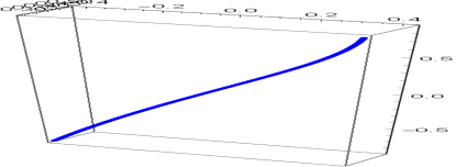
Figure 1: Graph of $\gamma$

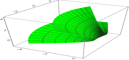
Figure 2: Graph of surface $\Psi_{1}$ is cunstructued by $\gamma$

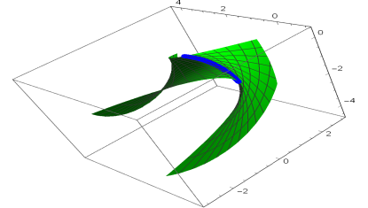
Figure 3: Graph of surface $\Psi_{1}$ with curve $\gamma$

Example 7.

Let the surface with an isoasymptotic curve above Example pass through the additional point $A_{2}=(\frac{1}{2},0,\frac{\sqrt{3}\pi}{4})$. For the convenience of calculations, taking $\omega_{2}=\frac{\pi}{2},$ $\eta_{2}=1,$ we have $A_{2}(\frac{1}{2},0,\frac{\sqrt{3}\pi}{4})$ and obtain the system of linear equations as follows:

$$b_{1}+2b_{2} =-\frac{1}{4},$$

$$a_{1}+2a_{2}+2\sqrt{3}(c_{2}+2c_{3}) =-7,$$

$$\sqrt{3}(a_{1}+2a_{2}) =2(c_{2}+2c_{3}),$$

$$b_{1} =-b_{2},$$

$$-(a_{1}+a_{2}) =\sqrt{3}(c_{2}+c_{3}),$$

$$\sqrt{3}(a_{1}+a_{2}) =c_{2}+c_{3}.$$

So, we obtain

$$b_{1} =\frac{1}{4},\text{ }b_{2}=-\frac{1}{4},\text{ }c_{2}=\frac{7\sqrt{3}(3-\sqrt{3})}{12},~{}c_{2}=\frac{7\sqrt{3}(\sqrt{3}-3)}{12},$$

$$a_{1} =\frac{14(3-\sqrt{3})}{12},~{}a_{2}=\frac{14(\sqrt{3}-3)}{12}.$$

Thus the surface with an isoasymptotic curve passing the two points $A_{1}=(1,7,\frac{\sqrt{3}\pi}{4})$ and $A_{2}(\frac{1}{2},0,\frac{\sqrt{3}\pi}{4})$ is uniquely given by

$$\Psi_{2}(\omega,\eta) =(\frac{\sin(\omega)}{2}+\frac{7\left(3-\sqrt{3}\right)}{12}\left(\eta-\eta^{2}\right)\cos(\omega)$$

$$-\frac{\sin(\omega)}{4}\left(\eta-\eta^{2}\right)+\frac{7\left(3-\sqrt{3}\right)}{8}\left(\eta^{2}-\eta^{3}\right)\cos(\omega),$$

$$\frac{\cos(\omega)}{2}-\frac{7\left(3-\sqrt{3}\right)}{12}\left(\eta-\eta^{2}\right)\sin(\omega)$$ (7)

$$-\left(\eta-\eta^{2}\right)\frac{\cos(\omega)}{4}-\frac{7\left(3-\sqrt{3}\right)}{8}\left(\eta^{2}-\eta^{3}\right)\sin(\omega)+,$$

$$\frac{\sqrt{3}s}{2}+\frac{7\left(\sqrt{3}-1\right)}{4}\left(\eta-\eta^{2}\right)-\frac{7\left(\sqrt{3}-1\right)}{8}\left(\eta^{2}-\eta^{3}\right)).$$

The surface (7) is shown in Figure 4 and  the surface (7) with curve (5) is shown in Figure 5.

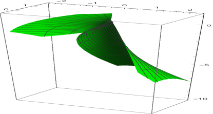
Figure 4: Graph of surface $\Psi_{2}$

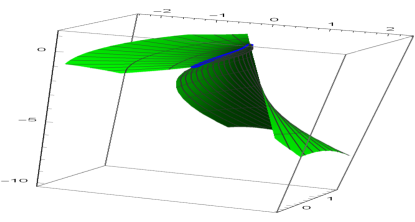
Figure 5: Graph of surface $\Psi_{2}$ with curve $\gamma$

References

• [1] Atalay, G.Ş. and Kasap, E. Family of surface with a common null geodesic, International Journal of Physical Sciences 4(8) (2009) 428-433.
• [2] Atalay, G.Ş. and Kasap, E. Surfaces family with common null asymptotic, Applied Mathematics and Computation 260 (2015) 135-139.
• [3] Bayram, E., Güler, F., and Kasap, E. Parametric representation of a surface pencil with a common asymptotic curve. Computer-Aided Design, 44(7),(2012), 637-643.
• [4] Brémond R., Jeulin D. , Gateau P. ,Jarrin J. , and Serpe G. , Estimation of the transport properties of polymer composites by geodesic propagation, J. Microsc. 176 (1994)
• [5] Bronstein, M. M., Bruna, J., LeCun, Y., Szlam, A., and Vandergheynst, P. Geometric deep learning: going beyond euclidean data. IEEE Signal Processing Magazine, 34(4), (2017), 18-42.
• [6] Che W. , Paul J-C. and Zhang X. Lines of curvature and umbilical points for implicit surfaces, Computer Aided Geometric Design 24(7) (2007) 395-409.
• [7] Contopoulos, G. Asymptotic curves and escapes in Hamiltonian systems. Astronomy and Astrophysics,(1990), 231, 41-55.
• [8] Ergün E. , Bayram E. and Kasap, E. Surface pencil with a common line of curvature in Minkowski 3-space, Acta Mathematica Sinica, English Series 30.12 (2014) 2103-2118.
• [9] Ergün E. , Bayram E. and Kasap, E. Surface family with a common natural line of curvature lift, Journal of Science and Arts 15(4) (2015) 321.
• [10] Efthymiopoulos, C., Contopoulos, G., and Voglis, N. Cantori, islands and asymptotic curves in the stickiness region. In Impact of Modern Dynamics in Astronomy, (1999) (pp. 221-230). Springer, Dordrecht.
• [11] Güler, F. Şaffak Atalay G., Gülnur E. and Kasap E. An approach for designing a surface pencil through a given asymptotic curve, Journal of Applied Mathematics and Computation (JAMC), 2019, 3(4), 606-615
• [12] Haw R. J. , An application of geodesic curves to sail design, Comput. Gragh. Forum 4 (1985), 137-139.
• [13] Kasap, E. and Akyildiz, F.T. Surfaces with common geodesic in Minkowski 3-space, Applied mathematics and computation 177(1) (2006) 260-270.
• [14] Kasap E., Akyildiz, F.T. and Orbay, K. A generalization of surfaces family with common spatial geodesic, Applied Mathematics and Computation 201(1-2) (2008) 781-789.
• [15] Lee H.C, Lee J.W, and Won D. Yoon Interpolation of Surfaces With Geodesics, J. Korean Math. Soc. 57 (2020), No. 4, pp. 957-971
• [16] Li, C-Y., Wang, R-H. and Zhu, C-G Parametric representation of a surface pencil with a common line of curvature, Computer-Aided Design 43(9) (2011) 1110-1117.
• [17] Li, C-Y., Wang, R-H. and Zhu, C-G A generalization of surface family with common line of curvature, Applied Mathematics and Computation 219(17) (2013) 9500-9507.
• [18] Li, C-Y., Wang, R-H. and Zhu, C-G Designing approximation minimal parametric surfaces with geodesics. Applied mathematical modelling, 37(9) (2013) 6415-6424.
• [19] Li, C.-Y., Wang, R.-H. and Zhu, C.-G. Design and $G^{1}$ connection of developable surfaces through Bézier geodesics, Appl. Math. Comput. 218 (2011), no. 7, 3199-3208.
• [20] Liu, Y., and Wang, G. J. Designing developable surface pencil through given curve as its common asymptotic curve. Journal of Zhejiang University (Engineering Science),(2013) 47(7), 1246-1252.
• [21] M. Paluszny, Cubic polynomial patches through geodesics, Comput. Aided Des. 40 (2008), 56-61. manizing Digital Reality (pp. 125-140). Springer, Singapore.
• [22] Saad, M. K., Abdel-Baky, R. A., Alharbi, F., and Aloufi, A. (2019). On Minimal Surfaces with the Same Asymptotic Curve in Euclidean Space. Applied Mathematical Sciences, 13(21), 1021-1031.
• [23] J. Sánchez-Reyes and R. Dorado, Constrained design of polynomial surfaces from geodesic curves, Comput. Aided Des. 40 (2008), 49-55.
• [24] Schling, E., Hitrec, D., and Barthel, R. (2018). Designing grid structures using asymptotic curve networks. In Hu
• [25] Struik, D.J. Lectures on classical differential geometry. Courier Corporation (1961).
• [26] Wang, G-J., Tang, K. and Tai, C-L. Parametric representation of a surface pencil with a common spatial geodesic, Computer-Aided Design 36(5) (2004) 447-459.
• [27] Z.K. Yüzbaşı and M. Bektaş, On the construction of a surface family with common geodesic in Galilean space G3, Open Physics 14(1) (2016) 360-363.
• [28] Z.K. Yüzbası, On a family of surfaces with common asymptotic curve in the Galilean space G3, J. Nonlinear Sci. Appl 9 (2016) 518-523.