Optical Spin Conductivity in Ultracold Quantum Gases

Abstract

We show that the optical spin conductivity being a small AC response of a bulk spin current and elusive in condensed matter systems can be measured in ultracold atoms. We demonstrate that this conductivity contains rich information on quantum states by analyzing experimentally achievable systems such as a spin-1/2 superfluid Fermi gas, a spin-1 Bose-Einstein condensate, and a Tomonaga-Luttinger liquid. The obtained conductivity spectra being absent in the Drude conductivity reflect quasiparticle excitations and non-Fermi liquid properties. Accessible physical quantities include the superfluid gap and the contact for the superfluid Fermi gas, gapped and gapless spin excitations as well as quantum depletion for the Bose-Einstein condensate, and the spin part of the Tomonaga-Luttinger liquid parameter elusive in cold-atom experiments. Unlike its mass transport counterpart, the spin conductivity serves as a probe applicable to clean atomic gases without disorder and lattice potentials. Our formalism can be generalized to various systems such as spin-orbit coupled and nonequilibrium systems.

I Introduction

Transport plays crucial roles in understanding states of matter in and out of equilibrium and paves the way to application such as control of matter and device fabrication. In solid state physics, the main bearer of transport is an electron and the properties of the electric current have conventionally been investigated mermin . Subsequently, the spin current being a flow of electric spin has attracted attention since the discovery of the giant magnetoresistance binasch ; baibich and the tunneling magnetoresistance miyazaki . More recently, due to the progress in nanofabrication technology of devices, physics in spin currents maekawa has also been widespread over materials with spin-Hall effects sinova , and topological insulators qi .

One of the hot topics in the rapid growth of the spintronics is to measure AC spin currents in a direct manner heinrich ; woltersdorf ; matsuo ; jiao ; sun ; hahn ; wei ; weiler ; li ; kobayashi ; kurimune . Such AC currents are detected in junction systems, and the determination of an AC conductivity of bulk spin transport is difficult in solid state systems. To address this spin transport property, we shed light on ultracold atoms being an ideal platform for quantum simulation of many-body systems schafer . Recently, the cold-atom analog of electronics referred to as atomtronics has attracted widespread attention amico , and transport measurements with ultracold atoms have been done with bulk ott ; strohmaier ; Sommer:2011a ; Sommer:2011b ; Jepsen:2020 ; Bardon:2014 ; Hild:2014 ; Koschorreck:2013 ; schneider ; ronzheimer ; heinze ; scherg ; brown ; nichols ; Anderson:2019 and mesoscopic setups krinner . One of the advantages of ultracold atoms is that spin-selective manipulation and probe are allowed, which opens up the possibility of precise measurements of spin transport enss-thywissen .

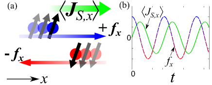
Figure 1: (a) Schematic image for probing the optical spin conductivity $\sigma_{\alpha\beta}^{(S)}(\omega)$ in ultracold atomic gases with spin $S=1/2$. The AC spin current $\langle J_{S,x}(t)\rangle$ is induced by a spin-dependent driving forces $\pm f_{x}(t)$. (b) Time evolutions of $f_{x}(t)=F_{x}\cos(\omega_{0}t)$ and the induced spin current, which is related to $\sigma_{xx}^{(S)}(\omega=\omega_{0})$ by $\langle J_{S,x}(t)\rangle/F_{x}=\mathrm{Re}\,\sigma_{xx}^{(S)}(\omega_{0})\cos(\omega_{0}t)+\mathrm{Im}\,\sigma_{xx}^{(S)}(\omega_{0})\sin(\omega_{0}t)$ resulting from Eq. (VI).

In this paper, we propose that ultracold atoms provide us with a simple way to measure an optical spin conductivity $\sigma_{\alpha\beta}^{(S)}(\omega)$, which characterizes an AC response of bulk spin transport. The spectrum of $\sigma_{\alpha\beta}^{(S)}(\omega)$ includes richer information on bulk properties than its DC limit related to spin diffusion, which has been actively studied Sommer:2011a ; Sommer:2011b ; Jepsen:2020 ; Bardon:2014 ; Hild:2014 ; Koschorreck:2013 ; enss-thywissen ; Bulchandani:2021 . This paper is organized as follows: In Sec. II, we provide the formalism of $\sigma_{\alpha\beta}^{(S)}(\omega)$ applicable to both continuum and optical lattice systems. We then demonstrate the availability of $\sigma_{\alpha\beta}^{(S)}(\omega)$ by investigating experimentally verifiable systems. Specifically, a spin-1/2 superfluid Fermi gas, a spin-1 Bose-Einstein condensate (BEC), and a Tomonaga-Luttinger (TL) liquid are studied in Secs. III, IV, and V, respectively. Reflecting on nontrivial spin excitations, these systems show interesting transport properties being absent in the conventional Drude conductivity. Section VI is devoted to proposing a method to measure $\sigma_{\alpha\beta}^{(S)}(\omega)$ from an oscillating behavior in spin dynamics as shown in Fig. 1. Prospects towards spin-orbit coupled and nonequilibrium systems in Sec. VII and other promising applications in Sec. VIII suggest that $\sigma^{(S)}_{\alpha\beta}(\omega)$ may be the Rosetta stone to unravel spin dynamics of various quantum many-body systems. We conclude in Sec IX. In what follows, we set $\hbar=k_{B}=1$.

II Optical spin conductivity

We consider a spin-conserved system with spin $S=1/2,1,3/2,\cdots$, to which a time-dependent perturbation generating a pure spin current is applied. Single-particle and interaction potentials can take arbitrary forms as long as spin is conserved (see Appendix A for details). The time-dependent perturbation has the form of

$$\delta H_{\beta}(t)=-\int d{\bm{r}}\,f_{\beta}(t)r_{\beta}S_{z}({\bm{r}}),$$ (1)

where $f_{\beta}(t)$ provides a driving force in the direction $\beta=x,y,z$ coupled to the spin density $S_{z}({\bm{r}})=\sum_{(s_{z},i)}s_{z}\delta({\bm{r}}-{\bm{r}}_{s_{z},i})$ (see Fig. 1). Here, ${\bm{r}}_{s_{z},i}$ is the position of the $i$th particle in the $s_{z}$ component with $s_{z}=-S,-S+1,\cdots,S$. The spin current operator in the Heisenberg picture is given by $\bm{J}_{S}(t)=\sum_{(s_{z},i)}s_{z}\frac{d{\bm{r}}_{s_{z},i}(t)}{dt}$. By the linear response theory, the optical spin conductivity $\sigma_{\alpha\beta}^{(S)}(\omega)$ with $\alpha=x,y,z$ is defined by

$$\langle\tilde{J}_{S,\alpha}(\omega)\rangle=\sigma_{\alpha\beta}^{(S)}(\omega)\tilde{f}_{\beta}(\omega),$$ (2)

where $\tilde{J}_{S,\alpha}(\omega)$ and $\tilde{f}_{\beta}(\omega)$ are the Fourier transforms of $J_{S,\alpha}(t)$ and $f_{\beta}(t)$, respectively, and $\langle\cdots\rangle$ denotes the expectation value with respect to the nonequilibrium state driven by $f_{\beta}(t)$ Note:Linear_response . We note that $\sigma_{\alpha\beta}^{(S)}(\omega)$ is the response not of a spin current density but of a total spin current.

We point out a difference from the mass current induced by a spin-independent perturbation Wu:2015 . In clean cold atomic gases trapped in a box or harmonic potential, the total center-of-mass motion is independent of quantum states of matter due to Kohn’s theorem Kohn:1961 ; Brey:1989 ; Li:1991 . Thus, a system that breaks prior conditions of Kohn’s theorem such as optical lattice or disordered systems must be prepared to obtain a nontrivial mass response, which has recently been confirmed Anderson:2019 . In contrast, the relative motion between spin components relevant to the optical spin conductivity can show a nontrivial response, once interatomic interactions are present.

We now provide two general properties of $\sigma_{\alpha\beta}^{(S)}(\omega)$ in a similar way as in the $S=1/2$ case Enss:2012 ; Enss:2013 ; Note:S=1/2 . First, the optical spin conductivity can be expressed in terms of a current-current correlation function $\chi_{\alpha\beta}(\omega)$:

$$\sigma_{\alpha\beta}^{(S)}(\omega) =\frac{i}{\omega^{+}}\left(\delta_{\alpha\beta}\sum_{s_{z}}\frac{s_{z}^{2}N_{s_{z}}}{m}+\chi_{\alpha\beta}(\omega)\right),$$ (3)

where $\omega^{+}=\omega+i0^{+}$, $m$ is a mass of a particle, $N_{s_{z}}$ is the particle number in the $s_{z}$ component, $\chi_{\alpha\beta}(\omega)=-i\int_{-\infty}^{\infty}dt\,e^{i\omega^{+}t}\theta(t)\langle[J_{S,\alpha}(t),J_{S,\beta}(0)]\rangle_{0}$ with the Heaviside step function $\theta(t)$, and $\langle\cdots\rangle_{0}$ denotes the thermal average without the driving term. Second, the frequency integral of the real part with $\alpha=\beta$ is exactly related to $N_{s_{z}}$ by the following $f$-sum rule Note:Single-band :

$$\int_{-\infty}^{\infty}\frac{d\omega}{\pi}\mathrm{Re}\,\sigma_{\alpha\alpha}^{(S)}(\omega)=\sum_{s_{z}}\frac{s_{z}^{2}N_{s_{z}}}{m}.$$ (4)

Since this real part provides energy dissipation associated with spin excitations, we will from now on mainly focus on $\mathrm{Re}\,\sigma_{\alpha\alpha}^{(S)}(\omega)$ Note:Kramers-Kronig . To demonstrate what information can be captured by the spectrum of $\mathrm{Re}\,\sigma_{\alpha\alpha}^{(S)}(\omega)$, two homogeneous superfluids and a TL liquid at zero temperature are specifically addressed below.

III Spin-1/2 superfluid Fermi gas

First, we investigate spin transport for a superfluid Fermi gas with $S=1/2$ Giorgini:2008 ; Zwerger:2012 . By employing the mean-field theory Eagles:1969 ; Leggett:1980 , $\mathrm{Re}\,\sigma_{\alpha\alpha}^{(S)}(\omega)$ is examined from a weakly interacting Bardeen-Cooper-Schrieffer (BCS) state to a Bose-Einstein condensate (BEC) of tightly-bound molecules. In particular, we will show that the spin-singlet pairing results in the spectrum of $\mathrm{Re}\,\sigma_{\alpha\alpha}^{(S)}(\omega)$ quite different from that above the transition temperature, whose low-frequency behavior is well described by the conventional Drude conductivity Enss:2012 .

In what follows, the $s_{z}=+1/2$ ($s_{z}=-1/2$) component is referred to as $\uparrow$ ($\downarrow$) and the spin-balanced case $N_{\uparrow}=N_{\downarrow}$ is considered. The ground canonical Hamiltonian of this system is given by

$$K =\sum_{\bm{k}}\sum_{\sigma=\uparrow,\downarrow}(\varepsilon_{\bm{k}}-\mu)c_{{\bm{k}},\sigma}^{\dagger}c_{{\bm{k}},\sigma}$$

$$\quad-\frac{g}{\Omega}\sum_{{\bm{k}},{\bm{p}},{\bm{p}}^{\prime}}c_{{\bm{k}}/2+{\bm{p}},\uparrow}^{\dagger}c_{{\bm{k}}/2-{\bm{p}},\downarrow}^{\dagger}c_{{\bm{k}}/2-{\bm{p}}^{\prime},\downarrow}c_{{\bm{k}}/2+{\bm{p}}^{\prime},\uparrow},$$ (5)

where $\varepsilon_{\bm{k}}={\bm{k}}^{2}/(2m)$, $\mu$ is the chemical potential, $c_{{\bm{k}},\sigma}$ is the annihilation operator of a Fermi atom with spin $\sigma$, and $\Omega$ is the volume of the system. The coupling constant $g>0$ is related to the scattering length $a$ by $1/g=-m/(4\pi a)+\Omega^{-1}\sum_{|{\bm{k}}|<\Lambda}m/{\bm{k}}^{2}$ with the momentum cutoff $\Lambda$.

The optical spin conductivity within the mean-field theory can be analytically evaluated. The spin current operator appearing in $\chi_{\alpha\beta}(\omega)$ is given by $\bm{J}_{S}=\sum_{\bm{k}}\frac{{\bm{k}}}{2m}(c_{{\bm{k}},\uparrow}^{\dagger}c_{{\bm{k}},\uparrow}-c_{{\bm{k}},\downarrow}^{\dagger}c_{{\bm{k}},\downarrow})$. From the rotational symmetry of the system, $\sigma_{\alpha\alpha}^{(S)}(\omega)$ is independent of $\alpha=x,y,z$ and found to be (see Appendix B for details)

$$\mathrm{Re}\,\sigma_{xx}^{(S)}(\omega)=\sum_{\bm{k}}\frac{\pi\Delta^{2}k_{x}^{2}}{m^{2}|\omega|^{3}}\delta(|\omega|-2E_{{\bm{k}},{\rm F}}),$$ (6)

where $\Delta>0$ is the superfluid order parameter and $E_{{\bm{k}},{\rm F}}=\sqrt{(\varepsilon_{\bm{k}}-\mu)^{2}+\Delta^{2}}$ is the quasiparticle energy with momentum ${\bm{k}}$. As the attraction becomes stronger, $\mu$ monotonically decreases from $\mu\simeq E_{\mathrm{F}}=k_{\mathrm{F}}^{2}/(2m)$ in the BCS limit [$(k_{\rm F}a)^{-1}\to-\infty$] to $\mu\simeq-1/(2ma^{2})$ in the BEC limit [$(k_{\rm F}a)^{-1}\to+\infty$], where a dimensionless parameter $(k_{\rm F}a)^{-1}$ given by a Fermi momentum $k_{\mathrm{F}}$ and the scattering length $a$ characterizes the strength of the attraction Note:mu . Performing the integration over ${\bm{k}}$ in Eq. (6), we obtain

$$\mathrm{Re}\,\sigma_{xx}^{(S)}(\omega) =\frac{\sqrt{m}\Delta^{2}\Omega}{12\pi}\frac{[\varepsilon_{+}(\omega)]^{\frac{3}{2}}+\theta(\varepsilon_{-}(\omega))[\varepsilon_{-}(\omega)]^{\frac{3}{2}}}{\omega^{2}\sqrt{\omega^{2}-4\Delta^{2}}}$$

$$\quad\times\theta(|\omega|-2E_{\mathrm{gap}}),$$ (7)

where $E_{\mathrm{gap}}\equiv\min_{\bm{k}}(E_{{\bm{k}},{\rm F}})=\Delta\,\theta(\mu)+\sqrt{\mu^{2}+\Delta^{2}}\,\theta(-\mu)$ is the energy gap and $\varepsilon_{\pm}(\omega)\equiv 2\mu\pm\sqrt{\omega^{2}-4\Delta^{2}}$. Note that $\varepsilon_{-}(\omega)$ is relevant for $2\Delta<|\omega|<2\sqrt{\mu^{2}+\Delta^{2}}$ with $\mu>0$.

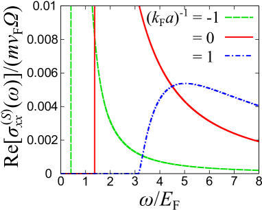
Figure 2: Spectra of the optical spin conductivity in a spin-1/2 superfluid Fermi gas at zero temperature. The conductivities vanish for small $\omega$ due to the spin-singlet pairing. At $(k_{\rm F}a)^{-1}=-1,0$, positive chemical potentials result in coherence peaks near the thresholds. Here, $v_{\rm F}=k_{\rm F}/m$ is the Fermi velocity and $\Omega$ is the volume.

Equation (6) clarifies that the structure of the quasiparticle spectrum strongly affects $\mathrm{Re}\,\sigma_{xx}^{(S)}(\omega)$. It is notable that $\mathrm{Re}\,\sigma_{xx}^{(S)}(\omega)$ vanishes for $|\omega|<2E_{\mathrm{gap}}$ as shown by $\theta(|\omega|-2E_{\mathrm{gap}})$ in Eq. (III). This reflects the fact that spin excitations are associated with the dissociation of spin-singlet Cooper pairs or molecules and require energy being larger than $2E_{\mathrm{gap}}$. Figure 2 shows the spectra of the optical spin conductivity for different interaction strengths. The behavior of $\mathrm{Re}\,\sigma_{xx}^{(S)}(\omega)$ near the threshold ($|\omega|\to 2E_{\mathrm{gap}}+0$) depends on the sign of the chemical potential Note:mu :

$$\mathrm{Re}\,\sigma_{xx}^{(S)}(\omega)=\begin{cases}\frac{\Omega}{12\pi}\sqrt{\frac{m\mu^{3}}{2\Delta\delta\omega}}&(\mu>0)\\ \frac{\Delta^{2}\Omega}{48\pi}\sqrt{\frac{m\delta\omega^{3}}{\sqrt{\mu^{2}+\Delta^{2}}|\mu|^{5}}}&(\mu<0)\end{cases}$$ (8)

with $\delta\omega=|\omega|-2E_{\mathrm{gap}}\to+0$. In the case of $\mu>0$ [$(k_{\mathrm{F}}a)^{-1}=-1,0$ in Fig. 2], the flat band at $|{\bm{k}}|=\sqrt{2m\mu}$ results in the divergent behavior $\mathrm{Re}\,\sigma_{xx}^{(S)}(\omega)\sim 1/\sqrt{\delta\omega}$, which is the so-called coherence peak Schrieffer:1964 . On the other hand, $E_{{\bm{k}},{\rm F}}$ is a monotonically increasing function of $|{\bm{k}}|$ on the BEC side with $\mu<0$ [$(k_{\mathrm{F}}a)^{-1}=1$ in Fig. 2] and the optical spin conductivity decreases as $\mathrm{Re}\,\sigma_{xx}^{(S)}(\omega)\sim(\delta\omega)^{3/2}$. In this way, the optical spin conductivity proves the excitation properties and the aspects of a spin insulator in the superfluid Fermi gas. We emphasize that these transport properties of the superfluid cannot be captured by the conventional Drude conductivity, whose real part takes a Lorentz distribution.

We mention the validity of the mean-field analysis. For any $(k_{\mathrm{F}}a)^{-1}$, our result in Eq. (6) satisfies exact relations such as the $f$-sum rule in Eq. (4) and the high-frequency tail $\mathrm{Re}\,\sigma_{xx}^{(S)}(\omega)=C\Omega/[12\pi(m|\omega|)^{3/2}]$ Enss:2012 ; Note:S=1/2 ; Hofmann:2011 with Tan’s contact $C$ Tan:2008 . Indeed, the high-frequency asymptotics of Eq. III provides the mean-field value of the contact $C=m^{2}\Delta^{2}$. In addition, the mean-field theory employed in this paper gives semi-quantitative descriptions of physical quantities throughout the BCS-BEC crossover at zero temperature regardless of the presence of the strong interaction Horikoshi ; Note:mean-field .

IV Spin-1 polar condensate

The optical spin conductivity can also be useful for bosonic systems. To see this, we next investigate spin transport for a spin-1 BEC within the Bogoliubov theory kawaguchi ; Note:Bogoliubov . Focusing on the polar phase realized with ²³Na and ⁸⁷Rb Stamper-Kurn:2013 , we will show a nontrivial AC spin response, which is again different from the Drude conductivity. In this phase, bosons condense only in the $s_{z}=0$ channel, which is decoupled from the spin channels ($s_{z}=\pm 1$) Uchino:2010 . By definition of $\bm{J}_{S}(t)$, only quasiparticles in the spin channels contribute to spin transport and the $f$ sum of $\mathrm{Re}\,\sigma_{xx}^{(S)}(\omega)$ in Eq. (4) is related to the particle number $N_{1}+N_{-1}$ in the spin channels arising from quantum depletion Uchino:2010 .

The grand canonical Hamiltonian of the system is given by Uchino:2010

$$K =\sum_{\bm{k}}\sum_{s_{z}=0,\pm 1}(\varepsilon_{\bm{k}}+qs_{z}^{2}-\mu)a_{{\bm{k}},s_{z}}^{\dagger}a_{{\bm{k}},s_{z}}$$ (9)

$$\quad+\frac{c_{0}}{2\Omega}\sum_{{\bm{k}},{\bm{p}},{\bm{p}}^{\prime}}\sum_{s_{z},s_{z}^{\prime}}a_{{\bm{k}}/2+{\bm{p}},s_{z}}^{\dagger}a_{{\bm{k}}/2-{\bm{p}},s_{z}^{\prime}}^{\dagger}a_{{\bm{k}}/2-{\bm{p}}^{\prime},s_{z}}a_{{\bm{k}}/2+{\bm{p}}^{\prime},s_{z}^{\prime}}$$ (10)

$$\quad+\frac{c_{1}}{2\Omega}\sum_{{\bm{k}},{\bm{p}},{\bm{p}}^{\prime}}\sum_{s_{z},s_{z}^{\prime},s_{z}^{\prime\prime},s_{z}^{\prime\prime\prime}}\mathbf{S}_{s_{z},s_{z}^{\prime}}\cdot\mathbf{S}_{s_{z}^{\prime\prime},s_{z}^{\prime\prime\prime}}$$ (11)

$$\quad\times\,a_{{\bm{k}}/2+{\bm{p}},s_{z}}^{\dagger}a_{{\bm{k}}/2-{\bm{p}},s_{z}^{\prime\prime}}^{\dagger}a_{{\bm{k}}/2-{\bm{p}}^{\prime},s_{z}^{\prime}}a_{{\bm{k}}/2+{\bm{p}}^{\prime},s_{z}^{\prime\prime\prime}},$$ (12)

where $q$ characterizes the quadratic Zeeman effect Stamper-Kurn:2013 , $\mu$ is the chemical potential, $a_{{\bm{k}},s_{z}}$ is the annihilation operator of a Bose atom with spin $s_{z}$, and $\Omega$ is the volume of the system. In a spin-1 BEC, the interatomic interactions can be characterized by the spin-independent coupling constant $c_{0}>0$ and spin-dependent coupling constant $c_{1}$ Ho:1998 ; Ohmi:1998 . The spin-1 matrices $\mathbf{S}_{s_{z},s_{z}^{\prime}}=(\mathrm{S}^{x}_{s_{z},s_{z}^{\prime}},\mathrm{S}^{y}_{s_{z},s_{z}^{\prime}},\mathrm{S}^{z}_{s_{z},s_{z}^{\prime}})$ are given by

$$\mathrm{S}^{x} =\frac{1}{\sqrt{2}}\begin{pmatrix}0&1&0\\ 1&0&1\\ 0&1&0\end{pmatrix},\ \mathrm{S}^{y}=\frac{i}{\sqrt{2}}\begin{pmatrix}0&-1&0\\ 1&0&-1\\ 0&1&0\end{pmatrix},$$ (13)

$$\mathrm{S}^{z} =\begin{pmatrix}1&0&0\\ 0&0&0\\ 0&0&-1\end{pmatrix}.$$ (14)

The optical spin conductivity within the Bogoliubov theory can be analytically evaluated. The spin current operator appearing in $\chi_{\alpha\beta}(\omega)$ is given by $\bm{J}_{S}=\sum_{\bm{k}}\frac{{\bm{k}}}{m}(a_{{\bm{k}},1}^{\dagger}a_{{\bm{k}},1}-a_{{\bm{k}},-1}^{\dagger}a_{{\bm{k}},-1})$. From the rotational symmetry of the system, $\sigma_{\alpha\alpha}^{(S)}(\omega)$ is independent of $\alpha=x,y,z$ and found to be (see Appendix C for details)

$$\mathrm{Re}\,\sigma_{xx}^{(S)}(\omega)=\sum_{\bm{k}}\frac{4\pi n_{0}^{2}c_{1}^{2}k_{x}^{2}}{m^{2}|\omega|^{3}}\delta(|\omega|-2E_{\bm{k},s}),$$ (15)

where $E_{\bm{k},s}=\sqrt{(\varepsilon_{\bm{k}}+q)(\varepsilon_{\bm{k}}+q+2n_{0}c_{1})}$ is the quasiparticle energy in the spin channels and $n_{0}$ is the condensate fraction. In the polar phase satisfying $q+n_{0}c_{1}>n_{0}|c_{1}|$, the spin excitations are gapped with the spin gap $E_{\mathrm{gap}}=\sqrt{q(q+2n_{0}c_{1})}$, while the gap is closed on boundaries of the phase ($q+n_{0}c_{1}=n_{0}|c_{1}|$). From Eq. (15), the optical spin conductivity is sensitive to whether spin excitations are gapped or gapless. By performing the integration over ${\bm{k}}$ in Eq. (15), the analytical form of $\mathrm{Re}\,\sigma_{xx}^{(S)}(\omega)$ is found to be

$$\mathrm{Re}\,\sigma_{xx}^{(S)}(\omega)=\frac{\sqrt{m}n_{0}^{2}c_{1}^{2}\Omega}{3\pi}\frac{[\varepsilon_{s}(\omega)]^{\frac{3}{2}}}{\omega^{2}\sqrt{\omega^{2}+4n_{0}^{2}c_{1}^{2}}}\theta(|\omega|-2E_{\mathrm{gap}})$$ (16)

with $\varepsilon_{s}(\omega)\equiv\sqrt{\omega^{2}+4n_{0}^{2}c_{1}^{2}}-2(q+n_{0}c_{1})$.

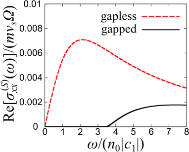
Figure 3: Optical spin conductivity spectra in a spin-1 BEC at zero temperature. The solid line shows the result in the spin-gapped case ($q=n_{0}c_{1}$), where the conductivity becomes nonzero for $\omega>2E_{\mathrm{gap}}$, while the dashed line shows that in the gapless case ($q+n_{0}c_{1}=n_{0}|c_{1}|$). Note that $v_{s}=\sqrt{n_{0}|c_{1}|/m}$ is associated with spin excitations and different from the sound velocity.

Figure 3 shows $\mathrm{Re}\,\sigma_{xx}^{(S)}(\omega)$ of the polar BEC. Inside the polar phase with the spin gap, $\mathrm{Re}\,\sigma_{xx}^{(S)}(\omega)$ vanishes for $|\omega|<2E_{\mathrm{gap}}$ and its decreasing behavior near the threshold ($|\omega|\to 2E_{\mathrm{gap}}+0$) is similar to that of the superfluid Fermi gas on the BEC side because of the similarity between $E_{\bm{k},s}$ and $E_{{\bm{k}},{\rm F}}$. On the other hand, $\mathrm{Re}\,\sigma_{xx}^{(S)}(\omega)$ on the phase boundaries with gapless spin excitations behaves linearly $\mathrm{Re}\,\sigma_{xx}^{(S)}(\omega)/\Omega=|\omega|/(48\pi v_{s})$ in the low-frequency region ($|\omega|\ll n_{0}|c_{1}|$) with the spin velocity $v_{s}=\sqrt{n_{0}|c_{1}|/m}$ (see Fig. 3). We note that this linear behavior is quite different from that of the Drude conductivity for conventional spin-gapless systems. In addition, by taking $\omega\to\pm\infty$ in Eq.(16), one can find the power-law tail $\mathrm{Re}\,\sigma_{xx}^{(S)}(\omega)=\sqrt{m}n_{0}^{2}c_{1}^{2}\Omega/(3\pi|\omega|^{3/2})$ in a similar way as for the superfluid Fermi gas. In this way, the obtained optical spin conductivity reflects the properties of spin excitations inherent to the polar BEC.

V Tomonaga-Luttinger liquids

In the case of the charge response, the optical conductivity is known to be a powerful tool for characterization of non-Fermi liquids where there is no well-defined quasiparticle sachdev ; chowdhury . To demonstrate the usefulness of the spin counterpart, here we consider one-dimensional quantum critical states with spin-1/2 where TL liquids being typical non-Fermi liquids are realized. In such states, the low-energy properties can be explained by an effective Hamiltonian where charge and spin degrees of freedom are separated, and therefore information of the spin part is expected to be captured by spin transport.

The effective Hamiltonian $H=H_{C}+H_{S}$ of TL liquids is bosonized as giamarchi

$$H_{C} =\frac{1}{2\pi}\int dx\,u_{C}[K_{C}(\pi\Pi_{C}(x))^{2}+(\nabla\phi_{C}(x))^{2}/K_{C}],$$ (17a)

$$H_{S} =\frac{1}{2\pi}\int dx\,u_{S}[K_{S}(\pi\Pi_{S}(x))^{2}+(\nabla\phi_{S}(x))^{2}/K_{S}]$$

$$\quad+\frac{2g}{(2\pi\alpha)^{2}}\int dx\,\cos(\sqrt{8}\phi_{S}(x)).$$ (17b)

Here, $H_{C(S)}$ is the Hamiltonian of the charge (spin) degree of freedom that consists of bosonic fields $\Pi_{C(S)}$ and $\phi_{C(S)}$ satisfying the canonical commutation relation:

$$[\phi_{C(S)}(x_{1}),\Pi_{C(S)}(x_{2})]=i\delta(x_{1}-x_{2}).$$ (18)

Physically, $\phi_{C(S)}$ and $\Pi_{C(S)}$ describe the charge (spin) density fluctuations and their conjugate phase fluctuations, respectively. In addition, $u_{C(S)}$ and $K_{C(S)}$ represent the velocity and the TL parameter in the charge (spin) component, respectively, $g$ is the coupling constant arising from the back-scattering process, and $\alpha$ is the cutoff of the low-energy theory Note:TLL . We note that the above Hamiltonian covers low-energy behaviors of experimentally important systems such as the Fermi-Hubbard model and Yang-Gaudin model.

To extract the essential feature, we perform bosonization allowing to express the spin current operator as $\sqrt{2}u_{S}K_{S}\Pi_{S}(x)$. In addition, $\cos(\sqrt{8}\phi_{S}(x))$ in $H_{C}$ does not commute with the spin current operator and generates nontrivial conductivity spectra. The basic feature of the spin conductivity is calculated with the memory function method giamarchi1991 ; giamarchi1992 (see Appendix D for details). At zero temperature, this leads to

$$\mathrm{Re}\,\sigma^{(S)}(\omega)\propto\omega^{4K_{S}-5}.$$ (19)

Thus, we find that the optical spin response is powerful in that $K_{S}$ essential to the critical properties yet elusive in cold atoms is determined by the frequency dependence. We also note that the similar power law dependence in the spin conductivity shows up for a spin insulating system where the back scattering process is relevant. In this case, the spin conductivity spectrum vanishes at frequencies below the spin gap yet obeys the power-law behavior at frequencies above the gap giamarchi .

VI Experimental realization

We now discuss how to measure $\sigma_{\alpha\beta}^{(S)}(\omega)$ in experiments. For ultracold atomic gases, we have several ways to induce the perturbation in Eq. (1). The most straightforward way is to apply a time-dependent gradient of a magnetic field $B({\bm{r}},t)\propto f_{\beta}(t)r_{\beta}$ along the $z$ axis medley ; Jotzu:2015 . Such a gradient potential can also be produced by the optical Stern-Gerlach effect Taie:2010 . Furthermore, ultracold atoms allow us to directly observe $\langle\bm{J}_{S}(t)\rangle=\frac{d\langle{\bm{X}}_{S}(t)\rangle}{dt}$ because

$$\langle{\bm{X}}_{S}(t)\rangle\equiv\int d{\bm{r}}\,{\bm{r}}\langle S_{z}({\bm{r}},t)\rangle$$ (20)

is given in terms of the observable spin density $\langle S_{z}({\bm{r}},t)\rangle$ medley ; valtolina . Hereafter, we focus on $\langle{\bm{X}}_{S}(t)\rangle$ rather than $\langle{\bm{J}}_{S}(t)\rangle$ to measure $\sigma_{\alpha\beta}^{(S)}(\omega)$.

In order to provide a concrete scheme of measurement, we consider a case with a single-frequency driving $f_{\beta}(t)=F_{\beta}\cos(\omega_{0}t)$. In this case, $\langle X_{S,\alpha}(t)\rangle$ shows an oscillating behavior, which is exactly related to $\sigma_{\alpha\beta}^{(S)}(\omega=\omega_{0})$ by

$$\frac{\langle\delta X_{S,\alpha}(t)\rangle}{F_{\beta}}$$

$$=-\frac{\mathrm{Im}\,\sigma_{\alpha\beta}^{(S)}(\omega_{0})}{\omega_{0}}\cos(\omega_{0}t)+\frac{\mathrm{Re}\,\sigma_{\alpha\beta}^{(S)}(\omega_{0})}{\omega_{0}}\sin(\omega_{0}t)$$ (21)

with $\langle\delta X_{S,\alpha}(t)\rangle\equiv\langle X_{S,\alpha}(t)\rangle-\langle X_{S,\alpha}\rangle_{0}$ (see Appendix E for details). Thus, $\sigma_{\alpha\beta}^{(S)}(\omega_{0})$ can be extracted through the oscillation analysis of $\langle X_{S,\alpha}(t)\rangle$ Note:Measurement_proposals . We next discuss feasibility in realistic experiments. An accessible region of $\omega_{0}$ depends on the way to generate $f_{\beta}(t)$. For a magnetic-field gradient, it is feasible up to frequencies of the order of kHz while noises coming from back electromotive forces to coils and metallic chambers would become significant in higher $\omega_{0}$ Nakajima:private_communications . On the other hand, a higher frequency region can easily be accessed by an optical driving force. There, the lower bound of $\omega_{0}$ would be determined so as to avoid heating coming from photon scatterings Nakajima:private_communications . In the case of the spin-1/2 Fermi superfluid, a typical many-body scales such as $\Delta$ is about $1$kHz, which can be accessible with both magnetic and optical gradients (see e.g. Ref. Biss:2022 and references therein). In addition, noises to the magnitude of $\sigma_{\alpha\beta}^{(S)}(\omega)$ would arise from measurement of $\langle S_{z}({\bm{r}},t)\rangle$ and the accuracy of $F_{\alpha}$ in each cycle.

VII Extensions of the results and proposed method

We now discuss generalizations of our results [Eqs. (3) and (4)] and proposal to measure $\sigma_{\alpha\beta}^{(S)}(\omega)$ based on Eq. (VI). First, we point out that Eqs. (3) and (4) as well as the measurement scheme for $S=1/2$ is naturally extended to two-component bosons Myatt:1996 ; Hall:1998a ; Hall:1998b by regarding two species as spin-up and spin-down states.

We next discuss an extension of the driving force to measure $\sigma_{\alpha\beta}^{(S)}(\omega)$. While generation of a pure spin current was considered so far, a more general time-dependent potential gradient inducing both mass and spin currents may be more practical in some experimental setups. For example, such a perturbation has been realized by applying a magnetic-field gradient to ⁴⁰K atoms with two hyperfine states Jotzu:2015 . We find that this kind of perturbation is also available to measure $\sigma_{\alpha\beta}^{(S)}(\omega)$ when investigating spin-1/2 gases confined by harmonic or box traps (see Appendix F for details). In particular, in the spin-balanced case, cross correlations between mass and spin vanish, so that Eq. (VI) holds even when both mass and spin currents are induced. The extension of our measurement scheme to spin-imbalanced cases is also possible.

Our results can also be generalized to spin-orbit coupled systems without spin conservation. Spin transport in these systems has been actively studied not only in spintronics sinova but also in cold-atom experiments galitski ; Li:2019 ; spielman . Even in such systems, $\sigma_{\alpha\beta}^{(S)}(\omega)$ satisfying Eqs. (3) and (4) can be defined and measured by simply generalizing our proposed method. To see this, we consider two-component gases with spin-orbit and Rabi couplings realized with ultracold atoms Lin:2011 ; Wang:2012 ; Cheuk:2012 (see Appendix G for details). For convenience, we define $X_{S,\alpha}^{\hat{a}}\equiv\int d{\bm{r}}\,r_{\alpha}S_{\hat{a}}({\bm{r}})$ and $\delta H_{\beta}^{\hat{b}}(t)\equiv-f_{\beta}^{\hat{b}}(t)X_{S,\beta}^{\hat{b}}$, where $S_{\hat{a}}({\bm{r}})$ is the spin density operator along the direction $\hat{a}=x,y,z$ in spin space. We emphasize that $\langle X_{S,\alpha}^{\hat{a}}(t)\rangle$ can be measured by observing the spin density. In the spin-conserved case, Eq. (VI) relates $\sigma_{\alpha\beta}^{(S)}(\omega)$ to the oscillating $\langle X_{S,\alpha}^{z}(t)\rangle$ under the perturbation $\delta H_{\beta}^{z}(t)$ [Eq. (1)]. In the presence of the spin-orbit and Rabi couplings, $\sigma_{\alpha\beta}^{(S)}(\omega)$ is rewritten in terms of the thermal average of $S_{x}({\bm{r}})$ and four responses of $\langle X_{S,\alpha}^{\hat{a}}(t)\rangle$ under $\delta H_{\beta}^{\hat{b}}(t)$ with $\hat{a},\hat{b}\in\{y,z\}$ [see Eq. (G)]. These responses can be measured from oscillation analyses similar to Eq. (VI).

Finally, as in the charge response Shimizu:2010 , Eqs. (3) and (4) can be generalized to nonequilibrium systems with spin conservation, whose optical spin conductivity is measurable from spin dynamics in cold-atom experiments (see Appendix H for details). Unlike in equilibrium, the nonequilibrium spin conductivity can have a negative real part associated with energy gain Tsuji:2009 .

VIII Other promising applications

The optical spin conductivity has a variety of prospects. The potential of $\sigma_{\alpha\beta}^{(S)}(\omega)$ to detect a topological phase transition has been recently pointed out Tajima:2021 . Our formalism and proposal are applicable to optical lattice systems. For instance, it is important to confirm an anomalous frequency dependence in $\sigma^{(S)}(\omega)$ of spin chains Agrawal:2020 whose spin superdiffusion has attracted attention Bulchandani:2021 ; Wei:2021 . As the optical charge conductivity measurement has already served as valuable probes for pseudogap phenomena Homes:1993 , non-Fermi liquids chowdhury ; sachdev , and photoinduced insulator-metal transitions Iwai:2003 ; Cavalleri:2004 ; Okamoto:2007 , $\sigma_{\alpha\beta}^{(S)}(\omega)$ is expected to be a key quantity to understand spin dynamics of strongly correlated and nonequilibrium systems. For instance, unlike photoemission spectroscopy conventionally used to study pseudogaps of ultracold atoms Stewart:2008 ; Gaebler:2010 ; Sagi:2015 , $\sigma_{\alpha\beta}^{(S)}(\omega)$ involves both upper and lower branches of single-particle excitations, so that measurement of $\sigma_{\alpha\beta}^{(S)}(\omega)$ would deepen our understanding of the pseudogap phenomenon Mueller:2017 . In terms of unconventional quantum liquids, it is also interesting to investigate a spin liquid Savary:2016 , which has recently been realized with cold atoms Semeghini:2021 . Finally, applications to nonequilibrium states such as Floquet time crystals Else:2016 and nonlinear responses such as shift spin currents morimoto are also promising routes for the spin conductivity.

IX Conclusion

In this paper, we discussed the optical spin conductivity $\sigma_{\alpha\beta}^{(S)}(\omega)$, which serves as a valuable probe to examine many-body interacting systems with spin degrees of freedom and can be measured with existing methods in cold-atom experiments. First, the formalism of $\sigma_{\alpha\beta}^{(S)}(\omega)$ applicable to both continuum and optical lattice systems was provided. We then theoretically investigated three systems to show the availability of the optical spin conductivity. For the superfluid Fermi gas, the gapped single-particle excitations result in the gap of the spectrum $\mathrm{Re}\,\sigma_{xx}^{(S)}(\omega)$ and the flat band for $\mu>0$ leads to the coherence peak. For the spinor BEC, $\mathrm{Re}\,\sigma_{xx}^{(S)}(\omega)$ detects gapped spin excitations in the polar phase as well as gapless spin excitations on the phase boundaries, and its $f$ sum is related to quantum depletion. In addition, from Eq. (19), the optical spin conductivity is found to be related to the spin part of the TL liquid parameter $K_{S}$ elusive in cold-atom experiments. We also proposed that the optical spin conductivity can be measured from the oscillation in spin dynamics [Eq. (VI)]. This proposal can be extended to various cases including spin-orbit coupled and nonequilibrium systems. As mentioned in Sec. VIII, various applications of the optical spin conductivity as probes for exotic spin dynamics are promising.

Note added— When this paper was being finalized, there appeared a paper Carlini:2021 , where a spin drag effect and related $f$-sum rules due to a spin-dependent perturbation are discussed.

Appendix A Formalism with spin conservation

We consider spin transport in a system with spin $S=1/2,1,3/2,\cdots$. Here, we employ the first quantization formalism to clarify the connection between the spin current and the spin-resolved center-of-mass motion. The Hamiltonian of the system is given by $\mathcal{H}(t)=H+\delta H_{\beta}(t)$. The nonperturbative term $H$ is given by

$$H=\sum_{(s_{z},i)}\left(\frac{1}{2m}\left[{\bm{p}}_{s_{z},i}-{\bm{A}}_{s_{z}}({\bm{r}}_{s_{z},i})\right]^{2}+V_{s_{z}}({\bm{r}}_{s_{z},i})\right)+H_{\rm int},$$ (22)

where $m$ is a mass of a particle and labels of particles take $s_{z}=-S,-S+1,\cdots,S$ and $i=1,2,\cdots,N_{s_{z}}$ with $N_{s_{z}}$ being the particle number in the $s_{z}$ component. The operators ${\bm{r}}_{s_{z},i}$ and ${\bm{p}}_{s_{z},i}$ denote the coordinate and momentum operators of the particle with a label $(s_{z},i)$ and they satisfy the following canonical commutation relations:

$$[(r_{s_{z},i})_{\alpha},(r_{s_{z}^{\prime},i^{\prime}})_{\beta}] =[(p_{s_{z},i})_{\alpha},(p_{s_{z}^{\prime},i^{\prime}})_{\beta}]=0,$$ (23a)

$$[(r_{s_{z},i})_{\alpha},(p_{s_{z}^{\prime},i^{\prime}})_{\beta}] =i\delta_{s_{z}s_{z}^{\prime}}\delta_{ii^{\prime}}\delta_{\alpha\beta},$$ (23b)

where $\alpha$ and $\beta$ denote Cartesian components $x,y,z$ in the coordinate space. The functions ${\bm{A}}_{s_{z}}({\bm{r}})$ and $V_{s_{z}}({\bm{r}})$ are spin-dependent vector and scalar potentials, respectively, and the interaction term $H_{\rm int}$ is assumed to be described by pairwise potentials and commute with the $z$ component of the spin density operator $S_{z}({\bm{r}})=\sum_{(s_{z},i)}s_{z}\delta({\bm{r}}-{\bm{r}}_{s_{z},i})$. The time-dependent perturbation term is given by

$$\delta H_{\beta}(t)=-\int d{\bm{r}}\,f_{\beta}(t)r_{\beta}S_{z}({\bm{r}})=-f_{\beta}(t)X_{S,\beta},$$ (24)

where $f_{\beta}(t)$ provides a driving force in the direction $\beta$ coupled to the spin density $S_{z}({\bm{r}})$. The operator ${\bm{X}}_{S}\equiv\int d{\bm{r}}\,{\bm{r}}S_{z}({\bm{r}})$ measures the coordinate characterizing spin dynamics driven by $f_{\beta}(t)$. In terms of the spin-resolved center-of-mass coordinate $\bm{R}_{s_{z}}=\sum_{i=1}^{N_{s_{z}}}{\bm{r}}_{s_{z},i}/N_{s_{z}}$, ${\bm{X}}_{S}$ is rewritten as ${\bm{X}}_{S}=\sum_{s_{z}}s_{z}N_{s_{z}}{\bm{R}}_{s_{z}}$. The perturbation generates a spin current, whose corresponding operator in the Heisenberg picture is given by $\bm{J}_{S}(t)=\sum_{(s_{z},i)}s_{z}\frac{d{\bm{r}}_{s_{z},i}(t)}{dt}$. This operator can be rewritten as

$$\bm{J}_{S}(t)=\frac{d{\bm{X}}_{S}(t)}{dt}=\sum_{(s_{z},i)}\frac{s_{z}}{m}[{\bm{p}}_{s_{z},i}(t)-{\bm{A}}_{s_{z}}({\bm{r}}_{s_{z},i}(t))].$$ (25)

A.1 Optical spin conductivity

We now derive the expression of the optical spin conductivity $\sigma_{\alpha\beta}^{(S)}(\omega)$ [Eq. (3)] in terms of a retarded response function for a spin current. The optical spin conductivity $\sigma_{\alpha\beta}^{(S)}(\omega)$ is given as the linear response of the spin current to the driving force:

$$\langle\tilde{J}_{S,\alpha}(\omega)\rangle=\sigma_{\alpha\beta}^{(S)}(\omega)\tilde{f}_{\beta}(\omega),$$ (26)

where $\tilde{J}_{S,\alpha}(\omega)$ and $\tilde{f}_{\alpha}(\omega)$ are the Fourier transforms of $J_{S,\alpha}(t)$ and $f_{\alpha}(t)$, respectively, and $\langle\cdots\rangle$ denotes the expectation value with respect to a nonequilibrium state driven by the external force. The Kubo formula provides

$$\sigma_{\alpha\beta}^{(S)}(\omega)=i\int_{-\infty}^{\infty}\!\!dt\,e^{i\omega^{+}t}\theta(t)\langle[J_{S,\alpha}(t),X_{S,\beta}(0)]\rangle_{0},$$ (27)

where $\omega^{+}\equiv\omega+i0^{+}$, $\theta(t)$ is the Heaviside step function, and $\langle\cdots\rangle_{0}$ denotes the thermal average without the external force. From Eq. (25) and $\langle[J_{S,\alpha}(t),X_{S,\beta}(0)]\rangle_{0}=\langle[J_{S,\alpha}(0),X_{S,\beta}(-t)]\rangle_{0}$ resulting from time translation invariance, performing the integration by parts yields

$$\sigma_{\alpha\beta}^{(S)}(\omega)=-\frac{1}{\omega^{+}}\langle[J_{S,\alpha}(0),X_{S,\beta}(0)]\rangle_{0}+\frac{i}{\omega^{+}}\chi_{\alpha\beta}(\omega),$$ (28)

where

$$\chi_{\alpha\beta}(\omega)=-i\int_{-\infty}^{\infty}\!\!dt\,e^{i\omega^{+}t}\theta(t)\langle[J_{S,\alpha}(t),J_{S,\beta}(0)]\rangle_{0}$$ (29)

is the retarded response function for the spin current. Using Eqs. (23) and (25), we obtain

$$[J_{S,\alpha}(0),X_{S,\beta}(0)]=-i\delta_{\alpha\beta}\sum_{s_{z}}\frac{s_{z}^{2}N_{s_{z}}}{m}.$$ (30)

Substituting this into Eq. (28), we finally find Eq. (3):

$$\sigma_{\alpha\beta}^{(S)}(\omega)=\frac{i}{\omega^{+}}\left(\delta_{\alpha\beta}\sum_{s_{z}}\frac{s_{z}^{2}N_{s_{z}}}{m}+\chi_{\alpha\beta}(\omega)\right).$$ (31)

We next turn to the $f$-sum rule [Eq. (4)], which is the exact constraint on the integral of $\sigma_{\alpha\beta}^{(S)}(\omega)$ over $\omega$. The causality condition in the retarded function $\chi_{\alpha\beta}(\omega)$ leads to the Kramers-Kronig relation:

$$\mathrm{Re}\,\chi_{\alpha\beta}(\omega)=\mathcal{P}\int_{-\infty}^{\infty}\frac{d\omega^{\prime}}{\pi}\frac{\mathrm{Im}\,\chi_{\alpha\beta}(\omega^{\prime})}{\omega^{\prime}-\omega},$$ (32)

where $\mathcal{P}$ denotes the Cauchy principal value. Using this relation, we can obtain the $f$-sum rule [Eq. (4)]:

$$\int_{-\infty}^{\infty}\!\!\frac{d\omega}{\pi}\mathrm{Re}\,\sigma_{\alpha\beta}^{(S)}(\omega)=\delta_{\alpha\beta}\sum_{s_{z}}\frac{s_{z}^{2}N_{s_{z}}}{m}.$$ (33)

Appendix B Spin-1/2 superfluid Fermi gas

Here we compute the optical spin conductivity for a spin-1/2 Fermi superfluid at zero temperature within the BCS-Leggett mean-field theory Eagles:1969 ; Leggett:1980 . In the mean-field theory, Eq. (III) reduces to

$$K_{\mathrm{BCS}}=E_{\mathrm{GS}}+\sum_{{\bm{k}},\sigma}E_{{\bm{k}},{\rm F}}\gamma_{{\bm{k}},\sigma}^{\dagger}\gamma_{{\bm{k}},\sigma},$$ (34)

where $E_{{\bm{k}},{\rm F}}=\sqrt{(\varepsilon_{\bm{k}}-\mu)^{2}+\Delta^{2}}$ is the quasiparticle energy with the superfluid order parameter $\Delta$. Since the ground state energy $E_{\mathrm{GS}}$ does not contribute to spin transport, we do not provide its explicit form. The creation and annihilation operators $\gamma_{{\bm{k}},\sigma}^{\dagger},\,\gamma_{{\bm{k}},\sigma}$ of quasiparticles are given by the Bogoliubov transformation:

$$\begin{pmatrix}\gamma_{{\bm{k}},\uparrow}^{\dagger}\\ \gamma_{-{\bm{k}},\downarrow}\end{pmatrix}=\begin{pmatrix}u_{{\bm{k}},{\rm F}}&-v_{{\bm{k}},{\rm F}}\\ v_{{\bm{k}},{\rm F}}&u_{{\bm{k}},{\rm F}}\end{pmatrix}\begin{pmatrix}c_{{\bm{k}},\uparrow}^{\dagger}\\ c_{-{\bm{k}},\downarrow}\end{pmatrix}$$ (35)

with

$$u_{{\bm{k}},{\rm F}}=\sqrt{\frac{1}{2}\left(1+\frac{\varepsilon_{\bm{k}}-\mu}{E_{{\bm{k}},{\rm F}}}\right)},\quad v_{{\bm{k}},{\rm F}}=\sqrt{\frac{1}{2}\left(1-\frac{\varepsilon_{\bm{k}}-\mu}{E_{{\bm{k}},{\rm F}}}\right)}.$$ (36)

The operators $\gamma_{{\bm{k}},\sigma}^{\dagger},\,\gamma_{{\bm{k}},\sigma}$ satisfy the following anticommutation relations:

$$\{\gamma_{{\bm{k}},\sigma},\gamma_{{\bm{k}}^{\prime},\sigma^{\prime}}\} =\{\gamma_{{\bm{k}},\sigma}^{\dagger},\gamma_{{\bm{k}}^{\prime},\sigma^{\prime}}^{\dagger}\}=0,$$ (37a)

$$\{\gamma_{{\bm{k}},\sigma},\gamma_{{\bm{k}}^{\prime},\sigma^{\prime}}^{\dagger}\} =\delta_{{\bm{k}}{\bm{k}}^{\prime}}\delta_{\sigma\sigma^{\prime}}.$$ (37b)

In the mean field approximation, $\Delta$ and $\mu$ for given $a$ and $N=N_{\uparrow}+N_{\downarrow}$ are determined by self-consistently solving the following gap and particle number equations:

$$-\frac{m}{4\pi a} =\frac{1}{\Omega}\sum_{\bm{k}}\left(\frac{1}{2E_{{\bm{k}},{\rm F}}}-\frac{1}{2\varepsilon_{\bm{k}}}\right),$$ (38)

$$N =\sum_{\bm{k}}\left(1-\frac{\varepsilon_{\bm{k}}-\mu}{E_{{\bm{k}},{\rm F}}}\right).$$ (39)

B.1 Current correlation function

Here, we calculate the correlation function $\chi_{\alpha\beta}(\omega)$ in Eq. (29) for the superfluid Fermi gas. In the second quantization formalism, $\bm{J}_{S}$ in Eq. (25) is rewritten as

$$\bm{J}_{S}=\sum_{\bm{k}}\frac{{\bm{k}}}{2m}(c_{{\bm{k}},\uparrow}^{\dagger}c_{{\bm{k}},\uparrow}-c_{{\bm{k}},\downarrow}^{\dagger}c_{{\bm{k}},\downarrow}).$$ (40)

Substituting the inverse of the Bogoliubov transformation in Eq. (35) into this yields

$$\bm{J}_{S} =\sum_{\bm{k}}\frac{{\bm{k}}}{2m}\left[(u_{{\bm{k}},{\rm F}}^{2}-v_{{\bm{k}},{\rm F}}^{2})(\gamma_{{\bm{k}},\uparrow}^{\dagger}\gamma_{{\bm{k}},\uparrow}+\gamma_{-{\bm{k}},\downarrow}^{\dagger}\gamma_{-{\bm{k}},\downarrow})\right.$$

$$\quad\left.+2v_{{\bm{k}},{\rm F}}^{2}+2u_{{\bm{k}},{\rm F}}v_{{\bm{k}},{\rm F}}(\gamma_{{\bm{k}},\uparrow}^{\dagger}\gamma_{-{\bm{k}},\downarrow}^{\dagger}+\gamma_{-{\bm{k}},\downarrow}\gamma_{{\bm{k}},\uparrow})\right].$$ (41)

In the Heisenberg picture, $\bm{J}_{S}(t)=U_{\mathrm{BCS}}^{\dagger}(t)\bm{J}_{S}U_{\mathrm{BCS}}(t)$ with $U_{\mathrm{BCS}}(t)=\exp(-iK_{\mathrm{BCS}}\,t)$ reads

$$\bm{J}_{S}(t) =\sum_{\bm{k}}\frac{{\bm{k}}}{2m}\Bigl{[}(u_{{\bm{k}},{\rm F}}^{2}-v_{{\bm{k}},{\rm F}}^{2})(\gamma_{{\bm{k}},\uparrow}^{\dagger}\gamma_{{\bm{k}},\uparrow}+\gamma_{-{\bm{k}},\downarrow}^{\dagger}\gamma_{-{\bm{k}},\downarrow})$$

$$\quad+2u_{{\bm{k}},{\rm F}}v_{{\bm{k}},{\rm F}}(e^{2iE_{{\bm{k}},{\rm F}}t}\gamma_{{\bm{k}},\uparrow}^{\dagger}\gamma_{-{\bm{k}},\downarrow}^{\dagger}+e^{-2iE_{{\bm{k}},{\rm F}}t}\gamma_{-{\bm{k}},\downarrow}\gamma_{{\bm{k}},\uparrow})$$

$$\quad+2v_{{\bm{k}},{\rm F}}^{2}\Bigr{]},$$ (42)

where $\gamma_{{\bm{k}},\sigma}(t)=U_{\mathrm{BCS}}^{\dagger}(t)\gamma_{{\bm{k}},\sigma}U_{\mathrm{BCS}}(t)=\gamma_{{\bm{k}},\sigma}e^{-iE_{{\bm{k}},{\rm F}}t}$ was used.

Let us now evaluate the correlation function in Eq. (29) at zero temperature. Using Eqs. (36), (37), and (B.1) as well as $\langle\gamma_{{\bm{k}},\sigma}^{\dagger}\gamma_{{\bm{k}},\sigma}\rangle_{0}=0$ at zero temperature, the expectation value in Eq. (29) is

$$\langle[J_{S,\alpha}(t),J_{S,\beta}(0)]\rangle_{0}=\sum_{{\bm{k}}}\frac{\Delta^{2}k_{\alpha}k_{\beta}}{4m^{2}E_{{\bm{k}},{\rm F}}^{2}}\left(e^{-2iE_{{\bm{k}},{\rm F}}t}-e^{2iE_{{\bm{k}},{\rm F}}t}\right).$$ (43)

Therefore, the correlation function for the superfluid Fermi gas is found to be

$$\chi_{\alpha\beta}(\omega)=\delta_{\alpha\beta}\sum_{\bm{k}}\frac{\Delta^{2}k_{\alpha}^{2}}{4m^{2}E_{{\bm{k}},{\rm F}}^{2}}\left(\frac{1}{\omega^{+}-2E_{{\bm{k}},{\rm F}}}-\frac{1}{\omega^{+}+2E_{{\bm{k}},{\rm F}}}\right).$$ (44)

B.2 Spin conductivity

Let us evaluate the real part of the optical spin conductivity. Equation (3) provides

$$\mathrm{Re}\,\sigma_{xx}^{(S)}(\omega)=\mathcal{D}_{S}\delta(\omega)-\frac{1}{\omega}\mathrm{Im}\,\chi_{xx}(\omega),$$ (45)

where $\mathcal{D}_{S}=\pi\left[N/4m+\mathrm{Re}\,\chi_{xx}(0)\right]$ is the spin Drude weight. Using Eqs. (39) and (44), replacing $\sum_{\bm{k}}\to\Omega\int d^{3}{\bm{k}}/(2\pi)^{3}$, and performing the integration over $k=|{\bm{k}}|$ by parts, we can find $\mathcal{D}_{S}=0$ in this case. By substituting Eq. (44) into the second term in Eq. (45), the real part of $\sigma_{xx}^{(S)}(\omega)$ is given by

$$\mathrm{Re}\,\sigma_{xx}^{(S)}(\omega) =\sum_{\bm{k}}\frac{\pi\Delta^{2}k_{x}^{2}}{m^{2}|\omega|^{3}}\delta(|\omega|-2E_{{\bm{k}},{\rm F}}).$$ (46)

Using Eq. (39), we can straightforwardly confirm that this spin conductivity satisfies the $f$-sum rule in Eq. (4).

Appendix C Spin-1 polar Bose-Einstein condensate

Here we compute the optical spin conductivity for a spin-1 Bose-Einstein condensate (BEC) at zero temperature within the Bogoliubov theory kawaguchi . In the polar phase, the condensate is characterized by $\langle a_{{\bm{k}}=\mathbf{0},s_{z}}\rangle=\sqrt{n_{0}}\delta_{s_{z}0}$ with the condensate fraction $n_{0}$ and is stabilized in the plane of $(q,n_{0}c_{1})$ satisfying $q+n_{0}c_{1}>n_{0}|c_{1}|$. By using the Bogoliubov theory, where the effect of $a_{{\bm{k}}\neq\mathbf{0}}$ on $K$ [Eq. (9)] is incorporated up to quadratic order, $K$ reduces to Uchino:2010

$$K_{\mathrm{Bog}} =E_{\mathrm{GS}}+\sum_{{\bm{k}}\neq\mathbf{0}}\left[E_{{\bm{k}},d}\beta^{\dagger}_{{\bm{k}},d}\beta_{{\bm{k}},d}\right.$$ (47)

$$\quad\left.+E_{{\bm{k}},s}(\beta^{\dagger}_{{\bm{k}},s_{x}}\beta_{{\bm{k}},s_{x}}+\beta^{\dagger}_{{\bm{k}},s_{y}}\beta_{{\bm{k}},s_{y}})\right].$$ (48)

Since the ground-state energy $E_{\mathrm{GS}}$ does not contribute to spin transport as in the case of the spin-$1/2$ superfluid Fermi gas, we do not show its explicit form. The quasiparticle energies in the density ($d$) and spin ($s$) channels are given by $E_{{\bm{k}},d}=\sqrt{\varepsilon_{\bm{k}}(\varepsilon_{\bm{k}}+2n_{0}c_{0})}$ and $E_{{\bm{k}},s}=\sqrt{(\varepsilon_{\bm{k}}+q)(\varepsilon_{\bm{k}}+q+2n_{0}c_{1})}$, respectively. The operators $\beta_{{\bm{k}},d}$, $\beta_{{\bm{k}},s_{x}}$, and $\beta_{{\bm{k}},s_{y}}$ denote the annihilation operators of quasiparticles, which are related to

$$b_{{\bm{k}},d} =a_{{\bm{k}},0},$$ (49a)

$$b_{{\bm{k}},s_{x}} =\frac{1}{\sqrt{2}}(a_{{\bm{k}},1}+a_{{\bm{k}},-1}),$$ (49b)

$$b_{{\bm{k}},s_{y}} =\frac{i}{\sqrt{2}}(a_{{\bm{k}},1}-a_{{\bm{k}},-1})$$ (49c)

by the Bogoliubov transformations:

$$b_{{\bm{k}},d} =u_{{\bm{k}},d}\beta_{{\bm{k}},d}-v_{{\bm{k}},d}\beta^{\dagger}_{-{\bm{k}},d},$$ (50a)

$$b_{{\bm{k}},s_{x}} =u_{{\bm{k}},s}\beta_{{\bm{k}},s_{x}}-v_{{\bm{k}},s}\beta^{\dagger}_{-{\bm{k}},s_{x}},$$ (50b)

$$b_{{\bm{k}},s_{y}} =u_{{\bm{k}},s}\beta_{{\bm{k}},s_{y}}-v_{{\bm{k}},s}\beta^{\dagger}_{-{\bm{k}},s_{y}}$$ (50c)

with

$$u_{{\bm{k}},d} =\sqrt{\frac{\varepsilon_{\bm{k}}+n_{0}c_{0}+E_{{\bm{k}},d}}{2E_{{\bm{k}},d}}},$$ (51a)

$$v_{{\bm{k}},d} =\sqrt{\frac{\varepsilon_{\bm{k}}+n_{0}c_{0}-E_{{\bm{k}},d}}{2E_{{\bm{k}},d}}},$$ (51b)

$$u_{{\bm{k}},s} =\sqrt{\frac{\varepsilon_{\bm{k}}+q+n_{0}c_{1}+E_{{\bm{k}},s}}{2E_{{\bm{k}},s}}},$$ (51c)

$$v_{{\bm{k}},s} =\sqrt{\frac{\varepsilon_{\bm{k}}+q+n_{0}c_{1}-E_{{\bm{k}},s}}{2E_{{\bm{k}},s}}}.$$ (51d)

Since the density channel does not contribute to spin transport, we below consider the spin channels. The annihilation and creation operators of quasiparticles in the spin channels satisfy the following commutation relations:

$$[\beta_{{\bm{k}},s_{j}},\beta_{{\bm{k}},s_{j^{\prime}}}] =[\beta_{{\bm{k}},s_{j}}^{\dagger},\beta_{{\bm{k}},s_{j^{\prime}}}^{\dagger}]=0,$$ (52a)

$$[\beta_{{\bm{k}},s_{j}},\beta_{{\bm{k}},s_{j^{\prime}}}^{\dagger}] =\delta_{{\bm{k}}{\bm{k}}^{\prime}}\delta_{s_{j}s_{j^{\prime}}}$$ (52b)

with $j,j^{\prime}\in\{x,y\}$.

C.1 Current correlation function

Here, we calculate the correlation function $\chi_{\alpha\beta}(\omega)$ in Eq. (29) for the spinor BEC in the polar phase. In the second quantization formalism, $\bm{J}_{S}$ in Eq. (25) is rewritten as

$$\bm{J}_{S} =\sum_{\bm{k}}\frac{{\bm{k}}}{m}(a_{{\bm{k}},1}^{\dagger}a_{{\bm{k}},1}-a_{{\bm{k}},-1}^{\dagger}a_{{\bm{k}},-1})$$ (53)

$$=-i\sum_{{\bm{k}}}\frac{{\bm{k}}}{m}(b^{\dagger}_{{\bm{k}},s_{x}}b_{{\bm{k}},s_{y}}-b^{\dagger}_{{\bm{k}},s_{y}}b_{{\bm{k}},s_{x}}),$$ (54)

where Eqs. (49) were used. Substituting Eqs. (50) into this and using Eqs. (52), we obtain

$$\bm{J}_{S} =-i\sum_{{\bm{k}}}\frac{{\bm{k}}}{m}\left[(u_{{\bm{k}},s}^{2}+v_{{\bm{k}},s}^{2})(\beta^{\dagger}_{{\bm{k}},s_{x}}\beta_{{\bm{k}},s_{y}}-\beta^{\dagger}_{{\bm{k}},s_{y}}\beta_{{\bm{k}},s_{x}})\right.$$

$$\quad\left.-2u_{{\bm{k}},s}v_{{\bm{k}},s}(\beta^{\dagger}_{{\bm{k}},s_{x}}\beta^{\dagger}_{-{\bm{k}},s_{y}}-\beta_{{\bm{k}},s_{x}}\beta_{-{\bm{k}},s_{y}})\right].$$ (55)

In the Heisenberg picture, $\bm{J}_{S}(t)=U_{\mathrm{Bog}}^{\dagger}(t)\bm{J}_{S}U_{\mathrm{Bog}}(t)$ with $U_{\mathrm{Bog}}(t)=\exp(-iK_{\mathrm{Bog}}\,t)$ reads

$$\bm{J}_{S}(t) =\sum_{{\bm{k}}}\frac{{\bm{k}}}{m}\left[-i(u_{{\bm{k}},s}^{2}+v_{{\bm{k}},s}^{2})\beta^{\dagger}_{{\bm{k}},s_{x}}\beta_{{\bm{k}},s_{y}}\right.$$

$$\quad\left.+2i\,u_{{\bm{k}},s}v_{{\bm{k}},s}e^{2iE_{{\bm{k}},s}t}\beta^{\dagger}_{{\bm{k}},s_{x}}\beta^{\dagger}_{-{\bm{k}},s_{y}}+\mathrm{h.c.}\right],$$ (56)

where $\beta_{{\bm{k}},s_{j}}(t)=U_{\mathrm{Bog}}^{\dagger}(t)\beta_{{\bm{k}},s_{j}}U_{\mathrm{Bog}}(t)=\beta_{{\bm{k}},s_{j}}e^{-iE_{{\bm{k}},s}t}$ was used.

Let us now evaluate the correlation function in Eq. (29) at zero temperature. Using Eqs. (51), (52), and (C.1) as well as $\langle\beta_{{\bm{k}},s_{j}}^{\dagger}\beta_{{\bm{k}},s_{j}}\rangle_{0}=0$ at zero temperature, the expectation value in Eq. (29) is

$$\langle[J_{S,\alpha}(t),J_{S,\beta}(0)]\rangle_{0}=\sum_{{\bm{k}}}\frac{n_{0}^{2}c_{1}^{2}k_{\alpha}k_{\beta}}{m^{2}E_{{\bm{k}},s}^{2}}\left(e^{-2iE_{{\bm{k}},s}t}-e^{2iE_{{\bm{k}},s}t}\right).$$ (57)

Therefore, the correlation function for the polar BEC is found to be

$$\chi_{\alpha\beta}(\omega)=\delta_{\alpha\beta}\sum_{\bm{k}}\frac{n_{0}^{2}c_{1}^{2}k_{\alpha}^{2}}{m^{2}E_{\bm{k},s}^{2}}\left(\frac{1}{\omega^{+}-2E_{\bm{k},s}}-\frac{1}{\omega^{+}+2E_{\bm{k},s}}\right).$$ (58)

C.2 Spin conductivity

Let us now evaluate the real part of the optical spin conductivity. The real part is given as the form of Eq. (45), where the spin Drude weight $\mathcal{D}_{S}=\pi\left[(N_{1}+N_{-1})/m+\mathrm{Re}\,\chi_{xx}(0)\right]$ in this case involves the quantum depletion $N_{1}+N_{-1}$ in the spin channels. Using $N_{1}+N_{-1}=\sum_{\bm{k}}2v_{{\bm{k}},s}^{2}$ Uchino:2010 and Eq. (58), we can see $\mathcal{D}_{S}=0$ in a similar way as for the superfluid Fermi gas. The real part thus reads

$$\mathrm{Re}\,\sigma_{xx}^{(S)}(\omega)=\sum_{\bm{k}}\frac{4\pi n_{0}^{2}c_{1}^{2}k_{x}^{2}}{m^{2}|\omega|^{3}}\delta(|\omega|-2E_{\bm{k},s}).$$ (59)

We can straightforwardly confirm that this spin conductivity satisfies the $f$-sum rule in Eq. (4). We note that the $f$ sum in this case is equivalent to the quantum depletion in the spin channel Uchino:2010 while that in the $S=1/2$ case provides the total particle number.

Appendix D Tomonaga-Luttinger liquid

Here we consider spin-1/2 one-dimensional quantum fluids where the low-energy description based on Tomonaga-Luttinger (TL) liquids is reasonable. In addition to the Hamiltonian $H=H_{C}+H_{S}$ [see Eqs. (17)], one can bosonize physical quantities in this case. For instance, the local current operator is expressed as

$$j_{C(S)}(x,t)=\sqrt{2}u_{C(S)}K_{C(S)}\Pi_{C(S)}(x,t).$$ (60)

Owing to the spin-charge separation and the formal similarity of the Hamiltonian between charge and spin sectors, as in the case of the charge conductivity giamarchi , one can obtain the spin conductivity expression as

$$\sigma^{(S)}(\omega)=\frac{i}{\omega}\left(\frac{2u_{S}K_{S}\Omega}{\pi}+\chi(\omega)\right),$$ (61)

where $\Omega$ is the one-dimensional volume and the retarded current-current correlation function $\chi(\omega)$ is given by Eq. (29) with $J_{S}(t)=\int dx\,j_{S}(x,t)$. In order to obtain the finite frequency dependence, we rewrite the conductivity as

$$\sigma^{(S)}(\omega)=\frac{2iu_{S}K_{S}\Omega}{\pi}\frac{1}{\omega+M(\omega)},$$ (62)

where $M(\omega)$ is called the memory function. One can perturbatively calculate $M(\omega)$, provided that $g$ is small. By performing the similar calculation with charge transport giamarchi1991 ; giamarchi1992 , we obtain

$$M(\omega) \approx\frac{g^{2}K_{S}}{\pi^{3}\alpha^{2}}\sin(2\pi K_{S})\Gamma^{2}(1-2K_{S})\frac{e^{-i\pi(2K_{S}-1)}}{\omega}$$

$$\quad\times\left(\frac{\alpha\omega}{2u_{S}}\right)^{4K_{S}-2},$$ (63)

where $\Gamma(z)$ is the gamma function and we assumed the zero temperature. For $K_{S}\geq 1$ that corresponds to cases of repulsive interactions, $\cos(\sqrt{8}\phi_{S})$ becomes irrelevant and therefore the TL liquid is realized. In this case, $M(\omega)$ is negligible compared with $\omega$ at low frequencies. Thus, by using Eq. (62), we find $\text{Re}[\sigma^{(S)}(\omega)]\sim\omega^{4K_{S}-5}$.

Appendix E Spin dynamics under single-frequency driving

Here, we derive Eq. (VI), which allows us to experimentally extract $\sigma_{\alpha\beta}^{(S)}(\omega)$ from spin dynamics driven by the perturbation [Eq. (1)]. We consider one of the simplest perturbations, i.e., the single-frequency driving $f_{\beta}(t)=F_{\beta}\cos(\omega_{0}t)$. In this case, substituting the Fourier transform of $f_{\beta}(t)$ into Eq. (2) and performing the inverse Fourier transform of $\langle\tilde{J}_{S,\alpha}(\omega)\rangle$ yields

$$\frac{\langle J_{S,\alpha}(t)\rangle}{F_{\beta}}=\mathrm{Re}\,\sigma_{\alpha\beta}^{(S)}(\omega_{0})\cos(\omega_{0}t)+\mathrm{Im}\,\sigma_{\alpha\beta}^{(S)}(\omega_{0})\sin(\omega_{0}t),$$ (64)

where $\sigma_{\alpha\beta}^{(S)}(-\omega_{0})=[\sigma_{\alpha\beta}^{(S)}(\omega_{0})]^{*}$ resulting from the hermiticity of $J_{S,\alpha}$ and $X_{S,\beta}$ in Eq. (27) was used. Because of $J_{S,\alpha}(t)=\frac{d}{dt}X_{S,\alpha}(t)$, $\langle\delta X_{S,\alpha}(t)\rangle\equiv\langle X_{S,\alpha}(t)\rangle-\langle X_{S,\alpha}\rangle_{0}$ shows an oscillating behavior [Eq. (VI)]:

$$\frac{\langle\delta X_{S,\alpha}(t)\rangle}{F_{\beta}}$$

$$=-\frac{\mathrm{Im}\,\sigma_{\alpha\beta}^{(S)}(\omega_{0})}{\omega_{0}}\cos(\omega_{0}t)+\frac{\mathrm{Re}\,\sigma_{\alpha\beta}^{(S)}(\omega_{0})}{\omega_{0}}\sin(\omega_{0}t).$$ (65)

Therefore, $\sigma_{\alpha\beta}^{(S)}(\omega=\omega_{0})$ can be experimentally determined by measuring the oscillation of $\langle J_{S,\alpha}(t)\rangle$ or $\langle X_{S,\alpha}(t)\rangle$ under the perturbation $f_{\beta}(t)=F_{\beta}\cos(\omega_{0}t)$.

Appendix F Measurement scheme in the presence of a mass current

In this Appendix, we extend our proposal to the cases where both mass and spin currents are induced by a time-dependent force. Such a situation is realized when a magnetic-field gradient is applied to ⁴⁰K atoms Jotzu:2015 . We show that this type of perturbation is also available to experimentally extract the optical spin conductivity of harmonically trapped or homogeneous gases with two internal degrees of freedom. For these systems the center-of-mass motion is not affected by the interparticle interactions Kohn:1961 ; Brey:1989 ; Li:1991 . We note that the discussion below is not limited to spin-1/2 Fermi gases and holds for two-component Bose gases if two species are referred to as spin-up and spin-down states.

We start with the following Hamiltonian in the presence of a harmonic trapping potential: $\mathcal{H}(t)=H+\delta H_{\beta}^{\prime}(t)$, where the nonperturbative and perturbative terms are given by

$$H =\sum_{\sigma=\uparrow,\downarrow}\int d{\bm{r}}\,\left(\frac{|{\bm{\nabla}\psi_{\sigma}({\bm{r}})|}^{2}}{2m}+\sum_{\alpha=x,y,z}\frac{1}{2}m\omega_{\alpha}^{2}r_{\alpha}^{2}n_{\sigma}({\bm{r}})\right)$$

$$\quad+\sum_{\sigma,\sigma^{\prime}}H_{\mathrm{int}}^{\sigma\sigma^{\prime}},$$ (66)

$$\delta H_{\beta}^{\prime}(t) =-\sum_{\sigma=\uparrow,\downarrow}\gamma_{\sigma}f_{\beta}(t)X_{\sigma\beta},$$ (67)

respectively, and $X_{\sigma\beta}=\int d{\bm{r}}\,r_{\beta}n_{\sigma}({\bm{r}})$. Here, $\psi_{\sigma}({\bm{r}})$ and $n_{\sigma}({\bm{r}})=\psi_{\sigma}^{\dagger}({\bm{r}})\psi_{\sigma}({\bm{r}})$ are the field and particle number operators of spin-$\sigma$ particles, respectively, and $\omega_{\alpha}$ is a trapping frequency. The interaction terms $H_{\mathrm{int}}=\sum_{\sigma,\sigma^{\prime}}H_{\mathrm{int}}^{\sigma\sigma^{\prime}}$ have the form of

$$H_{\mathrm{int}}^{\sigma\sigma^{\prime}}=\frac{1}{2}\int d{\bm{r}}d{\bm{r}}^{\prime}\,\psi_{\sigma}^{\dagger}({\bm{r}})\psi_{\sigma^{\prime}}^{\dagger}({\bm{r}}^{\prime})U_{\sigma\sigma^{\prime}}({\bm{r}}-{\bm{r}}^{\prime})\psi_{\sigma^{\prime}}({\bm{r}}^{\prime})\psi_{\sigma}({\bm{r}})$$ (68)

with the interaction potentials $U_{\sigma\sigma^{\prime}}({\bm{r}}-{\bm{r}}^{\prime})$ and thus satisfies $[H_{\mathrm{int}},S_{z}({\bm{r}})]=0$ with $S_{z}({\bm{r}})=[n_{\uparrow}({\bm{r}})-n_{\downarrow}({\bm{r}})]/2$. The parameter $\gamma_{\sigma}$ characterizes the strength of the external force to kick spin-$\sigma$ particles. The perturbative term can be separated into mass and spin components as

$$\delta H_{\beta}^{\prime}(t) =-f_{\beta}(t)(\gamma_{M}X_{M,\beta}+\gamma_{S}X_{S,\beta}),$$ (69)

where $\gamma_{M}=(\gamma_{\uparrow}+\gamma_{\downarrow})/2$, $\gamma_{S}=\gamma_{\uparrow}-\gamma_{\downarrow}$, $X_{M,\beta}=X_{\uparrow\beta}+X_{\downarrow\beta}$, and $X_{S,\beta}=(X_{\uparrow\beta}-X_{\downarrow\beta})/2$. This definition of ${\bm{X}}_{S}$ is consistent with Eq. (24) in the first quantization, while ${\bm{X}}_{M}$ describes the center-of-mass coordinate . For $\gamma_{\uparrow}=\gamma_{\downarrow}$ ($\gamma_{S}=0$), a pure mass current is driven, while for $\gamma_{\uparrow}=-\gamma_{\downarrow}$ ($\gamma_{M}=0$) a pure spin current is driven. Hereafter, we focus on $\gamma_{\uparrow}\neq|\gamma_{\downarrow}|$, where both mass and spin currents flow. By taking the limit of $\omega_{\alpha}\to 0$ below, we can also obtain results for the homogeneous case.

The responses of the mass current ${\bm{J}}_{M}(t)=\frac{d{\bm{X}}_{M}(t)}{dt}$ and spin current ${\bm{J}}_{S}(t)=\frac{d{\bm{X}}_{S}(t)}{dt}$ to the perturbation have the following forms in frequency space:

$$\frac{\langle\tilde{J}_{M,\alpha}(\omega)\rangle}{\tilde{f}_{\beta}(\omega)} =\gamma_{M}\sigma_{\alpha\beta}^{MM}(\omega)+\gamma_{S}\sigma_{\alpha\beta}^{MS}(\omega),$$ (70)

$$\frac{\langle\tilde{J}_{S,\alpha}(\omega)\rangle}{\tilde{f}_{\beta}(\omega)} =\gamma_{M}\sigma_{\alpha\beta}^{SM}(\omega)+\gamma_{S}\sigma_{\alpha\beta}^{SS}(\omega),$$ (71)

where $\tilde{J}_{M,\alpha}(\omega)$, $\tilde{J}_{S,\alpha}(\omega)$, and $\tilde{f}_{\beta}(\omega)$ are Fourier transforms of $J_{M,\alpha}(t)$, $J_{S,\alpha}(t)$, and $f_{\beta}(t)$, respectively, and

$$\sigma_{\alpha\beta}^{\mathrm{a}\mathrm{b}}(\omega)=i\int_{0}^{\infty}\!\!dt\,e^{i\omega^{+}t}\langle[J_{\mathrm{a},\alpha}(t),X_{\mathrm{b},\beta}(0)]\rangle_{0}$$ (72)

with $\mathrm{a},\mathrm{b}\in\{M,S\}$ is the generalized optical conductivity. The mass and spin conductivities are given by $\sigma_{\alpha\beta}^{(M)}(\omega)=\sigma_{\alpha\beta}^{MM}(\omega)$ and $\sigma_{\alpha\beta}^{(S)}(\omega)=\sigma_{\alpha\beta}^{SS}(\omega)$, respectively. In Eq. (72), the nonperturbative Hamiltonian [Eq. (F)] governs the time evolution of operators. In the case of the harmonic trap, the equation of motion of ${\bm{X}}_{M}(t)$ is independent of the interaction term $\left[\frac{d^{2}X_{M,\alpha}(t)}{dt^{2}}=-\omega_{\alpha}^{2}X_{M,\alpha}(t)\right]$ and can be easily solved:

$$X_{M,\alpha}(t) =\cos(\omega_{\alpha}t)X_{M,\alpha}+\frac{\sin(\omega_{\alpha}t)}{\omega_{\alpha}}J_{M,\alpha}.$$ (73)

By substituting this into Eq. (72) and using canonical anticommutation (or commutation) relations of field operators, we can see that the conductivities including mass degrees of freedom have the following trivial forms:

$$\sigma_{\alpha\beta}^{(M)}(\omega) =\delta_{\alpha\beta}N\sigma_{\alpha}^{0}(\omega),$$ (74)

$$\sigma_{\alpha\beta}^{MS}(\omega) =\sigma_{\alpha\beta}^{SM}(\omega)=\delta_{\alpha\beta}\frac{N_{\uparrow}-N_{\downarrow}}{2}\sigma_{\alpha}^{0}(\omega),$$ (75)

where $N_{\sigma}=\int d{\bm{r}}\,\langle\psi_{\sigma}^{\dagger}({\bm{r}})\psi_{\sigma}({\bm{r}})\rangle_{0}$, $N=N_{\uparrow}+N_{\downarrow}$, and

$$\sigma_{\alpha}^{0}(\omega) =\frac{i}{2m}\left(\frac{1}{\omega^{+}-\omega_{\alpha}}+\frac{1}{\omega^{+}+\omega_{\alpha}}\right).$$ (76)

This explicit form of $\sigma_{\alpha\beta}^{SM}(\omega)$ allows us to experimentally extract the optical spin conductivity by measuring $\langle{\bm{X}}_{S}(t)\rangle$ or $\langle{\bm{J}}_{S}(t)\rangle$ even in the presence of the mass current. Indeed, we can find in a similar way as in Sec. E that $\langle X_{S,\alpha}(t)\rangle$ under the single-frequency driving $f_{\beta}(\omega)=F_{\beta}\cos(\omega_{0}t)$ shows an oscillating behavior:

$$\frac{\langle\delta X_{S,\alpha}(t)\rangle}{F_{\beta}} =-\frac{\mathrm{Im}\,[\gamma_{S}\sigma_{\alpha\beta}^{(S)}(\omega_{0})+\gamma_{M}\sigma_{\alpha\beta}^{SM}(\omega_{0})]}{\omega_{0}}\cos(\omega_{0}t)$$

$$\quad+\frac{\mathrm{Re}\,[\gamma_{S}\sigma_{\alpha\beta}^{(S)}(\omega_{0})+\gamma_{M}\sigma_{\alpha\beta}^{SM}(\omega_{0})]}{\omega_{0}}\sin(\omega_{0}t).$$ (77)

For $\gamma_{M}=0$ and $\gamma_{S}=1$, this is consistent with Eq. (VI). We can experimentally determine $\sigma_{\alpha\beta}^{(S)}(\omega)$ from the oscillation of $\langle X_{S,\alpha}(t)\rangle$ in a similar way as in the case where a pure spin current is generated. In particular, when spin is balanced ($N_{\uparrow}=N_{\downarrow}$), the cross conductivity $\sigma_{\alpha\beta}^{SM}(\omega)$ in Eq. (75) vanishes, so that Eq. (F) becomes equivalent to Eq. (VI) in the case where a pure spin current is induced. We note that the above discussion relies on the separation of the driving force into mass and spin sectors [Eq. (69)], which is specific to two-component systems, as well as the trivial motion of center of mass [Eq. (73)] in the cases of a harmonically trapped gas without optical lattice or of a homogeneous gas.

Appendix G Extension to systems without spin conservation

This Appendix is devoted to extending our scheme of the detection of the optical spin conductivity to systems without the spin conservation. In particular, we focus on two-component gases in the presence of spin-orbit and Rabi couplings, which are realized with ultracold atoms Lin:2011 ; Wang:2012 ; Cheuk:2012 . The Hamiltonian in the second quantization is given by

$$H_{\mathrm{SOC}} =\int\!d{\bm{r}}\,\Psi^{\dagger}({\bm{r}})h({\bm{r}})\Psi({\bm{r}})+H_{\mathrm{int}},$$ (78)

$$h({\bm{r}}) =-\frac{1}{2m}{\bm{D}}^{2}+V({\bm{r}})\mathbbm{1}_{S}+\frac{\delta}{2}\,\hat{\sigma}_{z}+\frac{\Omega_{\mathrm{R}}}{2}\,\hat{\sigma}_{x},$$ (79)

where $\Psi({\bm{r}})=(\psi_{\uparrow}({\bm{r}}),\psi_{\downarrow}({\bm{r}}))^{\mathrm{T}}$, ${\bm{D}}={\bm{\nabla}}\mathbbm{1}_{S}-i{\bm{k}}_{r}\hat{\sigma}_{z}$, $\mathbbm{1}_{S}=\mathrm{diag}(1,1)$, and $\hat{\sigma}_{x,y,z}$ are Pauli matrices. The spin-orbit coupling characterized by ${\bm{k}}_{r}$ can be interpreted as an equal weight combination of Rashba-type and Dresselhaus-type spin-orbit couplings Lin:2011 ; Wang:2012 ; Cheuk:2012 , $\delta$ is a Zeeman detuning, $\Omega_{\mathrm{R}}$ is a Rabi coupling, and $V({\bm{r}})$ is a trapping potential. The interaction term $H_{\mathrm{int}}=\sum_{\sigma\sigma^{\prime}}H_{\mathrm{int}}^{\sigma\sigma^{\prime}}$ given by Eq. (68) satisfies $[S_{z}({\bm{r}}),H_{\mathrm{int}}]=0$, where the spin density operators are defined as $S_{\hat{a}}({\bm{r}})\equiv\Psi^{\dagger}({\bm{r}})\hat{\sigma}_{\hat{a}}\Psi({\bm{r}})/2$ with $\hat{a}=x,y,z$. In the presence of the spin-orbit coupling, the operator of the spin current density involves ${\bm{D}}$ as in the case of the mass current with a vector potential: ${\bm{j}}_{S}({\bm{r}})=\frac{1}{4m}\left[\Psi^{\dagger}({\bm{r}})\{-i{\bm{D}}\hat{\sigma}_{z}\Psi({\bm{r}})\}+\{-i{\bm{D}}\hat{\sigma}_{z}\Psi({\bm{r}})\}^{\dagger}\Psi({\bm{r}})\right]$. Therefore, the spin current operator reads

$${\bm{J}}_{S}=\int\!d{\bm{r}}\,{\bm{j}}_{S}({\bm{r}})=\int\!d{\bm{r}}\,\frac{-i}{2m}\Psi^{\dagger}({\bm{r}}){\bm{D}}\hat{\sigma}_{z}\Psi({\bm{r}}).$$ (80)

We now turn to how to experimentally extract the optical spin conductivity defined by 

$$\sigma_{\alpha\beta}^{(S)}(\omega)\equiv\frac{i}{\omega^{+}}\left(\delta_{\alpha\beta}\frac{N}{4m}+\chi_{\alpha\beta}(\omega)\right),$$ (81)

where $N=\int d{\bm{r}}\,\langle\Psi^{\dagger}({\bm{r}})\Psi({\bm{r}})\rangle_{0}$ and the correlation function $\chi_{\alpha\beta}(\omega)=-i\int_{0}^{\infty}\!dt\,e^{i\omega^{+}t}\langle[J_{S,\alpha}(t),J_{S,\beta}(0)]\rangle_{0}$ now involves ${\bm{J}}_{S}$ in Eq. (80). Using the Kramers-Kronig relation of $\chi_{\alpha\beta}(\omega)$, we can straightforwardly show that this $\sigma_{\alpha\beta}^{(S)}(\omega)$ satisfies the same form of the $f$-sum rule as that with the spin conservation [Eq. (4)]. In the spin-conserved case, $\sigma_{\alpha\beta}^{(S)}(\omega)$ can be determined by measuring the response of $X_{S,\alpha}(t)=\int d{\bm{r}}\,r_{\alpha}S_{z}({\bm{r}},t)$ to the external force coupled to $S_{z}({\bm{r}})$. In the presence of the spin-orbit and Rabi couplings, $\sigma_{\alpha\beta}^{(S)}(\omega)$ can be extracted by generalizing the directions $\hat{a},\hat{b}\in\{x,y,z\}$ in the spin space of the measured quantity $X_{S,\alpha}(t)\to X_{S,\alpha}^{\hat{a}}(t)\equiv\int d{\bm{r}}\,r_{\alpha}S_{\hat{a}}({\bm{r}},t)$ and the perturbation $\delta H_{\beta}(t)\to\delta H_{\beta}^{\hat{b}}(t)\equiv-f_{\beta}^{\hat{b}}(t)X_{S,\beta}^{\hat{b}}$. This comes from the fact that, in this case, the equation of continuity of $S_{z}({\bm{r}},t)$ has source terms but still gives the expression of ${\bm{\nabla}}\cdot{\bm{j}}_{S}({\bm{r}},t)$ in terms of measurable spin densities $S_{\hat{a}}({\bm{r}},t)$ [see Eq. (G.1)]. The relation of $\sigma_{\alpha\beta}^{(S)}(\omega)$ to measurable quantities is given by

$$\sigma_{\alpha\beta}^{(S)}(\omega) =-i\omega\,\Xi_{\alpha\beta}^{zz}(\omega)-\Omega_{\mathrm{R}}\,\Xi_{\alpha\beta}^{yz}(\omega)$$

$$\quad+\frac{i\Omega_{\mathrm{R}}}{\omega^{+}}\left(-i\omega\,\Xi_{\alpha\beta}^{zy}(\omega)-\Omega_{\mathrm{R}}\,\Xi_{\alpha\beta}^{yy}(\omega)-\langle Y_{S,\alpha\beta}^{x}\rangle_{0}\right),$$ (82)

where $\Xi_{\alpha\beta}^{{\hat{a}}{\hat{b}}}(\omega)$ describes the linear response of $X_{S,\alpha}^{\hat{a}}(t)$ to $f_{\beta}^{\hat{b}}(t)$ in the frequency space and the last term $\langle Y_{S,\alpha\beta}^{x}\rangle_{0}=\int\!d{\bm{r}}\,r_{\alpha}r_{\beta}\langle S_{x}({\bm{r}})\rangle_{0}$ can be determined by measuring the spin density $S_{x}({\bm{r}})$ at thermal equilibrium. The quantity $\Xi_{\alpha\beta}^{{\hat{a}}{\hat{b}}}(\omega)$ can be extracted by measuring the response of $X_{S,\alpha}^{\hat{a}}(t)$ under the single-frequency driving $f_{\beta}^{\hat{b}}(t)=F_{\beta}^{\hat{b}}\cos(\omega_{0}t)$. Indeed, the response takes the form of

$$\frac{\langle\delta X_{S,\alpha}^{\hat{a}}(t)\rangle_{f_{\beta}^{\hat{b}}}}{F_{\beta}^{\hat{b}}}$$

$$=\mathrm{Re}\,\Xi_{\alpha\beta}^{{\hat{a}}{\hat{b}}}(\omega_{0})\cos(\omega_{0}t)+\mathrm{Im}\,\Xi_{\alpha\beta}^{{\hat{a}}{\hat{b}}}(\omega_{0})\sin(\omega_{0}t),$$ (83)

so that $\Xi_{\alpha\beta}^{{\hat{a}}{\hat{b}}}({\omega=}\omega_{0})$ can be determined by observing the oscillation of $X_{S,\alpha}^{\hat{a}}(t)$. The first and second terms in Eq. (G) can be obtained by measuring $X_{S,\alpha}^{\hat{a}=y,z}(t)$ under the external force $f_{\beta}^{\hat{b}=z}(t)$, while the third and forth terms by measuring $X_{S,\alpha}^{\hat{a}=y,z}(t)$ under $f_{\beta}^{\hat{b}=y}(t)$. Detailed derivations of Eqs. (G) and (G) are presented below.

G.1 Derivations of Eqs. (G) and (G)

We start with the total Hamiltonian $\mathcal{H}(t)$ which includes the external force $f_{\beta}^{\hat{b}}(t)$ along the $\beta$-direction of the coordinate space coupled to $S_{\hat{b}}({\bm{r}})$. In the Schrödinger picture, we have

$$\mathcal{H}(t) =H_{\mathrm{SOC}}+\delta H_{\beta}^{\hat{b}}(t)\qquad\qquad({\hat{b}}=z,y).$$ (84)

By evaluating the Heisenberg equation of $S_{z}({\bm{r}})$, it is found that the equation of continuity of spin has source terms:

$$\frac{\partial S_{z}({\bm{r}},t)}{\partial t}+{\bm{\nabla}}\cdot{\bm{j}}_{S}({\bm{r}},t)$$

$$=\begin{cases}\Omega_{\mathrm{R}}S_{y}({\bm{r}},t)&({\hat{b}}=z\ \text{or}\ f_{\beta}^{\hat{b}}(t)=0),\\ \Omega_{\mathrm{R}}S_{y}({\bm{r}},t)+r_{\beta}f_{\beta}^{y}(t)S_{x}({\bm{r}},t)&({\hat{b}}=y).\end{cases}$$ (85)

By multiplying $r_{\alpha}$ and integrating over ${\bm{r}}$, we obtain

$$\dot{X}_{S,\alpha}^{z}(t) =J_{S,\alpha}(t)+\Omega_{\mathrm{R}}X_{S,\alpha}^{y}(t)$$ (86)

for ${\hat{b}}=z\ \text{or}\ f_{\beta}^{\hat{b}}(t)=0$ and

$$\dot{X}_{S,\alpha}^{z}(t) =J_{S,\alpha}(t)+\Omega_{\mathrm{R}}X_{S,\alpha}^{y}(t)+Y_{S,\alpha\beta}^{x}(t)f_{\beta}^{y}(t)$$ (87)

for ${\hat{b}}=y$, where $\dot{X}_{S,\alpha}^{\hat{a}}(t)={\frac{dX_{S,\alpha}^{\hat{a}}(t)}{dt}}$ and $Y_{S,\alpha\beta}^{x}(t)=\int\!d{\bm{r}}\,r_{\alpha}r_{\beta}S_{x}({\bm{r}},t)$ were defined. These equations show that the time evolution of the spin current can be expressed in terms of measurable $S_{x,y,z}({\bm{r}},t)$.

To derive Eq. (G), we evaluate spin dynamics with the linear response theory. In general, the linear response of an operator $O(t)$ to the external force $f_{\beta}^{\hat{b}}(t)$ in the frequency space is given by

$$\frac{\langle\delta\tilde{O}(\omega)\rangle_{f_{\beta}^{\hat{b}}}}{\tilde{f}_{\beta}^{\hat{b}}(\omega)} \equiv\frac{\langle\tilde{O}(\omega)\rangle_{f_{\beta}^{\hat{b}}}-\langle\tilde{O}(\omega)\rangle_{0}}{\tilde{f}_{\beta}^{\hat{b}}(\omega)}$$

$$=i\int_{0}^{\infty}\!dt\,e^{i\omega^{+}t}\langle[O(t),X_{S,\beta}^{\hat{b}}(0)]\rangle_{0},$$ (88)

where $\langle\cdots\rangle_{f_{\beta}^{\hat{b}}}$ and $\langle\cdots\rangle_{0}$ denote the expectation values with and without the perturbation $f_{\beta}^{\hat{b}}(t)$, respectively, and $\tilde{O}(\omega)=\int_{-\infty}^{\infty}\!dt\,e^{i\omega t}O(t)$ and $\tilde{f}_{\beta}^{\hat{b}}(\omega)=\int_{-\infty}^{\infty}\!dt\,e^{i\omega t}f_{\beta}^{\hat{b}}(t)$. Substituting $O=J_{S,\alpha}$ and $\hat{b}=z$ into Eq. (G.1), performing the integration by parts, and using Eqs. (81) and (86), we obtain

$$\frac{\langle\delta\tilde{J}_{S,\alpha}(\omega)\rangle_{f_{\beta}^{z}}}{\tilde{f}_{\beta}^{z}(\omega)} =\sigma_{\alpha\beta}^{(S)}(\omega)-\frac{i\Omega_{\mathrm{R}}}{\omega^{+}}$$

$$\quad\times i\int_{0}^{\infty}\!dt\,e^{i\omega^{+}t}\langle[J_{S,\alpha}(t),X_{S,\beta}^{y}(0)]\rangle_{0}.$$ (89)

The last term in Eq. (G.1) is related to Eq. (G.1) with $O=J_{S,\alpha}$ and ${\hat{b}}=y$, leading to

$$\sigma_{\alpha\beta}^{(S)}(\omega)=\frac{\langle\delta\tilde{J}_{S,\alpha}(\omega)\rangle_{f_{\beta}^{z}}}{\tilde{f}_{\beta}^{z}(\omega)}+\frac{i\Omega_{\mathrm{R}}}{\omega^{+}}\frac{\langle\delta\tilde{J}_{S,\alpha}(\omega)\rangle_{f_{\beta}^{y}}}{\tilde{f}_{\beta}^{y}(\omega)}.$$ (90)

From Eqs. (86) and (87), the responses of the spin current are given in terms of those of measurable quantities as

$$\langle\delta J_{S,\alpha}(t)\rangle_{f_{\beta}^{z}} =\langle\delta\dot{X}_{S,\alpha}^{z}(t)\rangle_{f_{\beta}^{z}}-\Omega_{\mathrm{R}}\langle\delta X_{S,\alpha}^{y}(t)\rangle_{f_{\beta}^{z}},$$ (91)

$$\langle\delta J_{S,\alpha}(t)\rangle_{f_{\beta}^{y}} =\langle\delta\dot{X}_{S,\alpha}^{z}(t)\rangle_{f_{\beta}^{y}}-\Omega_{\mathrm{R}}\langle\delta X_{S,\alpha}^{y}(t)\rangle_{f_{\beta}^{y}}$$

$$\quad-\langle Y_{S,\alpha\beta}^{x}\rangle_{0}f_{\beta}^{y}(t).$$ (92)

By using these equations and $\tilde{\dot{X}}_{S,\alpha}^{z}(\omega)=-i\omega\tilde{X}_{S,\alpha}^{z}(\omega)$ and defining $\Xi_{\alpha\beta}^{{\hat{a}}{\hat{b}}}(\omega)\equiv\langle\delta\tilde{X}_{S,\alpha}^{\hat{a}}(\omega)\rangle_{f_{\beta}^{\hat{b}}}/\tilde{f}_{\beta}^{\hat{b}}(\omega)$, Eq. (90) is found to become Eq. (G). In the case of the single-frequency driving $f_{\beta}^{\hat{b}}(t)=F_{\beta}^{\hat{b}}\cos(\omega_{0}t)$, we can find the expression of $\langle\delta X_{S,\alpha}^{\hat{a}}(t)\rangle_{f_{\beta}^{\hat{b}}}$ as

$$\frac{\langle\delta X_{S,\alpha}^{\hat{a}}(t)\rangle_{f_{\beta}^{\hat{b}}}}{F_{\beta}^{\hat{b}}} =\frac{\Xi_{\alpha\beta}^{{\hat{a}}{\hat{b}}}(\omega_{0})+\Xi_{\alpha\beta}^{{\hat{a}}{\hat{b}}}(-\omega_{0})}{2}\cos(\omega_{0}t)$$

$$\quad+\frac{\Xi_{\alpha\beta}^{{\hat{a}}{\hat{b}}}(\omega_{0})-\Xi_{\alpha\beta}^{{\hat{a}}{\hat{b}}}(-\omega_{0})}{2i}\sin(\omega_{0}t).$$ (93)

Using $\Xi_{\alpha\beta}^{{\hat{a}}{\hat{b}}}(-\omega_{0})=[\Xi_{\alpha\beta}^{{\hat{a}}{\hat{b}}}(\omega_{0})]^{*}$ resulting from the hermiticity of $X_{S,\alpha}^{\hat{a}}$ and $X_{S,\beta}^{\hat{b}}$, we finally obtain Eq. (G).

Appendix H Generalization to nonequilibrium states

In solid state physics, the optical charge conductivity measured in pump-probe experiments has provided valuable information on nonequilibrium phenomena such as photoinduced insulator-metal transition Iwai:2003 ; Cavalleri:2004 ; Okamoto:2007 . Here, we discuss the generalization of the optical spin conductivity as a probe for nonequilibrium phenomena and the method of the measurement. As in the case of a charge response in nonequilibrium electron systems Shimizu:2010 , we can see that the nonequilibrium optical spin conductivity $\sigma_{\alpha\beta}^{(S)}(\omega;t)$ generally depends on time $t$ but has properties similar to Eqs. (3) and (4) in equilibrium. In addition, $\sigma_{\alpha\beta}^{(S)}(\omega;t)$ can be experimentally extracted by measuring the spin density profiles.

For simplicity, we here focus on the following experimental situation with the spin conservation: A nonequilibrium state we are interested in is driven by time-dependent vector and scalar potentials ${\bm{A}}_{s_{z}}({\bm{r}};t)$ and $V_{s_{z}}({\bm{r}};t)$, which we call pump fields. The pump fields can be so strong that the system can be driven far from equilibrium. To investigate the spin current response of this nonequilibrium state, a weak spin-dependent force $f_{\beta}(t)$, which we call a probe field, is applied to the system in addition to the pump fields. Specifically, the Hamiltonian in this setup consists of two terms $\mathcal{H}(t)=H(t)+\delta H_{\beta}(t)$. The nonperturbative part $H(t)$ has the form of Eq. (22) with the replacement ${\bm{A}}_{s_{z}}({\bm{r}})\to{\bm{A}}_{s_{z}}({\bm{r}};t)$ and $V_{s_{z}}({\bm{r}})\to V_{s_{z}}({\bm{r}};t)$, while $\delta H_{\beta}(t)$ is given by Eq. (1) with $f_{\beta}(t)$. Performing perturbative expansion in $f_{\beta}(t)$ in the Keldysh formalism, we can obtain the response of ${\bm{J}}_{S}(t)=\frac{d{\bm{X}}_{S}(t)}{dt}$ in the presence of the pump fields to $f_{\beta}(t)$. The nonequilibrium optical spin conductivity is given as the corresponding response function:

$$\langle\delta J_{S,\alpha}(t)\rangle =\langle J_{S,\alpha}(t)\rangle-\langle J_{S,\alpha}(t)\rangle_{0}$$

$$=\int_{-\infty}^{\infty}\!\!\frac{d\omega}{2\pi}\,\sigma_{\alpha\beta}^{(S)}(\omega;t)\tilde{f}_{\beta}(\omega)e^{-i\omega t},$$ (94a)

$$\sigma_{\alpha\beta}^{(S)}(\omega;t) =i\int_{-\infty}^{\infty}\!\!d\tau\,e^{i\omega^{+}\tau}\theta(\tau)\langle[J_{S,\alpha}(t),X_{S,\beta}(t-\tau)]\rangle_{0},$$ (94b)

where $\tilde{f}_{\beta}(\omega)$ is the Fourier transform of $f_{\beta}(t)$. In this Appendix, $\langle\cdots\rangle$ denotes the expectation values with respect to a nonequilibrium state under both pump and probe fields, while $\langle\cdots\rangle_{0}$ denotes that under the pump fields in the absence of $f_{\beta}(t)$. We note that, as clarified in Ref. Shimizu:2010 , Eqs. (94) never mean the existence of the fluctuation-dissipation relation in nonequilibrium systems. By performing integration by parts in Eq. (94b) and using Eq. (23) as well as ${\bm{J}}_{S}(t-\tau)=-\frac{d{\bm{X}}_{S}(t-\tau)}{d\tau}$ resulting from the spin conservation, we obtain

$$\sigma_{\alpha\beta}^{(S)}(\omega;t)=\frac{i}{\omega^{+}}\left(\delta_{\alpha\beta}\sum_{s_{z}}\frac{s_{z}^{2}N_{s_{z}}}{m}+\chi_{\alpha\beta}(\omega;t)\right),$$ (95)

where $\chi_{\alpha\beta}(\omega;t)=-i\int_{-\infty}^{\infty}\!\!d\tau\,e^{i\omega^{+}\tau}\,\theta(\tau)\langle[J_{S,\alpha}(t),J_{S,\beta}(t-\tau)]\rangle_{0}$. The causality condition in $\chi_{\alpha\beta}(\omega;t)$ leads to the Kramers-Kronig relation as in Eq. (32) Shimizu:2010 . As a result, we obtain the following $f$-sum rule :

$$\int_{-\infty}^{\infty}\!\!\frac{d\omega}{\pi}\mathrm{Re}\,\sigma_{\alpha\beta}^{(S)}(\omega;t)=\delta_{\alpha\beta}\sum_{s_{z}}\frac{s_{z}^{2}N_{s_{z}}}{m}.$$ (96)

Equations (95) and (96) are similar to Eqs. (3) and (4) except for the time dependence of $\sigma_{\alpha\beta}^{(S)}(\omega;t)$.

The optical spin conductivity for the nonequilibrium state can be experimentally extracted by applying a single-frequency probe field $f_{\beta}(t)=F_{\beta}\cos(\omega_{0}t+\phi)$ with a phase $\phi$ Shimizu:2010 . Because of the time dependence of $\sigma_{\alpha\beta}^{(S)}(\omega;t)$, a simple relation of $\sigma_{\alpha\beta}^{(S)}(\omega_{0};t)$ to $\langle\delta X_{S,\alpha}(t)\rangle$ [Eq. (VI)] is lost unless the state driven by the pump fields can be regarded as a nonequilibrium steady state. On the other hand, a relation to the spin current similar to Eq. (64) generally holds:

$$\frac{\langle\delta J_{S,\alpha}(t)\rangle}{F_{\beta}} =\mathrm{Re}\,\sigma_{\alpha\beta}^{(S)}(\omega_{0};t)\cos(\omega_{0}t+\phi)$$

$$\quad+\mathrm{Im}\,\sigma_{\alpha\beta}^{(S)}(\omega_{0};t)\sin(\omega_{0}t+\phi).$$ (97)

From this relation, $\sigma_{\alpha\beta}^{(S)}(\omega_{0};t)$ can be rewritten as Shimizu:2010

$$\sigma_{\alpha\beta}^{(S)}(\omega_{0};t)=\frac{\langle\delta J_{S,\alpha}(t)\rangle|_{\phi=0}-i\langle\delta J_{S,\alpha}(t)\rangle|_{\phi=\pi/2}}{F_{\beta}e^{-i\omega_{0}t}}.$$ (98)

Because of $\langle\delta J_{S,\alpha}(t)\rangle=\frac{d\langle\delta X_{S,\alpha}(t)\rangle}{dt}$, the nonequilibrium optical spin conductivity can be experimentally determined by measuring two kinds of responses $\langle\delta X_{S,\alpha}(t)\rangle|_{\phi=0,\pi/2}$ with fixed pump fields.

References

- (1) N. W. Ashcroft and N. D. Mermin, Solid State Physics (Cengage Learning India, 2003).
- (2) G. Binasch, P. Grunberg, F. Saurenbach, and W. Zinn, “Enhanced magnetoresistance in layered magnetic structures with antiferromagnetic interlayer exchange,” Phys. Rev. B 39, 4828(R) (1989).
- (3) M. N. Baibich, J. M. Broto, A. Fert, F. Nguyen Van Dau, F. Petroff, P. Etienne, G. Creuzet, A. Friederich, and J. Chazelas, “Giant Magnetoresistance of (001)Fe/(001)Cr Magnetic Superlattices,” Phys. Rev. Lett. 61, 2472 (1989).
- (4) T. Miyazaki and N. Tezuka, “Giant magnetic tunneling effect in Fe/Al2O3/Fe junction,” J. Magn. Magn. Mater. 139, L231 (1995).
- (5) S. Maekawa, S. O. Valenzuela, E. Saitoh, and T. Kimura, Spin current (Oxford University Press, 2012).
- (6) J. Sinova, S O. Valenzuela, J. Wunderlich, C. H. Back, and T. Jungwirth, “Spin Hall effects,” Rev. Mod. Phys. 87, 1213 (2014).
- (7) X.-L. Qi, and S.-C. Zhang, “Topological insulators and superconductors,” Rev. Mod. Phys. 82, 1057 (2011).
- (8) B. Heinrich, Y. Tserkovnyak, G. Woltersdorf, A. Brataas, R. Urban, G. E. M. Bauer, “Dynamic Exchange Coupling in Magnetic Bilayers,” Phys. Rev. Lett. 90, 187601 (2003).
- (9) G. Woltersdorf, O. Mosendz, B. Heinrich, C. H. Back, “Magnetization Dynamics due to Pure Spin Currents in Magnetic Double Layers,” Phys. Rev. Lett. 99, 246603 (2007).
- (10) M. Matsuo, J. Ieda, K. Harii, E. Saitoh, and S. Maekawa, “Mechanical generation of spin current by spin-rotation coupling,” Phys. Rev. B 87, 180402 (2013).
- (11) H. J. Jiao and G. E. W. Bauer, “Spin Backflow and ac Voltage Generation by Spin Pumping and the Inverse Spin Hall Effect,” Phys. Rev. Lett. 110, 217602 (2013).
- (12) Y. Sun, H. Chang, M. Kabatek, Y.-Y. Song, Z. Wang, M. Jantz, W. Schneider, M. Wu, E. Montoya, B. Kardasz, B. Heinrich, S. G. E. te Velthuis, H. Schultheiss, and A. Hoffmann, “Damping in Yttrium Iron Garnet Nanoscale Films Capped by Platinum,” Phys. Rev. Lett. 111, 106601 (2013).
- (13) C. Hahn, G. de Loubens, M. Viret, O. Klein, V. V. Naletov, and J. Ben Youssef, “Detection of Microwave Spin Pumping Using the Inverse Spin Hall Effect,” Phys. Rev. Lett. 111, 217204 (2013).
- (14) D. Wei, M. Obstbaum, M. Ribow, C. H. Back, and G. Woltersdorf, “Spin Hall voltages from a.c. and d.c. spin currents,” Nat. Commun. 5, 3768 (2014).
- (15) M. Weiler, J. M. Shaw, H. T. Nembach, and T. J. Silva, “Phase-Sensitive Detection of Spin Pumping via the ac Inverse Spin Hall Effect,” Phys. Rev. Lett. 113, 157204 (2014).
- (16) J.. Li, L. R. Shelford, P. Shafer, A. Tan, J. X. Deng, P. S. Keatley, C. Hwang, E. Arenholz, G. van der Laan, R. J. Hicken, and Z. Q. Qiu, “Direct Detection of Pure ac Spin Current by X-Ray Pump-Probe Measurements,” Phys. Rev. Lett. 117, 076602 (2016).
- (17) D. Kobayashi, T. Yoshikawa, M. Matsuo, R. Iguchi, S. Maekawa, E. Saitoh, and Y. Nozaki, “Spin Current Generation Using a Surface Acoustic Wave Generated via Spin-Rotation Coupling,” Phys. Rev. Lett. 119, 077202 (2017).
- (18) Y. Kurimune, M. Matsuo, S. Maekawa, and Y. Nozaki, “Highly nonlinear frequency-dependent spin-wave resonance excited via spin-vorticity coupling,” Phys. Rev. B 102, 174413 (2020).
- (19) F. Schäfer, T. Fukuhara, S. Sugawa, Y. Takasu, and Y. Takahashi, “Tools for quantum simulation with ultracold atoms in optical lattices,” Nat. Rev. Phys. 2, 411 (2020).
- (20) L. Amico et al., “State of the art and perspective on Atomtronics,” arXiv:2008.04439.
- (21) H. Ott, E. de Mirandes, F. Ferlaino, G. Roati, G. Modugno, and M. Inguscio, “Collisionally Induced Transport in Periodic Potentials,” Phys. Rev. Lett. 92, 160601 (2004).
- (22) N. Strohmaier, Y. Takasu, K. Gunter, R. Jordens, M. Kohl, H. Moritz, and T. Esslinger, “Interaction-Controlled Transport of an Ultracold Fermi Gas,” Phys. Rev. Lett. 99, 220601 (2007).
- (23) A. Sommer, M. Ku, G. Roati, and M. W. Zwierlein, “Universal spin transport in a strongly interacting Fermi gas,” Nature 472, 7342 (2011).
- (24) A. Sommer, M. Ku, and M. W. Zwierlein, “Spin transport in polaronic and superfluid Fermi gases,” New. J. Phys. 13, 13672630 (2011).
- (25) M. Koschorreck, D. Pertot, E. Vogt, and M. Köhl, “Universal spin dynamics in two-dimensional Fermi gases,” Nat. Phys. 9, 405 (2013).
- (26) S. Hild, T. Fukuhara, P. Schauß, J. Zeiher, M. Knap, E. Demler, I. Bloch, and C. Gross, “Far-from-Equilibrium Spin Transport in Heisenberg Quantum Magnets,” Phys. Rev. Lett. 113, 147205 (2014).
- (27) A. B. Bardon, S. Beattie, C. Luciuk, W. Cairncross, D. Fine, N. S. Cheng, G. J. A. Edge, E. Taylor, S. Zhang, S. Trotzky, and J. H. Thywissen, “Transverse Demagnetization Dynamics of a Unitary Fermi Gas,” Science 344, 722 (2014).
- (28) P. N. Jepsen, J. Amato-Grill, I. Dimitrova, W. W. Ho, E. Demler, and W. Ketterle, “Spin transport in a tunable Heisenberg model realized with ultracold atoms,” Nature 588, 403 (2020).
- (29) U. Schneider, L. Hackermuller, J. P. Ronzheimer, S. Will, S. Braun, T. Best, I. Bloch, E. Demler, S. Mandt, D. Rasch, and A. Rosch, “Fermionic transport and out-of-equilibrium dynamics in a homogeneous Hubbard model with ultracold atoms,” Nat. Phys. 8, 213 (2012).
- (30) J. P. Ronzheimer, M. Schreiber, S. Braun, S. S. Hodgman, S. Langer, I. P. McCulloch, F. Heidrich-Meisner, I. Bloch, and U. Schneider, “Expansion Dynamics of Interacting Bosons in Homogeneous Lattices in One and Two Dimensions,” Phys. Rev. Lett. 110, 205301 (2013).
- (31) J. Heinze, J. S. Krauser, N. Fläschner, B. Hundt, S. Götze, A. P. Itin, L. Mathey, K. Sengstock, and C. Becker, “Intrinsic Photoconductivity of Ultracold Fermions in Optical Lattices,” Phys. Rev. Lett. 110, 085302 (2013).
- (32) S. Scherg, T. Kohlert, J. Herbrych, J. Stolpp, P. Bordia, U. Schneider, F. Heidrich-Meisner, I. Bloch, and M. Aidelsburger, “Nonequilibrium Mass Transport in the 1D Fermi-Hubbard Model,” Phys. Rev. Lett. 121, 130402 (2018).
- (33) P. T. Brown, D. Mitra, E. Guardado-Sanchez, R. Nourafkan, A. Reymbaut, C.-D. Hébert, S. Bergeron, A.-M. S. Tremblay, J. Kokalj, D. A. Huse, P. Schauß, and W. S. Bakr, “Bad metallic transport in a cold atom Fermi-Hubbard system,” Science 363, 379 (2019).
- (34) M. A. Nichols, L. W. Cheuk, M. Okan, T. R. Hartke, E. Mendez, T. Senthil, E. Khatami, H. Zhang, and M. W. Zwierlein, “Spin transport in a Mott insulator of ultracold fermions,” Science 363, 383 (2019).
- (35) R. Anderson, F. Wang, P. Xu, V. Venu, S. Trotzky, F. Chevy, and J. H. Thywissen, “Conductivity Spectrum of Ultracold Atoms in an Optical Lattice,” Phys. Rev. Lett. 122, 153602 (2019).
- (36) S. Krinner, T. Esslinger, and J.-P. Brantut, “Two-terminal transport measurements with cold atoms,” J. Phys. Condensed Matter 29, 343003 (2017).
- (37) T. Enss and J. H. Thywissen, “Universal spin transport and quantum bounds for unitary fermions,” Annu. Rev. Condens. Matter Phys. 10, 85 (2019).
- (38) V. B. Bulchandani, S. Gopalakrishnan, E. Ilievski, “Superdiffusion in spin chains,” J. Stat. Mech. 084001 (2021).
- (39) For systems with inversion invariance including superfluids examined later, the second-order term exactly vanishes and thus the correction to Eq. (2) is of third order in .
- (40) Z. Wu, E. Taylor, and E. Zaremba, “Probing the optical conductivity of trapped charge-neutral quantum gases,” Europhys. Lett. 110, 26002 (2015).
- (41) W. Kohn, “Cyclotron Resonance and de Haas-van Alphen Oscillations of an Interacting Electron Gas,” Phys. Rev. 123, 1242 (1961).
- (42) L. Brey, N. F. Johnson, and B. I. Halperin, “Optical and magneto-optical absorption in parabolic quantum wells,” Phys. Rev. B 40, 10647(R) (1989).
- (43) Q. P. Li, K. Karraï, S. K. Yip, S. Das Sarma, and H. D. Drew, “Electrodynamic response of a harmonic atom in an external magnetic field,” Phys. Rev. B 43, 5151 (1991).
- (44) T. Enss and R. Haussmann, “Quantum Mechanical Limitations to Spin Diffusion in the Unitary Fermi Gas,” Phys. Rev. Lett. 109, 195303 (2012).
- (45) T. Enss, “Shear viscosity and spin sum rules in strongly interacting Fermi gases,” Eur. Phys. J. Special Topics 217, 169 (2013).
- (46) Note that our definition of the optical spin conductivity with is different from that in Refs. Enss:2012 ; Enss:2013 by a factor .
- (47) From the Kramers-Kronig relations, can be obtained from Altland:2010 .
- (48) A. Altland and B. Simons, Condensed Matter Field Theory (Cambridge University Press, Cambridge, 2010).
- (49) Within single-band models for optical lattice systems, the sum is related to the band mass Anderson:2019 .
- (50) S. Giorgini, L. P. Pitaevskii, and S. Stringari, “Theory of ultracold atomic Fermi gases,” Rev. Mod. Phys. 80,1215 (2008).
- (51) The BCS-BEC Crossover and the Unitary Fermi Gas, edited by W. Zwerger, Lecture Notes in Physics Vol. 836 (Springer, Berlin, 2012).
- (52) D. M. Eagles, “Possible Pairing without Superconductivity at Low Carrier Concentrations in Bulk and Thin-Film Superconducting Semiconductors,” Phys. Rev. 186, 456 (1969).
- (53) A. J. Leggett, in Modern Trends in the Theory of Condensed Matter, edited by A. Pekalski and J. Przystawa (Springer Verlag, Berlin, 1980).
- (54) Within the mean-field theory at zero temperature, changes its sign at , where is the gamma function.
- (55) J. R. Schrieffer, Theory of Superconductivity (Westview Press, 1964).
- (56) J. Hofmann, “Current response, structure factor and hydrodynamic quantities of a two- and three-dimensional Fermi gas from the operator-product expansion,” Phys. Rev. A 84, 043603 (2011).
- (57) S. Tan, “Energetics of a strongly correlated Fermi gas,” Ann. Phys. (NY) 323, 2952 (2008); “Large momentum part of a strongly correlated Fermi gas,” ibid. 323, 2971 (2008); “Generalized virial theorem and pressure relation for a strongly correlated Fermi gas,” ibid. 323, 2987 (2008).
- (58) M. Horikoshi, M. Koashi, H. Tajima, Y. Ohashi, and M. Kuwata-Gonokami, “Ground-State Thermodynamic Quantities of Homogeneous Spin-1/2 Fermions from the BCS Region to the Unitarity Limit”, Phys. Rev. X 7, 041004 (2017).
- (59) For example, at zero temperature and unitarity, the contact within the mean-field theory Ohashi is close to the recent experimental results Horikoshi ; Carcy ; Mukherjee .
- (60) Y. Ohashi, H. Tajima, and P. van Wyk, “BCS-BEC crossover in cold atomic and in nuclear systems”, Prog. Part. Nucl. Phys. 111, 103739 (2020).
- (61) C. Carcy, S. Hoinka, M. G. Lingham, P. Dyke, C. C. N. Kuhn, H. Hu, and C. J. Vale, “Contact and Sum Rules in a Near-Uniform Fermi Gas at Unitarity”, Phys. Rev. Lett. 122, 203401 (2019).
- (62) B. Mukherjee, P. B. Patel, Z. Yan, R. J. Fletcher, J. Struck, and M. W. Zwierlein, “Spectral Response and Contact of the Unitary Fermi Gas”, Phys. Rev. Lett. 122, 203402 (2019).
- (63) Y. Kawaguchi and M. Ueda, “Spinor Bose-Einstein condensates,” Phys. Rep. 520, 253 (2012).
- (64) This theory is available in a weakly-interacting BEC near zero temperature kawaguchi .
- (65) D. M. Stamper-Kurn and M. Ueda, “Spinor Bose gases: Symmetries, magnetism, and quantum dynamics,” Rev. Mod. Phys. 85, 1191 (2013).
- (66) S. Uchino, M. Kobayashi, and M. Ueda, “Bogoliubov theory and Lee-Huang-Yang corrections in spin-1 and spin-2 Bose-Einstein condensates in the presence of the quadratic Zeeman effect,” Phys. Rev. A 81, 063632 (2010).
- (67) T.-L. Ho, “Spinor Bose Condensates in Optical Traps,” Phys. Rev. Lett. 81, 742 (1998).
- (68) T. Ohmi and K. Machida, “Bose-Einstein Condensation with Internal Degrees of Freedom in Alkali Atom Gases,” J. Phys. Soc. Jpn. 67, 1822 (1998).
- (69) S. Sachdev, Quantum phase transitions, (Cambridge University Press, 2011).
- (70) D. Chowdhury, A. Georges, O. Parcollet, and S. Sachdev, ”Sachdev-Ye-Kitaev Models and Beyond: A Window into Non-Fermi Liquids,” arXiv:2009.05037.
- (71) T. Giamarchi, Quantum physics in one dimension, Oxford University Press, (2003).
- (72) We implicitly assume that the Umklapp process yielding a term proportional to is absent, provided that the density is away from half filing. However, it is irrelevant to this work.
- (73) T. Giamarchi, ”Umklapp process and resistivity in one-dimensional fermion systems”, Phys. Rev. B 44, 2905 (1991).
- (74) T. Giamarchi, ”Resistivity of a one-dimensional interacting quantum fluid”, Phys. Rev. B 46, 342 (1992).
- (75) P. Medley, D. M. Weld, H. Miyake, D. E. Pritchard, and W. Ketterle, “Spin Gradient Demagnetization Cooling of Ultracold Atoms,” Phys. Rev. Lett. 106, 195301 (2011).
- (76) G. Jotzu, M. Messer, F. Görg, D. Greif, R. Desbuquois, and T. Esslinger, “Creating State-Dependent Lattices for Ultracold Fermions by Magnetic Gradient Modulation,” Phys. Rev. Lett. 115, 073002 (2015).
- (77) S. Taie, Y. Takasu, S. Sugawa, R. Yamazaki, T. Tsujimoto, R. Murakami, and Y. Takahashi, “Realization of a System of Fermions in a Cold Atomic Gas,” Phys. Rev. Lett. 105, 190401 (2010).
- (78) G. Valtolina, F. Scazza, A. Amico, A. Burchianti, A. Recati, T. Enss, M. Inguscio, M. Zaccanti, and G. Roati, “Exploring the ferromagnetic behaviour of a repulsive Fermi gas through spin dynamics,” Nat. Phys. 13, 704 (2017).
- (79) From our proposal, a two-time correlation function of spin currents can also be determined. In recent years, there have been several theoretical proposals to measure other two-time correlation functions in cold-atom experiments Romero-Isart:2012 ; Knap:2013 ; Pedernales:2014 ; Uhrich:2017 ; Kastner:2018 ; Uhrich:2019 ; Schuckert:2020 ; Geier:2021 .
- (80) O. Romero-Isart, M. Rizzi, C. A. Muschik, E. S. Polzik, M. Lewenstein, and A. Sanpera, “Quantum Memory Assisted Probing of Dynamical Spin Correlations,” Phys. Rev. Lett. 108, 065302 (2012).
- (81) M. Knap, A. Kantian, T. Giamarchi, I. Bloch, M. D. Lukin, and E. Demler, “Probing Real-Space and Time-Resolved Correlation Functions with Many-Body Ramsey Interferometry,” Phys. Rev. Lett. 111, 147205 (2013).
- (82) J. S. Pedernales, R. Di Candia, I. L. Egusquiza, J. Casanova, and E. Solano, “Efficient Quantum Algorithm for Computing -time Correlation Functions,” Phys. Rev. Lett. 113, 020505 (2014).
- (83) P. Uhrich, S. Castrignano, H. Uys, and M. Kastner, “Noninvasive measurement of dynamic correlation functions,” Phys. Rev. A 96, 022127 (2017).
- (84) M. Kastner and P. Uhrich, “Reducing backaction when measuring temporal correlations in quantum systems,” Eur. Phys. J. Special Topics 227, 365 (2018).
- (85) P. Uhrich, C. Gross, and M. Kastner, “Probing unitary two-time correlations in a neutral atom quantum simulator,” Quantum Sci. Technol. 4 024005 (2019).
- (86) A. Schuckert and M. Knap, “Probing eigenstate thermalization in quantum simulators via fluctuation-dissipation relations,” Phys. Rev. Research 2, 043315 (2020).
- (87) K. T. Geier and P. Hauke, “From non-Hermitian linear response to dynamical correlations and fluctuation-dissipation relations in quantum many-body systems,” arXiv:2104.03983.
- (88) S. Nakajima and H. Konishi, private communications.
- (89) H. Biss, L. Sobirey, N. Luick, M. Bohlen, J. J. Kinnunen, G. M. Bruun, T. Lompe, and H. Moritz, “Excitation Spectrum and Superfluid Gap of an Ultracold Fermi Gas,” Phys. Rev. Lett. 128, 100401 (2022).
- (90) C. J. Myatt, E. A. Burt, R. W. Ghrist, E. A. Cornell, and C. E. Wieman, “Production of Two Overlapping Bose-Einstein Condensates by Sympathetic Cooling,” Phys. Rev. Lett. 78, 586 (1997).
- (91) D. S. Hall, M. R. Matthews, J. R. Ensher, C. E. Wieman, and E. A. Cornell, “Dynamics of Component Separation in a Binary Mixture of Bose-Einstein Condensates,” Phys. Rev. Lett. 81, 1539 (1998).
- (92) D. S. Hall, M. R. Matthews, C. E. Wieman, and E. A. Cornell, “Measurements of Relative Phase in Two-Component Bose-Einstein Condensates,” Phys. Rev. Lett. 81, 1543 (1998).
- (93) V. Galitski and I. B. Spielman, “Spin-orbit coupling in quantum gases,” Nature 494, 49 (2013).
- (94) M. C. Beeler, R. A. Williams, K. Jimenez-Garcia, L. J. LeBlanc, A. R. Perry, and I. B. Spielman, “The spin-hall effect in a quantum gas,” Nature 498, 201 (2013).
- (95) C.-H. Li, C. Qu, R. J. Niffenegger, S.-J. Wang, M. He, D. B. Blasing, A. J. Olson, C. H. Greene, Y. Lyanda-Geller, Q. Zhou, C. Zhang, and Y. P. Chen, “Spin current generation and relaxation in a quenched spin-orbit-coupled Bose-Einstein condensate,” Nat. Commun. 10, 375 (2019).
- (96) Y.-J. Lin, K. Jiménez-García, and I. B. Spielman, “Spin-orbit-coupled Bose-Einstein condensates,” Nature 471, 83 (2011).
- (97) P. Wang, Z.-Q. Yu, Z. Fu, J. Miao, L. Huang, S. Chai, H. Zhai, and J. Zhang, “Spin-Orbit Coupled Degenerate Fermi Gases,” Phys. Rev. Lett. 109, 095301 (2012).
- (98) L. W. Cheuk, A. T. Sommer, Z. Hadzibabic, T. Yefsah, W. S. Bakr, and M. W. Zwierlein, “Spin-Injection Spectroscopy of a Spin-Orbit Coupled Fermi Gas,” Phys. Rev. Lett. 109, 095302 (2012).
- (99) A. Shimizu and T. Yuge, “General Properties of Response Functions of Nonequilibrium Steady States,” J. Phys. Soc. Jpn. 79, 013002 (2010); “Sum Rules and Asymptotic Behaviors for Optical Conductivity of Nonequilibrium Many-Electron Systems,” ibid. 80, 093706 (2011).
- (100) N. Tsuji, T. Oka, and H. Aoki, “Nonequilibrium Steady State of Photoexcited Correlated Electrons in the Presence of Dissipation,” Phys. Rev. Lett. 103, 047403 (2009).
- (101) H. Tajima, Y. Sekino, and S. Uchino, “Optical spin transport theory of spin-1/2 topological Fermi superfluids,” arXiv:2109.14505.
- (102) D. Wei, A. Rubio-Abadal, B. Ye, F. Machado, J. Kemp, K. Srakaew, S. Hollerith, J. Rui, S. Gopalakrishnan, N. Y. Yao, I. Bloch, and J. Zeiher, “Quantum gas microscopy of Kardar-Parisi-Zhang superdiffusion,” arXiv:2107.00038.
- (103) U. Agrawal, S. Gopalakrishnan, R. Vasseur, and B. Ware, “Anomalous low-frequency conductivity in easy-plane XXZ spin chains,” Phys. Rev. B 101, 224415 (2020).
- (104) C. C. Homes, T. Timusk, R. Liang, D. A. Bonn, and W. N. Hardy, “Optical conductivity of axis oriented YBa2Cu3O6.70: Evidence for a pseudogap,” Phys. Rev. Lett. 71, 1645 (1993).
- (105) S. Iwai, M. Ono, A. Maeda, H. Matsuzaki, H. Kishida, H. Okamoto, and Y. Tokura, “Ultrafast Optical Switching to a Metallic State by Photoinduced Mott Transition in a Halogen-Bridged Nickel-Chain Compound,” Phys. Rev. Lett. 91, 057401 (2003).
- (106) A. Cavalleri, Th. Dekorsy, H. H. W. Chong, J. C. Kieffer, and R. W. Schoenlein, “Evidence for a structurally-driven insulator-to-metal transition in VO2: A view from the ultrafast timescale,” Phys. Rev. B 70, 161102(R) (2004).
- (107) H. Okamoto, H. Matsuzaki, T. Wakabayashi, Y. Takahashi, and T. Hasegawa, “Photoinduced Metallic State Mediated by Spin-Charge Separation in a One-Dimensional Organic Mott Insulator,” Phys. Rev. Lett. 98, 037401 (2007).
- (108) J. T. Stewart, J. P. Gaebler, and D. S. Jin, “Using photoemission spectroscopy to probe a strongly interacting Fermi gas,” Nature (London) 454, 744 (2008).
- (109) J. P. Gaebler, J. T. Stewart, T. E. Drake, D. S. Jin, A. Perali, P. Pieri, and G. C. Strinati, “Observation of pseudogap behaviour in a strongly interacting Fermi gas,” Nat. Phys. 6, 569 (2010).
- (110) Y. Sagi, T. E. Drake, R. Paudel, R. Chapurin, and D. S. Jin, “Breakdown of the Fermi Liquid Description for Strongly Interacting Fermions,” Phys. Rev. Lett. 114, 075301 (2015).
- (111) E. J. Mueller, “Review of pseudogaps in strongly interacting Fermi gases,” Rep. Prog. Phys. 80, 104401 (2017).
- (112) L. Savary and L. Balents, “Quantum spin liquids: a review,” Rep. Prog. Phys. 80, 016502 (2016).
- (113) G. Semeghini, H. Levine, A. Keesling, S. Ebadi, T. T. Wang, D. Bluvstein, R. Verresen, H. Pichler, M. Kalinowski, R. Samajdar, A. Omran, S. Sachdev, A. Vishwanath, M. Greiner, V. Vuletić, M. D. Lukin, “Probing topological spin liquids on a programmable quantum simulator,” Science 374, 1242 (2021).
- (114) D. V. Else, B. Bauer, and C. Nayak, “Floquet Time Crystals,” Phys. Rev. Lett. 117, 090402 (2016).
- (115) K. W. Kim, T. Morimoto, and N. Nagaosa, “Shift charge and spin photocurrents in Dirac surface states of topological insulator,” Phys. Rev. B 95, 035134 (2017).
- (116) F. Carlini and S. Stringari, “Spin drag and fast response in a quantum mixture of atomic gases,” Phys. Rev. A 104, 023301 (2021).