Inference-Based Deterministic Messaging For Multi-Agent Communication

Abstract

Communication is essential for coordination among humans and animals. Therefore, with the introduction of intelligent agents into the world, agent-to-agent and agent-to-human communication becomes necessary. In this paper, we first study learning in matrix-based signaling games to empirically show that decentralized methods can converge to a suboptimal policy. We then propose a modification to the messaging policy, in which the sender deterministically chooses the best message that helps the receiver to infer the sender’s observation. Using this modification, we see, empirically, that the agents converge to the optimal policy in nearly all the runs. We then apply this method to a partially observable gridworld environment which requires cooperation between two agents and show that, with appropriate approximation methods, the proposed sender modification can enhance existing decentralized training methods for more complex domains as well.

1 Introduction

Humans rely extensively on communication to both learn quickly and to act efficiently in environments in which agents benefit from cooperation. As artificial intelligence (AI) applications become commonplace in the real world, intelligent agents therefore can benefit greatly from being able to communicate with humans and each other. For example, a group of self-driving cars can improve their driving performance by communicating with other cars about what they see and what they intend to do (Yang et al. 2004). As advances in other fields of AI have shown, a learned solution is often better than a manually designed one (He et al. 2015; Silver et al. 2018). Hence, training the agents to learn to communicate has the potential to lead to more efficient protocols than pre-defined ones.

One assumption that is commonly held when studying communication between agents is that messages do not directly affect the payoffs or the rewards that the agents obtain, which is also known as the “cheap-talk” assumption (Crawford and Sobel 1982). While it does not accurately reflect all real-world scenarios, it is a reasonable assumption in many cases. For example, turn indicators and traffic lights do not affect driving directly because the driving outcome only depends on the drivers’ actions, but not on the state of the lights.

The aim of this paper is to study the performance of learning algorithms in synthetic cooperation tasks involving rational agents that know that they are in a cooperative setting and require communication to act optimally. First, we consider one of the simplest setting to study communication: one-step, two-agent cooperative signaling games (Gibbons 1992) depicted in Fig. 1, with arbitrary payoffs such as those used in the climbing game ((Claus and Boutilier 1998)). In every round of such games, the sender receives a state $s$ from the environment and then sends message $m$ to the receiver which, based only on $m$, takes action $a$. In the problems studied here, both agents receive the same payoff $R(s,a)$, independent of $m$. We restrict our studies to decentralized training methods that learn from experience. In the algorithms we consider, each agent maintains its own parameters and updates them only dependent on its private observations and rewards. Such methods are more scalable compared to centralized training and allow the agents to keep their individual training methods private while still allowing cooperation.

Figure 1: Signaling game with the normalized payoff matrix of the climbing game.

We also consider a more complex gridworld cooperation task, in which two agents need to share their private information using a limited communication channel while simultaneously acting in the environment to achieve the best possible performance. Since both agents receive the same rewards in both domains, the agents are always motivated to correctly communicate their private observations.

In what follows, we first discuss related work and then propose a method of communication based on the sender choosing the best message that would lead to the correct inference of its private observation. In the tabular case of a signaling game, the sender exactly simulates the receiver’s inference process, whereas, in the multi-step gridworld environment, an approximation is necessary. We then empirically show that finding optimal policies incrementally through playing experience can be difficult for existing algorithms even in one-step signaling games, but our method manages to reach an optimal policy in nearly all the runs. Finally, we present and discuss the results of our approximation-based method applied to a more complex gridworld environment.

2 Background and Related Work

2.1 Multi-Agent Reinforcement Learning

Reinforcement learning (RL) (Sutton and Barto 2018) is a learning paradigm that is well suited for learning incrementally through experience, and has been successfully applied to single-agent (Mnih et al. 2015) and adversarial two-player games (Silver et al. 2018; Vinyals et al. 2019).

A multi-agent reinforcement learning (MARL) problem (Littman 1994) consists of an environment and $N\geq 2$ agents, formalized using Markov games (Shapley 1953): At each time step $t$, agents receive state $s^{(t)}\in\mathcal{S}$. Each agent $i$ then takes action $a^{(t)}_{i}\in\mathcal{A}_{i}$ and receives reward $r^{(t+1)}_{i}$ and the next state $s^{(t+1)}$. The distributions of the reward and the next state obey the Markov property: $p(\mathbf{r^{(t+1)}},s^{(t+1)}|s^{(\leq t)},\mathbf{a^{(\leq t)}})=p(\mathbf{r^{(t+1)}},s^{(t+1)}|s^{(t)},\mathbf{a^{(t)}})$. With partial observability or incomplete information, instead of the complete state, the agents only receive private observation $o^{(t)}_{i}$. In a pure cooperative setting, the rewards $r^{(t)}_{i}$ agents receive are equal at every time step.

Scenarios involving multiple learning agents can be very complex because of non-stationarity, huge policy spaces, and the need for effective exploration (Hernandez-Leal, Kartal, and Taylor 2019). One way to solve a MARL problem is to independently train each agent using a single-agent RL algorithm, treating the other agents as a part of the environment. However, due to non-stationarity, the convergence guarantees of the algorithms no longer exist (Bowling and Veloso 2000). Additionally, when more than one equilibrium exists, selecting a Pareto-optimal equilibrium becomes a problem, in addition to actually converging to one (Claus and Boutilier 1998; Fulda and Ventura 2007). WoLF-PHC (Bowling and Veloso 2002) attempts to solve this problem in adversarial games, while “hysteretic learners” (Matignon, Laurent, and Fort-Piat 2007; Omidshafiei et al. 2017) and “lenient learners” (Panait, Sullivan, and Luke 2006; Palmer et al. 2018) are examples of algorithms designed for convergence to a Pareto-optimal equilibrium in cooperative games. A comprehensive survey of learning algorithms for multi-agent cooperative settings is given by Panait and Luke (2005); Hoen et al. (2005); Busoniu, Babuska, and Schutter (2008); Tuyls and Weiss (2012); Matignon, Laurent, and Fort-Piat (2012); Hernandez-Leal, Kartal, and Taylor (2019).

2.2 Multi-Agent Communication

In the context of MARL problems, communication is added in form of messages that can be shared among agents. At each time step $t$, each agent $i$ sends a message $m^{(t)}_{i}\in\mathcal{M}_{i}$ in addition to taking an action. Agents can use messages from other agents to take more informed actions.

Communication in multi-agent systems was initially studied using fixed protocols to share observations and experiences (Tan 1993; Balch and Arkin 1994). It was found that communication speeds up learning and leads to better performance in certain problems.

In some of the newer studies, such as DIAL (Foerster et al. 2016) and CommNet (Sukhbaatar, Szlam, and Fergus 2016), agents are trained by backpropagating the losses through the communication channel. However, these methods require centralized training, which may not always be possible in real-world settings.

On the other hand, Jaques et al. (2018) and Eccles et al. (2019) focus on decentralized training. Jaques et al. (2018) use the idea of social influence to incentivize the sender to send messages that affect the actions of the receiver. Eccles et al. (2019) add additional losses to the agents in addition to the policy gradient loss. The sender optimizes an information maximization based loss while the receiver maximizes the usage of the received message.

Communication is also studied in the context of emergence of language (Wagner et al. 2003; Lazaridou, Peysakhovich, and Baroni 2017; Evtimova et al. 2018; Lowe et al. 2019) in which agents are trained to communicate to solve a particular task with the goal of analyzing the resulting communication protocols. One of the commonly used problem setting is that of a referential game which is a special case of a signaling game in which the reward $R(s,a)$ is 1 if $s$ and $a$ match and 0 otherwise. In this paper, we show that the problem becomes considerably harder when using an arbitrary payoff matrix and we propose methods to overcome this issue.

3 Inference-Based Messaging

In a multi-agent communication problem, agents could potentially require access to the private state of other agents to be able to find an optimal action. By contrast, in a decentralized setting, the only information available about the private state is through the received message.

One way for the receiver to build beliefs about the private state of the sender is through Bayesian inference of private states given the message. Mathematically, given a message $m$, prior state probabilities $p(s)$ for each state $s$, and model of the sender messaging policy $p(m|s)$ the posterior probabilities are given by $p(s|m)={p(m|s)\cdot p(s)}~{}/~{}{\sum_{s^{\prime}}p(m|s^{\prime})\cdot p(s^{\prime})}$. The receiver then uses the posterior belief for its action selection. For example, it can assume that the current state of the sender $s^{(t)}$ equals $\operatorname*{\arg\!\max}_{s}p(s|m^{(t)})$ and act accordingly, or maximize the expected reward w.r.t the posterior. There are two issues with this: During decentralized training, the receiver does not have access to the sender’s messaging policy, and, even if the receiver accurately models the sender’s messaging policy, the posterior state probabilities would not be useful if the sender’s messaging policy is not good.

In our method, we use the inference process to improve the sender’s message. The sender calculates the posterior probabilities of its current state for each possible message that it can send. It then chooses the message that leads to the highest posterior probability. Intuitively, the sender is assuming that the receiver is performing inference and chooses the message that is most likely to lead to correct inference. Mathematically, the chosen message $m^{(t)}$ is given by

$$m^{(t)} =\operatorname*{\arg\!\max}_{m}p(s^{(t)}|m)$$ (1)

$$=\operatorname*{\arg\!\max}_{m}{p(m|s^{(t)})}~{}/~{}{\sum_{s^{\prime}}p(m|s^{\prime})p(s^{\prime})}$$

The $p(s^{(t)})$ term is not present in the numerator because it is constant. Henceforth, we will use the term unscaled messaging policy to refer to $p(m|s)$ and scaled messaging policy to refer to the above inference-based policy.

$p(s|m)$ is undefined if message $m$ is not used by the sender, i.e., $\forall s:p(m|s)=0$. While it can be set to an arbitrary value in this case, setting it to 1 allows the sender to explore unused messages, which potentially leads to the policy being updated to use such messages.

The unscaled messaging policy $p(m|s)$ can be learned using any RL algorithm. For example, in our experiments, we use a value-based method, Q-Learning (Watkins and Dayan 1992), for the matrix signaling games and an asynchronous off-policy policy gradient method, IMPALA (Espeholt et al. 2018), in the gridworld experiments. While the sender simulates inference, it does not require the receiver to infer the private state of the sender to work well. In fact, in our experiments, the receiver is trained using standard RL algorithms: Q-Learning and REINFORCE (Williams 1992) for matrix games, and IMPALA for gridworld.

Algorithm 1 lists the pseudocode of the described sender algorithm for tabular cases.

Input: Step size $\alpha$

Initialize $Q(s,m)$ arbitrarily

$\forall s\in\mathcal{S}:N(s)\leftarrow 0$

for $t\leftarrow 1,2,\ldots$ do

       Receive state $s$ from the environment

       $N(s)\leftarrow N(s)+1$

       for $s^{\prime}\in\mathcal{S}$ do

             $p(s^{\prime})\leftarrow{N(s^{\prime})}~{}/~{}{\sum_{s^{\prime\prime}}N(s^{\prime\prime})}$

             $\pi(s^{\prime})\leftarrow\operatorname*{\arg\!\max}_{m^{\prime}}Q(s^{\prime},m^{\prime})$

            

       end for

      $\forall m\in\mathcal{M}:p(s|m)\leftarrow\begin{cases}{1}&~{}{\sum_{s^{\prime}}\mathbb{1}_{\{m=\pi(s^{\prime})\}}p(s^{\prime})=0}\\ \frac{\mathbb{1}_{\{m=\pi(s)\}}}{\sum_{s^{\prime}}\mathbb{1}_{\{m=\pi(s^{\prime})\}}p(s^{\prime})}&~{}\text{otherwise}\end{cases}$

      

      $m\leftarrow\operatorname*{\arg\!\max}_{m^{\prime}}p(s|m^{\prime})$

       Send $m$ to the receiver

       Observe $r$ after the receiver acts

       $Q(s,m)\leftarrow Q(s,m)+\alpha(r-Q(s,m))$

      

end for

Algorithm 1 Inference-Based Messaging (Signaling Game, Tabular Case)

3.1 Approximating Posterior Probabilities

In a small matrix game, the posterior state probability, and consequently, the message to send, can be calculated exactly by using Eq. 1. But in more complex environments, in which the state space is large or even infinite, it is necessary to approximate the probabilities. Further, with partial observability and multiple time-steps in the episode, the state would be replaced by the history of received messages and observations. In practice, we use an LSTM (Hochreiter and Schmidhuber 1997) that maintains a summary of the history in the form of its hidden state, $h$. The LSTM calculates its current hidden state, $h^{(t)}$, using the current observation, $o^{(t)}$, the received message, $m_{-i}^{(t-1)}$, and the previous hidden state, $h^{(t-1)}$, as the input. This hidden state, $h^{(t)}$, is equivalent to a Markov state in an MDP. Hence, in this paper, we use the term state (or $s$) even in partially observable problems.

We use a simple empirical averaging method to approximate $p(s|m)$ while the agents are acting in the environment. The numerator in Eq. 1 can be calculated using the unscaled messaging policy. The denominator can be written as $p(m)=\mathbb{E}_{s}[p(m|s)]$. Since we use online training for the agents, the samples of states that it receives are according to the state distribution $p(s)$ given by the combination of the environment dynamics and the current action policies of the agents. Hence, we can approximate the expectation $\mathbb{E}_{s}[p(m|s)]$ as the empirical mean of the unscaled messaging probabilities that is calculated at each time step.

In practice, due to the small number of samples in a rollout batch, the variance in the mean estimate is high, reducing the quality of the messaging policy. We empirically found that it is better to use estimates from the previous rollout batches to reduce the variance despite them being biased due to policy updates that have happened since then. Mathematically, we maintain an estimate $\hat{p}(m)$ that we update as an exponentially weighted moving average of the empirical mean calculated during a rollout $\bar{p}(m)$ with weight $\mu$.

Another way to estimate $p(m)$ is to train a predictor, using the policy parameters $\theta$ as the input and the true mean as the training signal. Preliminary tests in the gridworld environment showed that this is a hard task, possibly due to a large number of policy parameters, the complex neural network dynamics, and not having access to the true mean. Empirically, the performance was lower when using a predictor compared to using a moving average.

The parameters of the unscaled messaging probabilities can be updated using any RL algorithm. The updates need to account for the fact that we are updating the unscaled messaging policy (the target policy) while acting using the scaled messaging policy (the behavior policy). Since the behavior policy has a probability of 1 for the taken action and the target policy has a probability $p(m^{(t)}|s^{(t)})$, the importance weight is given by $\rho^{(t)}=p(m^{(t)}|s^{(t)})~{}/~{}1$. This is explained in detail in Appendix A. Algorithm 2 implements these ideas for the sender in domains requiring approximation.

Input: Step size $\alpha$, weight $0<\mu<1$, unscaled messaging policy $p(m|s;\theta)$

Initialize $\theta$ arbitrarily

$\forall m\in\mathcal{M}:\hat{p}(m)\leftarrow{1}~{}/~{}|\mathcal{M}|$

for rollout $k\leftarrow 1,2,\ldots$ do

       $\forall m\in\mathcal{M}:\bar{p}(m)\leftarrow 0$

       for $t\leftarrow 1,2,\ldots T$ do

             Receive state $s$ from the environment

             $m\leftarrow\operatorname*{\arg\!\max}_{m^{\prime}}\big{(}{p(m^{\prime}|s;\theta)}~{}/~{}{\hat{p}(m^{\prime})}\big{)}$

             $\bar{p}(m)\leftarrow\bar{p}(m)+p(m|s)~{}/~{}T$

             Send $m$ to the receiver

            

       end for

      $\forall m\in\mathcal{M}:\hat{p}(m)\leftarrow\mu\hat{p}(m)+(1-\mu)\bar{p}(m)$

       Update $\theta$ using any RL algorithm after off-policy correction

      

end for

Algorithm 2 Inference-Based Messaging (Gridworld, Approximation Case)

Certain problems require the agents to simultaneously act in the environment and exchange messages. In such cases, a single agent acts as both the sender and the receiver. Each agent first calculates a Markov state $s$ (e.g. with LSTM) using the current observation, received message, and the previous state. At this stage, the agent acts as a receiver. Each agent also maintains an action policy, $p(a|s)$, and a messaging policy, $p(m|s)$, which are used to select the action to take in the environment and the message to send to the other agent respectively. The agent acts as a sender at this stage. When using inference-based messaging, the message to be sent is selected from the scaled messaging policy instead of the unscaled messaging policy.

4 Signaling Game Experiments

To show the effectiveness of our proposed methods we conducted three experiments using signaling games: First, we used the climbing game (Figure 1) to explain the issue of convergence to sub-optimal policies. We then performed experiments on two sets of 1,000 payoff matrices of sizes $3\!\times\!3$ and $32\!\times\!32$, respectively, with each payoff generated uniformly at random between 0 and 1 and normalized such that the maximum payoff is 1, to show that the observed convergence issues are not specific to the climbing game.

Each run of our experiments lasted for 1,000 episodes in $3\!\times\!3$ matrix games and 25,000 episodes in $32\!\times\!32$ matrix games. Using a higher number of episodes gave qualitatively similar results and hence, we restricted it to the given numbers. In each episode, first, a uniform random state was generated and passed to the sender. The sender then computed its message and sent it to the receiver, which used the message to compute its action. Finally, the reward corresponding to the state and the action was sent to both agents and used to independently update their policies. The obtained rewards (normalized by the maximum possible reward) and the converged policies of the agents were recorded.

4.1 Benchmark Algorithms

We considered two variants of our algorithm - Info-Q and Info-Policy. In both algorithms, the sender uses Algorithm 1. All Q-values of the sender were initialized pessimistically to prevent unwanted exploration by the sender. In Info-Q, the receiver used Q-Learning with optimistically initialized Q-values, while in Info-policy, the receiver used REINFORCE (Williams 1992).

We first compared our method with variants of traditional single-agent RL algorithms. In Independent Q-Learning (IQL), both the sender and the receiver are trained independently using Q-Learning. In Iterative Learning (IQ), the learning is iterative, with the sender updating its policy for a certain number of episodes (denoted by “period”) while the receiver is fixed, followed by the receiver updating its policy while the sender is fixed, and so on. In Model the sender (ModelS), based on the message sent by the sender and the model of the sender, the receiver performs inference and assumes the true state to be the one with the highest probability. The action is then chosen using the (state, action) Q-table.

We then compared algorithms from the literature that have been shown to be effective in cooperative games with simultaneous actions. In Model the receiver (ModelR), the sender calculates the payoffs that would be obtained if the receiver follows the modeled policy and selects the message that maximizes this payoff. This algorithm is similar to the one used by Sen, Airiau, and Mukherjee (2003), with the difference being that ModelR uses epsilon-greedy w.r.t. the max Q-values instead of Boltzmann action selection w.r.t. expected Q-values since it was found to be better empirically. In Hysteretic-Q (Matignon, Laurent, and Fort-Piat 2007), higher step size is used for positive Q-value updates and lower step size for negative Q-value updates. In Lenience (Panait, Sullivan, and Luke 2006) (specifically the RL version given by Wei and Luke (2016)), only positive updates are made on Q-values during initial time steps, ignoring low rewards. As the number of episodes increases, Q-values are always updated. In Comm-Bias, we used REINFORCE to independently train both the sender and the receiver. The sender and the receiver additionally use the positive signaling and the positive listening losses given by Eccles et al. (2019) during training. More information about the benchmark algorithms can be found in Appendix B.

4.2 Results for the Climbing Game

Experiments with the climbing game were performed using the payoff matrix given in Figure 1 to highlight the issues with the existing algorithms.

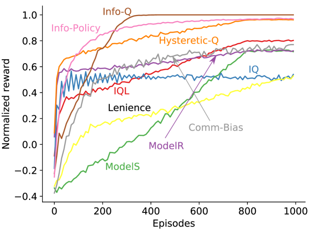
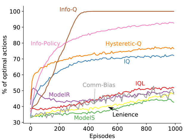
Figure 2: Normalized reward obtained during training, as a function of episodes in the climbing game. Info-Q converged to an optimal policy in around 300 episodes.

Figure 3: Percentage of optimal actions during training, as a function of episodes in the climbing game. The difference between the algorithms is magnified in this plot.

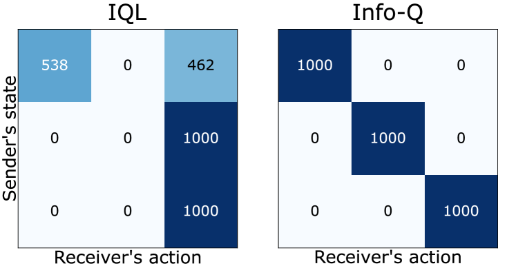
Figure 4: Counts of (state, action) pairs for IQL and Info-Q. With IQL, the receiver took $a_{3}$ in $s_{2}$, even though $a_{2}$ is the optimal action to take. With Info-Q, all runs converged to an optimal policy.

Figure 5: Venn diagram of messaging policy for IQL and Info-Q. Intersections in case of IQL imply that in some runs, multiple states were assigned the same message. In case of Info-Q, all states were assigned a distinct message.

Figure 3 shows the plot of the mean normalized reward, as a function of episodes. One standard error is shaded, but less than the line width in most cases. While some of the algorithms obtain rewards close to that obtained by Info-Q, the difference is magnified in Figure 3 which shows the percentage of runs that took the optimal actions, as a function of episodes.

For obtaining more insight into the potential issues of the baseline algorithms, we counted (state, action) pairs for each run. We iterated through the states, and for each state, we calculated the corresponding message sent by the sender and the action taken by the receiver. Figure 4 shows the matrix with the counts for each (state, action)-pair in case of Independent Q-Learning (IQL, on the left) and Info-Q (on the right). It can be observed that in state $s_{2}$ (middle row), the receiver takes inferior action $a_{3}$ (last column) with Q-Learning, whereas Info-Q takes optimal action $a_{2}$.

We also plotted Venn diagrams to visualize messaging policies. Figure 5 shows the Venn diagrams for independent Q-Learning and Info-Q. The region labeled $s_{i}$ outside of any intersection corresponds to runs in which $s_{i}$ was assigned a unique message. The intersection of regions $s_{i}$ and $s_{j}$ denote the runs in which $s_{i}$ and $s_{j}$ were assigned the same message. The intersection of all regions corresponds to runs in which all states were assigned the same message. Info-Q assigns a distinct message to each state, whereas some Q-Learning runs assign the same message to multiple states.

The combination of (state, action) pair counts and the Venn diagrams suggests that Q-Learning is converging to a sub-optimal policy of choosing $a_{3}$ in $s_{2}$. We hypothesize that this is due to the closeness of the two payoffs and the fact that $a_{3}$ is a “safer” action to take since the penalty is not high if the message was incorrect. The messages corresponding to $s_{2}$ and $s_{3}$ are the same in many runs. A possible reason for this is that, since the receiver is more likely to take $a_{3}$, there is insufficient incentive to send distinct messages for $s_{2}$ and $s_{3}$. We believe that this vicious cycle leads to the agents converging to a sub-optimal policy. Info-Q overcomes this cycle by forcing the sender to fully utilize the communication channel irrespective of the incentive it receives through the rewards. In Appendix C we present examples of hard 3x3 payoff matrices that support our intuition.

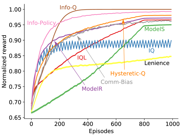
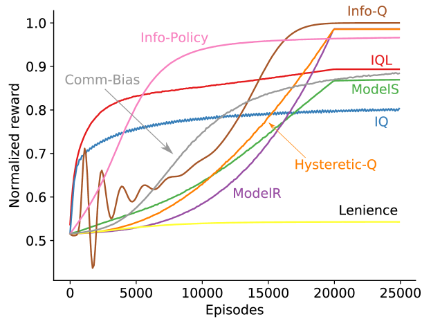
Figure 6: Mean normalized reward obtained during training, as a function of episodes, on random $3\!\times\!3$ payoff matrices.

Figure 7: Mean normalized reward obtained during training, as a function of episodes, on random $32\!\times\!32$ payoff matrices.

4.3 Results for Random Payoff Signaling Games

To ensure that the issues were not specific to a single game, we next conducted experiments on randomly generated payoff matrices of size $3\!\times\!3$ and $32\!\times\!32$. Figures 7 and 7 show the plots of the mean normalized reward, as a function of episodes, on $3\!\times\!3$ and $32\!\times\!32$ payoff matrices respectively. The mean, here, refers to all random payoff matrices and multiple runs for each matrix. One standard error of the mean is shaded, but less than the line width in most cases. Figures 9 and 9 show the boxplots of the percentage of runs that converge to an optimal policy for each payoff matrix of size $3\!\times\!3$ and $32\!\times\!32$ respectively. The boxplots clearly demonstrate the advantage of Info-Q compared to the other algorithms in terms of convergence to an optimal policy.

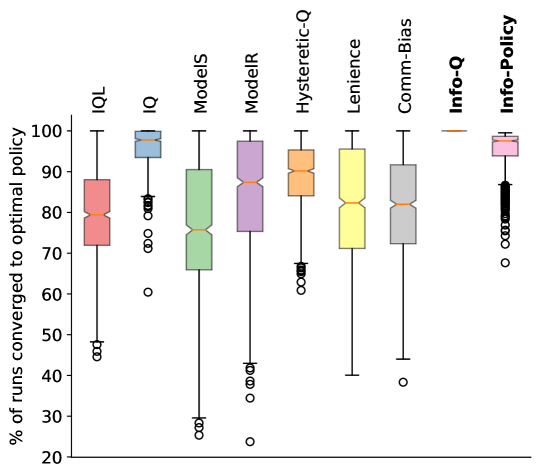
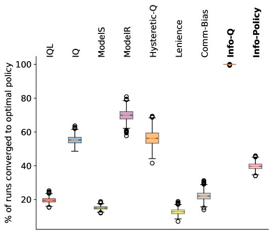
Figure 8: Boxplot of the percentage of runs that converged to an optimal policy for each $3\!\times\!3$ payoff matrix.

Figure 9: Boxplot of the percentage of runs that converged to an optimal policy for each $32\!\times\!32$ payoff matrix.

The version of our algorithm with the receiver being trained using policy gradient (Info-Policy) does not perform as well as Info-Q. This is due to the policy gradient method itself being slower to learn in this problem. Comm-Bias is also affected by it and performs worse than Info-Policy. IQ works fairly well in many problems since it is approximately equivalent to iterative best response. It fails in cases in which iterative best response converges to a sub-optimal policy. Since the agents explore more at the beginning of a period, the obtained reward is much lower. Hence, the reward curve for IQ does not truly reflect its test-time performance. Modeling the sender only works well if the receiver has access to the sender’s state during training (but still not as well as Info-Q). Otherwise, the performance is poor as shown in the plots. Modeling the receiver suffered from the issue of sub-optimal policy of the receiver. The best response by the sender to a sub-optimal receiver policy could be sub-optimal for the problem and vice versa, leading to the agents not improving. We postulate that the messages having no effect on the reward makes it harder for Hysteretic-Q and Lenience. The sender may receive the same reward for each of the messages it sends, leading to switching between messages for the same state and confusing the receiver.

5 Gridworld Experiments

We use the gridworld environment called “Treasure Hunt” introduced by Eccles et al. (2019) to test our algorithm in domains in which exact inference is infeasible (Figure 10). There are two agents in the environment with the goal of reaching the treasure at the bottom of one of the tunnels. Both agents have a limited field of view, and their positions make it so that one agent can easily see the goal location but cannot reach it, while the other agent can reach the goal, but potentially needs to explore all tunnels before reaching the goal. By allowing communication, one agent can easily locate the goal and signal the location to the other agent. Specifically, both the agents receive the message that the other agent sent at the previous time step. Hence, both agents take the role of a sender and a receiver, in contrast to the signaling game, in which there is only one sender and one receiver.

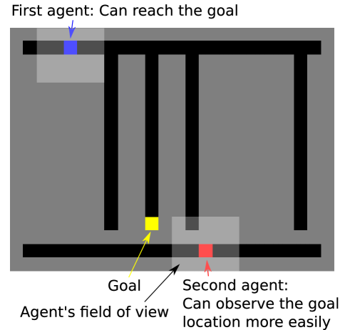
Figure 10: The Treasure Hunt environment.

Table 1: Comparison of our work with the biases given by Eccles et al. (2019)

Method	Final reward	Fraction of good runs
No-Bias (our implementation)	$11.55\pm 1.03$	$0.42$ $(5~{}/~{}12)$
No-Bias (Eccles et al. 2019)	$12.45\pm 0.48$	$0.28$ $(14~{}/~{}50)$
Positive signaling (our implementation)	$16.45\pm 0.20$	$1$ $(12~{}/~{}12)$
Positive signaling (Eccles et al. 2019)	$14.22\pm 0.36$	$0.84$ $(42~{}/~{}50)$
Positive signaling + listening (our implementation)	$16.25\pm 0.20$	$1$ $(12~{}/~{}12)$
Positive signaling + listening (Eccles et al. 2019)	$15.14\pm 0.33$	$0.94$ $(47~{}/~{}50)$
Inference-Based Messaging	$14.29\pm 1.26$	$0.92$ $(11~{}/~{}12)$
Inference-Based Messaging + positive listening	$15.48\pm 0.76$	$0.92$ $(11~{}/~{}12)$

We kept the core of the training algorithms including the neural network architecture used by Eccles et al. (2019) to make results comparable, and only modified the communication method. The agents choose messages to be sent by treating them as additional actions. We used a convolutional neural network followed by densely connected layers for feature extraction. An LSTM layer (Hochreiter and Schmidhuber 1997) over the features is used for dealing with partial observability, whose outputs are fed into linear layers for action and unscaled message logits and the value estimate. The action policy and the unscaled message policies of agents is updated using an off-policy policy gradient algorithm, IMPALA (Espeholt et al. 2018). Contrastive Predictive Coding (van den Oord, Li, and Vinyals 2018) is used to improve the LSTM performance. The experiments were run using the RLLib (Liang et al. 2018) library. In our method, the message selection uses inference simulation as shown in Algorithm 2 to compute $m^{(t)}=\operatorname*{\arg\!\max}_{m}p(s^{(t)}|m)$.

As a baseline, we used agents that picked messages based on the learned unscaled messaging policy and were trained independently using IMPALA (called No-Bias). We also compared our method with the biases given by Eccles et al. (2019). With positive signaling bias, the sender was incentivized into sending a message with higher information, using losses based on mutual information between private states and messages. With positive listening bias, the receiver was incentivized to use the received message for its action selection. It was achieved by maximizing the divergence between action probabilities resulting when messages are used and those when the messages are zeroed out. Each experiment was repeated 12 times and each run lasted for 300 million time steps. More details about the environment and the algorithms can be found in Appendix D.

5.1 Results

Table 1 shows the results we obtained for methods presented in Eccles et al. (2019) and our inference-based method. Similar to their paper, we divide the runs into two categories: good runs, in which the final reward is greater than 13, and all runs. Good runs require efficient communication since the max reward achieved without communication is 13 as shown by Eccles et al. (2019). Due to discrepancies in the results of our implementation of the communication biases and the values reported by Eccles et al. (2019), we provide both the values in the table. We believe that the difference in the number of repetitions for each experiment and the number of training steps to be the reason for these discrepancies. Due to computational constraints, we couldn’t perform longer runs or more repetitions.

Inference-based messaging performed significantly (more than one standard error of the mean difference) better than No-Bias. Adding positive listening bias further improved the performance of inference-based messaging. The performance of our method is similar to the reported value of positive signaling bias. Adding positive listening bias further improves our method, reaching a level similar to that of both signaling and listening biases. Agents receive more than 13 reward per episode after training in 11 of the 12 runs with inference-based messaging, which, as described earlier, shows that the agents are learning to communicate in most of the runs. Eccles et al. (2019) also show results of the social influence algorithm (Jaques et al. 2018) on this environment. The reported performance of social influence is nearly equal to that achieved by the no-bias baseline. Hence, our method significantly outperforms it too.

The results indicate that inference-based messaging can also improve communication in complex multi-agent environments, and be complementary to methods that improve the receiver.

6 Conclusions

The contributions of this paper are threefold. First, we demonstrated that state-of-the-art MARL algorithms often converge to sub-optimal policies in a signaling game. By analysing random payoff matrices we found that a sub-optimal payoff being close to the optimal payoff, in combination with the sub-optimal action having higher average payoffs in other states can lead to such behaviour.

We then proposed a method in which the sender simulates the receiver’s Bayesian inference of private state given a message to guide its message selection. Training agents with this new algorithm led to convergence to the optimal policy in nearly all runs, for a varied set of payoff matrices. The motivation to use the full communication channel irrespective of the reward appears to help learning agents to converge to the optimal policy.

Finally, we applied our method to a more complex gridworld problem which requires probability approximations for the inference simulation process. In this domain, too, we could show performance gains. However, we believe that with more sophisticated inference approximation techniques, the performance can be further improved.

Appendix: Supplementary Material

Appendix A Policy Updates in Algorithm 2

Algorithm 2 states that the policy parameters $\theta$ can be updated using any RL algorithm after off-policy correction. We use IMPALA (Espeholt et al. 2018) in our experiments. The policy gradient in the original IMPALA update is given by

$$\rho^{(t)}\nabla_{\theta}\log p(m^{(t)}|s^{(t)};\theta)(r^{(t)}+\gamma v^{(t+1)}-V_{\omega}(s^{(t)}))$$

$\rho^{(t)}$ in the above equations is the importance sampling weight to account for off-policy asynchronous actors. $v^{(t+1)}$ is the V-trace target computed similar to the original paper. $r^{(t)}$ is the current reward and $V_{\omega}(s^{(t)})$ is the value prediction given by the critic.

Since our agents use deterministic messaging policy while updating the unscaled messaging policy, the importance weight is given by $\rho^{(t)}=p(m^{(t)}|s^{(t)})~{}/~{}1$. Hence, the policy gradient becomes

$$\nabla_{\theta}p(m^{(t)}|s^{(t)};\theta)(r^{(t)}+\gamma v^{(t+1)}-V_{\omega}(s^{(t)}))$$

Appendix B Benchmark Algorithm Details

This section provides more detailed descriptions and parameter choices of the algorithms we compared our algorithm with in Section 4. Our selection includes traditional single-agent RL algorithms and algorithms from the literature that are shown to be effective in cooperative games with simultaneous actions. In particular, we consider:

$\bullet$ Info-Q – The information maximizing sender algorithm proposed in this paper. The sender uses Algorithm 1 and the receiver uses Q-Learning. All Q-values of the sender were initialized pessimistically (to -2) to prevent unwanted exploration by the sender. All Q-values of the receiver were initialized optimistically (to +2) to allow faster learning, but the same effect can be obtained by a higher step size. We used step size 0.1 and greedy action selection for the receiver. We found that $\epsilon$-greedy exploration by the receiver was not required for the signaling games we chose in this paper. The initial hyper-parameter guesses led to 100% convergence to optimal policy and hence, were not tuned further.

$\bullet$ Info-Policy – Similar to Info-Q, but the receiver uses a policy gradient method instead of Q-Learning. Updates to the receiver are performed using the REINFORCE update rule (Williams 1992) with the value of the state as baseline. Q-values of the sender were initialized pessimistically (to -2). The step size for both the policy update and the value baseline update was set to 0.5, while the step size for Q-value updates for the sender was set to 0.05. The receiver’s step size was tuned between $\{0.1,0.5\}$ and the sender’s step size was tuned between $\{0.5,0.05\}$.

$\bullet$ Fixed messages or fixed actions – For each algorithm, we ran a version in which the policy of either the sender or the receiver was fixed to an optimal one and only the other agent is trained. With this, the problem was reduced to a single-agent problem.

$\bullet$ Independent Q-Learning (IQL) – Both the sender and the receiver are trained independently using Q-Learning. The sender maintains a Q-table with entries for each state and each message, while the receiver maintains entries for each message and each action. For $3\!\times\!3$ payoffs, $\epsilon$-greedy, with initial $\epsilon$ of 0.3 and linear decay by $3.75\!\times\!10^{-4}$ per episode, was used for action selection, and step size ($\alpha$) 0.1 was used for the updates. For $32\!\times\!32$ payoffs, $\epsilon=0.1,\alpha=0.5$ were used, with $\epsilon$ decaying at a rate of $5\!\times\!10^{-6}$ per episode. $\alpha$ and initial $\epsilon$ were tuned among $\{0.01,0.05,0.1,0.5\}$ and $\{1,0.5,0.3,0.1\}$ respectively.

$\bullet$ Iterative Learning (IQ) – The learning is iterative, with the sender updating its policy for a certain number of episodes (denoted by ‘period’) while the receiver is fixed, followed by the receiver updating its policy while the sender is fixed, and so on. During each period, the updates for either the sender or the receiver are exactly the same as in independent Q-Learning. An agent doesn’t explore when its policy is fixed. When its policy is being trained, the action selection is $\epsilon$-greedy, with $\epsilon$ set to 1 at the beginning of the period and linearly decayed by 0.125 after every episode. Step size 0.5 was used for the updates and periods spanned 10 episodes. For $32\!\times\!32$ payoffs, periods spanned 100 episodes, and $\epsilon$ decay rate was 0.0125. Step size, initial $\epsilon$, and period were tuned among $\{0.01,0.05,0.1,0.5\}$, $\{1,0.5,0.3,0.1\}$, and $\{1,10,100\}$ respectively.

$\bullet$ Model the sender (ModelS) – The receiver maintains a Q-table for each state and each action. It also maintains a Q-table for each state and each message to model the sender. Based on the message sent by the sender and the model of the sender, the receiver calculates the posterior probabilities of each state ($p(s|m)$). The receiver assumes the true state to be the one with the highest probability, i.e., $\operatorname*{\arg\!\max}_{s}p(s|m)$, and the Q-table for states and actions is used to compute the best action as $\operatorname*{\arg\!\max}_{a}Q(s,a)$. $\epsilon$-greedy, with initial $\epsilon$ of 1 and linear decay by $1.25\!\times\!10^{-3}$ per episode was used for action selection, and step size 0.05 was used for all the updates. The $\epsilon$ decay rate was lowered to $5\!\times\!10^{-5}$, while the step size was increased to 0.1 in the case of $32\!\times\!32$ payoffs. Step size and initial $\epsilon$ were tuned among $\{0.01,0.05,0.1,0.5\}$ and $\{1,0.5,0.3,0.1\}$ respectively.

$\bullet$ Model the receiver (ModelR) – The sender maintains a Q-table for each state and each action. It also maintains a Q-table for each message and each action to model the receiver. The sender calculates the payoffs that would be obtained if the receiver follows the modeled policy and selects the message that maximizes this payoff (with $\epsilon$-greedy for exploration). This algorithm is similar to the one used by Sen, Airiau, and Mukherjee (2003), with the difference being that ModelR uses $\epsilon$-greedy w.r.t. max of Q-values instead of Boltzmann action selection w.r.t. expected Q-values since we empirically found that $\epsilon$-greedy performed better. An initial $\epsilon$ of 0.1 with linear decay of $1.25\!\times\!10^{-4}$ per episode was used for action selection, and step size 0.5 was used for all updates. For $32\!\times\!32$ payoffs, $\epsilon=1$, with a decay of $5\!\times\!10^{-5}$ per episode was used. Step size and initial $\epsilon$ were tuned among $\{0.01,0.05,0.1,0.5\}$ and $\{1,0.5,0.3,0.1\}$ respectively.

$\bullet$ Hysteretic-Q – An adaptation of the algorithm given by Matignon, Laurent, and Fort-Piat (2007) to our problems. The idea is to use higher step size for positive updates and lower step size for negative updates. $\epsilon$-greedy was used for exploration instead of Boltzmann exploration since we empirically found that $\epsilon$-greedy performed better for this problem. $\epsilon$ was initially set to 0.1 and linearly decayed by $1.25\!\times\!10^{-4}$ per episode. $\alpha=0.5$, $\beta=0.05$ were used as the step sizes for positive and negative updates respectively. Problems with $32\!\times\!32$ payoffs used $\epsilon=1$, which decayed by $5\!\times\!10^{-5}$ per episode. $\alpha$ and initial $\epsilon$ were tuned among $\{0.01,0.05,0.1,0.5\}$ and $\{1,0.5,0.3,0.1\}$ respectively, while $\beta$ was tuned among $\{0.1,1,10\}$ times $\alpha$.

$\bullet$ Lenience – An adaptation of the algorithm presented in Panait, Sullivan, and Luke (2006) (specifically the reinforcement learning version given by Wei and Luke (2016)). In the initial time steps, Q-values are updated only if the update is positive, ignoring low rewards. As the number of episodes increases, Q-values are always updated. Step size 0.1 was used for updates. Boltzmann action selection, with a maximum temperature of 5, a minimum temperature of $1.6\!\times\!10^{-3}$, and exponential temperature decay ($\delta$) by 0.99 per episode was used. The action selection moderation factor ($\omega$) and lenience moderation factor ($\theta$) were set to 0.1 and 1, respectively. The minimum temperature was lowered to 0 and $\theta$ was increased to 10 in case of $32\!\times\!32$ payoffs. Step size, $\delta$, maximum temperature, $\omega$ and $\theta$ were tuned among $\{0.01,0.05,0.1,0.5\}$, $\{0.999,0.995,0.99\}$, $\{5,50,500,5000\}$, $\{0.1,1,10\}$, $\{0.1,1,10\}$.

$\bullet$ Comm-Bias – Both the sender and the receiver are independently trained using REINFORCE. The sender additionally uses the positive signaling loss given by Eccles et al. (2019) during training. The auxiliary loss maximizes the mutual information between the sent message and the current state. We found that the receiver using the positive listening bias given by Eccles et al. (2019) didn’t improve the performance in these games. Since our experiments are in a tabular setting, we calculated the loss exactly at each timestep instead of averaging over a batch. A step size of 0.5 was used for policy updates. Positive signaling loss was given a weight of 0.01. The weight for average message entropy term ($\lambda$) was set to 0.1 in the $3\!\times\!3$ case and 0.3 in the $32\!\times\!32$ case, while the entropy target was set to 0.5 in the $3\!\times\!3$ case and 0 in the $32\!\times\!32$ case. Step size, positive signaling loss coefficient, $\lambda$, entropy target were tuned among $\{0.1,0.5\}$, $\{0.001,0.01,0.1\}$, $\{0.1,0.3,1.0\}$, $\{0.0,0.5,1.0,1.5\}$.

We selected hyper-parameters using a combination of grid search and manual tuning. We generated 100 random payoff matrices, and for each set of hyper-parameters and each payoff matrix, we repeated the experiment 1,000 times. The set of hyper-parameters with the highest percentage of runs that converged to the optimal policy was used in all other experiments. Hyper-parameter tuning was performed separately for 3x3 payoff matrices and 32x32 payoff matrices.

We generated 1,000 random payoff matrices to compare the algorithms. The best set of hyper-parameters was used for each algorithm, and the experiment was repeated 1,000 times. The mean of the normalized obtained rewards and percentage of the runs which converged to the optimal policy were recorded.

Appendix C Hard 3x3 Signaling Game Instances

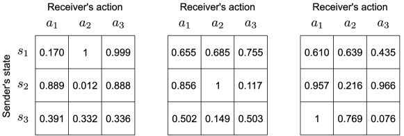
Figure 11: Three payoff matrices among the randomly generated ones that resulted in the lowest convergence-to-optimal percentage in terms of the mean over all algorithms.

Figure 12: Three payoff matrices among the randomly generated ones that resulted in the lowest final mean reward over all algorithms.

Figure 12 shows examples of some of the randomly generated $3\!\times\!3$ payoff matrices that were hard for the algorithms in terms of convergence to an optimal policy. The three matrices shown in the figure have the lowest mean percentage of convergence to an optimal policy across all the algorithms. Info-Q converges to an optimal policy in all the runs with these payoff matrices. Earlier, we hypothesized that the low percentage of convergence to optimal policy is due to the closeness in the payoffs of optimal and sub-optimal actions in a state, combined with a sub-optimal action having higher payoffs in other states. This hypothesis is strengthened by these payoff matrices since they too have the same issues. Multiple pairs of actions in the top game, $a_{1}$ and $a_{3}$ in $s_{3}$ in the middle game, and $a_{1}$ and $a_{3}$ in $s_{2}$ in the bottom game have close payoffs. In each case, the sub-optimal action has a higher expected payoff across all the states.

Since the sub-optimal payoffs are close to the optimal payoffs in these matrices, the algorithms still receive a high reward even when they are choosing a sub-optimal action. In contrast, the payoff matrices shown in Figure 12 lead to the algorithms receiving the lowest mean reward. While the percentage of runs that converge to the optimal policy is higher for these matrices, sub-optimal actions give much lower reward compared to the optimal ones. The mean final reward over all algorithms and all runs was around 0.9 for these matrices.

Appendix D Gridworld Experiment Details

D.1 Environment

The gridworld environment called “Treasure Hunt” is used in our experiments. The environment is kept exactly the same as that defined in the paper by Eccles et al. (2019) to keep the comparisons fair. For each training episode, an 18 high and 24 wide grid is created as below:

• Create two tunnels between the second column and the second to last column at the second and the second to last rows.

• Randomly choose four columns with a spacing of at least two columns between each of them. Create a tunnel of length 14 starting from the top tunnel in each of these columns.

• Place the first agent in a random cell in the top horizontal tunnel. Place the second agent in a random cell in the bottom horizontal tunnel.

• Place the goal at the bottommost cell of a random vertical tunnel.

The goal location is moved to the bottommost cell of a random vertical tunnel every time an agent reaches it. The episode terminates after 500 time steps and the grid is regenerated using the above rules.

At each time step, both agents observe a 5x5 area centered around their current location. The agents can move in any cardinal direction or take no action. The agents can also send a message that is shared with the other agent in the next time step. If an agent moves into a wall, it stays in its previous location. If it moves into the goal location, both agents get a reward of 1.

D.2 Training method

We trained agents using RLLib (Liang et al. 2018) library. The agents were trained in a decentralized manner using a modified version of RLLib’s implementation of the IMPALA algorithm. Both agents used their own neural network consisting of policy and value heads with the following architecture:

• Pass the $5\!\times\!5$ observations through a convolutional neural network (CNN) with 6 channels, kernel size of 1, and stride of 1.

• Flatten the CNN output and concatenate the received message. Pass it through two fully connected layers (MLP) with 64 units each.

• Concatenate the previous reward and action to the MLP output and pass it to an LSTM with 128 hidden units.

• Pass the LSTM outputs through a separate linear layer for action logits, message logits, and the value estimate.

Additionally, Contrastive Predictive Coding (CPC) (van den Oord, Li, and Vinyals 2018) objective was added to improve the LSTM performance. The CPC loss was calculated as follows:

• Transform the LSTM inputs by passing it through a linear layer with 64 outputs to get the input projection.

• Get the output projection corresponding to predictions of inputs at 20 future time steps by passing the LSTM outputs through 20 different linear layers with 64 outputs each.

• Compute the dot product of the output projection at time $t$ and input projection at time $t+k$ across all batches for $k=1,2,\ldots,20$.

• Calculate the CPC loss as the cross-entropy loss using the dot products as logits and the prediction being true when the input and output projections are from the same batch.

The hyper-parameters were selected using those used by Eccles et al. (2019) as the starting point and performing grid search over the hyper-parameters listed below. The other hyper-parameters were unchanged or manually chosen such that the mean episode reward after 100 million time steps was maximized. Each experiment was repeated 12 times and each run lasted for 300 million time steps. RMSProp optimizer (Hinton, Srivastava, and Swersky 2012) was used for updating the weights, with an initial learning rate of $10^{-3}$, exponentially decayed by 0.99 after every million steps. $\epsilon$ for the optimizer was set to $10^{-6}$. The optimizer was tuned between Adam (Kingma and Ba 2015) with a learning rate of $10^{-4}$ and no decay, Adam with a learning rate of $10^{-4}$ and exponential decay by 0.99 after every million steps, RMSProp with a learning rate of $10^{-4}$ and no decay, RMSProp with a learning rate of $10^{-3}$ and exponential decay by 0.99 after every million steps. RMSProp $\epsilon$ was further tuned between $\{10^{-6},10^{-3}\}$. All gradients were scaled such that the gradient norm was at most 10. The maximum gradient norm was tuned between $\{10,40\}$. Each rollout consisted of 100 time-steps and a batch size of 16 was used. 32 asynchronous parallel actors were used to collect data from the environment. The batch size was tuned between $\{16,32\}$, but rollout length was not tuned. Policy, value, and entropy losses were balanced by using a coefficient of 0.5 for the value loss and 0.006 for the entropy loss. The value loss coefficient was tuned between $\{0.5,1\}$, while the entropy loss coefficient was tuned among $\{0.01,0.006,0.001\}$. The discount factor was set to 0.99. The hyper-parameters for the positive signaling and positive listening biases were the same as those given by Eccles et al. (2019). For our method, the hyperparameter $\mu$ in Algorithm 2 was set to 0.5 after tuning among $\{0,0.25,0.5,0.9\}$.

The positive signaling and positive listening biases were implemented exactly as given by Eccles et al. (2019). The positive signaling loss is given by

$$\mathbb{E}(\lambda\mathcal{H}(p(m))-(\mathcal{H}(m|s)-\mathcal{H}_{target})^{2})$$

in which $\lambda$ and $\mathcal{H}_{target}$ are hyper-parameters, while $p(m)$ is calculated using the empirical average of the messaging policy probabilities over a rollout.

Positive listening loss is calculated in two steps. First, the policy of an agent without using messages from the other agent ($p(m|s^{\prime})$) is estimated by passing the observations, with the message from the other agent is set to zero (resulting in $s^{\prime}$), through the agent’s policy network to get the estimated policy $\hat{p}(m|s^{\prime})$. This estimate is trained by minimizing the loss

$$-\sum_{a}p(a|s)\log(\hat{p}(a|s^{\prime}))$$

by only backpropagating through the $\hat{p}(a|s^{\prime})$ term.

The distance between the policy which uses messages and the policy which doesn’t is maximized by minimizing the loss

$$-\sum_{a}|p(a|s)-\hat{p}(a|s^{\prime}))|$$

by only backpropagating through the $p(a|s)$ term.

The hyper-parameters used to balance these losses with the policy, value, and entropy losses, as well as those used in the calculation of the positive signaling loss are kept the same as those given by Eccles et al. (2019) for fair comparison.

References

- Balch and Arkin (1994) Balch, T. R.; and Arkin, R. C. 1994. Communication in Reactive Multiagent Robotic Systems. Autonomous Robots 1(1): 27–52.
- Bowling and Veloso (2000) Bowling, M.; and Veloso, M. 2000. An Analysis of Stochastic Game Theory for Multiagent Reinforcement Learning. Technical report, School of Computer Science, Carnegie-Mellon University.
- Bowling and Veloso (2002) Bowling, M.; and Veloso, M. 2002. Multiagent Learning Using a Variable Learning Rate. Artificial Intelligence 136(2): 215–250.
- Busoniu, Babuska, and Schutter (2008) Busoniu, L.; Babuska, R.; and Schutter, B. D. 2008. A Comprehensive Survey of Multiagent Reinforcement Learning. IEEE Trans. Syst. Man Cybern. Part C .
- Claus and Boutilier (1998) Claus, C.; and Boutilier, C. 1998. The Dynamics of Reinforcement Learning in Cooperative Multiagent Systems. In Proceedings of the Fifteenth National Conference on Artificial Intelligence and Tenth Innovative Applications of Artificial Intelligence Conference, 746–752.
- Crawford and Sobel (1982) Crawford, V. P.; and Sobel, J. 1982. Strategic information transmission. Econometrica: Journal of the Econometric Society 1431–1451.
- Eccles et al. (2019) Eccles, T.; Bachrach, Y.; Lever, G.; Lazaridou, A.; and Graepel, T. 2019. Biases for Emergent Communication in Multi-agent Reinforcement Learning. In Advances in Neural Information Processing Systems, 13111–13121.
- Espeholt et al. (2018) Espeholt, L.; Soyer, H.; Munos, R.; Simonyan, K.; Mnih, V.; Ward, T.; Doron, Y.; Firoiu, V.; Harley, T.; Dunning, I.; Legg, S.; and Kavukcuoglu, K. 2018. IMPALA: Scalable Distributed Deep-RL with Importance Weighted Actor-Learner Architectures. In Proceedings of the 35th International Conference on Machine Learning, 1406–1415.
- Evtimova et al. (2018) Evtimova, K.; Drozdov, A.; Kiela, D.; and Cho, K. 2018. Emergent Communication in a Multi-Modal, Multi-Step Referential Game. In Proceedings of the 6th International Conference on Learning Representations.
- Foerster et al. (2016) Foerster, J. N.; Assael, Y. M.; de Freitas, N.; and Whiteson, S. 2016. Learning to Communicate with Deep Multi-Agent Reinforcement Learning. In Advances in Neural Information Processing Systems, 2137–2145.
- Fulda and Ventura (2007) Fulda, N.; and Ventura, D. 2007. Predicting and Preventing Coordination Problems in Cooperative Q-learning Systems. In Proceedings of the 20th International Joint Conference on Artificial Intelligence, 780–785.
- Gibbons (1992) Gibbons, R. 1992. A Primer in Game Theory .
- He et al. (2015) He, K.; Zhang, X.; Ren, S.; and Sun, J. 2015. Delving Deep into Rectifiers: Surpassing Human-Level Performance on ImageNet Classification. In Proceedings of the IEEE International Conference on Computer Vision, 1026–1034.
- Hernandez-Leal, Kartal, and Taylor (2019) Hernandez-Leal, P.; Kartal, B.; and Taylor, M. E. 2019. A survey and critique of multiagent deep reinforcement learning. Autonomous Agents and Multi-Agent Systems 33(6): 750–797.
- Hinton, Srivastava, and Swersky (2012) Hinton, G.; Srivastava, N.; and Swersky, K. 2012. Neural Networks for Machine Learning Lecture 6a: Overview of Mini-Batch Gradient Descent. Coursera .
- Hochreiter and Schmidhuber (1997) Hochreiter, S.; and Schmidhuber, J. 1997. Long Short-Term Memory. Neural Computation 9(8): 1735–1780.
- Hoen et al. (2005) Hoen, P. J.; Tuyls, K.; Panait, L.; Luke, S.; and Poutré, J. A. L. 2005. An Overview of Cooperative and Competitive Multiagent Learning. In Learning and Adaption in Multi-Agent Systems, LAMAS.
- Jaques et al. (2018) Jaques, N.; Lazaridou, A.; Hughes, E.; Gülçehre, Ç.; Ortega, P. A.; Strouse, D.; Leibo, J. Z.; and de Freitas, N. 2018. Intrinsic Social Motivation via Causal Influence in Multi-Agent RL. CoRR abs/1810.08647.
- Kingma and Ba (2015) Kingma, D. P.; and Ba, J. 2015. Adam: A Method for Stochastic Optimization. In Proceedings of the 3rd International Conference on Learning Representations.
- Lazaridou, Peysakhovich, and Baroni (2017) Lazaridou, A.; Peysakhovich, A.; and Baroni, M. 2017. Multi-Agent Cooperation and the Emergence of (Natural) Language. In Proceedings of the 5th International Conference on Learning Representations.
- Liang et al. (2018) Liang, E.; Liaw, R.; Nishihara, R.; Moritz, P.; Fox, R.; Goldberg, K.; Gonzalez, J.; Jordan, M. I.; and Stoica, I. 2018. RLlib: Abstractions for Distributed Reinforcement Learning. In Proceedings of the 35th International Conference on Machine Learning, 3059–3068.
- Littman (1994) Littman, M. L. 1994. Markov Games as a Framework for Multi-Agent Reinforcement Learning. In Proceedings of the Eleventh International Conference on Machine Learning, 157–163.
- Lowe et al. (2019) Lowe, R.; Foerster, J. N.; Boureau, Y.; Pineau, J.; and Dauphin, Y. N. 2019. On the Pitfalls of Measuring Emergent Communication. In Proceedings of the 18th International Conference on Autonomous Agents and MultiAgent Systems, 693–701.
- Matignon, Laurent, and Fort-Piat (2007) Matignon, L.; Laurent, G. J.; and Fort-Piat, N. L. 2007. Hysteretic Q-Learning : An Algorithm for Decentralized Reinforcement Learning in Cooperative Multi-Agent Teams. In Proceedings of the International Conference on Intelligent Robots and Systems, 64–69.
- Matignon, Laurent, and Fort-Piat (2012) Matignon, L.; Laurent, G. J.; and Fort-Piat, N. L. 2012. Independent Reinforcement Learners in Cooperative Markov Games: A Survey Regarding Coordination Problems. The Knowledge Engineering Review 27(1): 1–31.
- Mnih et al. (2015) Mnih, V.; Kavukcuoglu, K.; Silver, D.; Rusu, A. A.; Veness, J.; Bellemare, M. G.; Graves, A.; Riedmiller, M. A.; Fidjeland, A.; Ostrovski, G.; Petersen, S.; Beattie, C.; Sadik, A.; Antonoglou, I.; King, H.; Kumaran, D.; Wierstra, D.; Legg, S.; and Hassabis, D. 2015. Human-Level Control Through Deep Reinforcement Learning. Nature 518(7540): 529–533.
- Omidshafiei et al. (2017) Omidshafiei, S.; Pazis, J.; Amato, C.; How, J. P.; and Vian, J. 2017. Deep Decentralized Multi-task Multi-Agent Reinforcement Learning under Partial Observability. In Proceedings of the 34th International Conference on Machine Learning.
- Palmer et al. (2018) Palmer, G.; Tuyls, K.; Bloembergen, D.; and Savani, R. 2018. Lenient Multi-Agent Deep Reinforcement Learning. In Proceedings of the 17th International Conference on Autonomous Agents and MultiAgent Systems.
- Panait and Luke (2005) Panait, L.; and Luke, S. 2005. Cooperative Multi-Agent Learning: The State of the Art. Auton. Agents Multi Agent Syst. .
- Panait, Sullivan, and Luke (2006) Panait, L.; Sullivan, K.; and Luke, S. 2006. Lenience Towards Teammates Helps in Cooperative Multiagent Learning. In Proceedings of the Fifth International Joint Conference on Autonomous Agents and Multi Agent Systems. Citeseer.
- Sen, Airiau, and Mukherjee (2003) Sen, S.; Airiau, S.; and Mukherjee, R. 2003. Towards a Pareto-Optimal Solution in General-Sum Games. In Proceedings of the Second International Joint Conference on Autonomous Agents and Multiagent Systems, 153–160.
- Shapley (1953) Shapley, L. S. 1953. Stochastic Games. Proceedings of the National Academy of Sciences 39(10): 1095–1100.
- Silver et al. (2018) Silver, D.; Hubert, T.; Schrittwieser, J.; Antonoglou, I.; Lai, M.; Guez, A.; Lanctot, M.; Sifre, L.; Kumaran, D.; Graepel, T.; Lillicrap, T.; Simonyan, K.; and Hassabis, D. 2018. A General Reinforcement Learning Algorithm that Masters Chess, Shogi, and Go Through Self-Play. Science 362(6419): 1140–1144. doi:10.1126/science.aar6404.
- Sukhbaatar, Szlam, and Fergus (2016) Sukhbaatar, S.; Szlam, A.; and Fergus, R. 2016. Learning Multiagent Communication with Backpropagation. In Advances in Neural Information Processing Systems 29.
- Sutton and Barto (2018) Sutton, R. S.; and Barto, A. G. 2018. Reinforcement Learning: An Introduction. MIT press.
- Tan (1993) Tan, M. 1993. Multi-Agent Reinforcement Learning: Independent vs. Cooperative Agents. In Proceedings of the Tenth International Conference on Machine Learning, 330–337.
- Tuyls and Weiss (2012) Tuyls, K.; and Weiss, G. 2012. Multiagent Learning: Basics, Challenges, and Prospects. AI Mag. .
- van den Oord, Li, and Vinyals (2018) van den Oord, A.; Li, Y.; and Vinyals, O. 2018. Representation Learning with Contrastive Predictive Coding. CoRR abs/1807.03748.
- Vinyals et al. (2019) Vinyals, O.; Babuschkin, I.; Czarnecki, W. M.; Mathieu, M.; Dudzik, A.; Chung, J.; Choi, D. H.; Powell, R.; Ewalds, T.; Georgiev, P.; et al. 2019. Grandmaster Level in StarCraft II Using Multi-Agent Reinforcement Learning. Nature 1–5.
- Wagner et al. (2003) Wagner, K.; Reggia, J. A.; Uriagereka, J.; and Wilkinson, G. 2003. Progress in the Simulation of Emergent Communication and Language. Adaptive Behaviour 11(1): 37–69.
- Watkins and Dayan (1992) Watkins, C. J.; and Dayan, P. 1992. Q-Learning. Machine Learning 8(3-4): 279–292.
- Wei and Luke (2016) Wei, E.; and Luke, S. 2016. Lenient Learning in Independent-Learner Stochastic Cooperative Games. Journal of Machine Learning Research 17: 84:1–84:42.
- Williams (1992) Williams, R. J. 1992. Simple Statistical Gradient-Following Algorithms for Connectionist Reinforcement Learning. Machine Learning 8: 229–256.
- Yang et al. (2004) Yang, X.; Liu, J.; Zhao, F.; and Vaidya, N. H. 2004. A Vehicle-to-Vehicle Communication Protocol for Cooperative Collision Warning. In Proceedings of the 1st Annual International Conference on Mobile and Ubiquitous Systems, 114–123.