Multi-institutional Collaborations for Improving Deep Learning-based Magnetic Resonance Image Reconstruction Using Federated Learning

Abstract

Fast and accurate reconstruction of magnetic resonance (MR) images from under-sampled data is important in many clinical applications. In recent years, deep learning-based methods have been shown to produce superior performance on MR image reconstruction. However, these methods require large amounts of data which is difficult to collect and share due to the high cost of acquisition and medical data privacy regulations. In order to overcome this challenge, we propose a federated learning (FL) based solution in which we take advantage of the MR data available at different institutions while preserving patients’ privacy. However, the generalizability of models trained with the FL setting can still be suboptimal due to domain shift, which results from the data collected at multiple institutions with different sensors, disease types, and acquisition protocols, etc. With the motivation of circumventing this challenge, we propose a cross-site modeling for MR image reconstruction in which the learned intermediate latent features among different source sites are aligned with the distribution of the latent features at the target site. Extensive experiments are conducted to provide various insights about FL for MR image reconstruction. Experimental results demonstrate that the proposed framework is a promising direction to utilize multi-institutional data without compromising patients’ privacy for achieving improved MR image reconstruction. Our code will be available at https://github.com/guopengf/FL-MRCM.

1 Introduction

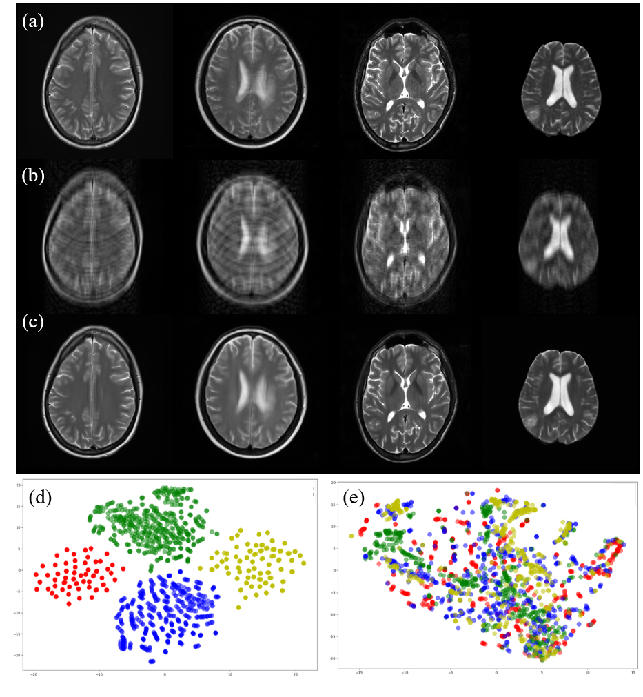
Figure 1: Top row: (a) ground truth, (b) zero-filled images, and (c) reconstructed images from the fastMRI [13], HPKS [10], IXI [3], and BraTS [26] datasets from left to right, respectively. Bottom row: t-SNE plots. The distribution of (d) latent features without cross-site modeling, and (e) latent features corresponding to the proposed cross-site modeling. In each plot, green, blue, yellow, and red dots represent data from fastMRI [13], HPKS [10], IXI [3], and BraTS [26] datasets, respectively.

Magnetic resonance imaging (MRI) is one of the most widely used imaging techniques in clinical applications. It is non-invasive and can be customized with different pulse sequences to capture different kinds of tissues. For instance, fat tissues are bright in $T_{1}$-weighted images, which can clearly show gray and white matter tissues in the brain. The radiofrequency pulse sequences used to make $T_{2}$-weighted images can delineate fluid from cortical tissue [11]. However, to increase the signal-to-noise ratio (SNR), clinical scanning usually involves the usage of multiple saturation frequencies and repeating acquisitions, which results in relatively long scan time. Various compressed sensing (CS) based methods have been proposed in the literature for accelerating the MRI sampling process by undersampling in the $k$-space during acquisition [4, 21, 22]. In recent years, data driven deep learning-based methods have been shown to produce superior performance on MR image reconstruction from partial $k$-space observations [20, 38, 39].

However, deep networks usually require large amounts of diversity-rich paired data which can be labor-intensive and prohibitively expensive to collect. In addition, one has to deal with patient privacy issues when storing them, making it difficult to share data with other institutions. Although deidentification [33] might provide a solution, building a large scale centralized dataset at a particular institution is still a challenging task.

The recently introduced federated learning (FL) framework [25, 36, 15] addresses this issue by allowing collaborative and decentralized training of deep learning-based methods. In particular, there is a server that periodically communicates with each institution to aggregate a global model and then shares it with all institutions. Each institution utilizes and stores its own private data. It is worth noting that instead of directly transferring data for training, the communication in FL algorithms only involves model parameters or update gradients, which resolves the privacy concerns. Hence, FL methods intrinsically facilitate multi-institutional collaborations between data centers (e.g., hospitals in the context of medical images).

However, the generalizability of models trained with the FL setting can still be suboptimal due to domain shift, which results from the data collected at multiple institutions with different sensors, disease types, and acquisition protocols, etc. This can be clearly seen from Fig. 1 where we show fully-sampled (Fig. 1(a)) and under-sampled (Fig. 1(b)) images from four different datasets. In Fig. 1(d), we visualize latent features corresponding to images from these datasets using t-Distributed Stochastic Neighbor Embedding (t-SNE) plot [23]. As can be seen from Fig. 1(d), features from a particular dataset are grouped together in a cluster indicating that each dataset has its own bias. As a result, we can see four different clusters of latent features. In order to make use of these datasets in the FL framework, one needs to align these features and remove the domain shift among the datasets. To circumvent this challenge, we propose a cross-site model for MR image reconstruction in which the learned intermediate latent features among different source sites are aligned with the distribution of the latent features at the target site. Specifically, the proposed method involves two optimization steps. In the first step, local reconstruction networks are trained on private data. In the second step, the intermediate latent features of the target domain data are transferred to other local source entities. An adversarial domain identifier is then trained to align the latent space distribution between the source domain and the target domain. Hence, minimizing the loss of adversarial domain identifier results in the reconstruction network weights being automatically adapted to the target domain. Fig. 1(e) and (c) show the distribution of aligned features and the corresponding reconstructed images in four datasets. The proposed cross-site modeling allows us to leverage datasets from various institutions for obtaining improved reconstructions.

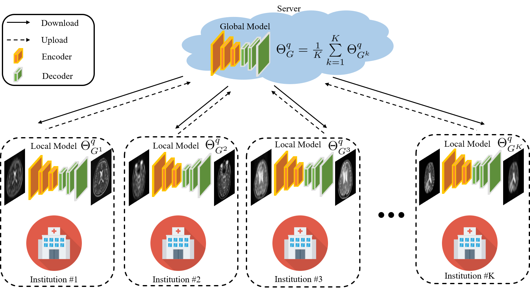
Figure 2: An overview of the proposed FL-MR framework. Through several rounds of communication between data centers and server, the collaboratively trained global model parameterized by $\Theta_{G}^{q}$ can be obtained in a data privacy-preserving manner.

To summarize, this paper makes the following contributions:

• A method called Federated Learning-based Magnetic Resonance Imaging Reconstruction (FL-MR) is proposed which enables multi-institutional collaborations for MRI reconstruction in a privacy-preserving manner.

• To address the domain shift issue among different sites, FL-MR with Cross-site Modeling (FL-MRCM) is proposed to align the latent space distribution between the source domain and the target domain.

• Extensive experiments are conducted to provide various insights about FL for MR image reconstruction.

2 Related Work

Reconstruction of MR images from under-sampled $k$-space data is an ill-posed inverse problem. In order to obtain a regularized solution, some priors are often used. CS-based methods make use of sparsity priors for recovering the image [21, 22] from partial $k$-space observations. In recent years, deep learning-based methods have been shown to produce superior performance on MR image reconstruction [12, 18, 31, 24, 40]. Some deep learning-based methods approach the problem by directly learning a mapping from the under-sampled data to the fully-sampled data in the image domain [38, 39, 14, 30]. Methods that learn a mapping in the $k$-space domain have also been proposed in the literature [1, 8].

Federated learning is a decentralized learning framework which allows multiple institutions to collaboratively learn a shared machine learning model without sharing their local training data  [2, 25, 27]. The FL training process consists of the following steps: (1) All institutions locally compute gradients and send locally trained network parameters to the server. (2) The server performs aggregation over the uploaded parameters from $K$ institutions. (3) The server broadcasts the aggregated parameters to $K$ institutions. (4) All institutions update their respective models with aggregated parameters and test the performance of the updated models. The institutions collaboratively learn a machine learning model with the help of a central cloud server  [42]. After a sufficient number of local training and update exchanges between the institutions and the server, a global optimal learned model can be obtained.

McMahan et al. [25] proposed FedAvg, which learns a global model by averaging model parameters from local entities. FedAvg [25] is one of the most commonly used frameworks for FL. FedProx [34] and Agnostic Federated Learning (AFL) [28] are extensions of FedAvg which attempt to address the learning bias issue of the global models for local entities. Recently, Sheller et al. [28] and Li et al. [16] proposed medical image segmentation models based on the FL framework. Peng et al. [29] proposed the federated adversarial alignment to mitigate the domain shift problem in image classification. In [17], Li et al. formulated a privacy-preserving pipeline for multi-institutional functional MRI classification and investigated different aspects of the communication frequency in federated models and privacy-preserving mechanisms. Although these methods [29, 17] achieved promising results to overcome domain shift in classification, due to the differences in network architectures, one cannot directly utilize them for MR image reconstruction. It is worth noting that the multi-institutional collaborative approach based on FL for MR image reconstruction has not been well studied in the literature.

3 Methodology

Similar to  [38, 39, 14, 30], the proposed method addresses the MR image reconstruction problem by directly learning a mapping from the under-sampled data to the fully-sampled data in the image domain. The MR image reconstruction process can be formulated as follows

$$x=F^{-1}(F_{d}y+\epsilon),$$ (1)

$$x,y\in\mathbb{C}^{N},$$

where $x$ denotes the observed under-sampled image, $y$ is the fully-sampled image, and $\epsilon$ denotes noise. Here, $F$ and $F^{-1}$ denote the Fourier transform matrix and its inverse, respectively. $F_{d}$ represents the undersampling Fourier encoding matrix that is defined as the multiplication of the Fourier transform matrix $F$ with a binary undersampling mask matrix. The acceleration factor (AF) controls the ratio of the amount of k-space data required for a fully-sampled image to the amount collected in an accelerated acquisition. The goal is to estimate $y$ from the observed under-sampled image $x$.

3.1 FL-based MRI Reconstruction

The proposed FL-MR framework is presented in Fig. 2 and Algorithm 1. Let $\mathcal{D}^{1},\mathcal{D}^{2},\dots,\mathcal{D}^{K}$ denote the MR image reconstruction datasets from $K$ different institutions. Each local dataset $\mathcal{D}^{k}$ contains pairs of under-sampled and fully-sampled images. At each institution, a local model is trained using its own data by iteratively minimizing the following loss

$$\mathcal{L}_{\text{recon}} =\sum\limits_{(x,y)\sim\mathcal{D}^{k}}\|G^{k}(x)-y\|_{1},$$ (2)

where $G^{k}$ corresponds to the local model at site $k$ and is parameterized by $\Theta_{G^{k}}$. $G^{k}(x)$ corresponds to the reconstructed image $\hat{y}$. After optimization with several local epochs (i.e. $P$ epochs) via

$$\Theta_{G^{k}}^{(p+1)}\leftarrow\Theta_{G^{k}}^{(p)}-\gamma\nabla\mathcal{L}_{\text{recon}},$$ (3)

each institution can obtain the trained FL-MR reconstruction model with the updated model parameters. Since each institution has its own data which may be collected by a particular sensor, disease type, and acquisition protocol, each $\mathcal{D}^{k}$ has a certain characteristic. Thus, when a local model is trained using its own data, it introduces a bias and does not generalize well to MR images from another institutions (see Fig. 1). One way to overcome this issue would be to train the network on a diverse multi-domain dataset by combining data from $K$ institutions as $\mathcal{D}=\{\mathcal{D}^{1}\cup\mathcal{D}^{2}\cup\dots\cup\mathcal{D}^{K}\}$ [7, 6, 5, 35, 41]. However, as discussed earlier, due to privacy concerns, this solution is not feasible and impedes multi-institutional collaborations in practice.

Input: $\mathcal{D}=\{\mathcal{D}^{1},\mathcal{D}^{2},\dots,\mathcal{D}^{K}\}$, datasets from K institution; P, the number of local epoches; Q, the number of global epoches; $\gamma$, learning rate; $G^{1},G^{2},\dots,G^{K}$, local models parameterized by $\Theta_{G^{1}},\Theta_{G^{2}},\dots,\Theta_{G^{K}}$; $G$, the global model parameterized by $\Theta_{G}$.

Output: well-trained global model $G$

$\triangleright$ parameters initialization;

for q = 1 to Q do

       for k = 1 to K in parallel do

             $\triangleright$ deploy weights to local model;

             for p = 1 to P do

                  

                  $\triangleright$ compute reconstruction loss $\mathcal{L}_{\text{recon}}$ with Eq. 2 and update parameters $\Theta_{G^{k}}$;

                  

             end for

            $\triangleright$ upload weights to server;

       end for

      $\triangleright$ update global model with Eq. 4;

end for

return $\Theta_{G}^{Q}$

Algorithm 1 FL-based MRI Reconstruction

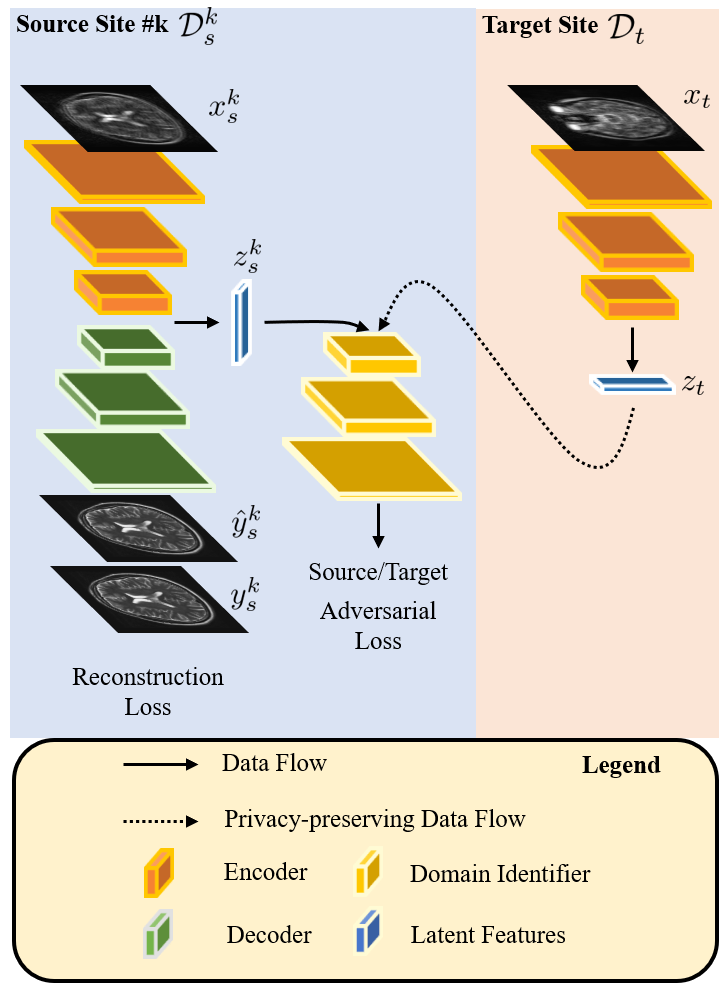
Figure 3: An overview of the proposed FL-MR framework with cross-site modeling in a source site.

To tackle this limitation and allow various sites to collaboratively train a MR image reconstruction model, we propose the FL-MR framework based on FedAVG [25]. Without accessing private data in each site, the proposed FL-MR method leverages a central server to utilize the information from other institutions by aggregating local model updates. The central server performs the aggregation of model updates by averaging the updated parameters from all local models as follows

$$\Theta_{G}^{q}=\frac{1}{K}\sum\limits_{k=1}^{K}\Theta_{G^{k}}^{q},$$ (4)

where $q$ represents the $q$-th global epoch. After $Q$ rounds of communication between local sites and central server, the trained global model parameterized by $\Theta_{G}^{Q}$, can leverage multi-domain information without directly accessing the private data in each institution.

3.2 FL-MR with Cross-site Modeling

Domain shift among datasets inevitably degrades the performance of machine learning models [19]. Existing works [9, 37] achieve superior performance by leveraging adversarial training. However, such methods require direct access to the source and target data, which is not allowed in FL-MR. Since we have multiple source domains and the data are stored in local institutions, training a single model that has access to source domains and target domain simultaneously is not feasible. Inspired by federated adversarial alignment [29] in classification tasks, we propose FL-MR with Cross-site Modeling (FL-MRCM) to address the domain shift problem in FL-based MRI reconstruction. As shown in Fig. 3, for a source site $\mathcal{D}_{s}^{k}$, we leverage the encoder part of the reconstruction networks ($E_{s}^{k}$) to project input onto the latent space $z^{k}_{s}$. Similarly, we can obtain $z_{t}$ for the target site $\mathcal{D}_{t}$. For each ($\mathcal{D}_{s}^{k}$, $\mathcal{D}_{t}$) source-target domain pair, we introduce an adversarial domain identifier $\mathcal{C}^{k}$ to align the latent space distribution between the source domain and the target domain. $\mathcal{C}^{k}$ is trained in an adversarial manner. Specifically, we first train $\mathcal{C}^{k}$ to identify which site the latent features come from. We then train the encoder part of the reconstruction networks to confuse $\mathcal{C}^{k}$. It should be noted that $\mathcal{C}^{k}$ only has access to the output latent features from $E_{s}^{k}$ and $E_{t}$, to maintain data sharing regulations. Given the k-th source site data $\mathcal{D}_{s}^{k}$ and the target site data $\mathcal{D}_{t}$, the loss function for $\mathcal{C}^{k}$ can be defined as follows

$$\mathcal{L}_{\text{adv}\mathcal{C}^{k}}= -\mathbb{E}_{x_{s}^{k}\sim\mathcal{D}_{s}^{k}}[\log\mathcal{C}^{k}(z^{k}_{s})]$$ (5)

$$-\mathbb{E}_{x_{t}\sim\mathcal{D}_{t}}[\log(1-\mathcal{C}^{k}(z_{t}))],$$

where $z^{k}_{s}=E_{s}^{k}(x_{s}^{k})$ and $z_{t}=E_{t}(x_{t})$. The loss function for encoders can be defined as follows

$$\mathcal{L}_{\text{adv}E^{k}}= -\mathbb{E}_{x_{s}^{k}\sim\mathcal{D}_{s}^{k}}[\log\mathcal{C}^{k}(z^{k}_{s})]-\mathbb{E}_{x_{t}\sim\mathcal{D}_{t}}[\log\mathcal{C}^{k}(z_{t})].$$ (6)

The overall loss function used for training the k-th source site with data $\mathcal{D}_{s}^{k}$ consists of the reconstruction and adversarial losses. It is defined as follows

$$\mathcal{L}_{\text{$\mathcal{D}_{s}^{k}$}}=\mathcal{L}_{\text{recon}}+\lambda_{\text{adv}}(\mathcal{L}_{\text{adv}\mathcal{C}^{k}}+\mathcal{L}_{\text{adv}E^{k}}),$$ (7)

where $\lambda_{\text{adv}}$ is a constant which controls the contribution of the adversarial loss. The detailed training procedure of FL-MRCM in a source site is presented in Algorithm 2. In supplementary material, we also provide the schematics of training FL-MRCM in a global view.

Input: $\mathcal{D}_{s}=\{\mathcal{D}^{1}_{s},\mathcal{D}^{2}_{s},\dots,\mathcal{D}^{K}_{s}\}$, data from the $K$ source institutions; $\mathcal{D}_{t}$, data from the target institution; $P$, the number of local epoches; $Q$, the number of global epoches; $\gamma$, learning rate; $\Theta_{G^{1}_{s}},...,\Theta_{G^{K}_{s}}$, parameters of the local models in the source sites; $\Theta_{\mathcal{C}^{1}},...,\Theta_{\mathcal{C}^{K}}$, domain identifiers; $\Theta_{G}$, the global model; $\Theta_{E_{t}}$, the encoder part of G in the target site.

$\triangleright$ parameters initialization

for q = 0 to Q do

       for k = 0 to K in parallel do

             $\triangleright$ deploy weights to local model

             for p = 0 to P do

                   Reconstruction:

                   $\triangleright$ compute reconstruction loss $\mathcal{L}_{\text{recon}}$ using Eq. 2

                   Cross-site Modeling:

                   $\triangleright$ compute adverisal loss $\mathcal{L}_{\text{adv}\mathcal{C}^{k}}$ and $\mathcal{L}_{\text{adv}E_{s}^{k}}$ using Eq. 5 and Eq. 6

                   $\triangleright$ compute the total loss using Eq. 7 and update $\Theta_{G_{s}^{k}}$, $\Theta_{\mathcal{C}^{k}}$, and $\Theta_{E_{t}}$

             end for

            $\triangleright$ upload weights to the central server

       end for

      $\triangleright$ update the global model using Eq. 4

      

end for

return $\Theta^{Q}_{G}$

Algorithm 2 FL-MR with Cross-site Modeling

3.3 Training and Implementation Details

We use U-Net [32] style encoder-decoder architecture for the reconstruction networks. Details of the network architecture are provided in supplementary material. $\lambda_{\text{adv}}$ is set equal to 1. Acceleration factor (AF) is set equal to 4. The network is trained using the Adam optimizer with the following hyperparameters: constant learning rate of $1\times 10^{-4}$ for the first 40 global epochs then $1\times 10^{-5}$ for the last global 10 epochs; 50 maximum global epochs; 2 maximum local epochs; batch size of 16. Hyperparameter selection is performed on the IXI validation dataset [3]. During training, the cross-sectional images are zero-padded or cropped to the size of 256 $\times$ 256.

4 Experiments and Results

In this section, we present the details of the datasets and various experiments conducted to demonstrate the effectiveness of the proposed framework. Specifically, we conduct experiments under two scenarios. Fig. 4 gives an overview of different training and evaluation strategies involved in the two scenarios. In Scenario 1, we analyze the effectiveness of improving the generalizability of the trained models using the proposed methods and other alternative strategies. Thus, the performance of a trained model is evaluated against a dataset that is not directly observed during training. In particular, we choose one dataset at a time to emulate the role of the user institution and consider data from other sites for training. This scenario is common in clinical practice. MRI scanners are usually equipped with accelerated acquisition techniques, so the user institution might not have access to fully-sampled data for training. In Scenario 2, we evaluate the proposed method by training it on the data from all available institutions to demonstrate the benefits of collaboration under the setting of federated learning. Rather than assuming that user institution does not have access to fully-sampled data, the training data split of user institution is also involved as a part of collaborations.

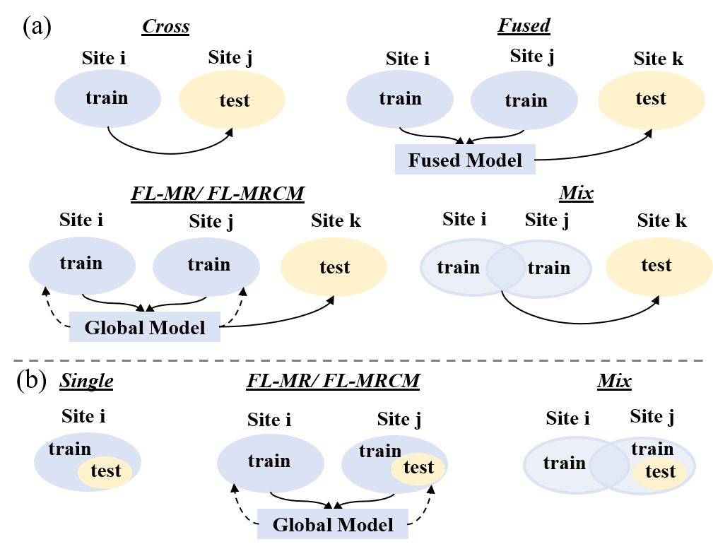
Figure 4: The schematic of different training strategies in (a) Scenario 1, and (b) Scenario 2. Note that for FL-MRCM, the source sites are the institutions that provide training data and the target site is the institution that provides testing data.

Table 1: Quantitative comparison with models trained by different strategies in Scenario 1.

Methods	Data Centers (Institutions)		$T_{1}$-weighted				$T_{2}$-weighted
	Train	Test	SSIM	PSNR	Average		SSIM	PSNR	Average
					SSIM	PSNR			SSIM	PSNR
Cross	F	B	0.9016	34.65	0.7907	30.02	0.9003	33.09	0.8296	29.51
	H	B	0.6670	29.12			0.8222	31.06
	I	B	0.8795	33.76			0.8610	31.36
	B	F	0.7694	28.61			0.7851	27.63
	H	F	0.8571	31.82			0.8682	29.04
	I	F	0.8417	31.18			0.8921	30.08
	B	H	0.5188	25.07			0.5898	26.28
	F	H	0.8402	28.52			0.8842	30.09
	I	H	0.6281	27.09			0.8583	29.45
	B	I	0.8785	30.10			0.7423	27.75
	F	I	0.9102	31.16			0.8917	29.57
	H	I	0.7968	29.16			0.8598	28.74
Fused	F, H, I	B	0.8672	33.98	0.8223	31.27	0.8696	32.73	0.8264	30.17
	B, H, I	F	0.8557	32.03			0.8524	29.19
	B, F, I	H	0.6615	27.87			0.7394	29.28
	B, F, H	I	0.9047	31.22			0.8441	29.47
FL-MR	F, H, I	B	0.9452	35.59	0.8976	32.09	0.916	33.76	0.8997	31.49
	B, H, I	F	0.9099	33.15			0.8991	30.86
	B, F, I	H	0.8249	28.49			0.8874	31.02
	B, F, H	I	0.9103	31.11			0.8962	30.32
FL-MRCM	F, H, I	B	0.9504	35.93	0.9108	32.51	0.9275	33.96	0.9113	31.77
	B, H, I	F	0.9149	33.31			0.9139	31.31
	B, F, I	H	0.8581	29.24			0.8978	31.35
	B, F, H	I	0.9197	31.54			0.9058	30.47
	F, H, I	B	0.9589	36.68	0.9182	32.96	0.9464	34.58	0.9260	32.44
Mix	B, H, I	F	0.9222	33.79			0.9239	31.89
(Upper Bound)	B, F, I	H	0.8630	29.19			0.9168	32.14
	B, F, H	I	0.9286	32.19			0.9169	31.14

4.1 Datasets

fastMRI [13] (F for short): $T_{1}$-weighted images corresponding to 3443 subjects are used for conducting experiments. In particular, data from 2583 subjects are used for training and remaining data from 860 subjects are used for testing. In addition, $T_{2}$-weighted images from 3832 subjects are also used, where data from 2874 subjects are used for training and data from 958 subjects are used for testing. For each subject, approximately 15 axial cross-sectional images that contain brain tissues are provided in this dataset.

HPKS [10] (H for short): This dataset is collected from post-treatment patients with malignant glioma. $T_{1}$ and $T_{2}$-weighted images from 144 subjects are analyzed, where 116 subjects’ data are used for training and 28 subjects’ data are used for testing. For each subject, 15 axial cross-sectional images that contain brain tissues are provided in this dataset.

IXI [3] (I for short): $T_{1}$-weighted images from 581 subjects are used, where 436 subjects’ data are used for training, 55 subjects’ data are used for validation, and 90 subjects’ data are used for testing. $T_{2}$-weighted images from 578 subjects are also analyzed, where 434 subjects’ data are used for training, 55 subjects’ data are used for validation and the remaining 89 subjects’ data are used for testing. For each subject, there are approximately 150 and 130 axial cross-sectional images that contain brain tissues for $T_{1}$ and $T_{2}$-weighted MR sequences, respectively.

BraTS [26] (B for short): $T_{1}$ and $T_{2}$-weighted images from 494 subjects are used, where 369 subjects’ data are used for training and 125 subjects’ data are used for testing. For each subject, approximately 120 axial cross-sectional images that contain brain tissues are provided for both MR sequences.

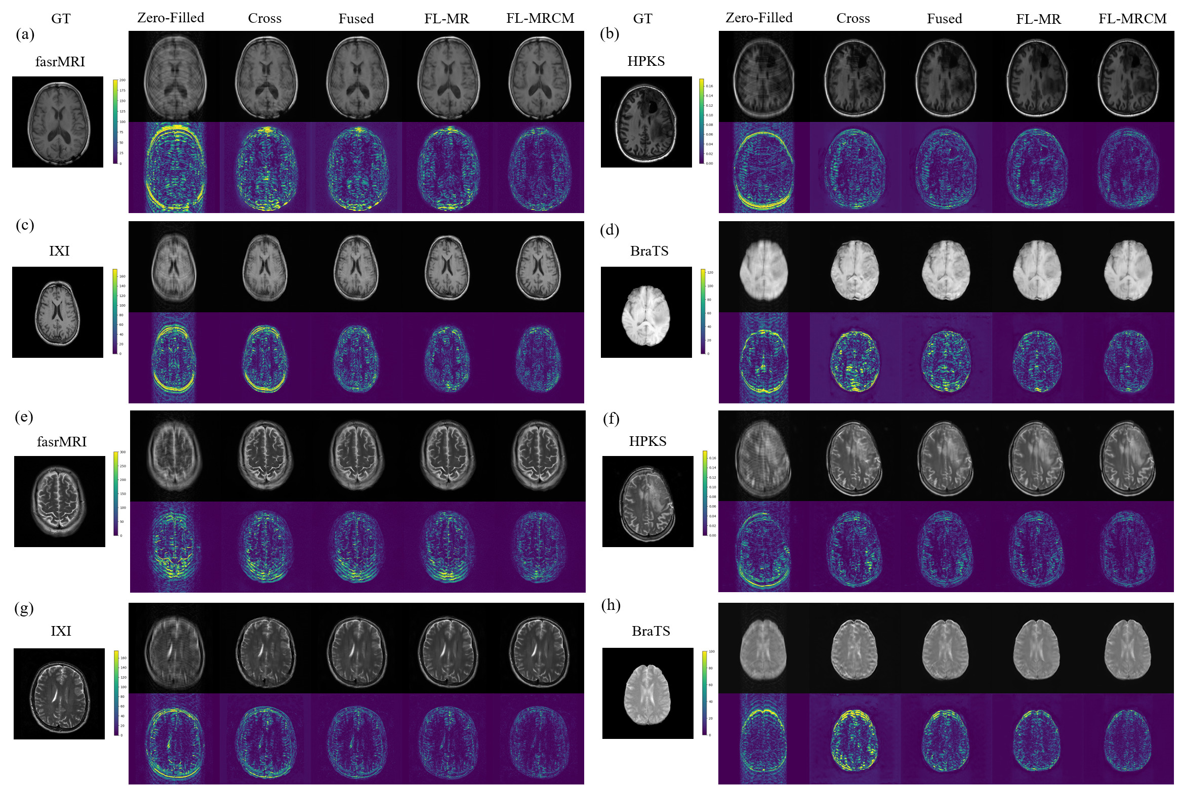
Figure 5: Qualitative results of different methods that correspond to Scenario 1. For results of $T_{1}$-weighted images on, (a) fastMRI [13], (b) HPKS [10], (c) IXI [3], (d) BraTS [26]. For results of $T_{2}$-weighted images on, (e) fastMRI [13], (f) HPKS [10], (g) IXI [3], (h) BraTS [26]. The second row of each sub-figure shows the absolute image difference between reconstructed images and the ground truth.

4.2 Evaluation of the Generalizability

In the first set of experiments (Scenario 1), we analyze the model’s generalizability to data from another site. In Table 1, we compare the quality of reconstructed images from different methods on four datasets using structural similarity index measure (SSIM) and peak-signal-to-noise ratio (PSNR). We first compare the performance of the proposed framework with models trained with data from a single data center. In this case, we obtain a trained model from one of the institutions and evaluate its performance on another data center in Table 1 under the label Cross. It is also possible to obtain multiple trained models from several institutions and fuse their outputs, which does not violate privacy regulations. In this case, we fuse the reconstructed images of the trained model from various institutions by calculating the average. The results corresponding to this strategy are shown in Table 1 under the label Fused. In addition, we can obtain a model that is trained with data from all available data centers, which is denoted by Mix in Table 1. However, this case compromises subjects’ privacy from other institutions, so we treat it as an upper bound.

As it can be seen from Table 1, our proposed FL-MR method exhibits better generalization and clearly outperforms other privacy-preserving alternative strategies. FL-MRCM further improves the reconstruction quality in each dataset by mitigating the domain shift. Fig. 5 shows the qualitative performance of different methods on $T_{1}$ and $T_{2}$-weighted images from four datasets. It can be observed that the proposed FL-MRCM method yields reconstructed images with remarkable visual similarity to the reference images compared to the other alternatives (see the last column of each sub-figure in Fig. 5) in four datasets with diverse characteristics.

Table 2: Quantitative comparison with models trained by different strategies in Scenario 2.

Methods	Data Centers		$T_{1}$-weighted				$T_{2}$-weighted
	(Institutions)
	Tain	Test	SSIM	PSRN	Average		SSIM	PSNR	Average
					SSIM	PSNR			SSIM	PSNR
Single	B	B	0.9660	37.30	0.9351	33.81	0.9558	34.90	0.9278	32.35
	F	F	0.9494	35.45			0.9404	32.43
	H	H	0.8855	29.67			0.9001	31.29
	I	I	0.9396	32.80			0.9151	30.79
FL-MR	B, F, H, I	B	0.9662	37.37	0.9294	33.92	0.9482	35.34	0.9238	32.64
		F	0.9404	35.25			0.9306	32.19
		H	0.8732	30.03			0.9021	31.74
		I	0.9379	33.03			0.9145	31.29
FL-MRCM	B, F, H, I	B	0.9676	37.57	0.9381	34.14	0.9630	35.85	0.9373	33.13
		F	0.9475	35.57			0.9385	32.69
		H	0.8940	30.27			0.9232	32.44
		I	0.9432	33.13			0.9244	31.54
	B, F, H, I	B	0.9698	37.62	0.9440	34.35	0.9655	35.83	0.9398	33.14
Mix		F	0.9558	36.15			0.9435	32.82
(Upper		H	0.9047	30.57			0.9236	32.47
Bound)		I	0.9454	33.08			0.9266	31.44

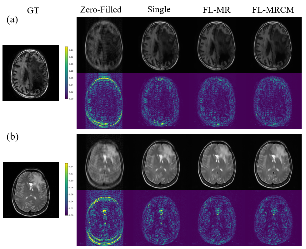
Figure 6: Qualitative results and error maps corresponding to different methods in Scenario 2 on HPKS [10]. (a) $T_{1}$- weighted, and (b) $T_{2}$-weighted images.

4.3 Evaluation of FL-based Collaborations

In the second set of experiments (Scenario 2), we analyze the effectiveness of our method to leverage data from all available institutions in a privacy-preserving manner. Since the goal is to evaluate the benefit of multi-institution collaborations, we compare the performance of the proposed framework with models trained with data from a single data center and evaluate on its own testing data, which is denoted by Single in Table 2. Similar to Scenario 1, we obtain a model that is directly trained with all available data, which is denoted by Mix in Table 2 and we treat it as an upper bound. It can be seen that the proposed FL-MRCM method outperforms the other methods and reaches the upper bound in term of SSIM and PSNR. It is worth noting that the multi-institution collaborations by the proposed FL-based method exhibits significant improvement on the smaller dataset. Specifically, on the HPKS [10], FL-MRCM improves SSIM from 0.9001 to 0.9232 and PSNR from 31.29 to 32.44 in $T_{2}$-weighted sequences. As shown in Fig. 6, the proposed methods have a better ability of suppressing errors around the skull and lesion regions, which is consistent with the quantitative results.

4.4 Ablation Study

The individual contribution of proposed cross-site modeling is demonstrated by a set of experiments (i.e. the comparison between FL-MR and FL-MRCM) in two scenarios under the setting of FL. Furthermore, we conduct a detailed ablation study to analyze the effectiveness of the proposed cross-site modeling without the FL framework. In this case, we obtain a trained model from one of the available sites and evaluate its performance on the data from another institution to observe the gain purely contributed by the cross-site modeling in Table 3. Sample reconstructed images are shown in Fig. 7. Experiments with cross-site modeling achieve smaller error. Due to space constraint, a similar ablation study on $T_{1}$-weighted images, more experimental results, and visualizations are provided in supplementary material.

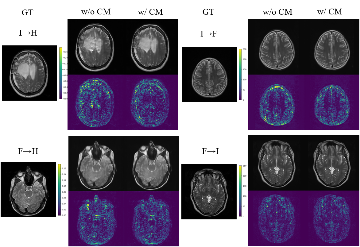
Figure 7: Qualitative comparisons and error maps on the $T_{2}$-weighted images using cross-site modeling (CM). I$\rightarrow$H represents the results from the model trained on I and tested on H, etc.

Table 3: Quantitative ablation study of the proposed cross-site modeling on the $T_{2}$-weighted images. For experiments with cross-site modeling, the target site is the institution that provides the test data.

Data Centers		w/o Cross-site Modeling				w/ Cross-site Modeling
(Institutions)		SSIM	PSNR	Average		SSIM	PSNR	Average
Train	Test			SSIM	PSNR			SSIM	PSNR
B	F	0.7851	27.63	0.7057	27.22	0.7914	27.85	0.7525	27.32
B	H	0.5898	26.28			0.6806	26.08
B	I	0.7423	27.75			0.7856	28.03
F	B	0.9003	33.09	0.8921	30.92	0.9139	33.84	0.9027	31.58
F	H	0.8842	30.09			0.8936	30.75
F	I	0.8917	29.57			0.9004	30.14
H	B	0.8222	31.06	0.8501	29.61	0.8391	31.54	0.8582	30.07
H	F	0.8682	29.04			0.8646	29.36
H	I	0.8598	28.74			0.8709	29.31
I	B	0.8610	31.36	0.8738	30.30	0.8946	32.11	0.8949	31.06
I	F	0.8921	30.08			0.9065	30.80
I	H	0.8583	29.45			0.8837	30.26

5 Conclusion

We present a FL-based framework to leverage multi-institutional data for the MR image reconstruction task in a privacy-preserving manner. To address the domain shift issue during collaborations, we introduce a cross-site modeling approach that provides the supervision to align the latent space distribution between the source domain and the target domain in each local entity without directly sharing the data. Through extensive experiments on four datasets with diverse characteristics, it is demonstrated that the proposed method is able to achieve better generalization. In addition, we show the benefits of multi-institutional collaborations under the FL-based framework in MR image reconstruction task.

References

- [1] Mehmet Akçakaya, Steen Moeller, Sebastian Weingärtner, and Kâmil Uğurbil. Scan-specific robust artificial-neural-networks for k-space interpolation (raki) reconstruction: Database-free deep learning for fast imaging. Magnetic resonance in medicine, 81(1):439–453, 2019.
- [2] Keith Bonawitz, Vladimir Ivanov, Ben Kreuter, Antonio Marcedone, H Brendan McMahan, Sarvar Patel, Daniel Ramage, Aaron Segal, and Karn Seth. Practical secure aggregation for privacy-preserving machine learning. In Proceedings of the 2017 ACM SIGSAC Conference on Computer and Communications Security, pages 1175–1191, 2017.
- [3] brain development.org.
- [4] Emmanuel J Candès, Justin Romberg, and Terence Tao. Robust uncertainty principles: Exact signal reconstruction from highly incomplete frequency information. IEEE Transactions on information theory, 52(2):489–509, 2006.
- [5] Pengfei Guo, Puyang Wang, Rajeev Yasarla, Jinyuan Zhou, Vishal M Patel, and Shanshan Jiang. Anatomic and molecular mr image synthesis using confidence guided cnns. IEEE Transactions on Medical Imaging, 2020.
- [6] Pengfei Guo, Puyang Wang, Rajeev Yasarla, Jinyuan Zhou, Vishal M Patel, and Shanshan Jiang. Confidence-guided lesion mask-based simultaneous synthesis of anatomic and molecular mr images in patients with post-treatment malignant gliomas. arXiv preprint arXiv:2008.02859, 2020.
- [7] Pengfei Guo, Puyang Wang, Jinyuan Zhou, Vishal M Patel, and Shanshan Jiang. Lesion mask-based simultaneous synthesis of anatomic and molecular mr images using a gan. In International Conference on Medical Image Computing and Computer-Assisted Intervention, pages 104–113. Springer, 2020.
- [8] Yoseo Han, Leonard Sunwoo, and Jong Chul Ye. k-space deep learning for accelerated mri. IEEE transactions on medical imaging, 39(2):377–386, 2019.
- [9] Judy Hoffman, Eric Tzeng, Taesung Park, Jun-Yan Zhu, Phillip Isola, Kate Saenko, Alexei Efros, and Trevor Darrell. Cycada: Cycle-consistent adversarial domain adaptation. In International conference on machine learning, pages 1989–1998. PMLR, 2018.
- [10] Shanshan Jiang, Charles G Eberhart, Michael Lim, Hye-Young Heo, Yi Zhang, Lindsay Blair, Zhibo Wen, Matthias Holdhoff, Doris Lin, Peng Huang, et al. Identifying recurrent malignant glioma after treatment using amide proton transfer-weighted mr imaging: a validation study with image-guided stereotactic biopsy. Clinical Cancer Research, 25(2):552–561, 2019.
- [11] Nikolaos L Kelekis et al. Hepatocellular carcinoma in north america: a multiinstitutional study of appearance on t1-weighted, t2-weighted, and serial gadolinium-enhanced gradient-echo images. AJR. American journal of roentgenology, 170(4):1005–1013, 1998.
- [12] Florian Knoll, Kerstin Hammernik, Chi Zhang, Steen Moeller, Thomas Pock, Daniel K Sodickson, and Mehmet Akcakaya. Deep-learning methods for parallel magnetic resonance imaging reconstruction: A survey of the current approaches, trends, and issues. IEEE Signal Processing Magazine, 37(1):128–140, 2020.
- [13] Florian Knoll, Jure Zbontar, Anuroop Sriram, Matthew J Muckley, Mary Bruno, Aaron Defazio, Marc Parente, Krzysztof J Geras, Joe Katsnelson, Hersh Chandarana, et al. fastmri: A publicly available raw k-space and dicom dataset of knee images for accelerated mr image reconstruction using machine learning. Radiology: Artificial Intelligence, 2(1):e190007, 2020.
- [14] Dongwook Lee, Jaejun Yoo, Sungho Tak, and Jong Chul Ye. Deep residual learning for accelerated mri using magnitude and phase networks. IEEE Transactions on Biomedical Engineering, 65(9):1985–1995, 2018.
- [15] Tian Li, Anit Kumar Sahu, Ameet Talwalkar, and Virginia Smith. Federated learning: Challenges, methods, and future directions. IEEE Signal Processing Magazine, 37(3):50–60, 2020.
- [16] Wenqi Li, Fausto Milletarì, Daguang Xu, Nicola Rieke, Jonny Hancox, Wentao Zhu, Maximilian Baust, Yan Cheng, Sébastien Ourselin, M Jorge Cardoso, et al. Privacy-preserving federated brain tumour segmentation. In International Workshop on Machine Learning in Medical Imaging, pages 133–141. Springer, 2019.
- [17] Xiaoxiao Li, Yufeng Gu, Nicha Dvornek, Lawrence Staib, Pamela Ventola, and James S Duncan. Multi-site fmri analysis using privacy-preserving federated learning and domain adaptation: Abide results. arXiv preprint arXiv:2001.05647, 2020.
- [18] Dong Liang, Jing Cheng, Ziwen Ke, and Leslie Ying. Deep mri reconstruction: Unrolled optimization algorithms meet neural networks. arXiv preprint arXiv:1907.11711, 2019.
- [19] Mingsheng Long, Yue Cao, Jianmin Wang, and Michael Jordan. Learning transferable features with deep adaptation networks. In International conference on machine learning, pages 97–105. PMLR, 2015.
- [20] Alexander Selvikvåg Lundervold and Arvid Lundervold. An overview of deep learning in medical imaging focusing on mri. Zeitschrift für Medizinische Physik, 29(2):102–127, 2019.
- [21] Michael Lustig, David Donoho, and John M Pauly. Sparse mri: The application of compressed sensing for rapid mr imaging. Magnetic Resonance in Medicine: An Official Journal of the International Society for Magnetic Resonance in Medicine, 58(6):1182–1195, 2007.
- [22] Shiqian Ma, Wotao Yin, Yin Zhang, and Amit Chakraborty. An efficient algorithm for compressed mr imaging using total variation and wavelets. In 2008 IEEE Conference on Computer Vision and Pattern Recognition, pages 1–8. IEEE, 2008.
- [23] Laurens van der Maaten and Geoffrey Hinton. Visualizing data using t-sne. Journal of machine learning research, 9(Nov):2579–2605, 2008.
- [24] Morteza Mardani, Enhao Gong, Joseph Y Cheng, Shreyas Vasanawala, Greg Zaharchuk, Marcus Alley, Neil Thakur, Song Han, William Dally, John M Pauly, et al. Deep generative adversarial networks for compressed sensing automates mri. arXiv preprint arXiv:1706.00051, 2017.
- [25] Brendan McMahan, Eider Moore, Daniel Ramage, Seth Hampson, and Blaise Aguera y Arcas. Communication-efficient learning of deep networks from decentralized data. In Artificial Intelligence and Statistics, pages 1273–1282. PMLR, 2017.
- [26] Bjoern H Menze et al. The multimodal brain tumor image segmentation benchmark (brats). IEEE transactions on medical imaging, 34(10):1993–2024, 2014.
- [27] Payman Mohassel and Peter Rindal. Aby3: A mixed protocol framework for machine learning. In Proceedings of the 2018 ACM SIGSAC Conference on Computer and Communications Security, pages 35–52, 2018.
- [28] Mehryar Mohri, Gary Sivek, and Ananda Theertha Suresh. Agnostic federated learning. arXiv preprint arXiv:1902.00146, 2019.
- [29] Xingchao Peng, Zijun Huang, Yizhe Zhu, and Kate Saenko. Federated adversarial domain adaptation. arXiv preprint arXiv:1911.02054, 2019.
- [30] Chen Qin, Jo Schlemper, Jose Caballero, Anthony N Price, Joseph V Hajnal, and Daniel Rueckert. Convolutional recurrent neural networks for dynamic mr image reconstruction. IEEE transactions on medical imaging, 38(1):280–290, 2018.
- [31] Saiprasad Ravishankar, Jong Chul Ye, and Jeffrey A Fessler. Image reconstruction: From sparsity to data-adaptive methods and machine learning. Proceedings of the IEEE, 108(1):86–109, 2019.
- [32] Olaf Ronneberger, Philipp Fischer, and Thomas Brox. U-net: Convolutional networks for biomedical image segmentation. In International Conference on Medical image computing and computer-assisted intervention, pages 234–241. Springer, 2015.
- [33] Joachim Roski, George W Bo-Linn, and Timothy A Andrews. Creating value in health care through big data: opportunities and policy implications. Health affairs, 33(7):1115–1122, 2014.
- [34] Anit Kumar Sahu, Tian Li, Maziar Sanjabi, Manzil Zaheer, Ameet Talwalkar, and Virginia Smith. On the convergence of federated optimization in heterogeneous networks. arXiv preprint arXiv:1812.06127, 3, 2018.
- [35] Veit Sandfort, Ke Yan, Perry J Pickhardt, and Ronald M Summers. Data augmentation using generative adversarial networks (cyclegan) to improve generalizability in ct segmentation tasks. Scientific reports, 9(1):1–9, 2019.
- [36] Micah J Sheller, G Anthony Reina, Brandon Edwards, Jason Martin, and Spyridon Bakas. Multi-institutional deep learning modeling without sharing patient data: A feasibility study on brain tumor segmentation. In International MICCAI Brainlesion Workshop, pages 92–104. Springer, 2018.
- [37] Eric Tzeng, Judy Hoffman, Trevor Darrell, and Kate Saenko. Simultaneous deep transfer across domains and tasks. In Proceedings of the IEEE International Conference on Computer Vision, pages 4068–4076, 2015.
- [38] Puyang Wang, Eric Z Chen, Terrence Chen, Vishal M Patel, and Shanhui Sun. Pyramid convolutional rnn for mri reconstruction. arXiv preprint arXiv:1912.00543, 2019.
- [39] Puyang Wang, Pengfei Guo, Jianhua Lu, Jinyuan Zhou, Shanshan Jiang, and Vishal M Patel. Improving amide proton transfer-weighted mri reconstruction using t2-weighted images. In International Conference on Medical Image Computing and Computer-Assisted Intervention, pages 3–12. Springer, 2020.
- [40] Shanshan Wang, Ziwen Ke, Huitao Cheng, Sen Jia, Leslie Ying, Hairong Zheng, and Dong Liang. Dimension: Dynamic mr imaging with both k-space and spatial prior knowledge obtained via multi-supervised network training. NMR in Biomedicine, page e4131, 2019.
- [41] Wenjun Yan, Lu Huang, Liming Xia, Shengjia Gu, Fuhua Yan, Yuanyuan Wang, and Qian Tao. Mri manufacturer shift and adaptation: Increasing the generalizability of deep learning segmentation for mr images acquired with different scanners. Radiology: Artificial Intelligence, 2(4):e190195, 2020.
- [42] Qiang Yang, Yang Liu, Tianjian Chen, and Yongxin Tong. Federated machine learning: Concept and applications. ACM Transactions on Intelligent Systems and Technology (TIST), 10(2):1–19, 2019.