Abstract

The primary objective of this scholarly work is to develop two estimation procedures – maximum likelihood estimator (MLE) and method of trimmed moments (MTM) – for the mean and variance of lognormal insurance payment severity data sets affected by different loss control mechanism, for example, truncation (due to deductibles), censoring (due to policy limits), and scaling (due to coinsurance proportions), in insurance and financial industries. Maximum likelihood estimating equations for both payment-per-payment and payment-per-loss data sets are derived which can be solved readily by any existing iterative numerical methods. The asymptotic distributions of those estimators are established via Fisher information matrices. Further, with a goal of balancing efficiency and robustness and to remove point masses at certain data points, we develop a dynamic MTM estimation procedures for lognormal claim severity models for the above-mentioned transformed data scenarios. The asymptotic distributional properties and the comparison with the corresponding MLEs of those MTM estimators are established along with extensive simulation studies. Purely for illustrative purpose, numerical examples for 1500 US indemnity losses are provided which illustrate the practical performance of the established results in this paper.

Keywords & Phrases. Dynamic Estimation; Lognormal Insurance Severity; Maximum Likelihood Estimators; Trimmed Moments; Insurance Payments; Loss Models; Robust Estimation; Truncated and Censored Data.

1 Introduction

The research leading to the results of this work is basically motivated to find and compare two estimation approaches for two types of insurance benefit payment severity data with the assumption of stand-alone continuous underlying loss distributions. In practice, due to commonly used loss control mechanism in the financial and insurance industries (Ergashev et al., 2016, Klugman et al., 2019), the random variables we observe and wish to model are affected by data truncation (due to deductibles), censoring (due to policy limits), and scaling (due to coinsurance factor). Therefore, the main focus of this paper is to develop maximum likelihood and a dynamic method of trimmed moments estimators, respectively, called MLE and MTM for short, of location and scale parameters of lognormal insurance benefit payment claims severity.

In the current practice, statistical inference for loss models is almost exclusively likelihood based (see, e.g., Klugman et al., 2019), which typically result in sensitive loss severity models if there is a small perturbation in the underlying assumed model or if the observed sample is coming from a contaminated distribution, Tukey (1960). Further, following the work by Cooray and Ananda (2005), the contemporary actuarial loss modeling literature has been directed toward composite loss modeling (see, e.g., Abu Bakar et al., 2015, Chan et al., 2018, Scollnik, 2007, Scollnik and Sun, 2012) which is also referred to as splicing (see, e.g., Klugman et al., 2019) including mixtures of Erlangs (see, e.g., Gui et al., 2021, Reynkens et al., 2017, Verbelen et al., 2015). The composite models appear to capture the tail behavior of the underlying distribution more accurately (see, e.g., Grün and Miljkovic, 2019, and the references therein). But as mentioned by Punzo et al. (2018), often the simple closed-form expressions for the pdf of composite models are not available which could lead to more complexity of deriving analytic sampling distributional results. Therefore, beside many ideas from the mainstream robust statistics literature (see, e.g., Hampel, 1974, Huber, 1964, Huber and Ronchetti, 2009), actuaries have to deal with heavy-tailed and skewed distributions, data truncation and censoring, identification and recycling of outliers, and aggregate loss, etc. Thus, it is appealing to search some estimation procedures which directly work with those mentioned loss control mechanism, are insensitive against small perturbations from the assumed models, computationally efficient, and still reasonably balance the asymptotic efficiency-robustness trade-offs with respect to the corresponding MLE.

As a member of log-location-scale family, the lognormal distribution has diverse applications in actuarial science, business, and economics (see, e.g., Serfling, 2002, and the references therein) which closely approximates certain types of homogeneous actuarial loss data (Hewitt et al., 1979, Punzo et al., 2018). Further, it has been established that, even for the heterogeneous actuarial losses, lognormal distribution is able to capture the nature of the data set either on the head or on the tail or on both head and tail parts of different composite models, see, for example, Cooray and Ananda (2005), Brazauskas and Kleefeld (2016), Miljkovic and Grün (2016), Punzo et al. (2018), Blostein and Miljkovic (2019), and Michael et al. (2020). More comprehensive investigation of 256 different composite models have been analyzed by Grün and Miljkovic (2019).

On the other hand, MTM approach can be viewed as a special case of $L$-statistics (Chernoff et al., 1967) and has established itself as sufficiently general and flexible in order to balance between estimator’s efficiency and robustness for fitting of continuous parametric models based on complete ground-up loss severity data (see, e.g., Brazauskas et al., 2009, Zhao et al., 2018). But it is yet open to investigate the MTM performance beyond the complete data scenario and this paper will address this issue for lognormal payment-per-payment and payment-per-loss data scenarios. If a truncated (both singly and doubly) normal sample data set is available then the MLE procedures for such data have been developed by Cohen (1950) and the method of moments estimators can be found in Cohen (1951) and Shah and Jaiswal (1966). A novel robust estimation procedure called method of truncated moments (MTuM) for modeling different actuarial loss data scenarios is initially purposed by Poudyal (2018) and further developed by Poudyal (2021). But the goal and motivation of this research work is different. That is, instead of fitting composite models or designing MTuM, both MLE and MTM estimation procedures will be derived for stand-alone lognormal insurance benefit payment data scenarios with an assumption that a close fit in one tail or both tails of the distribution is not desired but at the same time we want to remove partial point masses accumulated at the truncated and/or censored data points. As the main contribution of this parer, asymptotic distributions, such as normality and consistency, along with asymptotic relative efficiency (ARE) of those estimators (under transformed data) with respect to the corresponding MLEs are established including extensive validating simulation studies. The developed methodologies in this paper are implemented with real 1500 US indemnity loss data set. It will be shown that, when properly redesigned, a dynamic MTM can be a robust and computationally efficient alternative to the MLE-based inference for claim severity models that are affected by deductibles, policy limits, and coinsurance. Some of the technical challenges in implementing the developed estimation procedures in practical data analysis are discussed along with the corresponding simplifying assumptions.

The remainder of the paper is organized as follows. In Section 2, we describe the two types of insurance benefit payment lognormal random variables. In Section 3, the MLE procedures is developed for those two payment type of data sets with their corresponding asymptotic distributional properties. Section 4 is the corresponding section to develop dynamic MTM procedures for the location and scale parameters for those two payment models. Comparison of ARE of those MTM estimators with respect to MLE are also presented. Section 5 is for some special cases which are more common in operational risk modeling with some theoretical results. Section 6 summarizes a detail simulation study. Numerical examples to observe the performance of the developed estimation procedures can be found in Section 7. Finally, summary and concluding remarks are offered in Section 8.

2 Insurance Payments

Consider a ground-up lognormal loss random variable $W\sim LN(w_{0},\theta,\sigma)$ with cdf

$$F_{W}(w) =\Phi\left(\dfrac{\log{(w-w_{0}})-\theta}{\sigma}\right),\quad w>w_{0},\ -\infty<\theta<\infty,\ \sigma>0,$$ (2.1)

where $\theta$ and $\sigma$ are unknown parameters to be estimated, $w_{0}>0$ is assumed to be known, and $\Phi$ is the cdf of the standard normal distribution. Clearly $X:=\log{(W-w_{0})}\sim N(\theta,\sigma^{2})$ with cdf and pdf, respectively, given by:

$$F_{X}(x)=\Phi\left(\frac{x-\theta}{\sigma}\right)\quad\mbox{and}\quad f_{X}(x)=\frac{1}{\sigma}\phi\left(\frac{x-\theta}{\sigma}\right),\qquad-\infty<x<\infty,$$ (2.2)

where $\phi(x)=\left(1/\sqrt{2\pi}\,\right)e^{-x^{2}/2},\ x\in\mathbb{R}$ is the pdf of the standard normal distribution. The corresponding quantile function $F_{X}^{-1}:(0,1)\to\mathbb{R}$ is given by $F_{X}^{-1}(v)=\theta+\sigma\Phi^{-1}(v).$

Insurance contracts have coverage modifications that need to be taken into account when modeling the underlying loss variable. Usually the coverage modifications such as deductibles, policy limits, and coinsurance are introduced as loss control strategies so that unfavorable policyholder behavioral effects (e.g., adverse selection) can be minimized. There are also situations when certain features of the contract emerge naturally (e.g., the value of insured property in general insurance is a natural upper policy limit). Here we describe two common transformations of the loss variable along with the corresponding cdfs, pdfs, and qfs.

Suppose the lognormal severity random variable $W$ has ordinary deductible $d$, upper policy limit $u$, and coinsurance factor $c$ ($0<c\leq 1$). These coverage specifications imply that when a loss $W$ is reported, the insurance company is responsible for a proportion $c$ of $W$ exceeding $d$, but no more than $c(u-d)$. Define

$$t:=\log{(d-w_{0})},\ T:=\log{(u-w_{0})},\ R:=T-t,\ \gamma:=\frac{t-\theta}{\sigma},\ \mbox{and}\ \xi:=\frac{T-\theta}{\sigma}.$$ (2.3)

and note that it is possible to have $t<0$ but $d>0$. Here, it is important to note that $d$ and $u$ refer for the lognormal left-truncation threshold and right-censored point, respectively. On the other hand, $t$ and $T$ are, respectively, the corresponding normal form of left-truncation threshold and right censored point as defined in (2.3). Then, obviously

$$\theta =t-\sigma\gamma\quad\mbox{and}\quad\xi=\gamma+\frac{R}{\sigma}.$$ (2.4)

Also, let $\bar{\Phi}(z)=1-\Phi(z)$ be the standard normal survival function at $z\in\mathbb{R}$. Finally, define

$$\Omega_{1} :=\frac{\phi(\gamma)}{\bar{\Phi}(\gamma)-\bar{\Phi}(\xi)}\quad\mbox{and}\quad\Omega_{2}:=\frac{\phi(\xi)}{\bar{\Phi}(\gamma)-\bar{\Phi}(\xi)}.$$ (2.5)

Now, if the loss severity $W$ below the deductible $d$ is completely unobservable (even its frequency is unknown), then the left-truncated, right-censored, and linearly transformed (also known as payment-per-payment variable) form of $W$ is defined as:

$$Y_{w}:=c\left(\min\big{\{}W,u\big{\}}-d\right)\,|\,W>d=\left\{\begin{array}[]{ll}\mbox{undefined},&W\leq d;\\ c\left(W-d\right),&d<W<u;\\ c\left(u-d\right),&u\leq W.\\ \end{array}\right.$$ (2.6)

The corresponding normal form of $Y_{w}$ is given by

$$Y:=c\log{\left(\dfrac{Y_{w}}{c(d-w_{0})}+1\right)}=c\left(\min\big{\{}X,T\big{\}}-t\right)\,|\,X>t=\left\{\begin{array}[]{ll}\mbox{undefined},&X\leq t;\\ c\left(X-t\right),&t<X<T;\\ c\left(T-t\right),&T\leq X.\\ \end{array}\right.$$ (2.7)

The cdf $F_{Y}$, pdf $f_{Y}$, and qf $F_{Y}^{-1}$ of the payment-per-payment random variable $Y$ are given by:

$$F_{Y}(y;\,c,t,T)=\mbox{\bf P}\left[c\left(\min\big{\{}X,\,T\big{\}}-t\right)\leq y\,\big{|}\,X>t\right]=\left\{\begin{array}[]{ll}0,&y\leq 0;\\[2.15277pt] \frac{F_{X}(y/c+t)-F_{X}(t)}{1-F_{X}(t)},&0<y<c(T-t);\\[2.15277pt] 1,&y\geq c(T-t),\\ \end{array}\right.$$ (2.8)

$$f_{Y}(y;\,c,t,T)=\left\{\begin{array}[]{ll}\frac{f_{X}(y/c+t)}{c[1-F_{X}(t)]},&0<y<c(T-t);\\[4.30554pt] \frac{1-F_{X}(T^{-})}{1-F_{X}(t)},&y=c(T-t);\\[3.22916pt] 0,&\mbox{elsewhere},\\ \end{array}\right.$$ (2.9)

and

$$F_{Y}^{-1}(v;\,c,t,T)=\left\{\begin{array}[]{ll}c\left[F_{X}^{-1}\big{(}v+(1-v)F_{X}(t)\big{)}-t\right],&0\leq v<\frac{F_{X}(T)-F_{X}(t)}{1-F_{X}(t)};\\[3.22916pt] c(T-t),&\frac{F_{X}(T)-F_{X}(t)}{1-F_{X}(t)}\leq v\leq 1.\\ \end{array}\right.$$ (2.10)

The scenario that no information is available about $W$ below $d$ is likely to occur when modeling is done based on the data acquired from a third party (e.g., data vendor). For payment data collected in house, the information about the number of policies that did not report claims (equivalently, resulted in a payment of 0) would be available. This minor modification yields different payment variable, say $Z_{w}$, which can be treated as interval-censored and linearly transformed $W$ (also called payment-per-loss random variable):

$$Z_{w}:=c\left(\min\big{\{}W,u\big{\}}-\min\big{\{}W,d\big{\}}\right)=\left\{\begin{array}[]{ll}0,&W\leq d;\\ c\left(W-d\right),&d<W<u;\\ c\left(u-d\right),&u\leq W.\\ \end{array}\right.$$ (2.11)

The corresponding normal form of $Z_{w}$ is given by:

$$Z:=c\log{\left(\dfrac{Z_{w}}{c(d-w_{0})}+1\right)}=c\left(\min\big{\{}X,T\big{\}}-\min\big{\{}X,t\big{\}}\right)=\left\{\begin{array}[]{ll}0,&X\leq t;\\ c\left(X-t\right),&t<X<T;\\ c\left(T-t\right),&T\leq X.\\ \end{array}\right.$$ (2.12)

The cdf $F_{Z}$, pdf $f_{Z}$, and qf $F_{Z}^{-1}$ are related to $F_{X}$, $f_{X}$, and $F_{X}^{-1}$ and given by:

$$F_{Z}(z;\,c,t,T)=\mbox{\bf P}\left[c{\small\left(\min\big{\{}X,T\big{\}}-\min\big{\{}X,t\big{\}}\right)}\leq z\right]=\left\{\begin{array}[]{ll}0,&z<0;\\[1.07639pt] F_{X}(z/c+t),&0\leq z<c(T-t);\\[1.07639pt] 1,&z\geq c(T-t),\\ \end{array}\right.$$ (2.13)

$$f_{Z}(z;\,c,t,T)=\left\{\begin{array}[]{ll}F_{X}(t),&z=0;\\[1.07639pt] f_{X}(z/c+t)/c,&0<z<c(T-t);\\[1.07639pt] 1-F_{X}(T^{-}),&z=c(T-t);\\[1.07639pt] 0,&\mbox{elsewhere},\\ \end{array}\right.$$ (2.14)

and

$$F_{Z}^{-1}(v;\,c,t,T)=\left\{\begin{array}[]{ll}0,&0\leq v\leq F_{X}(t);\\[1.07639pt] c\left(F_{X}^{-1}(v)-t\right),&F_{X}(t)<v<F_{X}(T);\\[1.07639pt] c(T-t),&F_{X}(T)\leq v\leq 1.\\ \end{array}\right.$$ (2.15)

Note 2.1.

The numbers $t$ and $T$ can be treated as deductible and policy limit, respectively, for the normal random variable $X\sim N(\theta,\sigma^{2})$ with a possibility of $t<0$. ∎

Note 2.2.

The variable $\gamma$, defined in (2.3), is considered to be the independent parameter of location, $\theta$, for MLE estimation purpose. Then, the mean, $\theta$, is a linear function of $\gamma$ given by (2.4). ∎

3 MLE

Here, we develop MLE estimation procedures for $\theta$ and $\sigma$ under the transformed data scenarios given by (2.7) and (2.12).

3.1 Payments Y

Let $y_{1},\ldots,y_{n}$ be an i.i.d. sample given by pdf (2.9) with policy limit $T$, deductible $t$, and coinsurance factor $c$. Then, with $n_{1}:=\sum_{i=1}^{n}\mathds{1}\{0<y_{i}<cR\}\ \mbox{and}\ n_{2}:=\sum_{i=1}^{n}\mathds{1}\{y_{i}=cR\}$, the corresponding log-likelihood function becomes

$$l_{y}(\gamma,\sigma) :=-\frac{n_{1}}{2}\log{(2\pi)}+n_{2}\log{(\bar{\Phi}(\xi))}-n\log{(\bar{\Phi}(\gamma))}-n_{1}\log{(\sigma)}-\frac{1}{2}\sum_{0<y_{i}<cR}\left(\gamma+\frac{y_{i}}{c\sigma}\right)^{2}.$$ (3.1)

Thus, setting $\left(\frac{\partial l_{y}}{\partial\gamma},\frac{\partial l_{y}}{\partial\sigma}\right)=(0,0),$ yields the system of MLE equations:

$$\left\{\begin{array}[]{lll}\displaystyle n\frac{\phi(\gamma)}{\bar{\Phi}(\gamma)}-n_{2}\frac{\phi(\xi)}{\bar{\Phi}(\xi)}-\sum_{0<y_{i}<cR}\left(\gamma+\frac{y_{i}}{c\sigma}\right)&=&0,\\[15.0pt] \displaystyle n_{2}\frac{R\phi(\xi)}{\sigma^{2}\bar{\Phi}(\xi)}-\frac{n_{1}}{\sigma}+\frac{1}{c\sigma^{2}}\sum_{0<y_{i}<cR}y_{i}\left(\gamma+\frac{y_{i}}{c\sigma}\right)&=&0.\end{array}\right.$$ (3.4)

Define

$$\Omega_{y,1} :=\frac{n}{n_{1}}\frac{\phi(\gamma)}{\bar{\Phi}(\gamma)}\quad\mbox{and}\quad\Omega_{y,2}:=\frac{n_{2}}{n_{1}}\frac{\phi(\xi)}{\bar{\Phi}(\xi)},$$ (3.5)

then the system of MLE Equations (3.4) takes the form

$$\left\{\begin{array}[]{rrr}\sigma\left(\Omega_{y,1}-\Omega_{y,2}-\gamma\right)-c^{-1}\widehat{\mu}_{y,1}&=&0,\\[10.0pt] \sigma^{2}\left(1-\gamma(\Omega_{y,1}-\Omega_{y,2}-\gamma)-\frac{\Omega_{y,2}R}{\sigma}\right)-c^{-2}\widehat{\mu}_{y,2}&=&0,\end{array}\right.$$ (3.8)

where $\widehat{\mu}_{y,1}$ and $\widehat{\mu}_{y,2}$ are the first and second sample moments, $\widehat{\mu}_{y,j}:=n_{1}^{-1}\sum_{i=1}^{n}\mathds{1}\{0<y_{i}<cR\}y_{i}^{j}$, $j=1,2$. To solve the system (3.8) for $\widehat{\gamma}_{\mbox{\tiny y,MLE}}$ and $\widehat{\sigma}_{\mbox{\tiny y,MLE}}$, we initialize the system as below:

$$\sigma_{\text{start}} =\sqrt{c^{-2}\widehat{\mu}_{y,2}-\left(c^{-1}\widehat{\mu}_{y,1}\right)^{2}}\qquad\text{and}\qquad\gamma_{\text{start}}=-\frac{c^{-1}\widehat{\mu}_{y,1}}{\sigma_{\text{start}}}.$$ (3.9)

Theorem 3.1.

Let $\bm{I}_{y}(\gamma,\sigma)=\begin{bmatrix}a_{11}&a_{12}\\ a_{21}&a_{22}\end{bmatrix}$ be the Fisher information matrix for a sample of size $1$ for the random variable $Y$, then

$$a_{11}=-\Lambda r_{1}(\gamma,\xi),\ a_{12}=a_{21}=-\Lambda\sigma^{-1}r_{2}(\gamma,\xi),\ \mbox{and}\ a_{22}=-\Lambda\sigma^{-2}r_{3}(\gamma,\xi),$$

where $\Lambda:=\frac{\bar{\Phi}(\gamma)-\bar{\Phi}(\xi)}{\bar{\Phi}(\gamma)}$ and

$$\left\{\begin{array}[]{lll}r_{1}(\gamma,\xi)&:=&-\left[1+\gamma\Omega_{1}-\xi\Omega_{2}-\frac{\phi(\gamma)}{\bar{\Phi}(\gamma)}\Omega_{1}+\frac{\phi(\xi)}{\bar{\Phi}(\xi)}\Omega_{2}\right],\\[10.0pt] r_{2}(\gamma,\xi)&:=&\frac{R\Omega_{2}}{\sigma}\left[\frac{\phi(\xi)}{\bar{\Phi}(\xi)}-\xi\right]+\left[\Omega_{1}-\Omega_{2}-\gamma\right],\\[10.0pt] r_{3}(\gamma,\xi)&:=&\left(\frac{R}{\sigma}\right)^{2}\Omega_{2}\left(\xi-\frac{\phi(\xi)}{\bar{\Phi}(\xi)}\right)-\left[2-\gamma(\Omega_{1}-\Omega_{2}-\gamma)-\frac{\Omega_{2}R}{\sigma}\right].\\ \end{array}\right.$$ (3.13)

Consequently, the asymptotic normality of $\left(\widehat{\gamma}_{\mbox{\tiny y,MLE}},\widehat{\sigma}_{\mbox{\tiny y,MLE}}\right)$ is given by:

$$\sqrt{n}\left(\widehat{\gamma}_{\mbox{\tiny y,MLE}}-\gamma,\widehat{\sigma}_{\mbox{\tiny y,MLE}}-\sigma\right)\stackrel{{\scriptstyle D}}{{\longrightarrow}}N\left((0,0),\bm{I}_{y}^{-1}(\gamma,\sigma)\right).$$ (3.14)

Proof.

First note that $\bm{I}_{y}(\gamma,\sigma)=n^{-1}\bm{I}_{y,n}(\gamma,\sigma)$, where $\bm{I}_{y,n}(\gamma,\sigma)$ is the Fisher information matrix for a sample of size $n$. Using (3.8), it can be shown that

$$\dfrac{\partial^{2}l_{y}}{\partial\gamma^{2}}=n_{1}R_{1}(\gamma,\xi),\quad\dfrac{\partial^{2}l_{y}}{\partial\sigma\ \partial\gamma}=\dfrac{n_{1}}{\sigma}R_{2}(\gamma,\xi),\quad\dfrac{\partial^{2}l_{y}}{\partial\sigma^{2}}=\dfrac{n_{1}}{\sigma^{2}}R_{3}(\gamma,\xi),$$

where

$$\left\{\begin{array}[]{lll}R_{1}(\gamma,\xi)&:=&-\left[1+\gamma\Omega_{y,1}-\xi\Omega_{y,2}-\frac{n_{1}}{n}\Omega_{y,1}^{2}+\frac{n_{1}}{n_{2}}\Omega_{y,2}^{2}\right],\\[10.0pt] R_{2}(\gamma,\xi)&:=&\frac{R\Omega_{y,2}}{\sigma}\left[\frac{n_{1}}{n_{2}}\Omega_{y,2}-\gamma\right]+\left[\Omega_{y,1}-\Omega_{y,2}-\gamma\right],\\[10.0pt] R_{3}(\gamma,\xi)&:=&\left(\frac{R}{\sigma}\right)^{2}\Omega_{y,2}\left(\xi-\frac{n_{1}}{n_{2}}\frac{\phi(\xi)}{\bar{\Phi}(\xi)}\right)-\left[2-\gamma(\Omega_{y,1}-\Omega_{y,2}-\gamma)-\frac{\Omega_{y,2}R}{\sigma}\right].\end{array}\right.$$ (3.18)

Since $n_{1}\sim\mbox{Binomial}(n,\Lambda)$ and $n_{2}\sim\mbox{Binomial}\left(n,\bar{\Phi}(\xi)/\bar{\Phi}(\gamma)\right)$, then it follows that

$$\left\{\begin{array}[]{lll}a_{11}&=&-\frac{1}{n}E\left[\dfrac{\partial^{2}l_{y}}{\partial\gamma^{2}}\right]=-\frac{1}{n}E\left[n_{1}R_{1}(\gamma,\xi)\right]=-\Lambda r_{1}(\gamma,\xi),\\[12.0pt] a_{12}&=&-\frac{1}{n}E\left[\dfrac{\partial^{2}l_{y}}{\partial\sigma\ \partial\gamma}\right]=-\frac{1}{n}E\left[\frac{n_{1}}{\sigma}R_{2}(\gamma,\xi)\right]=-\Lambda\sigma^{-1}r_{2}(\gamma,\xi),\\[12.0pt] a_{22}&=&-\frac{1}{n}E\left[\dfrac{\partial^{2}l_{y}}{\partial\sigma^{2}}\right]=-\frac{1}{n}E\left[\frac{n_{1}}{\sigma^{2}}R_{3}(\gamma,\xi)\right]=-\Lambda\sigma^{-2}r_{3}(\gamma,\xi),\end{array}\right.$$ (3.22)

as desired. ∎

From Equation (3.14), it follows that

$$(\widehat{\gamma}_{\mbox{\tiny y,MLE}},\widehat{\sigma}_{\mbox{\tiny y,MLE}})\sim\mathcal{AN}\left((\gamma,\sigma),\frac{\Lambda^{-1}}{n\left(r_{1}r_{3}-r_{2}^{2}\right)}\begin{bmatrix}-r_{3}&\sigma r_{2}\\[10.0pt] \sigma r_{2}&-\sigma^{2}r_{1}\end{bmatrix}\right).$$ (3.23)

Further, since $(\theta,\sigma)=(t-\sigma\gamma,\sigma),$ then by multivariate delta method (see, e.g., Serfling, 1980, p. 122), we have $(\widehat{\theta}_{\mbox{\tiny y,MLE}},\widehat{\sigma}_{\mbox{\tiny y,MLE}})\sim\mathcal{AN}\left((\theta,\sigma),\frac{1}{n}\bm{S}_{\mbox{\tiny{y,MLE}}}\right),$ where

$$\bm{S}_{\mbox{\tiny{y,MLE}}}=\frac{\Lambda^{-1}}{\left(r_{1}r_{3}-r_{2}^{2}\right)}\mathbf{D}\begin{bmatrix}-r_{3}&\sigma r_{2}\\[10.0pt] \sigma r_{2}&-\sigma^{2}r_{1}\end{bmatrix}\mathbf{D}^{\prime}\quad\mbox{and}\quad\mathbf{D} =\begin{bmatrix}-\sigma&-\gamma\\ 0&1\end{bmatrix}.$$ (3.24)

3.2 Payments Z

Consider an observed i.i.d. sample $z_{1},\ldots,z_{n}$ given by pdf (2.14). Define

$$n_{0} :=\sum_{i=1}^{n}\mathds{1}\{z_{i}=0\}, n_{1} :=\sum_{i=1}^{n}\mathds{1}\{0<z_{i}<cR\}, n_{2} :=\sum_{i=1}^{n}\mathds{1}\{z_{i}=cR\}.$$ (3.25)

Note that $n=n_{0}+n_{1}+n_{2}$. In this case the log-likelihood function becomes

$$l_{z}(\gamma,\sigma) :=-\frac{n_{1}}{2}\log{(2\pi)}+n_{0}\log{\left(1-\bar{\Phi}(\xi)\right)}-n_{1}\log{(\sigma)}$$

$${\qquad}-\frac{1}{2}\sum_{0<z_{i}<cR}\left(\gamma+\frac{z_{i}}{c\sigma}\right)^{2}+n_{2}\log{\left(\bar{\Phi}(\xi)\right)}.$$ (3.26)

The corresponding likelihood system of equations takes the form:

$$\left\{\begin{array}[]{lllll}\frac{\partial l_{z}}{\partial\gamma}&=&\displaystyle n_{0}\frac{\phi(\gamma)}{{\Phi}(\gamma)}-n_{2}\frac{\phi(\xi)}{\bar{\Phi}(\xi)}-\sum_{0<z_{i}<cR}\left(\gamma+\frac{z_{i}}{c\sigma}\right)&=&0,\\[15.0pt] \frac{\partial l_{z}}{\partial\sigma}&=&\displaystyle-n_{1}\frac{1}{\sigma}+\frac{1}{\sigma^{2}}\sum_{0<z_{i}<cR}\left[\frac{z_{i}}{c}\left(\gamma+\frac{z_{i}}{c\sigma}\right)\right]+n_{2}\frac{\phi(\xi)}{\bar{\Phi}(\xi)}&=&0.\end{array}\right.$$ (3.29)

Similarly with (2.5), define

$$\Omega_{z,1} :=\frac{n_{0}}{n_{1}}\frac{\phi(\gamma)}{{\Phi}(\gamma)},\qquad\Omega_{z,2}:=\frac{n_{2}}{n_{1}}{\frac{\phi(\xi)}{\bar{\Phi}(\xi)}},$$ (3.30)

then the MLE system of Equations (3.29) becomes:

$$\left\{\begin{array}[]{rrr}\sigma\left(\Omega_{z,1}-\Omega_{z,2}-\gamma\right)-c^{-1}\widehat{\mu}_{z,1}&=&0,\\[10.0pt] \sigma^{2}\left(1-\gamma(\Omega_{z,1}-\Omega_{z,2}-\gamma)-\frac{\Omega_{z,2}R}{\sigma}\right)-c^{-2}\widehat{\mu}_{z,2}&=&0,\end{array}\right.$$ (3.33)

where $\widehat{\mu}_{z,1}$ and $\widehat{\mu}_{z,2}$ are the first and second sample moments, $\widehat{\mu}_{z,j}:=n_{1}^{-1}\sum_{i=1}^{n}\mathds{1}\{0<z_{i}<cR\}z_{i}^{j}$, $j=1,2.$ With the assumptions of $n_{0}>0$ and $n_{2}>0$, the system (3.33) with relation (2.4) can be initialized at (Cohen, 1950):

$$\left(\gamma_{\mbox{\tiny start}},\sigma_{\mbox{\tiny start}}\right)=\left(\Phi^{-1}\left(\frac{n_{0}}{n}\right),\frac{R}{\xi_{\text{start}}-\gamma_{\text{start}}}\right),\quad\mbox{where}\quad\xi_{\mbox{\tiny start}}=\Phi^{-1}\left(1-n_{2}/n\right).$$

Note that $\gamma_{\mbox{\tiny start}}$ and $\sigma_{\mbox{\tiny start}}$ are simply the empirically estimated values of $\gamma$ and $\sigma$, respectively. And, if $n_{2}=0$ which implies that none of the observations are censored, then (5.13) can provide a satisfactory initialization of the system (3.33).

Theorem 3.2.

Let $\bm{I}_{z}(\gamma,\sigma)=\begin{bmatrix}b_{11}&b_{12}\\ b_{21}&b_{22}\end{bmatrix}$ be the Fisher information matrix for a sample of size $1$ for the random variable $Z$, then

$$b_{11}=-\Lambda\bar{\Phi}(\gamma)\ \psi_{1}(\gamma,\xi),\ b_{12}=b_{21}=-\Lambda\bar{\Phi}(\gamma)\ \sigma^{-1}\psi_{2}(\gamma,\xi),\ \mbox{and}\ b_{22}=-\Lambda\bar{\Phi}(\gamma)\ \sigma^{-2}\psi_{3}(\gamma,\xi),$$

where $\Lambda$ is defined as in Theorem 3.1 and

$$\left\{\begin{array}[]{lll}\psi_{1}(\gamma,\xi)&:=&-\left[1+\gamma\Omega_{1}-\xi\Omega_{2}+\frac{\phi(\gamma)}{\Phi(\gamma)}\Omega_{1}+\frac{\phi(\xi)}{\bar{\Phi}(\xi)}\Omega_{2}\right],\\[10.0pt] \psi_{2}(\gamma,\xi)&:=&\frac{R\Omega_{2}}{\sigma}\left[\frac{\phi(\xi)}{\bar{\Phi}(\xi)}-\xi\right]+\left[\Omega_{1}-\Omega_{2}-\gamma\right],\\[10.0pt] \psi_{3}(\gamma,\xi)&:=&\left(\frac{R}{\sigma}\right)^{2}\Omega_{2}\left(\xi-\frac{\phi(\xi)}{\bar{\Phi}(\xi)}\right)-\left[2-\gamma(\Omega_{1}-\Omega_{2}-\gamma)-\frac{\Omega_{2}R}{\sigma}\right].\\ \end{array}\right.$$ (3.37)

Consequently, the asymptotic normality of $\left(\widehat{\gamma}_{\mbox{\tiny z,MLE}},\widehat{\sigma}_{\mbox{\tiny z,MLE}}\right)$ is given by:

$$\sqrt{n}\left(\widehat{\gamma}_{\mbox{\tiny z,MLE}}-\gamma,\widehat{\sigma}_{\mbox{\tiny z,MLE}}-\sigma\right)\stackrel{{\scriptstyle D}}{{\longrightarrow}}N\left((0,0),\bm{I}_{z}^{-1}(\gamma,\sigma)\right).$$ (3.38)

Proof.

Using (3.33), it can be shown that

$$\dfrac{\partial^{2}l_{z}}{\partial\gamma^{2}}=n_{1}\Psi_{1}(\gamma,\xi),\quad\dfrac{\partial^{2}l_{z}}{\partial\sigma\ \partial\gamma}=\dfrac{n_{1}}{\sigma}\Psi_{2}(\gamma,\xi),\quad\dfrac{\partial^{2}l_{z}}{\partial\sigma^{2}}=\dfrac{n_{1}}{\sigma^{2}}\Psi_{3}(\gamma,\xi),$$

where

$$\left\{\begin{array}[]{lll}\Psi_{1}(\gamma,\xi)&:=&-\left[1+\gamma\Omega_{z,1}-\xi\Omega_{z,2}+\frac{n_{1}}{n_{0}}\Omega_{z,1}^{2}+\frac{n_{1}}{n_{2}}\Omega_{z,2}^{2}\right],\\[10.0pt] \Psi_{2}(\gamma,\xi)&:=&\frac{R\Omega_{z,2}}{\sigma}\left[\frac{n_{1}}{n_{2}}\Omega_{z,2}-\xi\right]+\left[\Omega_{z,1}-\Omega_{z,2}-\gamma\right],\\[10.0pt] \Psi_{3}(\gamma,\xi)&:=&\left(\frac{R}{\sigma}\right)^{2}\Omega_{z,2}\left(\xi-\frac{n_{1}}{n_{2}}\Omega_{z,2}\right)-\left[2-\gamma(\Omega_{z,1}-\Omega_{z,2}-\gamma)-\frac{\Omega_{z,2}R}{\sigma}\right].\\ \end{array}\right.$$ (3.42)

Also, note that $n_{0}\sim\mbox{Binomial}(n,1-\bar{\Phi}(\gamma))$, $n_{1}\sim\mbox{Binomial}(n,\bar{\Phi}(\gamma)-\bar{\Phi}(\xi))$, and $n_{2}\sim\mbox{Binomial}(n,\bar{\Phi}(\xi))$, then it follows that

$$\left\{\begin{array}[]{lll}b_{11}&=&-\frac{1}{n}E\left[\dfrac{\partial^{2}l_{z}}{\partial\gamma^{2}}\right]=-\frac{1}{n}E\left[n_{1}\Psi_{1}(\gamma,\xi)\right]=-\Lambda\bar{\Phi}(\gamma)\ \psi_{1}(\gamma,\xi),\\[12.0pt] b_{12}&=&-\frac{1}{n}E\left[\dfrac{\partial^{2}l_{z}}{\partial\sigma\ \partial\gamma}\right]=-\frac{1}{n}E\left[\frac{n_{1}}{\sigma}\Psi_{2}(\gamma,\xi)\right]=-\Lambda\bar{\Phi}(\gamma)\ \sigma^{-1}\psi_{2}(\gamma,\xi),\\[12.0pt] b_{22}&=&-\frac{1}{n}E\left[\dfrac{\partial^{2}l_{z}}{\partial\sigma^{2}}\right]=-\frac{1}{n}E\left[\frac{n_{1}}{\sigma^{2}}\Psi_{3}(\gamma,\xi)\right]=-\Lambda\bar{\Phi}(\gamma)\ \sigma^{-2}\psi_{3}(\gamma,\xi),\end{array}\right.$$ (3.46)

as desired. ∎

From Equation (3.38), it follows that

$$(\widehat{\gamma}_{\mbox{\tiny z,MLE}},\widehat{\sigma}_{\mbox{\tiny z,MLE}})\sim\mathcal{AN}\left((\gamma,\sigma),\frac{\Lambda^{-1}}{n\bar{\Phi}(\gamma)\left(\psi_{1}\psi_{3}-\psi_{2}^{2}\right)}\begin{bmatrix}-\psi_{3}&\sigma\psi_{2}\\[10.0pt] \sigma\psi_{2}&-\sigma^{2}\psi_{1}\end{bmatrix}\right),$$ (3.47)

consequently $(\widehat{\theta}_{\mbox{\tiny z,MLE}},\widehat{\sigma}_{\mbox{\tiny z,MLE}})\sim\mathcal{AN}\left((\theta,\sigma),\frac{1}{n}\bm{S}_{\mbox{\tiny{z,MLE}}}\right),$ where

$$\bm{S}_{\mbox{\tiny{z,MLE}}}=\frac{\Lambda^{-1}}{\bar{\Phi}(\gamma)\left(\psi_{1}\psi_{3}-\psi_{2}^{2}\right)}\mathbf{D}\begin{bmatrix}-\psi_{3}&\sigma\psi_{2}\\[10.0pt] \sigma\psi_{2}&-\sigma^{2}\psi_{1}\end{bmatrix}\mathbf{D}^{\prime},\quad\mathbf{D}\ \mbox{is given by (\ref{eqn:MLEYDeltaMatrix2})}.$$ (3.48)

4 MTM

MTMs are derived by following the standard method-of-moments approach, but instead of standard moments we match sample and population trimmed moments (or their variants), see, for example, Brazauskas et al. (2009). Here, we develop MTM estimation procedures for $\theta$ and $\sigma$ under the transformed data scenarios given by (2.7) and (2.12).

Definition 4.1 (Method of Trimmed Moments – MTM).

Let $\bm{\theta}=(\theta_{1},\ldots,\theta_{k})$ be the parameter vector to be estimated. For the random variables defined by (2.7) or (2.12), let us denote the sample and population trimmed moments as $\widehat{\mu}_{j}$ and $\widehat{\mu}_{j}(\bm{\theta})$, respectively. Let $v_{1:n}\leq\cdots\leq v_{n:n}$ be an ordered realization of variables (2.7) or (2.12) with qf denoted $F^{-1}_{V}(v\,|\,\bm{\theta})$ where $V\in\{Y,Z\},$ then the sample and population trimmed moments, with the trimming proportions $a$ (lower) and $b$ (upper), have the following expressions:

$$\widehat{\mu}_{j} = \frac{1}{n-m_{n}-m_{n}^{*}}\sum_{i=m_{n}+1}^{n-m_{n}^{*}}\big{[}h(v_{i:n})\big{]}^{j},\qquad j=1,\ldots,k,$$ (4.1)

$$\mu_{j}(\bm{\theta}) = \frac{1}{1-a-b}\int_{a}^{1-b}\big{[}h(F_{V}^{-1}(v\,|\,\bm{\theta}))\big{]}^{j}\,dv,\qquad j=1,\ldots,k.$$ (4.2)

The trimming proportions $a$ and $b$ and function $h$ are chosen by the researcher. The function $h$ is specially chosen for “mathematical convenience” depending upon the nature of the underlying distribution function, for more details, see, for example, Brazauskas et al. (2009). Also, integers $m_{n}$ and $m_{n}^{*}\leavevmode\nobreak\ (0\leq m_{n}<n-m_{n}^{*}\leq n)$ are such that $m_{n}/n\rightarrow a$ and $m_{n}^{*}/n\rightarrow b$ when $n\rightarrow\infty$. In finite samples, the integers $m_{n}$ and $m_{n}^{*}$ are computed as $m_{n}=[na]$ and $m_{n}^{*}=[nb]$, where $[\cdot]$ denotes the greatest integer part.

The MTM estimators are then found by matching sample trimmed moments (4.1) with population trimmed moments (4.2) for $j=1,\ldots,k$, and then solving the system of equations with respect to $\theta_{1},\ldots,\theta_{k}$. The obtained solutions, which we denote by $\widehat{\theta}_{j}=g_{j}(\widehat{\mu}_{1},\ldots,\widehat{\mu}_{k})$, $1\leq j\leq k$, are, by definition, the MTM estimators of $\theta_{1},\ldots,\theta_{k}$. Note that the functions $s_{j}$ are such that $\theta_{j}=g_{j}(\mu_{1}(\bm{\theta}),\ldots,\mu_{k}(\bm{\theta}))$.

MTM estimators belong to the class of $L$-statistics whose general asymptotic properties have been established by Chernoff et al. (1967). A computationally more efficient formulation has been derived by Brazauskas et al. (2009) and is given by Theorem 4.1.

Theorem 4.1.

Suppose an i.i.d. realization of variables (2.6) or (2.11) has been generated by cdf $F_{V}(v\,|\,\bm{\theta})$ which depending upon the data scenario equals to cdf (2.8) or (2.13), respectively. Let $\widehat{\bm{\theta}}_{\mbox{\tiny MTM}}=\left(\widehat{\theta}_{1},\ldots,\widehat{\theta}_{k}\right)=\left(g_{1}(\widehat{\mu}_{1},\ldots,\widehat{\mu}_{k}),\ldots,g_{k}(\widehat{\mu}_{1},\ldots,\widehat{\mu}_{k})\right)$ denote an MTM estimator of $\bm{\theta}$. Then,

$$\widehat{\bm{\theta}}_{\mbox{\tiny MTM}}=\left(\widehat{\theta}_{1},\ldots,\widehat{\theta}_{k}\right)\leavevmode\nobreak\ \leavevmode\nobreak\ is\leavevmode\nobreak\ \leavevmode\nobreak\ {\cal{AN}}\left(\big{(}\theta_{1},\ldots,\theta_{k}\big{)},\,\frac{1}{n}\,\mathbf{D}\bm{\Sigma}\mathbf{D}^{\prime}\right),$$ (4.3)

where $\mathbf{D}:=\big{[}d_{ij}\big{]}_{i,j=1}^{k}$ is the Jacobian of the transformations $g_{1},\ldots,g_{k}$ evaluated at $\big{(}\mu_{1}(\bm{\theta}),\ldots,\mu_{k}(\bm{\theta})\big{)}$ and $\mathbf{\Sigma}:=\big{[}\sigma^{2}_{ij}\big{]}_{i,j=1}^{k}$ is the variance-covariance matrix with the entries:

$$\sigma^{2}_{ij}=\frac{1}{(1-a-b)^{2}}\int_{a}^{1-b}\int_{a}^{1-b}\big{(}\min\{v,w\}-vw\big{)}\;\mbox{d}\left[h\big{(}F_{V}^{-1}(v)\big{)}\right]^{j}\,\mbox{d}\left[h\big{(}F_{V}^{-1}(w)\big{)}\right]^{i}.$$ (4.4)

The asymptotic performance of the newly designed estimators will be measured via ARE with respect to MLE and for two parameter case it is defined as (see, e.g., Serfling, 1980, van der Vaart, 1998):

$$ARE(\mathcal{C},MLE)=\left(\dfrac{\mbox{det}\left(\bm{\Sigma}_{\mbox{\tiny MLE}}\right)}{\mbox{det}\left(\bm{\Sigma}_{\mbox{\tiny$\mathcal{C}$}}\right)}\right)^{1/2},$$ (4.5)

where $\bm{\Sigma}_{\mbox{\tiny MLE}}$ and $\bm{\Sigma}_{\mbox{\tiny$\mathcal{C}$}}$ are the asymptotic variance-covariance matrices of the MLE and $\mathcal{C}$ estimators, respectively, and det stands for the determinant of a square matrix. The main reason why MLE should be used as a benchmark is its optimal asymptotic performance in terms of variability (of course, with the usual caveat of “under certain regularity conditions”), for more details we refer to Serfling (1980) §4.1.

4.1 Payments Y

For payment-per-payment data, there are three different cases to be considered. From the quantile function (2.10), define $s^{*}=\frac{F_{X}(T)-F_{X}(t)}{1-F_{X}(t)},$ then we get the following arrangements:

Case 1: $0\leq a<s^{*}\leq 1-b\leq 1$  (estimation based on observed and censored data).

Case 2: $0\leq a<1-b\leq s^{*}\leq 1$  (estimation based on observed data only).

Case 3: $0<s^{*}\leq a<1-b\leq 1$  (estimation based on censored data only).

In all these cases, the sample trimmed moments (4.1) can be easily computed by first empirically estimating the probability:

$$\hat{s}_{\mbox{\tiny E}}^{*} :=\frac{F_{n}(T)-F_{n}(t)}{1-F_{n}(t)}=n^{-1}\sum_{i=1}^{n}\mbox{\large\bf 1}\{0<y_{i}<cR\},\quad\mbox{where $F_{n}$ is the empirical cdf},$$ (4.6)

then selecting $a$, $b$, and finally choosing $h_{Y}(y):=y/c+t$. Note that $c$, $t$, and $T$ are known constants.

More specifically, if both uncensored and censored sample observations participate in $\widehat{\mu}_{j}$, then we end up with the first case. If the censored observations, that is, $y_{i}=cR,\ 1\leq i\leq n$ are not involved in computing $\widehat{\mu}_{j}$, then we end up with the second case. And, finally if $\widehat{\mu}_{j}$ is computed only with censored observations, then we are in the third case, but in this case the population trimmed moment $\mu_{j}$ is no longer a function of the parameter to be estimated. We may also rule out the third case by choosing $a_{j}=0$, that is, no trimming on the left which is reasonable since the sample data set is already left truncated at $t$. Further, due to space limitations and to stay with the observed data only, from now on we only focus on Case 2.

Now, let $y_{1},\ldots,y_{n}$ be an i.i.d. sample of normal payment-per-payment data defined by (2.7) with qf (2.10). Then,

$$\left\{\begin{array}[]{lcl}\widehat{\mu}_{y,1}&=&\displaystyle\frac{1}{n-m_{n}-m_{n}^{*}}\sum_{i=m_{n}+1}^{n-m_{n}^{*}}h_{Y}(y_{i:n})=\frac{1}{n-m_{n}-m_{n}^{*}}\sum_{i=m_{n}+1}^{n-m_{n}^{*}}\left(\frac{y_{i:n}}{c}+t\right),\\[20.0pt] \widehat{\mu}_{y,2}&=&\displaystyle\frac{1}{n-m_{n}-m_{n}^{*}}\sum_{i=m_{n}+1}^{n-m_{n}^{*}}\left(h_{Y}(y_{i:n})\right)^{2}=\frac{1}{n-m_{n}-m_{n}^{*}}\sum_{i=m_{n}+1}^{n-m_{n}^{*}}{\left(\frac{y_{i:n}}{c}+t\right)^{2}},\end{array}\right.$$ (4.9)

with $m_{n}/n\rightarrow a$ and $m_{n}^{*}/n\rightarrow b$. With Case 2, choose $m_{n}^{*}\geq\sum_{i=1}^{n}\mathds{1}\{y_{i}=cR\}$. The corresponding population trimmed moments (4.2) with the qf defined by (2.10) are given by:

$$\mu_{y,1} =\frac{1}{1-a-b}\int_{a}^{1-b}h_{Y}\left(F_{Y}^{-1}(s)\right)\,ds$$

$$=\frac{1}{1-a-b}\int_{a}^{1-b}\left[F_{X}^{-1}\big{(}s+(1-s)F_{X}(t\,|\,\bm{\theta})|\bm{\theta}\big{)}\right]\,ds,$$

$$=\theta+\sigma c_{y,1},$$ (4.10)

$$\mu_{y,2} =\frac{1}{1-a-b}\int_{a}^{1-b}\left[h_{Y}\left(F_{Y}^{-1}(s)\right)\right]^{2}\,ds$$

$$=\frac{1}{1-a-b}\int_{a}^{1-b}\left[F_{X}^{-1}\big{(}s+(1-s)F_{X}(t\,|\,\bm{\theta})|\bm{\theta}\big{)}\right]^{2}\,ds$$

$$=\theta^{2}+2\theta\sigma c_{y,1}+\sigma^{2}c_{y,2},$$ (4.11)

where for $k=1,2$;

$$c_{y,k} \equiv c_{y,k}(\Phi,a,b,t):=\frac{1}{1-a-b}\int_{a}^{1-b}\left[\Phi^{-1}\left(s+(1-s)\Phi(\gamma)\right)\right]^{k}\,ds.$$ (4.12)

Note that $c_{y,k}$ depends on the unknown parameters but does not depend on the parameters to be estimated for completely observed sample data (see, e.g., Brazauskas et al., 2009). Equating $\mu_{y,1}=\widehat{\mu}_{y,1}$ and $\mu_{y,2}=\widehat{\mu}_{y,2}$ yield the implicit system of equations to be solved for $\theta$ and $\sigma$:

$$\left\{\begin{array}[]{lll}\theta&=&\widehat{\mu}_{y,1}-c_{y,1}\sigma=:g_{1}(\widehat{\mu}_{y,1},\widehat{\mu}_{y,2}),\\[10.0pt] {\sigma}&=&\sqrt{(\widehat{\mu}_{y,2}-\widehat{\mu}_{y,1}^{2})/(c_{y,2}-c_{y,1}^{2})}=:g_{2}(\widehat{\mu}_{y,1},\widehat{\mu}_{y,2}).\end{array}\right.$$ (4.15)

The system of Equations (4.15) can be solved for $\widehat{\theta}_{\mbox{\tiny y,MTM}}$ and $\widehat{\sigma}_{\mbox{\tiny y,MTM}}$ using an iterative numerical method with the initializing values:

$$\sigma_{\mbox{\tiny start}} =\sqrt{\widehat{\mu}_{y,2}-\widehat{\mu}_{y,1}^{2}}\quad\text{and}\quad\theta_{\mbox{\tiny start}}=\widehat{\mu}_{y,1}.$$ (4.16)

From Theorem 4.1, the entries of the variance-covariance matrix $\bm{\Sigma}_{y}$ calculated using (4.4) are

$$\sigma_{11}^{2} =\sigma^{2}c_{y,1}^{*},\quad\sigma_{12}^{2}=2\theta\sigma^{2}c_{y,1}^{*}+2\sigma^{3}c_{y,2}^{*}\quad\mbox{and}\quad\sigma_{22}^{2}=4\theta^{2}\sigma^{2}c_{y,1}^{*}+8\theta\sigma^{3}c_{y,2}^{*}+4\sigma^{4}c_{y,3}^{*},$$

where the expressions for $c_{y,k}^{*},\ k=1,2,3$ are listed in Appendix A. For $k=1,2$; it follows evidently that

$$\left\{\begin{array}[]{lll}\frac{\partial c_{y,k}}{\partial\theta}&=&-\frac{2^{k-1}\phi(\gamma)}{\sigma(1-a-b)}{\displaystyle\int_{a}^{1-b}\frac{(1-s)\left[\Phi^{-1}\left(s+(1-s)\Phi(\gamma)\right)\right]^{k-1}}{\phi\left[\Phi^{-1}\left(s+(1-s)\Phi(\gamma)\right)\right]}\,ds},\\[15.0pt] \frac{\partial c_{y,k}}{\partial\sigma}&=&-\frac{2^{k-1}(t-\theta)\phi(\gamma)}{\sigma^{2}(1-a-b)}{\displaystyle\int_{a}^{1-b}\frac{(1-s)\left[\Phi^{-1}\left(s+(1-s)\Phi(\gamma)\right)\right]^{k-1}}{\phi\left[\Phi^{-1}\left(s+(1-s)\Phi(\gamma)\right)\right]}\,ds}.\end{array}\right.$$ (4.19)

For $k=1,2$; let us denote

$$\theta_{\mu_{y,k}}:=\left.\frac{\partial g_{1}}{\partial\widehat{\mu}_{y,k}}\right|_{(\mu_{y,1};\mu_{y,2})}\quad\text{and}\quad\sigma_{\mu_{y,k}}:=\left.\frac{\partial g_{2}}{\partial\widehat{\mu}_{y,k}}\right|_{(\mu_{y,1};\mu_{y,2})}.$$

Consider the following more notations:

$$f_{11}(\theta,\sigma) :=1+\sigma\frac{\partial c_{y,1}}{\partial\theta}, f_{12}(\theta,\sigma) :=c_{y,1}+\sigma\frac{\partial c_{y,1}}{\partial\sigma},$$

$$f_{21}(\theta,\sigma) :=\frac{\partial c_{y,2}}{\partial\theta}-2c_{y,1}\frac{\partial c_{y,1}}{\partial\theta}, f_{22}(\theta,\sigma) :=\frac{\partial c_{y,2}}{\partial\sigma}-2c_{y,1}\frac{\partial c_{y,1}}{\partial\sigma}.$$

The entries of the matrix $\bm{D}_{y}$, given by Theorem 4.1, are found by implicitly differentiating the functions $g_{j}$ (with multivariate chain rule) from Equations (4.15) with the help of Equations (4.19):

$$d_{11} =\theta_{\mu_{y,1}}=\frac{1-f_{12}\sigma_{\mu_{y,1}}}{f_{11}}=\frac{1-f_{12}d_{21}}{f_{11}},$$

$$d_{12} =\theta_{\mu_{y,2}}=-\frac{f_{12}\sigma_{\mu_{y,2}}}{f_{11}}=-\frac{f_{12}d_{22}}{f_{11}},$$

$$d_{21} =\sigma_{\mu_{y,1}}=-\frac{K\left[2f_{11}\mu_{y,1}(c_{y,2}-c_{y,1}^{2})+f_{21}(\mu_{y,2}-\mu_{y,1}^{2})\right]}{f_{11}(c_{y,2}-c_{y,1}^{2})^{2}+K(\mu_{y,2}-\mu_{y,1}^{2})(f_{11}f_{22}-f_{12}f_{21})},$$

$$d_{22} =\sigma_{\mu_{y,2}}=\frac{Kf_{11}(c_{y,2}-c_{y,1}^{2})}{f_{11}(c_{y,2}-c_{y,1}^{2})^{2}+K(\mu_{y,2}-\mu_{y,1}^{2})(f_{11}f_{22}-f_{12}f_{21})},$$

where $K:=\frac{1}{2}\sqrt{\frac{c_{y,2}-c_{y,1}^{2}}{\mu_{y,2}-\mu_{y,1}^{2}}}$. Hence, the asymptotic result (4.3) becomes

$$(\widehat{\theta}_{\mbox{\tiny y,MTM}},\widehat{\sigma}_{\mbox{\tiny y,MTM}})\sim\mathcal{AN}\left((\theta,\sigma),n^{-1}\bm{S}_{\mbox{\tiny y,MTM}}\right),\ \bm{S}_{\mbox{\tiny y,MTM}}:=\bm{D}_{y}\bm{\Sigma}_{y}\bm{D}_{y}^{{}^{\prime}}.$$ (4.20)

From (3.24) and (4.20), it follows that

$$\mbox{ARE}\left(\left(\widehat{\theta}_{\mbox{\tiny y,MTM}},\widehat{\sigma}_{\mbox{\tiny y,MTM}}\right),\left(\widehat{\theta}_{\mbox{\tiny y,MLE}},\widehat{\sigma}_{\mbox{\tiny y,MLE}}\right)\right) =\left({\mbox{det}\left(\bm{S}_{\mbox{\tiny y,MLE}}\right)}/{\mbox{det}\left(\bm{S}_{\mbox{\tiny y,MTM}}\right)}\right)^{0.5}.$$ (4.21)

For some selected trimming proportions $a$ and $b$, numerical values of the AREs given by Equation (4.21) are provided in Table 4.1.

Table 4.1: $\mbox{ARE}\left(\left(\widehat{\theta}_{\mbox{\tiny y,MTM}},\widehat{\sigma}_{\mbox{\tiny y,MTM}}\right),\left(\widehat{\theta}_{\mbox{\tiny y,MLE}},\widehat{\sigma}_{\mbox{\tiny y,MLE}}\right)\right)$ for fixed $d=4$ and selected $a$ and $b$ and various choices of right-censoring point $u$ from $\mbox{LN}(1,5,3)$.

	$b$ (when $u=2\times 10^{5}$)					$b$ (when $u=2.4\times 10^{4}$)				$b$ (when $u=8.5\times 10^{3}$)
$a$	0.01	0.05	0.10	0.15	0.25	0.05	0.10	0.15	0.25	0.10	0.15	0.25
0	0.987	0.904	0.821	0.747	0.616	0.960	0.871	0.793	0.654	0.934	0.850	0.701
0.05	0.984	0.904	0.821	0.749	0.620	0.959	0.872	0.795	0.658	0.935	0.852	0.705
0.10	0.971	0.893	0.813	0.742	0.615	0.948	0.863	0.788	0.653	0.925	0.844	0.700
0.15	0.948	0.874	0.796	0.726	0.602	0.927	0.845	0.771	0.639	0.906	0.827	0.685
0.25	0.885	0.816	0.742	0.676	0.556	0.867	0.788	0.718	0.590	0.845	0.769	0.633

Note 4.1.

If we empirically estimate $\Phi(\gamma)$ in Equation (4.12) using $\sigma_{\mbox{\tiny start}}$ and $\theta_{\mbox{\tiny start}}$ given by (4.16), then $c_{y,k}$ given by (4.12) is no longer a function of the parameters $\theta$ and $\sigma$ to be estimated and hence the explicit estimated values of $\theta$ and $\sigma$ are given by the system (4.15) which is equivalent to the complete data scenario. This technique could be implemented to eliminate all the computational complexity we discussed in this section. ∎

4.2 Payments Z

From (2.12), it follows that payment $Z$ is left- and right-censored form of complete random variable $X$. Thus, possible permutations between $a$, $b$, and their positioning with respect to $F_{X}(t)$ and $F_{X}(T)$ have to be taken into account, since the expressions for $\sigma_{ij}^{2}$ given by (4.4) with qf (2.15) depend on the six possible permutations among $a$, $b$, $F_{X}(t)$, and $F_{X}(T)$:

1. $0\leq a<1-b\leq F_{X}(t)<F_{X}(T)\leq 1$.     4. $0\leq F_{X}(t)<F_{X}(T)\leq a<1-b\leq 1$.

2. $0\leq a\leq F_{X}(t)<1-b\leq F_{X}(T)\leq 1$.     5. $0\leq F_{X}(t)\leq a<F_{X}(T)\leq 1-b\leq 1$.

3. $0\leq a\leq F_{X}(t)<F_{X}(T)\leq 1-b\leq 1$.     6. $0\leq F_{X}(t)\leq a<1-b\leq F_{X}(T)\leq 1$.

Among these six cases, two of those scenarios (estimation based on censored data only – Cases 1 and 4) have no parameters to be estimated in the formulas of population trimmed moments and three (estimation based on observed and censored data – Cases 2, 3, and 5) are inferior to the estimation scenario based on fully observed data. Thus, from now on, we will proceed only with Case 6 which makes most sense and simplifies the estimation procedure significantly because it uses the available data in the most effective way. Moreover, the MTM estimators based on Case 6 will be resistant to outliers, that is, observations that are inconsistent with the assumed model and most likely appearing at the boundaries $t$ and $T$. Case 6 also eliminates heavier point masses given at the censored points $t$ and $T$.

Note 4.2.

The MTM estimators with $a>0$ and $b>0$ $(0\leq F_{X}(t_{1})\leq a<1-b\leq F_{X}(t_{2})\leq 1)$ are globally robust with the lower and upper breakdown points given by $\mbox{\sc lbp}=a$ and $\mbox{\sc ubp}=b$, respectively. The robustness of such estimators against small or large outliers comes from the fact that in the computation of estimates the influence of the order statistics with the index less than $n\times\mbox{\sc lbp}$ or higher than $n\times(1-\mbox{\sc ubp})$ is limited. For more details on lbp and ubp, see Brazauskas and Serfling (2000) and Serfling (2002). ∎

For practical data analysis purpose, standard empirical estimates of $F_{X}(t)$ and $F_{X}(T)$ provide guidance about the choice of $a$ and $1-b$ and are chosen according to

$$F_{n}(t)\leq a<1-b\leq F_{n}(T),\quad\mbox{where}\quad F_{n}\ \mbox{is the empirical cdf.}$$ (4.22)

Further, define $h_{Z}(z):=z/c+t$. Now, consider an observed i.i.d. sample $z_{1},\ldots,z_{n}$ defined by (2.15). Let $z_{1:n},\ldots,z_{n:n}$ be the corresponding ordered statistics. Then, the sample trimmed moments given by (4.1) are given by

$$\left\{\begin{array}[]{lcl}\widehat{\mu}_{z,1}&=&\displaystyle\frac{1}{n-m_{n}-m_{n}^{*}}\sum_{i=m_{n}+1}^{n-m_{n}^{*}}h_{Z}(z_{i:n})=\frac{1}{n-m_{n}-m_{n}^{*}}\sum_{i=m_{n}+1}^{n-m_{n}^{*}}\left(\frac{z_{i:n}}{c}+t\right),\\[20.0pt] \widehat{\mu}_{z,2}&=&\displaystyle\frac{1}{n-m_{n}-m_{n}^{*}}\sum_{i=m_{n}+1}^{n-m_{n}^{*}}\left(h_{Z}(z_{i:n})\right)^{2}=\frac{1}{n-m_{n}-m_{n}^{*}}\sum_{i=m_{n}+1}^{n-m_{n}^{*}}{\left(\frac{z_{i:n}}{c}+t\right)^{2}},\end{array}\right.$$ (4.25)

with $m_{n}/n\rightarrow a$ and $m_{n}^{*}/n\rightarrow b$. With Case 6, choose $m_{n}\geq\sum_{i=1}^{n}\mathds{1}\{z_{i}=0\}$ and $m_{n}^{*}\geq\sum_{i=1}^{n}\mathds{1}\{z_{i}=cR\}$. By assuming the most general case that $0\leq F_{X}(t)\leq a<1-b\leq F_{X}(T)\leq 1$, the corresponding population trimmed moments (4.2) with the qf (2.15) are given by:

$$\mu_{z,1} :=\frac{1}{1-a-b}\int_{a}^{1-b}{h_{Z}\left(F_{Z}^{-1}(s)\right)}\,ds$$

$$=\frac{1}{1-a-b}\int_{a}^{1-b}{F_{X}^{-1}(s\,|\,\bm{\theta})}\,ds$$

$$=\theta+\sigma c_{1},$$

$$\mu_{z,2} :=\frac{1}{1-a-b}\int_{a}^{1-b}\left[h_{Z}\left({F_{Z}^{-1}(s)}\right)\right]^{2}\,ds$$

$$=\frac{1}{1-a-b}\int_{a}^{1-b}\left[{F_{X}^{-1}(s\,|\,\bm{\theta})}\right]^{2}\,ds$$

$$=\theta^{2}+2\theta\sigma c_{1}+\sigma^{2}c_{2},$$

where $c_{k}\equiv c_{y,k},\ 1\leq k\leq 4$, given by (4.12) with $\gamma=-\infty$ and are listed in Appendix A. Thus, with the assumption $0\leq F_{X}(t)\leq a<1-b\leq F_{X}(T)\leq 1$, this case translates to the complete data case which is fully investigated by Brazauskas et al. (2009) and the the MTM estimators of $\theta$ and $\sigma$ are

$$\left\{\begin{array}[]{rcl}\widehat{\theta}_{\mbox{\tiny z,MTM}}&=&\widehat{\mu}_{z,1}-c_{1}\,\widehat{\sigma}_{\mbox{\tiny z,MTM}}\\[5.0pt] \widehat{\sigma}_{\mbox{\tiny z,MTM}}&=&\sqrt{\left(\widehat{\mu}_{z,2}-\widehat{\mu}_{z,1}^{2}\right)/\left(c_{2}-c_{1}^{2}\right)}\end{array}\right.$$ (4.28)

And, the corresponding ARE is given by:

$$\mbox{ARE}\left(\left(\widehat{\theta}_{\mbox{\tiny z,MTM}},\widehat{\sigma}_{\mbox{\tiny z,MTM}}\right),\left(\widehat{\theta}_{\mbox{\tiny z,MLE}},\widehat{\sigma}_{\mbox{\tiny z,MLE}}\right)\right) =\left({\mbox{det}\left(\bm{S}_{\mbox{\tiny z,MLE}}\right)}/{\mbox{det}\left(\bm{S}_{\mbox{\tiny z,MTM}}\right)}\right)^{0.5},$$ (4.29)

where

$$\bm{S}_{\mbox{\tiny z,MTM}}:=\dfrac{\sigma^{2}}{\left(c_{2}-c_{1}^{2}\right)^{2}}\begin{bmatrix}c_{1}^{*}c_{2}^{2}-2c_{1}c_{2}c_{2}^{*}+c_{1}^{2}c_{3}^{*}&-c_{1}^{*}c_{1}c_{2}+c_{2}c_{2}^{*}+c_{1}^{2}c_{2}^{*}-c_{1}c_{3}^{*}\\[5.0pt] -c_{1}^{*}c_{1}c_{2}+c_{2}c_{2}^{*}+c_{1}^{2}c_{2}^{*}-c_{1}c_{3}^{*}&c_{1}^{*}c_{1}^{2}-2c_{1}c_{2}^{*}+c_{3}^{*}\end{bmatrix},$$

and the expressions for $c_{k}^{*},\ k=1,2,3$, as functions of $a,b,c_{1},c_{2},c_{3}$, and $c_{4}$ are such that $c_{k}^{*}\equiv c_{y,k}^{*}$ with $\gamma=-\infty$ and are listed in Appendix A. Numerical values of the AREs given by Equation (4.29) are summarized in Table 4.2 for some selected values of $a$ and $b$.

Table 4.2: $\mbox{ARE}\left(\left(\widehat{\theta}_{\mbox{\tiny z,MTM}},\widehat{\sigma}_{\mbox{\tiny z,MTM}}\right),\left(\widehat{\theta}_{\mbox{\tiny z,MLE}},\widehat{\sigma}_{\mbox{\tiny z,MLE}}\right)\right)$ for fixed $d=4$ and selected $a$ and $b$ and various choices of right-censoring point $u$ from $\mbox{LN}(1,5,3)$.

	$b$ (when $u=2\times 10^{5}$)					$b$ (when $u=2.4\times 10^{4}$)				$b$ (when $u=8.5\times 10^{3}$)
$a$	0.01	0.05	0.10	0.15	0.25	0.05	0.10	0.15	0.25	0.10	0.15	0.25
0.10	0.948	0.900	0.844	0.793	0.695	0.933	0.876	0.822	0.720	0.914	0.858	0.752
0.15	0.891	0.846	0.793	0.742	0.647	0.877	0.822	0.770	0.671	0.858	0.804	0.701
0.25	0.786	0.745	0.695	0.647	0.556	0.772	0.720	0.671	0.577	0.752	0.701	0.602
0.49	0.550	0.516	0.471	0.428	0.343	0.535	0.489	0.444	0.355	0.510	0.464	0.371

5 Special Cases

Singly left truncated, that is, $u\to\infty$, which is equivalent to $T\to\infty$, sample data set is very common in insurance industries as well as in operational risk modeling (see, e.g., Ergashev et al., 2016). So, in this section, we summarize the analogous results from Sections 3 and 4 for singly left truncated lognormal sample data. Clearly, for $T\to\infty$ implies $\Omega_{2}=0,\ \Omega_{y,2}=0,\ \mbox{and}\ \Omega_{z,2}=0.$ Thus, the system of Equations (3.8) becomes

$$\left\{\begin{array}[]{rrr}\sigma\left(\Omega_{y,1}-\gamma\right)-c^{-1}\widehat{\mu}_{y,1}&=&0,\\[10.0pt] \sigma^{2}\left(1-\gamma(\Omega_{y,1}-\gamma)\right)-c^{-2}\widehat{\mu}_{y,2}&=&0,\end{array}\right.$$ (5.3)

The system (5.3) can be rearranged as a nonlinear equation of $\gamma$ only as:

$$G(\gamma) =\delta_{y}\quad\mbox{where}\quad G(\gamma):=\dfrac{1}{\Omega_{y,1}-\gamma}\left[\dfrac{1}{\Omega_{y,1}-\gamma}-\gamma\right],\ \Omega_{y,1}=\dfrac{\phi(\gamma)}{\bar{\Phi}(\gamma)},\ \ \mbox{and}\ \delta_{y}:=\dfrac{\widehat{\mu}_{y,2}}{\widehat{\mu}_{y,1}^{2}}$$ (5.4)

It is important to note that equation (5.4) is a nonlinear equation to be solved for $\gamma$, but the system (3.8) should be solved simultaneously both for $\gamma$ and $\sigma$. It was shown by Barrow and Cohen (1954) that the function $G(\cdot)$ is monotonically increasing on the real line $\mathbb{R}$ with $\displaystyle\lim_{\gamma\to-\infty}G(\gamma)=1$ and $\displaystyle\lim_{\gamma\to\infty}G(\gamma)=2.$ Thus, from Equation (5.4), we have:

Theorem 5.1.

The equation $G(\gamma)=\delta_{y}$ has a unique solution if and only if $1<\delta_{y}<2$ and the corresponding unique solution $(\widehat{\gamma}_{\mbox{\tiny y,MLE}},\widehat{\sigma}_{\mbox{\tiny y,MLE}})$ of the system (5.3) is given by:

$$(\widehat{\gamma}_{\mbox{\tiny y,MLE}},\widehat{\sigma}_{\mbox{\tiny y,MLE}}) =\left(G^{-1}(\delta_{y}),\dfrac{c^{-1}\widehat{\mu}_{y,1}}{\frac{\phi(\widehat{\gamma}_{\mbox{\tiny y,MLE}})}{\bar{\Phi}(\widehat{\gamma}_{\mbox{\tiny y,MLE}})}-\widehat{\gamma}_{\mbox{\tiny y,MLE}}}\right),$$ (5.5)

and consequently $\widehat{\theta}_{\mbox{\tiny y,MLE}}=t-\widehat{\sigma}_{\mbox{\tiny y,MLE}}\,\widehat{\gamma}_{\mbox{\tiny y,MLE}}.$

Further, it has been established by Ergashev et al. (2016) that the unique solution $(\widehat{\gamma}_{\mbox{\tiny y,MLE}},\widehat{\sigma}_{\mbox{\tiny y,MLE}})$ given by Theorem 5.1 is, in fact, the point of global maximum of the log-likelihood surface given by equation (3.1) with the adjustment of $T\to\infty$. Therefore, it follows that $1<\delta_{y}<2$ is the necessary and sufficient condition for the system (5.3) to have the unique global MLE solution $(\widehat{\gamma}_{\mbox{\tiny y,MLE}},\widehat{\sigma}_{\mbox{\tiny y,MLE}})$.

The asymptotic result (3.23) takes the form:

$$(\widehat{\gamma}_{\mbox{\tiny y,MLE}},\widehat{\sigma}_{\mbox{\tiny y,MLE}})\sim\mathcal{AN}\left((\gamma,\sigma),\frac{1}{n\left(r_{1}r_{3}-r_{2}^{2}\right)}\begin{bmatrix}-r_{3}&\sigma r_{2}\\[10.0pt] \sigma r_{2}&-\sigma^{2}r_{1}\end{bmatrix}\right),$$ (5.6)

where

$$r_{1}(\gamma,\xi) =-\left[1+\gamma\Omega_{1}-\frac{\phi(\gamma)}{\bar{\Phi}(\gamma)}\Omega_{1}\right],\quad r_{2}(\gamma,\xi)=\Omega_{1}-\gamma,\quad r_{3}(\gamma,\xi)=-\left[2-\gamma(\Omega_{1}-\gamma)\right].$$ (5.7)

Similarly, for payment-per-loss data scenario, the system (3.33) takes the form:

$$\left\{\begin{array}[]{rrr}\sigma\left(\Omega_{z,1}-\gamma\right)-c^{-1}\widehat{\mu}_{z,1}&=&0,\\[10.0pt] \sigma^{2}\left(1-\gamma(\Omega_{z,1}-\gamma)\right)-c^{-2}\widehat{\mu}_{z,2}&=&0,\end{array}\right.$$ (5.10)

and a nonlinear equation to be solved for $\gamma$ is given by:

$$\dfrac{1}{\Omega_{z,1}-\gamma}\left[\dfrac{1}{\Omega_{z,1}-\gamma}-\gamma\right] =\dfrac{\widehat{\mu}_{z,2}}{\widehat{\mu}_{z,1}^{2}},\quad\mbox{where}\quad\Omega_{z,1}=\dfrac{n_{0}}{n_{1}}\ \dfrac{\phi(\gamma)}{\Phi(\gamma)}.$$ (5.11)

Clearly, the empirical estimates of $\Phi(\gamma)$ and $\bar{\Phi}(\gamma)$ are $n_{0}/n$ and $n_{1}/n$, respectively. Thus, if we replace the ratios $n_{0}/n$ and $n_{1}/n$ by $\Phi(\gamma)$ and $\bar{\Phi}(\gamma)$, respectively, the nonlinear equation (5.11) takes the form:

$$G(\gamma) =\delta_{z},\quad\mbox{where}\quad\delta_{z}:=\dfrac{\widehat{\mu}_{z,2}}{\widehat{\mu}_{z,1}^{2}}.$$ (5.12)

Then, with the condition $1<\delta_{z}<2$, Theorem 5.1 is applicable again to get the unique global MLE solution of the system (5.10) with equation (5.12) as:

$$(\widehat{\gamma}_{\mbox{\tiny z,MLE}},\widehat{\sigma}_{\mbox{\tiny z,MLE}}) =\left(G^{-1}(\delta_{z}),\dfrac{c^{-1}\widehat{\mu}_{z,1}}{\frac{\phi(\widehat{\gamma}_{\mbox{\tiny z,MLE}})}{\bar{\Phi}(\widehat{\gamma}_{\mbox{\tiny z,MLE}})}-\widehat{\gamma}_{\mbox{\tiny z,MLE}}}\right),$$ (5.13)

and consequently $\widehat{\theta}_{\mbox{\tiny z,MLE}}=t-\widehat{\sigma}_{\mbox{\tiny z,MLE}}\,\widehat{\gamma}_{\mbox{\tiny z,MLE}}$.

Finally, the asymptotic result (3.47) takes the form:

$$(\widehat{\gamma}_{\mbox{\tiny z,MLE}},\widehat{\sigma}_{\mbox{\tiny z,MLE}})\sim\mathcal{AN}\left((\gamma,\sigma),\frac{1}{n\bar{\Phi}(\gamma)\left(\psi_{1}\psi_{3}-\psi_{2}^{2}\right)}\begin{bmatrix}-\psi_{3}&\sigma\psi_{2}\\[10.0pt] \sigma\psi_{2}&-\sigma^{2}\psi_{1}\end{bmatrix}\right),$$ (5.14)

where

$$\psi_{1}(\gamma,\xi)=-\left[1+\gamma\Omega_{1}+\frac{\phi(\gamma)}{\Phi(\gamma)}\Omega_{1}\right],\quad\psi_{2}(\gamma,\xi)=\Omega_{1}-\gamma,\quad\psi_{3}(\gamma,\xi)=-\left[2-\gamma(\Omega_{1}-\gamma)\right].$$ (5.15)

Now, we discuss the analogous results for MTM approach for singly left truncated lognormal data scenarios. For payments $Y$, since $T\to\infty$, then the value of $s^{*}$ as defined in Section 4.1 is simply 1 which is Case 2 as discussed in Section 4.1 and the entire theory developed in Section 4.1 is for Case 2.

Similarly, for payments $Z$ with $T\to\infty$, all the six possible permutations mentioned in Section 4.2 shrank to only three Cases 1, 2, and 6. Further, with a goal of finding the most resistant estimators we discussed only Case 6 in Section 4.2 and the same results also hold for $T\to\infty$.

6 Simulation Study

This section supplements the theoretical results we developed in Section 4 via simulation. The main goal is to access the size of the sample such that the estimators are free from bias (given that the estimators are asymptotically unbiased), justify the asymptotic normality, and their finite sample relative efficiencies (REs) to reach the corresponding AREs. To compute RE of MTM estimators we use MLE as a benchmark. Thus, the definition of ARE given by Equation (4.5) for finite sample performance translates to:

$$RE(\mbox{MTM, MLE})=\frac{\text{asymptotic variance of MLE estimator}}{\text{small-sample variance of a competing MTM estimator}},$$ (6.1)

where the numerator is as defined in (4.5) and the denominator is given by:

$$\left(\mbox{det}\begin{bmatrix}E\left[\left(\widehat{\theta}-\theta\right)^{2}\right]&E\left[\left(\widehat{\theta}-\theta\right)\left(\widehat{\sigma}-\sigma\right)\right]\\[15.0pt] E\left[\left(\widehat{\theta}-\theta\right)\left(\widehat{\sigma}-\sigma\right)\right]&E\left[\left(\widehat{\sigma}-\sigma\right)^{2}\right]\end{bmatrix}\right)^{1/2}.$$

Table 6.1: Lognormal payment-per-payment actuarial loss scenario, $LN(w_{0}=1,\theta=5,\sigma=3)$ with $d=4$ and two selected values of right-censoring point $u$. The entries are mean values based on 10,000 samples.

	Proportion		$n=100$		$n=250$		$n=500$		$n=1000$		$n\to\infty$
	$a$	$b$	$\widehat{\theta}/\theta$	$\widehat{\sigma}/\sigma$	$\widehat{\theta}/\theta$	$\widehat{\sigma}/\sigma$	$\widehat{\theta}/\theta$	$\widehat{\sigma}/\sigma$	$\widehat{\theta}/\theta$	$\widehat{\sigma}/\sigma$	$\widehat{\theta}/\theta$	$\widehat{\sigma}/\sigma$
$u=2\times 10^{5}$	Mean values of $\widehat{\theta}/\theta$ and $\widehat{\sigma}/\sigma$.
	MLE		0.99	1.00	1.00	1.00	1.00	1.00	1.00	1.00	1	1
	0.05	0.05	0.99	1.01	0.99	1.02	1.00	1.00	1.00	1.00	1	1
	0.10	0.10	0.98	1.02	0.99	1.01	1.00	1.00	1.00	1.00	1	1
	0.15	0.15	0.98	1.02	0.99	1.02	1.00	1.00	1.00	1.00	1	1
	0.00	0.05	0.99	1.01	1.00	1.00	1.00	1.00	1.00	1.00	1	1
	0.00	0.10	0.99	1.01	0.99	1.00	1.00	1.00	1.00	1.00	1	1
	0.00	0.25	0.98	1.02	0.99	1.01	1.00	1.00	1.00	1.00	1	1
	Finite-sample efficiencies of MTMs relative to MLEs.
	MLE		0.93		0.99		0.98		1.00		1
	0.05	0.05	0.80		0.85		0.89		0.90		0.904
	0.10	0.10	0.69		0.78		0.79		0.80		0.813
	0.15	0.15	0.57		0.66		0.70		0.71		0.726
	0.00	0.05	0.80		0.87		0.89		0.90		0.904
	0.00	0.10	0.70		0.79		0.81		0.81		0.821
	0.00	0.25	0.41		0.56		0.59		0.60		0.616
$u=2.4\times 10^{4}$	Mean values of $\widehat{\theta}/\theta$ and $\widehat{\sigma}/\sigma$.
	MLE		0.99	1.00	1.00	1.00	1.00	1.00	1.00	1.00	1	1
	0.10	0.10	0.98	1.02	0.99	1.01	1.00	1.00	1.00	1.00	1	1
	0.15	0.15	0.98	1.02	0.99	1.02	1.00	1.00	1.00	1.00	1	1
	0.00	0.10	0.99	1.01	0.99	1.00	1.00	1.00	1.00	1.00	1	1
	0.05	0.10	0.98	1.01	0.99	1.01	1.00	1.00	1.00	1.00	1	1
	0.00	0.25	0.98	1.02	0.99	1.01	1.00	1.00	1.00	1.00	1	1
	Finite-sample efficiencies of MTMs relative to MLEs.
	MLE		0.93		0.96		0.98		1.00		1
	0.10	0.10	0.76		0.81		0.84		0.86		0.863
	0.15	0.15	0.65		0.69		0.74		0.77		0.771
	0.00	0.10	0.77		0.83		0.85		0.87		0.871
	0.05	0.10	0.77		0.80		0.85		0.87		0.872
	0.00	0.25	0.51		0.61		0.62		0.64		0.654

Note: The standard errors for the entire entries in this table are reported to be $\leq 0.002$.

The design of the simulation is as below:

1. Ground-up distribution, that is, a model for $W$ given by (2.1): $\mbox{LN}\,(w_{0}=1,\theta=5,\sigma=3)$.

2. Coinsurance rate: $c=1$.

3. Truncation and censoring thresholds for both variables $Y$ and $Z$:
   $d=4$ ($\approx 10\%$ left-truncation under $\mbox{LN}\,(w_{0}=1,\theta=5,\sigma=3)$);
   $u=2\times 10^{5}$ ($\approx 1\%$ right-censoring under $\mbox{LN}\,(w_{0}=1,\theta=5,\sigma=3)$);
   $u=2.4\times 10^{4}$ ($\approx 4.5\%$ right-censoring under $\mbox{LN}\,(w_{0}=1,\theta=5,\sigma=3)$).

4. Estimators of $\theta$ and $\sigma$:

   • MLE (no trimming on either tail)

   • MTM with different left and right trimming proportions $a$ and $b$, respectively, satisfying

     1. $0\leq a<1-b\leq s^{*}\leq 1,\ \mbox{for payment-per-payment variable $Y$};$

     2. $0\leq F_{X}(t)\leq a<1-b\leq F_{X}(T)\leq 1,\ \mbox{for payment-per-loss variable $Z$}.$

5. Sample size: $n=100,\,250,\,500,\,1000$.

Table 6.2: Lognormal payment-per-loss actuarial loss scenario, $LN(w_{0}=1,\theta=5,\sigma=3)$ with $d=4$ and two selected values of right-censoring point $u$. The entries are mean values based on 10,000 samples.

	Proportion		$n=100$		$n=250$		$n=500$		$n=1000$		$n\to\infty$
	$a$	$b$	$\widehat{\theta}/\theta$	$\widehat{\sigma}/\sigma$	$\widehat{\theta}/\theta$	$\widehat{\sigma}/\sigma$	$\widehat{\theta}/\theta$	$\widehat{\sigma}/\sigma$	$\widehat{\theta}/\theta$	$\widehat{\sigma}/\sigma$	$\widehat{\theta}/\theta$	$\widehat{\sigma}/\sigma$
$u=2\times 10^{5}$	Mean values of $\widehat{\theta}/\theta$ and $\widehat{\sigma}/\sigma$.
	MLE		1.00	1.00	1.00	1.00	1.00	1.00	1.00	1.00	1	1
	0.10	0.10	1.00	1.00	1.00	1.00	1.00	1.00	1.00	1.00	1	1
	0.15	0.15	1.00	1.00	1.00	1.01	1.00	1.00	1.00	1.00	1	1
	0.25	0.25	1.00	1.01	1.00	1.01	1.00	1.00	1.00	1.00	1	1
	0.10	0.05	1.00	1.01	1.00	1.00	1.00	1.00	1.00	1.00	1	1
	0.10	0.15	1.00	1.01	1.00	1.00	1.00	1.00	1.00	1.00	1	1
	0.10	0.25	1.00	1.01	1.00	1.01	1.00	1.00	1.00	1.00	1	1
	Finite-sample efficiencies of MTMs relative to MLEs.
	MLE		0.97		1.01		1.01		0.99		1
	0.10	0.10	0.89		0.86		0.88		0.85		0.844
	0.15	0.15	0.75		0.73		0.76		0.74		0.742
	0.25	0.25	0.55		0.55		0.57		0.55		0.556
	0.10	0.05	0.94		0.91		0.94		0.90		0.933
	0.10	0.15	0.84		0.81		0.83		0.80		0.822
	0.10	0.25	0.74		0.71		0.72		0.68		0.695
$u=2.4\times 10^{4}$	Mean values of $\widehat{\theta}/\theta$ and $\widehat{\sigma}/\sigma$.
	MLE		1.00	1.00	1.00	1.00	1.00	1.00	1.00	1.00	1	1
	0.10	0.10	1.00	1.00	1.00	1.00	1.00	1.00	1.00	1.00	1	1
	0.15	0.15	1.00	1.00	1.00	1.01	1.00	1.00	1.00	1.00	1	1
	0.25	0.25	1.00	1.00	1.00	1.01	1.00	1.00	1.00	1.00	1	1
	0.10	0.15	1.00	1.00	1.00	1.00	1.00	1.00	1.00	1.00	1	1
	0.15	0.10	1.00	1.00	1.00	1.01	1.00	1.00	1.00	1.00	1	1
	0.20	0.25	1.00	1.00	1.00	1.01	1.00	1.00	1.00	1.00	1	1
	Finite-sample efficiencies of MTMs relative to MLEs.
	MLE		0.98		0.99		0.99		1.00		1
	0.10	0.10	0.92		0.90		0.89		0.88		0.876
	0.15	0.15	0.78		0.76		0.77		0.76		0.770
	0.25	0.25	0.58		0.57		0.58		0.57		0.577
	0.10	0.15	0.87		0.85		0.84		0.83		0.822
	0.15	0.25	0.68		0.67		0.67		0.67		0.671
	0.20	0.25	0.63		0.62		0.62		0.62		0.623

Note: The standard errors for the entire entries in this table are reported to be $\leq 0.001$.

For a selected random variable ($Y$ or $Z$), we generate $10^{4}$ samples of a specified size $n$ using the corresponding quantile function ((2.10) for $Y$ and (2.15) for $Z$). For each sample, depending on the underlying scenario, we estimate the parameters $\theta$ and $\sigma$ using MLE and MTM from both loss variables $Y$ and $Z$.

Simulation results are recorded in Tables 6.1 (for payment-per-payment variable $Y$) and 6.2 (for payment-per-loss variable $Z$). The entries are mean values based on $10^{4}$ samples. The columns corresponding to $n\rightarrow\infty$ represent analytic results and are found in Section 4, not from simulations.

As can be seen from Table 6.1 that for $n=100,\ 250$, both estimators $\widehat{\theta}$ and $\widehat{\sigma}$ successfully estimate their corresponding parameter $\theta$ and $\sigma$, respectively, with less than $\pm 2\%$ of the relative bias. The more important observation is that they practically become unbiased as soon as $n\geq 500$. The situation is even better in Table 6.2. That is, both estimators $\widehat{\theta}$ and $\widehat{\sigma}$ are practically unbiased as soon as $n\geq 100$. On the other hand, as seen in Tables 6.1 and 6.2, the finite REs are obviously biased (as expected) for small sample sizes and converge slower to their corresponding ARE levels. But what is clear is that all those REs are asymptotically unbiased.

7 Numerical Examples

This section is to observe the performance of the estimation methods developed in the previous sections. For the illustration purpose only, we consider the 1500 US indemnity losses which is widely studied in actuarial literature, see, for example, Frees and Valdez (1998), Punzo et al. (2018), Michael et al. (2020). We then transform the data to fit the scenarios of payment-per-payment random variable $Y$ and payment-per-loss random variable $Z$. That is, from an insurer’s prospective, we consider an insurance benefit equal to the amount by which a loss exceeds US$500.00 (deductible, $d=500)$ but with a maximum benefit of US$100,000.00 (policy limit, $u=10^{5})$. Further, without loss of generality, since the asymptotic variances of all the estimators investigated in this paper do not depend on the coinsurance factor $c$, we simply assume that $c\equiv 1$. We consider this example purely for illustrative purpose and a preliminary diagnostics, see Figure 7.1, shows that the lognormal distribution provides a satisfactory, though not perfect, fit to the indemnity data. Moreover, the complete ground-up data set (though the data set contains some right-censored observations) is identified to fit $LN(w_{0}=0,\theta,\sigma)$, see, for example, Punzo et al. (2018), Michael et al. (2020), distribution. The Kolmogorov-Smirnov (KS) test statistics (see, e.g., Klugman et al., 2019, §15.4.1, p. 360) is computed to be 0.0266 and with the significance level of 5% the corresponding critical value is 0.0351. Therefore, the lognormal model is a plausible model for the indemnity loss data set at 5% significance level. The specified insurance contract data transformation is summarized in Table 7.1.

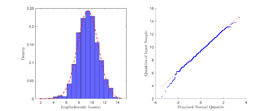
Figure 7.1: Histogram of log-transformed indemnity losses with the fitted normal density (left panel) and the corresponding quantile-quantile plot (right panel).

Table 7.1: Payment-per-payment, $Y$ and payment-per-loss, $Z$ transformation scenarios for the US indemnity losses.

Scenario	Left truncation		Right censorship		$n_{0}$	$n_{1}$	$n_{2}$	$n$	$R$
	LN – $d$	Normal – $t$	LN – $u$	Normal – $T$
Payment $Y$	$500$	$6.2146$	$10^{5}$	$11.5129$	–	1299	152	1451	5.2983
Payment $Z$	$500$	$6.2146$	$10^{5}$	$11.5129$	49	1299	152	1500	5.2983

Note: LN stands for LogNormal, $t=\log{(d-w_{0})}$, and $T=\log{(u-w_{0})}$.

A couple of crucial points are in queue to be mentioned here before starting real data analysis. First, for payment $Y$, the MTM estimators as well as their asymptotic results are based on the assumption of $0\leq a<1-b\leq s^{*}\leq 1$. Initially, we set

$$\hat{s}_{\mbox{\tiny E}}^{*}:=\dfrac{F_{n}(T)-F_{n}(t)}{1-F_{n}(t)}={n_{1}}/{n},\quad\mbox{where $F_{n}$ is the empirical cdf},$$

and choose $b$ such that $1-b\leq\hat{s}_{\mbox{\tiny E}}^{*}$. But after estimating $\widehat{\theta}_{\mbox{\tiny y,MTM}}$ and $\widehat{\sigma}_{\mbox{\tiny y,MTM}}$, it could be the case that

$$\hat{s}_{\mbox{\tiny P}}^{*}:=\dfrac{\widehat{F}_{X}(T)-\widehat{F}_{X}(t)}{1-\widehat{F}_{X}(t)}<1-b,\quad\mbox{where $\widehat{F}_{X}$ is the estimated parametric cdf},$$

which is unsatisfactory for statistical inferences as it violates the assumption (Case 2 from Section 4.1). Therefore, the value of $b$ should be chosen dynamically such that $1-b\leq\min\{\hat{s}_{\mbox{\tiny E}}^{*},\hat{s}_{\mbox{\tiny P}}^{*}\}.$ Similarly, for payment $Z$, the left and right trimming proportions $a$ and $b$, respectively, should be chosen dynamically as:

$$\max\{F_{n}(t),\widehat{F}_{X}(t)\}\leq a\quad\mbox{and}\quad 1-b\leq\min\{F_{n}(T),\widehat{F}_{X}(T)\}.$$

The trimming proportions in Tables 7.2 and 7.3 are chosen accordingly.

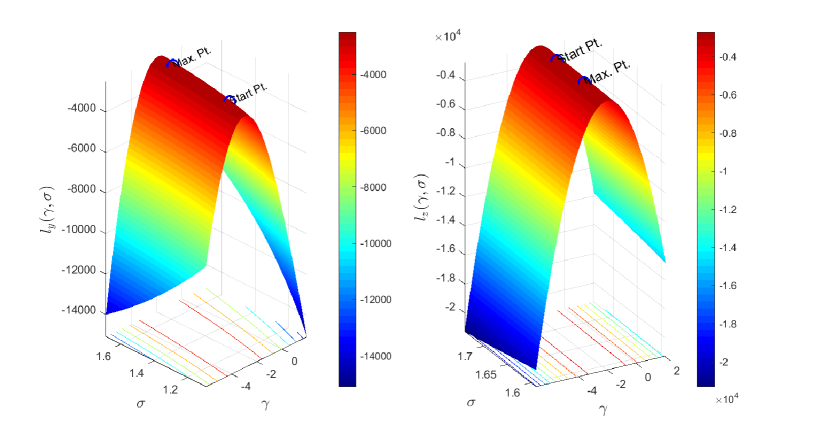
Figure 7.2: Log-likelihood surfaces for payment-per-payment (left panel) and payment-per-loss (right panel) data scenarios given by Equations (3.1) and (3.2), respectively.

For payment-per-payment data scenario, the MLE system of Equations (3.8) takes the form:

$$\left\{\begin{array}[]{rrr}\sigma\left(\Omega_{y,1}-\Omega_{y,2}-\gamma\right)-2.9762&=&0,\\[10.0pt] \sigma^{2}\left(1-\gamma(\Omega_{y,1}-\Omega_{y,2}-\gamma)-\frac{5.2983\Omega_{y,2}}{\sigma}\right)-10.3394&=&0,\end{array}\right.$$ (7.3)

with the first approximations: $(\gamma_{\mbox{\tiny start}},\sigma_{\mbox{\tiny start}})=(-2.4453,1.2171)$, denoted by “Start Pt.” on the corresponding log-likelihood surface given by Figure 7.2 (left panel), but note that $\Omega_{y,1}$ and $\Omega_{y,2}$ also depend on $\gamma$ and $\sigma$. The final MLE solution $\left(\widehat{\gamma}_{\mbox{\tiny y,MLE}},\widehat{\sigma}_{\mbox{\tiny y,MLE}}\right)$ of the system (7.3) is identified with “Max. Pt.” in Figure 7.2 (left panel). Similarly, with different left and right trimming proportions, the system of MTM equations given by (4.15) can be solved with their respective first approximations given by (4.16). The estimated values with their corresponding asymptotic $95\%$ confidence intervals are displayed in Table 7.2. The confidence intervals for $\sigma$ provided are log-transformed confidence intervals (see, e.g., Klugman et al., 2019, p. 315-316) since some of the linear confidence intervals for $\sigma$ include $0$ which are unsatisfactory as $\sigma>0$. For completely observed ground-up lognormal severity data, $\mbox{ARE}\left(\left(\widehat{\theta}_{\mbox{\tiny MTM}},\widehat{\sigma}_{\mbox{\tiny MTM}}\right),\left(\widehat{\theta}_{\mbox{\tiny MLE}},\widehat{\sigma}_{\mbox{\tiny MLE}}\right)\right)$ does not depend on any unknown parameters to be estimated (Brazauskas et al., 2009). But for payment $Y$ and payment $Z$ data scenarios, the corresponding AREs, respectively, given by (4.21) and (4.29) depend on the unknown parameters $\theta$ and $\sigma$. Therefore, for comparison purpose, in Tables 7.2 and 7.3, the $\widehat{\mbox{ARE}}$ column is computed as a bivariate function of MLE estimated values $\widehat{\theta}_{\mbox{\tiny MLE}}$ and $\widehat{\sigma}_{\mbox{\tiny MLE}}$. As seen in Table 7.2, the estimated values of $\theta$ and $\sigma$ via MTM are seem to underestimate the MLE estimated values $\left(\widehat{\theta}_{\mbox{\tiny MLE}},\widehat{\sigma}_{\mbox{\tiny MLE}}\right)=\left(9.43,1.59\right)$ but it is important to note that all the MTM estimated values of $\theta$ and $\sigma$ are close enough to the corresponding MLE estimator even after removing some of the point mass at the right-censored point. It is also noticeable that with trimming pair $(a,b)=(100/1451,300/1451),$ the estimated values of $\theta$ and $\sigma$ are almost equal to the corresponding MLE estimators but still maintaining the efficiency about of 79%. These all demonstrate the robustness of MTM estimators.

Table 7.2: MLE and MTM estimators of $\theta$ and $\sigma$ with their corresponding asymptotic confidence intervals and estimated values of AREs for payment $Y$ data scenario.

Estimators			$\widehat{\theta}$	$\widehat{\sigma}$	$\hat{s}^{*}$		95% CI for		$\widehat{\mbox{ARE}}$	KS Test
					$\hat{s}_{\mbox{\tiny E}}^{*}$	$\hat{s}_{\mbox{\tiny P}}^{*}$	$\theta$	$\sigma$		$D_{y}$	$h_{y}$
MLE			9.43	1.59	–	–	$(9.34,9.52)$	$(1.52,1.67)$	1.00	.032	0
MTM	$a$	$b$	Condition required: $1-b\leq\min\{\hat{s}_{\mbox{\tiny E}}^{*},\hat{s}_{\mbox{\tiny P}}^{*}\}.$
	0.00	150/1451	9.42	1.56	0.90	0.91	$(9.34,9.51)$	$(1.49,1.65)$	0.94	.034	0
	0.00	200/1451	9.42	1.55	0.90	0.91	$(9.33,9.51)$	$(1.47,1.64)$	0.89	.034	0
	0.00	300/1451	9.42	1.54	0.90	0.91	$(9.33,9.50)$	$(1.45,1.63)$	0.80	.034	0
	0.00	700/1451	9.37	1.47	0.90	0.93	$(9.27,9.47)$	$(1.35,1.59)$	0.48	.043	1
	10/1451	150/1451	9.42	1.57	0.90	0.91	$(9.33,9.51)$	$(1.49,1.65)$	0.94	.033	0
	50/1451	200/1451	9.41	1.59	0.90	0.91	$(9.32,9.50)$	$(1.50,1.67)$	0.89	.030	0
	100/1451	300/1451	9.40	1.59	0.90	0.90	$(9.31,9.50)$	$(1.50,1.69)$	0.79	.028	0
	650/1451	650/1451	9.26	2.09	0.90	0.85	$(8.96,9.56)$	$(1.56,2.81)$	0.24	.064	1

Note: For the KS Test column, $D_{y}$ stands for Kolmogorov-Smirnov test statistics and $h_{y}\in\{0,1\}$ stands for the corresponding decision. $h_{y}=0$ means that the assumed model is plausible and $h_{y}=1$ means that the model is rejected.

In order to conduct hypothesis test for the various fitted models, we use the KS test statistic. The KS test statistic for payments $Y$ data set is defined as (see, e.g., Klugman et al., 2019, §15.4.1, p. 360):

$$D_{y} :=\max_{0<y\leq c(u-d)}\left|F_{n}(y)-\widehat{F}_{Y}(y)\right|,$$ (7.4)

where $\widehat{F}_{Y}$ is the estimated cdf given by (2.8). For each fitted model, the corresponding KS test statistics $(D_{y})$ and the decision $(h_{y})$ of the hypothesis test are given in the last two columns of Table 7.2 where $h_{y}=0$ indicates that the lognormal model is plausible and $h_{y}=1$ means that the the lognormal model is rejected at the significance level of $5\%$. Only one model fitted with $(a,b)=\left(650/1451,650/1451\right)\approx(.45,.45)$ is rejected which is close to median-type estimator.

Similarly, for payment-per-loss data scenario, the MLE system of Equations (3.33) takes the form:

$$\left\{\begin{array}[]{rrr}\sigma\left(\Omega_{z,1}-\Omega_{z,2}-\gamma\right)-2.9762&=&0,\\[10.0pt] \sigma^{2}\left(1-\gamma(\Omega_{z,1}-\Omega_{z,2}-\gamma)-\frac{5.2983\Omega_{z,2}}{\sigma}\right)-10.3394&=&0,\end{array}\right.$$ (7.7)

with the first approximations: $(\gamma_{\mbox{\tiny start}},\sigma_{\mbox{\tiny start}})=(-1.8430,1.6998)$. The starting point and the final MLE solution, respectively, are represented by “Start Pt.” and “Max. Pt.” on the log-likelihood surface $l_{z}(\gamma,\sigma)$ given by Figure 7.2 (right panel). Including the corresponding MTM calculation, a summary statistics is displayed in Table 7.3. In this case, as expected all the MTM estimators of $\theta$ are same which clearly demonstrate the stability of the MTM methodology. On the other hand, highly robust MTM estimated value of $\widehat{\sigma}=2.36$ with $(a,b)=(700/1500,700/1500)\approx(.47,.47)$ seems to be more volatile and loosing about 84% of asymptotic efficiency.

Table 7.3: MLE and MTM estimators of $\theta$ and $\sigma$ with their corresponding asymptotic confidence intervals and estimated values of AREs for payment $Z$ data scenario.

Estimators			$\widehat{\theta}$	$\widehat{\sigma}$	$\widehat{F}_{X}(t)$	$\widehat{F}_{X}(T)$	95% CI for		$\small\widehat{\mbox{ARE}}$	KS Test
							$\theta$	$\sigma$		$D_{z}$	$h_{z}$
MLE			9.39	1.64	–	–	$(9.30,9.47)$	$(1.58,1.71)$	1.00	.027	0
MTM	$a$	$b$	Condition required:
			$\max\{F_{n}(t),\widehat{F}_{X}(t)\}\leq a\quad\mbox{and}\quad 1-b\leq\min\{F_{n}(T),\widehat{F}_{X}(T)\}.$
	75/1500	150/1500	9.38	1.62	0.03	0.91	$(9.30,9.47)$	$(1.55,1.69)$	0.92	.027	0
	75/1500	225/1500	9.38	1.61	0.02	0.91	$(9.30,9.47)$	$(1.54,1.69)$	0.86	.027	0
	75/1500	375/1500	9.38	1.60	0.02	0.91	$(9.29,9.46)$	$(1.53,1.69)$	0.76	.027	0
	75/1500	750/1500	9.36	1.59	0.02	0.91	$(9.26,9.47)$	$(1.49,1.70)$	0.52	.028	0
	150/1500	150/1500	9.38	1.63	0.03	0.90	$(9.30,9.47)$	$(1.55,1.70)$	0.86	.026	0
	225/1500	225/1500	9.38	1.63	0.03	0.90	$(9.29,9.46)$	$(1.55,1.72)$	0.76	.026	0
	375/1500	375/1500	9.38	1.61	0.02	0.91	$(9.29,9.47)$	$(1.50,1.71)$	0.57	.027	0
	700/1500	700/1500	9.38	2.36	0.09	0.82	$(9.23,9.52)$	$(1.92,2.91)$	0.16	.107	1

Note: $\left(F_{n}(t),F_{n}(T)\right)=(49/1500,1348/1500)\approx(0.03,0.90).$ For the KS Test column, $D_{z}$ stands for Kolmogorov-Smirnov test statistics and $h_{z}\in\{0,1\}$ stands for the corresponding decision. $h_{z}=0$ means that the assumed model is plausible and $h_{z}=1$ means that the model is rejected.

Further, the KS test statistic for payments $Z$ data set is defined by:

$$D_{z} :=\max_{0\leq z\leq c(u-d)}\left|F_{n}(z)-\widehat{F}_{Z}(z)\right|,$$ (7.8)

where $\widehat{F}_{Z}$ is the estimated parametric cdf given by (2.13). As can be seen in Table 7.3, similar to 7.3, only one model fitted for payment-per-loss data scenario with $(a,b)=(700/1500,700/1500)\approx(.47,.47)$ is rejected with the significance level of $5\%$, but this model is loosing about 84% of the ARE compared to the corresponding MLE model.

In conclusion, a take-home knowledge from Tables 7.2 and 7.3 is that since the sample data is already either truncated and/or censored, then a robust estimation procedure still maintaining high relative efficiency with respect to the corresponding MLE is simply to eliminate the point masses at the truncated and censored values. For example, $MTM(a=0,b=150/1451)$ and $MTM(a=10/1451,b=150/1451)$ from Table 7.2 and $MTM(a=75/1500,b=150/1500)$ from Table 7.3.

8 Summary and Future Direction

In this paper, we have developed two estimation procedures – maximum likelihood and a dynamic MTM for lognormal insurance payment-per-payment and payment-per-loss loss severity data. A series of theoretical results about estimators’ existence and asymptotic normality are established. As seen in Tables 4.1 and 4.2, the dynamic MTM estimators sacrifice little asymptotic efficiency with respect to MLE but are more robust as well as computationally more efficient than MLE if properly implemented, see, for example, (4.28) and Note 4.1, and these properties are highly desirable in practice. Finally, the developed estimators are implemented on a real-life data set to analyze the 1500 US indemnity losses which is widely studied in the actuarial literature (see, e.g., Frees and Valdez, 1998, Michael et al., 2020), and it is found that most of the fitted models are plausible for this data set.

The results of this paper motivate open problems and generate several ideas for further research. First, this paper is specifically focused on lognormal insurance payment severity models, but they could be extended to more general (log) location-scale and exponential dispersion families. Second, several contaminated loss severity models are proposed in the literature as mentioned in Section 1 Introduction, so it could even produce a better model still maintaining a reasonable balance between efficiency and robustness if one implements the dynamic MTM procedures for those mixture models, but it is recommended to design the MTM for the complete mixture models first. Third, in this paper we only discussed about model-fitting procedures and the corresponding finite sample performance, but the ultimate goal of model fitting is to apply the fitted models in decision-making mechanism. Therefore, it is yet to measure how the estimators developed in this paper act in calculating actuarial pure premium as well as in different risk analysis in practice.

Finally, it is important to emphasize again that the motivation to implement the MTM approach rather than MLE even for truncated and/or censored loss data sets is to simultaneously remove partial point masses assigned by MLE at the truncated and/or censored data points (that is, achieving a desired degree of robustness) and maintaining a high degree of ARE, too. Further, the dynamic MTM procedures designed in this paper can only be implemented if a close fit in one or both tails of the assumed underlying distribution is not desired, otherwise extreme value modeling is recommended.

Appendix A Auxiliary Results

Define $\bar{a}:=1-a$, $\bar{b}:=1-b$, and $\tau:=1-a-b$.

1. The expressions for $c_{k},\ 1\leq k\leq 4$ mentioned in Section 4.2 are given by

   $$c_{k} \equiv c_{k}(\Phi,a,b)=\dfrac{1}{\tau}\int_{a}^{\bar{b}}\left[\Phi^{-1}(s)\right]^{k}\,ds.$$

2. The expressions for $c_{k}^{*},\ 1\leq k\leq 3$ used in Section 4.2 are given as below:

   $$c_{1}^{*} =\left(\dfrac{1}{\tau}\right)^{2}\int_{a}^{\bar{b}}\int_{a}^{\bar{b}}{\frac{\min\>\{u,v\}-uv}{\phi\left[\Phi^{-1}\left(v\right)\right]\phi\left[\Phi^{-1}\left(u\right)\right]}}\,dv\,du$$

   $$=\left(\dfrac{1}{\tau}\right)^{2}\left\{a\bar{a}\left[\Phi^{-1}(a)\right]^{2}+b\bar{b}\left[\Phi^{-1}(\bar{b})\right]^{2}-2ab\Phi^{-1}(a)\Phi^{-1}(\bar{b})\right.$$

   $$\quad\left.-2\tau c_{1}\left[a\Phi^{-1}(a)+b\Phi^{-1}(\bar{b})\right]-\tau^{2}c_{1}^{2}+\tau c_{2}\right\}.$$

   $$c_{2}^{*} =\left(\dfrac{1}{\tau}\right)^{2}\int_{a}^{\bar{b}}\int_{a}^{\bar{b}}{\frac{\left(\min\>\{u,v\}-uv\right)\Phi^{-1}(u)}{\phi\left[\Phi^{-1}\left(v\right)\right]\phi\left[\Phi^{-1}\left(u\right)\right]}}\,dv\,du$$

   $$=\dfrac{1}{2\tau^{2}}\left\{a\bar{a}\left[\Phi^{-1}(a)\right]^{3}+b\bar{b}\left[\Phi^{-1}(\bar{b})\right]^{3}-ab\Phi^{-1}(a)\Phi^{-1}(\bar{b})\left[\Phi^{-1}(a)+\Phi^{-1}(\bar{b})\right]\right.$$

   $$\quad\left.-\tau c_{1}\left[a\left[\Phi^{-1}(a)\right]^{2}+b\left[\Phi^{-1}(\bar{b})\right]^{2}\right]-\tau c_{2}\left[a\Phi^{-1}(a)+b\Phi^{-1}(\bar{b})\right]-\tau^{2}c_{1}c_{2}+\tau c_{3}\right\}.$$

   $$c_{3}^{*} =\left(\dfrac{1}{\tau}\right)^{2}\int_{a}^{\bar{b}}\int_{a}^{\bar{b}}{\frac{\left(\min\>\{u,v\}-uv\right)\Phi^{-1}(v)\Phi^{-1}(u)}{\phi\left[\Phi^{-1}\left(v\right)\right]\phi\left[\Phi^{-1}\left(u\right)\right]}}\,dv\,du$$

   $$=\dfrac{1}{4\tau^{2}}\left\{a\bar{a}\left[\Phi^{-1}(a)\right]^{4}+b\bar{b}\left[\Phi^{-1}(\bar{b})\right]^{4}-2ab\left[\Phi^{-1}(a)\right]^{2}\left[\Phi^{-1}(\bar{b})\right]^{2}\right.$$

   $$\quad\left.-2\tau c_{2}\left[a\left[\Phi^{-1}(a)\right]^{2}+b\left[\Phi^{-1}(\bar{b})\right]^{2}\right]-\tau^{2}c_{2}^{2}+\tau c_{4}\right\}.$$

3. The entries of the variance-covariance matrix $\bm{\Sigma}_{y}$ from Section 4.1 are as follows:

   $$c_{y,1}^{*} =\left(\frac{\bar{\Phi}(\gamma)}{\tau}\right)^{2}\int_{a}^{\bar{b}}\int_{a}^{\bar{b}}{\frac{\text{min}\>\{u,v\}-uv}{\phi\left[\Phi^{-1}\left(v+(1-v)\Phi(\gamma)\right)\right]\phi\left[\Phi^{-1}\left(u+(1-u)\Phi(\gamma)\right)\right]}}\,dv\,du.$$

   $$c_{y,2}^{*} =\left(\frac{\bar{\Phi}(\gamma)}{\tau}\right)^{2}\int_{a}^{\bar{b}}\int_{a}^{\bar{b}}{\frac{\left[\text{min}\>\{u,v\}-uv\right]\Phi^{-1}\left(u+(1-u)\Phi(\gamma)\right)}{\phi\left[\Phi^{-1}\left(v+(1-v)\Phi(\gamma)\right)\right]\phi\left[\Phi^{-1}\left(u+(1-u)\Phi(\gamma)\right)\right]}}\,dv\,du.$$

   $$c_{y,3}^{*} =\left(\frac{\bar{\Phi}(\gamma)}{\tau}\right)^{2}\int_{a}^{\bar{b}}\int_{a}^{\bar{b}}\left[{\frac{\left[\text{min}\>\{u,v\}-uv\right]\Phi^{-1}\left(v+(1-v)\Phi(\gamma)\right)}{\phi\left[\Phi^{-1}\left(v+(1-v)\Phi(\gamma)\right)\right]}}\right.$$

   $${\qquad\qquad\qquad\qquad\qquad\qquad\qquad\qquad}\times\left.{\frac{\Phi^{-1}\left(u+(1-u)\Phi(\gamma)\right)}{\phi\left[\Phi^{-1}\left(u+(1-u)\Phi(\gamma)\right)\right]}}\right]\,dv\,du.$$

References

- Abu Bakar et al. (2015) Abu Bakar, S. A., Hamzah, N. A., Maghsoudi, M., and Nadarajah, S. (2015). Modeling loss data using composite models. Insurance: Mathematics & Economics, 61:146–154.
- Barrow and Cohen (1954) Barrow, D. F. and Cohen, Jr., A. C. (1954). On some functions involving Mill’s ratio. Annals of Mathematical Statistics, 25:405–408.
- Blostein and Miljkovic (2019) Blostein, M. and Miljkovic, T. (2019). On modeling left-truncated loss data using mixtures of distributions. Insurance: Mathematics & Economics, 85:35–46.
- Brazauskas et al. (2009) Brazauskas, V., Jones, B. L., and Zitikis, R. (2009). Robust fitting of claim severity distributions and the method of trimmed moments. Journal of Statistical Planning and Inference, 139(6):2028–2043.
- Brazauskas and Kleefeld (2016) Brazauskas, V. and Kleefeld, A. (2016). Modeling severity and measuring tail risk of Norwegian fire claims. North American Actuarial Journal, 20(1):1–16.
- Brazauskas and Serfling (2000) Brazauskas, V. and Serfling, R. (2000). Robust and efficient estimation of the tail index of a single-parameter Pareto distribution. North American Actuarial Journal, 4(4):12–27.
- Chan et al. (2018) Chan, J. S. K., Choy, S. T. B., Makov, U. E., and Landsman, Z. (2018). Modelling insurance losses using contaminated generalized beta type-II distribution. ASTIN Bulletin, 48(2):871–904.
- Chernoff et al. (1967) Chernoff, H., Gastwirth, J. L., and Johns, Jr., M. V. (1967). Asymptotic distribution of linear combinations of functions of order statistics with applications to estimation. Annals of Mathematical Statistics, 38(1):52–72.
- Cohen (1950) Cohen, Jr., A. C. (1950). Estimating the mean and variance of normal populations from singly truncated and doubly truncated samples. Annals of Mathematical Statistics, 21(4):557–569.
- Cohen (1951) Cohen, Jr., A. C. (1951). On estimating the mean and variance of singly truncated normal frequency distributions from the first three sample moments. Annals of the Institute of Statistical Mathematics, 3:37–44.
- Cooray and Ananda (2005) Cooray, K. and Ananda, M. M. A. (2005). Modeling actuarial data with a composite lognormal-Pareto model. Scandinavian Actuarial Journal, 2005(5):321–334.
- Ergashev et al. (2016) Ergashev, B., Pavlikov, K., Uryasev, S., and Sekeris, E. (2016). Estimation of truncated data samples in operational risk modeling. The Journal of Risk and Insurance, 83(3):613–640.
- Frees and Valdez (1998) Frees, E. W. and Valdez, E. A. (1998). Understanding relationships using copulas. North American Actuarial Journal, 2(1):1–25.
- Grün and Miljkovic (2019) Grün, B. and Miljkovic, T. (2019). Extending composite loss models using a general framework of advanced computational tools. Scandinavian Actuarial Journal, 2019(8):642–660.
- Gui et al. (2021) Gui, W., Huang, R., and Lin, X. S. (2021). Fitting multivariate Erlang mixtures to data: a roughness penalty approach. Journal of Computational and Applied Mathematics, 386:113216, 17.
- Hampel (1974) Hampel, F. R. (1974). The influence curve and its role in robust estimation. Journal of the American Statistical Association, 69:383–393.
- Hewitt et al. (1979) Hewitt, C. C., Jr., and Lefkowitz, B. (1979). Methods for fitting distributions to insurance loss data. In Proceedings of the Casualty Actuarial Society, volume LXVI, pages 139–160. Casualty Actuarial Society, VA.
- Huber (1964) Huber, P. J. (1964). Robust estimation of a location parameter. Annals of Mathematical Statistics, 35(1):73–101.
- Huber and Ronchetti (2009) Huber, P. J. and Ronchetti, E. M. (2009). Robust Statistics. John Wiley & Sons, Inc., Hoboken, NJ, second edition.
- Klugman et al. (2019) Klugman, S. A., Panjer, H. H., and Willmot, G. E. (2019). Loss Models: From Data to Decisions. John Wiley & Sons, Hoboken, NJ, fifth edition.
- Michael et al. (2020) Michael, S., Miljkovic, T., and Melnykov, V. (2020). Mixture modeling of insurance loss data with multiple level partial censoring. Advances in Data Analysis and Classification, 14:355–378.
- Miljkovic and Grün (2016) Miljkovic, T. and Grün, B. (2016). Modeling loss data using mixtures of distributions. Insurance: Mathematics & Economics, 70:387–396.
- Poudyal (2018) Poudyal, C. (2018). Robust Estimation of Parametric Models for Insurance Loss Data. ProQuest LLC, Ann Arbor, MI. Thesis (Ph.D.)–The University of Wisconsin - Milwaukee.
- Poudyal (2021) Poudyal, C. (2021). Truncated, censored, and actuarial payment-type moments for robust fitting of a single-parameter Pareto distribution. Journal of Computational and Applied Mathematics, 388:113310, 18.
- Punzo et al. (2018) Punzo, A., Bagnato, L., and Maruotti, A. (2018). Compound unimodal distributions for insurance losses. Insurance: Mathematics & Economics, 81:95–107.
- Reynkens et al. (2017) Reynkens, T., Verbelen, R., Beirlant, J., and Antonio, K. (2017). Modelling censored losses using splicing: a global fit strategy with mixed Erlang and extreme value distributions. Insurance: Mathematics & Economics, 77:65–77.
- Scollnik (2007) Scollnik, D. P. M. (2007). On composite lognormal-Pareto models. Scandinavian Actuarial Journal, 2007(1):20–33.
- Scollnik and Sun (2012) Scollnik, D. P. M. and Sun, C. (2012). Modeling with Weibull-Pareto models. North American Actuarial Journal, 16(2):260–272.
- Serfling (2002) Serfling, R. (2002). Efficient and robust fitting of lognormal distributions. North American Actuarial Journal, 6(4):95–109.
- Serfling (1980) Serfling, R. J. (1980). Approximation Theorems of Mathematical Statistics. John Wiley & Sons, New York.
- Shah and Jaiswal (1966) Shah, S. M. and Jaiswal, M. C. (1966). Estimation of parameters of doubly truncated normal distribution from first four sample moments. Annals of the Institute of Statistical Mathematics, 18:107–111.
- Tukey (1960) Tukey, J. W. (1960). A survey of sampling from contaminated distributions. In Contributions to Probability and Statistics, pages 448–485. Stanford University Press, Stanford, CA.
- van der Vaart (1998) van der Vaart, A. W. (1998). Asymptotic Statistics. Cambridge University Press, Cambridge.
- Verbelen et al. (2015) Verbelen, R., Gong, L., Antonio, K., Badescu, A., and Lin, S. (2015). Fitting mixtures of Erlangs to censored and truncated data using the EM algorithm. ASTIN Bulletin, 45(3):729–758.
- Zhao et al. (2018) Zhao, Q., Brazauskas, V., and Ghorai, J. (2018). Robust and efficient fitting of severity models and the method of Winsorized moments. ASTIN Bulletin, 48(1):275–309.