Computing Sum of Sources over a Classical-Quantum MAC

Touheed Anwar Atif1, Arun Padakandla2 and S. Sandeep Pradhan1
Department of Electrical Engineering and Computer Science,
1University of Michigan, Ann Arbor, USA.
2University of Tennessee, Knoxville, USA
Email: touheed@umich.edu, arunpr@utk.edu, pradhanv@umich.edu
Abstract

We consider the problem of communicating a general bivariate function of two classical sources observed at the encoders of a classical-quantum multiple access channel. Building on the techniques developed for the case of a classical channel, we propose and analyze a coding scheme based on coset codes. The proposed technique enables the decoder recover the desired function without recovering the sources themselves. We derive a new set of sufficient conditions that are weaker than the current known for identified examples. This work is based on a new ensemble of coset codes that are proven to achieve the capacity of a classical-quantum point-to-point channel.

I Introduction

Early research in quantum state discrimination led to the investigation of the information carrying capacity of quantum states. Suppose Alice - a sender - can prepare any one of the states in the collection $\{\rho_{x}\in\mathcal{D}(\mathcal{H}_{Y}):x\in\mathcal{X}\}$ and Bob - the receiver - has to rely on a measurement to infer the label $x$ of the state, then what is the largest sub-collection $\mathcal{C}\subseteq\mathcal{X}$ of states that Bob can distinguish perfectly? Studying this question in a Shannon-theoretic sense, Schumacher, Westmoreland [1] and Holevo [2] characterized the exponential growth of this sub-collection, thereby characterizing the capacity of a classical-quantum (CQ) point-to-point (PTP) channel. In the following years, generalizations of this question with multiple senders and/or receivers have been studied with an aim of characterizing the corresponding information carrying capacity of quantum states in network scenarios [3].

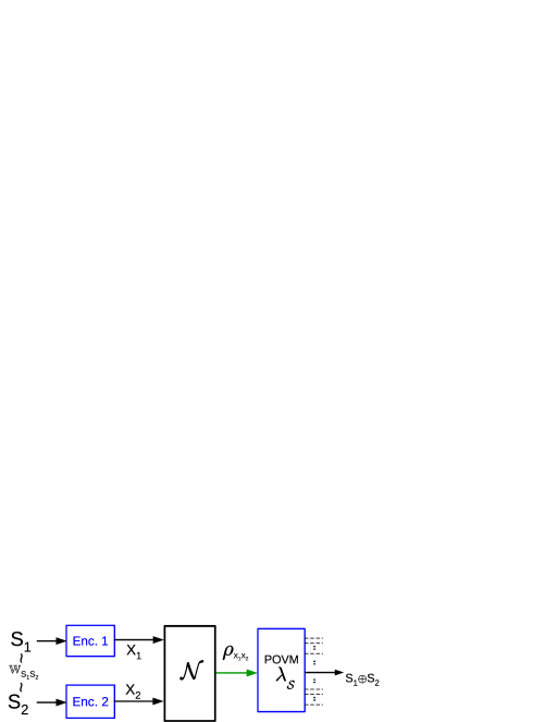
In this work, we consider the problem of computing functions of information sources over a CQ multiple access channel (MAC). Let $(\rho_{x_{1}x_{2}}\in\mathcal{D}(\mathcal{H}_{Y}):(x_{1},x_{2})\in\mathcal{X}_{1}\times\mathcal{X}_{2})$ model a CQ-MAC. Sender $j$ - the party having access to the choice of label $x_{j}\in\mathcal{X}_{j}$ - observes a classical information stream $S_{jt}\in\mathcal{S}_{j}:t\geq 1$. The pairs $(S_{1t},S_{2t}):t\geq 1$ are independent and identically distributed (IID) with a single-letter joint distribution $\mathbb{W}_{S_{1}S_{2}}$. The receiver, who is provided with the prepared quantum state, intends to reconstruct a specific function $f(S_{1},S_{2})$ of the information observed by the senders. The question of interest is under what conditions, specified in terms of the CQ-MAC, $\mathbb{W}_{S_{1}S_{2}}$ and $f$, can the receiver reconstruct the desired function losslessly?

The conventional approach to characterizing sufficient conditions for this problem relies on enabling the receiver reconstruct the pair of classical source sequences. Since the receiver is only interested in recovering the bivariate function $f$, and not the pair, this approach can be strictly sub-optimal. Can we exploit this and design a more efficient communication strategy, thereby weakening the set of sufficient conditions? In this work, we present one such communication strategy for a general CQ-MAC that is more efficient than the conventional approach. This strategy is based on asymptotically good random nested coset codes. We analyze its performance and derive new sufficient conditions for a general problem instance and identify examples for which the derived conditions are strictly weaker.

Refer to caption
Figure 1: CQ-MAC used for computing sum of classical sources.

Our findings here are built on the ideas developed in the classical setting. Focusing on a source coding formulation, i.e. a noiseless MAC, Kรถrner and Marton [4] devised an ingenious coding technique that enabled the receiver recover the sum of the sources without recovering either source. In [5], the linearity of the Kรถrner-Marton (KM) source coding map was further exploited to enable the receiver recover the sum of the sources using only the sum of the KM indices, not even requiring the pair. Leveraging this observation and focusing on the subclass of additive MACs, specific MAC channel coding techniques are devised in [5] that enabled the receiver recover the sum of two channel coding message indices.

The techniques of [4], [5] are instances of a broader framework of coding strategies. Decoding functions of sources or channel inputs efficiently require codes endowed with algebraic closure properties. To emphasize, the conventional approach of deriving inner bounds/achievable rate region by analyzing expected performance of IID random codes is incapable of yielding performance limits - capacity or rate-distortion regions as the case may be- in network communication scenarios. To improve upon this, it is necessary to analyze the expected performance of random codes endowed with algebraic closure properties. In a series of works [6], an information theoretic study of the latter codes has been carried out yielding new inner bounds for multiple network communication scenarios.

In this work, we embark on developing these ideas in the CQ setup. After having provided the problem statement in Sec.ย II, we focus on a simplified CQ MAC and illustrate the core idea of our coding scheme. The latter relies on developing a nested coset code (NCC) based communication scheme for a CQ PTP channel and analyzing its performance (Sec.ย IV). Leveraging this building block, we design and analyze the performance of an NCC-based coding scheme for computing sum over a general CQ-MAC (Sec.ย VI). Going further we generalize this idea for computing arbitrary functions over a general CQ-MAC.

II Preliminaries and Problem Statement

We supplement the notation in [7] with the following. For positive integer $n$, $[n]\mathrel{\ensurestackMath{\stackon[1pt]{=}{\scriptstyle\Delta}}}\left\{1,\cdots,n\right\}$. For a Hilbert space $\mathcal{H}$, $\mathcal{L}(\mathcal{H}),\mathcal{P}(\mathcal{H})$ and $\mathcal{D}(\mathcal{H})$ denote the collection of linear, positive and density operators acting on $\mathcal{H}$, respectively. The von Neumann entropy of a density operator $\rho\in\mathcal{D}(\mathcal{H})$ is denoted by $S(\rho)$. Given any ensemble $\{p_{i},\rho_{i}\}_{i\in[1,m]}$, the Holevo information [8] is denoted as $\chi\big{(}\{p_{i};\rho_{i}\}\big{)}$. A POVM acting on $\mathcal{H}$ is a collection $\lambda_{\mathcal{X}}\mathrel{\ensurestackMath{\stackon[1pt]{=}{\scriptstyle\Delta}}}\{\lambda_{x}\}_{x\in\mathcal{X}}$ of positive operators that form a resolution of the identity: $\sum_{x\in\mathcal{X}}\lambda_{x}=I$, where $\mathcal{X}$ is a finite set. We employ an underline notation to aggregate objects of similar type. For example, sยฏยฏ๐‘ \underline{s} denotes (s1,s2)subscript๐‘ 1subscript๐‘ 2(s_{1},s_{2}), $\underline{x}^{n}$ denotes $(x_{1}^{n},x_{2}^{n})$, $\underline{\mathcal{S}}$ denotes the Cartesian product $\mathcal{S}_{1}\times\mathcal{S}_{2}$.

Consider a (generic) CQ-MAC $(\rho_{x_{1}x_{2}}\in\mathcal{D}(\mathcal{H}_{Y}):(x_{1},x_{2})\in\mathcal{X}_{1}\times\mathcal{X}_{2})$ specified through (i) finite sets $\mathcal{X}_{j}:j\in[2]$, (ii) Hilbert space $\mathcal{H}_{Y}$, and (iii) a collection $(\rho_{x_{1},x_{2}}\in\mathcal{D}(\mathcal{H}_{Y}):(x_{1},x_{2})\in\mathcal{X}_{1}\times\mathcal{X}_{2})$ of density operators. This CQ-MAC is employed to enable the receiver reconstruct a bivariate function of the classical information streams observed by the senders. Let $\mathcal{S}_{1},\mathcal{S}_{2}$ be finite sets and $(S_{1},S_{2})\in\mathcal{S}_{1}\times\mathcal{S}_{2}$ distributed with PMF $\mathbb{W}_{S_{1}S_{2}}$ models the pair of information sources observed at the encoders. Specifically, sender $j$ observes the sequence $S_{jt}\in\mathcal{S}_{j}:t\geq 1$ and the sequence $(S_{1t},S_{2t}):t\geq 1$ are IID with single-letter PMF $\mathbb{W}_{S_{1}S_{2}}$. The receiver aims to recover the sequence $f(S_{1t},S_{2t}):t\geq 1$ losslessly, where $f:\mathcal{S}_{1}\times\mathcal{S}_{2}\rightarrow\mathcal{R}$ is a specified function.

A CQ-MAC code $c_{f}=(n,e_{1},e_{2},\lambda_{\mathcal{R}^{n}})$ of block-length $n$ for recovering $f$ consists of two encoders maps $e_{j}:\mathcal{S}^{n}\rightarrow\mathcal{X}_{j}^{n}:j\in[2]$, and a POVM $\lambda_{\mathcal{R}^{n}}=\{\lambda_{r^{n}}\in\mathcal{P}(\mathcal{H}_{Y}^{\otimes n}):r^{n}\in\mathcal{R}^{n}\}$. The average error probability of the CQ-MAC code $c_{f}$ is

$\displaystyle\overline{\xi}(c_{f})$ $\displaystyle=$ 1โˆ’โˆ‘sยฏn:fโ€‹(sยฏn)=rn๐•ŽS1โ€‹S2nโ€‹(s1n,s2n)โ€‹trโก(ฮปrnโ€‹ฯc,sยฏnโŠ—n)1subscript:superscriptยฏ๐‘ ๐‘›๐‘“superscriptยฏ๐‘ ๐‘›superscript๐‘Ÿ๐‘›superscriptsubscript๐•Žsubscript๐‘†1subscript๐‘†2๐‘›superscriptsubscript๐‘ 1๐‘›superscriptsubscript๐‘ 2๐‘›tracesubscript๐œ†superscript๐‘Ÿ๐‘›subscriptsuperscript๐œŒtensor-productabsent๐‘›๐‘superscriptยฏ๐‘ ๐‘›\displaystyle 1-\sum_{\underline{s}^{n}:f(\underline{s}^{n})=r^{n}}\mathbb{W}_{S_{1}S_{2}}^{n}(s_{1}^{n},s_{2}^{n})\tr(\lambda_{r^{n}}\rho^{\otimes n}_{c,\underline{s}^{n}})

where $\rho^{\otimes n}_{c,\underline{s}^{n}}\mathrel{\ensurestackMath{\stackon[1pt]{=}{\scriptstyle\Delta}}}\otimes_{i=1}^{n}\rho_{x_{1i}(s_{1}^{n})x_{2i}(s_{2}^{n})}$, where ejโ€‹(sjn)=xjโ€‹1โ€‹(sjn),xjโ€‹2โ€‹(sjn),โ‹ฏ,xjโ€‹nโ€‹(sjn)subscript๐‘’๐‘—superscriptsubscript๐‘ ๐‘—๐‘›subscript๐‘ฅ๐‘—1superscriptsubscript๐‘ ๐‘—๐‘›subscript๐‘ฅ๐‘—2superscriptsubscript๐‘ ๐‘—๐‘›โ‹ฏsubscript๐‘ฅ๐‘—๐‘›superscriptsubscript๐‘ ๐‘—๐‘›e_{j}(s_{j}^{n})=x_{j1}(s_{j}^{n}),x_{j2}(s_{j}^{n}),\cdots,x_{jn}(s_{j}^{n}) for $j\in[2]$.

A function $f$ of the sources $\mathbb{W}_{S_{1}S_{2}}$ is said to be reconstructible over a CQ-MAC if for $\epsilon>0$, $\exists$ a sequence $c_{f}^{(n)}=(n,e_{1}^{(n)},e_{2}^{(n)},\lambda_{\mathcal{R}^{n}}):n\geq 1$ such that $\lim_{n\rightarrow\infty}\overline{\xi}(c_{f}^{(n)})=0$.

In this article, we are concerned with the problem of characterizing sufficient conditions under which a function $f$ of the sources $\mathbb{W}_{S_{1}S_{2}}$ is reconstructible over a generic MAC $(\rho_{x_{1}x_{2}}\in\mathcal{D}(\mathcal{H}_{Y}):(x_{1},x_{2})\in\mathcal{X}_{1}\times\mathcal{X}_{2})$. One of our findings - Proposition 2 - provides a characterization of sufficient conditions in terms of a computable function of the associated objects- density operators that characterize the CQ-MAC, function $f$ and the source distribution $\mathbb{W}_{S_{1}S_{2}}$.

As we shall see, the specific problem of computing sum of sources will play an important role in our work. In this case, $\mathcal{S}=\mathcal{S}_{1}=\mathcal{S}_{2}=\mathcal{F}_{q}$ is a finite field with $q$ elements and the receiver aims to reconstruct $f(S_{1},S_{2})=S_{1}\oplus_{q}S_{2}$ where $\oplus_{q}$ denotes addition in $\mathcal{F}_{q}$. A CQ-MAC code $c_{\oplus}=(n,e_{1},e_{2},\lambda_{\mathcal{S}^{n}})$ of block-length $n$ for recovering the sum consists of two encoders maps $e_{j}:\mathcal{S}^{n}\rightarrow\mathcal{X}_{j}^{n}:j\in[2]$, and a POVM ฮป๐’ฎn={ฮปsnโˆˆ๐’ซโ€‹(โ„‹YโŠ—n):snโˆˆ๐’ฎn}subscript๐œ†superscript๐’ฎ๐‘›conditional-setsubscript๐œ†superscript๐‘ ๐‘›๐’ซsuperscriptsubscriptโ„‹๐‘Œtensor-productabsent๐‘›superscript๐‘ ๐‘›superscript๐’ฎ๐‘›\lambda_{\mathcal{S}^{n}}=\{\lambda_{s^{n}}\in\mathcal{P}(\mathcal{H}_{Y}^{\otimes n}):s^{n}\in\mathcal{S}^{n}\}.

Restricting $f$ to a sum, we say the sum of sources $\mathbb{W}_{S_{1}S_{2}}$ over field $\mathcal{F}_{q}$ is reconstructible over a CQ-MAC if $\mathcal{S}_{1}=\mathcal{S}_{2}=\mathcal{F}_{q}$ and the function $f(S_{1},S_{2})=S_{1}\oplus_{q}S_{2}$ is reconstructible over the CQ-MAC. The problem of characterizing sufficient conditions under which a sum of sources is reconstructible over a CQ-MAC plays an important role in this work. One of our findings - Theorem 2 - provides a computable characterization of a set of sufficient conditions under which a sum of sources is reconstructible over a CQ-MAC. As the reader will note, this encapsulates the central element of our characterization in Proposition 2.

We also formalize the notions of a CQ-PTP and CQ-MAC codes for communicating uniform messages. A CQ-MAC code $c_{\underline{m}}=(n,\mathcal{I}_{1},\mathcal{I}_{2},e_{1},e_{2},\lambda_{\underline{\mathcal{I}}})$ for a CQ-MAC $(\rho_{\underline{x}}\in\mathcal{D}(\mathcal{H}_{Y}):\underline{x}\in\underline{\mathcal{X}})$ consists of (i) index sets $\mathcal{I}_{j}:j\in[2]$, (ii) encoder maps $e_{j}:\mathcal{I}_{j}\rightarrow\mathcal{X}_{j}^{n}:j\in[2]$ and a decoding POVM $\lambda_{\underline{\mathcal{I}}}=\{\lambda_{\underline{m}}\in\mathcal{P}(\mathcal{H}_{Y}^{\otimes n}):\underline{m}\in\mathcal{I}_{1}\times\mathcal{I}_{2}\}$. For $\underline{m}\in\mathcal{I}_{1}\times\mathcal{I}_{2}$, we let $\rho^{\otimes n}_{c,\underline{m}}\mathrel{\ensurestackMath{\stackon[1pt]{=}{\scriptstyle\Delta}}}\otimes_{i=1}^{n}\rho_{x_{1i},x_{2i}}$ where $e_{j}(m_{j})=x_{j1}\cdots x_{jn}$ for $j\in[2]$.

A CQ-PTP code $c_{m}=(n,\mathcal{I},e,\lambda_{\mathcal{I}})$ for a CQ-PTP $(\rho_{x}\in\mathcal{D}(\mathcal{H}_{Y}):x\in\mathcal{X})$ consists of (i) an index set $\mathcal{I}$, (ii) and encoder map $e:\mathcal{I}\rightarrow\mathcal{X}^{n}$ and a decoding POVM $\lambda_{\mathcal{I}}=\{\lambda_{m}\in\mathcal{P}(\mathcal{H}_{Y}^{\otimes n}):m\in\mathcal{I}\}$. For $m\in\mathcal{I}$, we let $\rho_{c,m}^{\otimes n}\mathrel{\ensurestackMath{\stackon[1pt]{=}{\scriptstyle\Delta}}}\otimes_{i=1}^{n}\rho_{x_{i}}$ where $e(m)=x_{1}\cdots x_{n}$.

III The Central Idea

Let us consider the specific problem of reconstructing the sum of sources each taking values in $\mathcal{S}=\mathcal{F}_{q}$. We begin by reviewing the KM coding scheme for the case of a noiseless classical MAC. It was shown in [4] the existence of linear code with a parity matrix $H\in\mathcal{S}^{l\times n}$ and decoder map $d:\mathcal{F}_{q}^{l}\rightarrow\mathcal{S}^{n}$ such that โˆ‘sยฏnโˆˆ๐’ฎยฏn๐•ŽSยฏnโ€‹(sยฏn)โ€‹๐Ÿ™{dโ€‹(Hโ€‹s1nโŠ•qHโ€‹s2n)โ‰ s1nโŠ•qs2n}โ‰คฯตsubscriptsuperscriptยฏ๐‘ ๐‘›superscriptยฏ๐’ฎ๐‘›superscriptsubscript๐•Žยฏ๐‘†๐‘›superscriptยฏ๐‘ ๐‘›subscript1๐‘‘subscriptdirect-sum๐‘ž๐ปsuperscriptsubscript๐‘ 1๐‘›๐ปsuperscriptsubscript๐‘ 2๐‘›subscriptdirect-sum๐‘žsuperscriptsubscript๐‘ 1๐‘›superscriptsubscript๐‘ 2๐‘›italic-ฯต\sum_{\underline{s}^{n}\in\underline{\mathcal{S}}^{n}}\mathbb{W}_{\underline{S}}^{n}(\underline{s}^{n})\mathds{1}_{\{d(Hs_{1}^{n}\oplus_{q}Hs_{2}^{n})\neq s_{1}^{n}\oplus_{q}s_{2}^{n}\}}\leq\epsilon, for any $\epsilon>0$, and sufficiently large $n$, so long as $\frac{l\log_{2}q}{n}>H(S_{1}\oplus_{q}S_{2})$. This implies that a receiver equipped with the decoding map $d$ can recover the sum if it possesses the sum $M_{1}^{l}\oplus_{q}M_{2}^{l}$ of the Kรถrner-Marton indices $M_{j}^{l}=HS_{j}^{l}:j\in[2]$.

We are therefore led to building an efficient CQ-MAC coding scheme that enables the receiver only reconstruct the sum of the two message indices. Indeed, if the two senders send the KM indices to such a CQ-MAC channel code and the receiver employs the above source decoder $d$ on the decoded sum of the KM indices, it can recover the sum of sources. To illustrate the design of the desired CQ-MAC channel code, let us consider a CQ-MAC $(\rho_{x_{1}x_{2}}\in\mathcal{D}(\mathcal{H}_{Y}):(x_{1},x_{2})\in\mathcal{X}_{1}\times\mathcal{X}_{2})$ wherein $\mathcal{X}_{1}=\mathcal{X}_{2}=\mathcal{F}_{q}$ and the collection $\rho_{\underline{x}}:\underline{x}\in\underline{\mathcal{X}}$ satisfies $\rho_{x_{1}x_{2}}=\rho_{\hat{x}_{1}\hat{x}_{2}}$ whenever $x_{1}\oplus_{q}x_{2}=\hat{x}_{1}\oplus_{q}\hat{x}_{2}$. Consider a CQ-PTP $(\mathcal{X}=\mathcal{F}_{q},\sigma_{u}:u\in\mathcal{X})$ where $\sigma_{u}=\rho_{x_{1}\oplus x_{2}}$ for any $(x_{1},x_{2})$ satisfying $x_{1}\oplus_{q}x_{2}=u$. Suppose we are able to communicate over this CQ-PTP via a linear CQ-PTP code $\mathcal{C}\subseteq\mathcal{X}^{n}$. Specifically, suppose there exists a generator matrix $G\in\mathcal{X}^{l\times n}$ and a POVM $\{\lambda_{m^{l}}:m^{l}\in\mathcal{F}_{q}^{l}\}$ so that $1-q^{-l}\sum_{m^{l}}\tr(\lambda_{m^{l}}\sigma^{\otimes n}_{m^{l}G})\leq\epsilon$. for any $\epsilon>0$ and sufficiently large $n$, where $\sigma^{\otimes}_{m^{l}G}=\sigma_{x_{1}}\otimes\cdots\otimes\sigma_{x_{n}}$ where $m^{l}G=x^{n}$. We can then use this linear CQ-PTP code as our desired CQ-MAC channel code. Indeed, observe that, suppose both senders employ this same linear CQ-PTP code, then sender $j$ maps its KM index mjl=Hโ€‹sjnsuperscriptsubscript๐‘š๐‘—๐‘™๐ปsuperscriptsubscript๐‘ ๐‘—๐‘›m_{j}^{l}=Hs_{j}^{n} to the channel codeword $x_{j}^{n}=m_{j}^{l}G$. Observe that the structure of the CQ-MAC implies $\rho^{\otimes n}_{x_{1}^{n},x_{2}^{n}}=\sigma^{\otimes n}_{x_{1}^{n}\oplus x_{2}^{n}}=\sigma^{\otimes}_{(m_{1}^{l}\oplus_{q}m_{2}^{l})G}$. If the receiver employs the POVM $\{\lambda_{m^{l}}:m^{l}\in\mathcal{F}_{q}^{l}\}$ designed for the CQ-PTP, it ends up decoding the sum of the KM indices $m_{1}^{l}\oplus_{q}m_{2}^{l}$, and consequently, recover the sum of the sources.

A careful analysis of the above idea reveals that two MAC channel codes employed by the encoders do not โ€˜blow upโ€™ when added, is crucial to the efficiency of the above scheme. A linear code being algebraically closed enables this. However, the codewords of a random linear code are uniformly distributed and cannot achieve the capacity of an arbitrary classical PTP channel, let alone a CQ-PTP channel. We are therefore forced to enlarge a linear code to identify sufficiently many codewords of the desired empirical distribution. We are thus led to a nested coset code (NCC)[9]. A NCC comprises of cosets of a coarse linear code within a fine code. Within each coset, we can identify a codeword of the desired empirical distribution. We choose as many cosets as the number of messages. Analogous to our illustration above where we chose a linear code that achieves the capacity of the CQ-PTP $(\mathcal{X}=\mathcal{F}_{q},\sigma_{u}:u\in\mathcal{X})$, our first step (Sec.ย IV) is to design a NCC with its POVM that can achieve capacity of an arbitrary CQ PTP. Our second step is to endow both senders with this same NCC and analyze decoding the sum of the messages. This gets us to our next challenge - How do we analyze decoding their message sum, for a general CQ-MAC $\rho_{\underline{x}}:\underline{x}\in\underline{\mathcal{X}}$ for which $x_{1}\oplus_{q}x_{2}=\hat{x}_{1}\oplus_{q}\hat{x}_{2}$ does not necessarily imply $\rho_{x_{1}x_{2}}=\rho_{\hat{x}_{1}\hat{x}_{2}}$. In Sec.ย V, we address this challenge, leverage our findings in Sec.ย IV and generalize the idea for a general CQ-MAC.

IV Nested Coset Codes Achieve Capacity of CQ-PTP

We begin by formalizing the structure of an NCC.

Definition 1.

An $(n,k,l,g_{I},g_{O/I},b^{n})$ NCC built over a finite field $\mathcal{V}=\mathcal{F}_{q}$ comprises of (i) generator matrices $g_{I}\in\mathcal{V}^{k\times n}$, $g_{O/I}\in\mathcal{V}^{l\times n}$ (ii) a bias vector $b^{n}$, an encoder map $e:\mathcal{V}^{l}\rightarrow\mathcal{V}^{k}$. We let $v^{n}(a,m)=ag_{I}\oplus_{q}mg_{O/I}\oplus_{q}b^{n}:(a,m)\in\mathcal{V}^{k}\times\mathcal{V}^{l}$ denote elements in the range space of the generator matrix $[g_{I}^{t}~{}g_{O/I}^{t}]^{t}$.

Definition 2.

A CQ-PTP code $(n,\mathcal{I}=\mathcal{F}_{q}^{l},e,\lambda_{\mathcal{I}})$ is an NCC CQ-PTP if there exists an $(n,k,g_{I},g_{O/I},b^{n})$ NCC such that $e(m)\in\{u^{n}(a,m):a\in\mathcal{F}_{q}^{k}\}$ for all $m\in\mathcal{F}_{q}^{l}$.

Theorem 1.

Given a CQ-PTP $(\rho_{v}\in\mathcal{D}(\mathcal{H}_{Y}):v\in\mathcal{F}_{q})$ and a PMF $p_{V}$ on $\mathcal{F}_{q}$, $\epsilon>0$ there exists a CQ-PTP code $c=(n,\mathcal{I}=\mathcal{F}_{q}^{l},e,\lambda_{\mathcal{I}})$ such that (i) qโˆ’lโ€‹โˆ‘mโˆˆ[โ„]โˆ‘m^โ‰ [โ„]โˆ–{m}trโก(ฮปm^โ€‹ฯc,mโŠ—n)โ‰คฯตsuperscript๐‘ž๐‘™subscript๐‘šdelimited-[]โ„subscript^๐‘šdelimited-[]โ„๐‘štracesubscript๐œ†^๐‘šsubscriptsuperscript๐œŒtensor-productabsent๐‘›๐‘๐‘šitalic-ฯตq^{-l}\sum_{m\in[\mathcal{I}]}\sum_{\hat{m}\neq[\mathcal{I}]\setminus\{m\}}\tr(\lambda_{\hat{m}}\rho^{\otimes n}_{c,m})\leq\epsilon, (ii) $c=(n,\mathcal{I}=\mathcal{F}_{q}^{l},e,\lambda_{\mathcal{I}})$ is a NCC CQ-PTP, (iii) $\frac{k\log_{2}q}{n}>\log_{2}q-H(V)$ and $\frac{(k+l)\log_{2}q}{n}<\log_{2}{q}-H(V)+\chi(\{p_{v},\rho_{v}\})$ for all $n$ sufficiently large.

Proof.

In order to achieve a rate $R=\chi(\{p_{v},\rho_{v}\})$, the standard approach is to pick $2^{nR}$ codewords uniformly and independently from $T_{\delta}^{n}(p_{V})$. However, the resulting code is not algebraically closed. On the other hand, if we pick a random generator matrix $G\in\mathcal{F}_{q}^{l\times n}$, with $l=\frac{nR}{\log_{2}q}$, whose entries from $\mathcal{F}_{q}$ are IID uniform, then its range space - the resulting collection of $2^{nR}$ codewords - are uniformly distributed and pairwise independent but not $p_{V}-$typical.

To satisfy the dual requirements of algebraically closure and $p_{V}-$typicality, we observe the following. If a collection of $q^{k}$ codewords are uniformly distributed in $\mathcal{F}_{q}^{n}$ and pairwise independent, as we found the range space of $G$ to be, then the expected number of codewords that are $p_{V}-$typical is $\frac{q^{k}}{q^{n}}|T_{\delta}^{n}(p_{V})|=\exp\{n\log_{2}q\left(\frac{k}{n}-\left[1-\frac{H(V)}{\log_{2}q}\right]\right)\}$. This indicates that if we pick a generator matrix $G_{I}\in\mathcal{F}^{k\times n}$ with entries uniformly distributed and IID, such that $\frac{k}{n}>1-\frac{H(V)}{\log_{2}q}$, then its range space will contain codewords that are $p_{V}$-typical. The latter codewords can be used for communication.

Each coset of $G_{I}\in\mathcal{F}^{k\times n}$ where $\frac{k}{n}>1-\frac{H(V)}{\log_{2}q}$ will play an analogous role as a single codeword in a conventional IID random code. Just as we pick $2^{nR}$ of the latter, we consider $2^{nR}$ cosets of $G_{I}$ within a larger linear code with generator matrix $G=\left[\begin{array}[]{c}G_{I}\\ G_{O/I}\end{array}\right]\in\mathcal{F}_{q}^{(k+l)\times n}$ with $l=\frac{nR}{\log_{2}q}$. The messages index the $2^{nR}$ cosets of $G_{I}$. A predetermined element in each coset that is $p_{V}-$typical is the assigned codeword for the message and chosen for communication.111The reader is encouraged to relate to the bounds stated in theorem statement and induced bounds on the rate of communication $\frac{l\log_{2}q}{n}$. A formal proof we provide below has two parts - error probability analysis for a generic fixed code followed by an upper bound on the latter via code randomization.

Upper bound on Error Prob. for a generic fixed code : Consider a generic NCC $(n,k,l,g_{I},g_{O/I},b^{n})$ with its range space $v^{n}(a,m)=ag_{I}\oplus_{q}mg_{O/I}\oplus_{q}b^{n}:(a,m)\in\mathcal{V}^{k}\times\mathcal{V}^{l}$. We shall use this and define a CQ-PTP code $(n,\mathcal{I}=\mathcal{F}_{q}^{l},e,\lambda_{\mathcal{I}})$ that is an NCC CQ-PTP. Towards that end, let $\theta(m)\mathrel{\ensurestackMath{\stackon[1pt]{=}{\scriptstyle\Delta}}}\sum_{a\in\mathcal{V}^{k}}\mathds{1}_{\left\{v^{n}(a,m)\in T_{\delta}^{n}(p_{V})\right\}}$ and

sโ€‹(m)\ensurestackMathโ€‹\stackonโ€‹[1โ€‹pโ€‹t]=ฮ”{{aโˆˆ๐’ฑK:vnโ€‹(a,m)โˆˆTฮดnโ€‹(pV)}ifย โ€‹ฮธโ€‹(m)โ‰ฅ1{0k}ifย โ€‹ฮธโ€‹(m)=0,\ensurestackMath\stackondelimited-[]1๐‘๐‘กฮ”๐‘ ๐‘šcasesconditional-set๐‘Žsuperscript๐’ฑ๐พsuperscript๐‘ฃ๐‘›๐‘Ž๐‘šsuperscriptsubscript๐‘‡๐›ฟ๐‘›subscript๐‘๐‘‰ifย ๐œƒ๐‘š1superscript0๐‘˜ifย ๐œƒ๐‘š0\displaystyle s(m)\mathrel{\ensurestackMath{\stackon[1pt]{=}{\scriptstyle\Delta}}}\begin{cases}\{a\in\mathcal{V}^{K}:v^{n}(a,m)\in T_{\delta}^{n}(p_{V})\}&\mbox{if }\theta(m)\geq 1\\ \{0^{k}\}&\mbox{if }\theta(m)=0,\end{cases}

for each $m\in\mathcal{V}^{l}$. For $m\in\mathcal{V}^{l}$, a predetermined element amโˆˆsโ€‹(m)subscript๐‘Ž๐‘š๐‘ ๐‘ša_{m}\in s(m) is chosen. On receiving message $m\in\mathcal{V}^{l}$, the encoder prepares the quantum state $\rho_{m}^{\otimes n}\mathrel{\ensurestackMath{\stackon[1pt]{=}{\scriptstyle\Delta}}}\rho^{\otimes n}_{v^{n}(a_{m},m)}\mathrel{\ensurestackMath{\stackon[1pt]{=}{\scriptstyle\Delta}}}\otimes_{i=1}^{n}\rho_{v_{i}(a_{m},m)}$ and is communicated. The encoding map $e$ is therefore determined via the collection (amโˆˆsโ€‹(m):mโˆˆ๐’ฑl):subscript๐‘Ž๐‘š๐‘ ๐‘š๐‘šsuperscript๐’ฑ๐‘™(\!a_{m}\!\in s(m)\!:\!m\in\!\mathcal{V}^{l}).

Towards specifying the decoding POVM let $\rho_{v}=\sum_{y\in\mathcal{Y}}p_{Y|V}(y|v)\ket{e_{y|v}}\bra{e_{y|v}}$ be a spectral decomposition for $v\in\mathcal{V}$. We let $p_{VY}\mathrel{\ensurestackMath{\stackon[1pt]{=}{\scriptstyle\Delta}}}p_{V}p_{Y|V}$. For any $v^{n}\in\mathcal{V}^{n}$, let $\pi_{v^{n}}$ be the conditional typical projector as in [7, Defn. 15.2.4] with respect to the ensemble $\{\rho_{v}:v\in\mathcal{V}\}$ and distribution $p_{V}$. Similarly, let $\pi_{\rho}$ be the (unconditional) typical projector of the state $\rho\mathrel{\ensurestackMath{\stackon[1pt]{=}{\scriptstyle\Delta}}}\sum_{v\in\mathcal{V}}p_{V}(v)\rho_{v}$ as defined in [7, Defn. 15.1.3]. For $(a,m)\in\mathcal{V}^{k}\times\mathcal{V}^{l}$, we let $\pi_{a,m}\mathrel{\ensurestackMath{\stackon[1pt]{=}{\scriptstyle\Delta}}}\pi_{v^{n}(a,m)}\mathds{1}_{\{v^{n}(a,m)\in T_{\delta}^{n}(p_{V})\}}$. We let $\lambda_{\mathcal{I}}\mathrel{\ensurestackMath{\stackon[1pt]{=}{\scriptstyle\Delta}}}\{\sum_{a\in\mathcal{V}^{k}}\lambda_{a,m}:m\in\mathcal{I}=\mathcal{V}^{l},\lambda_{-1}\}$, where

$\displaystyle\lambda_{a,m}\!\mathrel{\ensurestackMath{\stackon[1pt]{=}{\scriptstyle\Delta}}}\!\Big{(}\!\sum_{\hat{a}\in\mathcal{V}^{k}}\!\sum_{\hat{m}\in\mathcal{V}^{l}}\!\!\gamma_{\hat{a},\hat{m}}\Big{)}^{-{1}/{2}}\!\!\!\gamma_{a,m}\Big{(}\!\sum_{\tilde{a}\in\mathcal{V}^{k}}\sum_{\tilde{m}\in\mathcal{V}^{l}}\!\!\gamma_{\tilde{a},\tilde{m}}\Big{)}^{-{1}/{2}},$ (1)

$\lambda_{-1}\mathrel{\ensurestackMath{\stackon[1pt]{=}{\scriptstyle\Delta}}}I-\sum_{m\in\mathcal{V}^{l}}\sum_{a\in\mathcal{V}^{k}}\lambda_{a,m}$ and $\gamma_{a,m}\mathrel{\ensurestackMath{\stackon[1pt]{=}{\scriptstyle\Delta}}}\pi_{\rho}\pi_{a,m}\pi_{\rho}$. Since $0\leq\gamma_{a,m}\leq I$, we have $0\leq\lambda_{a,m}\leq I$. The latter lower bound implies $\lambda_{\mathcal{I}}\subseteq\mathcal{P}(\mathcal{H})$. The same lower bound coupled with the definition of the generalized inverse implies $I\geq\sum_{a\in\mathcal{V}^{k}}\sum_{m\in\mathcal{V}^{l}}\lambda_{a,m}\geq 0$. We thus have $0\leq\lambda_{-1}\leq I$. It can now be verified that $\lambda_{\mathcal{I}}$ is a POVM. In essence, the elements of this POVM is identical to the standard POVMs except the POVM elements corresponding to a coset have been added together. Indeed, since each coset corresponds to one message, there is no need to disambiguate within the coset.

We have thus associated an NCC $(n,k,l,g_{I},g_{O/I},b^{n})$ and a collection (amโˆˆsโ€‹(m):mโˆˆ๐’ฑl):subscript๐‘Ž๐‘š๐‘ ๐‘š๐‘šsuperscript๐’ฑ๐‘™(a_{m}\in s(m):m\in\mathcal{V}^{l}) with a CQ-PTP code. The error probability of this code is

$\displaystyle q^{-l}\!\!\sum_{m\in\mathcal{I}}\!\mbox{tr}((I-\sum_{a\in\mathcal{V}^{k}}\!\!\lambda_{a,m})\rho_{m}^{\otimes n})\leq q^{-l}\!\!\sum_{m\in\mathcal{I}}\!\mbox{tr}((I-\lambda_{a_{m},m})\rho_{m}^{\otimes n}).$ (2)

Denoting event $\mathscr{E}=\{\theta(m)<1\}$, its complement $\mathscr{E}^{c}$ and the associated indicator functions $\mathds{1}_{\mathscr{E}},\mathds{1}_{\mathscr{E}^{c}}$ respectively, a generic term in the RHS of the above sum satisfies

$\displaystyle\mbox{tr}((I-\lambda_{a_{m},m})\rho_{m}^{\otimes n})\mathds{1}_{\mathscr{E}^{c}}+\mbox{tr}((I-\lambda_{a_{m},m})\rho_{m}^{\otimes n})\mathds{1}_{\mathscr{E}}\leq\mathds{1}_{\mathscr{E}^{c}}+\sum_{i=1}^{3}T_{2i},$

where

T21=2โ€‹trโก((Iโˆ’ฮณam,m)โ€‹ฯmโŠ—n)โ€‹๐Ÿ™โ„ฐ,T22=4โ€‹โˆ‘a^โ‰ amtrโก(ฮณa^,mโ€‹ฯmโŠ—n)โ€‹๐Ÿ™โ„ฐ,andT23=4โ€‹โˆ‘m^โ‰ mโˆ‘a~trโก(ฮณa~,m^โ€‹ฯmโŠ—n)โ€‹๐Ÿ™โ„ฐ,formulae-sequencesubscript๐‘‡212trace๐ผsubscript๐›พsubscript๐‘Ž๐‘š๐‘šsuperscriptsubscript๐œŒ๐‘štensor-productabsent๐‘›subscript1โ„ฐformulae-sequencesubscript๐‘‡224subscript^๐‘Žsubscript๐‘Ž๐‘štracesubscript๐›พ^๐‘Ž๐‘šsuperscriptsubscript๐œŒ๐‘štensor-productabsent๐‘›subscript1โ„ฐandsubscript๐‘‡234subscript^๐‘š๐‘šsubscript~๐‘Žtracesubscript๐›พ~๐‘Ž^๐‘šsuperscriptsubscript๐œŒ๐‘štensor-productabsent๐‘›subscript1โ„ฐ\displaystyle T_{21}=2\tr((I-\gamma_{a_{m},m})\rho_{m}^{\otimes n})\mathds{1}_{\mathscr{E}},\quad T_{22}=4\sum_{\hat{a}\neq a_{m}}\tr(\gamma_{\hat{a},m}\rho_{m}^{\otimes n})\mathds{1}_{\mathscr{E}},\quad\text{and}\quad T_{23}=4\sum_{\hat{m}\neq m}\sum_{\tilde{a}}\tr(\gamma_{\tilde{a},\hat{m}}\rho_{m}^{\otimes n})\mathds{1}_{\mathscr{E}},

where we have used Hayashi-Nagaoka inequality [10].

Distribution of the Random Code : The objects $g_{I}\in\mathcal{V}^{k\times n},g_{O/I}\in\mathcal{V}^{l\times n},b^{n}\in\mathcal{V}^{n}$ and the collection (amโˆˆsโ€‹(m):mโˆˆ๐’ฑl):subscript๐‘Ž๐‘š๐‘ ๐‘š๐‘šsuperscript๐’ฑ๐‘™(a_{m}\in s(m):m\in\mathcal{V}^{l}) specify an NCC CQ-PTP code unambiguously. A distribution for a random code is therefore specified through a distribution of these objects. We let upper case letters denote the associated random objects, and obtain

$\displaystyle\mathcal{P}\!\left(\begin{array}[]{c}G_{I}=g_{I},G_{O/I}=g_{O/I}\\ B^{n}=b^{n},A_{m}=a_{m}:m\in S(m)\end{array}\right)=q^{-(k+l+1)n}\prod_{m\in\mathcal{V}^{l}}\frac{1}{\Theta(m)},$ (5)

and analyze the expectation of $\mathscr{E}$ and the terms $T_{2i};i\in[1,3]$ in regards to the above random code. We begin by $\mathbb{E}_{\mathcal{P}}[\mathscr{E}]=\mathcal{P}(\sum_{a\in\mathcal{V}^{k}}\mathds{1}_{\{V^{n}(a,m)\in T_{\delta}^{n}(p_{V})\}}<1).$ For this, we provide the following proposition.

Proposition 1.

There exist $\epsilon_{T_{1}}(\delta),\delta_{T_{1}}(\delta),$ such that for all sufficiently small $\delta$ and sufficiently large $n$, we have $\mathbb{E}_{\mathcal{P}}\left[\mathscr{E}\right]\leq\epsilon_{{T_{1}}}(\delta)$, if $\frac{k}{n}\geq\log{q}-H(V)+\delta_{S}$, where $\epsilon_{{S}},\delta_{S}\searrow 0$ as $\delta\searrow 0$.

Proof.

The proof follows from Appendix B of [11] with the identification of $\mathcal{S}=\phi$. โˆŽ

We now consider $T_{21}$. Deriving an upper bound on $T_{21}$ is by deriving a lower bound $\tr(\lambda_{a_{m},m}\rho_{m}^{\otimes n})$. This follows by an argument that is colloquially referred to as โ€˜pinchingโ€™. Lemma 2 in Appendix A proves the existence of $\lambda>0$ such that $\mathbb{E}_{\mathcal{P}}\{T_{21}\}\leq\exp\{-n\lambda\delta^{2}\}$ for sufficiently large $n$. We now analyze $\mathbb{E}_{\mathcal{P}}[T_{22}]$. Denoting the event

$\displaystyle\mathcal{J}\mathrel{\ensurestackMath{\stackon[1pt]{=}{\scriptstyle\Delta}}}\left\{\begin{array}[]{c}\Theta(m)\geq 1,\!V^{n}(\hat{a},\hat{m})=\hat{x}^{n}\\ A_{m}=d,V^{n}(d,m)=x^{n}\end{array}\right\}\subseteq\!\mathcal{K}\mathrel{\ensurestackMath{\stackon[1pt]{=}{\scriptstyle\Delta}}}\left\{\begin{array}[]{c}V^{n}(\hat{a},\hat{m})=\hat{x}^{n}\\ V^{n}(d,m)=x^{n}\end{array}\right\}$ (10)

we perform the following steps.

๐”ผ๐’ซโ€‹[T22]=โˆ‘a^โˆˆ๐’ฑk๐”ผ๐’ซโ€‹[trโ€‹(ฮ“a^,mโ€‹ฯmโŠ—n)โ€‹๐Ÿ™{ฮธโ€‹(m)โ‰ฅ1}โ€‹๐Ÿ™{a^โ‰ Am}]subscript๐”ผ๐’ซdelimited-[]subscript๐‘‡22subscript^๐‘Žsuperscript๐’ฑ๐‘˜subscript๐”ผ๐’ซdelimited-[]trsubscriptฮ“^๐‘Ž๐‘šsuperscriptsubscript๐œŒ๐‘štensor-productabsent๐‘›subscript1๐œƒ๐‘š1subscript1^๐‘Žsubscript๐ด๐‘š\displaystyle\mathbb{E}_{\mathcal{P}}[T_{22}]=\sum_{\hat{a}\in\mathcal{V}^{k}}\mathbb{E}_{\mathcal{P}}[\mbox{tr}(\Gamma_{\hat{a},m}\rho_{m}^{\otimes n})\mathds{1}_{\{\theta(m)\geq 1\}}\mathds{1}_{\{\hat{a}\neq A_{m}\}}] =โˆ‘dโˆˆ๐’ฑkโˆ‘a^โˆˆ๐’ฑkโˆ‘xnโˆˆTฮดnโ€‹(pV)โˆ‘x^nโˆˆ๐’ฑn๐”ผโ€‹[trโ€‹(ฮ“a^,mโ€‹ฯmโŠ—n)โ€‹๐Ÿ™a^โ‰ dโ€‹๐Ÿ™๐’ฅ]absentsubscript๐‘‘superscript๐’ฑ๐‘˜subscript^๐‘Žsuperscript๐’ฑ๐‘˜subscriptsuperscript๐‘ฅ๐‘›superscriptsubscript๐‘‡๐›ฟ๐‘›subscript๐‘๐‘‰subscriptsuperscript^๐‘ฅ๐‘›superscript๐’ฑ๐‘›๐”ผdelimited-[]trsubscriptฮ“^๐‘Ž๐‘šsuperscriptsubscript๐œŒ๐‘štensor-productabsent๐‘›subscript1^๐‘Ž๐‘‘subscript1๐’ฅ\displaystyle=\sum_{d\in\mathcal{V}^{k}}\sum_{\hat{a}\in\mathcal{V}^{k}}\sum_{x^{n}\in T_{\delta}^{n}(p_{V})}\sum_{\hat{x}^{n}\in\mathcal{V}^{n}}\mathbb{E}\left[\mbox{tr}(\Gamma_{\hat{a},m}\rho_{m}^{\otimes n})\mathbbm{1}_{\hat{a}\neq d}\mathbbm{1}_{\mathcal{J}}\right]
=โˆ‘dโˆˆ๐’ฑkโˆ‘a^โ‰ dโˆ‘xnโˆˆTฮดnโ€‹(pV)โˆ‘x^nโˆˆ๐’ฑn๐”ผโ€‹[trโ€‹(ฮ“a^,mโ€‹ฯmโŠ—n)โ€‹๐Ÿ™๐’ฅ]absentsubscript๐‘‘superscript๐’ฑ๐‘˜subscript^๐‘Ž๐‘‘subscriptsuperscript๐‘ฅ๐‘›superscriptsubscript๐‘‡๐›ฟ๐‘›subscript๐‘๐‘‰subscriptsuperscript^๐‘ฅ๐‘›superscript๐’ฑ๐‘›๐”ผdelimited-[]trsubscriptฮ“^๐‘Ž๐‘šsuperscriptsubscript๐œŒ๐‘štensor-productabsent๐‘›subscript1๐’ฅ\displaystyle=\sum_{d\in\mathcal{V}^{k}}\sum_{\hat{a}\neq d}\sum_{x^{n}\in T_{\delta}^{n}(p_{V})}\sum_{\hat{x}^{n}\in\mathcal{V}^{n}}\mathbb{E}\left[\mbox{tr}(\Gamma_{\hat{a},m}\rho_{m}^{\otimes n})\mathbbm{1}_{\mathcal{J}}\right]

where the restriction of the summation $x^{n}$ to $T_{\delta}^{n}(p_{V})$ is valid since $S(m)>1$ forces the choice $A_{m}\in S(m)$ such that $V^{n}(A_{m},m)\in T_{\delta}^{n}(p_{V})$. Going further, we have

$\displaystyle\mathbb{E}_{\mathcal{P}}[T_{22}]$ =โˆ‘d,a^โˆˆ๐’ฑka^โ‰ dโˆ‘xnโˆˆTฮดnโ€‹(pV)โˆ‘x^nโˆˆTฮดnโ€‹(pV)๐”ผโ€‹[trโ€‹(ฯ€ฯโ€‹ฯ€x^nโ€‹ฯ€ฯโ€‹ฯxnโŠ—n)โ€‹๐Ÿ™๐’ฅ]absentsubscript๐‘‘^๐‘Žsuperscript๐’ฑ๐‘˜^๐‘Ž๐‘‘subscriptsuperscript๐‘ฅ๐‘›superscriptsubscript๐‘‡๐›ฟ๐‘›subscript๐‘๐‘‰subscriptsuperscript^๐‘ฅ๐‘›superscriptsubscript๐‘‡๐›ฟ๐‘›subscript๐‘๐‘‰๐”ผdelimited-[]trsubscript๐œ‹๐œŒsubscript๐œ‹superscript^๐‘ฅ๐‘›subscript๐œ‹๐œŒsuperscriptsubscript๐œŒsuperscript๐‘ฅ๐‘›tensor-productabsent๐‘›subscript1๐’ฅ\displaystyle=\sum_{\begin{subarray}{c}d,\hat{a}\in\mathcal{V}^{k}\\ \hat{a}\neq d\end{subarray}}\sum_{x^{n}\in T_{\delta}^{n}(p_{V})}\sum_{\hat{x}^{n}\in T_{\delta}^{n}(p_{V})}\!\!\!\!\!\!\mathbb{E}\left[\mbox{tr}(\pi_{\rho}\pi_{\hat{x}^{n}}\pi_{\rho}\rho_{x^{n}}^{\otimes n})\mathbbm{1}_{\mathcal{J}}\right]
=โˆ‘d,a^:a^โ‰ dโˆ‘xnโˆˆTฮดnโ€‹(pV)โˆ‘x^nโˆˆTฮดnโ€‹(pV)trโ€‹(ฯ€ฯโ€‹ฯ€x^nโ€‹ฯ€ฯโ€‹ฯxnโŠ—n)โ€‹๐’ซโ€‹(๐’ฅ)absentsubscript:๐‘‘^๐‘Ž^๐‘Ž๐‘‘subscriptsuperscript๐‘ฅ๐‘›superscriptsubscript๐‘‡๐›ฟ๐‘›subscript๐‘๐‘‰subscriptsuperscript^๐‘ฅ๐‘›superscriptsubscript๐‘‡๐›ฟ๐‘›subscript๐‘๐‘‰trsubscript๐œ‹๐œŒsubscript๐œ‹superscript^๐‘ฅ๐‘›subscript๐œ‹๐œŒsuperscriptsubscript๐œŒsuperscript๐‘ฅ๐‘›tensor-productabsent๐‘›๐’ซ๐’ฅ\displaystyle=\sum_{\begin{subarray}{c}d,\hat{a}:\hat{a}\neq d\end{subarray}}\sum_{x^{n}\in T_{\delta}^{n}(p_{V})}\sum_{\hat{x}^{n}\in T_{\delta}^{n}(p_{V})}\mbox{tr}(\pi_{\rho}\pi_{\hat{x}^{n}}\pi_{\rho}\rho_{x^{n}}^{\otimes n})\mathcal{P}(\mathcal{J})
โ‰ค(a)โˆ‘d,a^:a^โ‰ dโˆ‘x^nโˆˆTฮดnโ€‹(pV)trโ€‹(ฯ€x^nโ€‹ฯ€ฯ)โ€‹๐’ซโ€‹(๐’ฅ)โ€‹2โˆ’nโ€‹[Sโ€‹(ฯ)โˆ’Hโ€‹(pV)+ฯตV]superscript๐‘Žabsentsubscript:๐‘‘^๐‘Ž^๐‘Ž๐‘‘subscriptsuperscript^๐‘ฅ๐‘›superscriptsubscript๐‘‡๐›ฟ๐‘›subscript๐‘๐‘‰trsubscript๐œ‹superscript^๐‘ฅ๐‘›subscript๐œ‹๐œŒ๐’ซ๐’ฅsuperscript2๐‘›delimited-[]๐‘†๐œŒ๐ปsubscript๐‘๐‘‰subscriptitalic-ฯต๐‘‰\displaystyle\stackrel{{\scriptstyle(a)}}{{\leq}}\sum_{\begin{subarray}{c}d,\hat{a}:\hat{a}\neq d\end{subarray}}\sum_{\hat{x}^{n}\in T_{\delta}^{n}(p_{V})}\mbox{tr}(\pi_{\hat{x}^{n}}\pi_{\rho})\mathcal{P}(\mathcal{J})2^{-n\left[S(\rho)-H(p_{V})+\epsilon_{V}\right]}
โ‰ค(b)โˆ‘d,a^:a^โ‰ dโˆ‘x^nโˆˆTฮดnโ€‹(pV)trโ€‹(ฯ€x^nโ€‹ฯ€ฯ)โ€‹๐’ซโ€‹(๐’ฆ)โ€‹2โˆ’nโ€‹[Sโ€‹(ฯ)โˆ’Hโ€‹(pV)+ฯตV]superscript๐‘absentsubscript:๐‘‘^๐‘Ž^๐‘Ž๐‘‘subscriptsuperscript^๐‘ฅ๐‘›superscriptsubscript๐‘‡๐›ฟ๐‘›subscript๐‘๐‘‰trsubscript๐œ‹superscript^๐‘ฅ๐‘›subscript๐œ‹๐œŒ๐’ซ๐’ฆsuperscript2๐‘›delimited-[]๐‘†๐œŒ๐ปsubscript๐‘๐‘‰subscriptitalic-ฯต๐‘‰\displaystyle\stackrel{{\scriptstyle(b)}}{{\leq}}\sum_{\begin{subarray}{c}d,\hat{a}:\hat{a}\neq d\end{subarray}}\sum_{{\hat{x}^{n}\in T_{\delta}^{n}(p_{V})}}\mbox{tr}(\pi_{\hat{x}^{n}}\pi_{\rho})\mathcal{P}(\mathcal{K})2^{-n\left[S(\rho)-H(p_{V})+\epsilon_{V}\right]}
=(c)โˆ‘d,a^:a^โ‰ dโˆ‘x^nโˆˆTฮดnโ€‹(pV)trโ€‹(ฯ€x^nโ€‹ฯ€ฯ)โ€‹1q2โ€‹nโ€‹2โˆ’nโ€‹[Sโ€‹(ฯ)โˆ’Hโ€‹(pV)+ฯตV]superscript๐‘absentsubscript:๐‘‘^๐‘Ž^๐‘Ž๐‘‘subscriptsuperscript^๐‘ฅ๐‘›superscriptsubscript๐‘‡๐›ฟ๐‘›subscript๐‘๐‘‰trsubscript๐œ‹superscript^๐‘ฅ๐‘›subscript๐œ‹๐œŒ1superscript๐‘ž2๐‘›superscript2๐‘›delimited-[]๐‘†๐œŒ๐ปsubscript๐‘๐‘‰subscriptitalic-ฯต๐‘‰\displaystyle\stackrel{{\scriptstyle(c)}}{{=}}\sum_{\begin{subarray}{c}d,\hat{a}:\hat{a}\neq d\end{subarray}}\sum_{{\hat{x}^{n}\in T_{\delta}^{n}(p_{V})}}\mbox{tr}(\pi_{\hat{x}^{n}}\pi_{\rho})\frac{1}{q^{2n}}2^{-n\left[S(\rho)-H(p_{V})+\epsilon_{V}\right]}
$\displaystyle\stackrel{{\scriptstyle(d)}}{{\leq}}2^{-n\left[\chi(\{p_{V};\rho_{v}\})+\epsilon_{V}-2H(p_{V})-\frac{2k}{n}\log{q}+2\log{q}\right]},$ (11)

where the restriction of the summation $\hat{x}^{n}$ to $T_{\delta}^{n}(p_{V})$ follows from the fact that $\pi_{\hat{x}^{n}}$ is the zero projector if $\hat{x}^{n}\notin T_{\delta}^{n}(p_{V})$, (a) follows from the operator inequality $\sum_{x^{n}\in T_{\delta}(p_{V})}\pi_{\rho}\rho_{x^{n}}\pi_{\rho}\leq 2^{n(H(p_{V})+\epsilon_{V}(\delta))}\pi_{\rho}\rho^{\otimes n}\pi_{\rho}\leq 2^{n(H(p_{V})+\epsilon_{V}(\delta)-S(\rho))}\pi_{\rho}$ found in [12, Eqn. 20.34, 15.20], (b) follows from Def. 10, (c) follows from pairwise independence of the distinct codewords, and (d) follows from $\pi_{\rho}\leq I$ and [12, Eqn. 15.77] and $\epsilon_{V}(\delta)\searrow 0$ as $\delta\searrow 0$. We now derive an upper bound on $\mathbb{E}_{\mathcal{P}}[T_{23}]$. We have

$\displaystyle\mathbb{E}_{\mathcal{P}}[T_{23}]$ =โˆ‘d,a^โˆˆ๐’ฑkโˆ‘m^โ‰ mโˆ‘xn,x^nโˆˆTฮดnโ€‹(pV)๐”ผโ€‹[trโ€‹(ฯ€ฯโ€‹ฮ a^,m^โ€‹ฯ€ฯโ€‹ฯAm,mโŠ—n)โ€‹๐Ÿ™๐’ฅ]absentsubscript๐‘‘^๐‘Žsuperscript๐’ฑ๐‘˜subscript^๐‘š๐‘šsubscriptsuperscript๐‘ฅ๐‘›superscript^๐‘ฅ๐‘›absentsuperscriptsubscript๐‘‡๐›ฟ๐‘›subscript๐‘๐‘‰๐”ผdelimited-[]trsubscript๐œ‹๐œŒsubscriptฮ ^๐‘Ž^๐‘šsubscript๐œ‹๐œŒsuperscriptsubscript๐œŒsubscript๐ด๐‘š๐‘štensor-productabsent๐‘›subscript1๐’ฅ\displaystyle{=}\sum_{d,\hat{a}\in\mathcal{V}^{k}}\sum_{\hat{m}\neq m}\sum_{\begin{subarray}{c}x^{n},\hat{x}^{n}\in\\ T_{\delta}^{n}(p_{V})\end{subarray}}\!\!\!\mathbb{E}\!\left[\mbox{tr}(\pi_{\rho}\Pi_{\hat{a},\hat{m}}\pi_{\rho}\rho_{A_{m},m}^{\otimes n})\mathds{1}_{\mathcal{J}}\right]
=โˆ‘d,a^โˆˆ๐’ฑkโˆ‘m^โ‰ mโˆ‘xn,x^nโˆˆTฮดnโ€‹(pV)trโ€‹(ฯ€x^nโ€‹ฯ€ฯโ€‹ฯxnโŠ—nโ€‹ฯ€ฯ)โ€‹๐’ซโ€‹(๐’ฅ)absentsubscript๐‘‘^๐‘Žsuperscript๐’ฑ๐‘˜subscript^๐‘š๐‘šsubscriptsuperscript๐‘ฅ๐‘›superscript^๐‘ฅ๐‘›superscriptsubscript๐‘‡๐›ฟ๐‘›subscript๐‘๐‘‰trsubscript๐œ‹superscript^๐‘ฅ๐‘›subscript๐œ‹๐œŒsuperscriptsubscript๐œŒsuperscript๐‘ฅ๐‘›tensor-productabsent๐‘›subscript๐œ‹๐œŒ๐’ซ๐’ฅ\displaystyle{=}\sum_{d,\hat{a}\in\mathcal{V}^{k}}\sum_{\hat{m}\neq m}\sum_{\begin{subarray}{c}x^{n},\hat{x}^{n}\in T_{\delta}^{n}(p_{V})\end{subarray}}\mbox{tr}(\pi_{\hat{x}^{n}}\pi_{\rho}\rho_{x^{n}}^{\otimes n}\pi_{\rho})\mathcal{P}(\mathcal{J})
โ‰คโˆ‘d,a^โˆˆ๐’ฑkโˆ‘m^โ‰ mโˆ‘x^nโˆˆTฮดnโ€‹(pV)trโ€‹(ฯ€x^nโ€‹ฯ€ฯ)โ€‹๐’ซโ€‹(๐’ฅ)โ€‹2โˆ’nโ€‹[Sโ€‹(ฯ)โˆ’Hโ€‹(pV)+ฯตV]absentsubscript๐‘‘^๐‘Žsuperscript๐’ฑ๐‘˜subscript^๐‘š๐‘šsubscriptsuperscript^๐‘ฅ๐‘›superscriptsubscript๐‘‡๐›ฟ๐‘›subscript๐‘๐‘‰trsubscript๐œ‹superscript^๐‘ฅ๐‘›subscript๐œ‹๐œŒ๐’ซ๐’ฅsuperscript2๐‘›delimited-[]๐‘†๐œŒ๐ปsubscript๐‘๐‘‰subscriptitalic-ฯต๐‘‰\displaystyle{\leq}\sum_{d,\hat{a}\in\mathcal{V}^{k}}\sum_{\hat{m}\neq m}\sum_{\begin{subarray}{c}\hat{x}^{n}\in T_{\delta}^{n}(p_{V})\end{subarray}}\!\!\!\!\mbox{tr}(\pi_{\hat{x}^{n}}\pi_{\rho})\mathcal{P}(\mathcal{J})2^{-n\left[S(\rho)-H(p_{V})+\epsilon_{V}\right]}
โ‰คโˆ‘d,a^โˆˆ๐’ฑkโˆ‘m^โ‰ mโˆ‘x^nโˆˆTฮดnโ€‹(pV)trโ€‹(ฯ€x^nโ€‹ฯ€ฯ)โ€‹๐’ซโ€‹(๐’ฆ)โ€‹2โˆ’nโ€‹[Sโ€‹(ฯ)โˆ’Hโ€‹(pV)+ฯตV]absentsubscript๐‘‘^๐‘Žsuperscript๐’ฑ๐‘˜subscript^๐‘š๐‘šsubscriptsuperscript^๐‘ฅ๐‘›superscriptsubscript๐‘‡๐›ฟ๐‘›subscript๐‘๐‘‰trsubscript๐œ‹superscript^๐‘ฅ๐‘›subscript๐œ‹๐œŒ๐’ซ๐’ฆsuperscript2๐‘›delimited-[]๐‘†๐œŒ๐ปsubscript๐‘๐‘‰subscriptitalic-ฯต๐‘‰\displaystyle{\leq}\sum_{d,\hat{a}\in\mathcal{V}^{k}}\sum_{\hat{m}\neq m}\sum_{\begin{subarray}{c}\hat{x}^{n}\in T_{\delta}^{n}(p_{V})\end{subarray}}\!\!\!\!\mbox{tr}(\pi_{\hat{x}^{n}}\pi_{\rho})\mathcal{P}(\mathcal{K})2^{-n\left[S(\rho)-H(p_{V})+\epsilon_{V}\right]}
=โˆ‘d,a^โˆˆ๐’ฑkโˆ‘m^โ‰ mโˆ‘x^nโˆˆTฮดnโ€‹(pV)trโ€‹(ฯ€x^nโ€‹ฯ€ฯ)โ€‹1q2โ€‹nโ€‹2โˆ’nโ€‹[Sโ€‹(ฯ)โˆ’Hโ€‹(pV)+ฯตV]absentsubscript๐‘‘^๐‘Žsuperscript๐’ฑ๐‘˜subscript^๐‘š๐‘šsubscriptsuperscript^๐‘ฅ๐‘›superscriptsubscript๐‘‡๐›ฟ๐‘›subscript๐‘๐‘‰trsubscript๐œ‹superscript^๐‘ฅ๐‘›subscript๐œ‹๐œŒ1superscript๐‘ž2๐‘›superscript2๐‘›delimited-[]๐‘†๐œŒ๐ปsubscript๐‘๐‘‰subscriptitalic-ฯต๐‘‰\displaystyle{=}\sum_{d,\hat{a}\in\mathcal{V}^{k}}\sum_{\hat{m}\neq m}\sum_{\begin{subarray}{c}\hat{x}^{n}\in T_{\delta}^{n}(p_{V})\end{subarray}}\!\!\!\!\mbox{tr}(\pi_{\hat{x}^{n}}\pi_{\rho})\frac{1}{q^{2n}}2^{-n\left[S(\rho)-H(p_{V})+\epsilon_{V}\right]}
$\displaystyle{\leq}\;\;2^{-n\left[\chi(\{p_{V};\rho_{v}\})+2\log_{2}q-2H(p_{V})-\frac{2k+l}{n}\log_{2}q+\epsilon_{V}\right]},$

where the inequalities above uses similar reasoning as in (IV).

We have therefore obtained three bounds $\frac{k}{n}>1-\frac{H(p_{V})}{\log_{2}q}$, $\frac{2k}{n}<2+\frac{\chi(\{p_{V};\rho_{v}\})-2H(p_{V})}{\log_{2}q}$, $\frac{2k+l}{n}<2+\frac{\chi(\{p_{V};\rho_{v}\})-2H(p_{V})}{\log_{2}q}$. A rate of $\chi(\{p_{V};\rho_{v}\})-\epsilon$ is achievable by choosing $\frac{k}{n}=1-\frac{H(p_{V})}{\log_{2}q}+\frac{\epsilon}{2}$, $\frac{l}{n}=\frac{\chi(\{p_{V};\rho_{v}\})-\epsilon\log_{2}\sqrt{q}}{\log_{2}q}$ thus completing the proof. โˆŽ

V Decoding Sum over CQ-MAC

Throughout this section, the source alphabets $\mathcal{S}\mathrel{\ensurestackMath{\stackon[1pt]{=}{\scriptstyle\Delta}}}\mathcal{S}_{1}=\mathcal{S}_{2}=\mathcal{F}_{q}$ is a finite field with $q$ elements and the receiver intends to reconstruct the sum $f(S_{1},S_{2})=S_{1}\oplus_{q}S_{2}$ of the sources. As discussed in Sec.ย III, we propose a โ€˜separation basedโ€™ coding scheme consisting of a Kรถrner Marton (KM) source code followed by a CQ MAC channel code designed to communicate the sum of the message indices input at the channel code encoders. The focus of this section is to design, analyze and thereby characterize performance of the latter CQ MAC channel code tasked to communicate the sum of messages. Towards that end, we begin with a definition.

Definition 3.

Let $\mathcal{V}=\mathcal{F}_{q}$ be a finite field and $(\rho_{x_{1}x_{2}}\in\mathcal{D}(\mathcal{H}_{Y}):(x_{1},x_{2})\in\mathcal{X}_{1}\times\mathcal{X}_{2})$ be a CQ-MAC. A CQ-MAC code $c_{m\oplus}=(n,\mathcal{I}_{1}=\mathcal{I}_{2}=\mathcal{F}_{q}^{l},e_{1},e_{2},\lambda_{[q^{l}]})$ of block-length $n$ for recovering $\mathcal{F}_{q}-$sum of messages consists of two encoders maps $e_{j}:\mathcal{V}^{l}\rightarrow\mathcal{X}_{j}^{n}:j\in[2]$, and a POVM $\lambda_{q^{l}}=\{\lambda_{m}\in\mathcal{P}(\mathcal{H}_{Y}^{\otimes n}):m\in\mathcal{V}^{l}\}$.

An $\mathcal{F}_{q}-$message-sum rate $R>0$ is achievable if given any sequence $l(n)\in\mathbb{N}:n\in\mathbb{N}$ such that $\limsup_{n\rightarrow\infty}\frac{l(n)\log q}{n}<R$, any sequence $p_{M_{1}M_{2}}^{(n)}$ of PMFs on $\mathcal{F}_{q}^{l(n)}\times\mathcal{F}_{q}^{l(n)}$, there exists a CQ-MAC code $c_{m\oplus}^{(n)}=(n,\mathcal{I}=\mathcal{I}_{1}=\mathcal{I}_{2}=\mathcal{F}_{q}^{l(n)},e_{1}^{(n)},e_{2}^{(n)},\lambda_{\mathcal{I}})$ of block-length $n$ for recovering $\mathcal{F}_{q}^{l(n)}-$sum of messages such that for every $\delta>0$, have

$\displaystyle\lim_{n\rightarrow\infty}\overline{\xi}(c_{m\oplus}^{(n)})$ $\displaystyle=$ $\displaystyle\lim_{n\rightarrow\infty}1-\!\!\!\!\sum_{\begin{subarray}{c}(m_{1},m_{2})\\ \in\mathcal{I}_{1}\times\mathcal{I}_{2}\end{subarray}}\!\!\!\!p_{M_{1}}p_{M_{2}}(m_{1},m_{2})\tr(\lambda_{m_{1}\oplus m_{2}}\rho^{\otimes n}_{c,\underline{m}})=0$

where $\rho^{\otimes n}_{c,\underline{m}}\mathrel{\ensurestackMath{\stackon[1pt]{=}{\scriptstyle\Delta}}}\otimes_{i=1}^{n}\rho_{x_{1i}(m_{1})x_{2i}(m_{2})}$, where $e_{j}(m_{j})=x_{j1}(m_{j}),x_{j2}(m_{j}),\cdots,x_{jn}(m_{j})$ for $j\in[2]$. The closure of the set of all achievable $\mathcal{F}_{q}-$message-sum rates is the message-sum capacity of the CQ-MAC.

From our discussion in Sec.ย III and the above definition, a road map for characterizing sufficient conditions for computing the sum over a CQ-MAC must be evident. Referring back to Sec.ย III, we note that is joint PMF $\mathbb{W}_{S_{1}S_{2}}$ of the sources is such that $H(S_{1}\oplus_{q}S_{2})$ is dominated by the message-sum capacity of the CQ-MAC, then the corresponding sum of sources can be reconstructed over the CQ-MAC. Therefore, if $R>0$ is an achievable message-sum rate over a CQ-MAC, then $H(S_{1}\oplus_{q}S_{2})<R$ is a sufficient condition. We now state the main contribution of this section - a lower bound on the message-sum capacity of a CQ-MAC. Following its proof, we leverage the above argument in Thm.ย 2 to characterize sufficient conditions for reconstructing sum of sources over an arbitrary CQ-MAC.

Definition 4.

Given a CQ-MAC $\rho_{\underline{\mathcal{X}}}\mathrel{\ensurestackMath{\stackon[1pt]{=}{\scriptstyle\Delta}}}(\rho_{x_{1}x_{2}}\in\mathcal{D}(\mathcal{H}_{Y}):(x_{1},x_{2})\in\mathcal{X}_{1}\times\mathcal{X}_{2})$ and a prime power $q$, let

$\displaystyle\mathscr{P}(\rho_{\underline{\mathcal{X}}},q)\mathrel{\ensurestackMath{\stackon[1pt]{=}{\scriptstyle\Delta}}}\left\{\begin{array}[]{l}(p_{V_{1}V_{2}U},\rho_{u}:u\in\mathcal{V})\end{array}:\begin{array}[]{l}p_{V_{1}X_{1}}p_{V_{2}X_{2}}\mbox{ is a PMF on }\mathcal{V}\times\mathcal{X}_{1}\times\mathcal{V}\times\mathcal{X}_{2},\mathcal{V}=\mathcal{F}_{q},\\ \displaystyle p_{V_{1}V_{2}U}(v_{1},v_{2},u)=\sum_{x_{1},x_{2}\in\underline{\mathcal{X}}}p_{V_{1}X_{1}}(v_{1},x_{1})p_{V_{2}X_{2}}(v_{2},x_{2})\mathds{1}_{\{u=v_{1}\oplus_{q}v_{2}\}}\\ \displaystyle\rho_{u}\mathrel{\ensurestackMath{\stackon[1pt]{=}{\scriptstyle\Delta}}}\sum_{v_{1}\in\mathcal{F}_{q}}\sum_{v_{2}\in\mathcal{F}_{q}}\!\!{p_{V_{1}V_{2}|U}(v_{1},v_{2}|u)}\rho_{v_{1}v_{2}}\mathbbm{1}_{\{v_{1}\oplus_{q}v_{2}=u\}},\\ \displaystyle\rho_{v_{1}v_{2}}\mathrel{\ensurestackMath{\stackon[1pt]{=}{\scriptstyle\Delta}}}\sum_{x_{1}\in\mathcal{X}_{1},x_{2}\in\mathcal{X}_{2}}p_{X_{1}|V_{1}}(x_{1}|v_{1})p_{X_{2}|V_{2}}(x_{2}|v_{2})\rho_{x_{1}x_{2}}\end{array}\right\}$ (17)

For $(p_{V_{1}V_{2}U},\rho_{u}:u\in\mathcal{F}_{q})\in\mathscr{P}(\rho_{\underline{\mathcal{X}}},q)$, let

$\displaystyle\mathscr{R}(p_{V_{1}V_{2}U},\rho_{\mathcal{V}})\mathrel{\ensurestackMath{\stackon[1pt]{=}{\scriptstyle\Delta}}}\min\{H(V_{1}),H(V_{2})\}-H(U)+\chi(\{p_{U};\rho_{u}\})\mbox{ and }\mathscr{R}(\rho_{\underline{\mathcal{X}}},q)\mathrel{\ensurestackMath{\stackon[1pt]{=}{\scriptstyle\Delta}}}\displaystyle\sup_{p_{V_{1}V_{2}U},\rho_{\mathcal{V}}\in\mathscr{P}(\rho_{\underline{\mathcal{X}}},q)}\mathscr{R}(p_{V_{1}V_{2}U},\rho_{\mathcal{V}}).$ (18)
Lemma 1.

$\mathcal{F}_{q}-$message-sum rate $\mathscr{R}(\rho_{\underline{\mathcal{X}}},q)$ is achievable over a CQ-MAC $\rho_{\underline{\mathcal{X}}}=(\rho_{x_{1}x_{2}}\in\mathcal{D}(\mathcal{H}_{Y}):(x_{1},x_{2})\in\mathcal{X}_{1}\times\mathcal{X}_{2})$.

Proof.

Let $(p_{V_{1}V_{2}U},\rho_{u}:u\in\mathcal{V})\in\mathscr{P}(\rho_{\underline{\mathcal{X}}},q)$ with associated collection $(\rho_{v_{1}v_{2}}:(v_{1},v_{2})\in\mathcal{V}_{1}\times\mathcal{V}_{2})$ of density operators and PMF $p_{V_{1}X_{1}}p_{V_{2}X_{2}}$ on $\mathcal{V}_{1}\times\mathcal{X}_{1}\times\mathcal{V}_{2}\times\mathcal{X}_{2}$ where $\mathcal{V}_{1}=\mathcal{V}_{2}=\mathcal{F}_{q}$.

We now describe the coding scheme in terms of a specific code. It is instructive to revisit Sec.ย III, wherein we specified the import of both encoders employing cosets of the the same linear code. In order to choose codewords of a desired empirical distribution $p_{V_{j}}$, we employ NCCs (as was done for the same reason in Sec.ย IV). Following the same notation as in proof of Thm.ย 1, we now specify the random coding scheme.

Let $G_{I}\in\mathcal{F}_{q}^{k\times n},G_{O/I}\in\mathcal{F}_{q}^{l\times n},B_{j}\in\mathcal{F}_{q}^{n}:j\in[2]$ be mutually independent and uniformly distributed on their respective range spaces. Through out this proof, we let $\oplus=\oplus_{q}$. Let $V_{j}^{n}(a,m_{j})\mathrel{\ensurestackMath{\stackon[1pt]{=}{\scriptstyle\Delta}}}a{G_{I}}\oplus m_{j}G_{O/I}\oplus B_{j}^{n}:(a,m_{j})\in\mathcal{F}_{q}^{k+l}$ for $j\in[2]$ and $U^{n}(a,m)\mathrel{\ensurestackMath{\stackon[1pt]{=}{\scriptstyle\Delta}}}a{G_{I}}\oplus mG_{O/I}\oplus B_{1}^{n}\oplus B_{2}^{n}:(a,m)\in\mathcal{F}_{q}^{k+l}$. For $j\in[2]$, let

$\displaystyle S_{j}(m_{j})\mathrel{\ensurestackMath{\stackon[1pt]{=}{\scriptstyle\Delta}}}\begin{cases}\{a\in\mathcal{V}^{k}:V^{n}_{j}(a,m_{j})\in T_{\delta}^{n}(p_{V_{j}})\}&\mbox{if }\displaystyle\sum_{a\in\mathcal{V}^{k}}\mathds{1}_{\left\{V_{j}^{n}(a,m_{j})\in T_{\delta}^{n}(p_{V_{j}})\right\}}\geq 1\\ \{0^{k}\}&\mbox{otherwise, i.e }\displaystyle\sum_{a\in\mathcal{V}^{k}}\mathds{1}_{\left\{V_{j}^{n}(a,m_{j})\in T_{\delta}^{n}(p_{V_{j}})\right\}}=0,\end{cases}$

for each $m_{j}\in\mathcal{V}^{l}$. For $m_{j}\in\mathcal{V}^{l}$, a predetermined element $A_{j,m_{j}}\in S_{j}(m_{j})$ is chosen. We let $\Theta_{j}(m_{j})\mathrel{\ensurestackMath{\stackon[1pt]{=}{\scriptstyle\Delta}}}|S_{j}(m_{j})|$. For $m_{j}\in\mathcal{V}^{l}$, a predetermined $X_{j}^{n}(m_{j})\in\mathcal{X}_{j}^{n}$ is chosen. As we shall see later, the choice of $X_{j}^{n}(m_{j})$ is based on $V_{j}^{n}(A_{j,m_{j}},m_{j})$. We are thus led to the encoding rule.

Encoding Rule: On receiving message $(m_{1},m_{2})\in\mathcal{V}^{l}\times\mathcal{V}^{l}$, the quantum state $\rho_{m_{1}m_{2}}\mathrel{\ensurestackMath{\stackon[1pt]{=}{\scriptstyle\Delta}}}\rho_{X_{1}^{n}(m_{1})X_{2}^{n}(m_{2})}\mathrel{\ensurestackMath{\stackon[1pt]{=}{\scriptstyle\Delta}}}\otimes_{t=1}^{n}\rho_{X_{1t}(m_{1})X_{2t}(m_{2})}$ is (distributively) prepared.

Distribution of the Random Code: The distribution of the random code is completely specified through the distribution $\mathcal{P}(\cdot)$ of $G_{I},G_{O/I},B_{1}^{n},B_{2}^{n},(A_{1,m_{1}}:m_{1}\in\mathcal{V}^{l}),(A_{2,m_{2}}:m_{2}\in\mathcal{V}^{l})$ and $(X_{j}^{n}(m_{j}):m_{j}\in\mathcal{V}^{l})$. We let

$\displaystyle\mathcal{P}\left(\!\!\!\begin{array}[]{c}(A_{1,m_{1}}=a_{1,m_{1}}:m_{1}\in\mathcal{V}^{l}),(A_{2,m_{2}}=a_{2,m_{2}}:m_{2}\in\mathcal{V}^{l}),\\ B_{j}^{n}=b_{j}^{n}:j\in[2],(X_{1}(m_{1})=x_{1}^{n}(m_{1}):m_{1}\in\mathcal{V}^{l}),\\ G_{I}=g_{I},G_{O/I}=g_{O/I},(X_{2}(m_{2})=x_{2}^{n}(m_{2}):m_{2}\in\mathcal{V}^{l})\end{array}\!\!\!\right)=\displaystyle\left[\prod_{m_{1}}\frac{\mathds{1}_{\{a_{1,m_{1}}\in s_{1}(m_{1})\}}}{\Theta(m_{1})}p_{X_{1}|V_{1}}^{n}(x_{1}^{n}(m_{1})|v_{1}^{n}(a_{1,m_{1}},m_{1}))\right]\times$ (22)
$\displaystyle\left[\prod_{m_{2}}\frac{\mathds{1}_{\{a_{2,m_{2}}\in s_{2}(m_{2})\}}}{\Theta(m_{2})}p_{X_{2}|V_{2}}^{n}(x_{2}^{n}(m_{2})|v_{2}^{n}(a_{2,m_{2}},m_{2})\right]\times\frac{1}{q^{kn+ln+2n}}.$

Towards specifying a decoding POVM, we state the associated density operators modeling the quantum systems, their spectral decompositions and projectors. Let

ฯ\ensurestackMathโ€‹\stackonโ€‹[1โ€‹pโ€‹t]=ฮ”โˆ‘yโˆˆ๐’ดsYโ€‹(y)โ€‹|hyโŸฉโ€‹โŸจhy|,ฯx1โ€‹x2\ensurestackMathโ€‹\stackonโ€‹[1โ€‹pโ€‹t]=ฮ”โˆ‘yโˆˆ๐’ดpY|X1โ€‹X2โ€‹(y|x1,x2)โ€‹|ey|x1โ€‹x2โŸฉโ€‹โŸจey|x1โ€‹x2|:(x1,x2)โˆˆ๐’ณยฏ:formulae-sequence\ensurestackMath\stackondelimited-[]1๐‘๐‘กฮ”๐œŒsubscript๐‘ฆ๐’ดsubscript๐‘ ๐‘Œ๐‘ฆketsubscriptโ„Ž๐‘ฆbrasubscriptโ„Ž๐‘ฆ\ensurestackMath\stackondelimited-[]1๐‘๐‘กฮ”subscript๐œŒsubscript๐‘ฅ1subscript๐‘ฅ2subscript๐‘ฆ๐’ดsubscript๐‘conditional๐‘Œsubscript๐‘‹1subscript๐‘‹2conditional๐‘ฆsubscript๐‘ฅ1subscript๐‘ฅ2ketsubscript๐‘’conditional๐‘ฆsubscript๐‘ฅ1subscript๐‘ฅ2brasubscript๐‘’conditional๐‘ฆsubscript๐‘ฅ1subscript๐‘ฅ2subscript๐‘ฅ1subscript๐‘ฅ2ยฏ๐’ณ\displaystyle\rho\mathrel{\ensurestackMath{\stackon[1pt]{=}{\scriptstyle\Delta}}}\sum_{y\in\mathcal{Y}}s_{Y}(y)\ket{h_{y}}\bra{h_{y}},~{}~{}\rho_{x_{1}x_{2}}\mathrel{\ensurestackMath{\stackon[1pt]{=}{\scriptstyle\Delta}}}\sum_{y\in\mathcal{Y}}p_{Y|X_{1}X_{2}}(y|x_{1},x_{2})\ket{e_{y|x_{1}x_{2}}}\bra{e_{y|x_{1}x_{2}}}:(x_{1},x_{2})\in\underline{\mathcal{X}}
$\displaystyle\rho_{v_{1}v_{2}}\mathrel{\ensurestackMath{\stackon[1pt]{=}{\scriptstyle\Delta}}}\sum_{y\in\mathcal{Y}}q_{Y|V_{1}V_{2}}(y|v_{1},v_{2})\ket{f_{y|v_{1}v_{2}}}\bra{f_{y|v_{1}v_{2}}}:(v_{1},v_{2})\in\underline{\mathcal{V}},~{}~{}\rho_{u}\mathrel{\ensurestackMath{\stackon[1pt]{=}{\scriptstyle\Delta}}}\sum_{y\in\mathcal{Y}}r_{Y|U}(y|u)\ket{g_{y|u}}\bra{g_{y|u}}:u\in\mathcal{U},$

Decoding POVM: Unlike a generic CQ-MAC decoder [3], which aims at decoding both the classical messages from the quantum state received, the decoder here is designed to decode only the sum of messages transmitted. For this, the decoder employs the nested coset code $(n,k,l,G_{I},G_{O/I},B^{n})$, where $B^{n}=B_{1}^{n}\oplus B_{2}^{n}$. We define $U^{n}(a,m)\mathrel{\ensurestackMath{\stackon[1pt]{=}{\scriptstyle\Delta}}}aG_{I}+mG_{O/I}+B^{n}$ to represent a generic codeword. We let ฮ a,m\ensurestackMathโ€‹\stackonโ€‹[1โ€‹pโ€‹t]=ฮ”ฯ€Unโ€‹(a,m)โ€‹๐Ÿ™{Unโ€‹(a,m)โˆˆ๐’ฏฮด(n)โ€‹(pU)}\ensurestackMath\stackondelimited-[]1๐‘๐‘กฮ”subscriptฮ ๐‘Ž๐‘šsubscript๐œ‹superscript๐‘ˆ๐‘›๐‘Ž๐‘šsubscript1superscript๐‘ˆ๐‘›๐‘Ž๐‘šsuperscriptsubscript๐’ฏ๐›ฟ๐‘›subscript๐‘๐‘ˆ\Pi_{a,m}\mathrel{\ensurestackMath{\stackon[1pt]{=}{\scriptstyle\Delta}}}\pi_{U^{n}(a,m)}\mathbbm{1}_{\{U^{n}(a,m)\in\mathcal{T}_{\delta}^{(n)}(p_{U})\}}, where $p_{U}$ is as defined in the theorem statement. The decoder is provided with a sub-POVM $\Lambda_{\mathcal{I}}\mathrel{\ensurestackMath{\stackon[1pt]{=}{\scriptstyle\Delta}}}\{\Lambda_{m}\mathrel{\ensurestackMath{\stackon[1pt]{=}{\scriptstyle\Delta}}}\sum_{a\in\mathcal{F}_{q}^{k}}\Lambda_{a,m}:m\in\mathcal{F}_{q}^{l}\}$ where

$\displaystyle\Lambda_{a,m}$ $\displaystyle\mathrel{\ensurestackMath{\stackon[1pt]{=}{\scriptstyle\Delta}}}\Big{(}\sum_{\hat{a}\in\mathcal{F}_{q}^{k}}\sum_{\hat{m}\in\mathcal{F}_{q}^{l}}\Gamma_{\hat{a},\hat{m}}\Big{)}^{-1/2}\Gamma_{a,m}\Big{(}\sum_{\hat{a}\in\mathcal{F}_{q}^{k}}\sum_{\hat{m}\in\mathcal{F}_{q}^{l}}\Gamma_{\hat{a},\hat{m}}\Big{)}^{-1/2},$

$\Lambda_{-1}\mathrel{\ensurestackMath{\stackon[1pt]{=}{\scriptstyle\Delta}}}I-\sum_{{a}\in\mathcal{F}_{q}^{k}}\sum_{{m}\in\mathcal{F}_{q}^{l}}\Lambda_{a,m}$ and ฮ“a,m\ensurestackMathโ€‹\stackonโ€‹[1โ€‹pโ€‹t]=ฮ”ฯ€ฯโ€‹ฮ (a,m)โ€‹ฯ€ฯ\ensurestackMath\stackondelimited-[]1๐‘๐‘กฮ”subscriptฮ“๐‘Ž๐‘šsubscript๐œ‹๐œŒsubscriptฮ ๐‘Ž๐‘šsubscript๐œ‹๐œŒ\Gamma_{a,m}\mathrel{\ensurestackMath{\stackon[1pt]{=}{\scriptstyle\Delta}}}\pi_{\rho}\Pi_{(a,m)}\pi_{\rho}. We note that

ฯ€ฯ\ensurestackMathโ€‹\stackonโ€‹[1โ€‹pโ€‹t]=ฮ”โˆ‘ynโˆˆTฮดnโ€‹(sY)โจ‚t=1n|hytโŸฉโ€‹โŸจhyt|โ€‹ย andย โ€‹ฯ€un\ensurestackMathโ€‹\stackonโ€‹[1โ€‹pโ€‹t]=ฮ”โˆ‘yn:(un,yn)โˆˆTฮดnโ€‹(pUโ€‹rY|U)โจ‚t=1n|gyt|utโŸฉโ€‹โŸจgyt|ut|,\ensurestackMath\stackondelimited-[]1๐‘๐‘กฮ”subscript๐œ‹๐œŒsubscriptsuperscript๐‘ฆ๐‘›superscriptsubscript๐‘‡๐›ฟ๐‘›subscript๐‘ ๐‘Œsuperscriptsubscripttensor-product๐‘ก1๐‘›ketsubscriptโ„Žsubscript๐‘ฆ๐‘กbrasubscriptโ„Žsubscript๐‘ฆ๐‘กย andย subscript๐œ‹superscript๐‘ข๐‘›\ensurestackMath\stackondelimited-[]1๐‘๐‘กฮ”subscript:superscript๐‘ฆ๐‘›superscript๐‘ข๐‘›superscript๐‘ฆ๐‘›superscriptsubscript๐‘‡๐›ฟ๐‘›subscript๐‘๐‘ˆsubscript๐‘Ÿconditional๐‘Œ๐‘ˆsuperscriptsubscripttensor-product๐‘ก1๐‘›ketsubscript๐‘”conditionalsubscript๐‘ฆ๐‘กsubscript๐‘ข๐‘กbrasubscript๐‘”conditionalsubscript๐‘ฆ๐‘กsubscript๐‘ข๐‘ก\displaystyle\displaystyle\pi_{\rho}\mathrel{\ensurestackMath{\stackon[1pt]{=}{\scriptstyle\Delta}}}\sum_{y^{n}\in T_{\delta}^{n}(s_{Y})}\displaystyle\bigotimes_{t=1}^{n}\ket{h_{y_{t}}}\bra{h_{y_{t}}}\mbox{ and }\pi_{u^{n}}\mathrel{\ensurestackMath{\stackon[1pt]{=}{\scriptstyle\Delta}}}\sum_{y^{n}:(u^{n},y^{n})\in T_{\delta}^{n}(p_{U}r_{Y|U})}\displaystyle\bigotimes_{t=1}^{n}\ket{g_{y_{t}|u_{t}}}\bra{g_{y_{t}|u_{t}}},

denote the typical and conditional typical projectors (as stated in Definition 15.2.4 [7]) with respect to $\rho\mathrel{\ensurestackMath{\stackon[1pt]{=}{\scriptstyle\Delta}}}\sum_{u\in\mathcal{F}_{q}}p_{U}(u)\rho_{u}$ and $(\rho_{u}:u\in\mathcal{U})$, respectively.

Error Analysis: We derive upper bounds on $\mathbb{E}_{\mathcal{P}}\{\overline{\xi}(c_{m\oplus})\}$. Our derivation will be similar to those adopted in proof of Thm.ย 1. Let us define event

$\displaystyle\mathscr{E}\mathrel{\ensurestackMath{\stackon[1pt]{=}{\scriptstyle\Delta}}}\left\{\left(\!\!\!\begin{array}[]{c}V_{1}^{n}(A_{1.m_{1}},m_{1}),X_{1}^{n}(m_{1}),\\ V_{2}^{n}(A_{2.m_{2}},m_{2}),X_{2}^{n}(m_{2}),\\ V_{1}^{n}(A_{1.m_{1}},m_{1})\oplus V_{2}^{n}(A_{2.m_{2}},m_{2})\end{array}\!\!\!\right)\in T_{{8\delta}}(p_{V_{1}X_{1}V_{2}X_{2}U})\right\}.$ (26)

We have

$\displaystyle\mathbb{E}_{\mathcal{P}}\left\{\sum_{m_{1}}\sum_{m_{2}}p_{M_{1}M_{2}}(m_{1},m_{2})\tr(\left[I-\Lambda_{m_{1}\oplus m_{2}}\right])\rho_{m_{1}m_{2}}^{\otimes n}\right\}\leq\underbrace{\mathbb{E}_{\mathcal{P}}\left\{\sum_{m_{1}}\sum_{m_{2}}p_{M_{1}M_{2}}(m_{1},m_{2})\tr(\left[I-\Lambda_{m_{1}\oplus m_{2}}\right])\rho_{m_{1}m_{2}}^{\otimes n}\mathds{1}_{\mathscr{E}^{c}}\right\}}_{T_{1}}$
$\displaystyle+\underbrace{\mathbb{E}_{\mathcal{P}}\left\{\sum_{m_{1}}\sum_{m_{2}}p_{M_{1}M_{2}}(m_{1},m_{2})\tr(\left[I-\Lambda_{m_{1}\oplus m_{2}}\right])\rho_{m_{1}m_{2}}^{\otimes n}\mathds{1}_{\mathscr{E}}\right\}}_{T_{2}}.$

In regards to $T_{1}$, the sub-POVM nature of $\Lambda_{\mathcal{I}}$ and the fact that $\rho_{m_{1},m_{2}}^{\otimes n}$ is a density operator enables us conclude $T_{1}\leq\mathbb{E}_{\mathcal{P}}\{\mathds{1}_{\mathscr{E}^{c}}\}$. Furthermore, observe that $X_{j}(m_{j)}$ is distributed with PMF $p_{X_{j}|V_{j}}^{n}$ conditionally on $V_{j}^{n}(A_{j,m_{j},m_{j}})$. (See (V). In addition, $p_{V_{1}X_{1}V_{2}X_{2}}=p_{V_{1}X_{1}}p_{V_{2}X_{2}}$ implies that, standard conditional typicality arguments yields

$\displaystyle\mathbb{E}_{\mathcal{P}}\{\mathds{1}_{\mathscr{E}^{c}}\}\leq\mathbb{E}_{\mathcal{P}}\left\{\sum_{m_{1}}p_{M_{1}}(m_{1})\mathds{1}_{\{\Theta_{1}(m_{1})=0\}}+\sum_{m_{2}}p_{M_{2}}(m_{2})\mathds{1}_{\{\Theta_{1}(m_{2})=0\}}\right\}+\exp\{-n\delta\},$ (27)

where $\delta$ is chosen appropriately. In the above inequality, the second term on the RHS is an upper bound on the probability of the event $(X_{1}^{n}(m_{1},X_{2}^{n}(m_{2}))\notin T_{\delta}^{n}(p_{V_{1}X_{1}V_{2}X_{2}U}|v_{1}^{n},v_{2}^{n},v_{1}^{n}\oplus v_{2}^{n})$ conditioned on $(V_{1}^{n}(A_{1.m_{1}},m_{1}),V_{2}^{n}(A_{2.m_{2}},m_{2}),V_{1}^{n}(A_{1.m_{1}},m_{1})\oplus V_{2}^{n}(A_{2.m_{2}},m_{2}))=(v_{1}^{n},v_{2}^{n},v_{1}^{n}\oplus v_{2}^{n})\in T_{\delta}^{n}(p_{V_{1}V_{2}U})$ and the first term provides an upper bound on the complement of the latter event. An upper bound on $T_{1}$ therefore reduces to deriving an upper bound on the first term on the RHS of (27). This task - deriving an upper bound on the first term on the RHS of (27) - being a classical analysis, has been detailed in several earlier works [13, 14, 15, 16] and in particular [6, Proof of Thm.ย 2.5] or [13, Appendix B]. Following this, we have

$\displaystyle\mathbb{E}_{\mathcal{P}}\left\{\sum_{m_{j}}p_{M_{j}}(m_{j})\mathds{1}_{\{\Theta_{j}(m_{j})=0\}}\right\}$ $\displaystyle\leq$ $\displaystyle\exp\left\{-n\left(\frac{k\log q}{n}-[\log q-H(V_{j})]\right)\right\}$ (28)

thereby ensurnig $T_{1}\leq 2\exp\{-n\delta\}$ if

$\displaystyle\frac{k\log q}{n}$ $\displaystyle\geq\max\left\{\log q-H(V_{1}),\log q-H(V_{2})\right\}=\log q-\min\{H(V_{1}),H(V_{2})\}.$ (29)

We now analyze $T_{2}$. Applying the Hayashi-Nagaoka inequality, we have$T_{2}\stackrel{{\scriptstyle(a)}}{{\leq}}T_{21}+T_{22}+T_{23},$ where

$\displaystyle T_{21}\mathrel{\ensurestackMath{\stackon[1pt]{=}{\scriptstyle\Delta}}}\mathbb{E}_{\mathcal{P}}\left\{2\sum_{m_{1}}\sum_{m_{2}}p_{M_{1}M_{2}}(m_{1},m_{2})\tr([I-\Gamma_{A_{\underline{m}}^{\oplus},\underline{m}^{\oplus}}]\rho_{m_{1}m_{2}}^{\otimes n}])\mathds{1}_{\mathscr{E}}\right\}$ (30)
T22\ensurestackMathโ€‹\stackonโ€‹[1โ€‹pโ€‹t]=ฮ”๐”ผ๐’ซโ€‹{4โ€‹โˆ‘m1โˆ‘m2โˆ‘a^โ‰ AmยฏโŠ•pM1โ€‹M2โ€‹(m1,m2)โ€‹trโก(ฮ“a^,mยฏโŠ•โ€‹ฯm1โ€‹m2โŠ—n)โ€‹๐Ÿ™โ„ฐ}\ensurestackMath\stackondelimited-[]1๐‘๐‘กฮ”subscript๐‘‡22subscript๐”ผ๐’ซ4subscriptsubscript๐‘š1subscriptsubscript๐‘š2subscript^๐‘Žsuperscriptsubscript๐ดยฏ๐‘šdirect-sumsubscript๐‘subscript๐‘€1subscript๐‘€2subscript๐‘š1subscript๐‘š2tracesubscriptฮ“^๐‘Žsuperscriptยฏ๐‘šdirect-sumsuperscriptsubscript๐œŒsubscript๐‘š1subscript๐‘š2tensor-productabsent๐‘›subscript1โ„ฐ\displaystyle T_{22}\mathrel{\ensurestackMath{\stackon[1pt]{=}{\scriptstyle\Delta}}}\mathbb{E}_{\mathcal{P}}\left\{4\sum_{m_{1}}\sum_{m_{2}}\sum_{\hat{a}\neq A_{\underline{m}}^{\oplus}}p_{M_{1}M_{2}}(m_{1},m_{2})\tr(\Gamma_{\hat{a},\underline{m}^{\oplus}}\rho_{m_{1}m_{2}}^{\otimes n})\mathds{1}_{\mathscr{E}}\right\}
T23\ensurestackMathโ€‹\stackonโ€‹[1โ€‹pโ€‹t]=ฮ”๐”ผ๐’ซโ€‹{4โ€‹โˆ‘m1โˆ‘m2โˆ‘a^โ‰ AmยฏโŠ•โˆ‘m^โ‰ mยฏโŠ•pM1โ€‹M2โ€‹(m1,m2)โ€‹trโก(ฮ“a^,m^โ€‹ฯm1โ€‹m2โŠ—n)โ€‹๐Ÿ™โ„ฐ},\ensurestackMath\stackondelimited-[]1๐‘๐‘กฮ”subscript๐‘‡23subscript๐”ผ๐’ซ4subscriptsubscript๐‘š1subscriptsubscript๐‘š2subscript^๐‘Žsuperscriptsubscript๐ดยฏ๐‘šdirect-sumsubscript^๐‘šsuperscriptยฏ๐‘šdirect-sumsubscript๐‘subscript๐‘€1subscript๐‘€2subscript๐‘š1subscript๐‘š2tracesubscriptฮ“^๐‘Ž^๐‘šsuperscriptsubscript๐œŒsubscript๐‘š1subscript๐‘š2tensor-productabsent๐‘›subscript1โ„ฐ\displaystyle T_{23}\mathrel{\ensurestackMath{\stackon[1pt]{=}{\scriptstyle\Delta}}}\mathbb{E}_{\mathcal{P}}\left\{4\sum_{m_{1}}\sum_{m_{2}}\sum_{\hat{a}\neq A_{\underline{m}}^{\oplus}}\sum_{\hat{m}\neq\underline{m}^{\oplus}}p_{M_{1}M_{2}}(m_{1},m_{2})\tr(\Gamma_{\hat{a},\hat{m}}\rho_{m_{1}m_{2}}^{\otimes n})\mathds{1}_{\mathscr{E}}\right\},

and $A_{\underline{m}}^{\oplus}\mathrel{\ensurestackMath{\stackon[1pt]{=}{\scriptstyle\Delta}}}A_{1,m_{1}}\oplus A_{2,m_{2}}\in\mathcal{V}^{k},\underline{m}^{\oplus}\mathrel{\ensurestackMath{\stackon[1pt]{=}{\scriptstyle\Delta}}}m_{1}\oplus m_{2}\in\mathcal{V}^{l}$. We note that (30(a)) follows from an argument analogous to the one in (2). We now analyze $T_{21},T_{22}$ and $T_{23}$. We begin with $T_{21}$. Deriving an upper bound on $T_{21}$ is by deriving a lower bound $\mathbb{E}_{\mathcal{P}}\left\{\tr(\Gamma_{A_{\underline{m}}^{\oplus},\underline{m}^{\oplus}}\rho_{m_{1}m_{2}}^{\otimes n}])\mathds{1}_{\mathscr{E}}\right\}$. This follows by an argument that is colloquially referred to as โ€˜pinchingโ€™. Refer to Lemma 2 in Appendix A. Set $\mathcal{A}=\mathcal{V}=\mathcal{F}_{q}$, $\mathcal{B}=\mathcal{X}$, $p_{AB}=p_{V_{1}\oplus V_{2},X}$ and the density operators correspondingly. With this choice, Lemma 2 proves the existence of $\lambda>0$ such that $\mathbb{E}_{\mathcal{P}}\left\{\tr(\Gamma_{A_{\underline{m}}^{\oplus},\underline{m}^{\oplus}}\rho_{m_{1}m_{2}}^{\otimes n}])\mathds{1}_{\mathscr{E}}\right\}\geq 1-\exp\{-n\lambda\delta^{2}\}$ for sufficiently large $n$.

We now analyze $T_{22}$. Denoting the event

$\displaystyle\mathcal{J}\!\mathrel{\ensurestackMath{\stackon[1pt]{=}{\scriptstyle\Delta}}}\!\left\{\left(\!\!\!\begin{array}[]{c}V_{1}^{n}(A_{1.m_{1}},m_{1}),X_{1}^{n}(m_{1}),V_{2}^{n}(A_{2.m_{2}},m_{2}),X_{2}^{n}(m_{2})\end{array}\!\!\!\right)=(v_{1}^{n},x_{1}^{n},v_{2},x_{2})\in T_{\delta_{4}}(p_{V_{1}X_{1}V_{2}X_{2}})\right\},$ (32)

abbreviating $\underline{v}_{\oplus}^{n}=v_{1}^{n}\oplus v_{2}^{n}$, $\underline{a}^{\oplus}=a_{1}\oplus a_{2}$, we have

$\displaystyle\mathbb{E}_{\mathcal{P}}[T_{22}]$ =๐”ผ๐’ซโ€‹{4โ€‹โˆ‘mยฏโˆ‘a1,a2โˆ‘a^โ‰ aยฏโŠ•โˆ‘(vยฏn,xยฏ)โˆˆTฮด4โ€‹(pVยฏโ€‹Xยฏ)pMยฏโ€‹(mยฏ)โ€‹trโก(ฮ“a^,mยฏโŠ•โ€‹ฯm1โ€‹m2โŠ—n)โ€‹๐Ÿ™๐’ฅโ€‹๐Ÿ™{Aj,mj=aj:jโˆˆ[2]}}absentsubscript๐”ผ๐’ซ4subscriptยฏ๐‘šsubscriptsubscript๐‘Ž1subscript๐‘Ž2subscript^๐‘Žsuperscriptยฏ๐‘Ždirect-sumsubscriptsuperscriptยฏ๐‘ฃ๐‘›ยฏ๐‘ฅabsentsubscript๐‘‡subscript๐›ฟ4subscript๐‘ยฏ๐‘‰ยฏ๐‘‹subscript๐‘ยฏ๐‘€ยฏ๐‘štracesubscriptฮ“^๐‘Žsuperscriptยฏ๐‘šdirect-sumsuperscriptsubscript๐œŒsubscript๐‘š1subscript๐‘š2tensor-productabsent๐‘›subscript1๐’ฅsubscript1conditional-setsubscript๐ด๐‘—subscript๐‘š๐‘—subscript๐‘Ž๐‘—๐‘—delimited-[]2\displaystyle=\mathbb{E}_{\mathcal{P}}\left\{4\sum_{\underline{m}}\sum_{a_{1},a_{2}}\sum_{\hat{a}\neq\underline{a}^{\oplus}}\sum_{\begin{subarray}{c}(\underline{v}^{n},\underline{x})\in\\ T_{\delta_{4}}(p_{\underline{V}\underline{X}})\end{subarray}}p_{\underline{M}}(\underline{m})\tr(\Gamma_{\hat{a},\underline{m}^{\oplus}}\rho_{m_{1}m_{2}}^{\otimes n})\mathds{1}_{\mathcal{J}}\mathds{1}_{\left\{A_{j,m_{j}}=a_{j}:j\in[2]\right\}}\right\} (33)
=4โ€‹โˆ‘mยฏโˆ‘a1,a2โˆ‘a^โ‰ aยฏโŠ•โˆ‘(vยฏn,xยฏ)โˆˆTฮด4โ€‹(pVยฏโ€‹Xยฏ)โˆ‘v^nโˆˆ๐’ฑnpMยฏโ€‹(mยฏ)โ€‹trโก(ฯ€v^nโ€‹ฯ€ฯโ€‹ฯx1nโ€‹x2nโŠ—nโ€‹ฯ€ฯ)โ€‹๐”ผ๐’ซโ€‹{๐Ÿ™๐’ฅโ€‹๐Ÿ™{Aj,mj=aj:jโˆˆ[2]Unโ€‹(a^,m1โŠ•m2)=v^n}}absent4subscriptยฏ๐‘šsubscriptsubscript๐‘Ž1subscript๐‘Ž2subscript^๐‘Žsuperscriptยฏ๐‘Ždirect-sumsubscriptsuperscriptยฏ๐‘ฃ๐‘›ยฏ๐‘ฅabsentsubscript๐‘‡subscript๐›ฟ4subscript๐‘ยฏ๐‘‰ยฏ๐‘‹subscriptsuperscript^๐‘ฃ๐‘›superscript๐’ฑ๐‘›subscript๐‘ยฏ๐‘€ยฏ๐‘štracesubscript๐œ‹superscript^๐‘ฃ๐‘›subscript๐œ‹๐œŒsuperscriptsubscript๐œŒsuperscriptsubscript๐‘ฅ1๐‘›superscriptsubscript๐‘ฅ2๐‘›tensor-productabsent๐‘›subscript๐œ‹๐œŒsubscript๐”ผ๐’ซsubscript1๐’ฅsubscript1:subscript๐ด๐‘—subscript๐‘š๐‘—subscript๐‘Ž๐‘—๐‘—delimited-[]2superscript๐‘ˆ๐‘›^๐‘Ždirect-sumsubscript๐‘š1subscript๐‘š2superscript^๐‘ฃ๐‘›\displaystyle\!\!\!\!\!\!\!\!\!\!\!\!=4\sum_{\underline{m}}\sum_{a_{1},a_{2}}\sum_{\hat{a}\neq\underline{a}^{\oplus}}\sum_{\begin{subarray}{c}(\underline{v}^{n},\underline{x})\in\\ T_{\delta_{4}}(p_{\underline{V}\underline{X}})\end{subarray}}\sum_{\hat{v}^{n}\in\mathcal{V}^{n}}p_{\underline{M}}(\underline{m})\tr(\pi_{\hat{v}^{n}}\pi_{\rho}\rho_{x_{1}^{n}x_{2}^{n}}^{\otimes n}\pi_{\rho})\mathbb{E}_{\mathcal{P}}\left\{\mathds{1}_{\mathcal{J}}\mathds{1}_{\left\{\!\!\!\begin{array}[]{c}A_{j,m_{j}}=a_{j}:j\in[2]\\ U^{n}(\hat{a},m_{1}\oplus m_{2})=\hat{v}^{n}\end{array}\!\!\!\right\}}\right\} (36)
โ‰ค4โ€‹โˆ‘mยฏโˆ‘a1,a2โˆ‘a^โ‰ aยฏโŠ•โˆ‘(vยฏn)โˆˆTฮด4โ€‹(pVยฏ)โˆ‘xยฏnโˆˆ๐’ณยฏnโˆ‘v^nโˆˆ๐’ฑnpMยฏโ€‹(mยฏ)โ€‹[โˆj=12pXj|Vjโ€‹(xjn|vjn)]โ€‹trโก(ฯ€v^nโ€‹ฯ€ฯโ€‹ฯx1nโ€‹x2nโŠ—nโ€‹ฯ€ฯ)โ€‹๐’ซโ€‹(Vjnโ€‹(aj,mj)=vjnAj,mj=aj:jโˆˆ[2]Unโ€‹(a^,m1โŠ•m2)=v^n)absent4subscriptยฏ๐‘šsubscriptsubscript๐‘Ž1subscript๐‘Ž2subscript^๐‘Žsuperscriptยฏ๐‘Ždirect-sumsubscriptsuperscriptยฏ๐‘ฃ๐‘›absentsubscript๐‘‡subscript๐›ฟ4subscript๐‘ยฏ๐‘‰subscriptsuperscriptยฏ๐‘ฅ๐‘›superscriptยฏ๐’ณ๐‘›subscriptsuperscript^๐‘ฃ๐‘›superscript๐’ฑ๐‘›subscript๐‘ยฏ๐‘€ยฏ๐‘šdelimited-[]superscriptsubscriptproduct๐‘—12subscript๐‘conditionalsubscript๐‘‹๐‘—subscript๐‘‰๐‘—conditionalsuperscriptsubscript๐‘ฅ๐‘—๐‘›superscriptsubscript๐‘ฃ๐‘—๐‘›tracesubscript๐œ‹superscript^๐‘ฃ๐‘›subscript๐œ‹๐œŒsuperscriptsubscript๐œŒsuperscriptsubscript๐‘ฅ1๐‘›superscriptsubscript๐‘ฅ2๐‘›tensor-productabsent๐‘›subscript๐œ‹๐œŒ๐’ซsuperscriptsubscript๐‘‰๐‘—๐‘›subscript๐‘Ž๐‘—subscript๐‘š๐‘—superscriptsubscript๐‘ฃ๐‘—๐‘›:subscript๐ด๐‘—subscript๐‘š๐‘—subscript๐‘Ž๐‘—๐‘—delimited-[]2superscript๐‘ˆ๐‘›^๐‘Ždirect-sumsubscript๐‘š1subscript๐‘š2superscript^๐‘ฃ๐‘›\displaystyle\!\!\!\!\!\!\!\!\!\!\!\!\leq 4\sum_{\underline{m}}\sum_{a_{1},a_{2}}\sum_{\hat{a}\neq\underline{a}^{\oplus}}\sum_{\begin{subarray}{c}(\underline{v}^{n})\in\\ T_{\delta_{4}}(p_{\underline{V}})\end{subarray}}\sum_{\underline{x}^{n}\in\underline{\mathcal{X}}^{n}}\sum_{\hat{v}^{n}\in\mathcal{V}^{n}}p_{\underline{M}}(\underline{m})\left[\prod_{j=1}^{2}p_{X_{j}|V_{j}}(x_{j}^{n}|v_{j}^{n})\right]\tr(\pi_{\hat{v}^{n}}\pi_{\rho}\rho_{x_{1}^{n}x_{2}^{n}}^{\otimes n}\pi_{\rho})\mathcal{P}\left(\!\!\!{\begin{array}[]{c}V_{j}^{n}(a_{j},m_{j})=v_{j}^{n}\\ A_{j,m_{j}}=a_{j}:j\in[2]\\ U^{n}(\hat{a},m_{1}\oplus m_{2})=\hat{v}^{n}\end{array}\!\!\!}\right) (40)
=4โ€‹โˆ‘mยฏโˆ‘a1,a2โˆ‘a^โ‰ aยฏโŠ•โˆ‘(vยฏn)โˆˆTฮด4โ€‹(pVยฏ)โˆ‘v^nโˆˆ๐’ฑnpMยฏโ€‹(mยฏ)โ€‹trโก(ฯ€v^nโ€‹ฯ€ฯโ€‹ฯv1nโ€‹v2nโŠ—nโ€‹ฯ€ฯ)โ€‹๐’ซโ€‹(V1nโ€‹(a1,m1)=v1n,Aj,mj=aj:jโˆˆ[2]V2nโ€‹(a2,m2)=v2n,Unโ€‹(a^,m1โŠ•m2)=v^n)absent4subscriptยฏ๐‘šsubscriptsubscript๐‘Ž1subscript๐‘Ž2subscript^๐‘Žsuperscriptยฏ๐‘Ždirect-sumsubscriptsuperscriptยฏ๐‘ฃ๐‘›absentsubscript๐‘‡subscript๐›ฟ4subscript๐‘ยฏ๐‘‰subscriptsuperscript^๐‘ฃ๐‘›superscript๐’ฑ๐‘›subscript๐‘ยฏ๐‘€ยฏ๐‘štracesubscript๐œ‹superscript^๐‘ฃ๐‘›subscript๐œ‹๐œŒsuperscriptsubscript๐œŒsuperscriptsubscript๐‘ฃ1๐‘›superscriptsubscript๐‘ฃ2๐‘›tensor-productabsent๐‘›subscript๐œ‹๐œŒ๐’ซ:formulae-sequencesuperscriptsubscript๐‘‰1๐‘›subscript๐‘Ž1subscript๐‘š1superscriptsubscript๐‘ฃ1๐‘›subscript๐ด๐‘—subscript๐‘š๐‘—subscript๐‘Ž๐‘—๐‘—delimited-[]2formulae-sequencesuperscriptsubscript๐‘‰2๐‘›subscript๐‘Ž2subscript๐‘š2superscriptsubscript๐‘ฃ2๐‘›superscript๐‘ˆ๐‘›^๐‘Ždirect-sumsubscript๐‘š1subscript๐‘š2superscript^๐‘ฃ๐‘›\displaystyle\!\!\!\!\!\!\!\!\!\!\!\!=4\sum_{\underline{m}}\sum_{a_{1},a_{2}}\sum_{\hat{a}\neq\underline{a}^{\oplus}}\sum_{\begin{subarray}{c}(\underline{v}^{n})\in\\ T_{\delta_{4}}(p_{\underline{V}})\end{subarray}}\sum_{\hat{v}^{n}\in\mathcal{V}^{n}}p_{\underline{M}}(\underline{m})\tr(\pi_{\hat{v}^{n}}\pi_{\rho}\rho_{v_{1}^{n}v_{2}^{n}}^{\otimes n}\pi_{\rho})\mathcal{P}\left(\!\!\!{\begin{array}[]{c}V_{1}^{n}(a_{1},m_{1})=v_{1}^{n},A_{j,m_{j}}=a_{j}:j\in[2]\\ V_{2}^{n}(a_{2},m_{2})=v_{2}^{n},U^{n}(\hat{a},m_{1}\oplus m_{2})=\hat{v}^{n}\end{array}\!\!\!}\right) (43)
โ‰ค4โ€‹โˆ‘mยฏโˆ‘a1,a2โˆ‘a^โ‰ aยฏโŠ•โˆ‘(vยฏn)โˆˆTฮด4โ€‹(pVยฏ)โˆ‘v^nโˆˆ๐’ฑnpMยฏโ€‹(mยฏ)โ€‹trโก(ฯ€v^nโ€‹ฯ€ฯโ€‹ฯv1nโ€‹v2nโŠ—nโ€‹ฯ€ฯ)โ€‹๐’ซโ€‹(V1nโ€‹(a1,m1)=v1n,V2nโ€‹(a2,m2)=v2n,Unโ€‹(a^,m1โŠ•m2)=v^n)absent4subscriptยฏ๐‘šsubscriptsubscript๐‘Ž1subscript๐‘Ž2subscript^๐‘Žsuperscriptยฏ๐‘Ždirect-sumsubscriptsuperscriptยฏ๐‘ฃ๐‘›absentsubscript๐‘‡subscript๐›ฟ4subscript๐‘ยฏ๐‘‰subscriptsuperscript^๐‘ฃ๐‘›superscript๐’ฑ๐‘›subscript๐‘ยฏ๐‘€ยฏ๐‘štracesubscript๐œ‹superscript^๐‘ฃ๐‘›subscript๐œ‹๐œŒsuperscriptsubscript๐œŒsuperscriptsubscript๐‘ฃ1๐‘›superscriptsubscript๐‘ฃ2๐‘›tensor-productabsent๐‘›subscript๐œ‹๐œŒ๐’ซsuperscriptsubscript๐‘‰1๐‘›subscript๐‘Ž1subscript๐‘š1superscriptsubscript๐‘ฃ1๐‘›formulae-sequencesuperscriptsubscript๐‘‰2๐‘›subscript๐‘Ž2subscript๐‘š2superscriptsubscript๐‘ฃ2๐‘›superscript๐‘ˆ๐‘›^๐‘Ždirect-sumsubscript๐‘š1subscript๐‘š2superscript^๐‘ฃ๐‘›\displaystyle\!\!\!\!\!\!\!\!\!\!\!\!\leq 4\sum_{\underline{m}}\sum_{a_{1},a_{2}}\sum_{\hat{a}\neq\underline{a}^{\oplus}}\sum_{\begin{subarray}{c}(\underline{v}^{n})\in\\ T_{\delta_{4}}(p_{\underline{V}})\end{subarray}}\sum_{\hat{v}^{n}\in\mathcal{V}^{n}}p_{\underline{M}}(\underline{m})\tr(\pi_{\hat{v}^{n}}\pi_{\rho}\rho_{v_{1}^{n}v_{2}^{n}}^{\otimes n}\pi_{\rho})\mathcal{P}\left(\!\!\!{\begin{array}[]{c}V_{1}^{n}(a_{1},m_{1})=v_{1}^{n},\\ V_{2}^{n}(a_{2},m_{2})=v_{2}^{n},U^{n}(\hat{a},m_{1}\oplus m_{2})=\hat{v}^{n}\end{array}\!\!\!}\right) (46)
โ‰ค4โ€‹โˆ‘mยฏโˆ‘a1,a2โˆ‘a^โ‰ aยฏโŠ•โˆ‘(vยฏn)โˆˆTฮด4โ€‹(pVยฏ)โˆ‘v^nโˆˆ๐’ฑnpMยฏโ€‹(mยฏ)โ€‹trโก(ฯ€v^nโ€‹ฯ€ฯโ€‹ฯv1nโ€‹v2nโŠ—nโ€‹ฯ€ฯ)โ€‹1q3โ€‹nabsent4subscriptยฏ๐‘šsubscriptsubscript๐‘Ž1subscript๐‘Ž2subscript^๐‘Žsuperscriptยฏ๐‘Ždirect-sumsubscriptsuperscriptยฏ๐‘ฃ๐‘›absentsubscript๐‘‡subscript๐›ฟ4subscript๐‘ยฏ๐‘‰subscriptsuperscript^๐‘ฃ๐‘›superscript๐’ฑ๐‘›subscript๐‘ยฏ๐‘€ยฏ๐‘štracesubscript๐œ‹superscript^๐‘ฃ๐‘›subscript๐œ‹๐œŒsuperscriptsubscript๐œŒsuperscriptsubscript๐‘ฃ1๐‘›superscriptsubscript๐‘ฃ2๐‘›tensor-productabsent๐‘›subscript๐œ‹๐œŒ1superscript๐‘ž3๐‘›\displaystyle\!\!\!\!\!\!\!\!\!\!\!\!\leq 4\sum_{\underline{m}}\sum_{a_{1},a_{2}}\sum_{\hat{a}\neq\underline{a}^{\oplus}}\sum_{\begin{subarray}{c}(\underline{v}^{n})\in\\ T_{\delta_{4}}(p_{\underline{V}})\end{subarray}}\sum_{\hat{v}^{n}\in\mathcal{V}^{n}}\!\!\!\!p_{\underline{M}}(\underline{m})\tr(\pi_{\hat{v}^{n}}\pi_{\rho}\rho_{v_{1}^{n}v_{2}^{n}}^{\otimes n}\pi_{\rho})\frac{1}{q^{3n}}
$\displaystyle\!\!\!\!\!\!\!\!\!\!\!\!\leq 4\sum_{\begin{subarray}{c}\underline{m},\\ a_{1},a_{2}\end{subarray}}\sum_{\hat{a}}\sum_{\hat{v}^{n}\in\mathcal{V}^{n}}\!\!\!\!p_{\underline{M}}(\underline{m})\tr(\pi_{\hat{v}^{n}}\pi_{\rho})\frac{2^{-n(S(\rho)-H(V_{1},V_{2})-4\delta)}}{q^{3n}}$ (47)
$\displaystyle\!\!\!\!\!\!\!\!\!\!\!\!=4\sum_{\begin{subarray}{c}\underline{m},\\ a_{1},a_{2}\end{subarray}}\sum_{\hat{a}}\sum_{\hat{v}^{n}\in T_{\delta}(V_{1}\oplus V_{2})}p_{\underline{M}}(\underline{m})\tr(\pi_{\hat{v}^{n}}\pi_{\rho})\frac{2^{-n(S(\rho)-H(V_{1},V_{2})-4\delta)}}{q^{3n}}$ (48)
$\displaystyle\!\!\!\!\!\!\!\!\!\!\!\!\leq 4\sum_{\begin{subarray}{c}\underline{m},\\ a_{1},a_{2}\end{subarray}}\sum_{\hat{a}}p_{\underline{M}}(\underline{m})\frac{\exp{-n\left[S(\rho)-H(V_{1},V_{2})-4\delta-\displaystyle\sum_{u}p_{V_{1}\oplus V_{2}}(u)S(\rho_{u})-H(V_{1}\oplus V_{2})\right]}}{q^{3n}}$ (49)
$\displaystyle\!\!\!\!\!\!\!\!\leq 4\exp{-n\left\{\left[\log q-\left(\displaystyle\sum_{u}p_{V_{1}\oplus V_{2}}(u)S(\rho_{u})+H(V_{1}\oplus V_{2})-S(\rho)\right)\right]+\left[2\log q-H(V_{1},V_{2})\right]-\frac{3k\log q}{n}\right\}}$ (50)

where (i) (36) follows from a summing over possible choices for $U^{n}(\hat{a},m_{1}\oplus m_{2})$, (ii) (40) follows from evaluating expectation, enlarging the summation range of $x_{1}^{n},x_{2}^{n}$ and substituting the distribution of the random code, (iii) (43) follows from the definitions of $\rho_{v_{1}v_{2}}:\underline{v}\in\underline{\mathcal{V}}$, (iv) (46) follows as an upper bound since the event in question has been enlarged, (v) (V) follows from [15, Lemma N.0.21$c$] and the operator inequality $\sum_{x^{n}\in T_{\delta}(p_{V})}\pi_{\rho}\rho_{x^{n}}\pi_{\rho}\leq 2^{n(H(p_{V})+\epsilon_{V}(\delta))}\pi_{\rho}\rho^{\otimes n}\pi_{\rho}\leq 2^{n(H(p_{V})+\epsilon_{V}(\delta)-S(\rho))}\pi_{\rho}$ found in [12, Eqn. 20.34, 15.20], (vi) (48) follows from the definition of $\pi_{\hat{v}^{n}}$ which is the 00 projector if $\hat{v}^{n}$ is not typical wrt $p_{V_{1}\oplus V_{2}}$, (vii) (49) follows from $\pi_{\rho}\leq I$ and [12, Eqn. 15.77] and, (viii) (50) collating all the bounds. We now analyze $T_{23}$.

๐”ผ๐’ซโ€‹[T23]=๐”ผ๐’ซโ€‹{4โ€‹โˆ‘mยฏโˆˆ๐’ฑ2โ€‹lm^โ‰ m1โŠ•m2โˆ‘aยฏโˆˆ๐’ฑ2โ€‹ka^โˆˆ๐’ฑkโˆ‘(vยฏn,xยฏ)โˆˆTฮด4โ€‹(pVยฏโ€‹Xยฏ)pMยฏโ€‹(mยฏ)โ€‹trโก(ฮ“a^,mยฏโŠ•โ€‹ฯm1โ€‹m2โŠ—n)โ€‹๐Ÿ™๐’ฅโ€‹๐Ÿ™{Aj,mj=aj:jโˆˆ[2]}}subscript๐”ผ๐’ซdelimited-[]subscript๐‘‡23subscript๐”ผ๐’ซ4subscriptยฏ๐‘šsuperscript๐’ฑ2๐‘™^๐‘šdirect-sumsubscript๐‘š1subscript๐‘š2subscriptยฏ๐‘Žsuperscript๐’ฑ2๐‘˜^๐‘Žsuperscript๐’ฑ๐‘˜subscriptsuperscriptยฏ๐‘ฃ๐‘›ยฏ๐‘ฅabsentsubscript๐‘‡subscript๐›ฟ4subscript๐‘ยฏ๐‘‰ยฏ๐‘‹subscript๐‘ยฏ๐‘€ยฏ๐‘štracesubscriptฮ“^๐‘Žsuperscriptยฏ๐‘šdirect-sumsuperscriptsubscript๐œŒsubscript๐‘š1subscript๐‘š2tensor-productabsent๐‘›subscript1๐’ฅsubscript1conditional-setsubscript๐ด๐‘—subscript๐‘š๐‘—subscript๐‘Ž๐‘—๐‘—delimited-[]2\displaystyle\mathbb{E}_{\mathcal{P}}[T_{23}]=\mathbb{E}_{\mathcal{P}}\left\{4\sum_{\begin{subarray}{c}\underline{m}\in\mathcal{V}^{2l}\\ \hat{m}\neq m_{1}\oplus m_{2}\end{subarray}}\sum_{\begin{subarray}{c}\underline{a}\in\mathcal{V}^{2k}\\ \hat{a}\in\mathcal{V}^{k}\end{subarray}}\sum_{\begin{subarray}{c}(\underline{v}^{n},\underline{x})\in\\ T_{\delta_{4}}(p_{\underline{V}\underline{X}})\end{subarray}}p_{\underline{M}}(\underline{m})\tr(\Gamma_{\hat{a},\underline{m}^{\oplus}}\rho_{m_{1}m_{2}}^{\otimes n})\mathds{1}_{\mathcal{J}}\mathds{1}_{\left\{A_{j,m_{j}}=a_{j}:j\in[2]\right\}}\right\}
=4โ€‹โˆ‘mยฏโˆˆ๐’ฑ2โ€‹lm^โ‰ m1โŠ•m2โˆ‘aยฏโˆˆ๐’ฑ2โ€‹ka^โˆˆ๐’ฑkโˆ‘(vยฏn,xยฏ)โˆˆTฮด4โ€‹(pVยฏโ€‹Xยฏ)โˆ‘v^nโˆˆ๐’ฑnpMยฏโ€‹(mยฏ)โ€‹trโก(ฯ€v^nโ€‹ฯ€ฯโ€‹ฯx1nโ€‹x2nโŠ—nโ€‹ฯ€ฯ)โ€‹๐”ผ๐’ซโ€‹{๐Ÿ™๐’ฅโ€‹๐Ÿ™{Aj,mj=aj:jโˆˆ[2]Unโ€‹(a^,m^)=v^n}}absent4subscriptยฏ๐‘šsuperscript๐’ฑ2๐‘™^๐‘šdirect-sumsubscript๐‘š1subscript๐‘š2subscriptยฏ๐‘Žsuperscript๐’ฑ2๐‘˜^๐‘Žsuperscript๐’ฑ๐‘˜subscriptsuperscriptยฏ๐‘ฃ๐‘›ยฏ๐‘ฅabsentsubscript๐‘‡subscript๐›ฟ4subscript๐‘ยฏ๐‘‰ยฏ๐‘‹subscriptsuperscript^๐‘ฃ๐‘›superscript๐’ฑ๐‘›subscript๐‘ยฏ๐‘€ยฏ๐‘štracesubscript๐œ‹superscript^๐‘ฃ๐‘›subscript๐œ‹๐œŒsuperscriptsubscript๐œŒsuperscriptsubscript๐‘ฅ1๐‘›superscriptsubscript๐‘ฅ2๐‘›tensor-productabsent๐‘›subscript๐œ‹๐œŒsubscript๐”ผ๐’ซsubscript1๐’ฅsubscript1:subscript๐ด๐‘—subscript๐‘š๐‘—subscript๐‘Ž๐‘—๐‘—delimited-[]2superscript๐‘ˆ๐‘›^๐‘Ž^๐‘šsuperscript^๐‘ฃ๐‘›\displaystyle\!\!\!\!\!\!\!\!\!\!\!\!=4\!\!\!\!\sum_{\begin{subarray}{c}\underline{m}\in\mathcal{V}^{2l}\\ \hat{m}\neq m_{1}\oplus m_{2}\end{subarray}}\sum_{\begin{subarray}{c}\underline{a}\in\mathcal{V}^{2k}\\ \hat{a}\in\mathcal{V}^{k}\end{subarray}}\sum_{\begin{subarray}{c}(\underline{v}^{n},\underline{x})\in\\ T_{\delta_{4}}(p_{\underline{V}\underline{X}})\end{subarray}}\sum_{\hat{v}^{n}\in\mathcal{V}^{n}}p_{\underline{M}}(\underline{m})\tr(\pi_{\hat{v}^{n}}\pi_{\rho}\rho_{x_{1}^{n}x_{2}^{n}}^{\otimes n}\pi_{\rho})\mathbb{E}_{\mathcal{P}}\left\{\mathds{1}_{\mathcal{J}}\mathds{1}_{\left\{\!\!\!\begin{array}[]{c}A_{j,m_{j}}=a_{j}:j\in[2]\\ U^{n}(\hat{a},\hat{m})=\hat{v}^{n}\end{array}\!\!\!\right\}}\right\}
โ‰ค4โ€‹โˆ‘mยฏโˆˆ๐’ฑ2โ€‹lm^โ‰ m1โŠ•m2โˆ‘aยฏโˆˆ๐’ฑ2โ€‹ka^โˆˆ๐’ฑkโˆ‘(vยฏn)โˆˆTฮด4โ€‹(pVยฏ)โˆ‘xยฏnโˆˆ๐’ณยฏnโˆ‘v^nโˆˆ๐’ฑnpMยฏโ€‹(mยฏ)โ€‹[โˆj=12pXj|Vjโ€‹(xjn|vjn)]โ€‹trโก(ฯ€v^nโ€‹ฯ€ฯโ€‹ฯx1nโ€‹x2nโŠ—nโ€‹ฯ€ฯ)โ€‹๐’ซโ€‹(Vjnโ€‹(aj,mj)=vjnAj,mj=aj:jโˆˆ[2]Unโ€‹(a^,m^)=v^n)absent4subscriptยฏ๐‘šsuperscript๐’ฑ2๐‘™^๐‘šdirect-sumsubscript๐‘š1subscript๐‘š2subscriptยฏ๐‘Žsuperscript๐’ฑ2๐‘˜^๐‘Žsuperscript๐’ฑ๐‘˜subscriptsuperscriptยฏ๐‘ฃ๐‘›absentsubscript๐‘‡subscript๐›ฟ4subscript๐‘ยฏ๐‘‰subscriptsuperscriptยฏ๐‘ฅ๐‘›superscriptยฏ๐’ณ๐‘›subscriptsuperscript^๐‘ฃ๐‘›superscript๐’ฑ๐‘›subscript๐‘ยฏ๐‘€ยฏ๐‘šdelimited-[]superscriptsubscriptproduct๐‘—12subscript๐‘conditionalsubscript๐‘‹๐‘—subscript๐‘‰๐‘—conditionalsuperscriptsubscript๐‘ฅ๐‘—๐‘›superscriptsubscript๐‘ฃ๐‘—๐‘›tracesubscript๐œ‹superscript^๐‘ฃ๐‘›subscript๐œ‹๐œŒsuperscriptsubscript๐œŒsuperscriptsubscript๐‘ฅ1๐‘›superscriptsubscript๐‘ฅ2๐‘›tensor-productabsent๐‘›subscript๐œ‹๐œŒ๐’ซsuperscriptsubscript๐‘‰๐‘—๐‘›subscript๐‘Ž๐‘—subscript๐‘š๐‘—superscriptsubscript๐‘ฃ๐‘—๐‘›:subscript๐ด๐‘—subscript๐‘š๐‘—subscript๐‘Ž๐‘—๐‘—delimited-[]2superscript๐‘ˆ๐‘›^๐‘Ž^๐‘šsuperscript^๐‘ฃ๐‘›\displaystyle\!\!\!\!\!\!\!\!\!\!\!\!\leq 4\!\!\!\!\sum_{\begin{subarray}{c}\underline{m}\in\mathcal{V}^{2l}\\ \hat{m}\neq m_{1}\oplus m_{2}\end{subarray}}\sum_{\begin{subarray}{c}\underline{a}\in\mathcal{V}^{2k}\\ \hat{a}\in\mathcal{V}^{k}\end{subarray}}\sum_{\begin{subarray}{c}(\underline{v}^{n})\in\\ T_{\delta_{4}}(p_{\underline{V}})\end{subarray}}\sum_{\underline{x}^{n}\in\underline{\mathcal{X}}^{n}}\sum_{\hat{v}^{n}\in\mathcal{V}^{n}}p_{\underline{M}}(\underline{m})\left[\prod_{j=1}^{2}p_{X_{j}|V_{j}}(x_{j}^{n}|v_{j}^{n})\right]\tr(\pi_{\hat{v}^{n}}\pi_{\rho}\rho_{x_{1}^{n}x_{2}^{n}}^{\otimes n}\pi_{\rho})\mathcal{P}\left(\!\!\!{\begin{array}[]{c}V_{j}^{n}(a_{j},m_{j})=v_{j}^{n}\\ A_{j,m_{j}}=a_{j}:j\in[2]\\ U^{n}(\hat{a},\hat{m})=\hat{v}^{n}\end{array}\!\!\!}\right)
=4โ€‹โˆ‘mยฏโˆˆ๐’ฑ2โ€‹lm^โ‰ m1โŠ•m2โˆ‘aยฏโˆˆ๐’ฑ2โ€‹ka^โˆˆ๐’ฑkโˆ‘(vยฏn)โˆˆTฮด4โ€‹(pVยฏ)โˆ‘v^nโˆˆ๐’ฑnpMยฏโ€‹(mยฏ)โ€‹trโก(ฯ€v^nโ€‹ฯ€ฯโ€‹ฯv1nโ€‹v2nโŠ—nโ€‹ฯ€ฯ)โ€‹๐’ซโ€‹(V1nโ€‹(a1,m1)=v1n,Aj,mj=aj:jโˆˆ[2]V2nโ€‹(a2,m2)=v2n,Unโ€‹(a^,m^)=v^n)absent4subscriptยฏ๐‘šsuperscript๐’ฑ2๐‘™^๐‘šdirect-sumsubscript๐‘š1subscript๐‘š2subscriptยฏ๐‘Žsuperscript๐’ฑ2๐‘˜^๐‘Žsuperscript๐’ฑ๐‘˜subscriptsuperscriptยฏ๐‘ฃ๐‘›absentsubscript๐‘‡subscript๐›ฟ4subscript๐‘ยฏ๐‘‰subscriptsuperscript^๐‘ฃ๐‘›superscript๐’ฑ๐‘›subscript๐‘ยฏ๐‘€ยฏ๐‘štracesubscript๐œ‹superscript^๐‘ฃ๐‘›subscript๐œ‹๐œŒsuperscriptsubscript๐œŒsuperscriptsubscript๐‘ฃ1๐‘›superscriptsubscript๐‘ฃ2๐‘›tensor-productabsent๐‘›subscript๐œ‹๐œŒ๐’ซ:formulae-sequencesuperscriptsubscript๐‘‰1๐‘›subscript๐‘Ž1subscript๐‘š1superscriptsubscript๐‘ฃ1๐‘›subscript๐ด๐‘—subscript๐‘š๐‘—subscript๐‘Ž๐‘—๐‘—delimited-[]2formulae-sequencesuperscriptsubscript๐‘‰2๐‘›subscript๐‘Ž2subscript๐‘š2superscriptsubscript๐‘ฃ2๐‘›superscript๐‘ˆ๐‘›^๐‘Ž^๐‘šsuperscript^๐‘ฃ๐‘›\displaystyle\!\!\!\!\!\!\!\!\!\!\!\!=4\!\!\!\!\sum_{\begin{subarray}{c}\underline{m}\in\mathcal{V}^{2l}\\ \hat{m}\neq m_{1}\oplus m_{2}\end{subarray}}\sum_{\begin{subarray}{c}\underline{a}\in\mathcal{V}^{2k}\\ \hat{a}\in\mathcal{V}^{k}\end{subarray}}\sum_{\begin{subarray}{c}(\underline{v}^{n})\in\\ T_{\delta_{4}}(p_{\underline{V}})\end{subarray}}\sum_{\hat{v}^{n}\in\mathcal{V}^{n}}p_{\underline{M}}(\underline{m})\tr(\pi_{\hat{v}^{n}}\pi_{\rho}\rho_{v_{1}^{n}v_{2}^{n}}^{\otimes n}\pi_{\rho})\mathcal{P}\left(\!\!\!{\begin{array}[]{c}V_{1}^{n}(a_{1},m_{1})=v_{1}^{n},A_{j,m_{j}}=a_{j}:j\in[2]\\ V_{2}^{n}(a_{2},m_{2})=v_{2}^{n},U^{n}(\hat{a},\hat{m})=\hat{v}^{n}\end{array}\!\!\!}\right)
โ‰ค4โ€‹โˆ‘mยฏโˆˆ๐’ฑ2โ€‹lm^โ‰ m1โŠ•m2โˆ‘aยฏโˆˆ๐’ฑ2โ€‹ka^โˆˆ๐’ฑkโˆ‘(vยฏn)โˆˆTฮด4โ€‹(pVยฏ)โˆ‘v^nโˆˆ๐’ฑnpMยฏโ€‹(mยฏ)โ€‹trโก(ฯ€v^nโ€‹ฯ€ฯโ€‹ฯv1nโ€‹v2nโŠ—nโ€‹ฯ€ฯ)โ€‹๐’ซโ€‹(V1nโ€‹(a1,m1)=v1n,V2nโ€‹(a2,m2)=v2n,Unโ€‹(a^,m^)=v^n)absent4subscriptยฏ๐‘šsuperscript๐’ฑ2๐‘™^๐‘šdirect-sumsubscript๐‘š1subscript๐‘š2subscriptยฏ๐‘Žsuperscript๐’ฑ2๐‘˜^๐‘Žsuperscript๐’ฑ๐‘˜subscriptsuperscriptยฏ๐‘ฃ๐‘›absentsubscript๐‘‡subscript๐›ฟ4subscript๐‘ยฏ๐‘‰subscriptsuperscript^๐‘ฃ๐‘›superscript๐’ฑ๐‘›subscript๐‘ยฏ๐‘€ยฏ๐‘štracesubscript๐œ‹superscript^๐‘ฃ๐‘›subscript๐œ‹๐œŒsuperscriptsubscript๐œŒsuperscriptsubscript๐‘ฃ1๐‘›superscriptsubscript๐‘ฃ2๐‘›tensor-productabsent๐‘›subscript๐œ‹๐œŒ๐’ซsuperscriptsubscript๐‘‰1๐‘›subscript๐‘Ž1subscript๐‘š1superscriptsubscript๐‘ฃ1๐‘›formulae-sequencesuperscriptsubscript๐‘‰2๐‘›subscript๐‘Ž2subscript๐‘š2superscriptsubscript๐‘ฃ2๐‘›superscript๐‘ˆ๐‘›^๐‘Ž^๐‘šsuperscript^๐‘ฃ๐‘›\displaystyle\!\!\!\!\!\!\!\!\!\!\!\!\leq 4\!\!\!\!\sum_{\begin{subarray}{c}\underline{m}\in\mathcal{V}^{2l}\\ \hat{m}\neq m_{1}\oplus m_{2}\end{subarray}}\sum_{\begin{subarray}{c}\underline{a}\in\mathcal{V}^{2k}\\ \hat{a}\in\mathcal{V}^{k}\end{subarray}}\sum_{\begin{subarray}{c}(\underline{v}^{n})\in\\ T_{\delta_{4}}(p_{\underline{V}})\end{subarray}}\sum_{\hat{v}^{n}\in\mathcal{V}^{n}}p_{\underline{M}}(\underline{m})\tr(\pi_{\hat{v}^{n}}\pi_{\rho}\rho_{v_{1}^{n}v_{2}^{n}}^{\otimes n}\pi_{\rho})\mathcal{P}\left(\!\!\!{\begin{array}[]{c}V_{1}^{n}(a_{1},m_{1})=v_{1}^{n},\\ V_{2}^{n}(a_{2},m_{2})=v_{2}^{n},U^{n}(\hat{a},\hat{m})=\hat{v}^{n}\end{array}\!\!\!}\right)
โ‰ค4โ€‹โˆ‘mยฏโˆˆ๐’ฑ2โ€‹lm^โ‰ m1โŠ•m2โˆ‘aยฏโˆˆ๐’ฑ2โ€‹ka^โˆˆ๐’ฑkโˆ‘(vยฏn)โˆˆTฮด4โ€‹(pVยฏ)โˆ‘v^nโˆˆ๐’ฑnpMยฏโ€‹(mยฏ)โ€‹trโก(ฯ€v^nโ€‹ฯ€ฯโ€‹ฯv1nโ€‹v2nโŠ—nโ€‹ฯ€ฯ)โ€‹1q3โ€‹nโ‰ค4โ€‹โˆ‘mยฏโˆˆ๐’ฑ2โ€‹lm^โ‰ m1โŠ•m2โˆ‘aยฏโˆˆ๐’ฑ2โ€‹ka^โˆˆ๐’ฑkโˆ‘v^nโˆˆ๐’ฑnpMยฏโ€‹(mยฏ)โ€‹trโก(ฯ€v^nโ€‹ฯ€ฯ)โ€‹2โˆ’nโ€‹(Sโ€‹(ฯ)โˆ’Hโ€‹(V1,V2)โˆ’4โ€‹ฮด)q3โ€‹nabsent4subscriptยฏ๐‘šsuperscript๐’ฑ2๐‘™^๐‘šdirect-sumsubscript๐‘š1subscript๐‘š2subscriptยฏ๐‘Žsuperscript๐’ฑ2๐‘˜^๐‘Žsuperscript๐’ฑ๐‘˜subscriptsuperscriptยฏ๐‘ฃ๐‘›absentsubscript๐‘‡subscript๐›ฟ4subscript๐‘ยฏ๐‘‰subscriptsuperscript^๐‘ฃ๐‘›superscript๐’ฑ๐‘›subscript๐‘ยฏ๐‘€ยฏ๐‘štracesubscript๐œ‹superscript^๐‘ฃ๐‘›subscript๐œ‹๐œŒsuperscriptsubscript๐œŒsuperscriptsubscript๐‘ฃ1๐‘›superscriptsubscript๐‘ฃ2๐‘›tensor-productabsent๐‘›subscript๐œ‹๐œŒ1superscript๐‘ž3๐‘›4subscriptยฏ๐‘šsuperscript๐’ฑ2๐‘™^๐‘šdirect-sumsubscript๐‘š1subscript๐‘š2subscriptยฏ๐‘Žsuperscript๐’ฑ2๐‘˜^๐‘Žsuperscript๐’ฑ๐‘˜subscriptsuperscript^๐‘ฃ๐‘›superscript๐’ฑ๐‘›subscript๐‘ยฏ๐‘€ยฏ๐‘štracesubscript๐œ‹superscript^๐‘ฃ๐‘›subscript๐œ‹๐œŒsuperscript2๐‘›๐‘†๐œŒ๐ปsubscript๐‘‰1subscript๐‘‰24๐›ฟsuperscript๐‘ž3๐‘›\displaystyle\!\!\!\!\!\!\!\!\!\!\!\!\leq 4\!\!\!\!\sum_{\begin{subarray}{c}\underline{m}\in\mathcal{V}^{2l}\\ \hat{m}\neq m_{1}\oplus m_{2}\end{subarray}}\sum_{\begin{subarray}{c}\underline{a}\in\mathcal{V}^{2k}\\ \hat{a}\in\mathcal{V}^{k}\end{subarray}}\sum_{\begin{subarray}{c}(\underline{v}^{n})\in\\ T_{\delta_{4}}(p_{\underline{V}})\end{subarray}}\sum_{\hat{v}^{n}\in\mathcal{V}^{n}}\!\!\!\!p_{\underline{M}}(\underline{m})\tr(\pi_{\hat{v}^{n}}\pi_{\rho}\rho_{v_{1}^{n}v_{2}^{n}}^{\otimes n}\pi_{\rho})\frac{1}{q^{3n}}\leq 4\!\!\!\!\sum_{\begin{subarray}{c}\underline{m}\in\mathcal{V}^{2l}\\ \hat{m}\neq m_{1}\oplus m_{2}\end{subarray}}\sum_{\begin{subarray}{c}\underline{a}\in\mathcal{V}^{2k}\\ \hat{a}\in\mathcal{V}^{k}\end{subarray}}\sum_{\hat{v}^{n}\in\mathcal{V}^{n}}\!\!\!\!p_{\underline{M}}(\underline{m})\tr(\pi_{\hat{v}^{n}}\pi_{\rho})\frac{2^{-n(S(\rho)-H(V_{1},V_{2})-4\delta)}}{q^{3n}}
$\displaystyle\!\!\!\!\!\!\!\!\!\!\!\!=4\sum_{\begin{subarray}{c}\underline{m},\\ a_{1},a_{2}\end{subarray}}\sum_{\hat{a}}\sum_{\hat{v}^{n}\in T_{\delta}(V_{1}\oplus V_{2})}p_{\underline{M}}(\underline{m})\tr(\pi_{\hat{v}^{n}}\pi_{\rho})\frac{2^{-n(S(\rho)-H(V_{1},V_{2})-4\delta)}}{q^{3n}}$ (65)
$\displaystyle\!\!\!\!\!\!\!\!\!\!\!\!\leq 4\sum_{\begin{subarray}{c}\underline{m},\\ a_{1},a_{2}\end{subarray}}\sum_{\hat{a}}p_{\underline{M}}(\underline{m})\frac{\exp{-n\left[S(\rho)-H(V_{1},V_{2})-4\delta-\displaystyle\sum_{u}p_{V_{1}\oplus V_{2}}(u)S(\rho_{u})-H(V_{1}\oplus V_{2})\right]}}{q^{3n}}$ (66)
$\displaystyle\!\!\!\!\!\!\!\!\leq 4\exp{-n\left\{\left[\log q-\left(\displaystyle\sum_{u}p_{V_{1}\oplus V_{2}}(u)S(\rho_{u})+H(V_{1}\oplus V_{2})-S(\rho)\right)\right]+\left[2\log q-H(V_{1},V_{2})\right]-\frac{(3k+l)\log q}{n}\right\}}.$ (67)

The above sequence of steps is analogous to those used to derive an upper bound on $T_{22}$ and follow from the same set of arguments as provided for the bounds (36) - (50). This completes the proof of the claimed statement. โˆŽ

We conclude this section with our main result in regards to decoding sum of sources. The proof of the following theorem follows from the discussion provided just prior to Definition 4. We therefore omit a detailed proof but just state the encoding and decoding techniques for completeness.

Theorem 2.

The sum of a pair of sources distributed with PMF $\mathbb{W}_{S_{1}S_{2}}$ can be reconstructed on a CQ-MAC $\rho_{\underline{\mathcal{X}}}=(\rho_{x_{1}x_{2}}\in\mathcal{D}(\mathcal{H}_{\underline{Y}}):(x_{1},x_{2})\in\mathcal{X}_{1}\crossproduct\mathcal{X}_{2})$ if $H(S_{1}\oplus_{q}S_{2})<\mathscr{R}(\rho_{\underline{\mathcal{X}}},q)$.

Proof.

We begin with an outline of our coding scheme. As stated in Sec.ย III, we propose a โ€˜separation based approachโ€™ with two modules - source and channel. The source coding module employs a (distributed) Kรถrner Marton (KM) source code. Specifically, [4] guarantees the existence of a parity check matrix $h\in\mathcal{F}_{q}^{l\times n}=\mathcal{S}^{l\times n}$ and a decoder map $d:\mathcal{F}_{q}^{l}\rightarrow\mathcal{S}^{n}$ such that โˆ‘sยฏnโˆˆ๐’ฎยฏn๐•ŽSยฏnโ€‹(sยฏn)โ€‹๐Ÿ™{dโ€‹(hโ€‹s1nโŠ•qhโ€‹s2n)โ‰ s1nโŠ•qs2n}โ‰คฯตsubscriptsuperscriptยฏ๐‘ ๐‘›superscriptยฏ๐’ฎ๐‘›superscriptsubscript๐•Žยฏ๐‘†๐‘›superscriptยฏ๐‘ ๐‘›subscript1๐‘‘subscriptdirect-sum๐‘žโ„Žsuperscriptsubscript๐‘ 1๐‘›โ„Žsuperscriptsubscript๐‘ 2๐‘›subscriptdirect-sum๐‘žsuperscriptsubscript๐‘ 1๐‘›superscriptsubscript๐‘ 2๐‘›italic-ฯต\sum_{\underline{s}^{n}\in\underline{\mathcal{S}}^{n}}\mathbb{W}_{\underline{S}}^{n}(\underline{s}^{n})\mathds{1}_{\{d(hs_{1}^{n}\oplus_{q}hs_{2}^{n})\neq s_{1}^{n}\oplus_{q}s_{2}^{n}\}}\leq\epsilon, for any $\epsilon>0$, and sufficiently large $n$, so long as $\frac{l\log_{2}q}{n}>H(S_{1}\oplus_{q}S_{2})$.

Both encoders of this KM source coding module employ one such parity check matrix $h\in\mathcal{F}_{q}^{l\times n}$. The decoder of the KM source code employs the corresponding decoder map $d$. KM Source encoder $j$ outputs $M_{j}^{l}=h(S_{j}^{n})$. If the KM source decoder is provided $M_{1}^{l}\oplus_{q}M_{2}^{l}$, then it can reconstruct $S_{1}^{n}\oplus_{q}S_{2}^{n}$ with reliability at least $1-\epsilon$. The task of the CQ-MAC channel coding module is to make $M_{1}^{l}\oplus_{q}M_{2}^{l}$ available to the KM source decoder. We are thus confronted with the problem of designing a CQ-MAC channel coding module that can reliably communicate the sum of the messages indices that are input at the encoders.

Specifically, this channel coding module must communicate $M_{1}^{l}\oplus_{q}M_{2}^{l}\in\mathcal{F}_{q}^{l}$ within $n$ channel uses. If we can prove that there exists a MAC channel coding module for sufficiently large $n$ so long as

$\displaystyle\frac{l\log_{2}q}{n}<\min\{\!H(V_{1}),\!H(V_{2})\!\}\!-\!H(U)\!+\!\chi(\{p_{U};\rho_{u}\})$

for any choice of auxiliary

The source module employs the KM code. The corresponding KM decoder at the receiver only requires the sum of the message indices output by the KM code. The CQ-MAC channel coding module needs to communicate only the sum of the two message indices input by the two encoders. Given $\epsilon_{c}$, we seek to identify a CQ-MAC code $c=(n,e_{1},e_{2},\mathcal{M})$ such that $\overline{\xi}(c)\leq\epsilon_{c}$.

Encoding: The process of mapping source sequences to the CQ-MAC channel inputs is divided into two stages. In the first stage, a distributed source code proposed in [4] is employed which maps the $n-$length source sequences to message indices taking values over $\mathcal{F}_{q}^{l}$. For the second stage we develop functions mapping these message indices to channel input codewords. We begin by defining the first stage of encoding which relies on Lemma 1 of [9]. This lemma guarantees the existence of a parity check matrix $h\in\mathcal{F}_{q}^{l(n)\crossproduct n}$ and a map $d:\mathcal{F}_{q}^{l}(n)\rightarrow\mathcal{F}_{q}^{n}$, for a sufficiently large $n$, such that (i) $\frac{l(n)}{n}\leq H(S_{1}\oplus_{q}S_{2})+\frac{\epsilon_{c}}{2}$ and (ii) โ„™โ€‹(dโ€‹(hโ€‹S1nโŠ•hโ€‹S2n)โ‰ S1nโŠ•S2n)โ‰คฯตc2โ„™๐‘‘direct-sumโ„Žsuperscriptsubscript๐‘†1๐‘›โ„Žsuperscriptsubscript๐‘†2๐‘›direct-sumsuperscriptsubscript๐‘†1๐‘›superscriptsubscript๐‘†2๐‘›subscriptitalic-ฯต๐‘2\mathbb{P}(d(hS_{1}^{n}\oplus hS_{2}^{n})\neq S_{1}^{n}\oplus S_{2}^{n})\leq\frac{\epsilon_{c}}{2}. We use one such parity matrix which satisfies the above conditions and define $M_{j}\mathrel{\ensurestackMath{\stackon[1pt]{=}{\scriptstyle\Delta}}}hS_{j},$ for $j=1,2$. This forms our first stage encoder.

Moving on to the second stage encoder, let us denote the maps of the two encoders as $\kappa_{j}:\mathcal{F}_{q}^{l}\rightarrow\mathcal{X}_{j}^{n}:j=1,2.$. For this stage, we use the NCC encoding developed in Section IV for a CQ-PTP. Consider two NCCs with parameters $(n,k,l,g_{I},g_{O/I},b_{j}^{n}):j\in\{1,2\}$ with range spaces as $v_{j}^{n}(a,m_{j})\mathrel{\ensurestackMath{\stackon[1pt]{=}{\scriptstyle\Delta}}}ag_{I}\oplus m_{j}g_{O/I}\oplus b_{j}^{n}:j\in\{1,2\},$ respectively. Note that the two NCCs share the common $g_{I}$ and $g_{O/I},$ but not necessarily the bias vector $b_{j}^{n}$. Encoder $j$ then constructs its NCC CQ-PTP code $(n,\mathcal{I}=\mathcal{F}_{q}^{l},e_{j},\lambda^{j}_{\mathcal{I}})$ using the corresponding NCC $(n,k,l,g_{I},g_{O/I},b_{j}^{n})$ as described in Definition 1. This defines the second stage encoding. Integrating the two stages, we obtain the following. To transmit the source sequence pair (s1n,s2n)superscriptsubscript๐‘ 1๐‘›superscriptsubscript๐‘ 2๐‘›(s_{1}^{n},s_{2}^{n}) the sequence pair (e1โ€‹(hโ€‹s1n),e2โ€‹(hโ€‹s2n))subscript๐‘’1โ„Žsuperscriptsubscript๐‘ 1๐‘›subscript๐‘’2โ„Žsuperscriptsubscript๐‘ 2๐‘›(e_{1}(hs_{1}^{n}),e_{2}(hs_{2}^{n})) is send over the CQ-MAC channel which produces the quantum state ฯe1โ€‹(hโ€‹s1n),e2โ€‹(hโ€‹s2n)subscript๐œŒsubscript๐‘’1โ„Žsuperscriptsubscript๐‘ 1๐‘›subscript๐‘’2โ„Žsuperscriptsubscript๐‘ 2๐‘›\rho_{e_{1}(hs_{1}^{n}),e_{2}(hs_{2}^{n})} as the output.

After performing the measurement and decoding the message $\hat{m}$, the decoder then employs the KM decoder $d(.)$ to obtain the sum of sources $d(\hat{m})$. An analysis of this coding scheme is provided in the Proof of Lemma 1.

โˆŽ

VI Decoding arbitrary functions over CQ-MAC

Leveraging the technique developed in Theorem 2, we provide the following proposition to reconstruct an arbitrary function of the sources

Proposition 2.

The function $f:\underline{\mathcal{S}}\rightarrow\mathcal{S}$ of sources $\mathbb{W}_{S_{1}S_{2}}$ can be reconstructed on a CQ-MAC $(\rho_{x_{1}x_{2}}\in\mathcal{D}(\mathcal{H}_{\underline{Y}}):(x_{1},x_{2})\in\mathcal{X}_{1}\crossproduct\mathcal{X}_{2})$ if there exists functions $h_{j}:\mathcal{S}_{j}\rightarrow\mathcal{F}_{q}$ for $j:1,2$, a function $g:\mathcal{F}_{q}\rightarrow\mathcal{S},$ and a PMF $p_{V_{1}V_{2}X_{1}X_{2}}=p_{V_{1}X_{1}}p_{V_{2}X_{2}}$ on $\mathcal{V}_{1}\crossproduct\mathcal{X}_{1}\crossproduct\mathcal{V}_{2}\crossproduct\mathcal{X}_{2}$, where $\mathcal{V}_{1}=\mathcal{V}_{1}=\mathcal{F}_{q}$,such that fโ€‹(s1,s2)=gโ€‹(h1โ€‹(s1)โŠ•h2โ€‹(s2))๐‘“subscript๐‘ 1subscript๐‘ 2๐‘”direct-sumsubscriptโ„Ž1subscript๐‘ 1subscriptโ„Ž2subscript๐‘ 2f(s_{1},s_{2})=g(h_{1}(s_{1})\oplus h_{2}(s_{2})) and $H(h_{1}(S_{1})\oplus_{q}h_{2}(S_{2}))\leq\min\{H(V_{1}),H(V_{2})\}\!-H(U)+\chi(\{p_{U};\rho_{u}\}),$ where $p_{U}$ and $\rho_{u}$ are as defined in Theorem 2.

Proof.

The proof follows from the proof of Theorem 2. โˆŽ

Example 1.

Let $\mathcal{X}_{1}=\mathcal{X}_{2}=\mathcal{S}_{1}=\mathcal{S}_{2}=\mathcal{X}=\{0,1\}$, $\mathcal{H}=\mathbb{C}^{2}$, and $\rho_{x_{1},x_{2}}=(1-q)\sigma_{(x_{1}\lor x_{2})}+q\sigma_{(\bar{x}_{1}\land\bar{x}_{2})}$, where $\sigma_{0},\sigma_{1}\in\mathcal{D}(\mathcal{H})$ be arbitrary. Let $\rho(q)\triangleq(1-q)\sigma_{0}+q\sigma_{1}$. Consider correlated symmetric individually uniform sources with $\mathbb{W}_{S_{1}|S_{2}}(1|0)=\mathbb{W}_{S_{1}|S_{2}}(0|1)=p$ for $p\in(0,1)$. Let $f(S_{1},S_{2})=S_{1}\lor S_{2}$. Consider the sufficient conditions given by the unstructured coding scheme: $H(S_{1},S_{2})<\chi(\{P_{X_{1},X_{2}},\rho_{x_{1},x_{2}}\})$, with $X_{1}$ and $X_{2}$ being independent, which can be simplified as $1+h_{b}(p)<S(\rho(0.5))-S(\rho(q))$. This implies that the $f$ is not reconstructible using the unstructured codes. We embed $f$ in the ternary field. In other words, the encoders and decoder work toward reconstructing $S_{1}\oplus_{3}S_{2}$. The sufficient condition given by the algebraic coding scheme turns out to be

$$H(S_{1}\oplus_{3}S_{2})\!<\!H(X_{1}\!)-H(X_{1}\oplus_{3}X_{2}\!)+\chi(\!\{p_{X_{1}\oplus_{3}X_{2}},\rho_{x_{1}\oplus_{3}x_{2}}\}\!),$$

for some $p_{X_{1},X_{2}}$, which can be simplified as

$\displaystyle h_{b}(2p-p^{2})+(2p-p^{2})h_{b}(p/(2-p))\!<\!\max_{\theta}[h_{b}(\theta)\!-\!h_{b}(2\theta\!-\!\theta^{2})-(2\theta\!-\!\theta^{2})h_{b}(\theta/(2-\theta))+S(\rho((2\theta-\theta^{2})*q))-S(\rho(q))].$

One can show that there exists choices for $p$, $q$, $\sigma_{0}$ and $\sigma_{1}$ such that this condition is satisfied.

Appendix A Characterization of Certain High Probable Subspaces

In this appendix, we characterize certain high probability subspaces of tensor product quantum states. The statements we prove here are colloquially referred to as โ€˜pinchingโ€™ [7] in the literature. We prove statements in a form that can be used for use in the proof of both Theorems 1, Lemma 2. We begin with definitions of typical and conditional typical projectors. We adopt strong (frequency) typicality. All statements hold for most of the variants of notion of typicality. For concreteness, the reader may refer to [6, App.ย A].

Lemma 2.

Suppose (i) $\mathcal{A},\mathcal{B}$ are finite sets, (ii) $p_{AB}$ is a PMF on $\mathcal{A}\times\mathcal{B}$, (iii) $(\rho_{b}\in\mathcal{D}(\mathcal{H}):b\in\mathcal{B})$ is a collection of density operators, $\rho_{a}\mathrel{\ensurestackMath{\stackon[1pt]{=}{\scriptstyle\Delta}}}\sum_{b\in\mathcal{B}}p_{B|A}(b|a)\rho_{b}$ for $a\in\mathcal{A}$ and $\rho=\displaystyle\sum_{a\in\mathcal{A}}p_{A}(a)\rho_{a}=\displaystyle\sum_{b\in\mathcal{B}}p_{B}(b)\rho_{b}$. There exists a strictly positive $\mu>0$, whose value depends only on $p_{AB}$, such that for every $\delta>0$, there exists a $N(\delta)\in\mathbb{N}$ such that for all $n\geq N(\delta)$, we have

trโก(ฮ ฯฮดโ€‹ฮ anฮดโ€‹ฮ ฯฮดโ€‹ฯbn)โ‰ฅ1โˆ’expโก{โˆ’nโ€‹ฮปโ€‹ฮด2}tracesuperscriptsubscriptฮ ๐œŒ๐›ฟsuperscriptsubscriptฮ superscript๐‘Ž๐‘›๐›ฟsuperscriptsubscriptฮ ๐œŒ๐›ฟsubscript๐œŒsuperscript๐‘๐‘›1๐‘›๐œ†superscript๐›ฟ2\displaystyle\tr(\Pi_{\rho}^{\delta}\Pi_{a^{n}}^{\delta}\Pi_{\rho}^{\delta}\rho_{b^{n}})\geq 1-\exp\{-n\lambda\delta^{2}\}

whenever $(a^{n},b^{n})\in T_{\frac{\delta}{4}}^{n}(p_{AB})$ where ฮ anฮดsuperscriptsubscriptฮ superscript๐‘Ž๐‘›๐›ฟ\Pi_{a^{n}}^{\delta} is the conditional typical projector of $\rho_{a^{n}}=\otimes_{t=1}^{n}\rho_{a_{t}}$ [7, Defn.ย 15.2.4] and ฮ ฯฮดsuperscriptsubscriptฮ ๐œŒ๐›ฟ\Pi_{\rho}^{\delta} is the unconditional typical projector [7, Defn.ย 15.1.3] of $\rho^{\otimes n}$ .

Proof.

We rename $\mathcal{A}=\mathcal{V}$, $\mathcal{B}=\mathcal{X}$, $p_{AB}=p_{VX}$, $a$ as $v$ and $b$ as $x$. We have

trโก(ฮ ฯฮดโ€‹ฮ vnฮดโ€‹ฮ ฯฮดโ€‹ฯxn)tracesuperscriptsubscriptฮ ๐œŒ๐›ฟsuperscriptsubscriptฮ superscript๐‘ฃ๐‘›๐›ฟsuperscriptsubscriptฮ ๐œŒ๐›ฟsubscript๐œŒsuperscript๐‘ฅ๐‘›\displaystyle\tr(\Pi_{\rho}^{\delta}\Pi_{v^{n}}^{\delta}\Pi_{\rho}^{\delta}\rho_{x^{n}}) =trโก(ฮ ฯฮดโ€‹ฮ vnฮดโ€‹ฯxnโ€‹ฮ ฯฮด)absenttracesuperscriptsubscriptฮ ๐œŒ๐›ฟsuperscriptsubscriptฮ superscript๐‘ฃ๐‘›๐›ฟsubscript๐œŒsuperscript๐‘ฅ๐‘›superscriptsubscriptฮ ๐œŒ๐›ฟ\displaystyle=\tr(\Pi_{\rho}^{\delta}\Pi_{v^{n}}^{\delta}\rho_{x^{n}}\Pi_{\rho}^{\delta})
โ‰ฅtrโก(ฮ vnฮดโ€‹ฯxn)โˆ’12โ€‹โ€–ฯxnโˆ’ฮ ฯฮดโ€‹ฯxnโ€‹ฮ ฯฮดโ€–.absenttracesuperscriptsubscriptฮ superscript๐‘ฃ๐‘›๐›ฟsubscript๐œŒsuperscript๐‘ฅ๐‘›12normsubscript๐œŒsuperscript๐‘ฅ๐‘›superscriptsubscriptฮ ๐œŒ๐›ฟsubscript๐œŒsuperscript๐‘ฅ๐‘›superscriptsubscriptฮ ๐œŒ๐›ฟ\displaystyle\geq\tr(\Pi_{v^{n}}^{\delta}\rho_{x^{n}})-\frac{1}{2}\left\|\rho_{x^{n}}-\Pi_{\rho}^{\delta}\rho_{x^{n}}\Pi_{\rho}^{\delta}\right\|. (68)

In the following we derive a lower bound on trโก(ฮ vnฮดโ€‹ฯxn)tracesuperscriptsubscriptฮ superscript๐‘ฃ๐‘›๐›ฟsubscript๐œŒsuperscript๐‘ฅ๐‘›\tr(\Pi_{v^{n}}^{\delta}\rho_{x^{n}}) and derive an upper bound on โ€–ฯxnโˆ’ฮ ฯฮดโ€‹ฯxnโ€‹ฮ ฯฮดโ€–normsubscript๐œŒsuperscript๐‘ฅ๐‘›superscriptsubscriptฮ ๐œŒ๐›ฟsubscript๐œŒsuperscript๐‘ฅ๐‘›superscriptsubscriptฮ ๐œŒ๐›ฟ\left\|\rho_{x^{n}}-\Pi_{\rho}^{\delta}\rho_{x^{n}}\Pi_{\rho}^{\delta}\right\|. Toward the deriving the former, we recall that we have $(v^{n},x^{n})\in T_{\delta/2}{{}^{n}}(p_{VX})$. Let us define:

$$p_{Y|XV}(y|x,v):=\innerproduct{e_{y|v}|\rho_{x}|e_{y|v}}{e_{y|v}|\rho_{x}|e_{y|v}},$$

for all $(x,v,y)\in\mathcal{X}\times\mathcal{V}\times\mathcal{Y}$.

Clearly, we have $p_{Y|XV}(y|x,v)\geq 0$, and $\sum_{y\in\mathcal{Y}}p_{Y|XV}(y|x,v)=\sum_{y\in\mathcal{Y}}\innerproduct{e_{y|v}|\rho_{x}|e_{y|v}}{e_{y|v}|\rho_{x}|e_{y|v}}=\tr(\rho_{x})=1$. Hence we see that $p_{Y|XV}$ is a stochastic matrix.

Next we note that

$\displaystyle\sum_{x\in\mathcal{X}}p_{Y|XV}(y|x,v)p_{XV}(x,v)$ $\displaystyle=\sum_{x\in\mathcal{X}}p_{XV}(x,v)\innerproduct{e_{y|v}|\rho_{x}|e_{y|v}}{e_{y|v}|\rho_{x}|e_{y|v}}$
$\displaystyle=p_{V}(v)\innerproduct{e_{y|v}|\sum_{x\in\mathcal{X}}p_{X|V}(x|v)\rho_{x}|e_{y|v}}{e_{y|v}|\sum_{x\in\mathcal{X}}p_{X|V}(x|v)\rho_{x}|e_{y|v}}$
$\displaystyle=p_{V}(v)\innerproduct{e_{y|v}|\rho_{v}|e_{y|v}}{e_{y|v}|\rho_{v}|e_{y|v}}=p_{V}(v)q_{Y|V}(y|v),$ (69)

where we have used the spectral decomposition of $\rho_{v}$.

Observe that if $(x^{n},v^{n})\in T_{\delta/4}^{n}(p_{XV})$, and $y^{n}\in T_{\delta}^{n}(p_{XV}p_{Y|XV}|x^{n},v^{n})$, then we have $(x^{n},v^{n},y^{n})\in T_{\delta}^{n}(p_{XV}p_{Y|XV})$. This implies that we have $(v^{n},y^{n})\in T_{\delta}^{n}(p_{VY})$, where $p_{VY}$ is the marginal of $p_{XV}p_{Y|XV}$. Using this and (69), we see that $(v^{n},y^{n})\in T_{\delta}^{n}(p_{V}q_{Y|V})$. In summary, we see that if $(x^{n},v^{n})\in T_{\delta/4}(p_{XV})$, then we have

$$T_{\delta}^{n}(p_{XV}p_{Y|XV}|x^{n},v^{n})\subseteq\left\{y^{n}:(v^{n},y^{n})\in T_{\delta}^{n}(p_{V}q_{Y|V})\right\}.$$

We are now set to provide the promised lower bound. Consider

trโก(ฮ vnโ€‹ฯxn)tracesubscriptฮ superscript๐‘ฃ๐‘›subscript๐œŒsuperscript๐‘ฅ๐‘›\displaystyle\tr(\Pi_{v^{n}}\rho_{x^{n}}) $\displaystyle=\tr\left(\left[\sum_{y^{n}:(v^{n},y^{n})\in T_{\delta}^{n}(p_{V}q_{Y|V})}\bigotimes_{t=1}^{n}\ket{e_{y_{t}|v_{t}}}\bra{e_{y_{t}|v_{t}}}\right]\left[\bigotimes_{j=1}^{n}\rho_{x_{j}}\right]\right)$ (70)
$\displaystyle=\tr\left(\left[\sum_{y^{n}:(v^{n},y^{n})\in T_{\delta}^{n}(p_{V}q_{Y|V})}\bigotimes_{t=1}^{n}\ket{e_{y_{t}|v_{t}}}\bra{e_{y_{t}|v_{t}}}\rho_{x_{t}}\right]\right)$ (71)
$\displaystyle=\sum_{y^{n}:(v^{n},y^{n})\in T_{\delta}^{n}(p_{V}q_{Y|V})}\prod_{t=1}^{n}\innerproduct{e_{y_{t}|v_{t}}|\rho_{x_{t}}|e_{y_{t}|v_{t}}}{e_{y_{t}|v_{t}}|\rho_{x_{t}}|e_{y_{t}|v_{t}}}$ (72)
$\displaystyle\geq\sum_{y^{n}\in T_{\delta}^{n}(p_{XV}p_{Y|XV}|x^{n},v^{n}))}\prod_{t=1}^{n}p_{Y|XV}(y_{t}|x_{t},v_{t})$ (73)
$\displaystyle\geq 1-2|\mathcal{X}||\mathcal{Y}||\mathcal{V}|\exp\left\{-\frac{2n\delta^{2}p_{XVY}(x^{*},v^{*},y^{*})}{4(\log(|\mathcal{X}||\mathcal{Y}||\mathcal{V}|))^{2}}\right\},$ (74)

where we used the definition (A) in the last equality.

We next provide the upper bound. Note from the Gentle measurements lemma [7, Lemma 9.4.2], we have โˆฅฯxnโˆ’ฮ ฯฮดฯxnฮ ฯฮด||โ‰ค3ฯต\|\rho_{x^{n}}-\Pi_{\rho}^{\delta}\rho_{x^{n}}\Pi_{\rho}^{\delta}||\leq 3\sqrt{\epsilon} if trโก(ฮ ฯฮดโ€‹ฯxn)โ‰ฅ1โˆ’ฯตtracesuperscriptsubscriptฮ ๐œŒ๐›ฟsubscript๐œŒsuperscript๐‘ฅ๐‘›1italic-ฯต\tr(\Pi_{\rho}^{\delta}\rho_{x^{n}})\geq 1-\epsilon. In the following we provide a lower bound on trโก(ฮ ฯฮดโ€‹ฯxn)tracesuperscriptsubscriptฮ ๐œŒ๐›ฟsubscript๐œŒsuperscript๐‘ฅ๐‘›\tr(\Pi_{\rho}^{\delta}\rho_{x^{n}}). Recall that ฮ ฯฮด=โˆ‘ynโˆˆTฮดnโ€‹(sY)โจ‚t=1n|gytโŸฉโ€‹โŸจgyt|superscriptsubscriptฮ ๐œŒ๐›ฟsubscriptsuperscript๐‘ฆ๐‘›superscriptsubscript๐‘‡๐›ฟ๐‘›subscript๐‘ ๐‘Œsuperscriptsubscripttensor-product๐‘ก1๐‘›ketsubscript๐‘”subscript๐‘ฆ๐‘กbrasubscript๐‘”subscript๐‘ฆ๐‘ก\Pi_{\rho}^{\delta}=\sum_{y^{n}\in T_{\delta}^{n}(s_{Y})}\bigotimes_{t=1}^{n}\ket{g_{y_{t}}}\bra{g_{y_{t}}}, where

ฯ=โˆ‘yโˆˆ๐’ดsYโ€‹(y)โ€‹|gyโŸฉโ€‹โŸจgy|,๐œŒsubscript๐‘ฆ๐’ดsubscript๐‘ ๐‘Œ๐‘ฆketsubscript๐‘”๐‘ฆbrasubscript๐‘”๐‘ฆ\rho=\sum_{y\in\mathcal{Y}}s_{Y}(y)\ket{g_{y}}\bra{g_{y}},

is the spectral decomposition of $\rho$, and $\rho=\sum_{x\in\mathcal{X}}p_{X}(x)\rho_{x}$. Let $\hat{p}_{Y|X}(y|x):=\innerproduct{g_{y}|\rho_{x}|g_{y}}{g_{y}|\rho_{x}|g_{y}}$, for all $(x,y)\in\mathcal{X}\times\mathcal{Y}$. Note that $\hat{p}_{Y|X}$ is not related to $p_{Y|X}$ defined previously. We note that $\hat{p}_{Y|X}(y|x)\geq 0$, and $\sum_{y\in\mathcal{Y}}\hat{p}_{Y|X}(y|x)=\sum_{y\in\mathcal{Y}}\innerproduct{g_{y}|\rho_{x}|g_{y}}{g_{y}|\rho_{x}|g_{y}}=\tr(\rho_{x})=1$ for all $x\in\mathcal{X}$. Thus we see that $\hat{p}_{Y|X}$ is a stochastic matrix. It can also be noted that

โˆ‘xโˆˆ๐’ณp^Y|Xโ€‹(y|x)โ€‹pXโ€‹(x)=โŸจgyโ€‹|โˆ‘xโˆˆ๐’ณpXโ€‹(x)โ€‹ฯx|โ€‹gy|gyโ€‹|โˆ‘xโˆˆ๐’ณpXโ€‹(x)โ€‹ฯx|โ€‹gyโŸฉ=โŸจgyโ€‹|ฯ|โ€‹gy|gyโ€‹|ฯ|โ€‹gyโŸฉ=sYโ€‹(y),subscript๐‘ฅ๐’ณsubscript^๐‘conditional๐‘Œ๐‘‹conditional๐‘ฆ๐‘ฅsubscript๐‘๐‘‹๐‘ฅinner-productsubscript๐‘”๐‘ฆsubscript๐‘ฅ๐’ณsubscript๐‘๐‘‹๐‘ฅsubscript๐œŒ๐‘ฅsubscript๐‘”๐‘ฆsubscript๐‘”๐‘ฆsubscript๐‘ฅ๐’ณsubscript๐‘๐‘‹๐‘ฅsubscript๐œŒ๐‘ฅsubscript๐‘”๐‘ฆinner-productsubscript๐‘”๐‘ฆ๐œŒsubscript๐‘”๐‘ฆsubscript๐‘”๐‘ฆ๐œŒsubscript๐‘”๐‘ฆsubscript๐‘ ๐‘Œ๐‘ฆ\sum_{x\in\mathcal{X}}\hat{p}_{Y|X}(y|x)p_{X}(x)=\innerproduct{g_{y}|\sum_{x\in\mathcal{X}}p_{X}(x)\rho_{x}|g_{y}}{g_{y}|\sum_{x\in\mathcal{X}}p_{X}(x)\rho_{x}|g_{y}}=\innerproduct{g_{y}|\rho|g_{y}}{g_{y}|\rho|g_{y}}=s_{Y}(y),

for all $y\in\mathcal{Y}$. This implies that the condition ynโˆˆTฮดnโ€‹(sY)superscript๐‘ฆ๐‘›superscriptsubscript๐‘‡๐›ฟ๐‘›subscript๐‘ ๐‘Œy^{n}\in T_{\delta}^{n}(s_{Y}) is equivalent to the condition $y^{n}\in T_{\delta}^{n}(\hat{p_{Y}})$, where $\hat{p_{Y}}(y)=\sum_{x\in\mathcal{X}}\hat{p}_{Y|X}(y|x)p_{X}(x)$. Moreover, if $x^{n}\in T_{\delta/2}^{n}(p_{X})$, and $y^{n}\in T_{\delta}^{n}(p_{X}\hat{p}_{Y|X}|x^{n})$, then we have $(x^{n},y^{n})\in T_{\delta}^{n}(p_{X}\hat{p}_{Y|X})$. Consequently, we have $y^{n}\in T_{\delta}^{n}(\hat{p_{Y}})$, which in turn implies that ynโˆˆTฮดnโ€‹(sY)superscript๐‘ฆ๐‘›superscriptsubscript๐‘‡๐›ฟ๐‘›subscript๐‘ ๐‘Œy^{n}\in T_{\delta}^{n}(s_{Y}). In essence, we have that if $x^{n}\in T_{\delta/2}^{n}(p_{X})$ then Tฮดnโ€‹(pXโ€‹p^Y|X|xn)โІTฮดnโ€‹(sY)superscriptsubscript๐‘‡๐›ฟ๐‘›conditionalsubscript๐‘๐‘‹subscript^๐‘conditional๐‘Œ๐‘‹superscript๐‘ฅ๐‘›superscriptsubscript๐‘‡๐›ฟ๐‘›subscript๐‘ ๐‘ŒT_{\delta}^{n}(p_{X}\hat{p}_{Y|X}|x^{n})\subseteq T_{\delta}^{n}(s_{Y}). Now we are set to provide the lower bound on trโก(ฮ ฯฮดโ€‹ฯxn)tracesuperscriptsubscriptฮ ๐œŒ๐›ฟsubscript๐œŒsuperscript๐‘ฅ๐‘›\tr(\Pi_{\rho}^{\delta}\rho_{x^{n}}) as follows:

trโก(ฮ ฯฮดโ€‹ฯxn)tracesuperscriptsubscriptฮ ๐œŒ๐›ฟsubscript๐œŒsuperscript๐‘ฅ๐‘›\displaystyle\tr(\Pi_{\rho}^{\delta}\rho_{x^{n}}) =trโก(โˆ‘ynโˆˆTฮดโ€‹(sY)โจ‚t=1n|gytโŸฉโ€‹โŸจgyt|โ€‹ฯxt)=โˆ‘ynโˆˆTฮดโ€‹(sY)โˆt=1nโŸจgytโ€‹|ฯxt|โ€‹gyt|gytโ€‹|ฯxt|โ€‹gytโŸฉabsenttracesubscriptsuperscript๐‘ฆ๐‘›subscript๐‘‡๐›ฟsubscript๐‘ ๐‘Œsuperscriptsubscripttensor-product๐‘ก1๐‘›ketsubscript๐‘”subscript๐‘ฆ๐‘กbrasubscript๐‘”subscript๐‘ฆ๐‘กsubscript๐œŒsubscript๐‘ฅ๐‘กsubscriptsuperscript๐‘ฆ๐‘›subscript๐‘‡๐›ฟsubscript๐‘ ๐‘Œsuperscriptsubscriptproduct๐‘ก1๐‘›inner-productsubscript๐‘”subscript๐‘ฆ๐‘กsubscript๐œŒsubscript๐‘ฅ๐‘กsubscript๐‘”subscript๐‘ฆ๐‘กsubscript๐‘”subscript๐‘ฆ๐‘กsubscript๐œŒsubscript๐‘ฅ๐‘กsubscript๐‘”subscript๐‘ฆ๐‘ก\displaystyle=\tr\left(\sum_{y^{n}\in T_{\delta}(s_{Y})}\bigotimes_{t=1}^{n}\ket{g_{y_{t}}}\bra{g_{y_{t}}}\rho_{x_{t}}\right)=\sum_{y^{n}\in T_{\delta}(s_{Y})}\prod_{t=1}^{n}\innerproduct{g_{y_{t}}|\rho_{x_{t}}|g_{y_{t}}}{g_{y_{t}}|\rho_{x_{t}}|g_{y_{t}}}
=โˆ‘ynโˆˆTฮดโ€‹(sY)โˆt=1np^Y|Xโ€‹(yt|xt)โ‰ฅโˆ‘ynโˆˆTฮดโ€‹(p^Y|Xโ€‹pX|xn)โˆt=1np^Y|Xโ€‹(yt|xt)absentsubscriptsuperscript๐‘ฆ๐‘›subscript๐‘‡๐›ฟsubscript๐‘ ๐‘Œsuperscriptsubscriptproduct๐‘ก1๐‘›subscript^๐‘conditional๐‘Œ๐‘‹conditionalsubscript๐‘ฆ๐‘กsubscript๐‘ฅ๐‘กsubscriptsuperscript๐‘ฆ๐‘›subscript๐‘‡๐›ฟconditionalsubscript^๐‘conditional๐‘Œ๐‘‹subscript๐‘๐‘‹superscript๐‘ฅ๐‘›superscriptsubscriptproduct๐‘ก1๐‘›subscript^๐‘conditional๐‘Œ๐‘‹conditionalsubscript๐‘ฆ๐‘กsubscript๐‘ฅ๐‘ก\displaystyle=\sum_{y^{n}\in T_{\delta}(s_{Y})}\prod_{t=1}^{n}\hat{p}_{Y|X}(y_{t}|x_{t})\geq\sum_{y^{n}\in T_{\delta}(\hat{p}_{Y|X}p_{X}|x^{n})}\prod_{t=1}^{n}\hat{p}_{Y|X}(y_{t}|x_{t})
$\displaystyle\geq 1-2|\mathcal{X}||\mathcal{Y}|\exp\left\{-\frac{2n\delta^{2}p_{X}^{2}(x^{*})\hat{p}_{Y|X}^{2}(y|x)}{4(\log(|\mathcal{X}||\mathcal{Y}|))^{2}}\right\}.$ (75)

We therefore have

โ€–ฯxnโˆ’ฮ ฯฮดโ€‹ฯxnโ€‹ฮ ฯฮดโ€–โ‰ค6โ€‹|๐’ณ|โ€‹|๐’ด|โ€‹expโก{โˆ’2โ€‹nโ€‹ฮด2โ€‹pX2โ€‹(xโˆ—)โ€‹p^Y|X2โ€‹(y|x)4โ€‹(logโก(|๐’ณ|โ€‹|๐’ด|))2},normsubscript๐œŒsuperscript๐‘ฅ๐‘›superscriptsubscriptฮ ๐œŒ๐›ฟsubscript๐œŒsuperscript๐‘ฅ๐‘›superscriptsubscriptฮ ๐œŒ๐›ฟ6๐’ณ๐’ด2๐‘›superscript๐›ฟ2superscriptsubscript๐‘๐‘‹2superscript๐‘ฅsuperscriptsubscript^๐‘conditional๐‘Œ๐‘‹2conditional๐‘ฆ๐‘ฅ4superscript๐’ณ๐’ด2\|\rho_{x^{n}}-\Pi_{\rho}^{\delta}\rho_{x^{n}}\Pi_{\rho}^{\delta}\|\leq 6|\mathcal{X}||\mathcal{Y}|\exp\left\{-\frac{2n\delta^{2}p_{X}^{2}(x^{*})\hat{p}_{Y|X}^{2}(y|x)}{4(\log(|\mathcal{X}||\mathcal{Y}|))^{2}}\right\},

and

trโก(ฮ vnโ€‹ฯxn)โ‰ฅ1โˆ’2|๐’ณ||๐’ด|||๐’ฑ|2โ€‹nโ€‹ฮด2โ€‹pX2โ€‹(xโˆ—)โ€‹p^Y|X2โ€‹(y|x)4โ€‹(logโก(|๐’ณ|โ€‹|๐’ด|))2,\tr(\Pi_{v^{n}}\rho_{x^{n}})\geq 1-2|\mathcal{X}||\mathcal{Y}|||\mathcal{V}|\frac{2n\delta^{2}p_{X}^{2}(x^{*})\hat{p}_{Y|X}^{2}(y|x)}{4(\log(|\mathcal{X}||\mathcal{Y}|))^{2}},

thereby permitting us to conclude that

trโก(ฮ ฯฮดโ€‹ฮ vnฮดโ€‹ฮ ฯฮดโ€‹ฯxn)โ‰ฅtrโก(ฮ vnฮดโ€‹ฯxn)โˆ’12โ€‹โ€–ฯxnโˆ’ฮ ฯฮดโ€‹ฯxnโ€‹ฮ ฯฮดโ€–โ‰ฅ1โˆ’2โ€‹nโ€‹ฮด2โ€‹pX2โ€‹(xโˆ—)โ€‹p^Y|X2โ€‹(y|x)4โ€‹(logโก(|๐’ณ|โ€‹|๐’ด|))2,tracesuperscriptsubscriptฮ ๐œŒ๐›ฟsuperscriptsubscriptฮ superscript๐‘ฃ๐‘›๐›ฟsuperscriptsubscriptฮ ๐œŒ๐›ฟsubscript๐œŒsuperscript๐‘ฅ๐‘›tracesuperscriptsubscriptฮ superscript๐‘ฃ๐‘›๐›ฟsubscript๐œŒsuperscript๐‘ฅ๐‘›12normsubscript๐œŒsuperscript๐‘ฅ๐‘›superscriptsubscriptฮ ๐œŒ๐›ฟsubscript๐œŒsuperscript๐‘ฅ๐‘›superscriptsubscriptฮ ๐œŒ๐›ฟ12๐‘›superscript๐›ฟ2superscriptsubscript๐‘๐‘‹2superscript๐‘ฅsuperscriptsubscript^๐‘conditional๐‘Œ๐‘‹2conditional๐‘ฆ๐‘ฅ4superscript๐’ณ๐’ด2\tr(\Pi_{\rho}^{\delta}\Pi_{v^{n}}^{\delta}\Pi_{\rho}^{\delta}\rho_{x^{n}})\geq\tr(\Pi_{v^{n}}^{\delta}\rho_{x^{n}})-\frac{1}{2}\|\rho_{x^{n}}-\Pi_{\rho}^{\delta}\rho_{x^{n}}\Pi_{\rho}^{\delta}\|\geq 1-\frac{2n\delta^{2}p_{X}^{2}(x^{*})\hat{p}_{Y|X}^{2}(y|x)}{4(\log(|\mathcal{X}||\mathcal{Y}|))^{2}},

if $(x^{n},v^{n})\in T_{\delta/2}^{n}(p_{XV})$. โˆŽ

References

  • [1] B.ย Schumacher and M.ย D. Westmoreland, โ€œSending classical information via noisy quantum channels,โ€ Phys. Rev. A, vol.ย 56, pp. 131โ€“138, Jul 1997. [Online]. Available: https://link.aps.org/doi/10.1103/PhysRevA.56.131
  • [2] A.ย S. Holevo, โ€œThe capacity of the quantum channel with general signal states,โ€ IEEE Transactions on Information Theory, vol.ย 44, no.ย 1, pp. 269โ€“273, 1998.
  • [3] A.ย Winter, โ€œThe capacity of the quantum multiple-access channel,โ€ IEEE Transactions on Information Theory, vol.ย 47, no.ย 7, pp. 3059โ€“3065, 2001.
  • [4] J.ย Kรถrner and K.ย Marton, โ€œHow to encode the modulo-two sum of binary sources (corresp.),โ€ vol.ย 25, no.ย 2, pp. 219 โ€“ 221, Mar 1979.
  • [5] B.ย Nazer and M.ย Gastpar, โ€œComputation over multiple-access channels,โ€ IEEE Trans. on Info. Th., vol.ย 53, no.ย 10, pp. 3498 โ€“3516, oct. 2007.
  • [6] S.ย S. Pradhan, A.ย Padakandla, and F.ย Shirani, โ€œAn algebraic and probabilistic framework for network information theory,โ€ Foundations and Trendsยฎ in Communications and Information Theory, vol.ย 18, no.ย 2, pp. 173โ€“379, 2020. [Online]. Available: http://dx.doi.org/10.1561/0100000083
  • [7] M.ย M. Wilde, Quantum Information Theory, 1stย ed.ย ย ย USA: Cambridge University Press, 2013.
  • [8] A.ย S. Holevo, Quantum systems, channels, information: a mathematical introduction.ย ย ย Walter de Gruyter, 2012, vol.ย 16.
  • [9] A.ย Padakandla and S.ย Pradhan, โ€œComputing sum of sources over an arbitrary multiple access channel,โ€ available at http://arxiv.org/abs/1301.5684.
  • [10] M.ย Hayashi and H.ย Nagaoka, โ€œGeneral formulas for capacity of classical-quantum channels,โ€ IEEE Transactions on Information Theory, vol.ย 49, no.ย 7, pp. 1753โ€“1768, 2003.
  • [11] A.ย Padakandla and S.ย S. Pradhan, โ€œAn achievable rate region based on coset codes for multiple access channel with states,โ€ IEEE Transactions on Information Theory, vol.ย 63, no.ย 10, pp. 6393โ€“6415, 2017.
  • [12] M.ย M. Wilde, โ€œPreface to the second edition,โ€ Quantum Information Theory, p. xiโ€“xii. [Online]. Available: http://dx.doi.org/10.1017/9781316809976.001
  • [13] A.ย Padakandla and S.ย S. Pradhan, โ€œAn achievable rate region based on coset codes for multiple access channel with states,โ€ IEEE Transactions on Information Theory, vol.ย 63, no.ย 10, pp. 6393โ€“6415, Oct 2017.
  • [14] A.ย Padakandla, A.ย G. Sahebi, and S.ย S. Pradhan, โ€œAn Achievable Rate Region for the Three-User Interference Channel Based on Coset Codes,โ€ IEEE Transactions on Information Theory, vol.ย 62, no.ย 3, pp. 1250โ€“1279, March 2016.
  • [15] A.ย Padakandla, โ€œAn Algebraic Framework for Multi-terminal Communication,โ€ Ph.D. dissertation, Univ. of Michigan, Ann Arbor, USA, May. 2014, available at http://deepblue.lib.umich.edu/handle/2027.42/107264.
  • [16] A.ย Padakandla and S.ย S. Pradhan, โ€œAchievable Rate Region for Three User Discrete Broadcast Channel Based on Coset Codes,โ€ IEEE Transactions on Information Theory, vol.ย 64, no.ย 4, pp. 2267โ€“2297, April 2018.