Understanding Species Abundance Distributions in Complex Ecosystems of Interacting Species

Abstract

Niche and neutral theory are two prevailing, yet much debated, ideas in ecology proposed to explain the patterns of biodiversity. Whereas niche theory emphasizes selective differences between species and interspecific interactions in shaping the community, neutral theory supposes functional equivalence between species and points to stochasticity as the primary driver of ecological dynamics. In this work, we draw a bridge between these two opposing theories. Starting from a Lotka-Volterra (LV) model with demographic noise and random symmetric interactions, we analytically derive the stationary population statistics and species abundance distribution (SAD). Using these results, we demonstrate that the model can exhibit three classes of SADs commonly found in niche and neutral theories and found conditions that allow an ecosystem to transition between these various regimes. Thus, we reconcile how neutral-like statistics may arise from a diverse community with niche differentiation.

I Introduction

The enduring challenge of community ecology is to understand the salient processes that shape the patterns of biodiversity observed across many ecosystems. From the work of MacArthur, ecological niches became a popular explanation of community structure and dynamics. In niche theory, each species has a unique set of traits that specializes them to particular resources and habitats. Through competition with other species, the ecosystem is partitioned into distinctive niches occupied by one species, thus allowing many species with differing traits to coexist within the same ecosystem. Hence, niche theory proposes that diversity arises from environmental heterogeneity and species interactions, highlighting the central role of selection in shaping ecosystems [1, 2, 3, 4, 5, 6, 7, 8]. However, in recent decades, Hubbell’s studies of island biogeography and biodiversity sparked an opposing neutral theory of ecology. Ecological neutrality starts from an assumption of functionally equivalent species, where species from the same trophic level compete for similar resources and share similar phenotypic traits [1, 3, 4, 5, 7, 9, 7]. To explain the coexistence of many species, neutral theory identifies ecological processes such as population drift, migration, and dispersal. These mechanisms are independent of species traits and capture the inherent randomness of ecological events and population dynamics. So, instead of niche differences and selection, neutral theory promotes stochasticity as the main driver of community assembly.

Both niche and neutral theory have found success in explaining ecological data. Although the latter has been criticized for its unrealistic assumption of functional equivalence and neglect of phenotypic differences observed between species, the minimal neutral model still reproduces many of the observed macro-ecological patterns and statistics [1, 7, 10]. One of the most common and fundamental patterns is the species abundance distribution (SAD), which quantifies the community structure by counting the number of species of a particular population size. Not only are SADs relatively easy to compute from data, they have been used to verify the ecological mechanisms that give rise to the observed structure of the community. Over the years, studies of real ecosystems and theoretical models have yielded numerous species abundance distributions, with the most popular being the Fisher log-series and the lognormal-like distributions [1, 7, 10]. Theoretically, species-rich metacommunities shaped by neutral processes are typically described by log-series distributions, which are characterized by many rare species and relatively few abundant species. On the other hand, lognormal-like SADS (such as the zero-sum multinomial distributions) are usually found in local communities with migration from a species pool [1, 7]. Instead of a decrease in number of species as abundance increases, these lognormal-like SADs have very few species at extremely low and high abundances and a distinct peak at intermediate population sizes. Plots of these common classes of neutral SADs are shown in Figure 1.

It is accepted nowadays that niche and neutral theory are not dichotomous paradigms of ecology, but are rather frameworks that only emphasize the importance of one set of processes in shaping community assembly. In real ecosystems, both niche and neutral mechanisms are vital and must be incorporated into a unified framework. [2, 3, 4, 5]. To reconcile niche and neutral theories, ecologists have been investigating how neutral statistics might emerge from a community model with niche differences without the assumption of functional equivalence. In these models integrating both niche and neutral processes, one can tune the model parameters to continuously traverse between regimes dominated by selective differences and those dominated by stochasticity [1, 3, 4, 11]. More recently, some ecologists have proposed the idea of emergent neutrality (EN) [1, 7, 12, 13, 14]. Starting from an ecosystem of ecologically distinctive species, interspecific interactions and evolution can drive the community to exhibit clusters of ecologically similar species. Although only one species in each cluster ultimately survives, similar species can transiently coexist for many generations. Hence, EN unifies niche and neutral theory by proposing neutrality as an emergent property of ecosystems shaped by niche differentiation. In addition to bridging the two theories, emergent neutrality has gained some traction as it produces SADs with multiple modes, which have been found across various communities ranging from phytoplankton to birds [12, 13, 15, 16, 14]. An example of an SAD with a secondary maximum is shown in Figure 1.

From exploring the species diversity of numerous ecosystems, ecologists have found a collection of different species abundance distributions and have applied neutral models to explain the various forms of SADs. However, it still remains an issue to reconcile traditional niche theory with neutral theory. Here, we construct a stochastic Lotka-Volterra (LV) niche model of a biodiverse ecosystem that incorporates both random interactions between species and neutral processes such as demographic noise and migration. Within this stochastic LV model, we capture three main classes of species abundance distributions: log-series-like, log-normal-like, and bimodal. The boundaries between the different SAD behavior hinge on the balance of niche and neutral processes and the relative values of the macro-ecological parameters shaping ecological dynamics. Furthermore, we find that at high levels of noise, the neutral phase can occupy a large volume of the ecological ”phase” diagram. Although setting the stochasticity parameter to high levels may be deemed unrealistic, we argue heuristically that this may actually correspond to typical realizations of real ecosystems. Not only does this demonstrate how neutral-like statistics can manifest in the presence of selective forces, but it also explains the prevalence of these neutral macro-ecological patterns observed across many ecosystems.

[figure]style=plain,subcapbesideposition=top

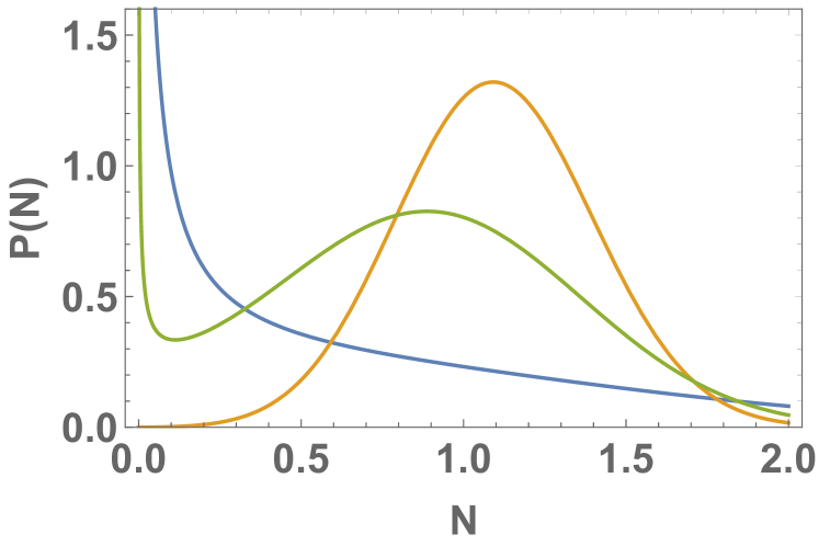
Figure 1: Common marginal distributions $\mathbf{P(N)}$, or species abundance distributions (SADs) found in real ecosystems and theoretical models. When the rate of immigration into the community is high compared to demographic noise strength, the SAD resembles a log-normal distribution (orange). However, if demographic noise dominates over migration, then there are two scenarios. A community dominated by noise has very few species surviving at high abundances and thus has an SAD that behaves like the Fisher log-series (blue). If selection is the primary driver of ecological dynamics, then a local maximum manifests at intermediate abundances (green).

II The Model

Consider a well-mixed community with a pool of $S$ different species, each with an abundance $\tilde{N}_{i}\geq 0$ where $i=1,2,\ldots S$. The population size of each species is shaped by processes such as birth, death, migration, and interactions with other species. An effective model that captures the population dynamics of such ecosystem is the stochastic Lotka-Volterra equation, which reads

$$\begin{split}\frac{d\tilde{N}_{i}}{d\tilde{t}}&=\tilde{\lambda}+\frac{\tilde{r}_{i}}{\tilde{K}_{i}}\tilde{N}_{i}\left(\tilde{K}_{i}-\tilde{N}_{i}-\sum_{j\neq i}\tilde{\alpha}_{ij}\tilde{N}_{j}\right)\\ &\phantom{=}+\sqrt{2\tilde{D}\tilde{N}_{i}}\eta_{i}(\tilde{t})\end{split}$$ (1)

In this community, a species can increase in abundance by immigrating from an external species pool at a rate $\tilde{\lambda}$, or by reproducing at a rate $\tilde{r}_{i}$. However, their population sizes cannot grow indefinitely due to intraspecies and interpecies competition for limited resources. In the absence of other species, the ecosystem can only sustain a finite number of individuals and this abundance ceiling is enforced by the carrying capacity $\tilde{K}_{i}$ and is manifested in a quadratic density-dependent death term. As for competition between different species, we make a simplifying assumption that resource dynamics occur much faster than population dynamics. As a result, interactions between species $i$ and $j$ are effectively modeled by a bilinear interaction term with a symmetric interaction matrix $\{\tilde{\alpha}_{ij}\}$. The final term in (1) represents the demographic fluctuations. The noise $\eta_{i}(t)$ is modeled by a Wiener process with the $\langle\eta_{i}(t)\rangle=0$ and correlation $\langle\eta_{i}(t)\eta_{j}(t^{\prime})\rangle=\delta_{ij}\delta(t-t^{\prime})$, where $\langle\ldots\rangle$ represents the long time average of a quantity. This multiplicative demographic noise is interpreted according to the Ito convention. All parameters and variables in (1), along with their definitions, are summarized in Table 1

Table 1: Definition of parameters and variables in the stochastic Lotka-Volterra model and their corresponding dimensionless versions

Parameter/Variable	Dimensionless parameter/variable	Definition [with units]
$\tilde{N}_{i}$	$N_{i}=\tilde{N}_{i}/\tilde{K}$	Population size of species $i$ [abundance]
$\tilde{t}$	$t=\tilde{t}\tilde{r}_{i}\tilde{K}/\tilde{K}_{i}$	Time in generations [time]
$\tilde{r}_{i}$	$r_{i}=\tilde{r}_{i}\tilde{K}/\tilde{K_{i}}=\text{const.}$	Intrinsic growth rate of species $i$ [1/time]
$\tilde{K}_{i}$	$K_{i}=\tilde{K_{i}}/\tilde{K}$	Intrinsic carrying capacity of species $i$ [abundance]
$\tilde{K}$	$K=1$	Average carrying capacity of each species [abundance]
$\tilde{\sigma}_{K}$	$\sigma_{K}=\tilde{\sigma}_{K}/\tilde{K}$	Standard deviation of carrying capacity [abundance]
$\tilde{\alpha}_{ij}$	$\alpha_{ij}=\tilde{\alpha}_{ij}$	Interaction strength between species $i$ and $j$
$\tilde{\mu}$	$\mu=\tilde{\mu}$	Average interaction strength over all pairs of species
$\tilde{\sigma}$	$\sigma=\tilde{\sigma}$	Standard deviation in interaction strengths
$\tilde{D}$	$D=\tilde{D}/\tilde{K}$	Noise strength [abundance]
$\tilde{\lambda}$	$\lambda=(\tilde{\lambda}/\tilde{K})(\tilde{K}_{i}/(\tilde{r}_{i}\tilde{K})$	Immigration rate [abundance/time]
$\eta_{i}$		Gaussian white noise with mean zero and variance one [1/time]

To incorporate species diversity and niche differences into the model, we construct a heterogeneous random community. The carrying capacity $\tilde{K}_{i}$ is drawn randomly from the Gaussian distribution, $P(\tilde{K}_{i})\sim\mathcal{N}(\tilde{K},\tilde{\sigma}_{K})$, with $\tilde{K}$ and $\tilde{\sigma}^{2}_{K}$ being the mean and variance in carrying capacity, respectively. Similarly, we pick the interaction strengths $\tilde{\alpha}_{ij}$ from another normal distribution $P(\tilde{\alpha}_{ij})\sim\mathcal{N}(\tilde{\mu}/S,\tilde{\sigma}/\sqrt{S})$, where $\tilde{\mu}/S$ and $\tilde{\sigma}^{2}/S$ represent the mean and variance in interaction strength. These random species parameters are fixed for a given community, and are hence quenched random variables. The $1/S$ scaling in the statistics of the interaction strengths $\tilde{\alpha}_{ij}$ are important because it ensures that the population neither grows without bound nor collapses too quickly. Hence, the ecosystem has an infinite species limit that would enable a statistical physics analysis.

Including this population noise term is vital to accurately model ecosystem dynamics as growth, death, and interactions with biotic and abiotic environments are inherently stochastic processes. As such, the dynamical equations must reflect this randomness. Independent populations controlled by a constant average birth and death rate features fluctuations that follow Poisson statistics, scaling as $\sqrt{\tilde{N}_{i}}$. In reality, the presence of density dependent death, interspecific interactions, and a fluctuating environment affect the population noise as well. A quantitative prediction of ecological dynamics should include these corrections to the multiplicative noise, however, numerical studies have suggested that the qualitative phase diagram is insensitive to the precise details of the noise term [2]. Thus, it suffices to model the population fluctuations of each species by an independent Wiener process with a standard deviation, $\sqrt{N_{i}}$, modified by an effective noise strength parameter, $D$. In this model of noise, higher levels of environmental stochasticity would translate to larger values of $D$. In addition to being a reasonable noise model of complex ecosystems with both neutral and non-neutral processes, it is one of the few analytically tractable models to solve.

III Results

Before solving the model for the macro-ecological properties, we can reparameterize the Lotka-Volterrra equation in $\eqref{eq:LV_equation}$. Not only does this simplify the equation into a more general form, but it also reduces the space of parameters we need to explore and allows us to identify the effective parameters that govern the overall dynamics.

For example, instead of following the temporal dynamics of the absolute population size, we only need to measure the population of each species with respect to the average carrying capacity, i.e. $N_{i}=\tilde{N}_{i}/\tilde{K}$. In addition to normalizing the abundances, we make a simplifying assumption that $r_{i}=\tilde{r_{i}}\tilde{K}/\tilde{K}_{i}$ is a constant for all species. This allows us to rescale time for all species by $t=\tilde{t}\tilde{r}_{i}\tilde{K}/\tilde{K}_{i}$ and . As a consequence of reparameterizing $\tilde{N}_{i}$ and $\tilde{t}$, we rescale the noise term and define a new dimensionless parameter $D=(\tilde{D}/\tilde{K})(\tilde{K}_{i}/(\tilde{r}_{i}\tilde{K}))^{2}$. Since the second term in the parentheses is a constant, then the relevant scaling parameter for the noise is $\tilde{D}/\tilde{K}$. Hence, the new dimensionless form of the stochastic LV equation is

$$\frac{dN_{i}}{dt}=\lambda+N_{i}\left(K_{i}-N_{i}-\sum_{j\neq{i}}\alpha_{ij}N_{j}\right)+\sqrt{2DN_{i}}\eta_{i}(t)$$ (2)

All conversions between eq. (1) and the dimensionless eq. (2) are summarized in the second column of Table 1.

For a given set of macro-ecological parameters, we can numerically solve (2) by first drawing the interactions and carrying capacities from their corresponding distributions, and then integrating the system of stochastic differential equations using the Milstein method [2]. This yields the population trajectory of each species over time, from which we can compute the equilibrium population statistics. Under certain parameter regimes, the simulation might not produce an SAD that is representative of the ecosystem. There can be large variations between different simulations of the same ecosystem because the population dynamics is noisy and the community can have multiple equilibrium solutions. Hence, averaging over multiple replicates of the ecosystem is required to obtain a more accurate species abundance distribution. The computational cost of running these replicated simulations makes it challenging to explore the vast parameter space and determine the boundaries that separate the ecosystem with different SAD behaviors. As such, we seek an analytical solution to eq. (2).

[figure]style=plain,subcapbesideposition=top

[]
[]
[]
[]

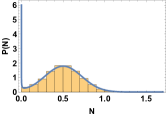
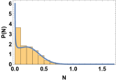
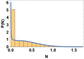
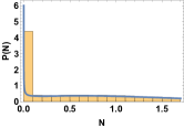
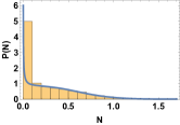
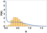
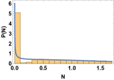
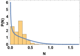
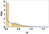
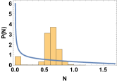
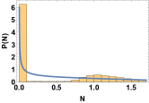
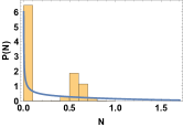
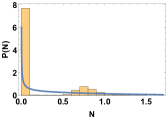
Figure 2: Marginal distributions of species abundance. Using population trajectories from integrating the stochastic Lotka-Volterra equations, we extracted the population mean of each species to construct a probability density histogram of the species abundances (orange bars). Each histogram consists of 30 ecosystem replicates each with 1000 species. Additionally, we solved for the theoretical population statistics using the iterative scheme and used these quantities to calculate the marginal distribution $P(N)$ (blue line). For our numerical computations, we set $(K,\sigma_{K})=(1,0.2)$. Each row of the figure corresponds to a different level of noise: (a) $D=0.005$, (b) $D=0.01$, (c) $D=0.1$ , and (d) $D=1.0$. Each column represents the lower left (first column), upper left (second column), lower right (third column), and upper right (fourth column) corners of the $\mu$-$\sigma$ phase diagram, respectively. First column: $(\mu,\sigma)=(1.0,0.1)$. Second column: $(\mu,\sigma)=(1.0,0.6)$. Third column: $(\mu,\sigma)=(4.0,0.1)$. Fourth column: $(\mu,\sigma)=(4.0,0.6)$. The distributions from the Milstein method and iterative scheme tend to agree for small values of $D$, but tend to be different as we increase the noise level.Furthermore, as we move toward the lower right diagrams, noise increases and the variability in interactions decreases, corresponding to the neutral-like regime. The theoretical probability distribution of species abundances (blue) start to look more generic with a rapid decay towards zero as $N$ increases and a divergence at $N=0$. This is quite reminiscent of the Fisher log-series distribution commonly found in neutral ecosystems except with a continuous $N$ rather than a discrete one.

III.1 Analytical Solution

To solve eq.(2) analytically, we transform it into the corresponding Fokker-Planck equation (FPE). In exchange for the exact population trajectory of each species, we gain access to the distribution of population sizes over time. As we are only concerned with the ecosystem at long times, we only need to solve for the stationary joint distribution of abundances of all species, $P_{S}(\{N_{i}\})$. Since the interaction matrix $\alpha_{ij}$ is symmetric, we can find an exact solution that resembles the Boltzmann distribution from statistical physics.

Even with the stationary joint distribution, extracting population statistics for a representative species from $P_{S}(\{N_{i}\})$ remains challenging due to the quenched random variables $K_{i}$ and $\alpha_{ij}$. The joint distribution for all species is also rather uninformative due to sheer number of species represented in the distribution. Instead, distributions and statistics of a representative species of the community are preferred. Long-time average population statistics such as the mean $\langle N_{i}\rangle$ and second moment $\langle N_{i}^{2}\rangle$ in abundance generally depend on the exact values of carrying capacities $K_{i}$, interactions $\alpha_{ij}$, and the abundance of all other species. However, in the limit $S\rightarrow\infty$ where the community is highly diverse, macro-ecological statistics simplify and only depend on the bulk parameters $D,K,\sigma_{K},\mu,$ and $\sigma$. To handle the quenched random variables and obtain the statistics of a representative species, we draw on techniques from the physics of disordered systems.

Naively, one could treat the interaction field term $h_{i}=\sum_{j=1}\alpha_{ij}N_{j}$ as a sum of many independent random variables, and therefore be approximated by its mean via the law of large numbers. This is the naive mean field approach and it yields the incorrect population statistics. Let us consider the population dynamics of species $i$. Changes in the abundance $N_{i}$ ripples throughout the community, generating fluctuations in the population sizes $N_{j}$ of other species and hence $h_{i}$. In turn, this change in abundances of other species in the community affects the population of species $i$. It turns out that the fluctuations in $h_{i}$ are of the same order as its mean, and therefore cannot be neglected [17, 18, 19, 20]. To truly capture these reactions and correlations in the community, we rely on the replica symmetric cavity method from the physics of disordered systems. .

The cavity method starts by introducing a new species $0$ into the community. In the thermodynamic limit $S\rightarrow\infty$, the community with $S+1$ species exhibits exhibits the same statistical properties as the original one with $S$ species. Now, let us define a new cavity field $h_{c}=\sum_{j=1}^{S}\alpha_{0j}N_{j}$, the local field felt by new species 0 due to interactions with all of the original species. By construction, these new interaction strengths $\alpha_{0j}$ are completely uncorrelated to the abundances $N_{j}$. Hence, the advantage of the replica symmetric cavity method is that we can leverage the central limit theorem and treat the cavity field $h_{c}$ as a Gaussian random variable with distribution $P(h_{c})$ instead of a quantity that depends on the original populations $\{N_{j}\}$.

Now, upon replacing the interaction term with $h_{c}$, we can integrate over $h_{c}$ to obtain a marginal distribution for the new species, $P_{S+1}(N_{0})$ (See Supplementary Information). From this marginal distribution, we can extract the population statistics of species 0. Given that the species pool is large, $S\rightarrow\infty$, then the statistics of species 0 are no different than any other species in the $S+1$ ecosystem. Although the invasion of the new species can cause the community to reshuffle and the equilibrium abundances of each species to change, the overarching statistics of the entire ecosystem and the species abundance distribution should remain unaltered. Namely, the marginal distribution for a representative species is

$$P_{S+1}(N_{0})=\int\frac{Dz}{\mathcal{N}(z)N_{0}^{1-\beta\lambda}}\exp\left[-\frac{\beta}{2}\left((1-\sigma^{2}\beta\Delta q)N_{0}^{2}-2(K-\mu\overline{\langle N\rangle}+\sqrt{\sigma_{K}^{2}+q\sigma^{2}}z)N_{0}\right)\right]$$ (3)

Here, $\overline{\langle...\rangle}$ represents the quenched average of a population statistic, where the average is taken over long times and the ensemble of possible ecological communities, i.e. the distribution of possible $\alpha_{ij}$ and $K_{i}$. So, $\overline{\langle N\rangle}$, $\overline{\langle N^{2}\rangle}$, $q=\overline{\langle N\rangle^{2}}$, and $\Delta q=\overline{\langle N^{2}\rangle}-\overline{\langle N\rangle^{2}}$ represent the quenched mean population size, the quenched mean squared abundance, the quenched average of the square of the mean abundance, and the quenched variance in population size, respectively. The equations for these quantities can be derived using the cavity method and they must be computed self-consistently. Furthermore, we define $\beta=1/D$ as the inverse ”temperature” of the community and $\mathcal{N}(z)$ as the normalization of the distribution. Also, note that the marginal distribution in (3) consists of integrating a function over a Gaussian random variable $Dz=dz~{}e^{-z^{2}/2}$, which captures the ensemble average over all possible ecosystems. The derivation of the marginal distribution is detailed in the Supplementary Information.

III.2 Comparing Numerical to Analytical Marginal Distributions

To verify our marginal distribution in equation (3), we compare it to the results of numerical analysis of the stochastic Lotka-Volterra equation. As shown in Fig. 2, the population trajectories of 1000 species are computed in 30 replicate ecosystems (with parameters $D,K,\sigma_{K},\mu,\sigma,\lambda$) and their long-time equilibrium abundances $\langle N\rangle$ are collected into a histogram and normalized to construct a probability density function.

First, for many parameter sets, the constructed histogram generally agrees with the corresponding marginal distributed computed from equation (3). When the strength of stochasticity $D$ is high, there tends to between the near-extinct species and the more abundant species. This is expected in numerical simulations as high levels of noise can quickly drive rare species to extinction. Only those with higher abundances would have a good chance of overcoming the noise and surviving. Despite some mismatch between numerical histograms and the theoretical marginal distribution, the quenched statistics $\overline{\langle N\rangle},\overline{\langle N^{2}\rangle},q,$ and $\Delta q$ calculated from the histogram match those computed self-consistently from the cavity method. The comparisons of the quenched statistics are shown in Fig. 3.

Second, the theoretical marginal distributions tend to fall into the typical categories of species abundance distributions. As seen in Fig. 3, an ecosystem where noise levels $D$ are low and species are less competitive (i.e. when $\mu$ is low) tend to have SADs that have one internal mode at high populations and an integrable singularity at zero abundance. On the other hand, ecosystems with high levels of stochasticity and stronger competition exhibit SADs that resemble the Fisher log-series with a monotonic decay in probability density as abundance increases. In addition to these distributions, there are SADs with an inflection point. The parameters corresponding to these communities represent the transition point that separate the ecosystems with log-series-like SADs from those with an internal mode.

There is another transition line that is characterized by the balance of stochastic effects from demographic noise and migration. From the marginal distribution in eq.(3), when there is a net migration away from the community to other ecosystems, $\beta\lambda<0$, then $P_{S+1}(N_{0})$ contains a non-integrable singularity. Hence, the steady-state of the stochastic LV equations is a delta-function at $N_{0}=0$ with all species ultimately going extinct. If $0<\beta\lambda<1$, then the SADs have an integrable singularity and a possible internal mode, as seen in Fig. 3. However, if the effects of immigration is stronger than demographic stochasticity, $\beta\lambda>1$, then the singularity disappears. All species can be supported at least by immigration and the SAD has a peak with few species at very low and very high abundances. Although this type of SAD is not the log-normal distribution, it shares many of its general characteristics and agrees qualitatively with neutral theories of local communities.

[figure]style=plain,subcapbesideposition=top

[] []
[] []

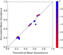
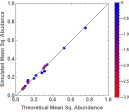
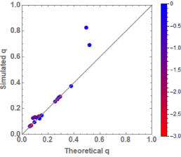
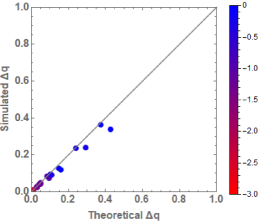
Figure 3: A comparison between population statistics computed from solving the theoretical self-consistent equations and integrating the LV equations. Each plot corresponds to a different statistics: (a) the quenched mean abundance $\overline{\langle N\rangle}$, (b) the quenched mean squared abundance $\overline{\langle N^{2}\rangle}$, (c) $q=\overline{\langle N\rangle^{2}}$, and (d) $\Delta q=\overline{\langle N^{2}\rangle-\langle N\rangle^{2}}$. The quantities obtained from either method tend to agree with each other, however there are some deviations especially for cases where the noise level $D$ becomes large.

III.3 SAD Phase Diagram

With the gamut of possible SADs characterized within this stochastic LV model, we now explore the range of macro-ecological parameters that give rise to each class of SADs and the boundaries separating the different regimes. In Fig. 4, we logarithmically sweep through the noise strength $D$ and produce 50 $\times$ 50 phase diagrams in $\mu-\sigma$ space that depicts the location of the secondary maximum, if it exists. Macro-ecological parameters such as the carrying capacity statistics $(K,\sigma_{K})$ are fixed at $(1.0,0.2)$, and the migration rate is set such that $\beta\lambda=0.5$.

At high levels of stochasticity, predominantly cooperative communities ($\mu<0$) are able to maintain coexistence of many species at high abundances whereas competition results in many species going extinct. Although some mutualism can protect coexistence, it is not without caveats. If mean cooperation is too strong ($\mu<-1$) or if the heterogeneity of interaction strengths $\sigma$ is too high, the quenched statistics of the community, $\overline{\langle N\rangle}$ and $\Delta q=\overline{\langle N^{2}\rangle-\langle N\rangle^{2}}$, both diverge. In this region, the ecosystem is unstable and the positive feedback between different species causes all populations to grow unbounded [21, 22, 23, 24, 25, 26].

However, with decreasing noise strength $D$, a wider range of ecosystems are able to support a local maximum in the SAD. Low levels of mutualism continue to promote the coexistence of many species at very high abundances. As $\mu$ increases towards positive values, the ecosystem becomes more competitive and the local maximum in the species abundance distribution shifts left toward lower abundance. Although competition can give rise to stable coexistence, it is a negative feedback process and a few strong competitors can drive more species toward increasing rarity. Eventually, with stronger competition, the behavior of the SAD shifts from one exhibiting an internal mode to one that resembles the Fisher log-series. At this point, the community consists of many rare or extinct species and very few abundant species. A similar phenomenon occurs as the spread of interaction strength $\sigma$ increases. Even if the mean competition strength $\mu$ is low, a larger spread in the distribution of interaction strengths leads to the presence of more species that can easily outcompete less-fit species. Consequently, there is a transition to a log-series-like SAD as $\sigma$ increases.

However, in the small $D$ limit of predominantly competitive communities ($\mu>0$), increasing the strength and heterogeneity of interactions eventually causes the ecosystem to experience a sharp transition from a single unique equilibrium to a multiple equilibria phase. This is a distinct phase akin to the spin-glass phase in disordered system physics in which the original replica-symmetry assumption breaks down [19, 18, 25]. However, if the variation in interaction strength $\sigma$ is too great, then the ecosystem can also destabilize with many species being driven to extinction and highly competitive species growing without bound. In this multiple equilibria regime, correlations between species become larger and ever more influential in determining the population size of each species. With the increasing importance of correlations, the community becomes extremely susceptible to small perturbations with minute fluctuations causing drastic changes to the population of each species [19, 18, 21, 22, 23, 24, 25]. Details of calculations for the transition between the replica symmetric (RS) and replica symmetry breaking (RSB) phase are found in the Supplemental Information.

With the assumptions of replica symmetry and negligible correlations breaking down, our calculations of the population statistics in this RSB regime no longer hold. Instead, we must account for the multiple equilibria and the non-Gaussianity of the cavity field distribution $P(h_{c})$ to compute the correct abundance statistics and the marginal distribution $P(N)$ [19, 18]. Despite the inconsistencies in the replica symmetric calculations, the $P(N)$ in (3) still matches the histogram of equilibrium abundances obtained from numerically integrating the Lv equations. This suggests that the RS solution is not drastically different from the RSB one. Hence, we can still use the RS cavity method to obtain a qualitative picture of the behavior of SADs in the RSB regime. In fact, upon closer examination of the theoretical $P(N)$, we find a secondary maximum reemerges in the SAD albeit with a low and broad peak. Since this secondary peak is not very prominent, it becomes difficult to practically distinguish the marginal distribution $P_{S+1}(N)$ from a log-series-like distribution where there is a high representation of species with very low abundances.

Within highly diverse ecosystems, the residing species often exhibit diverse sets of traits and occupy various niches. These inherent differences between species have long been thought to be the main mechanism shaping the structure of ecosystems, and the statistics should reflect the results from niche theory. Surprisingly, many of the species abundance distributions collected from ecological data match either the Fisher log-series or lognormal-like distribution derived from neutral theory. Although Hubbell’s neutral theory imposes an unrealistic assumptions, this agreement between data and neutral theory suggests that processes which are agnostic to species identity such as ecological drift are just as vital in influencing community dynamics.

[figure]style=plain,subcapbesideposition=top

[]
[]
[]
[]
[]
[]

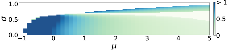
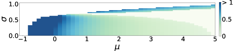
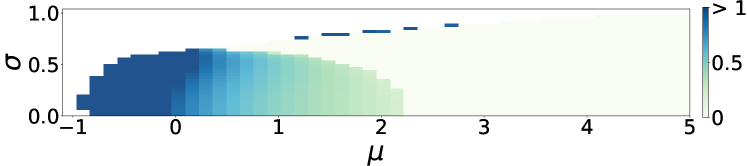
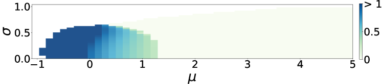
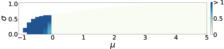
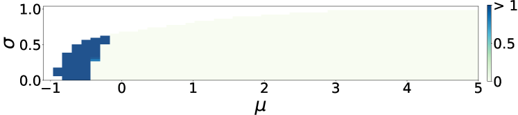
Figure 4: Phase diagram for the location of the secondary maximum of the marginal distribution. Light green corresponds to a unimodal abundance distribution that exhibits an integrable singularity at $N=0$, which is representative of the SADs of neutral communities. Blue represents ecosystems with bimodal abundance distributions with a secondary maximum at $N_{*}>0$, which is representative of SADs of communities dominated by niche differentiation. Larger values of $N_{*}$ is signified by a darker shade of blue. Each phase diagram corresponds to a different temperature: $D=$ (a) 0.005, (b) 0.01, (c) 0.05, (d) 0.1, (e) 0.5, (f) 1.0. At high levels of stochasticity ,the community is primarily dominated by neutral processes and the SADs exhibit unimodality. However, the community can still have a secondary local maximum if $-1<\mu<0$, which means that cooperation at low levels can stabilize the coexistence of many species at high abundance in the face of strong stochasticity. However, at higher levels of cooperation and larger variations $\sigma$ between species, the ecosystem destabilizes and collapses with most species going extinct and few surviving. On the other hand, as the noise level $D$ decreases, it becomes increasingly difficult for cooperative communities to maintain the secondary maximum. Instead, the secondary maximum is maintained at positive $\mu$ where the community is shaped by competition. It is also interesting to note that there is a reentrant transition as we modify the level of interaction heterogeneity in the community. In (a)-(b), the ecosystem exhibits a secondary maximum and low levels of $\sigma$ and then disappears at moderate $\sigma$. However, the secondary maximum reappears at even higher levels of $\sigma$ with a peak at a higher abundance $N_{*}$. This region seems to correspond to the RSB region where the ecosystem exhibits multiple steady states.

IV Discussion

To reconcile niche and neutral theory, we constructed a stochastic Lotka-Volterra model of a diverse community that incorporates both niche differentiation and some neutral processes common to many ecosystems. Diversity is captured through drawing each species’ carrying capacity and interspecific interactions randomly from a distribution. Although niches are not explicitly modeled, the unique set of interaction strengths for each species already partitions the community into distinct niches. As for neutral processes, we included population noise, environmental noise, and migration from a species pool.

Using techniques from the physics of disordered systems, we explored the space of macro-ecological parameters and analyzed the population statistics corresponding to each parameter set. The ”phase” diagram for the stochastic LV model is divided into several distinct regimes, with each characterized by different species abundance distributions: lognormal-like, log-series-like, or multimodal. Local communities with high rates of migration from a larger metacommunity tend to have SADs which have the semblance of a lognormal distribution with many species at intermediate abundances and few species at extremely low and high population sizes. However, once demographic stochasticity gains prominence over migration, then ecosystem’s SAD can behave in two possible ways depending on the characteristics of the interspecific interactions. For a community with uniform and weak competitive interactions, many species die out, but a subset of species survive and coexist at high abundances, resulting in a multimodal SAD. On the other hand, strong and highly heterogeneous competition generates many strong competitors that drives many species to rarity or even extinction, leaving only a few abundant species. This SAD resembles the Fisher log-series distribution. Interestingly, pushing the mean and variance in competitive strength of the community a little further destabilizes the ecosystem to have multiple equilibrium states and to be sensitive to perturbations. It turns out the SAD transitions back to one with a shallow local peak at intermediate abundances. However, if the heterogeneity in competitive interactions were increased any further, the ecosystem destabilizes again and enters an unbounded growth phase with a few surviving species growing indefinitely. For an ecosystem consisting of predominantly mutualistic interactions between species, many species survive and coexist higher abundances compared to competitive networks of species. This coexistence is remains even at higher levels of noise. However, communities that are strongly cooperative and highly heterogeneous are very unstable, collapsing to an ecosystem with few surviving species growing unbounded.

Using a stochastic Lotka-Volterra niche model, we have shown that neutral statistics need not stem from unrealistic assumptions of species equivalence. Instead they can emerge from the stochastic nature of birth-death processes, migration, and environmental fluctuations. The balance of these neutral processes with the effects of selection generated by niche partitioning and interaction heterogeneity determines whether an ecosystem displays a SAD matching niche theories or neutral theories.

Interestingly, looking at the $\mu$-$\sigma$ phase diagram at $D=1.0$ in Figure 4(a), the neutral regime with log-series-like has nearly dominated the entire phase diagram while niche phase has nearly disappeared. As the noise strength continues to rise, eventually, the only phase left is the statistically neutral one. Returning to the original un-normalized form of the stochastic LV model in equation 1, a noise strength of $\tilde{D}=D/\sqrt{K}\approx 1.0$ corresponds to a model where each species experiences wild population fluctuations of order $\sqrt{KN_{i}}$. Since the carrying capacity $K$ is quantity generally controlled by the availability of resources and other abiotic factors, then an ecosystem with strong environmental noise would generically yield population statistics and biodiversity patterns that match a neutral model. However, there is an alternative interpretation to the $\sqrt{KN_{i}}$ fluctuations. Since the abundance of the surviving dominant species $N_{i}$ tend to be proportional to their carrying capacities $K$, then generic neutral-like statistics is expected to arise when the population dynamics start to have fluctuations of order $\alpha N_{i}$. This is identical to the noise term of the stochastic Verhulst model, another common logistic model in ecology. In our model where our noise is proportional to $\sqrt{N_{i}}$, we have implicitly assumed that population fluctuations are predominantly governed by the stochasticity of the linear processes, such as birth in our case. In the stochastic Verhulst model, the $N_{i}$ scaling commonly arises from the presence of environmental fluctuations, pairwise interactions, quadratic density dependent terms, and other population regulation mechanisms [27, 28, 29, 30]. With this in mind, we would expect typical diverse ecosystems governed by birth, density dependent death, interactions, and fluctuating environments exhibit phase diagrams where the neutral phase occupies most of the parameter space. This would explain why biodiversity patterns observed across many ecosystems around the world are well-fitted by neutral theory.

In light of the implicit assumptions in modeling population noise, one fruitful direction would be to study other population noise models with scaling stronger than $\sqrt{N_{i}}$. In fact, several empirical studies have suggested that noise in some ecosystems scale with the abundance as $N_{i}^{\nu}$ where $1/2<\nu<1$. This lies between the pure demographic case and the stochastic Verhulst model [30, 6, 31, 32]. Analyzing the $\nu=1$ case and extracting the corresponding SAD ”phase” diagram would provide further insight into the prevalence of neutral statistics across ecosystems shaped in part by niche processes.

Another direction would be to relax the assumptions on the interaction network. Real ecosystems may exhibit particular network structures such as trophic layers present in the food webs [33, 33, 34]. These graphical models require us to establish a degree distribution to describe the number of interactions connected to each node (species), along with a distribution for the interaction strength. Conveniently, the cavity method from disordered systems physics provides an algorithm to solve for the dynamics on networks that are locally tree-like [20, 35, 36]. Even if the network has interaction loops, the cavity method still provides a good approximation. It would be interesting to explore how network structure, finite connectivity, and distribution of interaction strengths influence the population statistics and the ”phase” diagram of species abundance distributions.

V Acknowledgments

We would like to thank R. Marsland and W. Cui for the valuable and helpful discussions. JW was supported by the National Science Foundation Graduate Research Fellowship Program Grant No. DGE-2039656. DS was supported in part by the US National Science Foundation, through the Center for the Physics of Biological Function (PHY–1734030), by the National Institutes of Health BRAIN initiative (R01EB026943–01); and as a Simons Investigator in MMLS. PM was supported in part as a Simons Investigator in MMLS and NIH NIGMS R35GM119461 grant.

References

- Azaele et al. [2016] S. Azaele, S. Suweis, J. Grilli, I. Volkov, J. R. Banavar, and A. Maritan, Reviews of Modern Physics 88, 10.1103/RevModPhys.88.035003 (2016).
- Fisher and Mehta [2014] C. K. Fisher and P. Mehta, Proceedings of the National Academy of Sciences 111, 13111 (2014).
- Haegeman and Loreau [2011] B. Haegeman and M. Loreau, Journal of Theoretical Biology 269, 150 (2011).
- Gravel et al. [2006] D. Gravel, C. D. Canham, M. Beaudet, and C. Messier, Ecology Letters 9, 399 (2006).
- Chave [2004] J. Chave, Ecology Letters 7, 241 (2004).
- Kalyuzhny et al. [2014a] M. Kalyuzhny, E. Seri, R. Chocron, C. H. Flather, R. Kadmon, and N. M. Shnerb, The American Naturalist 184, 439 (2014a).
- Matthews and Whittaker [2014] T. J. Matthews and R. J. Whittaker, Ecology and Evolution , n/a (2014).
- Grilli [2019] J. Grilli, Laws of diversity and variation in microbial communities, preprint (Ecology, 2019).
- Hubbell [2001] S. P. Hubbell, The unified neutral theory of biodiversity and biogeography, Monographs in population biology No. 32 (Princeton University Press, Princeton, 2001).
- Chisholm and Pacala [2010] R. A. Chisholm and S. W. Pacala, Proceedings of the National Academy of Sciences 107, 15821 (2010).
- Noble et al. [2011] A. E. Noble, A. Hastings, and W. F. Fagan, Physical Review Letters 107, 10.1103/PhysRevLett.107.228101 (2011).
- Scheffer and van Nes [2006] M. Scheffer and E. H. van Nes, Proceedings of the National Academy of Sciences 103, 6230 (2006).
- Scheffer et al. [2018] M. Scheffer, E. H. van Nes, and R. Vergnon, Proceedings of the National Academy of Sciences 115, 639 (2018).
- Barabás et al. [2013] G. Barabás, R. D’Andrea, R. Rael, G. Meszéna, and A. Ostling, Oikos 122, 1565 (2013).
- Vergnon et al. [2012] R. Vergnon, E. H. van Nes, and M. Scheffer, Nature Communications 3, 10.1038/ncomms1663 (2012).
- Vergnon et al. [2013] R. Vergnon, E. H. van Nes, and M. Scheffer, Oikos 122, 1573 (2013).
- Advani et al. [2018] M. Advani, G. Bunin, and P. Mehta, Journal of Statistical Mechanics: Theory and Experiment 2018, 033406 (2018).
- Nishimori [2001] H. Nishimori, Statistical physics of spin glasses and information processing: an introduction, International series of monographs on physics No. 111 (Oxford University Press, Oxford ; New York, 2001) oCLC: ocm47063323.
- Mezard et al. [1987] M. Mezard, G. Parisi, and M. A. Virasoro, Spin glass theory and beyond, World Scientific lecture notes in physics No. v. 9 (World Scientific, Singapore ; New Jersey, 1987) oCLC: ocm14929802.
- Del Ferraro et al. [2014] G. Del Ferraro, C. Wang, D. Martí, and M. Mézard, arXiv:1409.3048 [cond-mat] (2014), arXiv: 1409.3048.
- Barbier and Arnoldi [2017] M. Barbier and J.-F. Arnoldi, bioRxiv 10.1101/147728 (2017).
- Barbier et al. [2018] M. Barbier, J.-F. Arnoldi, G. Bunin, and M. Loreau, Proceedings of the National Academy of Sciences 115, 2156 (2018).
- Bunin [2017] G. Bunin, Physical Review E 95, 10.1103/PhysRevE.95.042414 (2017).
- Bunin [2016] G. Bunin, arXiv:1607.04734 [cond-mat, physics:physics, q-bio] (2016), arXiv: 1607.04734.
- Biroli et al. [2018] G. Biroli, G. Bunin, and C. Cammarota, New Journal of Physics 20, 083051 (2018).
- Roy et al. [2019] F. Roy, G. Biroli, G. Bunin, and C. Cammarota, Journal of Physics A: Mathematical and Theoretical 52, 484001 (2019).
- Levins [1969] R. Levins, Proceedings of the National Academy of Sciences 62, 1061 (1969).
- Tuckwell and Koziol [1987] H. C. Tuckwell and J. A. Koziol, Bulletin of Mathematical Biology 49, 495 (1987).
- Hallam and Levin [1986] T. G. Hallam and S. A. Levin, Mathematical Ecology: an Introduction (Springer Berlin Heidelberg, Berlin, Heidelberg, 1986) oCLC: 840294479.
- Kessler and Shnerb [2015] D. A. Kessler and N. M. Shnerb, Physical Review E 91, 10.1103/PhysRevE.91.042705 (2015).
- Kalyuzhny et al. [2014b] M. Kalyuzhny, Y. Schreiber, R. Chocron, C. H. Flather, R. Kadmon, D. A. Kessler, and N. M. Shnerb, Ecology 95, 1701 (2014b).
- Chisholm et al. [2014] R. A. Chisholm, R. Condit, K. A. Rahman, P. J. Baker, S. Bunyavejchewin, Y.-Y. Chen, G. Chuyong, H. S. Dattaraja, S. Davies, C. E. N. Ewango, C. V. S. Gunatilleke, I. A. U. Nimal Gunatilleke, S. Hubbell, D. Kenfack, S. Kiratiprayoon, Y. Lin, J.-R. Makana, N. Pongpattananurak, S. Pulla, R. Punchi-Manage, R. Sukumar, S.-H. Su, I.-F. Sun, H. S. Suresh, S. Tan, D. Thomas, and S. Yap, Ecology Letters 17, 855 (2014).
- Allesina and Tang [2015] S. Allesina and S. Tang, Population Ecology 57, 63 (2015).
- Albert and Barabási [2002] R. Albert and A.-L. Barabási, Reviews of Modern Physics 74, 47 (2002).
- Rivoire [2005] O. Rivoire, Journal of Statistical Mechanics: Theory and Experiment 2005, P07004 (2005).
- Lokhov et al. [2015] A. Y. Lokhov, M. Mézard, and L. Zdeborová, Physical Review E 91, 10.1103/PhysRevE.91.012811 (2015).